85/08/VT Bayesian survey-based assessment of North Sea plaice (Pleuronectes platessa): extracting integrated signals from multiple surveys Johannes A. Bogaards, Sarah B. M. Kraak, and Adriaan D. Rijnsdorp

Bogaards, J. A., Kraak, S. B. M., and Rijnsdorp, A. D. 2009. Bayesian survey-based assessment of North Sea plaice (Pleuronectes platessa): extracting integrated signals from multiple surveys. – ICES Journal of Marine Science, 66: 000–000.

Dependence on a relatively small sample size is generally viewed as a big disadvantage for survey-based assessments. We propose an integrated catch-at-age model for research vessel data derived from multiple surveys, and illustrate its utility in estimating trends in North Sea plaice abundance and fishing mortality. Parameter estimates were obtained by Bayesian analysis, which allows for estimation of uncertainty in model parameters attributable to measurement error. Model results indicated constant fishing selectivity over the distribution area of the North Sea plaice stock, with decreased selectivity at older age. Whereas separate analyses of survey datasets suggested different biomass trends in the southeast than in the western and central North Sea, a combined analysis demonstrated that the observations in both subareas were compatible and that SSB has been increasing over the period 1996–2005. The annual proportion of fish that dispersed in a northwesterly direction was estimated to increase from about 10% at age 2 to 33% at age 5 and older. We also found higher fishing mortality rates than reported in ICES assessments, which could be the consequence of inadequate specification of catchability-at-age in this study or underestimated fishing mortality by the conventional ICES assessment, which relies on official landings figures. © 2009 International Council for the Exploration of the Sea. Published by Oxford Journals. All rights reserved. Keywords: Bayesian statistics, state-space models, population dynamics, survey-based assessment, plaice. Received 16 May 2008; accepted 5 February 2009. J. A. Bogaards, S. B. M. Kraak, and A. D. Rijnsdorp: Wageningen IMARES, Institute for Marine Resources and Ecosystem Studies, PO Box 68, 1970 AB IJmuiden, The Netherlands. A. D. Rijnsdorp: Aquaculture and Fisheries Group, Wageningen University, PO Box 338, 6700 AH Wageningen, The Netherlands. S. B. M. Kraak current address: Marine Institure, Rinville, Oranmore, Co. Galway, Ireland. Correspondence to A. D. Rijnsdorp: tel: +31 317 487191; fax: +31 317 487326; e-mail: Adriaan.Rijnsdorp@wur.nl. Introduction For a number of years, fishery management authorities have tried to limit fishing mortality through a total allowable catch (TAC) regime (Holden, 1994). In Europe, TAC advice is provided annually by the International Council for the Exploration of the Sea (ICES) and based on stock assessments (Daan, 1997). The science used to assess commercially exploited stocks is still dominated by population models developed some fifty years ago (Beddington et al., 2007). The most common assessments currently rely on catch-at-age data that are conventionally analysed by virtual population analysis (VPA)-type methods, e.g. eXtended Survivors Analysis (XSA; Shepherd, 1999). Such methods are dominated by commercial landings data, especially if fishing mortality for the stocks considered is high, and have few

(if any) underlying statistical distribution assumptions. Consequently, estimated stock trends may be misleading whenever official landings figures are not representative of true catches (e.g. because of illegal landings, discards, or bycatch in other fisheries), whenever significant changes in catchability have not been taken into account, or spatially heterogeneous trends in exploitation have not been properly considered (Kraak et al., 2008). Unless the TAC includes discards and/or there is 100% observer coverage, the proportion of the catch not included in the official landings figures is likely to increase with a restrictive TAC regime, leading to an increasingly biased perception of stock status.

Cook (1997) first presented an analytical model for stock assessments based solely on survey data that are insensitive to misreporting or changes in catchability. Cook’s model has formed the basis for SURBA, a computer package for the analysis of research vessel data (Needle, 2003). Although the method does not allow estimation of absolute population size, it does reveal population trends by fisheries-independent means, and provided that survey catchability is specified correctly, it yields an estimate of fishing mortality that should be comparable with that of VPA-type methods. A major drawback of survey-based assessment is that estimates of fishing mortality are often highly sensitive to noise in the data (Cook, 1997). One way to reduce this sensitivity is by constraining the estimable parameters, e.g. through the addition of penalty terms to the objective function. This impacts the outcome greatly, but without providing a clear interpretation (Needle, 2003). Given that parameter estimation in SURBA relies on a least squares method, its inability to provide a quantification of uncertainty for relevant parameters is a serious shortcoming.

As the precautionary approach has now become a key concept in fisheries management, uncertainties in stock assessments, be they survey-based or not, have to be taken into account. Numerous stochastic assessment methods have been proposed (see Lewy and Nielsen, 2003, plus the references therein), of which those that fall within the Bayesian framework have the advantage that prior beliefs about parameters can be incorporated into the estimation procedure (Punt and Hilborn, 1997). Although Bayesian methods have been criticized for their potential to give too much weight to vested interests (Cotter et al., 2004), they have proved insightful when applied to virtual population dynamics (Virtala et al., 1998; Calder et al., 2003) and to real catch-and-effort data (Millar and Meyer, 2000; Harwood and Stokes, 2003). Bayesian assessment methods based solely on survey data have not been developed until recently (e.g. Hammond and Trenkel, 2005; Porch et al., 2006).

The dependence on a relatively small sample size is generally viewed as the biggest disadvantage in performing survey-based assessments. Because the fishing effort of surveys constitutes just a fraction of the commercial fishing effort, research vessel data are inherently less precise (in the sense that observed numbers-at-age are more affected by sampling error) than commercial catch data. Although there are usually multiple surveys carried out on a particular stock, integration of different survey data in a single survey-based assessment has not been undertaken until recently (Trenkel, 2008). Most surveys have distinct characteristics regarding geographic area, time of year, and fishing gear used, which are all likely to affect the measurements. Still, this is no reason not to consider an integrated analysis of multiple surveys, especially because they already act in combination when “tuning” VPA-type assessments. Moreover, as research vessels tend to perform routine hauls at stratified random locations, survey data are sensitive to changes in the spatio-temporal distribution of a fish stock over time and across ages. This sensitivity may partly explain the poor agreement between stock trends estimated from multiple surveys separately, especially for the North Sea plaice (Pleuronectes platessa) stock (Cook, 1997; Needle, 2003), and it underscores the need for a combined analysis.

Here we propose an integrated catch-at-age model for research vessel data, derived from two surveys covering distinct parts of the distribution area of North Sea plaice. Parameters are estimated in a Bayesian context using hierarchical prior distributions for global abundance indices, which allows the estimation of measurement error. Measurement error is a consequence of the way in which samples are taken and processed in the survey, e.g. the timing of the survey or choice of fishing gear (Harwood and Stokes, 2003). The results

2

demonstrate that integrated analyses yield superior model fit to separate analyses, and partially solve the previously reported inconsistencies therein.

Methods Data Analysis is based on the age-disaggregated abundance indices obtained through the international beam trawl survey (BTS), as derived from the two Dutch research vessels RV “Isis” and RV “Tridens II”. The survey is coordinated by ICES and its primary aim is to obtain fisheries-independent stock indices, to be used in stock assessments for North Sea plaice and sole (Solea solea). The BTS is carried out with an 8 m beam trawl and takes place over a 5-week period in August/September each year. Indices are provided per ICES rectangle and reflect a standardized average of up to four hauls. Indices per ICES rectangle are combined into age-disaggregated global abundance indices by survey per year, calculated as the average number of plaice caught per hour trawled by ICES rectangle over a fixed survey area.

The BTS was carried out with RV “Isis” from 1985 on and with RV “Tridens II” from 1996 on. Together, the two research vessels roughly cover the distribution area of the North Sea plaice stock. However, the spatial distribution of sampling stations is such that RV “Isis” supplies information on the southeast of the North Sea and RV “Tridens II” information on the western and central North Sea (Figure 1). For the purpose of this analysis, we restricted ourselves to the period where information from both research vessels was available, i.e. to the 10-year period 1996–2005. The two research vessels provide data on nine age classes, with the last age class denoting a plus-group. Because the 1996 year class was misinterpreted to be the 1995 year class when it first recruited into the survey, there was no information on the first two age classes in 1997 (ICES, 2003)

Global abundance indices for the younger age classes derived from RV “Isis” were markedly higher than those from RV “Tridens II”, whereas the latter produced higher indices for older ages (Figure 2a and b). Inspection of the indices across cohorts makes it clear that VPA-type analyses cannot apply to the separate population matrices, unless one assumes that catchability varies strongly across ages, over the years, and between the two research vessels. In order to apply an integrated catch-at-age model to the combined population matrices, global abundance indices were corrected for differences in distribution area of sampling stations between the two research vessels. The survey area of RV “Isis” was 0.55 times the survey area of RV “Tridens II”, so the abundance indices of RV “Isis” were multiplied by this fraction. The same procedure was applied to the standard errors (s.e.s). Coefficients of variation (CVs) per division of the s.e.s by the corresponding global abundance indices, were transformed to s.e.s on a logarithmic scale prior to model fitting (Wasserman, 2004).

The relative s.e.s of abundance indices over the age range followed a U-shaped pattern (Figure 2c and d). The CVs at the younger age classes were particularly high for global abundance indices from RV “Tridens II”, whereas those for the older age classes were especially high for global abundance indices from RV “Isis”. This pattern arose mainly because the variation between individual indices was relatively low at high abundance indices, and vice versa.

Population dynamics model The basic equations of the population dynamics are given by Cook (1997). Briefly, a particular cohort with an initial number of recruits Ry in year y (assumed to be age 1) is described by , (1) )exp( 1

1 1,1, ∑ −

= −+−+ −=a

i iyiyaya ZRN where Na,y is the number of fish of age a in year y, and Za,y the average total mortality rate experienced from age a to age a + 1 and from year y to year y + 1. Furthermore, the usual

3

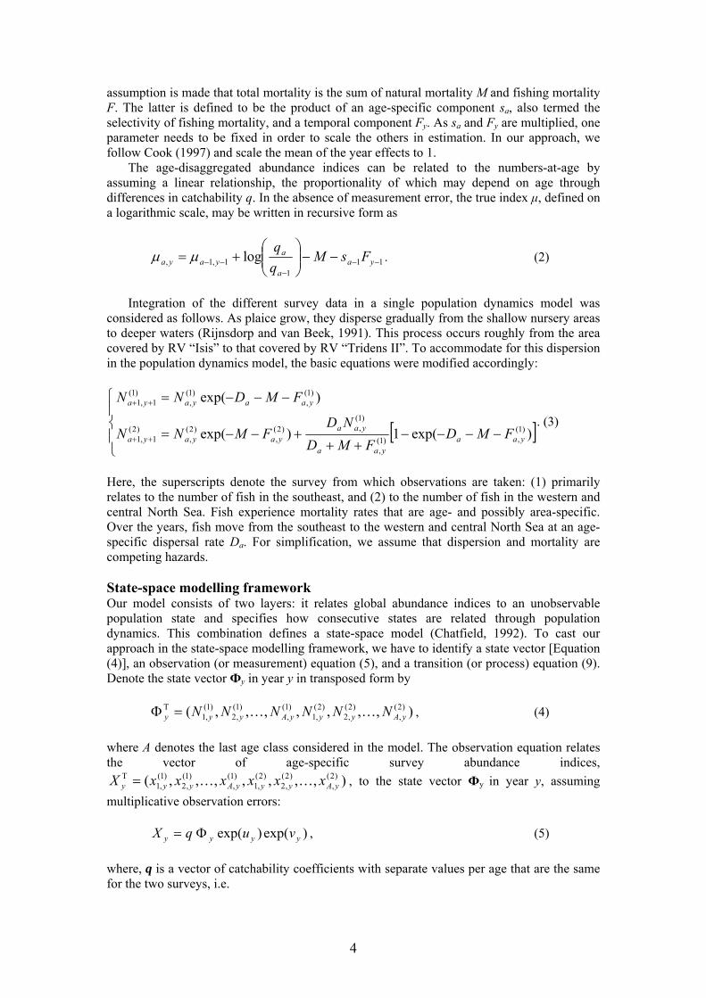
assumption is made that total mortality is the sum of natural mortality M and fishing mortality F. The latter is defined to be the product of an age-specific component sa, also termed the selectivity of fishing mortality, and a temporal component Fy. As sa and Fy are multiplied, one parameter needs to be fixed in order to scale the others in estimation. In our approach, we follow Cook (1997) and scale the mean of the year effects to 1.

The age-disaggregated abundance indices can be related to the numbers-at-age by assuming a linear relationship, the proportionality of which may depend on age through differences in catchability q. In the absence of measurement error, the true index μ, defined on a logarithmic scale, may be written in recursive form as

111

1,1, log −−−

−− −−⎟⎟⎠

⎞⎜⎜⎝

⎛+= ya

a

ayaya FsM

qq

μμ . (2)

Integration of the different survey data in a single population dynamics model was

considered as follows. As plaice grow, they disperse gradually from the shallow nursery areas to deeper waters (Rijnsdorp and van Beek, 1991). This process occurs roughly from the area covered by RV “Isis” to that covered by RV “Tridens II”. To accommodate for this dispersion in the population dynamics model, the basic equations were modified accordingly:

[ ]⎪⎩

⎪⎨

⎧

−−−−++

+−−=

−−−=

++

++

)exp(1)exp(

)exp(

)1(,)1(

,

)1(,)2(

,)2(

,)2(

1,1

)1(,

)1(,

)1(1,1

yaayaa

yaayayaya

yaayaya

FMDFMD

NDFMNN

FMDNN

. (3)

Here, the superscripts denote the survey from which observations are taken: (1) primarily relates to the number of fish in the southeast, and (2) to the number of fish in the western and central North Sea. Fish experience mortality rates that are age- and possibly area-specific. Over the years, fish move from the southeast to the western and central North Sea at an age-specific dispersal rate Da. For simplification, we assume that dispersion and mortality are competing hazards. State-space modelling framework Our model consists of two layers: it relates global abundance indices to an unobservable population state and specifies how consecutive states are related through population dynamics. This combination defines a state-space model (Chatfield, 1992). To cast our approach in the state-space modelling framework, we have to identify a state vector [Equation (4)], an observation (or measurement) equation (5), and a transition (or process) equation (9). Denote the state vector Фy in year y in transposed form by , (4) ),,,,,,,( )2(

,)2(

,2)2(

,1)1(,

)1(,2

)1(,1

TyAyyyAyyy NNNNNN KK=Φ

where A denotes the last age class considered in the model. The observation equation relates the vector of age-specific survey abundance indices,

, to the state vector Ф),,,,,,,( )2(,

)2(,2

)2(,1

)1(,

)1(,2

)1(,1

TyAyyyAyyy xxxxxxX KK= y in year y, assuming

multiplicative observation errors: , (5) )exp()exp( yyyy vuqX Φ= where, q is a vector of catchability coefficients with separate values per age that are the same for the two surveys, i.e.

4

),,,,,,,( )2()2(2

)2(1

)1()1(2

)1(1

TAA qqqqqqq KK= . (6)

The observation error is made up of two components, uy and vy. By uy we denote

measurement errors, which are assumed to be multivariate normally distributed with zero

means and covariances, and variances that depend on the survey in question (denoted by the superscript s). By v

)(2 suσ

y we denote a vector of sampling variances of the global abundance indices, which are introduced by the fact that abundance indices are estimates. The distribution of this error is also assumed to be multivariate normal with zero means and

covariances, and variances that are age- and year-specific. )(

),(2 s

yavσThe state-space model is specified by the transition equation

, (7) yyyyy wr ++Φ=Φ −1G where Gy is a (2A × 2A) updating matrix, that looks like

⎥⎥⎥⎥⎥⎥⎥⎥⎥⎥⎥⎥

⎦

⎤

⎢⎢⎢⎢⎢⎢⎢⎢⎢⎢⎢⎢

⎣

⎡

=

−−

−−−

−+−−+−−

−

−

+−+−

−−−

−

+−

++

−

+−

++

−

++−

++−

0e0000

00e00

00000000000e0

00000e000000

G

)()e1(

)()e1(

)(

)(

)2(1

)2(1

1)1(1

)1(1

)1)1(1

)1(1(

1

)2(1

)2(1

1)1(1

)1(1

)1)1(1

)1(1(

1

1)1(1

)1(1

1)1(1

)1(1

yA

AyA

ADyFAsMA

y

y

DyFsM

AyA

y

FsM

DFsMD

FsM

DFsMD

DFsM

DFsM

y

L

MMOMMMOM

LL

LL

L

MMOMMMOM

LL

LL

.

The vector ry denotes the numbers of recruits present in the month of the survey in a specific year y. It is assumed that recruits are present in both survey areas. For completeness, we introduce process error in the population dynamics through the vector wy, but only consider the case that wy has zero variance, i.e. we only consider deterministic population dynamics. Parameter estimation The traditional objective in state-space modelling is to estimate the state vector in the presence of noise (Chatfield, 1992). Our prime objective was to estimate the coefficients of the updating matrix, i.e. the parameters describing mortality and dispersion. Because the population dynamics are not defined for a plus-group, estimation was restricted to the age range 1–8. With A = 8, therefore, one needs to estimate seven coefficients for selectivity as well as nine terms describing the trend of fishing mortality over the period 1996–2005 for each survey. Numbers-at-age in the first year, Φ1, also have to be estimated, as well as the survey-specific numbers of recruits that have joined the stock since the last survey in each year. In addition, we provide an estimate of the variance attributable to measurement error for each survey. The sampling variances of the global abundance indices are calculated outside the model (as described above). Integration of the different survey data requires estimation of another seven dispersion coefficients. Consequently, the number of parameters to be estimated in the integrated model is 75 at most (for 156 data points). Separate analyses of BTS abundance indices from RV “Isis” and from RV “Tridens II” were obtained by setting all values in the age-specific migration vector D to zero. This constitutes our separate model (subsequently labelled Model A). To investigate whether the number of free parameters could be reduced without loss of predictive deviance, we performed a sequence of integrated model analyses. The general two-zone model (Model B) allows for different trends in fishing

5

mortality, different selectivity, and different measurement error between zones. Starting from this general model, we constructed nested models (Models C–I) by setting sa, Fy, or σu constant between zones or combinations thereof.

Note that natural mortality was fixed prior to parameter estimation, as were the coefficients of the catchability vector q [Equation (6)]. For comparability with ICES assessments, we set the annual rate of natural mortality to 0.1 and considered different values in sensitivity analyses (M = 0.05, 0.20, and 0.50). For comparability with Cook (1997), we assumed constant catchability across ages and survey, qa = q for both surveys. In sensitivity analyses, we also considered a slowly decreasing catchability with age, i.e. qa = 0.95qa–1, as well as a slowly increasing catchability with age, i.e. qa = (0.95)–1qa–1. Catchability coefficients were scaled to a maximum of 1 for both surveys. Parameter estimates were obtained by Bayesian analysis: )()|()|( θθθ pXpXp ∝ , (8) where p(X | θ) is the likelihood function and p(θ) the prior distribution (Gelman et al., 2004).

Previous applications of survey-based assessment (Cook, 1997; Needle, 2003) focused on the use of abundance indices in least squares estimation. In doing so, they ignored uncertainty of the estimates. One of the major advantages of Bayesian data analysis is the flexibility with which observable outcomes (indices) can be modelled conditionally on certain parameters (variance of indices), which themselves are given a probabilistic specification in terms of further parameters (Gelman et al., 2004). Such a hierarchical model enables us to separate the sampling variance of the global abundance index from measurement error. In our model, the likelihood function is the normal probability density function, defined as , (9) )|(log),|(log)|(log )(

,)(

,)(

,)(

, θμθμθ sya

sya

sya

sya pxpxp =

with ⎟⎟⎠

⎞⎜⎜⎝

⎛−−= 2)(

,)(

,

)(,

)(,)(

,)(

, )(log2

exp2

),|(log sya

sya

sya

syas

yasya xxp μ

τπ

τθμ , (10)

where, τ is the inverse of the variance (termed precision) of the index x, which is assumed to follow a lognormal distribution, and

⎟⎟⎠

⎞⎜⎜⎝

⎛−−−= 2)(

,)()(

,)(2)(2

)(, )loglog(

21exp

21)|( s

yas

asyas

us

u

sya Nqp μ

σσπθμ . (11)

This makes our model hierarchical with regard to parameter estimation, and allows the

estimation of measurement error separately from the sampling variance . We constrained the likelihood function to non-missing data.

)(2 suσ

)(2 suσ

The model parameters greatly outnumber the number of free parameters, because the joint prior for the model is determined using conditional distributions. The variance of vy is estimated outside the model, and we only consider the case that wy has zero variance, so it is

enough to specify the prior on θ = ( , , , , , ). As uninformative priors have not been identified for the current model, we aimed to construct weakly informative priors. The priors were all restricted to be positive, with uniform probability below some upper boundary (Table 1). The upper boundary for the variance of measurement error was informed by the observation that the CVs attributable to sampling variance appeared to have an upper bound of 100%, and we wanted to allow for the possibility that the variance of measurement error is larger than sampling variance. Alternatively, we fitted an inverse-gamma distribution to the sampling variance, and used this as a prior for the variance of the

)(1,s

aN )(,1syN )(s

as )(syF aD )(2 s

uσ

6

measurement error. Sensitivity of results to priors for fishing mortality, selectivity, and dispersion was examined by considering lognormal distributions that had comparable 0.95 quantiles, but lower expectation (Table 1).

Parameter estimates were obtained by Markov chain Monte Carlo (MCMC) simulation, using OpenBUGS version 1.4. In standard runs, ten chains using Gibbs sampling were run to estimate the joint posterior distribution (Gelman et al., 2004). Each run was initialized by drawing random starting points from roughly overdispersed distributions (with respect to the priors) for the free parameters. Each MCMC chain ran for 5000 iterations, after a burn-in period of 5000, and every 50th iteration was stored to remove the possible effect of autocorrelation. Thus, we stored a total of 10 times 100 realizations, from which we obtained quantiles of the posterior distributions.

Convergence was monitored in two ways. First, the trajectory of the ten chains of each parameter was inspected visually in order to assess the extent to which the chains mixed. Second, the convergence of each parameter was assessed by calculating a scale reduction factor R that roughly measures the ratio of the variance between chains to the variance within chains and should converge to 1 when stationarity is reached (Gelman et al., 2004).

Model complexity was measured by estimating the effective number of parameters pD, which can be thought of as the number of unconstrained parameters in the model (with constraints depending both on the data and on the priors). The posterior mean deviance, which is defined as –2 times the log-likelihood, has been suggested as a Bayesian measure of model fit or adequacy. This value is allowed to be negative, because a probability density can be greater than 1, e.g. if it has a small range or small standard deviation. Adding pD to the posterior mean deviance gives the deviance information criterion (DIC) for comparing models, which is approximately equivalent to Akaike’s Information Criterion in models with negligible prior information (Spiegelhalter et al., 2002). Models are penalized to have larger DIC both by the deviance (the larger this is, the worse the fit) and by pD, so favouring models with a smaller number of effective parameters. As a rule of thumb, models receiving DIC within 1–2 of the model with the lowest DIC should be considered as credible, whereas those with higher values receive considerably less support (Spiegelhalter et al., 2002).

After fitting the model, spawning-stock biomass (SSB) was calculated as the sum of the product of the estimated numbers-at-age, observed weight-at-age, and assumed maturity-at-age. Maturity was set to zero at the age of recruitment, 50% in age classes 2 and 3, and 100% at older ages. For graphical output, we used median estimates together with 95% credible intervals (ranging from the 2.5th to the 97.5th quantiles of the simulated posterior distributions). In common with conventional ICES assessments, the annual rate of fishing mortality was averaged over the age range 2–6. We compared the results of our model with the ICES assessment (ICES, 2008), to a Bayesian catch-at-age model that was made as similar as possible to the ICES assessment (Borges et al., 2007), and to a Bayesian survey-data-only model that uses the same parameterization as SURBA (Bogaards et al., 2007). Results Using the separate Model A, the estimated rate of fishing mortality was several times higher according to RV “Isis” data than to RV “Tridens II” data. There was also great disparity in the estimate of selectivity: fishing mainly affected young fish in an analysis based on RV “Isis” data, but was directed at the older age classes in the analysis with RV “Tridens II” data (Figure 3).

Models that allow for dispersion from the southeast to the western and central North Sea provided a significant improvement over separate subarea analyses, in terms of both deviance and DIC (Table 2). All integrated models demonstrated a similar departure from the separate model: fishing mortality fluctuated on a more or less similar level in the southeast as in the western and central North Sea, and was unequivocally directed at the younger age classes. The model that presumed constant selectivity between zones (Model C) seemed more adequate than the general integrated model, which allowed for differences in selectivity between zones (Model B). The models that presumed the same trend of fishing mortality in

7

the subareas had less support from the data, and those that presumed constant measurement error between zones even less. Although Model C can be regarded as a subset of Model B, its estimate of fishing mortality was markedly different (Figure 4). This was especially the case for RV “Tridens II” data, owing partly to the dependence of the fishing mortality estimate on dispersal rate.

As dispersal rate and selectivity of fishing mortality were both age-related, their estimates are not independent. High estimates of the rate of dispersal can in principle be cancelled out by adjusting the age-specific component of fishing mortality; downwards in the southeast and upwards in the western and central North Sea. Integrated models that allow for different selectivity between zones indeed showed significant correlations between dispersal rate and selectivity estimates: negative for RV “Isis” data and positive for RV “Tridens II” data (Table 3). By presuming constant selectivity between zones, the scope for trade-off between dispersal rate and selectivity was restricted: in model C, these parameter estimates were positively correlated over the age range 3–7, but the correlations were weak and meaningful at age classes 4 and 5 only. This suggests that estimates of fishing mortality in Model C were largely independent of dispersion to the western and central North Sea, whereas those in Model B might have been biased. Independent parameter estimation was impeded if it was presumed that the trend of fishing mortality in the subareas was also the same (Model F).

In the separate model (Model A), the measurement error was estimated at 0.48 (s.d. 0.08) for RV “Isis” data and at 0.47 (0.09) for RV “Tridens II” data. In the integrated models that presumed constant measurement errors between zones, the overall measurement error was consistently estimated at 0.38 (0.04). The integrated models that presumed constant measurement errors between zones yielded not only a superior model fit over that of the separate model, but also a significant reduction in the overall measurement error estimate. In the general integrated model (Model B), however, the measurement error as estimated for the RV “Isis” data increased to 0.54 (0.08), whereas that for the RV “Tridens II” data was reduced to 0.19 (0.05). Given the significant decrease in model fit by presuming constant measurement error between zones, it seems appropriate to conclude that RV “Isis” data were characterized by greater measurement error than RV “Tridens II” data.

The best-fitting model (Model C) presumed constant selectivity between zones but allowed for differences in measurement error and separate trends in fishing mortality between subareas (Figure 5). The mean annual rate of fishing mortality over the age range 2–6 fluctuated around 0.9, and was similar in the southeast and in the western and central North Sea. Closer inspection of results, however, suggests that fishing mortality in the southeast had declined up to 2001 (possibly followed by an increase to previous levels), whereas that in the western and central North Sea experienced a slight increase up to 2001 (possibly followed by a decline). The selectivity estimates clearly show that fishing mortality was directed at younger age classes. Estimates of dispersal rate increased with age, but seemed to reach a plateau around age 5. The rate of dispersion may even have decreased at older age, but estimates were imprecise. Results were not substantially influenced by the choice of priors (Figure 5).

The estimates of Model C appeared quite robust to small deviations in assumed values of natural mortality and catchability, as verified by sensitivity analyses. The estimates of dispersal rate were not affected by changes in natural mortality up to a factor of 5, whereas the estimates of fishing mortality responded as would be expected: lowering or raising M respectively resulted in slightly higher of lower estimates for fishing mortality (Figure 6). Assuming that catchability decreased with age did not influence the estimates of fishing mortality, but gave slightly lower estimates of dispersal rate above age 2. Conversely, assuming that catchability increased with age gave slightly lower estimates of dispersal rate below age 5, as well as a somewhat higher mean fishing mortality over the age range 2–6 (Figure 6).

SSB estimated using the separate Model A showed a clearly increasing trend over the period 1996–2005 for area 1 (RV "Tridens II"), and interannual variations but no trend for area 2 (RV "Isis"). In contrast, the estimates of numbers-at-age obtained by the best-fitting

8

model C indicated that SSB increased over the period 1996–2005, in both the southeast and the western/central North Sea (Figure 7).

Discussion We have here presented fisheries-independent estimates of trends in North Sea plaice abundance and fishing mortality. Our estimates are based on survey data and have been obtained by Bayesian analysis, which allows for estimation of uncertainty in the model parameters and of measurement error outside the sampling variance of the global abundance indices used. We considered integrating two surveys that cover distinct parts of the distribution area of North Sea plaice and provide a novel estimate of dispersal rate. An integrated model partially solved the disparity that arises from separate analyses of the survey datasets. Whereas separate analyses yielded different estimates of fishing mortality (over time and across ages) and divergent trends in SSB between the two subareas, integrated model analyses favoured constant selectivity of fishing mortality between zones and demonstrated compatible trends in SSB over the period 1996–2005. The different estimates of measurement error for the two survey datasets were, however, not resolved in the integrated model: RV “Isis” data were characterized by greater measurement error than RV “Tridens II” data.

The greater measurement error in the southeast could reflect reduced accuracy in the estimate of the true state of the stock for a number of reasons. A change in the spatial distribution of younger age classes has been reported, which may have affected the discarding rates of undersized plaice (van Keeken et al., 2007). Also, interference interactions between the research vessel and the commercial fleet may be involved. Interference interactions among fishing vessels may reduce the catchability of survey gear in areas with high commercial fishing effort (Gillis and Peterman, 1998; Poos and Rijnsdorp, 2007). As commercial fishing effort is much higher in the survey area of “RV Isis” than in that of “RV Tridens II” (Jennings et al., 1999), this effect may have contributed to the difference in measurement error between the two survey areas. Finally, the greater measurement error in the subarea inhabited mainly by younger age classes could also reflect a greater stochasticity in the population dynamics of immature fish, given that fluctuations in natural mortality are more likely to affect younger age classes.

Here we only considered deterministic population dynamics. Unbiased estimation of relevant parameters using a stochastic population dynamics model necessitates formulation of an appropriate error structure, and would present a major challenge and a huge improvement. The model could also be improved by explicit reference to biologically or spatially defined substocks. The current model is based on the notion that observations from different surveys are broadly related to different geographic zones, but in some ICES rectangles the two surveys do overlap. Hence, some observations from RV “Tridens II” may have been derived from the same substock as observations from RV “Isis”. Our assumption that dispersion only occurs from the area covered by RV “Isis” to the area covered by RV “Tridens II” is also a simplification. An explicit substock population dynamics model could perhaps solve these inconsistencies, because the state-space modelling framework is readily suited to facilitate the formal distinction between substocks in the population dynamics (the process equation), and to surveys with differential sampling of these underlying substocks (the measurement equation). Other potential refinements to the current approach include the specification of covariance structure in the multivariate normal likelihood for measurement error and for sampling variance. The latter could again be estimated outside the model, e.g. by close examination of errors made in otolith readings. Finally, the model could be improved by exploring parametric relationships between selectivity and age, and probably also between catchability and age. Specification of the functional form may be informed by exploratory analyses, but priors for the related parameters should be based on external information or personal belief.

Our estimates of fishing mortality were substantially higher than those reported in ICES assessments (Figure 5). Four of nine estimates of ICES fell below the 95% credible intervals of our estimates in the southeastern North Sea, and five of nine fell below those in the western

9

and central North Sea (results not shown). Assessment with a Bayesian catch-at-age model that uses the same input as the ICES assessment yields approximately similar results as the ICES assessment (Figure 8), so the higher estimates of fishing mortality are not necessarily brought about by taking a Bayesian perspective. The difference likely originates from the use of survey data only. In comparison with the ICES assessment, SURBA yielded markedly higher estimates of fishing mortality when RV “Isis” data were considered, and markedly lower estimates of fishing mortality when RV “Tridens II” data were considered (Cook, 1997; Needle, 2003). These findings have been confirmed with a Bayesian survey-data only model, using the same input and parameterization as SURBA. The question remains whether fishing mortality estimated from RV “Isis” data was overestimated, or whether that estimated solely from RV “Tridens II” data was underestimated. Our integrated model strongly suggests the latter. A single estimate for the North Sea plaice stock can be obtained by presuming a similar trend in fishing mortality as well as constant selectivity between subareas. The resulting curve clearly lies above that based on ICES estimates – 2003 being the exception (Figure 8).

North Sea plaice is managed as a single stock, so a fisheries-independent estimate of SSB would greatly facilitate stock assessment. The difficulty with using survey-based assessments to provide estimates of absolute population size is not resolved in our approach, nor can we present a single estimate of SSB. As the analytical model for research vessel data was primarily developed to examine trends in fish stocks (Cook, 1997), the finding that both subareas display compatible trends of increasing biomass when using an integrated catch-at-age model is heartening. Ways of combining multiple surveys within a formal framework to obtain a single absolute estimate of SSB are worth investigating, but the real challenge is to seek to develop an integrated management system that can respond to various biological indicators simultaneously. Our approach provides a vital addendum to the suite of indicators presently available to meet this purpose.

The integrated model incorporates an age-dependent dispersion parameter which significantly enhances model fit. Also, this model conceptually is the most credible because it reflects the underlying spatial dynamics of the stock. Our estimates suggest that, over the period 1996–2005, the annual proportion of fish that had moved in a northwesterly direction increased from about 10% at age 2 to 33% at age 5 and older. This pattern corresponds to the ontogenetic changes in distribution inferred from commercial catch rates and survey data (Rijnsdorp and van Beek, 1991). The changes in distribution with age are attributable to the gradual dispersion of maturing fish from the shallow coastal nursery grounds to deeper water offshore (Zijlstra, 1972; van Beek et al., 1989). The age at which the estimated dispersion parameter levels off corresponds to that at which females become mature (Grift et al., 2003).

Estimates of dispersal rate from abundance indices are sensitive to the timing of surveys, given the seasonal migrations of adult plaice between the spawning areas in the southern North Sea in winter and the feeding areas in the central North Sea in summer (Rijnsdorp and Pastoors, 1995; Hunter et al., 2003, 2004; Bolle et al., 2005). The estimates presented here may be somewhat conservative because they have been derived from surveys that are carried out during late summer. On the other hand, dispersion from the southeast to the western and central North Sea may have been overestimated, because we did not account for migration to the central North Sea of juvenile fish from northern nursery grounds along the Danish coast, which are not included in our surveys (Rijnsdorp and Pastoors, 1995). Clearly, there is a need for auxiliary data or an alternative parameterization if we wish to obtain unbiased information on the dispersion process.

Our analyses assumed constant M and constant q, over time and across ages, as well as between surveys. Although sensitivity analyses suggest that results are robust to small deviations from these assumptions, our estimates should still be interpreted with caution. In the absence of auxiliary information (of which there is generally none), M is commonly assumed constant, but this is not likely to reflect the actual situation. Our assumptions regarding M are the same as made in ICES assessments on the North Sea plaice stock (ICES, 2008). Nonetheless, about half of the fishing mortality rates reported by ICES fell below the 95% credible intervals of our estimates. Moreover, our estimates suggested that values of F in the southeast have increased since 2001, whereas ICES reports show a stable (or possibly

10

decreasing) F over recent years. The discrepancy in estimated trends may disappear in future analyses, given the sensitivity of mortality estimates towards the end of the observation period in catch-at-age models in general. The systematic difference in the level of F is more puzzling, especially because earlier analyses of research vessel data have also reported much higher rates of mortality than those reported in ICES assessments (Cook, 1997; Needle, 2003).

There are a several reasons why estimates of F obtained from commercial catches are lower than those that we report. First, highgrading is likely in flatfish fisheries (Rijnsdorp et al., 2007). As a result, the perception of age structure in the population becomes distorted; estimates of recruitment may be too low and survival to older age classes too high. Alternatively, our perception of survival may have been distorted by the fact that catchability-at-age is not specified adequately. Although there is some evidence of constant catchability across ages regarding plaice in the beam trawl survey (ICES, 2003), adequate specification of catchability remains elusive. Differences in catchability between the two surveys may also play a role, because there are subtle differences in gear. The RV “Tridens II” beam trawl is equipped with a flip-up rope to allow sampling on rough ground. Comparative fishing trials of both survey gears on board RV “Isis” indicated that the catchability of the flip-up beam trawl is slightly lower, of the order of 10% (Groeneveld and Rijnsdorp, 1990). Including this possible difference in catchability of the survey gears into our model would give more weight to numbers observed in the western and central North Sea than in the southeast. As these numbers are also related to the older age classes, F may have been overestimated and dispersion underestimated owing to the assumption of constant catchability between surveys. However, the impact would likely be small given the slight difference in catchability reported.

All integrated models estimate decreased selectivity of fishing mortality at older age. This is consistent with the targeting of the beam trawl fleet on sole in the southern North Sea (Quirijns et al., 2008), where younger age classes of plaice dominate. Older age classes of plaice are mainly exposed to fishing during the spawning season in the first quarter, when they aggregate on the spawning grounds in the southeastern North Sea (Rijnsdorp and Pastoors, 1995; Rijnsdorp et al., 2006). During the rest of the year, older plaice escape the heavy fishing as they disperse over the feeding grounds in the central North Sea, which is fished less intensively. Another factor that may affect the availability of fish to the fishery is the migration patterns of individual fish. Records of the seasonal migration tracks of individual plaice revealed that fish tend to repeat their seasonal migration routes (Hunter et al., 2003, 2004). Individual fish that happen to visit trawlable habitats during their seasonal migration cycle will be exposed to greater levels of fishing mortality. Hence, the proportion of fish in the population that inhabit trawlable habitats will decrease with age. The extent to which this process may affect the exploitation pattern is uncertain, but it is likely that adult plaice are less accessible to the fishery than younger age classes.

Finally, we made minimal use of the possibility of constructing informative priors. This makes our results all the more comparable with previous analyses, but neglects a main benefit of Bayesian statistics. Use of external data to formulate a functional stochastic process for the development of F over time would lead naturally to construction of informative priors. The same applies to selectivity and catchability, but there is very little information on those quantities. Moreover, as our results show, the estimates of these parameters are correlated. Even so, we demonstrate the usefulness of parameter estimation within a Bayesian framework as a flexible tool for extracting integrated signals from multiple surveys.

Acknowledgements The project was partly funded by the F-project 43911012 funded by the Ministry of LNV (Netherlands). The free use of OpenBUGS, version 1.4, and of R, version 2.3.1, is gratefully acknowledged. We thank two anonymous referees for constructive reviews. References

11

Beddington, J. R., Agnew, D. J., and Clark, C. W. 2007. Current problems in the management of marine fisheries. Science, 316: 1713–1716.

Bogaards, J. A., Borges, L., Machiels, M. A. M., Kraak, S. B. M., and Rijnsdorp, A. D. 2007. Fisheries-independent estimates of trends in North Sea plaice (Pleuronectes platessa) abundance: a Bayesian analysis of research vessel survey data. ICES Document CM 2007/O: 18. 18 pp.

Bolle, L. J., Hunter, E., Rijnsdorp, A. D., Pastoors, M. A., Metcalfe, J. D., and Reynolds, J. D. 2005. Do tagging experiments tell the truth? Using electronic tags to evaluate conventional tagging data. ICES Journal of Marine Science, 62: 236–246.

Borges, L., Kraak, S. B. M., Bogaards, J. A., and Machiels, M. A. M. 2007. 2006 stock assessment of North Sea plaice using a Bayesian catch-at-age model. Report C034/07, Wageningen IMARES, 20 pp.

Calder, C., Lavine, M., Müller, P., and Clark, J. S. 2003. Incorporating multiple sources of stochasticity into dynamic population models. Ecology, 84: 1395–1402.

Chatfield, C. 1992. The Analysis of Time Series. An Introduction, 4th edn. Chapman and Hall, London. 241 pp.

Cook, R. M. 1997. Stock trends in six North Sea stocks as revealed by an analysis of research vessel surveys. ICES Journal of Marine Science, 54: 924–933.

Cotter, A. J. R., Burt, L., Paxton, C. G. M, Fernandez, C., Buckland, S. T., and Pan, J. X. 2004. Are stock assessment methods too complicated? Fish and Fisheries, 5: 235–254.

Daan, N. 1997. TAC management in North Sea flatfish fisheries. Journal of Sea Research, 37: 321-341. Gelman, A., Carlin, J. B., Stern, H. S., and Rubin, D. B. 2004. Bayesian Data Analysis, 2nd edn.

Chapman and Hall/CRC, Boca Raton, Florida. 668 pp. Gillis, D. M., and Peterman, R. M. 1998. Implications of interference among fishing vessels and the

ideal free distribution to the interpretation of CPUE. Canadian Journal of Fisheries and Aquatic Sciences, 55: 37–46.

Grift, R. E., Rijnsdorp, A. D., Barot, S., Heino, M., and Dieckmann, U. 2003. Fisheries-induced trends in reaction norms for maturation in North Sea plaice. Marine Ecology Progress Series, 257: 247–257.

Groeneveld, K., and Rijnsdorp, A. D. 1990. The effect of the “flip-over” on the catch efficiency of the 8-m beam trawl. ICES Document CM 1990/B: 16. 13 pp.

Hammond, T. R., and Trenkel, V. M. 2005. Censored catch data in fisheries stock assessment. ICES Journal of Marine Science, 62: 1118–1130.

Harwood, J., and Stokes, K. 2003. Coping with uncertainty in ecological advice: lessons from fisheries. Trends in Ecology and Evolution, 18: 617–622.

Holden, M. J. 1994. The Common Fisheries Policy. Fishing News Books, Oxford. Hunter, E., Metcalfe, J. D., O’Brien, C. M., Arnold, G. P., and Reynolds, J. P. 2004. Vertical activity

patterns of free-swimming adult plaice in the southern North Sea. Marine Ecology Progress Series, 279: 261–273.

Hunter, E., Metcalfe, J. D., and Reynolds, J. D. 2003. Migration route and spawning area fidelity by North Sea plaice. Proceedings of the Royal Society of London, Series B, 270: 2097–2103.

ICES. 2003. Report of the Working Group on the Assessment of Demersal Stocks in the North Sea and Skagerrak, ICES Headquarters, 11–20 June 2002. ICES Document CM 2003/ACFM: 02. 759 pp.

ICES. 2008. Report of the Working Group on the Assessment of Demersal Stocks in the North Sea and Skagerrak – Spring and Autumn (WGNSSK), ICES Copenhagen. 960 pp.

Jennings, S., Alvsag, J., Cotter, A. J. R., Ehrich, S., Greenstreet, S. P. R., Jarre-Teichmann, A., Mergardt, N., et al. 1999. International fishing effort in the North Sea: an analysis of spatial and temporal trends. Fisheries Research, 40: 125–134.

Kraak, S. B. M., Daan, N., and Pastoors, M. A. 2008. The use of multiple tuning series, each covering part of a stock’s distribution area, yields biased stock assessment estimates if fishing trends vary spatially. ICES Document CM 2008/I: 12. 12 pp.

Lewy, P., and Nielsen, A. 2003. Modelling stochastic fish stock dynamics using Markov chain Monte Carlo. ICES Journal of Marine Science, 60: 743–752.

Millar, R. B., and Meyer, R. 2000. Non-linear state space modeling of fisheries biomass dynamics by using Metropolis–Hastings within-Gibbs sampling. Applied Statistics, 49: 327–342.

Needle, C. L. 2003. Survey-based assessments with SURBA. Working document to the ICES Working Group on Methods of Fish Stock Assessment, Copenhagen, February 2003.

Poos, J. J., and Rijnsdorp, A. D. 2007. An “experiment” on effort allocation of fishing vessels: the role of interference competition and area specialization. Canadian Journal of Fisheries and Aquatic Sciences, 64: 304–313.

12

Porch, C. E., Eklund, A. M., and Scott, G. P. 2006. A catch-free stock assessment model with application to goliath grouper (Epinephelus itajara) off southern Florida. Fishery Bulletin US, 104: 89–101.

Punt, A. E., and Hilborn, R. 1997. Fisheries stock assessment and decision analysis: the Bayesian approach. Reviews in Fish Biology and Fisheries, 7: 35–63.

Quirijns, F. J., Poos, J. J., and Rijnsdorp, A. D. 2008. Standardizing commercial cpue data in monitoring stock dynamics: accounting for targeting behaviour in mixed fisheries. Fisheries Research, 89: 1–8.

Rijnsdorp, A. D., Daan, N., and Dekker, W. 2006. Partial fishing mortality per fishing trip: a useful indicator for effective fishing effort in management of mixed demersal fisheries. ICES Journal of Marine Science, 63: 556–566.

Rijnsdorp, A. D., Daan, N., Dekker, W., Poos, J. J., and van Densen, W. L. T. 2007. Sustainable use of flatfish resources: addressing the credibility crisis in mixed fisheries management. Journal of Sea Research, 57: 114–125.

Rijnsdorp, A. D., and Pastoors, M. A. 1995. Modelling the spatial dynamics and fisheries of North Sea plaice (Pleuronectes platessa L.) based on tagging data. ICES Journal of Marine Science, 52: 963–980.

Rijnsdorp, A. D., and van Beek, F. A. 1991. Changes in growth of North Sea plaice (Pleuronectes platessa L.) and sole (Solea solea L.). Netherlands Journal of Sea Research, 27: 441–457.

Shepherd, J. G. 1999. Extended survivors analysis: an improved method for the analysis of catch-at-age data and abundance indices. ICES Journal of Marine Science, 56: 584–591.

Spiegelhalter, D. J., Best, N. G., Carlin, B. P., and van der Linde, A. 2002. Bayesian measures of model complexity and fit. Journal of the Royal Statistical Society, Series B (Statistical Methodology), 64: 583–639.

Trenkel, V. M. 2008. A two-stage biomass random effects model for stock assessment without catches: what can be estimated using only biomass survey indices? Canadian Journal of Fisheries and Aquatic Sciences, 65: 1024–1035.

van Beek, F. A., Rijnsdorp, A. D., and de Clerck, R. 1989. Monitoring juvenile stocks of flatfish in the Wadden Sea and the coastal areas of the southeastern North Sea. Helgoländer Wissenschaftlichen Meeresuntersuchung, 43: 461–477.

van Keeken, O. A., van Hoppe, M., Grift, R. E., and Rijnsdorp, A. D. 2007. Changes in the spatial distribution of North Sea plaice (Pleuronectes platessa) and implications for fisheries management. Journal of Sea Research, 57: 187–197.

Virtala, M., Kuikka, S., and Arjas, E. 1998. Stochastic virtual population analysis. ICES Journal of Marine Science, 55: 892–904.

Wasserman, L. 2004. All of Statistics. A Concise Course in Statistical Inference. Springer, New York, 442 pp.

Zijlstra, J. J. 1972. On the importance of the Wadden Sea as a nursery area in relation to the conservation of the southern North Sea fishery resources. Symposium of the Zoological Society of London, 29: 233–258.

Figure legends Figure 1. Spatial distribution of sampling stations of the two Dutch research vessels RV “Isis” (open circles) and RV “Tridens II” (dots) in the beam trawl survey (BTS) of August and September 2004. Figure 2. (a, b) Temporal trends, and (c, d) coefficients of variation (CVs) of the age-disaggregated abundance indices according to the two BTS research vessels. The different numbers for each year denote the age class concerned. The different points for each age indicate the CVs of the summary index in different years. Smoothed lines were obtained by a SAS Loess procedure. Figure 3. (a, b) Estimates of the average fishing mortality over ages 2–6, and (c, d) the selectivity of fishing mortality for the two BTS research vessels according to separate analyses of the survey datasets (Model A in Table 2). Thick black lines denote median estimates, and thin black lines the 95% credible intervals. Figure 4. (a, b) Estimates of the average fishing mortality over the ages 2–6, and (c, d) the selectivity of fishing mortality for the two BTS research vessels according to the three best-fitting integrated models: Model B (dashed lines), Model C (solid lines), and Model D

13

(dashed-dotted lines). Estimates from the separate Model A are given for comparison (dotted lines). See Table 2 for model specification. Figure 5. Estimates of the average fishing mortality over ages 2–6 in (a) the RV “Isis” data and (b)in the RV “Tridens II” data, and estimates of (c) dispersal rate and (d) selectivity of fishing mortality according to the best-fitting integrated model (Model C in Table 2). Thick black lines denote median estimates, and thin black lines 95% credible intervals of the simulated posterior distributions when using default priors (see Table 1). Results with alternative priors are denoted by dashed lines. Figure 6. Estimates of the average fishing mortality over ages 2–6 in (a) the RV “Isis” data and (b) in the RV “Tridens II” data, and estimates of (c) dispersal rate and (d) selectivity of fishing mortality according to the best-fitting integrated model with base-case assumptions for natural mortality and catchability (Model C in Table 2, thick solid lines) and various deviations: M = 0.05 (short-dashed lines), M = 0.20 (dashed-dotted lines), M = 0.50 (dotted lines), qa = 0.95qa–1 (thin solid lines), and qa = (0.95)–1qa–1 (long-dashed lines). Figure 7. Estimates of trends in spawning-stock biomass (SSB) from the two BTS research vessels according to (a, b) separate analyses of the survey datasets (Model A in Table 2), and (c, d) to the integrated model with constant selectivity between zones (Model C). Estimates are given as medians (thick lines) along with 95% credible intervals (thin lines) from the posterior distributions; uncertainty relates to the estimated numbers-at-age only. SSB calculated from observed numbers-at-age is denoted by circles. Figure 8. Comparison of the best-fitting integrated model (Model C in Table 2) to various other assessment models for North Sea plaice. Estimates of the average fishing mortality (top row) and selectivity of fishing mortality (bottom row) over ages 2–6 in (a, c) the RV “Isis” data, and (b, d) in the RV “Tridens II” data of the best-fitting model (thick solid lines) are compared with the ICES assessment (thin solid lines), a Bayesian catch-at-age model that uses the same input as the ICES assessment (short-dashed lines), a Bayesian survey data-only model that uses the same parameterization as SURBA (dotted lines), and an integrated model that presumes the same fishing mortality between subareas (Model F, dashed-dotted lines). Running headings J. A. Bogaards et al. Bayesian survey-based assessment of North Sea plaice

14

15

Table 1. Estimable parameters and prior distributions used in Bayesian analysis of global abundance indices of the two Dutch research vessels in the beam trawl survey (BTS). Parameter Description Default prior Alternative prior

)(,1syN Survey-specific numbers of recent

recruits in the month of the survey Uniform[0,max$] None considered

)(1,s

aN Survey-specific numbers-at-age in the first year of the data

Uniform[0,max$] None considered

)(sas Survey-specific selectivity of fishing

mortality Uniform[0,3] #LN(log 0.5, 1)

)(syF Survey-specific temporal component

of fishing mortality Uniform[0,3] #LN(log 0.5, 1)

aD Dispersal rate from RV “Isis” area to RV “Tridens II” area

Uniform[0,3] #LN(log 0.5, 1)

)(2 suσ Survey-specific variance of

measurement error Uniform[0,1] *IG(1.5, 20)

$ max is ten times maximum observed # Lognormal distribution (log mean, precision) * Inverse-gamma distribution (shape, scale) Table 2. Characteristics and model performance for nine alternative models for the North Sea plaice stock using abundance indices from two BTS research vessels covering different subareas of the North Sea. The models differ in the formulation of dispersal rate (Da), selectivity of fishing mortality (sa), trend in fishing mortality (Fy), and measurement error (σu) for the two zones s = {1,2} . Parameters were estimated with two sets of priors (see Table 1). Model Parameters Priors$ Rmax

# Deviance* pD§ DIC¶

Default 1.015 –22.9 (19.8) 136.0 113.1 A

)2(2)1(2

)2()1(

)2()1(

0

uu

yy

aa

FF

ssD

σσ ≠

≠

≠

=

Alternative 1.007 –16.1 (20.4) 133.3 117.3

Default 1.017 –40.2 (18.7) 128.9 88.7 B

)2(2)1(2

)2()1(

)2()1(

0

uu

yy

aa

FF

ssD

σσ ≠

≠

≠

>

Alternative 1.015 –34.7 (18.1) 125.8 91.1

Default 1.022 –41.4 (18.1) 128.2 86.8 C

)2(2)1(2

)2()1(

)2()1(

0

uu

yy

aa

FF

ssD

σσ ≠

≠

=

>

Alternative 1.008 –36.0 (18.5) 126.5 90.5

Default 1.025 –40.8 (18.6) 130.3 89.5 D

)2(2)1(2

)2()1(

)2()1(

0

uu

yy

aa

FF

ssD

σσ ≠

=

≠

>

Alternative 1.012 –35.7 (18.1) 129.6 93.8

16

Default 1.009 –35.4 (18.9) 131.4 96.0 E

)2(2)1(2

)2()1(

)2()1(

0

uu

yy

aa

FF

ssD

σσ =

≠

≠

>

Alternative 1.008 –29.4 (18.7) 130.6 101.2

Default 1.029 –40.3 (17.9) 131.2 90.9 F

)2(2)1(2

)2()1(

)2()1(

0

uu

yy

aa

FF

ssD

σσ ≠

=

=

>

Alternative 1.009 –35.7 (18.2) 129.9 94.2

Default 1.011 –36.4 (19.1) 132.0 95.6 G

)2(2)1(2

)2()1(

)2()1(

0

uu

yy

aa

FF

ssD

σσ =

≠

=

>

Alternative 1.007 –31.0 (18.8) 130.8 99.8

Default 1.016 –37.1 (18.4) 134.5 97.4 H

)2(2)1(2

)2()1(

)2()1(

0

uu

yy

aa

FF

ssD

σσ =

=

≠

>

Alternative 1.010 –33.0 (19.0) 132.8 99.8

Default 1.011 –35.7 (17.9) 135.1 99.4 I

)2(2)1(2

)2()1(

)2()1(

0

uu

yy

aa

FF

ssD

σσ =

=

=

>

Alternative 1.008 –33.4 (18.5) 132.7 99.3

$ Prior distributions given in Table 1 # Maximum scale reduction factor * Mean value (standard deviation) § Effective number of parameters

¶ Deviance information criterion Table 3. Correlations between estimates of the age-specific component of fishing mortality sa and dispersal rate Da in the various integrated models. For model description see Table 2. Model Vessel Age 2 Age 3 Age 4 Age 5 Age 6 Age 7 Age 8

“Isis” –0.39 –0.56 –0.56 –0.72 –0.64 –0.54 –0.45 B “Tridens II” 0.41 0.80 0.77 0.87 0.55 0.46 0.22

C –0.24 0.13 0.44 0.44 0.20 0.05 –0.10 “Isis” –0.48 –0.44 –0.62 –0.75 –0.54 –0.51 –0.41 D “Tridens II” 0.37 0.75 0.84 0.85 0.61 0.47 0.22 “Isis” –0.31 –0.60 –0.63 –0.74 –0.68 –0.64 –0.54 E “Tridens II” 0.41 0.71 0.72 0.73 0.31 0.30 0.06

F –0.31 0.23 0.47 0.54 0.26 0.10 –0.08 G –0.18 –0.09 –0.04 –0.19 –0.34 –0.27 –0.32

“Isis” –0.31 –0.56 –0.65 –0.78 –0.64 –0.65 –0.50 H “Tridens II” 0.43 0.66 0.65 0.76 0.29 0.33 0.13

I –0.27 –0.11 –0.07 –0.16 –0.26 –0.25 –0.34

Figure 1

17

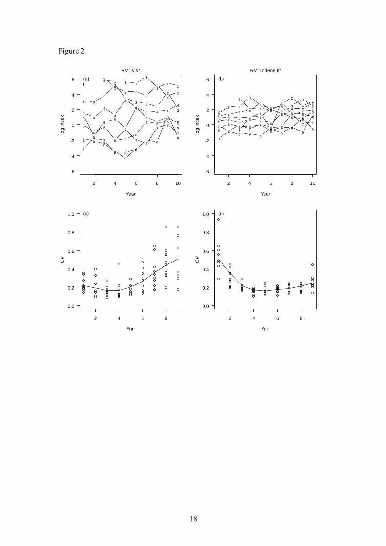
Figure 2

2 4 6 8 10

-6

-4

-2

0

2

4

6

Year

log

Inde

x

11 1 1 1

1

11 12

2

22 2

2

2

22

3 3

3

3

33 3

3

3

34

4

4

4

4

44 4 4

4

5

5

55

5

5

55

5

56

66

6 66

6 6 6 6

7

7 7 7

7

77

77

78

88

8 88

8 8

8

89 9

9

9

9

9

9

(a)

RV ''Isis''

2 4 6 8 10

-6

-4

-2

0

2

4

6

Yearlo

g In

dex

1

1

11

1

1

1 1 12

2

2 2 22

2

22

3

3 3

3

33 3 3

3

3

4 44 4

4

4 4 4 44

5 5 5 5 5

55 5 5

56 6

66 6

6

66 6

6

77

77

77 7

7

7 7

88

8 8 88

8 8

8

8

9

99 9 9

99

99

9

(b)

RV ''Tridens II''

2 4 6 8

0.0

0.2

0.4

0.6

0.8

1.0

Age

(c)

CV

2 4 6 8

0.0

0.2

0.4

0.6

0.8

1.0

Age

(d)

CV

18

Figure 3

1996 1998 2000 2002 2004

0.0

0.5

1.0

1.5

2.0

Year

mea

n

(a)

F

RV ''Isis''

1996 1998 2000 2002 2004

0.0

0.5

1.0

1.5

2.0

Yearm

ean

(b)

F

RV ''Tridens II''

1 2 3 4 5 6 7 8

0.0

0.5

1.0

1.5

2.0

Age

s

el

(c)

F

1 2 3 4 5 6 7 8

0.0

0.5

1.0

1.5

2.0

Age

s

el

(d)

F

19

Figure 4

1996 1998 2000 2002 2004

0.0

0.5

1.0

1.5

2.0

Year

mea

n

(a)

F

RV ''Isis''

1996 1998 2000 2002 2004

0.0

0.5

1.0

1.5

2.0

Yearm

ean

(b)

F

RV ''Tridens II''

1 2 3 4 5 6 7 8

0.0

0.5

1.0

1.5

2.0

Age

s

el

(c)

F

1 2 3 4 5 6 7 8

0.0

0.5

1.0

1.5

2.0

Age

s

el

(d)

F

20

Figure 5

1996 1998 2000 2002 2004

0.0

0.5

1.0

1.5

2.0

Year

mea

n

(a)

F

RV ''Isis''

1996 1998 2000 2002 2004

0.0

0.5

1.0

1.5

2.0

Yearm

ean

(b)

F

RV ''Tridens II''

1 2 3 4 5 6 7 8

0.0

0.2

0.4

0.6

0.8

1.0

Age

(c)

D

1 2 3 4 5 6 7 8

0.0

0.5

1.0

1.5

2.0

Age

s

el

(d)

F

21

Figure 6

1996 1998 2000 2002 2004

0.0

0.5

1.0

1.5

2.0

Year

mea

n

(a)

F

RV ''Isis''

1996 1998 2000 2002 2004

0.0

0.5

1.0

1.5

2.0

Yearm

ean

(b)

F

RV ''Tridens II''

1 2 3 4 5 6 7 8

0.0

0.2

0.4

0.6

0.8

1.0

Age

(c)

D

1 2 3 4 5 6 7 8

0.0

0.5

1.0

1.5

2.0

Age

s

el

(d)

F

22

Figure 7

1996 1998 2000 2002 2004

0

5

10

15

Year

SSB

(a)

RV ''Isis''

1996 1998 2000 2002 2004

0

5

10

15

YearSS

B

(b)

RV ''Tridens II''

1996 1998 2000 2002 2004

0

5

10

15

Year

SSB

(c)

1996 1998 2000 2002 2004

0

5

10

15

Year

SSB

(d)

23

Figure 8

1996 1998 2000 2002 2004

0.0

0.5

1.0

1.5

2.0

Year

mea

n

(a)

F

RV ''Isis''

1996 1998 2000 2002 2004

0.0

0.5

1.0

1.5

2.0

Yearm

ean

(b)

F

RV ''Tridens II''

1 2 3 4 5 6 7 8

0.0

0.5

1.0

1.5

2.0

Age

s

el

(c)

F

1 2 3 4 5 6 7 8

0.0

0.5

1.0

1.5

2.0

Age

s

el

(d)

F

24