bayesiannetworkclassiﬂers ... ers. anapplicationtoremotesensingimageclassiﬂcation ... been taken...

Bayesian Network Classifiers.An Application to Remote Sensing Image Classification

CRISTINA SOLARES1 and ANA MARIA SANZ2

1 Department of Applied Mathematics2 Department of Geological and Mining Engineering

University of Castilla-La Mancha

13071 Ciudad RealSPAIN

Abstract:- Different probabilistic models for classification and prediction problems are anlyzed inthis article studying their behaviour and capability in data classification. To show the capabilityof Bayesian Networks to deal with classification problems four types of Bayesian Networks areintroduced, a General Bayesian Network, the Naive Bayes, a Bayesian Network Augmented NaiveBayes and the Tree Augmented Naive Bayes. Finally, the novel application of bayesian networksin classification of spectral remote sensing images is shown.

Key-Words:- Classification, Bayesian Networks, Bayesian Network Classifiers, Naive-Bayes, RemoteSensing Image Classification, Prediction, Evidence Propagation.

1 Introduction

Classification and prediction problems occur ina wide range of situations in real life such asdisease diagnosis, image recognition, fault diag-nosis, etc.

Probabilistic models, especially those associ-ated with Bayesian Networks, are very popularas a formalism for handling uncertainty. The in-creasing number of applications developed theselast years show that this formalism has practicalvalue also (see [1], [2], [4], [7] and [8]).

Several authors have been working withBayesian Networks classifiers (see [6]). In thiswork we will do a formal study of the bayesiannetworks state-of-the-art in classification prob-lems and some experimental results are com-pared. Different models of bayesian networksare applied to the classification of remote sens-ing spectral images.

2 Bayesian Networks

A Bayesian network (BN) over X =(X1, . . . , Xn) is a pair (D,P ), where D is a di-rected acyclic graph with one node for each vari-able in X and P = {p1(x1|π1), . . ., pn(xn|πn)} isa set of n conditional probability distributions,

one for each variable, given the values of thevariables on its parent set Πi (see Castillo et al.[1]). Here xi and πi denote realizations (instan-tiations) of Xi and Πi, respectively. The jointprobability distribution (JPD) of X can thenbe written as

p(x1, x2, . . . , xn) =n

∏

i=1

pi(xi|πi). (1)

The importance of Bayesian networks reliesin that the calculation of the marginal probabil-ities of the nodes p(Xj = xj) or the conditionalprobabilities p(Xj = xj |E = e), where E is aset of evidential nodes with known values e, canbe easily calculated exploiting the JPD(1)

p(xi) =∑

xj 6∈{xi}

n∏

k=1

p(xk|x1, . . . , xk−1) (2)

p(xi|E = e) =∑

xj 6∈{xi},xj 6∈E

n∏

k=1

p(xk|x1, . . . , xk−1)

∑

xj 6∈E

n∏

k=1

p(xk|x1, . . . , xk−1)

.(3)

The problem of updating the posterior proba-bilities of a set of variables of interest whenevera new evidence becomes available is known as

Proceedings of the 6th WSEAS Int. Conf. on NEURAL NETWORKS, Lisbon, Portugal, June 16-18, 2005 (pp62-67)

evidence propagation. Castillo, Gutierrez, Hadiand Solares [2] and Castillo, Hadi and Solares[3], have been working with different algorithmsfor the exact and approximate propagation ofevidence in Bayesian networks.

2.1 Bayesian Networks as Classifiers

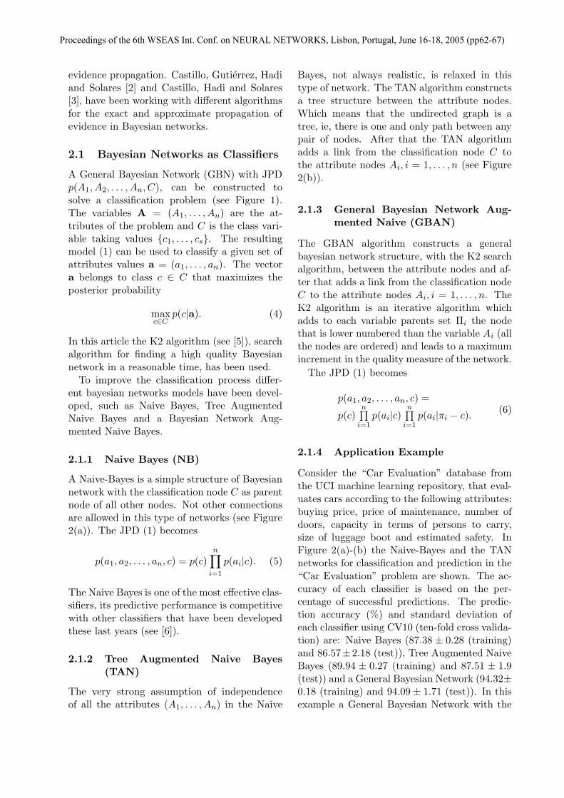
A General Bayesian Network (GBN) with JPDp(A1, A2, . . . , An, C), can be constructed tosolve a classification problem (see Figure 1).The variables A = (A1, . . . , An) are the at-tributes of the problem and C is the class vari-able taking values {c1, . . . , cs}. The resultingmodel (1) can be used to classify a given set ofattributes values a = (a1, . . . , an). The vectora belongs to class c ∈ C that maximizes theposterior probability

maxc∈C

p(c|a). (4)

In this article the K2 algorithm (see [5]), searchalgorithm for finding a high quality Bayesiannetwork in a reasonable time, has been used.

To improve the classification process differ-ent bayesian networks models have been devel-oped, such as Naive Bayes, Tree AugmentedNaive Bayes and a Bayesian Network Aug-mented Naive Bayes.

2.1.1 Naive Bayes (NB)

A Naive-Bayes is a simple structure of Bayesiannetwork with the classification node C as parentnode of all other nodes. Not other connectionsare allowed in this type of networks (see Figure2(a)). The JPD (1) becomes

p(a1, a2, . . . , an, c) = p(c)n

∏

i=1

p(ai|c). (5)

The Naive Bayes is one of the most effective clas-sifiers, its predictive performance is competitivewith other classifiers that have been developedthese last years (see [6]).

2.1.2 Tree Augmented Naive Bayes(TAN)

The very strong assumption of independenceof all the attributes (A1, . . . , An) in the Naive

Bayes, not always realistic, is relaxed in thistype of network. The TAN algorithm constructsa tree structure between the attribute nodes.Which means that the undirected graph is atree, ie, there is one and only path between anypair of nodes. After that the TAN algorithmadds a link from the classification node C tothe attribute nodes Ai, i = 1, . . . , n (see Figure2(b)).

2.1.3 General Bayesian Network Aug-mented Naive (GBAN)

The GBAN algorithm constructs a generalbayesian network structure, with the K2 searchalgorithm, between the attribute nodes and af-ter that adds a link from the classification nodeC to the attribute nodes Ai, i = 1, . . . , n. TheK2 algorithm is an iterative algorithm whichadds to each variable parents set Πi the nodethat is lower numbered than the variable Ai (allthe nodes are ordered) and leads to a maximumincrement in the quality measure of the network.

The JPD (1) becomes

p(a1, a2, . . . , an, c) =

p(c)n∏

i=1

p(ai|c)n∏

i=1

p(ai|πi − c).(6)

2.1.4 Application Example

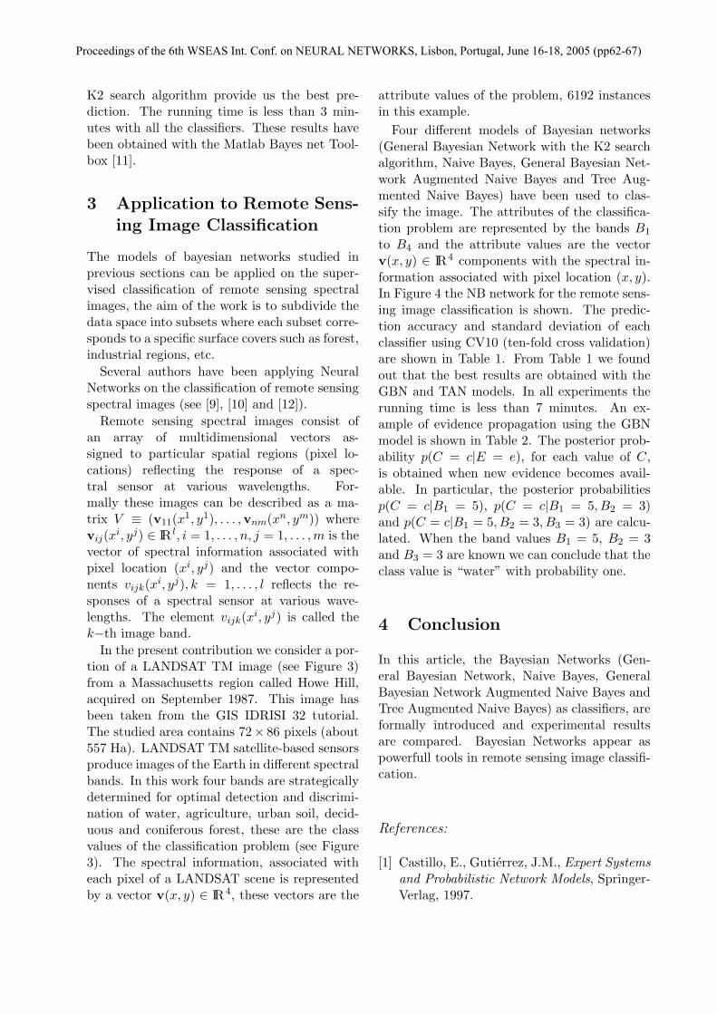
Consider the “Car Evaluation” database fromthe UCI machine learning repository, that eval-uates cars according to the following attributes:buying price, price of maintenance, number ofdoors, capacity in terms of persons to carry,size of luggage boot and estimated safety. InFigure 2(a)-(b) the Naive-Bayes and the TANnetworks for classification and prediction in the“Car Evaluation” problem are shown. The ac-curacy of each classifier is based on the per-centage of successful predictions. The predic-tion accuracy (%) and standard deviation ofeach classifier using CV10 (ten-fold cross valida-tion) are: Naive Bayes (87.38 ± 0.28 (training)and 86.57± 2.18 (test)), Tree Augmented NaiveBayes (89.94 ± 0.27 (training) and 87.51 ± 1.9(test)) and a General Bayesian Network (94.32±0.18 (training) and 94.09± 1.71 (test)). In thisexample a General Bayesian Network with the


Joint Probability Distribution

P(C,A1,A2,A3,A4,A5)=

P(C) P(A1) P(A2) P(A3)

P(A4|A1,A2) P(A5|A2,A3)

C

A3A2A1

A4A5

Evidence Propagation

P(A5=a5)

Evidence Propagation

P(A5=a5|A1=a1,A2=a2)

Classification Problem

Max P(C=c|A1=a1,A2=a2,...,A5=a5)c

Fig. 1: Example of Bayesian Network for a classification problem.

CAR

Safety Lugboot Persons Doors Maint Buying

P(CAR=unacc|safety=med,buying=med)=0.4534

max value obtained for P(CAR|safety=med,buying=med)

��e CAR acceptability is evaluated:

(a)

CAR

Safety

Lugboot

Persons

Doors

Maint

Buying

P(CAR=unacc|safety=med,buying=med)=0.5454

max value obtained for

P(CAR|safety=med,buying=med)

��e CAR acceptability is evaluated:

(b)

Fig. 2: Naive Bayes (a) and TAN (b) networks for the “Car Evaluation” problem.


K2 search algorithm provide us the best pre-diction. The running time is less than 3 min-utes with all the classifiers. These results havebeen obtained with the Matlab Bayes net Tool-box [11].

3 Application to Remote Sens-

ing Image Classification

The models of bayesian networks studied inprevious sections can be applied on the super-vised classification of remote sensing spectralimages, the aim of the work is to subdivide thedata space into subsets where each subset corre-sponds to a specific surface covers such as forest,industrial regions, etc.

Several authors have been applying NeuralNetworks on the classification of remote sensingspectral images (see [9], [10] and [12]).

Remote sensing spectral images consist ofan array of multidimensional vectors as-signed to particular spatial regions (pixel lo-cations) reflecting the response of a spec-tral sensor at various wavelengths. For-mally these images can be described as a ma-trix V ≡ (v11(x

1, y1), . . . ,vnm(xn, ym)) wherevij(x

i, yj) ∈ IR l, i = 1, . . . , n, j = 1, . . . ,m is thevector of spectral information associated withpixel location (xi, yj) and the vector compo-nents vijk(x

i, yj), k = 1, . . . , l reflects the re-sponses of a spectral sensor at various wave-lengths. The element vijk(x

i, yj) is called thek−th image band.

In the present contribution we consider a por-tion of a LANDSAT TM image (see Figure 3)from a Massachusetts region called Howe Hill,acquired on September 1987. This image hasbeen taken from the GIS IDRISI 32 tutorial.The studied area contains 72× 86 pixels (about557 Ha). LANDSAT TM satellite-based sensorsproduce images of the Earth in different spectralbands. In this work four bands are strategicallydetermined for optimal detection and discrimi-nation of water, agriculture, urban soil, decid-uous and coniferous forest, these are the classvalues of the classification problem (see Figure3). The spectral information, associated witheach pixel of a LANDSAT scene is representedby a vector v(x, y) ∈ IR4, these vectors are the

attribute values of the problem, 6192 instancesin this example.

Four different models of Bayesian networks(General Bayesian Network with the K2 searchalgorithm, Naive Bayes, General Bayesian Net-work Augmented Naive Bayes and Tree Aug-mented Naive Bayes) have been used to clas-sify the image. The attributes of the classifica-tion problem are represented by the bands B1

to B4 and the attribute values are the vectorv(x, y) ∈ IR4 components with the spectral in-formation associated with pixel location (x, y).In Figure 4 the NB network for the remote sens-ing image classification is shown. The predic-tion accuracy and standard deviation of eachclassifier using CV10 (ten-fold cross validation)are shown in Table 1. From Table 1 we foundout that the best results are obtained with theGBN and TAN models. In all experiments therunning time is less than 7 minutes. An ex-ample of evidence propagation using the GBNmodel is shown in Table 2. The posterior prob-ability p(C = c|E = e), for each value of C,is obtained when new evidence becomes avail-able. In particular, the posterior probabilitiesp(C = c|B1 = 5), p(C = c|B1 = 5, B2 = 3)and p(C = c|B1 = 5, B2 = 3, B3 = 3) are calcu-lated. When the band values B1 = 5, B2 = 3and B3 = 3 are known we can conclude that theclass value is “water” with probability one.

4 Conclusion

In this article, the Bayesian Networks (Gen-eral Bayesian Network, Naive Bayes, GeneralBayesian Network Augmented Naive Bayes andTree Augmented Naive Bayes) as classifiers, areformally introduced and experimental resultsare compared. Bayesian Networks appear aspowerfull tools in remote sensing image classifi-cation.

References:

[1] Castillo, E., Gutierrez, J.M., Expert Systems

and Probabilistic Network Models, Springer-Verlag, 1997.


1 water

2 agriculture

3 urban soil

4 deciduous forest

5 coniferous forest

CLASSIFIED IMAGE (GIS IDRISI 32)LANDSAT TM IMAGE (Spectral Band 4)

Portion of a LANDASAT TM � �� "!�#

CLASS VALUES

Fig. 3: Fourth band and classified LANDSAT TM image with IDRISI 32.

1 water

2 agriculture

3 urban soil

4 deciduous forest

5 coniferous forest

C Values

C

B3B2B1B4

v1 v2 v3 v4

v(x,y)=( v1,v2,v3,v4)

Spectral information associated with pixel (x,y)

Atribute values

Fig. 4: NB network for the remote sensing image classification.

Table 1: Prediction accuracy (%) and standard deviation with each classifier,

Classifier Training Acc. Test Acc.

NB 90.0875± 0.11 89.2927± 1.09TAN 93.9994± 0.23 93.2026± 2.57

GBAN (K2) 92.2409± 0.17 87.9035± 1.14GBN (K2) 91.3365± 0.18 90.6863± 0.39


Table 2: Marginal and posterior probabilities of class C when some band values are known (evidencepropagation), the bands are denoted as B1, B2, B3,

Class Value:c p(C = c) p(C = c|B1 = 5) p(C = c|B1 = 5, B2 = 3)

Water 0.0917 0.0917 0.9846Agriculture 0.0378 0.0010 0.0Urban Soil 0.1449 0.0078 0.0008D. Forest 0.5157 0.1204 0.0032C. Forest 0.2099 0.0987 0.0115

Class Value:c p(C = c|B1 = 5, B2 = 3, B3 = 3)

Water 1Agriculture 0.0Urban Soil 0.0D. Forest 0.0C. Forest 0.0

[2] Castillo, E., Gutierrez, J.M., Hadi, A.S., So-lares, C., Symbolic Propagation and Sensi-tivity Analysis in Gaussian Bayesian Net-works with Application to Damage Assess-ment, Journal of Artificial Intelligence in

Engineering, Vol. 11, 1997, pp.173–181.

[3] Castillo, E., Hadi, A.S., Solares, C., Learn-ing and Updating of Uncertainty in Dirich-let models, Machine Learning, Vol. 26, 1997,pp.43–63.

[4] Castillo, E., Solares, C., Gomez P., Tail Un-certainty Analysis in Complex Systems, Ar-tificial Intelligence, Vol. 96, 1997, pp.395–419.

[5] Cooper, G.F., Herskovitz, E., A BayesianMethod for the Induction ol ProbabilisticNetworks from Data , Machine Learning,Vol. 9, 1992, pp.309–347.

[6] Friedman, N., Geiger, D., Goldszmidt,M., Bayesian Network Classifiers, Machine

Learning, Vol. 29,1997, pp.131–163

[7] Gamez, J.A., Moral, S.,Salmeron, A., Ad-vances in Bayesian Networks, Springer,2004.

[8] Gutierrez, J.M., Cano, R.,Cofino, A.S.,Sordo, C.M., Redes Probabilısticas y Neu-

ronales en las Ciencias Atmosfericas, SeriesMonograficas, Ministerio de Medio Ambi-

ente, 2004.

[9] He, H., Collet, C., Combining Spectral andTextural Features for Multispectral ImageClassification with Artificial Neural Net-works, International Archives of Photogram-

metry and Remote Sensing , Vol. 32, Part7-4-3 W6, 1999

[10] Liu, J., Shao, G., Zhu, H., Liu, S., An Neu-ral Network Approach for Information Ex-traction from Remotely Sensed Data, Pro-ceedings of the International Conference on

Geoinformatics , 2004, pp.655–662

[11] Murphy, K.P. The Bayes netToolbox for Matlab, Computing

Science and Statistics, Vol. 33,http://www.cs.berkeley.edu/murphyk/Bayes/bnt.html

[12] Villmann, T., Erzsebet, M., Hammer, B.,Neural maps in remote sensing image analy-sis, Neural Networks, Vol.16, 2003, pp.389–403

Acknowledgments:The authors are indebted to the Spanish Ministry of

Science and Technology ( Project BFM2003-05695 )

for partial support.


bayesiannetworkclassiﬂers ... ers. anapplicationtoremotesensingimageclassiﬂcation ... been taken...

Documents