bba 3274 qm week 6 part 2 forecasting
TRANSCRIPT

Forecasting andForecasting andRegression Models :Regression Models :
Part 2Part 2
Forecasting andForecasting andRegression Models :Regression Models :
Part 2Part 2
BBA3274 / DBS1084 QUANTITATIVE METHODS for BUSINESSBBA3274 / DBS1084 QUANTITATIVE METHODS for BUSINESS
byStephen Ong
Visiting Fellow, Birmingham City University Business School, UK
Visiting Professor, Shenzhen University

Today’s Overview Today’s Overview

Learning ObjectivesLearning Objectives11.11. Understand and know when to use Understand and know when to use
various families of forecasting models.various families of forecasting models.
12.12. Compare moving averages, Compare moving averages, exponential smoothing, and other exponential smoothing, and other time-series models.time-series models.
13.13. Seasonally adjust data.Seasonally adjust data.
14.14. Understand Delphi and other Understand Delphi and other qualitative decision-making qualitative decision-making approaches.approaches.
15.15. Compute a variety of error measures.Compute a variety of error measures.

5-4
Forecasting Models : OutlineForecasting Models : Outline
5.15.1 IntroductionIntroduction
5.2 5.2 Types of ForecastsTypes of Forecasts
5.35.3 Scatter Diagrams and Time SeriesScatter Diagrams and Time Series
5.45.4 Measures of Forecast AccuracyMeasures of Forecast Accuracy
5.55.5 Time-Series Forecasting ModelsTime-Series Forecasting Models
5.65.6 Monitoring and Controlling ForecastsMonitoring and Controlling Forecasts

5-5
IntroductionIntroduction
Managers are always trying to reduce Managers are always trying to reduce uncertainty and make better estimates of what uncertainty and make better estimates of what will happen in the future.will happen in the future. This is the main purpose of forecasting.This is the main purpose of forecasting. Some firms use subjective methods: seat-of-the Some firms use subjective methods: seat-of-the
pants methods, intuition, experience.pants methods, intuition, experience. There are also several quantitative techniques, There are also several quantitative techniques,
including:including: Moving averagesMoving averages Exponential smoothingExponential smoothing Trend projectionsTrend projections Least squares regression analysisLeast squares regression analysis
5-6
IntroductionIntroduction
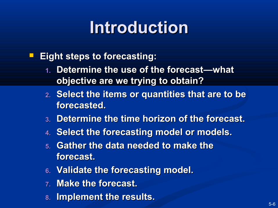
Eight steps to forecasting:Eight steps to forecasting:
1.1. Determine the use of the forecastDetermine the use of the forecast——what what objective are we trying to obtain?objective are we trying to obtain?
2.2. Select the items or quantities that are to be Select the items or quantities that are to be forecasted.forecasted.
3.3. Determine the time horizon of the forecast.Determine the time horizon of the forecast.
4.4. Select the forecasting model or models.Select the forecasting model or models.
5.5. Gather the data needed to make the Gather the data needed to make the forecast.forecast.
6.6. Validate the forecasting model.Validate the forecasting model.
7.7. Make the forecast.Make the forecast.
8.8. Implement the results.Implement the results.
IntroductionIntroduction
These steps are a systematic way of initiating, These steps are a systematic way of initiating, designing, and implementing a forecasting designing, and implementing a forecasting system.system.
When used regularly over time, data is When used regularly over time, data is collected routinely and calculations performed collected routinely and calculations performed automatically.automatically.
There is seldom one superior forecasting There is seldom one superior forecasting system.system. Different organizations may use different techniques.Different organizations may use different techniques. Whatever tool works best for a firm is the one that Whatever tool works best for a firm is the one that
should be used.should be used.

5-8
Regression Analysis
Multiple Regression
MovingAverage
Exponential Smoothing
Trend Projections
Decomposition
Delphi Methods
Jury of Executive Opinion
Sales ForceComposite
Consumer Market Survey
Time-Series Time-Series MethodsMethods
Qualitative Qualitative ModelsModels
Causal Causal MethodsMethods
Forecasting ModelsForecasting ModelsForecasting Forecasting TechniquesTechniques
Figure 5.1

5-9
Qualitative ModelsQualitative Models
Qualitative modelsQualitative models incorporate judgmental incorporate judgmental or subjective factors.or subjective factors.
These are useful when subjective factors These are useful when subjective factors are thought to be important or when are thought to be important or when accurate quantitative data is difficult to accurate quantitative data is difficult to obtain.obtain.
Common qualitative techniques are:Common qualitative techniques are: Delphi method.Delphi method. Jury of executive opinion.Jury of executive opinion. Sales force composite.Sales force composite. Consumer market surveys.Consumer market surveys.
Qualitative ModelsQualitative Models
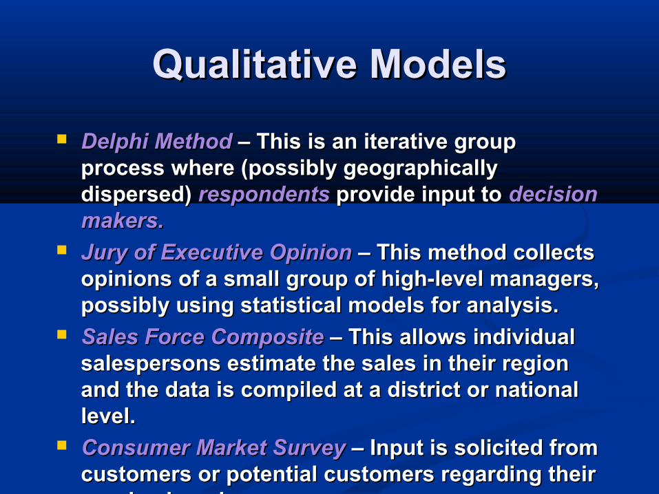
Delphi MethodDelphi Method – This is an iterative group – This is an iterative group process where (possibly geographically process where (possibly geographically dispersed) dispersed) respondentsrespondents provide input to provide input to decision decision makers.makers.
Jury of Executive OpinionJury of Executive Opinion – This method collects – This method collects opinions of a small group of high-level managers, opinions of a small group of high-level managers, possibly using statistical models for analysis.possibly using statistical models for analysis.
Sales Force Composite Sales Force Composite – This allows individual – This allows individual salespersons estimate the sales in their region salespersons estimate the sales in their region and the data is compiled at a district or national and the data is compiled at a district or national level.level.
Consumer Market SurveyConsumer Market Survey – Input is solicited from – Input is solicited from customers or potential customers regarding their customers or potential customers regarding their purchasing plans.purchasing plans.
5-11
Time-Series ModelsTime-Series Models
Time-series modelsTime-series models attempt to predict attempt to predict the future based on the past.the future based on the past.
Common time-series models are:Common time-series models are: Moving average.Moving average. Exponential smoothing.Exponential smoothing. Trend projections.Trend projections. Decomposition.Decomposition.
Regression analysis is used in trend Regression analysis is used in trend projections and one type of projections and one type of decomposition model.decomposition model.
5-12
Causal ModelsCausal Models
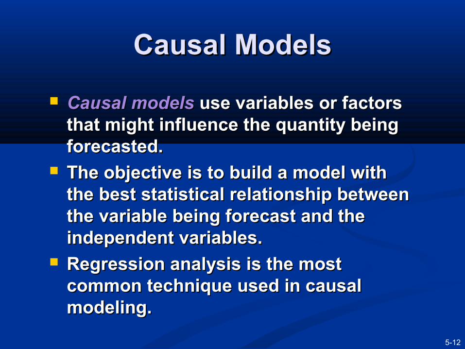
Causal modelsCausal models use variables or factors use variables or factors that might influence the quantity being that might influence the quantity being forecasted.forecasted.
The objective is to build a model with The objective is to build a model with the best statistical relationship between the best statistical relationship between the variable being forecast and the the variable being forecast and the independent variables.independent variables.
Regression analysis is the most Regression analysis is the most common technique used in causal common technique used in causal modeling.modeling.

5-13
Scatter DiagramsScatter DiagramsWacker Distributors wants to forecast sales for three different products (annual sales in the table, in units):
YEAR TELEVISION SETS RADIOS COMPACT DISC
PLAYERS
1 250 300 110
2 250 310 100
3 250 320 120
4 250 330 140
5 250 340 170
6 250 350 150
7 250 360 160
8 250 370 190
9 250 380 200
10 250 390 190
Table 5.1

5-14
Scatter Diagram for TVsScatter Diagram for TVs
Figure 5.2a
330 –
250 –
200 –
150 –
100 –
50 –
| | | | | | | | | |
0 1 2 3 4 5 6 7 8 9 10
Time (Years)
Ann
ual S
ales
of T
elev
isio
ns
(a) Sales appear to be constant
over timeSales = 250
A good estimate of sales in year 11 is 250 televisions
5-15
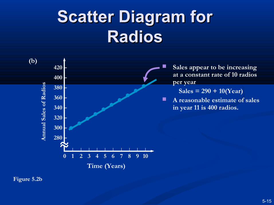
Scatter Diagram for Scatter Diagram for RadiosRadios
Sales appear to be increasing at a constant rate of 10 radios per year
Sales = 290 + 10(Year) A reasonable estimate of sales
in year 11 is 400 radios.
420 –
400 –
380 –
360 –
340 –
320 –
300 –
280 –
| | | | | | | | | |
0 1 2 3 4 5 6 7 8 9 10
Time (Years)
Ann
ual S
ales
of R
adio
s
(b)
Figure 5.2b
5-16
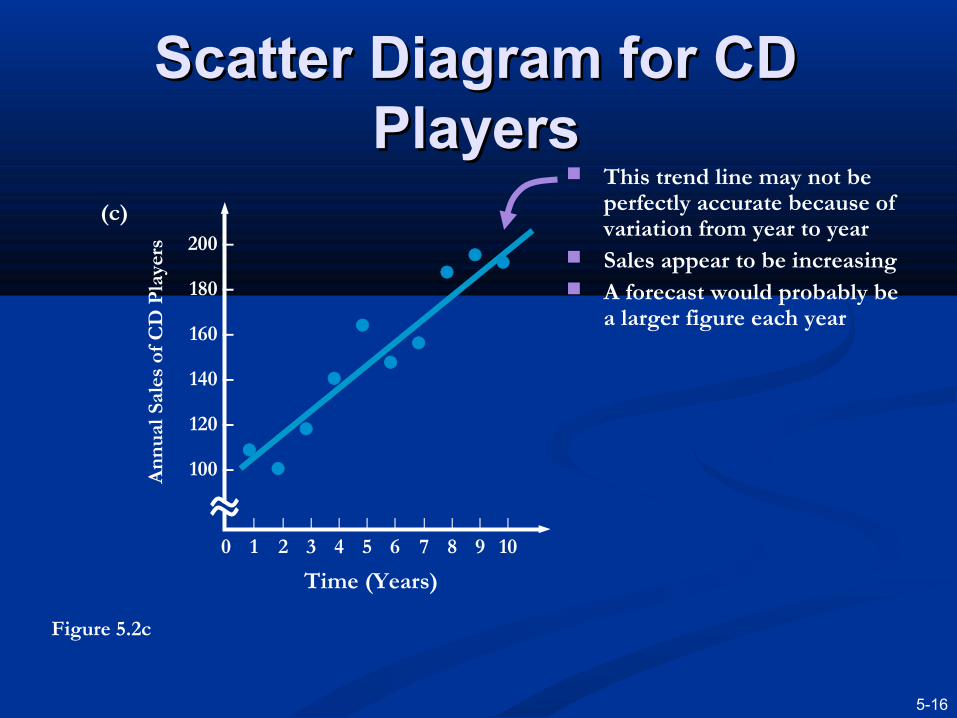
Scatter Diagram for CD Scatter Diagram for CD PlayersPlayers
This trend line may not be perfectly accurate because of variation from year to year
Sales appear to be increasing A forecast would probably be
a larger figure each year
200 –
180 –
160 –
140 –
120 –
100 –
| | | | | | | | | |
0 1 2 3 4 5 6 7 8 9 10
Time (Years)
Ann
ual S
ales
of C
D P
laye
rs
(c)
Figure 5.2c

5-17
Measures of Forecast AccuracyMeasures of Forecast Accuracy
We compare forecasted values with actual values We compare forecasted values with actual values to see how well one model works or to compare to see how well one model works or to compare models.models.
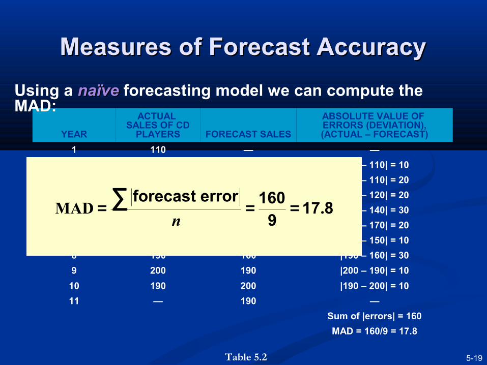
Forecast error = Actual value – Forecast value
One measure of accuracy is the mean absolutemean absolute deviationdeviation (MADMAD):
n∑=
errorforecast MAD

5-18
Measures of Forecast AccuracyMeasures of Forecast Accuracy
Using a Using a naïvenaïve forecasting model we can compute the forecasting model we can compute the MAD:MAD:
YEAR
ACTUAL SALES OF
CD PLAYERS
FORECAST SALES
ABSOLUTE VALUE OF ERRORS (DEVIATION), (ACTUAL – FORECAST)
1 110 — —
2 100 110 |100 – 110| = 10
3 120 100 |120 – 110| = 20
4 140 120 |140 – 120| = 20
5 170 140 |170 – 140| = 30
6 150 170 |150 – 170| = 20
7 160 150 |160 – 150| = 10
8 190 160 |190 – 160| = 30
9 200 190 |200 – 190| = 10
10 190 200 |190 – 200| = 10
11 — 190 —
Sum of |errors| = 160
MAD = 160/9 = 17.8
Table 5.2
5-19
Measures of Forecast AccuracyMeasures of Forecast Accuracy
YEAR
ACTUAL SALES OF CD
PLAYERS FORECAST SALES
ABSOLUTE VALUE OF ERRORS (DEVIATION), (ACTUAL – FORECAST)
1 110 — —
2 100 110 |100 – 110| = 10
3 120 100 |120 – 110| = 20
4 140 120 |140 – 120| = 20
5 170 140 |170 – 140| = 30
6 150 170 |150 – 170| = 20
7 160 150 |160 – 150| = 10
8 190 160 |190 – 160| = 30
9 200 190 |200 – 190| = 10
10 190 200 |190 – 200| = 10
11 — 190 —
Sum of |errors| = 160
MAD = 160/9 = 17.8
Table 5.2
8179
160errorforecast .MAD === ∑
n
Using a naïvenaïve forecasting model we can compute the MAD:

Measures of Forecast AccuracyMeasures of Forecast Accuracy
There are other popular measures of forecast There are other popular measures of forecast accuracy.accuracy.
The The mean squared error:mean squared error:
n∑=
2error)(MSE
The mean absolute percent error:mean absolute percent error:
%MAPE 100actualerror
n
∑=
And biasbias is the average error.

5-21
Time-Series Forecasting ModelsTime-Series Forecasting Models
A time series is a sequence of evenly A time series is a sequence of evenly spaced events.spaced events.
Time-series forecasts predict the future Time-series forecasts predict the future based solely on the past values of the based solely on the past values of the variable, and other variables are variable, and other variables are ignored.ignored.

5-22
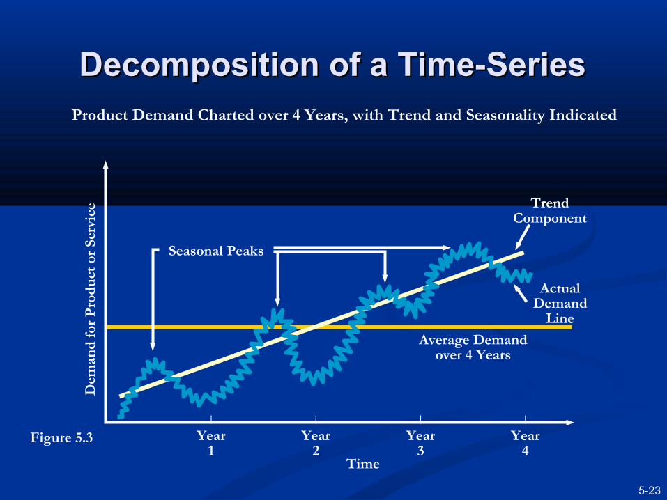
Components of a Time-SeriesComponents of a Time-Series
A time series typically has four components:A time series typically has four components:
1.1. TrendTrend ( (TT) is the gradual upward or downward ) is the gradual upward or downward movement of the data over time.movement of the data over time.
2.2. SeasonalitySeasonality ( (SS) is a pattern of demand ) is a pattern of demand fluctuations above or below the trend line that fluctuations above or below the trend line that repeats at regular intervals.repeats at regular intervals.
3.3. CyclesCycles ( (CC) are patterns in annual data that ) are patterns in annual data that occur every several years.occur every several years.
4.4. Random variationsRandom variations ( (RR) are “blips” in the data ) are “blips” in the data caused by chance or unusual situations, and caused by chance or unusual situations, and follow no discernible pattern.follow no discernible pattern.
5-23
Decomposition of a Time-SeriesDecomposition of a Time-Series
Average Demand over 4 Years
Trend Component
Actual Demand
Line
Time
Dem
and
for
Pro
duct
or
Serv
ice
| | | |
Year Year Year Year1 2 3 4
Seasonal Peaks
Figure 5.3
Product Demand Charted over 4 Years, with Trend and Seasonality Indicated

5-24
Decomposition of a Time-SeriesDecomposition of a Time-Series
There are two general forms of time-series There are two general forms of time-series models:models: The multiplicative model:The multiplicative model:
Demand = Demand = TT x x SS x x CC x x RR
The additive model:
Demand = T + S + C + R
Models may be combinations of these two forms. Forecasters often assume errors are normally distributed with a
mean of zero.

5-25
Moving AveragesMoving Averages
Moving averagesMoving averages can be used when demand is relatively steady over time.
The next forecast is the average of the most recent n data values from the time series.
This methods tends to smooth out short-term irregularities in the data series.
nn periods previous in demands of Sum
forecast average Moving =
5-26
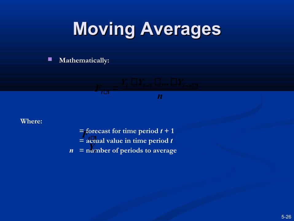
Moving AveragesMoving Averages
Mathematically:
nYYY
F ntttt
111
+−−+
+++= ...
Where:= forecast for time period t + 1= actual value in time period t
n = number of periods to averagetY1+tF
5-27
Wallace Garden SupplyWallace Garden Supply
Wallace Garden Supply wants to forecast demand for its Storage Shed.
They have collected data for the past year. They are using a three-month moving
average to forecast demand (n = 3).
5-28
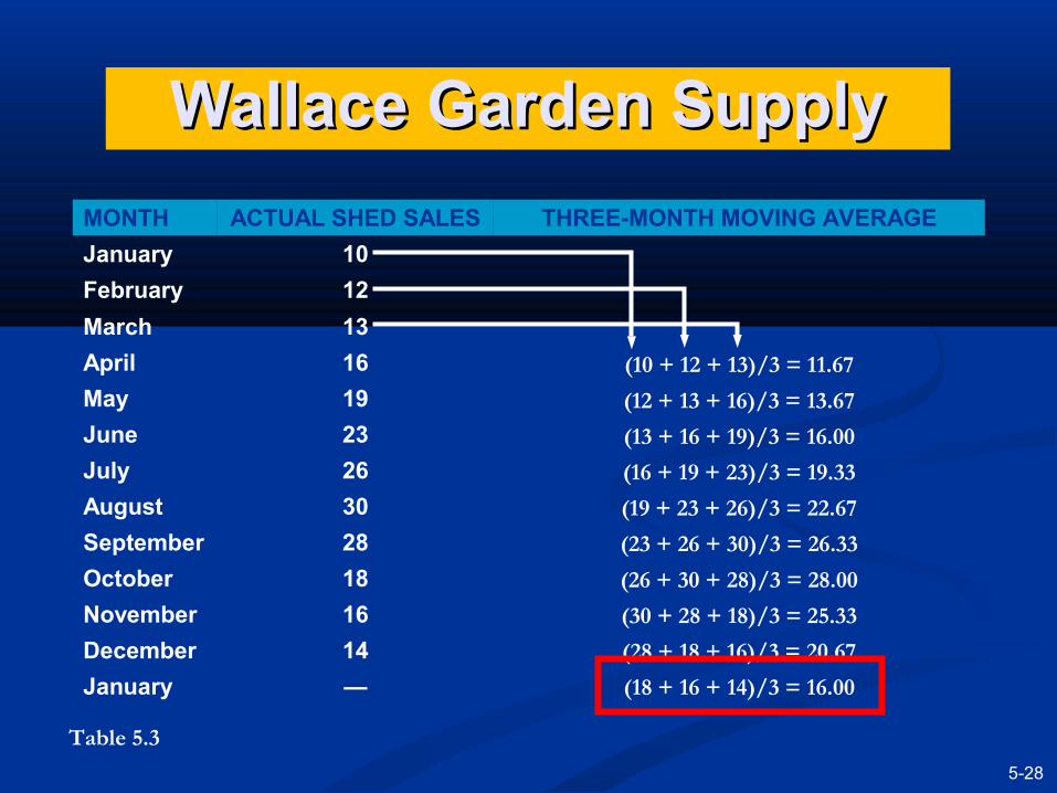
Wallace Garden SupplyWallace Garden Supply
Table 5.3
MONTH ACTUAL SHED SALES THREE-MONTH MOVING AVERAGE
January 10
February 12
March 13
April 16
May 19
June 23
July 26
August 30
September 28
October 18
November 16
December 14
January —
(12 + 13 + 16)/3 = 13.67
(13 + 16 + 19)/3 = 16.00
(16 + 19 + 23)/3 = 19.33
(19 + 23 + 26)/3 = 22.67
(23 + 26 + 30)/3 = 26.33
(26 + 30 + 28)/3 = 28.00
(30 + 28 + 18)/3 = 25.33
(28 + 18 + 16)/3 = 20.67
(18 + 16 + 14)/3 = 16.00
(10 + 12 + 13)/3 = 11.67
5-29
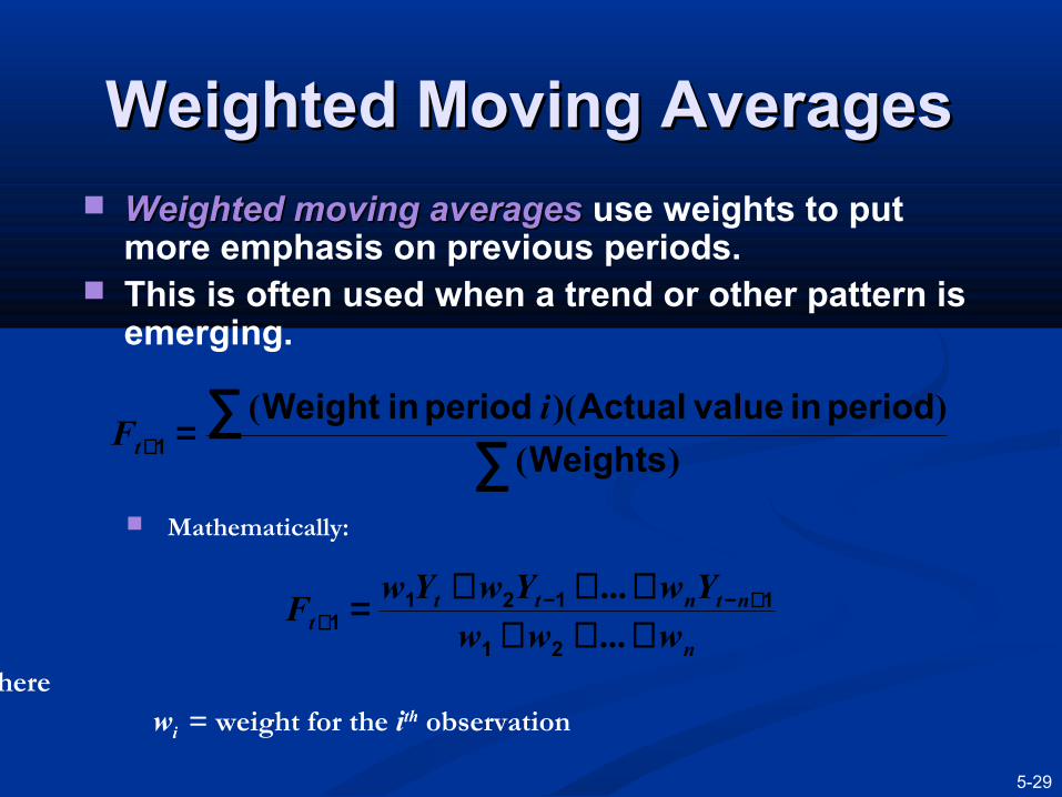
Weighted Moving AveragesWeighted Moving Averages Weighted moving averagesWeighted moving averages use weights to put
more emphasis on previous periods. This is often used when a trend or other pattern is
emerging.
∑∑=+ )(
))((
Weights
period in value Actual period inWeight 1
iFt
Mathematically:
n
ntnttt www
YwYwYwF
++++++= +−−
+ ......
21
11211
wherewi = weight for the ith observation
5-30
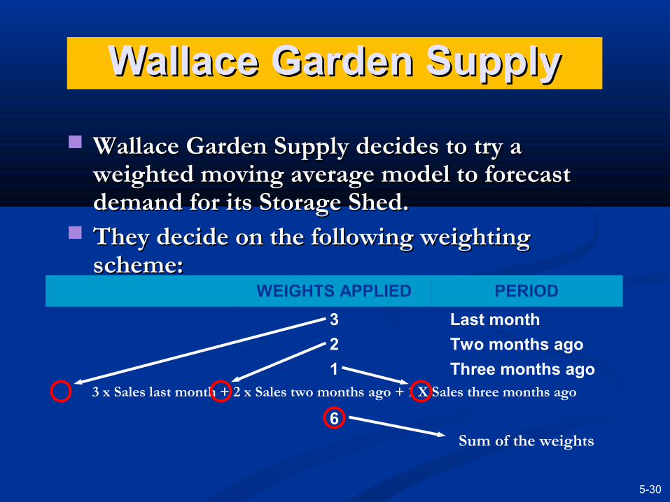
Wallace Garden SupplyWallace Garden Supply
Wallace Garden Supply decides to try a Wallace Garden Supply decides to try a weighted moving average model to forecast weighted moving average model to forecast demand for its Storage Shed.demand for its Storage Shed.
They decide on the following weighting They decide on the following weighting scheme:scheme:
WEIGHTS APPLIED PERIOD
3 Last month
2 Two months ago
1 Three months ago
6
3 x Sales last month + 2 x Sales two months ago + 1 X Sales three months ago
Sum of the weights

5-31
Wallace Garden SupplyWallace Garden Supply
Table 5.4
MONTH ACTUAL SHED SALESTHREE-MONTH WEIGHTED
MOVING AVERAGE
January 10
February 12
March 13
April 16
May 19
June 23
July 26
August 30
September 28
October 18
November 16
December 14
January —
[(3 X 13) + (2 X 12) + (10)]/6 = 12.17
[(3 X 16) + (2 X 13) + (12)]/6 = 14.33
[(3 X 19) + (2 X 16) + (13)]/6 = 17.00
[(3 X 23) + (2 X 19) + (16)]/6 = 20.50
[(3 X 26) + (2 X 23) + (19)]/6 = 23.83
[(3 X 30) + (2 X 26) + (23)]/6 = 27.50
[(3 X 28) + (2 X 30) + (26)]/6 = 28.33
[(3 X 18) + (2 X 28) + (30)]/6 = 23.33
[(3 X 16) + (2 X 18) + (28)]/6 = 18.67
[(3 X 14) + (2 X 16) + (18)]/6 = 15.33

5-32
Wallace Garden SupplyWallace Garden Supply
Program 5.1A
Selecting the Forecasting Module in Excel QM

5-33
Wallace Garden SupplyWallace Garden Supply
Program 5.1B
Initialization Screen for Weighted Moving Average
5-34
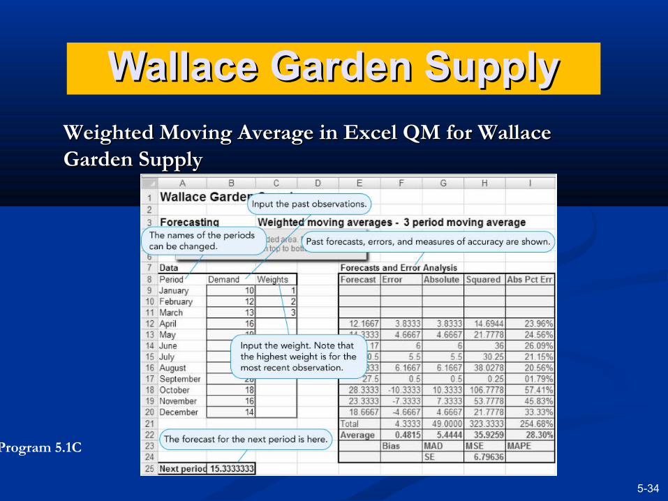
Wallace Garden SupplyWallace Garden Supply
Program 5.1C
Weighted Moving Average in Excel QM for Wallace Weighted Moving Average in Excel QM for Wallace Garden SupplyGarden Supply

5-35
Exponential SmoothingExponential Smoothing
Exponential smoothingExponential smoothing is a type of moving is a type of moving average that is easy to use and requires little average that is easy to use and requires little record keeping of data.record keeping of data.
New forecast = Last period’s forecast+ α(Last period’s actual demand – Last period’s forecast)
Here α is a weight (or smoothing constantsmoothing constant) in which 0≤α≤1.

Exponential SmoothingExponential Smoothing
Mathematically:Mathematically:
)( tttt FYFF −+=+ α1
Where:Ft+1 = new forecast (for time period t + 1)
Ft = pervious forecast (for time period t)
α = smoothing constant (0 ≤ α ≤ 1)Yt = pervious period’s actual demand
The idea is simple – the new estimate is the old estimate plus some fraction of the error in the last period.
5-37
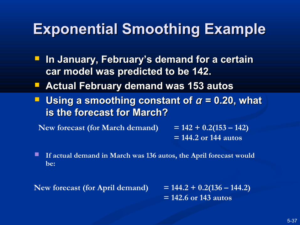
Exponential Smoothing ExampleExponential Smoothing Example
In January, February’s demand for a certain In January, February’s demand for a certain car model was predicted to be 142.car model was predicted to be 142.
Actual February demand was 153 autosActual February demand was 153 autos Using a smoothing constant of Using a smoothing constant of αα = 0.20, what = 0.20, what
is the forecast for March?is the forecast for March?
New forecast (for March demand) = 142 + 0.2(153 – 142)= 144.2 or 144 autos
If actual demand in March was 136 autos, the April forecast would be:
New forecast (for April demand) = 144.2 + 0.2(136 – 144.2)= 142.6 or 143 autos

5-38
Selecting the Smoothing ConstantSelecting the Smoothing Constant
Selecting the appropriate value for α is key to obtaining a good forecast.
The objective is always to generate an accurate forecast.
The general approach is to develop trial forecasts with different values of α and select the α that results in the lowest MAD.

5-39
Exponential SmoothingExponential Smoothing
QUARTER
ACTUAL TONNAGE
UNLOADEDFORECAST
USING α =0.10FORECAST
USING α =0.50
1 180 175 175
2 168 175.5 = 175.00 + 0.10(180 – 175) 177.5
3 159 174.75 = 175.50 + 0.10(168 – 175.50) 172.75
4 175 173.18 = 174.75 + 0.10(159 – 174.75) 165.88
5 190 173.36 = 173.18 + 0.10(175 – 173.18) 170.44
6 205 175.02 = 173.36 + 0.10(190 – 173.36) 180.22
7 180 178.02 = 175.02 + 0.10(205 – 175.02) 192.61
8 182 178.22 = 178.02 + 0.10(180 – 178.02) 186.30
9 ? 178.60 = 178.22 + 0.10(182 – 178.22) 184.15
Table 5.5
Port of Baltimore Exponential Smoothing Forecast for α=0.1 and α=0.5.
5-40
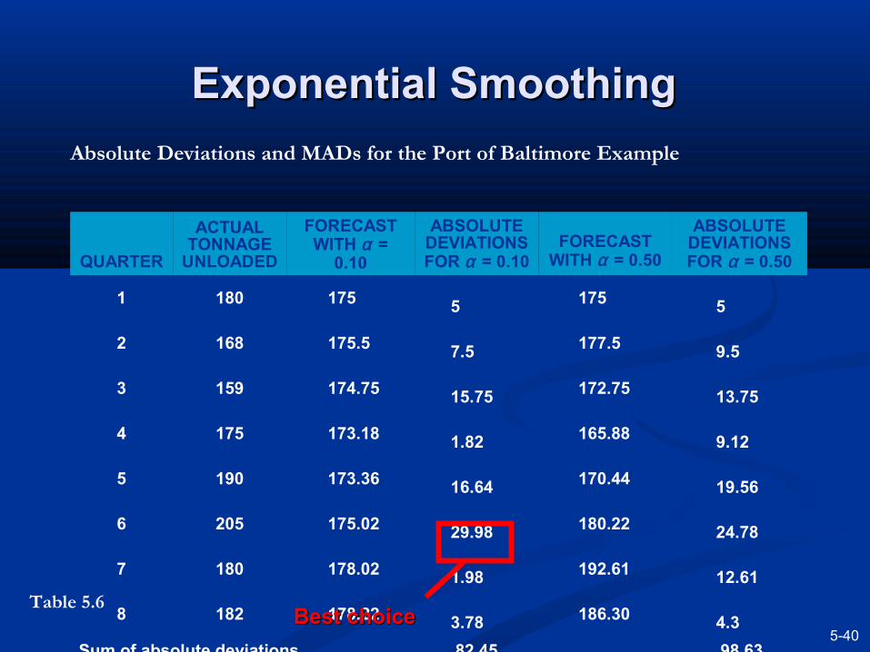
Exponential SmoothingExponential Smoothing
QUARTER
ACTUAL TONNAGE
UNLOADED
FORECAST WITH α =
0.10
ABSOLUTEDEVIATIONS FOR α = 0.10
FORECAST WITH α = 0.50
ABSOLUTEDEVIATIONS FOR α = 0.50
1 180 175 5…..175 5….
2 168 175.5 7.5.. 177.5 9.5..
3 159 174.75 15.75 172.75 13.75
4 175 173.18 1.82 165.88 9.12
5 190 173.36 16.64 170.44 19.56
6 205 175.02 29.98 180.22 24.78
7 180 178.02 1.98 192.61 12.61
8 182 178.22 3.78 186.30 4.3..
Sum of absolute deviations 82.45 98.63
MAD =Σ|deviations|
= 10.31 MAD = 12.33n
Table 5.6Best choiceBest choice
Absolute Deviations and MADs for the Port of Baltimore Example

5-41
Port of Baltimore Exponential Port of Baltimore Exponential Smoothing Example in Excel QMSmoothing Example in Excel QM
Program 5.2

5-42
Exponential Smoothing with Exponential Smoothing with Trend AdjustmentTrend Adjustment
Like all averaging techniques, exponential Like all averaging techniques, exponential smoothing does not respond to trends.smoothing does not respond to trends.
A more complex model can be used that A more complex model can be used that adjusts for trends.adjusts for trends.
The basic approach is to develop an The basic approach is to develop an exponential smoothing forecast, and then exponential smoothing forecast, and then adjust it for the trend.adjust it for the trend.
Forecast including trend (FITt+1) = Smoothed forecast (Ft+1)+ Smoothed Trend (Tt+1)

5-43
Exponential Smoothing with Exponential Smoothing with Trend AdjustmentTrend Adjustment
The equation for the trend correction uses a new The equation for the trend correction uses a new smoothing constant smoothing constant ββ . .
TTtt must be given or estimated. T must be given or estimated. T t+1t+1 is computed by: is computed by:
)()1( 11 tttt FITFTT −+−= ++ ββwhere
Tt = smoothed trend for time period t
Ft = smoothed forecast for time period t
FITt = forecast including trend for time period t
α =smoothing constant for forecastsβ = smoothing constant for trend

5-44
Selecting a Smoothing ConstantSelecting a Smoothing Constant
As with exponential smoothing, a high value of β makes the forecast more responsive to changes in trend.
A low value of β gives less weight to the recent trend and tends to smooth out the trend.
Values are generally selected using a trial-and-error approach based on the value of the MAD for different values of β .

Midwestern ManufacturingMidwestern Manufacturing Midwest Manufacturing has a demand for electrical generators from 2004
– 2010 as given in the table below. To forecast demand, Midwest assumes:
F1 is perfect. T1 = 0. α = 0.3 β = 0.4.
YEAR ELECTRICAL GENERATORS SOLD
2004 74
2005 79
2006 80
2007 90
2008 105
2009 142
2010 122Table 5.7
5-46
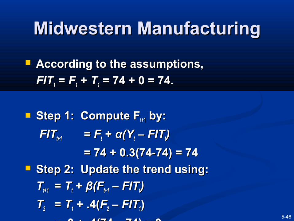
Midwestern ManufacturingMidwestern Manufacturing
According to the assumptions,According to the assumptions,
FITFIT11 = = FF11 + + TT11 = 74 + 0 = 74. = 74 + 0 = 74.
Step 1: Compute FStep 1: Compute F t+1t+1 by: by:
FITFITt+1t+1 = F= Ftt + + αα(Y(Ytt – FIT – FITtt) )
= 74 + 0.3(74-74) = 74= 74 + 0.3(74-74) = 74 Step 2: Update the trend using:Step 2: Update the trend using:
TTt+1t+1 = T= Ttt + + ββ(F(Ft+1t+1 – FIT – FITtt))
TT22 = = TT11 + .4( + .4(FF22 – FIT – FIT11))
= 0 + .4(74 – 74) = 0= 0 + .4(74 – 74) = 0
5-47
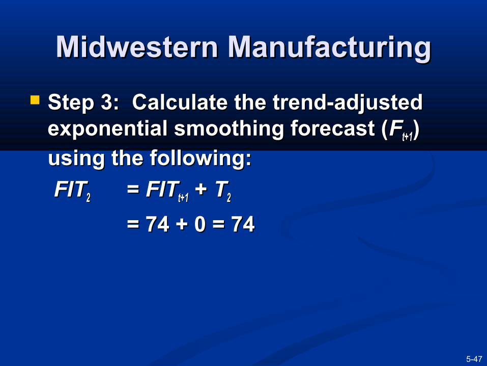
Midwestern ManufacturingMidwestern Manufacturing
Step 3: Calculate the trend-adjusted Step 3: Calculate the trend-adjusted exponential smoothing forecast (exponential smoothing forecast (FFt+1t+1) )
using the following:using the following:
FITFIT22 = FIT= FITt+1t+1 + T + T22
= 74 + 0 = 74= 74 + 0 = 74
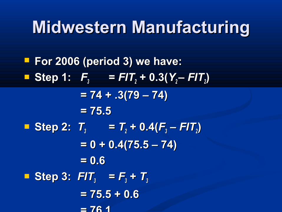
Midwestern ManufacturingMidwestern Manufacturing
For 2006 (period 3) we have:For 2006 (period 3) we have: Step 1:Step 1: FF33 = FIT= FIT22 + 0.3(+ 0.3(YY2 2 – FIT– FIT22))
= 74 + .3(79 – 74)= 74 + .3(79 – 74)
= 75.5= 75.5 Step 2: Step 2: TT33 = T= T22 + 0.4(+ 0.4(FF33 – FIT – FIT22) )
= 0 + 0.4(75.5 – 74)= 0 + 0.4(75.5 – 74)
= 0.6= 0.6 Step 3: Step 3: FITFIT33 = F= F33 + T + T33
= 75.5 + 0.6= 75.5 + 0.6
= 76.1= 76.1

5-49
Midwestern Manufacturing Exponential Midwestern Manufacturing Exponential Smoothing with Trend ForecastsSmoothing with Trend Forecasts
Table 5.8
Time (t)
Demand (Yt)
FITt+1 = Ft + 0.3(Yt– FITt) Tt+1 = Tt + 0.4(Ft+1 – FITt) FITt+1 = Ft+1 + Tt+1
1 74 74 0 74
2 79 74=74+0.3(74-74) 0 = 0+0.4(74-74) 74 = 74+0
3 80 75.5=74+0.3(79-74) 0.6 = 0+0.4(75.5-74) 76.1 = 75.5+0.6
4 90 77.270=76.1+0.3(80-76.1) 1.068 = 0.6+0.4(77.27-76.1) 78.338 = 77.270+1.068
5 105 81.837=78.338+0.3(90-78.338)
2.468 = 1.068+0.4(81.837-78.338)
84.305 = 81.837+2.468
6 142 90.514=84.305+0.3(105-84.305)
4.952 = 2.468+0.4(90.514-84.305)
95.466 = 90.514+4.952
7 122 109.426=95.466+0.3(142-95.466)
10.536 = 4.952+0.4(109.426-95.466)
119.962 = 109.426+10.536
8 120.573=119.962+0.3(122-119.962)
10.780 = 10.536+0.4(120.573-
119.962)
131.353 = 120.573+10.780

5-50
Midwestern ManufacturingMidwestern Manufacturing
Program 5.3
Midwestern Manufacturing Trend-Adjusted Exponential Smoothing in Excel QM
5-51
Trend Projections
Trend projection fits a trend line to a series of historical data points.
The line is projected into the future for medium- to long-range forecasts.
Several trend equations can be developed based on exponential or quadratic models.
The simplest is a linear model developed using regression analysis.

5-52
Trend Projection
The mathematical form is
XbbY 10 +=ˆ
Where= predicted value
b0 = interceptb1 = slope of the lineX = time period (i.e., X = 1, 2, 3, …, n)
Y

5-53
Midwestern ManufacturingMidwestern Manufacturing
Program 5.4A
Excel Input Screen for Midwestern Manufacturing Trend Line

5-54
Midwestern ManufacturingMidwestern Manufacturing
Program 5.4B
Excel Output for Midwestern Manufacturing Trend Line

5-55
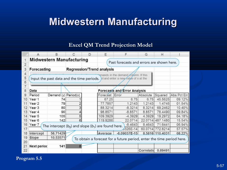
Midwestern Manufacturing Midwestern Manufacturing Company ExampleCompany Example
The forecast equation is
XY 54107156 ..ˆ +=
To project demand for 2011, we use the coding system to define X = 8
(sales in 2011) = 56.71 + 10.54(8)= 141.03, or 141 generators
Likewise for X = 9
(sales in 2012) = 56.71 + 10.54(9)= 151.57, or 152 generators

5-56
Midwestern ManufacturingMidwestern Manufacturing
Figure 5.4
Electrical Generators and the Computed Trend Line
5-57
Midwestern ManufacturingMidwestern Manufacturing
Program 5.5
Excel QM Trend Projection Model
Seasonal VariationsSeasonal Variations
Recurring variations over time may Recurring variations over time may indicate the need for seasonal indicate the need for seasonal adjustments in the trend line.adjustments in the trend line.
A seasonal index indicates how a A seasonal index indicates how a particular season compares with an particular season compares with an average season.average season.
When no trend is present, the seasonal When no trend is present, the seasonal index can be found by dividing the index can be found by dividing the average value for a particular season by average value for a particular season by the average of all the data.the average of all the data.
5-59
Eichler SuppliesEichler Supplies
Eichler Supplies sells telephone Eichler Supplies sells telephone answering machines.answering machines.
Sales data for the past two years has Sales data for the past two years has been collected for one particular model.been collected for one particular model.
The firm wants to create a forecast that The firm wants to create a forecast that includes seasonality.includes seasonality.
5-60
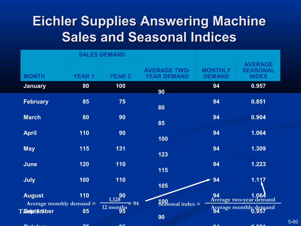
Eichler Supplies Answering Machine Eichler Supplies Answering Machine Sales and Seasonal IndicesSales and Seasonal Indices
MONTH
SALES DEMAND
AVERAGE TWO- YEAR DEMAND
MONTHLY DEMAND
AVERAGE SEASONAL
INDEXYEAR 1 YEAR 2
January 80 10090
94 0.957
February 85 7580
94 0.851
March 80 9085
94 0.904
April 110 90100
94 1.064
May 115 131123
94 1.309
June 120 110115
94 1.223
July 100 110105
94 1.117
August 110 90100
94 1.064
September 85 9590
94 0.957
October 75 8580
94 0.851
November 85 7580
94 0.851
December 80 8080
94 0.851
Total average demand = 1,128
Seasonal index =Average two-year demandAverage monthly demand
Average monthly demand = = 941,128
12 monthsTable 5.9
5-61
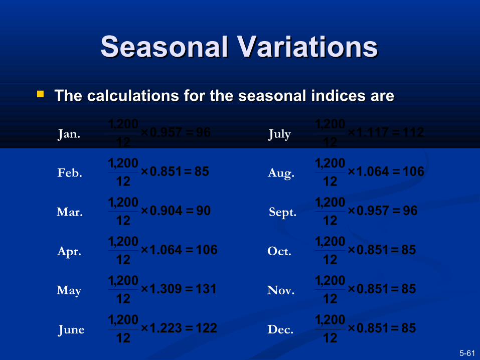
Seasonal VariationsSeasonal Variations
The calculations for the seasonal indices areThe calculations for the seasonal indices are
Jan. July969570122001 =× .,
1121171122001 =× .,
Feb. Aug.858510122001 =× .,
1060641122001 =× .,
Mar. Sept.909040122001 =× .,
969570122001 =× .,
Apr. Oct.1060641122001 =× .,
858510122001 =× .,
May Nov.1313091122001 =× .,
858510122001 =× .,
June Dec.1222231122001 =× .,
858510122001 =× .,
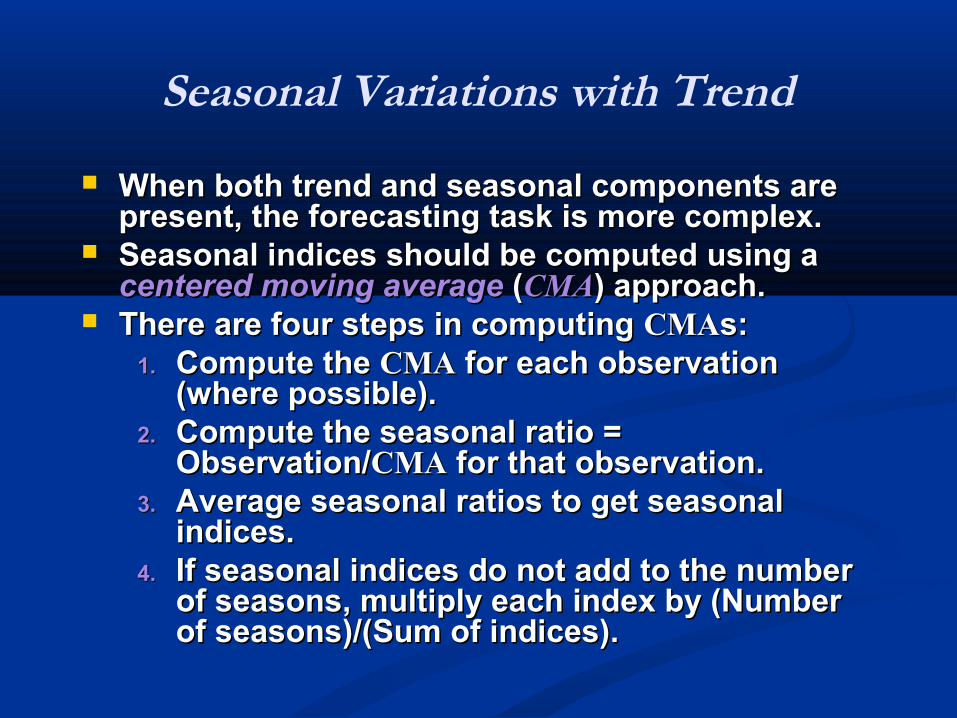
Seasonal Variations with Trend
When both trend and seasonal components are When both trend and seasonal components are present, the forecasting task is more complex.present, the forecasting task is more complex.
Seasonal indices should be computed using a Seasonal indices should be computed using a centered moving averagecentered moving average ( (CMACMA) approach.) approach.
There are four steps in computing There are four steps in computing CMACMAs:s:1.1. Compute the Compute the CMACMA for each observation for each observation
(where possible).(where possible).2.2. Compute the seasonal ratio = Compute the seasonal ratio =
Observation/Observation/CMACMA for that observation. for that observation.3.3. Average seasonal ratios to get seasonal Average seasonal ratios to get seasonal
indices.indices.4.4. If seasonal indices do not add to the number If seasonal indices do not add to the number
of seasons, multiply each index by (Number of seasons, multiply each index by (Number of seasons)/(Sum of indices).of seasons)/(Sum of indices).
5-63
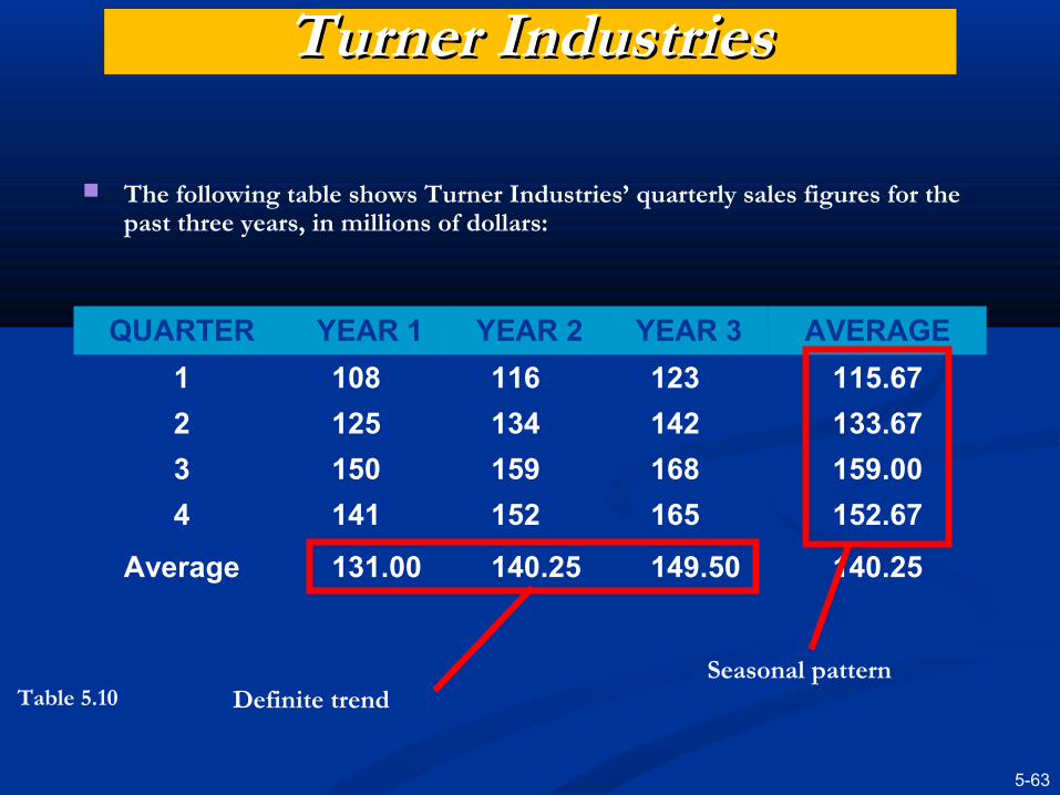
Turner IndustriesTurner Industries
The following table shows Turner Industries’ quarterly sales figures for the past three years, in millions of dollars:
QUARTER YEAR 1 YEAR 2 YEAR 3 AVERAGE
1 108 116 123 115.67
2 125 134 142 133.67
3 150 159 168 159.00
4 141 152 165 152.67
Average 131.00 140.25 149.50 140.25
Table 5.10 Definite trendSeasonal pattern

5-64
Turner Industries
To calculate the CMA for quarter 3 of year 1 we compare the actual sales with an average quarter centered on that time period.
We will use 1.5 quarters before quarter 3 and 1.5 quarters after quarter 3 – that is we take quarters 2, 3, and 4 and one half of quarters 1, year 1 and quarter 1, year 2.
CMA(q3, y1) = = 132.000.5(108) + 125 + 150 + 141 + 0.5(116)
4

5-65
Turner Industries
Compare the actual sales in quarter 3 to the CMA to find the seasonal ratio:
13611321503 quarter in Sales
ratio Seasonal .CMA
===
5-66
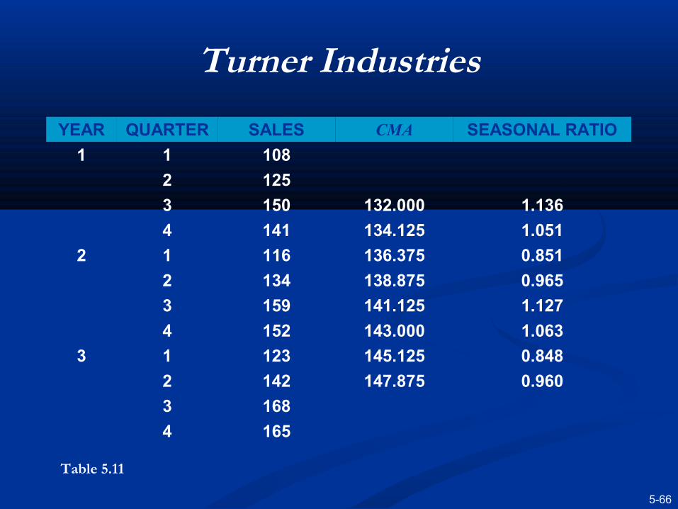
Turner Industries
YEAR QUARTER SALES CMA SEASONAL RATIO
1 1 108
2 125
3 150 132.000 1.136
4 141 134.125 1.051
2 1 116 136.375 0.851
2 134 138.875 0.965
3 159 141.125 1.127
4 152 143.000 1.063
3 1 123 145.125 0.848
2 142 147.875 0.960
3 168
4 165
Table 5.11

5-67
Turner Industries
There are two seasonal ratios for each quarter so these are averaged to get the seasonal index:
Index for quarter 1 = I1 = (0.851 + 0.848)/2 = 0.85
Index for quarter 2 = I2 = (0.965 + 0.960)/2 = 0.96
Index for quarter 3 = I3 = (1.136 + 1.127)/2 = 1.13
Index for quarter 4 = I4 = (1.051 + 1.063)/2 = 1.06
5-68
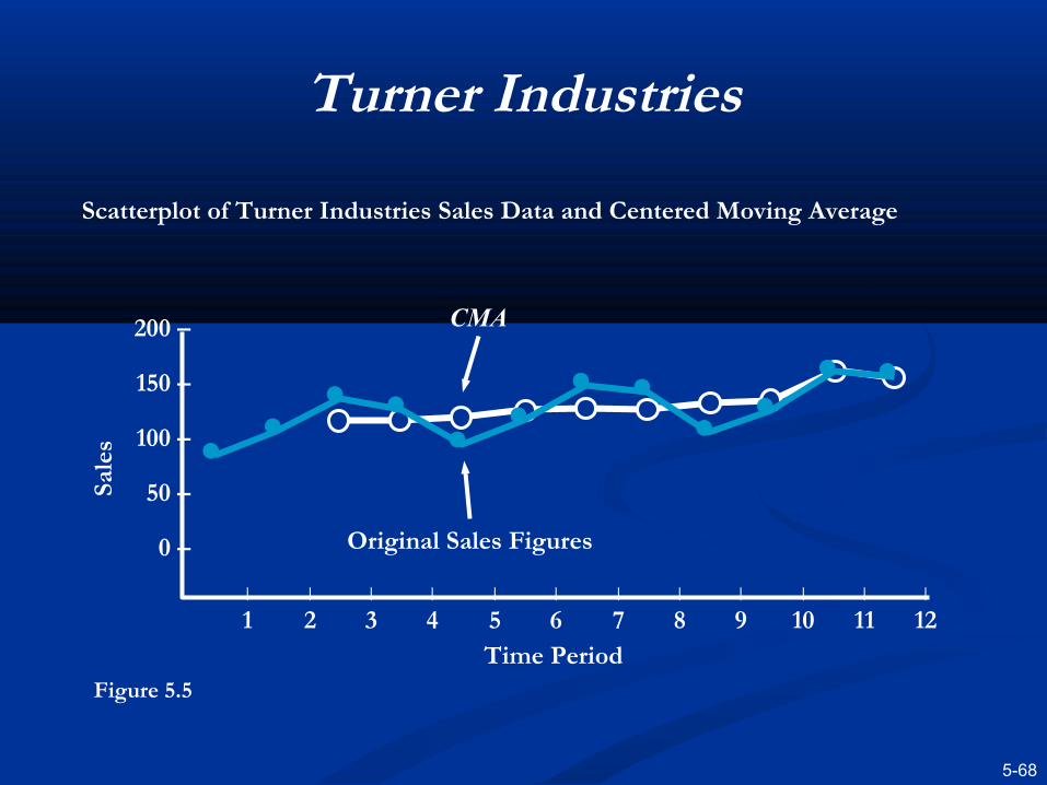
Turner Industries
Scatterplot of Turner Industries Sales Data and Centered Moving Average
CMA
Original Sales Figures
200 –
150 –
100 –
50 –
0 –
Sale
s
| | | | | | | | | | | |
1 2 3 4 5 6 7 8 9 10 11 12Time Period
Figure 5.5
5-69
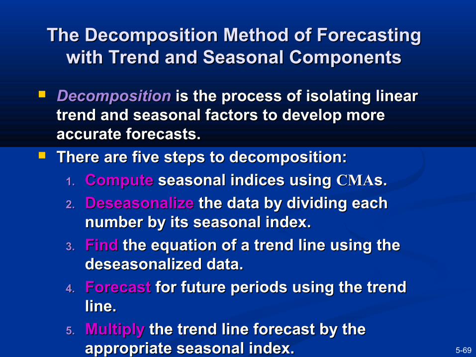
The Decomposition Method of Forecasting The Decomposition Method of Forecasting with Trend and Seasonal Componentswith Trend and Seasonal Components
DecompositionDecomposition is the process of isolating linear is the process of isolating linear trend and seasonal factors to develop more trend and seasonal factors to develop more accurate forecasts.accurate forecasts.
There are five steps to decomposition:There are five steps to decomposition:
1.1. ComputeCompute seasonal indices using seasonal indices using CMACMAs.s.
2.2. Deseasonalize Deseasonalize the data by dividing each the data by dividing each number by its seasonal index.number by its seasonal index.
3.3. FindFind the equation of a trend line using the the equation of a trend line using the deseasonalized data.deseasonalized data.
4.4. ForecastForecast for future periods using the trend for future periods using the trend line.line.
5.5. MultiplyMultiply the trend line forecast by the the trend line forecast by the appropriate seasonal index.appropriate seasonal index.

5-70
Deseasonalized Data for Turner Deseasonalized Data for Turner IndustriesIndustries
Find a trend line using the deseasonalized data:
b1 = 2.34 b0 = 124.78
Develop a forecast using this trend and multiply the forecast by the appropriate seasonal index.
Y = 124.78 + 2.34X= 124.78 + 2.34(13)= 155.2 (forecast before adjustment for seasonality)
Y x I1 = 155.2 x 0.85 = 131.92

5-71
Deseasonalized Data for Turner Deseasonalized Data for Turner IndustriesIndustries
SALES ($1,000,000s)
SEASONAL INDEX
DESEASONALIZED SALES ($1,000,000s)
108 0.85 127.059
125 0.96 130.208
150 1.13 132.743
141 1.06 133.019
116 0.85 136.471
134 0.96 139.583
159 1.13 140.708
152 1.06 143.396
123 0.85 144.706
142 0.96 147.917
168 1.13 148.673
165 1.06 155.660
Table 5.12
5-72
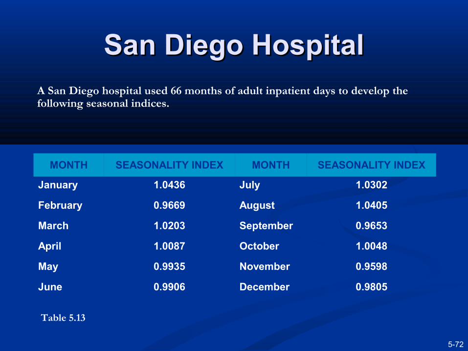
San Diego HospitalSan Diego HospitalA San Diego hospital used 66 months of adult inpatient days to develop the following seasonal indices.
MONTH SEASONALITY INDEX MONTH SEASONALITY INDEX
January 1.0436 July 1.0302
February 0.9669 August 1.0405
March 1.0203 September 0.9653
April 1.0087 October 1.0048
May 0.9935 November 0.9598
June 0.9906 December 0.9805
Table 5.13
5-73
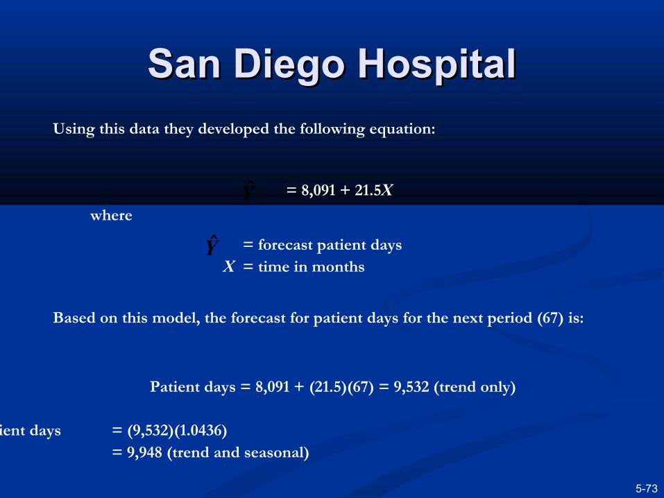
San Diego HospitalSan Diego HospitalUsing this data they developed the following equation:
Y = 8,091 + 21.5X
where
Y = forecast patient daysX = time in months
Based on this model, the forecast for patient days for the next period (67) is:
Patient days = 8,091 + (21.5)(67) = 9,532 (trend only)
Patient days = (9,532)(1.0436) = 9,948 (trend and seasonal)
5-74
San Diego HospitalSan Diego Hospital
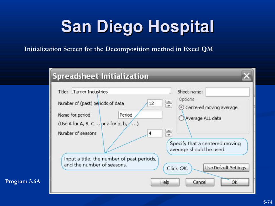
Program 5.6A
Initialization Screen for the Decomposition method in Excel QM

5-75
San Diego HospitalSan Diego Hospital
Program 5.6B
Turner Industries Forecast Using the Decomposition Method in Excel QM

5-76
Using Regression with Trend Using Regression with Trend and Seasonal Componentsand Seasonal Components
Multiple regressionMultiple regression can be used to forecast both can be used to forecast both trend and seasonal components in a time series.trend and seasonal components in a time series. One independent variable is time.One independent variable is time. Dummy independent variables are used to represent the Dummy independent variables are used to represent the
seasons.seasons.
The model is an additive decomposition model:The model is an additive decomposition model:
where X1 = time periodX2 = 1 if quarter 2, 0 otherwiseX3 = 1 if quarter 3, 0 otherwiseX4 = 1 if quarter 4, 0 otherwise
44332211 XbXbXbXbaY ++++=ˆ

5-77
Regression with Trend and Regression with Trend and Seasonal ComponentsSeasonal Components
Program 5.7A
Excel Input for the Turner Industries Example Using Multiple Regression
Using Regression with Trend Using Regression with Trend and Seasonal Componentsand Seasonal Components
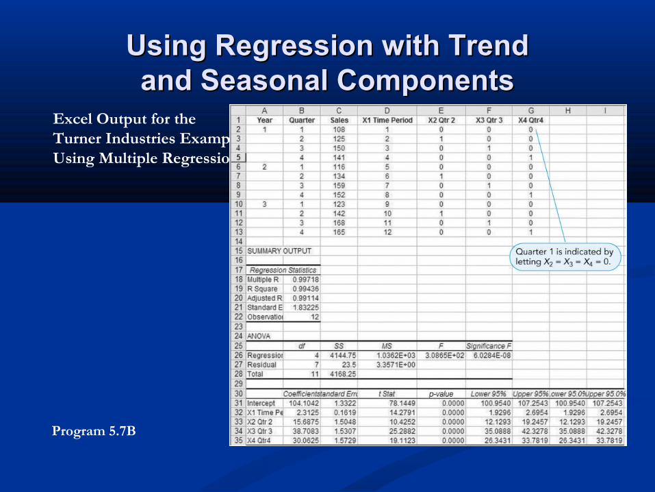
Program 5.7B
Excel Output for the Turner Industries Example Using Multiple Regression
5-79
Using Regression with Trend Using Regression with Trend and Seasonal Componentsand Seasonal Components
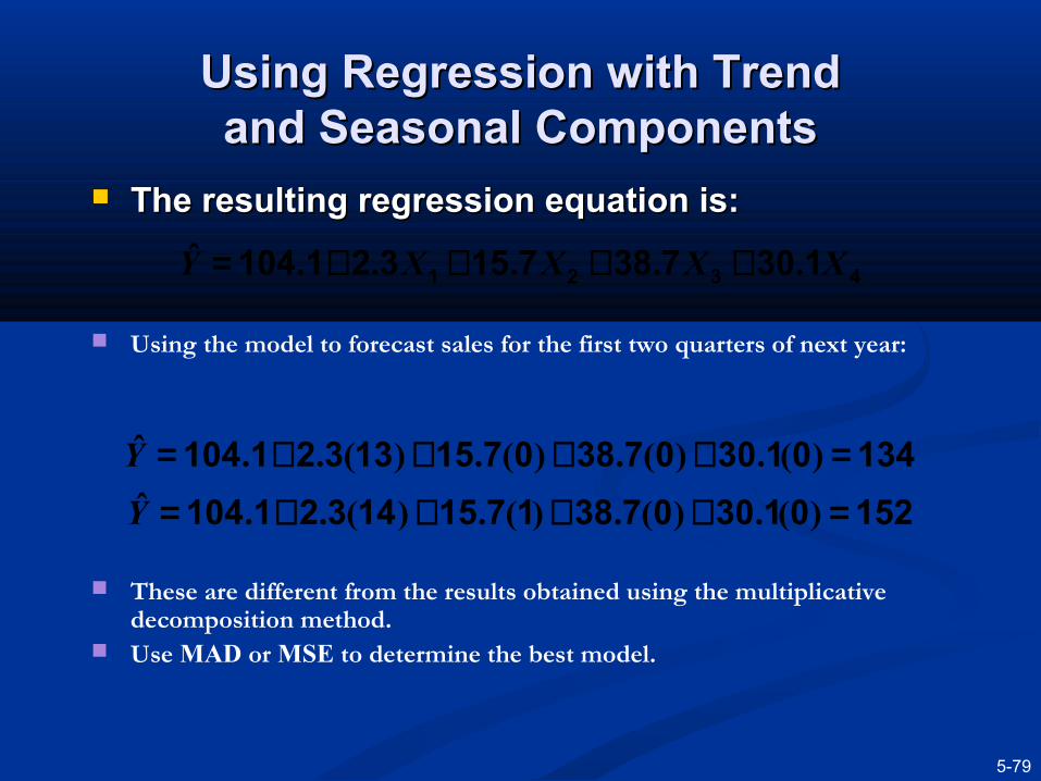
The resulting regression equation is:The resulting regression equation is:
4321 130738715321104 XXXXY .....ˆ ++++=
Using the model to forecast sales for the first two quarters of next year:
These are different from the results obtained using the multiplicative decomposition method.
Use MAD or MSE to determine the best model.
13401300738071513321104 =++++= )(.)(.)(.)(..Y
15201300738171514321104 =++++= )(.)(.)(.)(..Y
5-80
Monitoring and Controlling ForecastsMonitoring and Controlling Forecasts
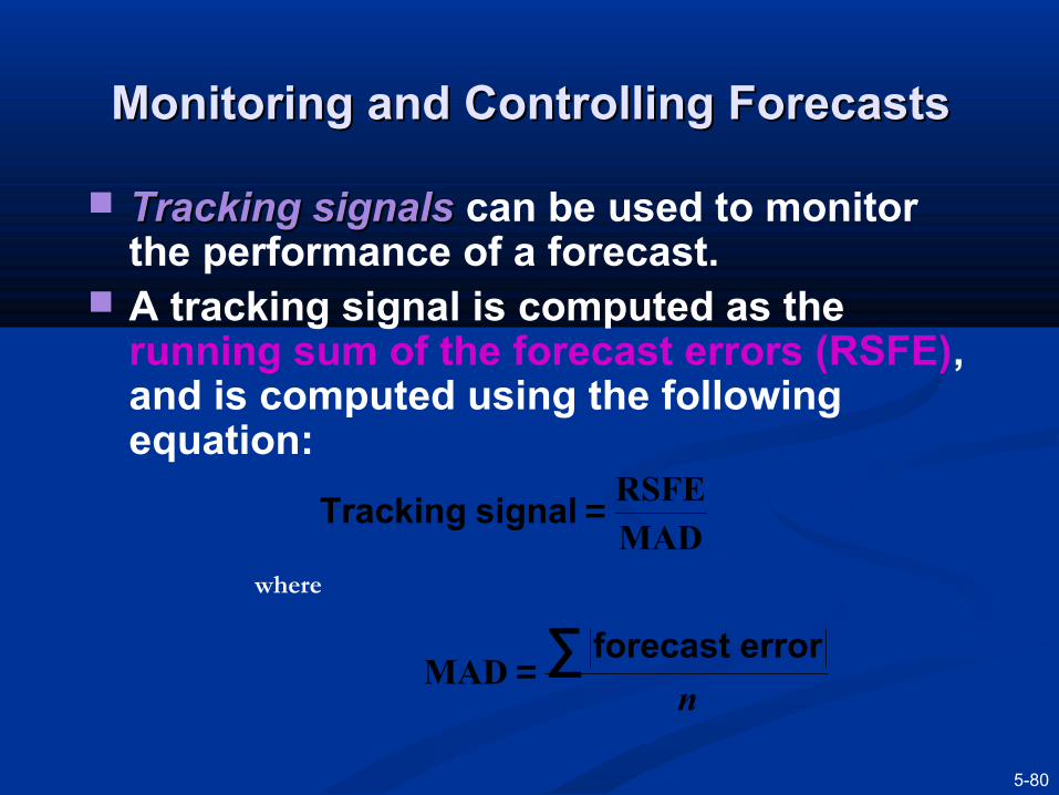
Tracking signalsTracking signals can be used to monitor the performance of a forecast.
A tracking signal is computed as the running sum of the forecast errors (RSFE), and is computed using the following equation:
MADRSFE=signal Tracking
n∑=
errorforecast MAD
where

5-81
Monitoring and Controlling ForecastsMonitoring and Controlling Forecasts
Acceptable Range
Signal Tripped
Upper Control Limit
Lower Control Limit
0 MADs
+
–
TimeFigure 5.6
Tracking Signal
Plot of Tracking Signals

5-82
Monitoring and Controlling ForecastsMonitoring and Controlling Forecasts
Positive tracking signals indicate demand is greater than forecast. Negative tracking signals indicate demand is less than forecast. Some variation is expected, but a good forecast will have about as much
positive error as negative error. Problems are indicated when the signal trips either the upper or lower
predetermined limits. This indicates there has been an unacceptable amount of variation. Limits should be reasonable and may vary from item to item.
Copyright ©2012 Pearson Education, Inc. publishing as
Prentice Hall5-83
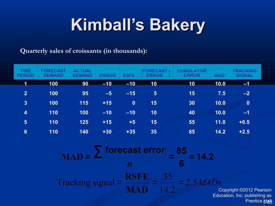
Kimball’s BakeryKimball’s BakeryQuarterly sales of croissants (in thousands):
TIME PERIOD
FORECAST DEMAND
ACTUAL DEMAND ERROR RSFE
|FORECAST || ERROR |
CUMULATIVE ERROR MAD
TRACKING SIGNAL
1 100 90 –10 –10 10 10 10.0 –1
2 100 95 –5 –15 5 15 7.5 –2
3 100 115 +15 0 15 30 10.0 0
4 110 100 –10 –10 10 40 10.0 –1
5 110 125 +15 +5 15 55 11.0 +0.5
6 110 140 +30 +35 35 85 14.2 +2.5
2146
85errorforecast .MAD === ∑
n
MADs5.22.14
35signal Tracking ===
MAD
RSFE
Adaptive SmoothingAdaptive Smoothing
Adaptive smoothingAdaptive smoothing is the computer is the computer monitoring of tracking signals and self-monitoring of tracking signals and self-adjustment if a limit is tripped.adjustment if a limit is tripped.
In exponential smoothing, the values of In exponential smoothing, the values of αα and and ββ are adjusted when the computer are adjusted when the computer detects an excessive amount of variation.detects an excessive amount of variation.

TutorialTutorial
Lab Practical : Spreadsheet Lab Practical : Spreadsheet
1 - 85
Further ReadingFurther Reading
Render, B., Stair Jr.,R.M. & Hanna, M.E. (2013) Quantitative Analysis for Management, Pearson, 11th Edition
Waters, Donald (2007) Quantitative Methods for Business, Prentice Hall, 4 th Edition.
Anderson D, Sweeney D, & Williams T. (2006) Quantitative Methods For Business Thompson Higher Education, 10th Ed.

QUESTIONS?QUESTIONS?