bci mardie salt project - epa wa

rpsgroup.com

BCI MARDIE SALT PROJECT Coastal Inundation Studies

MAW0616J.006

BCI Mardie Salt Project

Rev 3

29 November 2019

REPORT

MAW0616J.006 | BCI Mardie Salt Project | Rev 3 | 29 November 2019 rpsgroup.com Page i

Document status

Version Purpose of document Authored by Reviewed by Approved by Review date

Rev 0 Issued for client review S. Langtry R. Alexander D. Wright 07/06/2018

Rev 1 Issued for client review S. Langtry R. Alexander D. Wright 21/06/2018

Rev 2 Issued with additional details S. Langtry R. Alexander D. Wright 24/04/2019

Rev 3 Issued for revised pond details S. Langtry R. Alexander D. Wright 29/11/2019

Approval for issue

David Wright 29 November 2019

This report was prepared by RPS within the terms of RPS’ engagement with its client and in direct response to a scope of services. This report is supplied for the sole and specific purpose for use by RPS’ client. The report does not account for any changes relating the subject matter of the report, or any legislative or regulatory changes that have occurred since the report was produced and that may affect the report. RPS does not accept any responsibility or liability for loss whatsoever to any third party caused by, related to or arising out of any use or reliance on the report.

Prepared by: Prepared for:

RPS BCI MINERALS PTY LTD

Scott Langtry Principal Scientist

Neil Dixon Manager Approvals

Level 2, 27-31 Troode Street West Perth WA 6005

Level 2, 1 Altona Sreet West Perth WA 6005

T +61 8 9211 1111 E [email protected]

T +61 8 6311 3400 E [email protected]

REPORT

MAW0616J.006 | BCI Mardie Salt Project | Rev 3 | 29 November 2019 rpsgroup.com Page ii

Contents

1 BACKGROUND ....................................................................................................................................... 1

2 DESCRIPTION OF THE MODEL ............................................................................................................. 3 2.1 Model code and grid set up ............................................................................................................ 3 2.2 Forcing conditions provided to the model simulations ................................................................... 1 2.3 Representation of the pond walls ................................................................................................... 4

3 RESULTS OF THE SIMULATIONS ......................................................................................................... 6 3.1 Natural patterns of inundation ........................................................................................................ 6 3.2 Effect of the pond walls on inundation .........................................................................................11 3.3 Effect of the pond walls on inundation of the algal mats and mangroves ....................................20 3.4 Effect of the pond walls on inundation with sea level rise ............................................................25

4 APPENDIX .............................................................................................................................................34 4.1 Inundation frequency data ............................................................................................................34

Tables

Table 4-1 Base case in algal mats ...............................................................................................................35 Table 4-2 Pond case in algal mats ...............................................................................................................36 Table 4-3 Comparison of percentile distribution of water depth (Pond Case - Base Case) in algal

mats ..............................................................................................................................................37 Table 4-4 Base case with 0.9 m sea level rise in algal mats ........................................................................38 Table 4-5 Pond case with 0.9 m sea level rise in algal mats .......................................................................39 Table 4-6 Comparison of percentile distribution of water depth (Pond Case - Base Case) in algal

mats with 0.9 m sea level rise ......................................................................................................40 Table 4-7 Base case in mangroves ..............................................................................................................41 Table 4-8 Pond case in mangroves ..............................................................................................................42 Table 4-9 Comparison of percentile distribution of water depth (Pond Case - Base Case) in

mangroves ....................................................................................................................................43 Table 4-10 Base case with 0.9 m sea level rise in mangroves ......................................................................44 Table 4-11 Pond case with 0.9 m sea level rise in mangroves ......................................................................45 Table 4-12 Comparison of percentile distribution of water depth (Pond Case - Base Case) in

mangroves with 0.9 m sea level rise ............................................................................................46

Figures

Figure 1.1 Location of the Mardie project area. The upper panel shows the regional setting of the project area on the North West Shelf of Australia. The lower panel shows a satellite image captured at around mid-tide level, showing the extensive creek network fronting clay pans. ....................................................................................................................................... 2

Figure 2.1 Domain of the regional grid used to calculate forcing conditions at the open boundaries of the inundation grid .......................................................................................................................... 4

Figure 2.2 Details of the inundation grid applying depth coding that emphasises the creeks, offshore mudbanks and channel details. The connection to the offshore grid is also illustrated. ................ 6

Figure 2.3 Details of the inundation grid applying depth coding that emphasises variations in elevation over the inundated area (> 0.5 m above MSL). .............................................................. 7

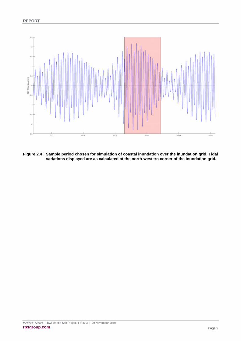
Figure 2.4 Sample period chosen for simulation of coastal inundation over the inundation grid. Tidal variations displayed are as calculated at the north-western corner of the inundation grid. ........... 2

REPORT

MAW0616J.006 | BCI Mardie Salt Project | Rev 3 | 29 November 2019 rpsgroup.com Page iii

Figure 2.5 Comparison of tidal measurements made in two creeks with tidal elevations calculated by the nested model configuration. The yellow crosses on the maps show the measurement locations. ........................................................................................................................................ 3

Figure 2.6 Layout of the pond walls that was applied in the model to test effects on coastal inundation. ...................................................................................................................................... 5

Figure 3.1 Calculations for water depth over the project area as the tide is peaking during a high spring tide (2.1 m MSL Peak). Note the timing of the snapshots has been varied to highlight the more rapid changes and is marked at the top of each panel. ................................... 7

Figure 3.2 Calculations for water depth over the project area as the tide is lowering after the same high spring tide (2.1 m MSL Peak) shown in Figure 2.5. ............................................................... 9

Figure 3.3 Calculations for water depth over the project area as the tide is rising to a spring tide (1.8 m MSL) for the Pond Case. ..........................................................................................................12

Figure 3.4 Calculations for water depth over the project area as the tide is rising to a high spring tide (2.2 m MSL) for the Pond Case. Times correspond to images in Figure 3.1 ..............................13

Figure 3.5 Calculations for increased water depth as the tide rises to a high spring tide (2.2 m MSL) with the pond walls in place. ........................................................................................................15

Figure 3.6 Calculations for decreased water depth as the tide falls after a high spring tide (2.2 m MSL) with the pond walls in place. ...............................................................................................17

Figure 3.7 Comparison of the frequency of different water depths between the Pond Case and Base Case at locations near the walls. The Y-axis shows water depth in cm. The X-axis shows the percentile exceedance (e.g. the 90th percentile would be exceeded 10% of the time; the 60th percentile would be exceeded 40% of the time). Line colours correspond to X marks on the map. Lines with crosses represent the Pond Case. ...............................................19

Figure 3.8 Inundation frequencies calculated over the simulation period for locations in the algal mat zone, derived from the Base Case simulation. Line styles and colours refer to locations shown in the inset. .......................................................................................................................21

Figure 3.9 Inundation frequencies calculated over the simulation period for locations in the algal mat zone, derived from the Pond Case simulation. Line styles and colours refer to locations shown in the inset. .......................................................................................................................22

Figure 3.10 Inundation frequencies calculated over the simulation period for locations in the mangrove zone, derived from the Base Case simulation. Line styles and colours refer to locations shown in the inset. ........................................................................................................23

Figure 3.11 Inundation frequencies calculated over the simulation period for locations in the mangrove zone, derived from the Pond Case simulation. Line styles and colours refer to locations shown in the inset. ........................................................................................................24

Figure 3.12 Calculation of water depth over the project area as the tide rises to a tidal level of 2.9 m MSL ..............................................................................................................................................26

Figure 3.13 Calculation of water depth over the project area as the tide rises to a tidal level of 2.9 m MSL, with the pond walls in place ................................................................................................28

Figure 3.14 Inundation frequencies calculated over the simulation period for locations in the algal mat zone, derived from the Base Case simulation with an additional 0.9 m of sea level rise. Line styles and colours refer to locations shown in the inset. ......................................................30

Figure 3.15 Inundation frequencies calculated over the simulation period for locations in the algal mat zone, derived from the Pond Case simulation with an additional 0.9 m of sea level rise. Line styles and colours refer to locations shown in the inset. ......................................................31

Figure 3.16 Inundation frequencies calculated over the simulation period for locations in the mangrove zone, derived from the Base Case simulation with an additional 0.9 m of sea level rise. Line styles and colours refer to locations shown in the inset.......................................32

Figure 3.17 Inundation frequencies calculated over the simulation period for locations in the mangrove zone, derived from the Pond Case simulation with an additional 0.9 m of sea level rise. Line styles and colours refer to locations shown in the inset.......................................33

REPORT

MAW0616J.006 | BCI Mardie Salt Project | Rev 3 | 29 November 2019 rpsgroup.com Page 1

1 BACKGROUND

BC Minerals limited (BCI) is proposing to construct new solar-salt production facilities near Mardie, on the Pilbara Coast of Western Australia (Figure 1.1).

The project would involve construction of a series of linked evaporation ponds over the impermeable soils that occur inshore from the coast. The coast is composed of mud and sand banks in front of relatively flat and highly-eroded land that is penetrated by multiple, highly-branched, creeks that extend up to several kilometres inland. The creeks are lined by mangroves and salt-marsh vegetation and review of satellite images spanning around 13 years (from 2004) indicates that there has been increased colonisation of many of the creeks by mangroves along with increased branching of the creeks over time. Clay pans occur behind the mangrove zone and a portion of the clay pan area is colonised by algae and cyanobacteria that form extensive crusting mats.

The creek systems provide a conduit for seawater to migrate inwards and outwards in response to tidal variations. There is evidence provided by regular satellite records that the land surrounding the creeks is also regularly inundated by the sea in response to tidal fluctuations as well as additional water set-up generated by storms and other oceanographic conditions. It is also believed that the mangroves, salt-marsh and mat-forming algae rely upon unique rates of inundation by the sea to maintain health.

One of the key concerns for the placement of the evaporation ponds and associated development would be the potential for impact of the pond walls on natural water flow and rates of inundation, by the sea, of the mangroves, saltmarsh and algal mats.

RPS was commissioned to develop a coastal inundation model that illustrates the inundation of the existing project area due to tidal variation and then apply that model to test the effect of:

• Placement of the pond walls, based on the layout of external walls proposed for the project at this stage;

• Sea level rise, based on a design level increase of 0.9 m over 100 years.

This technical memo provides basic details of the model configuration and conditions that were modelled as well as results of the modelling assessment.

REPORT


Figure 1.1 Location of the Mardie project area. The upper panel shows the regional setting of the project area on the North West Shelf of Australia. The lower panel shows a satellite image captured at around mid-tide level, showing the extensive creek network fronting clay pans.

REPORT


2 DESCRIPTION OF THE MODEL

2.1 Model code and grid set up

The coastal inundation model was built using the DELFT3D modelling code, originally developed by Deltares in the Netherlands, and since extended by researchers worldwide as an open source hydrodynamic model. The model is designed to simulate hydrodynamic circulation, wave-action, sediment transport and water quality in fluvial, estuarine and coastal environments. The hydrodynamic flow module of this software, DELFT3D Flow, was applied to simulate hydrodynamic flow over a digital elevation model covering the study area and the surrounding portion of the North West Shelf.

Two modelling domains were developed to support the investigation:

A regional model domain was developed over a relatively coarse model grid to calculate the propagation of astronomical tidal waves into the study area. The regional scale model was established over a domain that covered approximately 300 km of the North West Shelf, extending from Onslow to beyond the Dampier Archipelago (Figure 2.1). This domain extended approx. 125 km seaward of the development area with open boundaries extending off the continental shelf and a coastal boundary that extended into the coast bordering the study area.

The larger part of the domain was subdivided into cells that were 2 km x 2 km.

Inputs to the regional model included:

• Bathymetry of the region surrounding the study area;

• Variations in water elevations;

• Definition of the drag imposed by the seabed.

Variations in water levels due to astronomical tides were calculated from a database describing variations in the phase and amplitude of individual tidal constituents over the region at approximately 3 km spacing. This database is calculated from satellite observations over the past 25 years. Water elevations at hourly intervals were calculated from the TPXO8.0 database, which is the most recent iteration of a global model of ocean tides derived from measurements of sea-surface topography by the TOPEX/Poseidon satellite-borne radar altimeters.

REPORT


Figure 2.1 Domain of the regional grid used to calculate forcing conditions at the open boundaries of the inundation grid

REPORT


The regional scale model was operated over a defined period of past time to calculate the propagation of water levels onto the open boundaries of a second grid (inundation grid) that was established over the study area at finer resolution (Figure 2.2 and Figure 2.3) to calculate inundation of water onto and off the land within the development area.

The inundation grid was established over a domain that enclosed the proposed development area and extended 3-5 km offshore from the coast at mean sea level. This domain was subdivided into square cells that each measured 10 m x 10 m, sufficient to calculate variations in water levels over time at 10 m horizontal spacing.

Inputs to the inundation model included:

• A digital elevation grid that defined variation in land heights over the domain (at 10 m x 10 m horizontal resolution);

• Variations in water elevations along the offshore boundary of the inundation grid over time that were calculated by the regional model;

• Definition of the drag imposed by the land.

REPORT


Figure 2.2 Details of the inundation grid applying depth coding that emphasises the creeks, offshore mudbanks and channel details. The connection to the offshore grid is also illustrated.

REPORT


Figure 2.3 Details of the inundation grid applying depth coding that emphasises variations in elevation over the inundated area (> 0.5 m above MSL).

REPORT


2.2 Forcing conditions provided to the model simulations

The study region is constantly subjected to varying water levels, with the major forcing generated by astronomical tidal waves. Additional, less regular, variations are generated by fluctuations in atmospheric pressure, set up due to wave pumping and local anomalies in sea height generated by ocean-scale eddies and ocean currents acting offshore.

Tidal measurements made by BCI within 2 creeks over multiple spring-neap cycles confirmed that tidal fluctuations occur in-phase along the study area but there is a small gradient in the amplitude of the tidal wave that varies with the tidal phase. Highest magnitudes occur towards the north of the Mardie area and tide levels decrease towards the south. Evaluation of time-lapse photography made at 12 creeks distributed along the Mardie project area also revealed variation in the tidal levels required for flooding of the salt pan areas beyond the creeks. The clay pan areas at the northern end of the project area were observed to flood when the tidal level exceeded 1.2 - 1.3 m above MSL (relative to the northern tidal level). In contrast, flooding of the salt pans surrounding creeks towards the south required tidal levels of the order of 1.5 – 1.7 m above MSL. The tidal period of the tidal measurement and time-lapse photography coincided with the annual King Tide levels at the project area and extensive flooding was observed over the salt-pan area at the end of all creeks over the highest tides.

Tidal measurements in the northern creek were evaluated to identify a sample period where tides were rising towards a high spring-tide that exceeded heights that would cause flooding from all creeks. A sample period was selected where high tide ranged from 1.3 m above MSL up to 2.2 m above MSL before receding into a neap period where high tide level reduced to 0.75 m MSL. The sample period spanned 2nd January to 10th January 2018 (Figure 2.4). Review of tidal offset information (e.g. AusCoast VDT) indicates that MSL approximates to the local AHD over the longer term. The exact relationship between MSL and AHD is subject to confirmation for this site and this is a potential source of uncertainty for the model results. However, this difference is typically less than 0.1 m.

To account for the tidal gradient along the study area, the regional hydrodynamic model was operated to calculate variation in tidal propagation onto the coast for the chosen sample period. Validation of the performance of the tidal calculations was provided by the close representation of the tidal variations that were measured in both creeks (Figure 1.6). Note that the tide gauges used for the measurements were placed at locations that dried at low tides. Hence the signal returned from the instruments did not properly record water levels below around 0.7 m below MSL. However, the model was configured to have deeper water at these locations and calculated the full tidal cycle. Nevertheless, the comparisons show that the model closely reproduced the phase and timing of the tidal elevations over the higher tidal phases which were used to force coastal inundation.

REPORT


Figure 2.4 Sample period chosen for simulation of coastal inundation over the inundation grid. Tidal variations displayed are as calculated at the north-western corner of the inundation grid.

REPORT


Figure 2.5 Comparison of tidal measurements made in two creeks with tidal elevations calculated by the nested model configuration. The yellow crosses on the maps show the measurement locations.

REPORT


2.3 Representation of the pond walls

Placement for the evaporation and crystalliser ponds was defined by the most current design for the pond wall layout that was provided by BCI (Figure 2.6). The pond walls were made sufficiently high (6m) that no overtopping could occur in the model simulations; hence, overtopping assessment or investigation of storm-surge has not been included in the current simulations. No other variations to the elevation model were made; hence, the simulations assumed that there would be no disturbance to ground levels on the seaward side of the pond walls generated during construction.

REPORT


Figure 2.6 Layout of the pond walls that was applied in the model to test effects on coastal inundation.

REPORT


3 RESULTS OF THE SIMULATIONS

3.1 Natural patterns of inundation

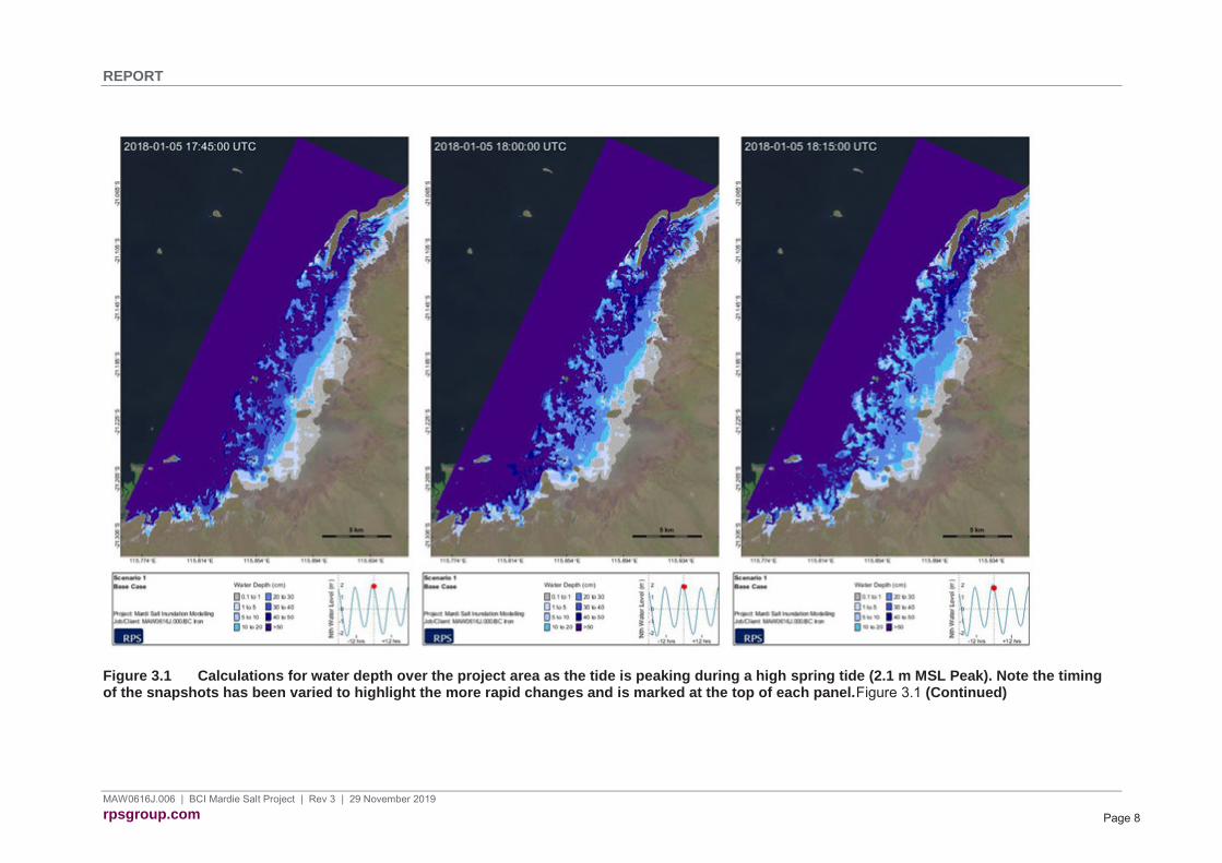
Simulation of tidal inundation over the existing landform (Base Case) indicates that water floods onto the land within the project area when tidal levels offshore are approaching high tide at tide levels of 1.2m MSL or higher.

Flooding onto the land occurs via multiple pathways:

• water floods onto the coastal margin through the mangrove zone and lower sections of the coast and floods onto the land surrounding the creeks.

• water floods out of the creeks from multiple low points that occur along the full length of the creeks and floods out onto the surrounding land via erosion channels.

• water floods from the terminal ends of the creeks and flows directly to the claypans beyond.

Water delivered from multiple pathways by high spring tides tends to merge over the land surrounding the creeks and then flood out to form a shallow lake over the clay pan area. The water floods out over the clay pan as a surge. The extent of the flooded area varies with the tidal level offshore, which generates the head of water to force the surge, and the time required for water to flood out over the surrounding land.

The landward extent of the flooded area is limited by the volume of water that floods into the area (dependent on the tide level) and higher ground on the hinterland side. There is a substantially wider area of low-lying clay pan available to capture water over the northern and central parts of the Mardie project area and only a narrow margin available at the southern end of the project area before high ground is met.

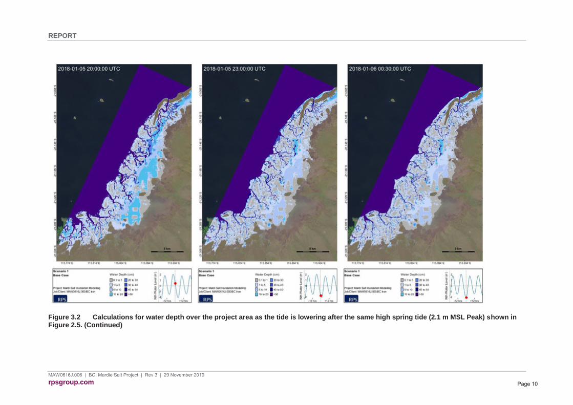
As the tide drops offshore, water levels in the creeks and at the coast lower below the land height and water begins to drain back via multiple drainage channels. The simulations indicate that most of the water drains back on a receding tide, although remnants of the water may be retained in localised dips in the topography.

The simulations demonstrate that flood surges commence just as the tide is peaking during higher tides and that, if sufficient water-volume is released onto the flood-plain, the flood waters surge out over the clay pan area over a period of the order of 40 - 45 minutes. Near the coast the drainage of water back towards the sea begins immediately after the tidal peak passes; hence, the flood surge is still occurring upstream after the peak in tide. The simulations also reveal that water drains back from the clay pan areas more slowly than the flood surge arrives, requiring 3 - 5 hours depending upon the water level. Drainage will be complete by the time that low tide is reached at the coast and, as a consequence, most of the flooding area does not appear to hold surface water over subsequent tides. Instead, these areas fill up and drain over subsequent tides of sufficient height.

Different wetting periods were observed in the simulation during different stages of the spring-neap cycle. During the highest spring-tides that were simulated, the claypan areas were overtopped by water for periods of 4 to 6 hours every 12 hours. Hence, the period over which the ground could dry was limited to less than 6 hours on each tidal cycle. In contrast, the simulations indicated increased time between wetting as the tidal levels decreased towards neap tides and that no flooding of the clay pan areas will occur when high tide levels fall below approximately 1.1-1.2 m MSL. These conditions occur over periods spanning 7-10 days. Consequently, the claypans will not be overtopped for 7-10 days over neap-tide periods. Hence, in addition to the fluctuations in water depth over the clay pans, fluctuations in tidal levels will have consequence for the retention of moisture in the soil within the algal mat areas. Review of the time-lapse imagery also indicates that salt precipitates over the ground surface when the ground does not wet after 2-3 days, with potential consequence for the osmotic pressure exerted on the algal mats and organisms that predate on the algae.

REPORT


Figure 3.1 Calculations for water depth over the project area as the tide is peaking during a high spring tide (2.1 m MSL Peak). Note the timing of the snapshots has been varied to highlight the more rapid changes and is marked at the top of each panel.

REPORT


Figure 3.1 Calculations for water depth over the project area as the tide is peaking during a high spring tide (2.1 m MSL Peak). Note the timing of the snapshots has been varied to highlight the more rapid changes and is marked at the top of each panel.Figure 3.1 (Continued)

REPORT


Figure 3.2 Calculations for water depth over the project area as the tide is lowering after the same high spring tide (2.1 m MSL Peak) shown in Figure 2.5.

REPORT


Figure 3.2 Calculations for water depth over the project area as the tide is lowering after the same high spring tide (2.1 m MSL Peak) shown in Figure 2.5. (Continued)

REPORT


3.2 Effect of the pond walls on inundation

Simulation of tidal inundation over the Mardie project area with the pond walls in place (Pond Case) indicates an effect of the walls on the landward movement of water at the northern and southern parts commences at tidal peaks exceeding around 1.2 m, because the pond walls would extend up to the terminal points of the creeks in these areas (Figure 3.3). The effect is expressed as a block of the water that would normally flow inland onto the low-lying land beyond the walls. Due to the multiple flow paths for water, there are no apparent effects of the wall on the wetting of land on the seaward side of the walls. None of the areas on the seaward side of the walls that flooded in the Base Case remained dry in the Pond Case.

The movement of water over the central part of the project where the pond walls are further inland remains similar to the Base Case at tide levels lower than ~ 1.8 m MSL because water can freely flood in and drain out along the same pathways and the flooding level does not reach the pond walls. During more extreme spring-tides; however, water is calculated to flood out to reach the pond walls which act to block the progress of water onto portions of the land beyond. The floodwaters reach the walls closer to the north and south at lower tides and the central walls at higher tides (Figure 3.4).

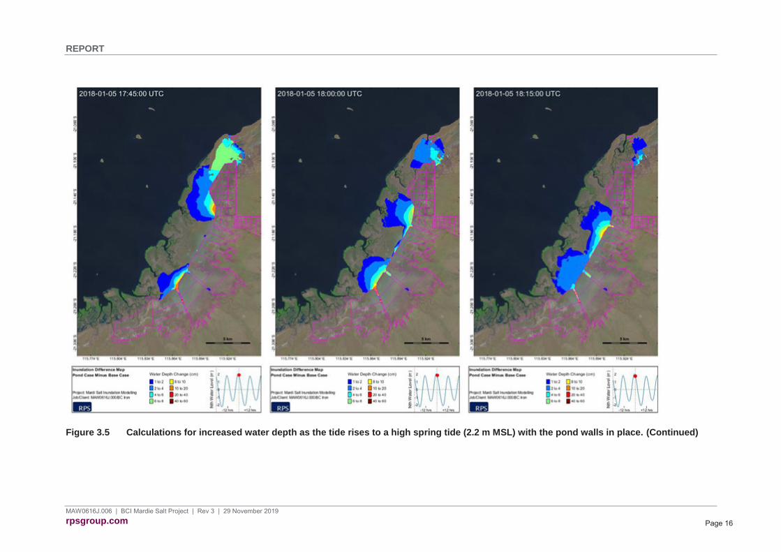
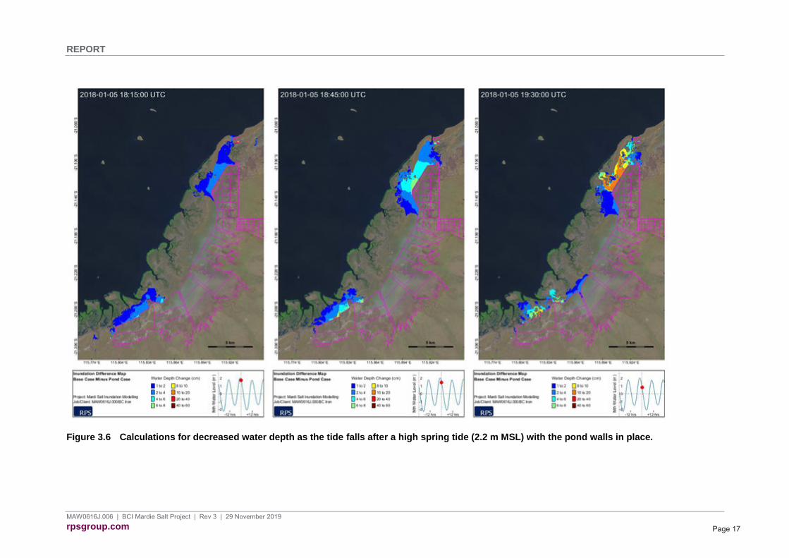
The effect of the pond walls was further investigated by calculating differences in water depth at each time-step in the simulations for the Base Case and the Pond Case, under the influence of the same sequence of tidal elevations (Figure 3.5 and Figure 3.6). The barrier effect of the walls is shown to cause a relatively small increase in the depth of water calculated for the clay pan area during the flooding phase only at the higher tides during the spring tide phase. Largest increases in depth are revealed for areas within a few hundred metres of the walls at the far northern and southern sections. These differences are short-lived, persisting for 15 - 30 minutes at most, as the increased water depth is shed to surrounding areas. The shedding of water is revealed as the propagation of water over the clay pans in the centre of the project area.

Another effect of the pond walls demonstrated by the simulation is that the water held up by the walls would drain away faster than in the Base Case because water would otherwise drain back over the land beyond the walls – a slower process than drainage from a freestanding body of water. The largest effect on the drainage of water is indicated for the same areas where the pond walls are expected to cause the largest, short-lived, rise in the water depth. This pattern suggests a slight shift in the timing of inundation over a full tidal cycle, with the largest effect expressed at the sections of wall at the far north and south, where the pond walls extend further forward.

The magnitude of the shift was investigated further by calculating a time-series of water depth for three locations immediately in front of the walls: locations at the far north and far south where the largest changes to the flooding and draining depth where illustrated and at a central location (Figure 3.7). The plot was generated for the highest tide during the sample period (~2.2 m MSL). Hence, for an extreme, annual, event. These plots confirm that the phase and magnitude of water depth remains similar and that differences are of the order of 10-20 cm water depth.

REPORT


Figure 3.3 Calculations for water depth over the project area as the tide is rising to a spring tide (1.8 m MSL) for the Pond Case.

REPORT


Figure 3.4 Calculations for water depth over the project area as the tide is rising to a high spring tide (2.2 m MSL) for the Pond Case. Times correspond to images in Figure 3.1

REPORT


Figure 3.4 Calculations for water depth over the project area as the tide is rising to a high spring tide (2.2 m MSL) for the Pond Case. Times correspond to images in Figure 3.1 (Continued)

REPORT


Figure 3.5 Calculations for increased water depth as the tide rises to a high spring tide (2.2 m MSL) with the pond walls in place.

REPORT


Figure 3.5 Calculations for increased water depth as the tide rises to a high spring tide (2.2 m MSL) with the pond walls in place. (Continued)

REPORT


Figure 3.6 Calculations for decreased water depth as the tide falls after a high spring tide (2.2 m MSL) with the pond walls in place.

REPORT


Figure 3.6 Calculations for decreased water depth as the tide falls after a high spring tide (2.2 m MSL) with the pond walls in place. (Continued)

REPORT


Figure 3.7 Comparison of the frequency of different water depths between the Pond Case and Base Case at locations near the walls. The Y-axis shows water depth in cm. The X-axis shows the percentile exceedance (e.g. the 90th percentile would be exceeded 10% of the time; the 60th percentile would be exceeded 40% of the time). Line colours correspond to X marks on the map. Lines with crosses represent the Pond Case.

REPORT


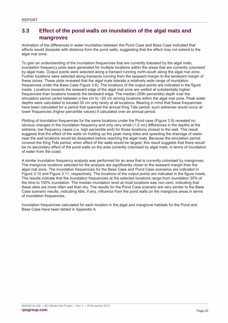
3.3 Effect of the pond walls on inundation of the algal mats and

mangroves

Animation of the differences in water inundation between the Pond Case and Base Case indicated that effects would dissipate with distance from the pond walls, suggesting that the effect may not extend to the algal mat zone.

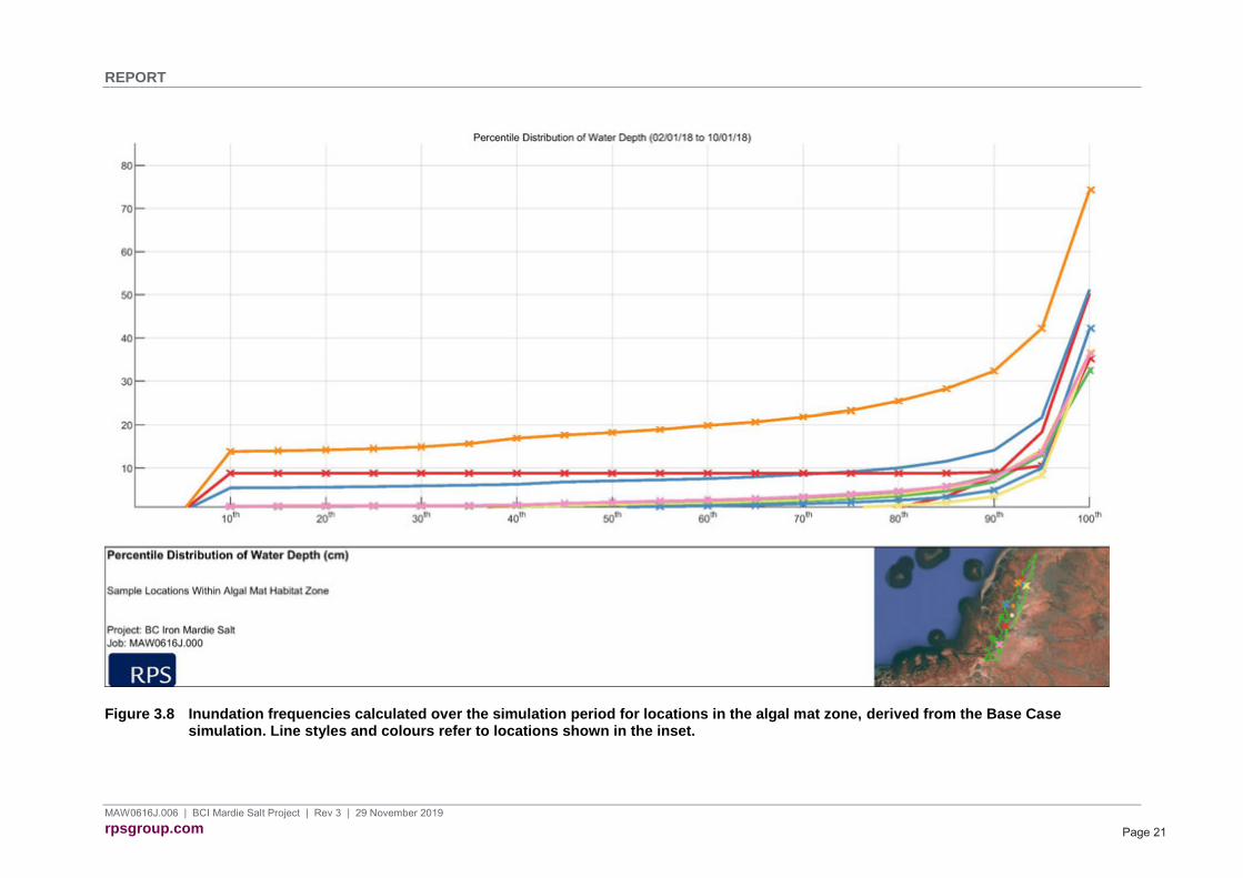
To gain an understanding of the inundation frequencies that are currently tolerated by the algal mats, inundation frequency plots were generated for multiple locations within the areas that are currently colonised by algal mats. Output points were selected along a transect running north-south along the algal mat zone. Further locations were selected along transects running from the seaward margin to the landward margin of these zones. These plots revealed that the algal mats tolerate a relatively wide range of inundation frequencies under the Base Case Figure 3.8). The locations of the output points are indicated in the figure insets. Locations towards the seaward edge of the algal mat zone are wetted at substantially higher frequencies than locations towards the landward edge. The median (50th percentile) depth over the simulation period varied between a few cm to ~20 cm among locations within the algal mat zone. Peak water depths were calculated to exceed 30 cm only rarely at all locations. Bearing in mind that these frequencies have been calculated for a period that spanned the annual King Tide period, such extremes would occur at lower frequencies (higher percentile values) if calculated over an annual period.

Plotting of inundation frequencies for the same locations under the Pond case (Figure 3.9) revealed no obvious changes in the inundation frequency and only very small (1-2 cm) differences in the depths at the extreme, low frequency cases (i.e. high percentile end) for those locations closest to the wall. This result suggests that the effect of the walls on holding up the peak rising tides and speeding the drainage of water near the wall locations would be dissipated before reaching the algal mats. Because the simulation period covered the King Tide period, when effect of the walls would be largest, this result suggests that there would be no secondary effect of the pond walls on the area currently colonised by algal mats, in terms of inundation of water from the coast.

A similar inundation frequency analysis was performed for an area that is currently colonised by mangroves. The mangrove locations selected for the analysis are significantly closer to the seaward margin than the algal mat zone. The inundation frequencies for the Base Case and Pond Case scenarios are indicated in Figure 3.10 and Figure 3.11, respectively. The locations of the output points are indicated in the figure insets. The results indicate that the inundation frequencies at the selected locations range from inundation 35% of the time to 100% inundation. The median inundation level at most locations was non-zero, indicating that these sites are more often wet than dry. The results for the Pond Case scenario are very similar to the Base Case scenario results, indicating little, if any, influence from the pond walls on the mangrove areas in terms of inundation frequencies.

Inundation frequencies calculated for each location in the algal and mangrove habitats for the Pond and Base Case have been tabled in Appendix A.

REPORT


Figure 3.8 Inundation frequencies calculated over the simulation period for locations in the algal mat zone, derived from the Base Case simulation. Line styles and colours refer to locations shown in the inset.

REPORT


Figure 3.9 Inundation frequencies calculated over the simulation period for locations in the algal mat zone, derived from the Pond Case simulation. Line styles and colours refer to locations shown in the inset.

REPORT


Figure 3.10 Inundation frequencies calculated over the simulation period for locations in the mangrove zone, derived from the Base Case simulation. Line styles and colours refer to locations shown in the inset.

REPORT


Figure 3.11 Inundation frequencies calculated over the simulation period for locations in the mangrove zone, derived from the Pond Case simulation. Line styles and colours refer to locations shown in the inset.

REPORT


3.4 Effect of the pond walls on inundation with sea level rise

Simulations of coastal inundation imposing an additional 0.9 m of sea level rise (following EPA recommendations for allowance over 100 years for coastal hazard assessment) indicates that the project area would still wet and dry, exposing the existing mangrove area at lower tides but inundation of the clay pans would occur more frequently. For example, the current high tide that is reached annually during a King Tide (2.2 m MSL in January 2018) would occur at the frequency of the current lower limit for inundation of the clay pans (1.2 m MSL), a level that occurs > 15 days per month over the Spring tidal phase. This outcome suggests that the clay pan area would remain wet at a higher frequency of the time, with a reduced time between flooding events over a reduced neap, dry, period.

Conversely, water flooding onto the land under the same astronomical tides would flood further inland during more high tide events. There is a natural limit to the distance that water would flood inland that is imposed by the higher ground of the hinterland. Higher ground occurs closer to the coastline over the northern part of the project area and extends further away further south. Consequently, the simulations show that water would flood out further inland over the more southern portion of the project area at a given tidal level compared to the contemporary Base Case (Figure 3.12). This result suggests that there would be an inland extension to the areas that would be inundated at the rate that currently occurs over the algal mats. The limits to water spread imposed by higher ground would also force greater water depth over the area that currently supports algal mats during spring tides.

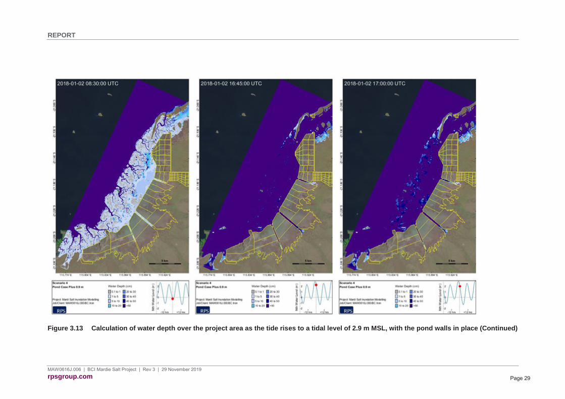
If the pond walls were in place, they would block the inland flow of water over areas that would otherwise be flooded, resulting in higher water depths over the seaward land area during spring tides. Simulations indicate that there would remain an area of clay pan that wets and dries and that the whole of the Mardie Project area would fill to a depth > 0.5 m during the annual King Tide (Figure 3.13).

The inundation frequency analysis (Section 3.3) was repeated for the sea level rise scenario. The effect of sea level rise on the inundation frequency for the algal mat zone was calculated for the Base Case (Figure 3.15) and the Pond Case (Figure 3.16). Similarly, the effect of sea level rise on the inundation frequency for the mangrove zone was calculated for the Base Case (Figure 3.16) and the Pond Case (Figure 3.17).

REPORT


Figure 3.12 Calculation of water depth over the project area as the tide rises to a tidal level of 2.9 m MSL

REPORT


Figure 3.12 Calculation of water depth over the project area as the tide rises to a tidal level of 2.9 m MSL (Continued)

REPORT


Figure 3.13 Calculation of water depth over the project area as the tide rises to a tidal level of 2.9 m MSL, with the pond walls in place

REPORT


Figure 3.13 Calculation of water depth over the project area as the tide rises to a tidal level of 2.9 m MSL, with the pond walls in place (Continued)

REPORT


Figure 3.14 Inundation frequencies calculated over the simulation period for locations in the algal mat zone, derived from the Base Case simulation with an additional 0.9 m of sea level rise. Line styles and colours refer to locations shown in the inset.

REPORT


Figure 3.15 Inundation frequencies calculated over the simulation period for locations in the algal mat zone, derived from the Pond Case simulation with an additional 0.9 m of sea level rise. Line styles and colours refer to locations shown in the inset.

REPORT


Figure 3.16 Inundation frequencies calculated over the simulation period for locations in the mangrove zone, derived from the Base Case simulation with an additional 0.9 m of sea level rise. Line styles and colours refer to locations shown in the inset.

REPORT


Figure 3.17 Inundation frequencies calculated over the simulation period for locations in the mangrove zone, derived from the Pond Case simulation with an additional 0.9 m of sea level rise. Line styles and colours refer to locations shown in the inset

REPORT


4 APPENDIX

4.1 Inundation frequency data

REPORT


Table 4-1 Base case in algal mats

Zone Algal Mat

Case Base

Sample Location Percentile Distribution of Water Depth (cm)

Longitude Latitude 0 5 10 15 20 25 30 35 40 45 50 55 60 65 70 75 80 85 90 95 100

115.903 -21.1451 0 0 0.9 0.9 0.9 0.9 0.9 0.9 0.9 0.9 0.9 0.9 0.9 0.9 0.9 0.9 0.9 3.4 7.9 18.3 50.3

115.8977 -21.1518 0 0 13.8 14 14.2 14.5 14.9 15.6 16.9 17.6 18.2 18.9 19.9 20.6 21.8 23.2 25.4 28.2 32.3 42.2 74.3

115.9038 -21.1537 0 0 5.4 5.5 5.6 5.7 5.9 6 6.2 6.8 7 7.3 7.5 8 8.5 9.1 10 11.6 14.1 21.7 51.2

115.9092 -21.1553 0 0 0.7 0.7 0.7 0.7 0.7 0.7 0.7 0.7 0.7 0.7 0.7 0.7 0.7 0.9 1.3 2 3.4 8.3 36.7

115.8993 -21.1718 0 0 0.7 0.7 0.7 0.7 0.7 0.7 1 1.3 1.4 1.6 1.8 2.1 2.4 2.9 3.5 4.6 6.8 13.1 36.2

115.8805 -21.1822 0 0 0.6 0.6 0.6 0.6 0.6 0.7 0.7 0.9 1 1.1 1.2 1.4 1.7 2 2.5 3.2 4.9 10 42.2

115.8905 -21.1842 0 0 0.8 0.8 0.8 0.8 0.8 0.9 1.2 1.5 1.7 1.9 2.2 2.5 2.9 3.4 4.1 5.3 7.9 14 36.4

115.8994 -21.185 0 0 1 1.1 1.1 1.2 1.2 1.2 1.3 1.8 2 2.3 2.5 2.8 3.2 3.8 4.5 5.8 8.2 13 32.5

115.889 -21.1978 0 0 0.6 0.6 0.6 0.6 0.6 0.7 1 1.4 1.6 1.8 2 2.3 2.7 3.3 4 5.4 8 13.8 34.8

115.8787 -21.2126 0 0 8.8 8.8 8.8 8.8 8.8 8.8 8.8 8.8 8.8 8.8 8.8 8.8 8.8 8.8 8.8 8.8 9 10.5 35.2

115.8707 -21.2389 0 0 1.2 1.3 1.3 1.3 1.3 1.3 1.4 1.8 2.1 2.3 2.6 2.9 3.4 4 4.7 5.7 7.8 13.6 36.3

REPORT


Table 4-2 Pond case in algal mats

Zone Algal Mat

Case Pond



115.903 -21.1451 0 0 0.8 0.8 0.8 0.8 0.8 0.8 0.8 0.8 0.8 0.8 0.8 0.8 0.8 0.8 1.8 4 7.5 15.8 56.3

115.8977 -21.1518 0 0 13.8 13.9 14.2 14.5 14.9 15.6 16.8 17.5 18.2 18.8 19.5 20.2 21.2 22.7 24.7 27.6 31.5 39.9 79.4

115.9038 -21.1537 0 0 5.7 5.7 5.7 5.7 5.7 5.7 6 6.3 6.4 6.6 6.9 7.2 7.5 8 8.6 9.9 12.9 19.2 59.4

115.9092 -21.1553 0 0 0.7 0.7 0.7 0.7 0.7 0.7 0.7 0.7 0.7 0.7 0.7 0.7 0.7 0.7 0.7 0.8 1.7 5.8 45.5

115.8993 -21.1718 0 0 0.6 0.6 0.6 0.6 0.6 0.7 0.9 1 1.2 1.3 1.5 1.7 1.9 2.2 2.8 3.7 5.6 12.3 43.9

115.8805 -21.1822 0 0 0.6 0.6 0.6 0.6 0.6 0.6 0.7 0.8 0.8 0.9 1 1.2 1.4 1.7 2.1 2.8 4.4 10.6 42.6

115.8905 -21.1842 0 0 0.7 0.7 0.7 0.7 0.7 0.8 1 1.2 1.4 1.5 1.7 2 2.3 2.6 3.2 4.2 6.4 13.4 43.7

115.8994 -21.185 0 0 0.7 0.7 0.7 0.7 0.7 0.8 1 1.3 1.4 1.6 1.7 1.9 2.2 2.6 3.1 4.1 6.1 11.7 46.2

115.889 -21.1978 0 0 0.5 0.5 0.5 0.5 0.5 0.6 0.9 1.1 1.3 1.5 1.7 1.9 2.1 2.5 3.1 4.2 6.4 12.4 43.2

115.8787 -21.2126 0 0 8.8 8.8 8.8 8.8 8.8 8.8 8.8 8.8 8.8 8.8 8.8 8.8 8.8 8.8 8.8 8.8 9 10.7 41.3

115.8707 -21.2389 0 0 0.6 0.6 0.6 0.6 0.6 0.6 0.7 0.8 0.9 1 1.2 1.4 1.5 1.7 2 2.6 3.9 9.7 48.1

REPORT


Table 4-3 Comparison of percentile distribution of water depth (Pond Case - Base Case) in algal mats

Zone Algal Mat

Case Pond Case minus Base Case



115.903 -21.1451 0 0 0 0 0 0 0 0 0 0 0 0 0 0 0 0 0.9 0.6 -0.4 -2.5 5.9

115.8977 -21.1518 0 0 0 0 0 0 0 0 -0.1 -0.1 -0.1 -0.1 -0.4 -0.5 -0.6 -0.5 -0.7 -0.6 -0.8 -2.2 5.1

115.9038 -21.1537 0 0 0.3 0.2 0.1 0 -0.2 -0.3 -0.2 -0.5 -0.6 -0.7 -0.7 -0.8 -1 -1.2 -1.4 -1.6 -1.3 -2.5 8.1

115.9092 -21.1553 0 0 0 0 0 0 0 0 0 0 0 0 0 0 0 -0.2 -0.6 -1.2 -1.7 -2.5 8.8

115.8993 -21.1718 0 0 -0.1 -0.1 -0.1 -0.1 -0.1 -0.1 -0.1 -0.2 -0.3 -0.3 -0.4 -0.4 -0.5 -0.6 -0.7 -0.9 -1.2 -0.7 7.8

115.8805 -21.1822 0 0 0 0 0 0 0 0 0 -0.1 -0.1 -0.2 -0.2 -0.2 -0.3 -0.3 -0.5 -0.5 -0.5 0.6 0.4

115.8905 -21.1842 0 0 -0.1 -0.1 -0.1 -0.1 -0.1 -0.1 -0.1 -0.3 -0.3 -0.4 -0.4 -0.5 -0.6 -0.8 -0.9 -1.2 -1.4 -0.6 7.3

115.8994 -21.185 0 0 -0.3 -0.4 -0.4 -0.5 -0.5 -0.4 -0.3 -0.6 -0.6 -0.7 -0.8 -0.8 -1 -1.2 -1.4 -1.6 -2 -1.3 13.7

115.889 -21.1978 0 0 -0.1 -0.1 -0.1 -0.1 -0.1 -0.1 -0.1 -0.2 -0.3 -0.4 -0.4 -0.4 -0.6 -0.8 -0.9 -1.2 -1.7 -1.3 8.5

115.8787 -21.2126 0 0 0 0 0 0 0 0 0 0 0 0 0 0 0 0 0 0 0 0.1 6.2

115.8707 -21.2389 0 0 -0.6 -0.7 -0.7 -0.7 -0.7 -0.7 -0.8 -1 -1.2 -1.3 -1.4 -1.6 -1.9 -2.2 -2.6 -3.1 -4 -3.9 11.7

REPORT


Table 4-4 Base case with 0.9 m sea level rise in algal mats

Zone Algal Mat

Case Base Case Plus 90cm



115.903 -21.1451 0 0.9 0.9 0.9 0.9 1.9 3.2 4.9 6.5 8.6 10.5 13.1 16.7 21.5 29.0 37.7 49.0 62.8 80.8 101.5 144.5

115.8977 -21.1518 0 21.2 23.7 24.8 25.8 26.9 28.1 29.7 31.2 33.2 35.3 37.7 41.2 45.8 53.8 61.7 73.3 87.9 105.2 126.1 168.5

115.9038 -21.1537 0 9.0 10.4 11.2 11.7 12.3 13 13.8 14.6 15.7 17.0 19.0 21.8 26.7 32.6 40.6 52.4 66.1 83.2 105.3 147.4

115.9092 -21.1553 0 1.1 1.8 2.2 2.4 2.7 3.0 3.5 4.1 4.9 6.1 7.6 10.1 13.7 18.8 25.9 36.8 49.9 66.6 89.8 134.0

115.8993 -21.1718 0 3.1 4.4 5.2 5.7 6.3 7.1 7.9 9.0 10.3 11.9 14.1 17.1 20.6 24.8 31.7 42.3 53.0 68.5 90.8 137.0

115.8805 -21.1822 0 2.1 3.0 3.5 3.9 4.3 4.7 5.3 6.0 6.9 8.0 9.5 1.02 16 22.2 29.3 41.1 55.2 73.1 93.3 134.5

115.8905 -21.1842 0 3.7 5.3 6.4 7.0 7.8 8.5 9.4 10.5 11.9 13.6 15.8 18.6 22.3 26.6 33.9 43.9 54.3 69.8 90.1 136.2

115.8994 -21.185 0 4.1 5.9 6.9 7.6 8.2 9.1 10.1 11.2 12.7 14.4 16.5 19.3 22.7 27.5 34.3 42.8 53.4 69.7 90.1 138.2

115.889 -21.1978 0 3.6 5.7 7.1 8 8.7 9.6 10.5 11.7 13.1 14.9 17.0 19.9 23.5 28.2 35.0 43.5 53.9 69.8 90.3 135.4

115.8787 -21.2126 0 8.8 8.8 8.8 8.9 8.9 9.0 9.2 9.5 9.9 10.9 13.1 16.4 2.00 25.1 32.2 41.1 50.4 68.1 86.9 128.0

115.8707 -21.2389 0 4.4 6.7 8.5 10.2 11.5 12.6 14 15.5 17.3 19.6 22.2 25.5 29.6 34.6 40.9 48.1 58.9 71.2 88.3 126.0

REPORT


Table 4-5 Pond case with 0.9 m sea level rise in algal mats

Zone Algal Mat

Case Pond Case Plus 90cm



115.903 -21.1451 0 0.8 0.8 0.8 0.8 0.8 1.5 2.4 3.4 5 6.6 8.9 11.2 14.9 20.7 29.9 42.6 60.9 81.2 106.9 157.6

115.8977 -21.1518 0 20.2 21.1 21.7 22.5 23.3 24.3 25.5 27 28.6 30.5 32.8 35.2 39 44.8 53.7 66.4 84.4 105 131.1 181

115.9038 -21.1537 0 7.6 8 8.2 8.5 8.9 9.3 9.9 10.6 11.5 12.6 13.9 15.8 18.9 24.2 32.6 43.4 63.5 84.2 111.3 160.4

115.9092 -21.1553 0 0.7 0.7 0.7 0.7 0.8 0.8 1 1.3 1.5 2 2.7 3.9 5.8 9.9 16.7 28.3 48.2 68.9 96.6 146.1

115.8993 -21.1718 0 2.3 2.7 2.9 3.2 3.5 3.8 4.3 4.8 5.5 6.3 7.5 9.3 12 15.8 22 31.8 49.1 69.2 99 148.6

115.8805 -21.1822 0 1.6 1.8 2 2.2 2.4 2.6 2.9 3.3 3.7 4.4 5.3 6.7 9 14.4 23.2 34.1 52 71.2 95.9 146

115.8905 -21.1842 0 2.7 3.2 3.4 3.7 4 4.4 4.9 5.5 6.2 7.2 8.5 10.2 12.9 16.8 22.3 32.6 47.5 66.4 98.5 147.4

115.8994 -21.185 0 2.7 3.2 3.5 3.7 4.1 4.5 4.9 5.5 6.2 7.1 8.2 9.9 12.1 15.3 20.3 28.9 45.5 66.7 98.7 148

115.889 -21.1978 0 2.6 3.1 3.4 3.7 4 4.4 4.9 5.5 6.2 7.2 8.4 10.1 12.6 16.3 22.1 31 45.4 66.2 97.5 148.9

115.8787 -21.2126 0 8.8 8.8 8.8 8.8 8.8 8.9 8.9 8.9 9 9.1 9.4 9.8 10.7 13.6 19.1 28.9 43.7 63.7 93.3 144

115.8707 -21.2389 0 1.5 2.2 2.6 2.8 3 3.3 3.6 4 4.4 5 5.9 7.2 9.8 14.1 21.3 32.3 51.1 71.9 100.2 150

REPORT


Table 4-6 Comparison of percentile distribution of water depth (Pond Case - Base Case) in algal mats with 0.9 m sea level rise

Zone Algal Mat

Case Pond Case Plus 90cm minus Base Case Plus 90cm



115.903 -21.1451 0 0 0 0 -0.1 -1 -1.7 -2.5 -3.1 -3.6 -3.9 -4.2 -5.4 -6.6 -8.3 -7.8 -6.4 -1.8 0.4 5.4 13.1

115.8977 -21.1518 0 -0.9 -2.5 -3.1 -3.3 -3.6 -3.8 -4.2 -4.2 -4.7 -4.8 -4.9 -6 -6.8 -8.9 -8 -6.9 -3.6 -0.2 5 12.5

115.9038 -21.1537 0 -1.4 -2.5 -2.9 -3.2 -3.5 -3.7 -3.9 -4 -4.2 -4.4 -5 -6 -7.8 -8.4 -8 -8.9 -2.6 1 5.9 12.9

115.9092 -21.1553 0 -0.4 -1.1 -1.5 -1.7 -1.9 -2.2 -2.5 -2.8 -3.3 -4.1 -4.9 -6.2 -7.9 -8.9 -9.2 -8.5 -1.7 2.3 6.8 12.1

115.8993 -21.1718 0 -0.7 -1.7 -2.3 -2.5 -2.9 -3.3 -3.6 -4.2 -4.8 -5.5 -6.6 -7.8 -8.6 -9 -9.6 -10.5 -4 0.7 8.2 11.6

115.8805 -21.1822 0 -0.5 -1.1 -1.5 -1.7 -1.9 -2.1 -2.4 -2.7 -3.1 -3.5 -4.2 -5.3 -7 -7.8 -6.1 -7 -3.2 -1.8 2.6 11.4

115.8905 -21.1842 0 -1 -2.2 -3 -3.3 -3.7 -4.1 -4.5 -5 -5.7 -6.4 -7.3 -8.4 -9.4 -9.8 -11.6 -11.3 -6.8 -3.4 8.4 11.2

115.8994 -21.185 0 -1.4 -2.7 -3.4 -3.8 -4.2 -4.6 -5.1 -5.7 -6.5 -7.3 -8.3 -9.4 -10.6 -12.1 -14 -13.9 -7.9 -3 8.6 9.8

115.889 -21.1978 0 -1 -2.6 -3.7 -4.3 -4.7 -5.2 -5.6 -6.3 -6.9 -7.8 -8.6 -9.8 -10.9 -11.9 -12.9 -12.5 -8.5 -3.6 7.2 13.5

115.8787 -21.2126 0 0 0 0 -0.1 -0.1 -0.2 -0.3 -0.5 -0.9 -1.8 -3.8 -6.6 -9.3 -11.4 -13.1 -12.2 -6.7 -4.4 6.4 16

115.8707 -21.2389 0 -2.9 -4.5 -5.8 -7.4 -8.5 -9.3 -10.4 -11.5 -12.9 -14.6 -16.3 -18.2 -19.8 -20.5 -19.7 -15.8 -7.8 0.7 11.9 24

REPORT


Table 4-7 Base case in mangroves

Zone Mangrove

Case Base Case



115.9248 -21.0876 0 7.3 7.3 7.4 7.4 7.5 7.5 7.5 7.6 7.6 7.6 7.6 7.6 7.7 7.7 23.5 41.5 60.8 79.1 95.7 125.7

115.9112 -21.1130 0 66.7 66.8 66.8 66.8 66.8 66.8 66.9 67 77.2 97.6 122.7 147.7 169.6 193.7 215.3 235.6 251 262.9 277.2 311.5

115.8997 -21.1203 0 1.9 1.9 1.9 2 2 2 2.1 2.1 2.1 2.1 2.1 2.2 2.2 11 28.5 43.2 63.7 81.9 100.3 136.7

115.8554 -21.1933 0 2.5 2.6 2.7 2.7 2.7 2.7 2.7 2.7 2.7 2.8 2.8 2.8 19.7 38.5 55.9 74.5 94.5 116.6 137 176.4

115.8665 -21.2212 0 4.4 4.4 4.5 4.8 4.9 7 17.9 27.2 37.8 51.5 69.4 86.3 107.7 129 148.4 170.3 190 206.2 217.8 251.2

115.8209 -21.2508 0 7.3 7.3 7.4 7.4 7.4 7.4 7.5 7.5 7.6 15.4 36.8 57.9 81.3 101.9 120.6 138 158.6 178.6 197.9 240.1

115.7946 -21.2617 0 1.5 1.5 1.5 1.5 1.5 1.6 1.6 1.6 1.6 1.7 10.2 31.2 53.6 74.7 92.3 110.6 131.6 151.2 172.7 213.4

115.8212 -21.2683 14.9 101.7 102.5 104.3 105.5 107 108.4 109.4 111.3 113.3 115.6 130.4 152.8 172.8 198.8 217.3 233.7 254.5 275.4 296.5 336.4

115.7955 -21.2756 0 14.1 14.2 14.2 14.2 14.3 14.3 14.3 18.2 36.7 58.3 78.4 102.8 126.7 147.3 166.9 181.7 203.3 223 246.6 286.7

115.8204 -21.2786 0 0 16.9 16.9 16.9 16.9 16.9 17 17.2 17.4 17.6 17.8 18.2 18.6 19.2 20.2 22 25.8 33.1 49.3 93.1

REPORT


Table 4-8 Pond case in mangroves

Zone Mangrove

Case Pond Case



115.9248 -21.0876 0 7.3 7.3 7.4 7.4 7.5 7.5 7.5 7.5 7.6 7.6 7.6 7.6 7.6 7.7 23.5 41.1 60.7 78.1 95.9 132.1

115.9112 -21.1130 0 66.7 66.8 66.8 66.8 66.8 66.8 66.8 66.8 75.2 93.5 118.8 140.4 166.5 189.2 210.2 231 246.9 262.2 278.7 316.5

115.8997 -21.1203 0 1.9 1.9 2 2 2 2 2 2.1 2.2 2.2 2.2 2.2 2.2 3.8 22.9 39.6 62.9 81.3 100.4 141.4

115.8554 -21.1933 0 2.5 2.6 2.6 2.7 2.7 2.7 2.7 2.8 2.8 2.8 2.8 2.8 19.7 38.5 55.9 74.5 94.4 116.5 137.1 176.3

115.8665 -21.2212 0 4.4 4.4 4.4 4.8 4.9 5 5.1 15.8 28.1 43.7 62.7 80.7 103 124.4 146.1 168.1 188 204.9 218.9 254.8

115.8209 -21.2508 0 7.3 7.3 7.3 7.4 7.4 7.4 7.5 7.5 7.6 15.4 36.8 57.9 81.3 101.9 120.7 138 158.7 178.5 198 239.6

115.7946 -21.2617 0 1.4 1.5 1.5 1.5 1.6 1.6 1.6 1.6 1.6 1.7 10.2 31.3 53.5 74.7 92.3 110.6 131.6 151.1 172.2 212.4

115.8212 -21.2683 14.9 101.7 102.2 103.3 104.2 104.8 105.1 106.1 106.2 106.9 110.3 127 150.2 172.6 198 214.5 233.1 252.4 273.2 294.8 334.6

115.7955 -21.2756 0 14.1 14.2 14.2 14.2 14.2 14.2 14.3 18.2 36.7 58.3 78.3 102.3 126.6 147.1 166.7 181.7 203 222.7 246.4 285

115.8204 -21.2786 0 0 0 0 0 0 0 0 0 0 0 0 0 0 0 0 0 0 0 0 0

REPORT


Table 4-9 Comparison of percentile distribution of water depth (Pond Case - Base Case) in mangroves

Zone Mangrove

Case Pond Case Minus Base Case



115.9248 -21.0876 0 0 0 0 0 0 0 0 0 0 0 0 0 0 0 0 0.9 0.6 -0.4 -2.5 5.9

115.9112 -21.1130 0 0 0 0 0 0 0 0 -0.1 -0.1 -0.1 -0.1 -0.4 -0.5 -0.6 -0.5 -0.7 -0.6 -0.8 -2.2 5.1

115.8997 -21.1203 0 0 0.3 0.2 0.1 0 -0.2 -0.3 -0.2 -0.5 -0.6 -0.7 -0.7 -0.8 -1 -1.2 -1.4 -1.6 -1.3 -2.5 8.1

115.8554 -21.1933 0 0 0 0 0 0 0 0 0 0 0 0 0 0 0 -0.2 -0.6 -1.2 -1.7 -2.5 8.8

115.8665 -21.2212 0 0 -0.1 -0.1 -0.1 -0.1 -0.1 -0.1 -0.1 -0.2 -0.3 -0.3 -0.4 -0.4 -0.5 -0.6 -0.7 -0.9 -1.2 -0.7 7.8

115.8209 -21.2508 0 0 0 0 0 0 0 0 0 -0.1 -0.1 -0.2 -0.2 -0.2 -0.3 -0.3 -0.5 -0.5 -0.5 0.6 0.4

115.7946 -21.2617 0 0 -0.1 -0.1 -0.1 -0.1 -0.1 -0.1 -0.1 -0.3 -0.3 -0.4 -0.4 -0.5 -0.6 -0.8 -0.9 -1.2 -1.4 -0.6 7.3

115.8212 -21.2683 0 0 -0.3 -0.4 -0.4 -0.5 -0.5 -0.4 -0.3 -0.6 -0.6 -0.7 -0.8 -0.8 -1 -1.2 -1.4 -1.6 -2 -1.3 13.7

115.7955 -21.2756 0 0 -0.1 -0.1 -0.1 -0.1 -0.1 -0.1 -0.1 -0.2 -0.3 -0.4 -0.4 -0.4 -0.6 -0.8 -0.9 -1.2 -1.7 -1.3 8.5

115.8204 -21.2786 0 0 0 0 0 0 0 0 0 0 0 0 0 0 0 0 0 0 0 0.1 6.2

REPORT


Table 4-10 Base case with 0.9 m sea level rise in mangroves

Zone Mangrove

Case Base Case Plus 90cm



115.9248 -21.0876 0 5 10 15 20 25 30 35 40 45 50 55 60 65 70 75 80 85 90 95 100

115.9112 -21.1130 0 7.4 7.5 7.5 7.5 7.5 7.5 7.6 7.6 16.7 36.2 53.8 72.8 86.4 102.7 114.7 127 138.9 154.1 171.5 213.3

115.8997 -21.1203 66.7 69.8 79.7 92.5 109.5 127.2 149.3 175.6 202.3 226.7 246.5 258.5 267.9 277.7 288.2 297.6 310.6 323.9 340.8 358.5 398.1

115.8554 -21.1933 0 2.1 2.1 2.1 2.2 2.2 2.2 2.3 12.7 31.7 49.9 67.7 82.1 95.2 108.7 120.8 136.4 149.4 168 187.6 228.1

115.8665 -21.2212 0 2.5 2.6 2.6 2.6 2.7 2.8 2.8 9.8 28.7 44.6 63.6 84 108.1 127.3 146.6 164.2 184.4 205.8 226 266

115.8209 -21.2508 27.1 80.4 107.4 124.9 136.4 152.1 170 188.4 199 207 214.2 219.5 224.6 230.3 236.4 244.2 253.8 265.7 282 301.3 340.7

115.7946 -21.2617 7.1 7.3 7.5 7.6 7.6 15.3 33.2 47.6 65.5 84.7 104.8 126.5 147.1 170.8 190.8 210.1 228.4 249.9 269.9 290 329.6

115.8212 -21.2683 0 1.4 1.4 1.5 1.5 1.6 8.9 23.1 39.9 58.5 79.5 100.6 123.4 143.9 165.5 187.1 204.5 224.4 243.6 265.3 303.8

115.7955 -21.2756 95.9 103.2 106.3 110.2 113.2 115.8 128.6 145.6 165.6 188.2 209.6 229.5 250.5 269.5 286.3 306.9 325.2 346.4 364.4 385.8 424.9

115.8204 -21.2786 14 14.2 16 33.9 48.8 63.3 80 95 112.7 134.4 154.6 172.4 192 216.2 235.4 259.8 277.6 297.8 315.9 338.1 377.1

REPORT


Table 4-11 Pond case with 0.9 m sea level rise in mangroves

Zone Mangrove

Case Pond Case Plus 90cm



115.9248 -21.0876 0 7.4 7.5 7.5 7.6 7.6 7.6 7.6 7.6 8 28.6 49.5 68.9 82.8 99.2 114.1 126.9 140.1 157.3 175.5 212.5

115.9112 -21.1130 66.6 66.7 73.9 87.8 100.2 114.6 134.1 154.7 177.4 204 228.1 247.4 260.3 272.7 283.4 297.3 310.4 326.1 341.5 360.5 397.4

115.8997 -21.1203 0 2 2.1 2.1 2.1 2.1 2.2 2.2 2.3 8.8 28.2 50.2 71.4 87 102.1 116.7 131.8 149.4 167.8 190.1 235.3

115.8554 -21.1933 0 2.6 2.6 2.6 2.6 2.7 2.7 2.7 5.3 23.1 43.6 62.7 83.9 108.1 127.8 146.5 164.1 184.2 206 226.8 273.1

115.8665 -21.2212 14.2 28.8 36.7 46.4 56.2 70 85.2 105.2 126.2 150.8 175.5 193.6 204.6 214.9 222.8 231.8 243.2 260.6 280.1 307.2 356.1

115.8209 -21.2508 7.1 7.3 7.3 7.4 7.5 15 33.2 47.6 65.2 84.7 104.9 126.5 147 170.9 190.9 210.6 229.1 248.9 271.4 288.8 332.8

115.7946 -21.2617 0 1.4 1.5 1.5 1.5 1.5 8.8 23.1 40.1 58.3 79.4 100.6 123.4 143.5 164.9 187 204.4 224.6 245 264.8 305.2

115.8212 -21.2683 95 101.1 103.1 105.2 105.9 109.7 123.4 140 157.5 182 204.2 223.1 243 266.7 283.3 305 324.2 346.2 367.4 385.2 426.7

115.7955 -21.2756 13.9 14.2 15.5 33.6 48.7 63.1 79.7 93.7 111.7 133.5 153.7 172.2 191.6 216.3 234.3 259.3 277.2 297.6 317.3 338.1 378.1

115.8204 -21.2786 0 0 0 0 0 0 0 0 0 0 0 0 0 0 0 0 0 0 0 0 0

REPORT


Table 4-12 Comparison of percentile distribution of water depth (Pond Case - Base Case) in mangroves with 0.9 m sea level rise

Zone Mangrove

Case Pond Case Plus 90cm Minus Base Case Plus 90cm



115.9248 -21.0876 0 0 0 0 0 0 0 0 0.1 -8.7 -7.6 -4.3 -4 -3.6 -3.5 -0.6 -0.1 1.1 3.2 4 -0.8

115.9112 -21.1130 -0.1 -3.1 -5.8 -4.7 -9.3 -12.6 -15.2 -20.9 -24.9 -22.7 -18.4 -11.2 -7.6 -5.1 -4.8 -0.3 -0.2 2.1 0.7 2 -0.8

115.8997 -21.1203 0 0 0 0 -0.1 0 0 0 -10.4 -22.9 -21.7 -17.5 -10.7 -8.2 -6.6 -4.1 -4.7 -0.1 -0.2 2.6 7.2

115.8554 -21.1933 0 0 0 0 0 0 -0.1 -0.1 -4.5 -5.6 -1.1 -0.8 -0.1 0 0.5 -0.1 -0.1 -0.2 0.2 0.8 7.1

115.8665 -21.2212 -12.8 -51.5 -70.7 -78.5 -80.2 -82.2 -84.8 -83.3 -72.8 -56.2 -38.8 -25.9 -20 -15.4 -13.6 -12.4 -10.6 -5.1 -1.9 5.9 15.4

115.8209 -21.2508 0 -0.1 -0.1 -0.2 -0.1 -0.3 0 0.1 -0.2 0 0.1 0 -0.2 0.1 0.1 0.5 0.7 -1 1.5 -1.2 3.3

115.7946 -21.2617 0 0 0 0 0 0 -0.1 0 0.2 -0.2 -0.1 0 -0.1 -0.4 -0.6 0 -0.1 0.2 1.4 -0.6 1.4

115.8212 -21.2683 -0.9 -2.1 -3.2 -4.9 -7.3 -6.1 -5.2 -5.6 -8.1 -6.2 -5.4 -6.3 -7.6 -2.7 -3 -2 -1 -0.2 3 -0.5 1.7

115.7955 -21.2756 0 0 -0.5 -0.4 -0.1 -0.2 -0.3 -1.2 -1 -0.9 -0.9 -0.2 -0.4 0.1 -1 -0.6 -0.4 -0.2 1.5 0.1 1

115.8204 -21.2786 0 -18 -18.2 -18.5 -18.8 -19.1 -19.6 -20.2 -21 -22 -23.7 -25.9 -29.2 -36.3 -46.8 -62.1 -78.4 -100.5 -119.7 -140.7 -180.3

bci mardie salt project - epa wa

Documents