bcor 1020 business statistics lecture 27 – april 29, 2008
Post on 22-Dec-2015
220 views
TRANSCRIPT
BCOR 1020Business Statistics
Lecture 27 – April 29, 2008

Overview
• Chapter 14 – Chi-Square Tests– Chi-Square Distribution– Chi-Square Test for Independence– Chi-Square Test for Goodness of Fit
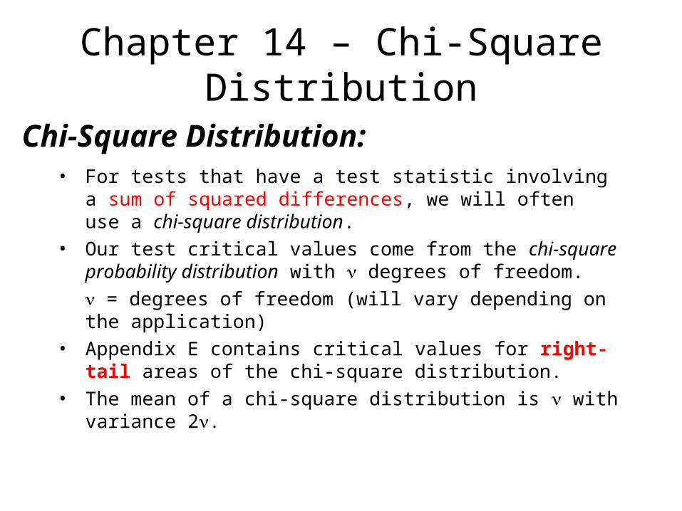
Chapter 14 – Chi-Square Distribution
• For tests that have a test statistic involving a sum of squared differences, we will often use a chi-square distribution.
• Our test critical values come from the chi-square probability distribution with degrees of freedom.
= degrees of freedom (will vary depending on the application)
• Appendix E contains critical values for right-tail areas of the chi-square distribution.
• The mean of a chi-square distribution is with variance 2.
Chi-Square Distribution:
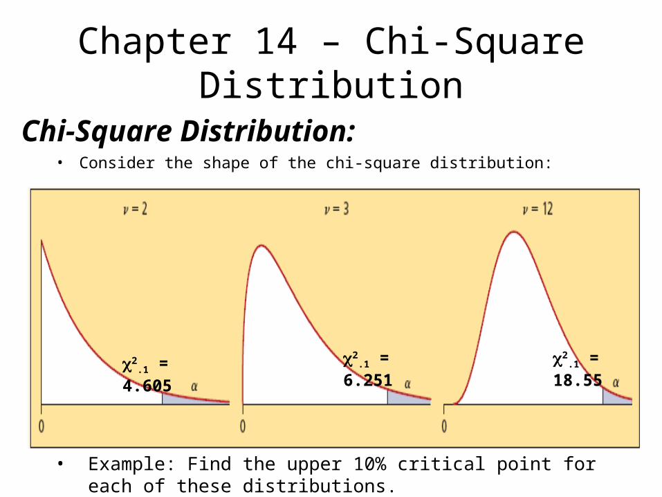
Chapter 14 – Chi-Square Distribution
• Consider the shape of the chi-square distribution:
Chi-Square Distribution:
• Example: Find the upper 10% critical point for each of these distributions.
2.1 = 4.605 2
.1 = 6.251 2.1 = 18.55
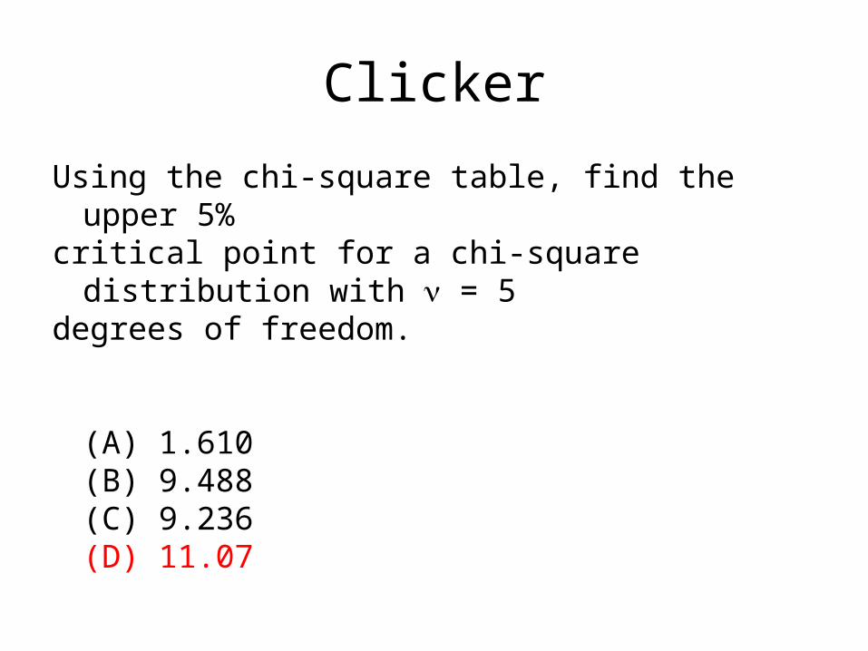
Clicker
Using the chi-square table, find the upper 5% critical point for a chi-square distribution with = 5 degrees of freedom.
(A) 1.610(B) 9.488(C) 9.236(D) 11.07
Chapter 14 – Chi-Square Test for Independence
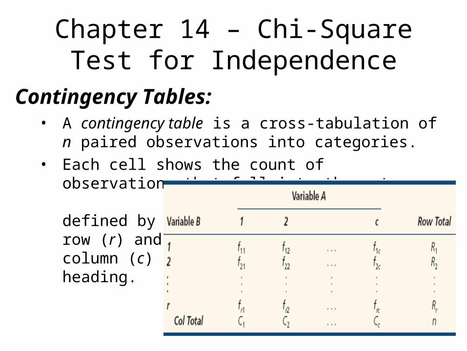
• A contingency table is a cross-tabulation of n paired observations into categories.
• Each cell shows the count of observations that fall into the category defined by its row (r) and column (c)heading.
Contingency Tables:
Chapter 14 – Chi-Square Test for Independence
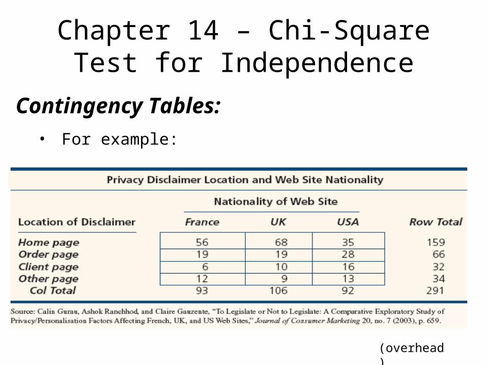
Contingency Tables:
• For example:
(overhead)
Chapter 14 – Chi-Square Test for Independence
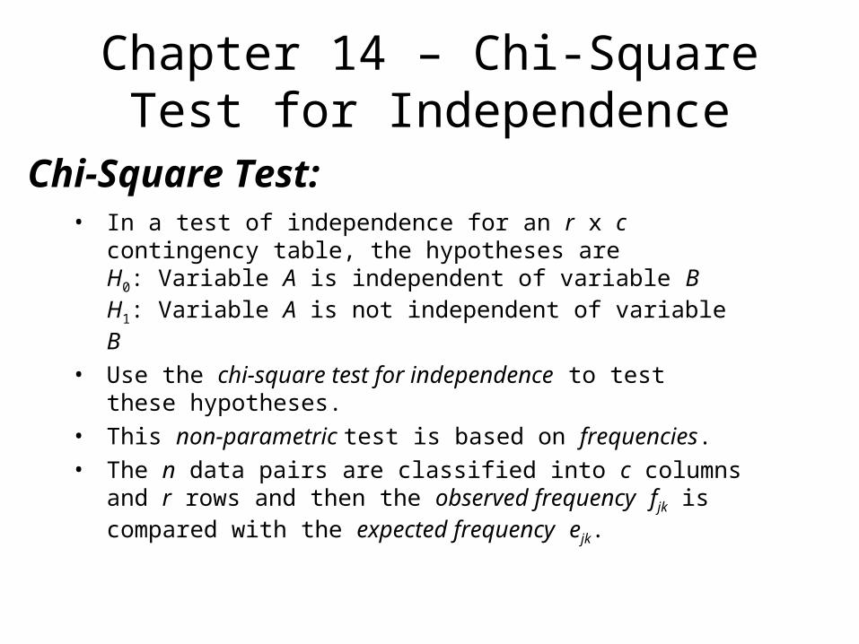
Chi-Square Test:• In a test of independence for an r x c contingency
table, the hypotheses areH0: Variable A is independent of variable BH1: Variable A is not independent of variable B
• Use the chi-square test for independence to test these hypotheses.
• This non-parametric test is based on frequencies.• The n data pairs are classified into c columns and
r rows and then the observed frequency fjk is compared with the expected frequency ejk.

Chapter 14 – Chi-Square Test for Independence
• The critical value comes from the chi-square probability distribution with degrees of freedom.
= degrees of freedom = (r – 1)(c – 1)where r = number of rows in the table
c = number of columns in the table
Chi-Square Distribution:
Chapter 14 – Chi-Square Test for Independence
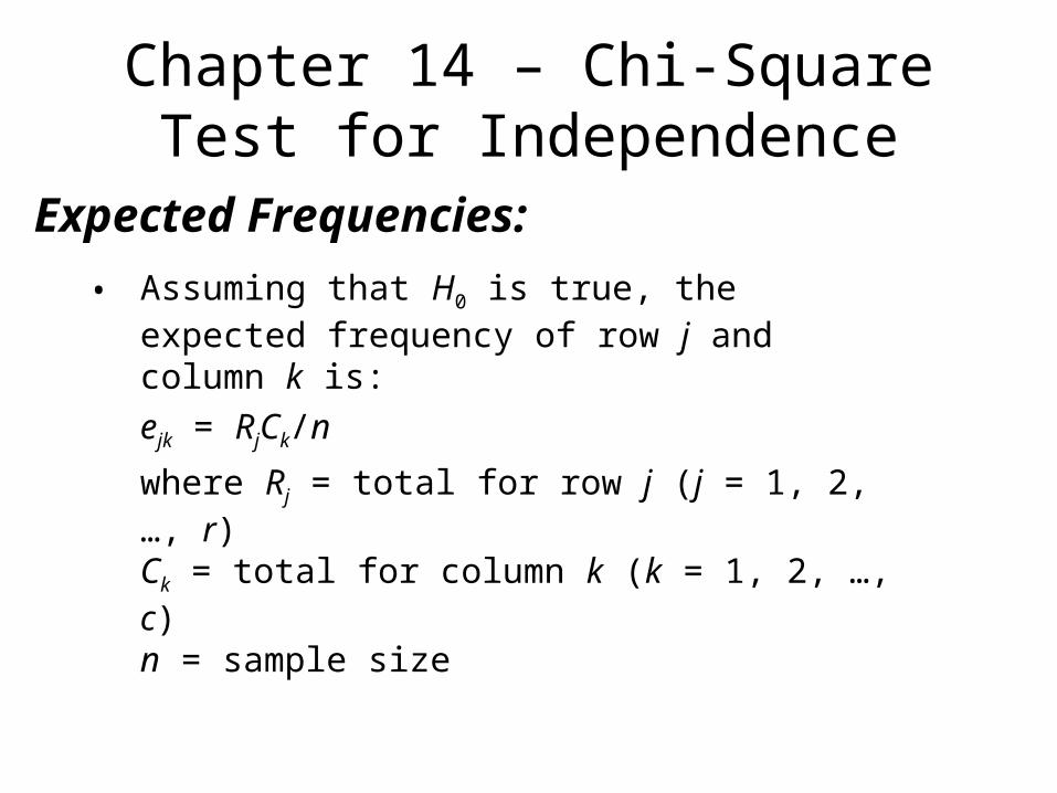
• Assuming that H0 is true, the expected frequency of row j and column k is:
ejk = RjCk/n
where Rj = total for row j (j = 1, 2, …, r)
Ck = total for column k (k = 1, 2, …, c)
n = sample size
Expected Frequencies:
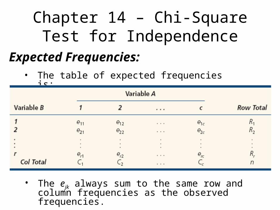
Chapter 14 – Chi-Square Test for Independence
• The table of expected frequencies is:
• The ejk always sum to the same row and column frequencies as the observed frequencies.
Expected Frequencies:

Chapter 14 – Chi-Square Test for Independence
• Step 1: State the Hypotheses
H0: Variable A is independent of variable B
H1: Variable A is not independent of variable B
• Step 2: State the Decision Rule
Calculate = (r – 1)(c – 1)
For a given , look up the right-tail critical value (2
) from Appendix E or by using Excel.
Reject H0 if test statistic > 2 (or if p-value < ).
Steps in Testing the Hypotheses:
Chapter 14 – Chi-Square Test for Independence
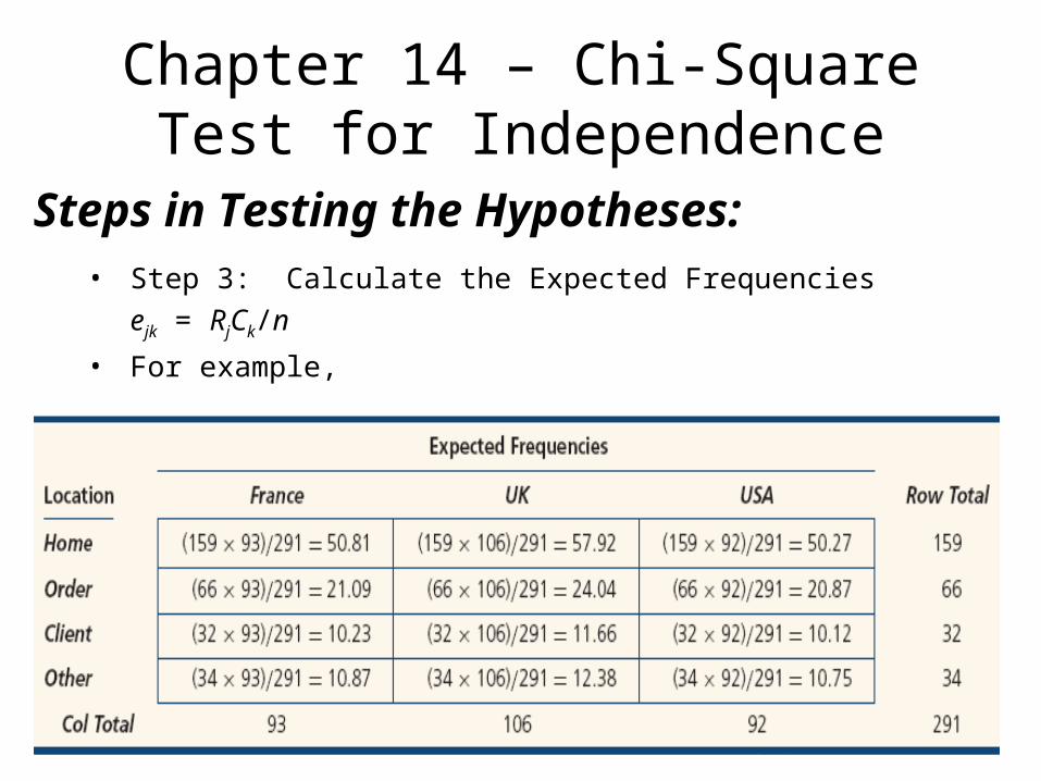
• Step 3: Calculate the Expected Frequencies
ejk = RjCk/n
• For example,
Steps in Testing the Hypotheses:
Chapter 14 – Chi-Square Test for Independence
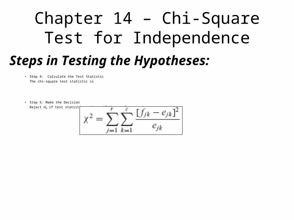
• Step 4: Calculate the Test Statistic
The chi-square test statistic is
• Step 5: Make the Decision
Reject H0 if test statistic > 2 or if the p-value < .
Steps in Testing the Hypotheses:
Chapter 14 – Chi-Square Test for Independence
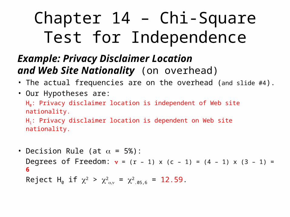
Example: Privacy Disclaimer Location and Web Site Nationality (on overhead)• The actual frequencies are on the overhead (and slide #4).• Our Hypotheses are:
H0: Privacy disclaimer location is independent of Web site nationality.
H1: Privacy disclaimer location is dependent on Web site nationality.
• Decision Rule (at = 5%):
Degrees of Freedom: = (r – 1) x (c – 1) = (4 – 1) x (3 – 1) = 6
Reject H0 if 2 > 2 = 2
.05,6 = 12.59.
Chapter 14 – Chi-Square Test for Independence
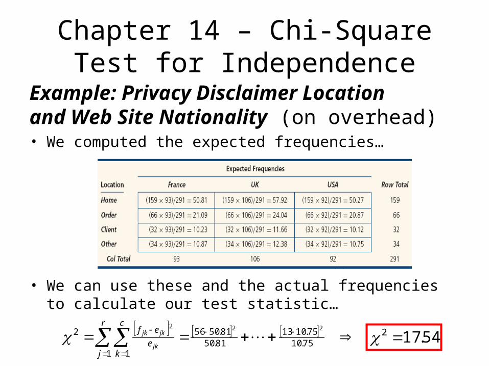
Example: Privacy Disclaimer Location and Web Site Nationality (on overhead)• We computed the expected frequencies…
• We can use these and the actual frequencies to calculate our test statistic…
75.1075.1013
81.5081.5056
1 1
2 222
r
j
c
ke
ef
jk
jkjk 54.172
Clickers
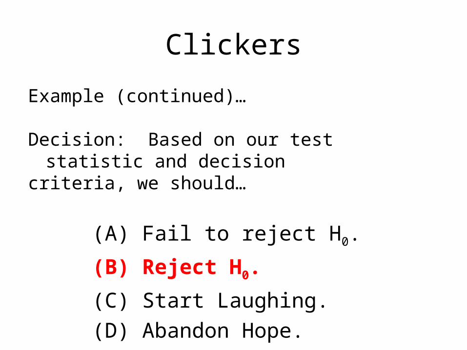
Example (continued)…
Decision: Based on our test statistic and decision criteria, we should…
(A) Fail to reject H0.
(B) Reject H0.
(C) Start Laughing.
(D) Abandon Hope.
Chapter 14 – Chi-Square Test for Independence
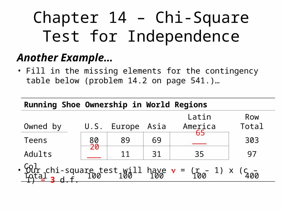
Another Example…• Fill in the missing elements for the contingency table
below (problem 14.2 on page 541.)…
• Our chi-square test will have = (r – 1) x (c – 1) = 3 d.f.
Running Shoe Ownership in World Regions
Owned by U.S. Europe Asia Latin America Row Total
Teens 80 89 69 ___ 303
Adults ___ 11 31 35 97
Col Total 100 100 100 100 400
20
65

Chapter 14 – Chi-Square Test for Independence
Running Shoe Ownership in World Regions (Actual Frequencies)
Owned by U.S. Europe Asia Latin America Row Total
Teens 80 89 69 65 303
Adults 20 11 31 35 97
Col Total 100 100 100 100 400
Running Shoe Ownership in World Regions (Expected Frequencies)
Owned by U.S. Europe Asia Latin America Row Total
Teens 75.75 75.75 75.75 (303x100)/400 = 75.75 303
Adults 24.25 24.25 24.25 (97x100)/400 = 24.25 97
Col Total 100 100 100 100 400
Chapter 14 – Chi-Square Test for Independence
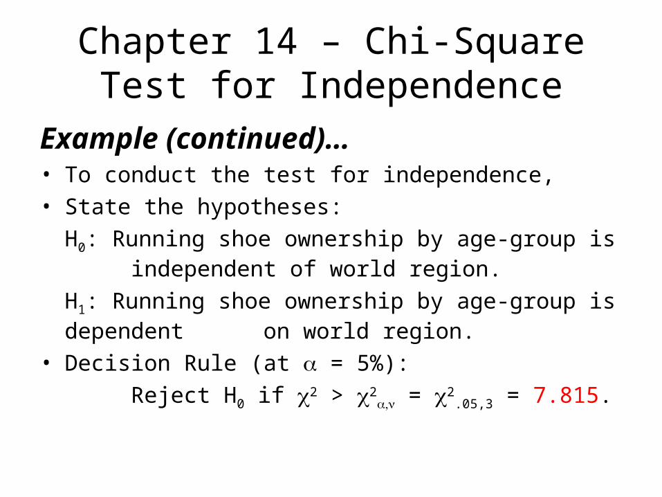
Example (continued)…• To conduct the test for independence,• State the hypotheses:
H0: Running shoe ownership by age-group is independent of world region.
H1: Running shoe ownership by age-group is dependent on world region.
• Decision Rule (at = 5%):
Reject H0 if 2 > 2 = 2
.05,3 = 7.815.
Clickers
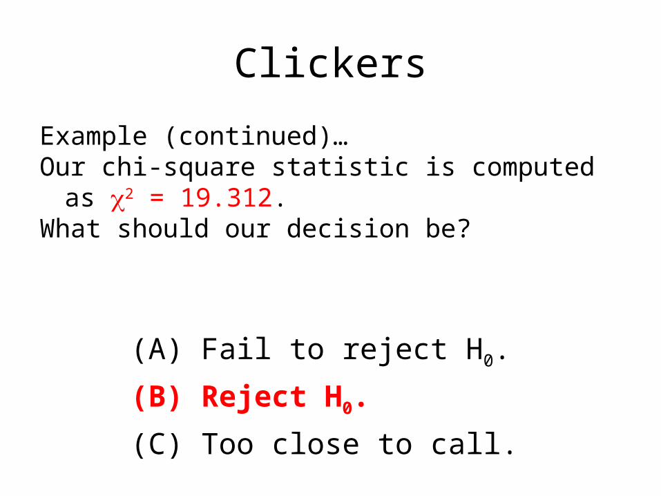
Example (continued)…Our chi-square statistic is computed as 2 = 19.312.What should our decision be?
(A) Fail to reject H0.
(B) Reject H0.
(C) Too close to call.
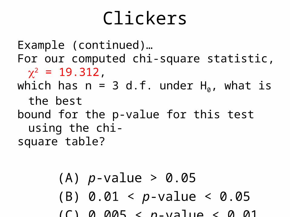
ClickersExample (continued)…For our computed chi-square statistic, 2 = 19.312,which has n = 3 d.f. under H0, what is the best bound for the p-value for this test using the chi-square table?
(A) p-value > 0.05
(B) 0.01 < p-value < 0.05
(C) 0.005 < p-value < 0.01
(D) p-value < 0.005
Chapter 14 – Chi-Square Test for Goodness-of-Fit
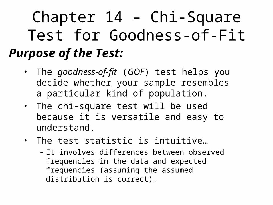
Purpose of the Test:
• The goodness-of-fit (GOF) test helps you decide whether your sample resembles a particular kind of population.
• The chi-square test will be used because it is versatile and easy to understand.
• The test statistic is intuitive…– It involves differences between observed frequencies in
the data and expected frequencies (assuming the assumed distribution is correct).
Chapter 14 – Chi-Square Test for Goodness-of-Fit
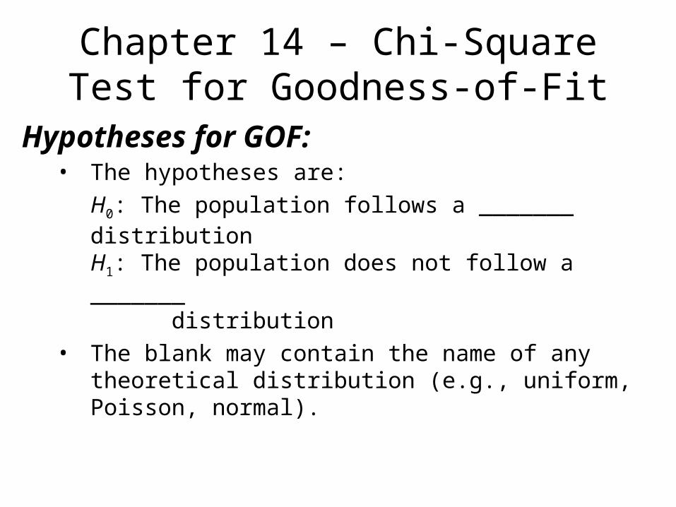
Hypotheses for GOF:• The hypotheses are:
H0: The population follows a _______ distributionH1: The population does not follow a _______ distribution
• The blank may contain the name of any theoretical distribution (e.g., uniform, Poisson, normal).
Chapter 14 – Chi-Square Test for Goodness-of-Fit
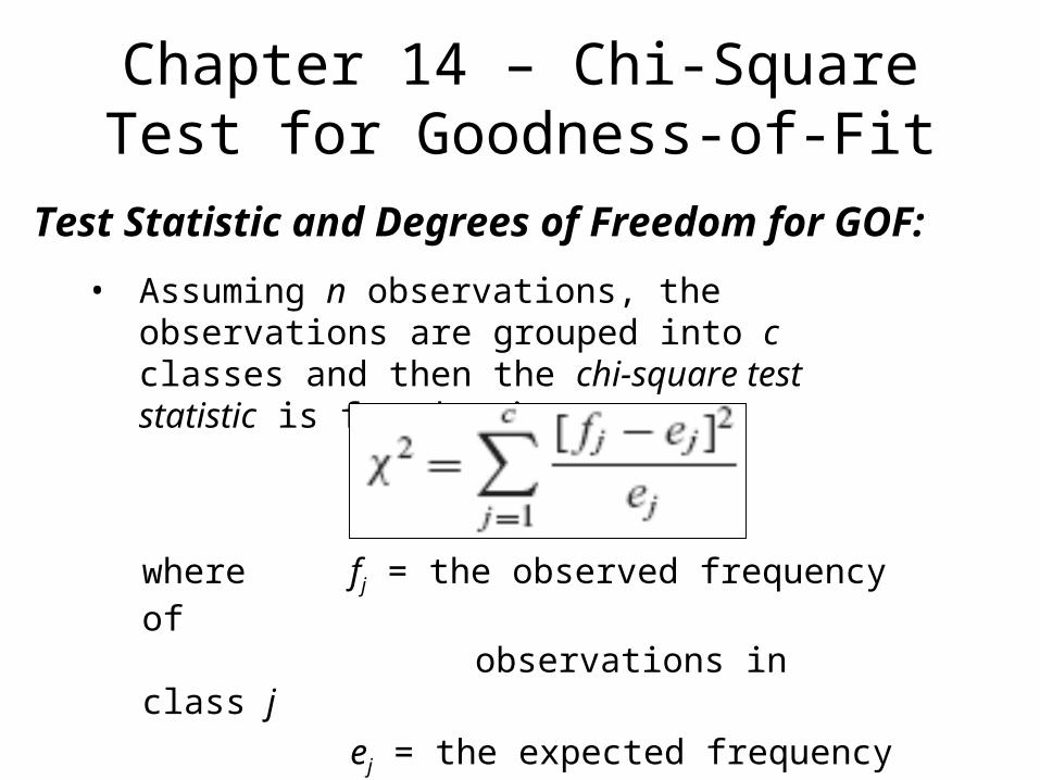
Test Statistic and Degrees of Freedom for GOF:
• Assuming n observations, the observations are grouped into c classes and then the chi-square test statistic is found using:
where fj = the observed frequency of observations in class j
ej = the expected frequency in class j if
H0 were true
Chapter 14 – Chi-Square Test for Goodness-of-Fit
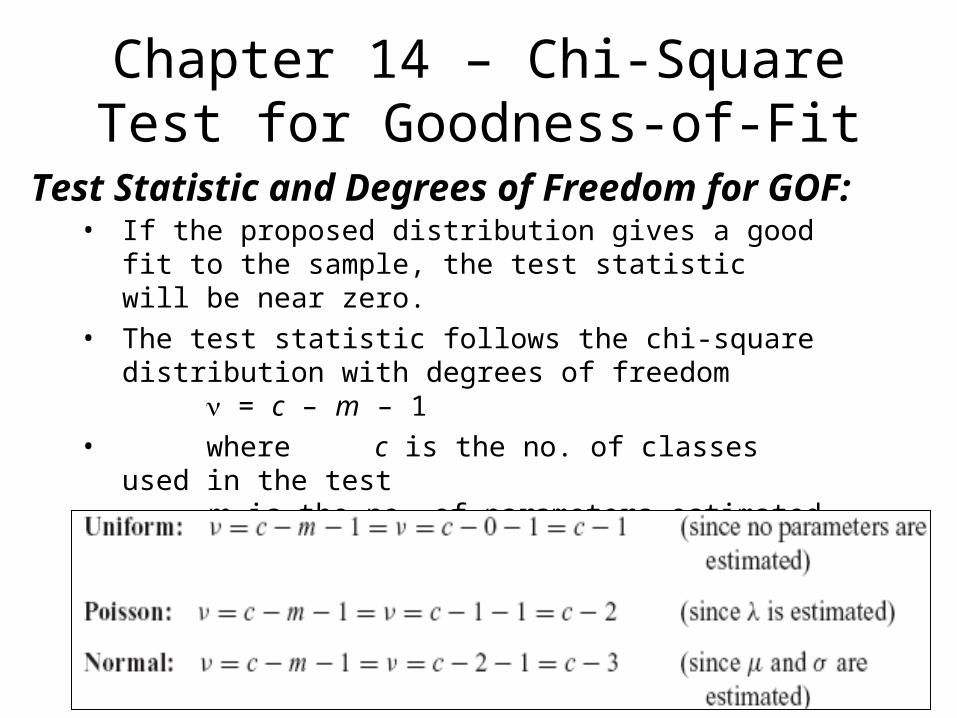
Test Statistic and Degrees of Freedom for GOF:• If the proposed distribution gives a good fit to the
sample, the test statistic will be near zero.• The test statistic follows the chi-square
distribution with degrees of freedom = c – m – 1
• where c is the no. of classes used in the test
m is the no. of parameters estimated
Chapter 14 – Chi-Square Test for Goodness-of-Fit
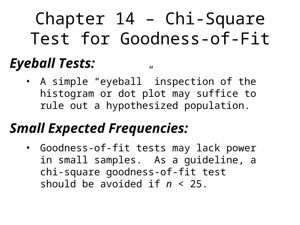
• A simple “eyeball” inspection of the histogram or dot plot may suffice to rule out a hypothesized population.
Eyeball Tests:
• Goodness-of-fit tests may lack power in small samples. As a guideline, a chi-square goodness-of-fit test should be avoided if n < 25.
Small Expected Frequencies:
Chapter 14 – Chi-Square Test for Goodness-of-Fit
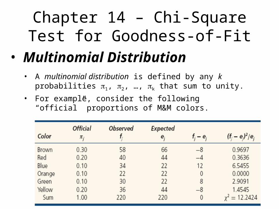
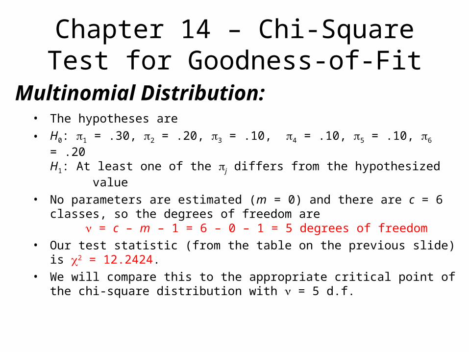
• A multinomial distribution is defined by any k probabilities 1, 2, …, k that sum to unity.
• For example, consider the following “official” proportions of M&M colors.
• Multinomial Distribution
Chapter 14 – Chi-Square Test for Goodness-of-Fit
• The hypotheses are
• H0: 1 = .30, 2 = .20, 3 = .10, 4 = .10, 5 = .10, 6 = .20H1: At least one of the j differs from the hypothesized value
• No parameters are estimated (m = 0) and there are c = 6 classes, so the degrees of freedom are
= c – m – 1 = 6 – 0 – 1 = 5 degrees of freedom • Our test statistic (from the table on the previous slide) is 2 =
12.2424.• We will compare this to the appropriate critical point of the chi-
square distribution with = 5 d.f.
Multinomial Distribution:
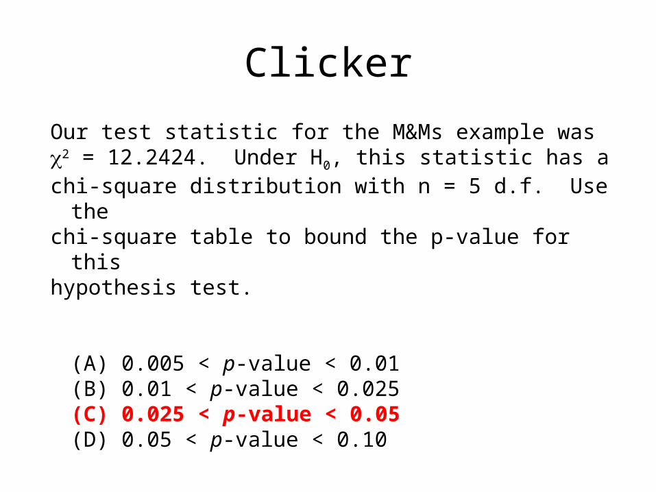
Clicker
Our test statistic for the M&Ms example was 2 = 12.2424. Under H0, this statistic has a chi-square distribution with n = 5 d.f. Use the chi-square table to bound the p-value for this hypothesis test.
(A) 0.005 < p-value < 0.01(B) 0.01 < p-value < 0.025(C) 0.025 < p-value < 0.05(D) 0.05 < p-value < 0.10
Chapter 14 – Chi-Square Test for Goodness-of-Fit
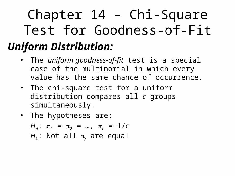
• The uniform goodness-of-fit test is a special case of the multinomial in which every value has the same chance of occurrence.
• The chi-square test for a uniform distribution compares all c groups simultaneously.
• The hypotheses are:
H0: 1 = 2 = …, c = 1/cH1: Not all j are equal
Uniform Distribution:
Chapter 14 – Chi-Square Test for Goodness-of-Fit
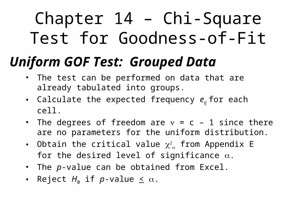
• The test can be performed on data that are already tabulated into groups.
• Calculate the expected frequency eij for each cell.
• The degrees of freedom are = c – 1 since there are no parameters for the uniform distribution.
• Obtain the critical value from Appendix E for the
desired level of significance .• The p-value can be obtained from Excel.
• Reject H0 if p-value < .
Uniform GOF Test: Grouped Data
Chapter 14 – Chi-Square Test for Goodness-of-Fit
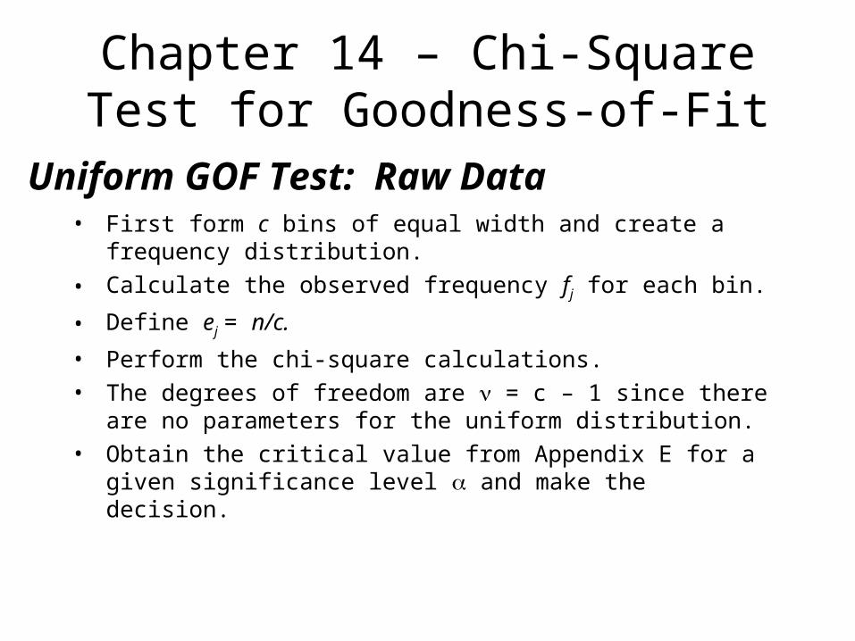
• First form c bins of equal width and create a frequency distribution.
• Calculate the observed frequency fj for each bin.
• Define ej = n/c.
• Perform the chi-square calculations.• The degrees of freedom are = c – 1 since there are
no parameters for the uniform distribution.• Obtain the critical value from Appendix E for a given
significance level and make the decision.
Uniform GOF Test: Raw Data
Chapter 14 – Chi-Square Test for Goodness-of-Fit
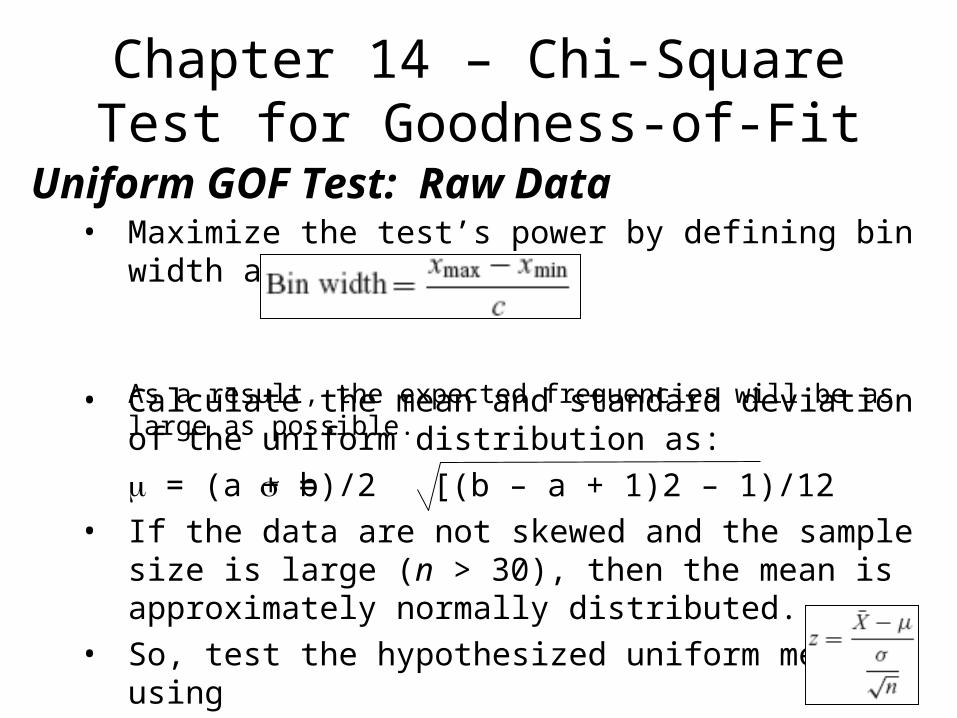
• Maximize the test’s power by defining bin width as
As a result, the expected frequencies will be as large as possible.
Uniform GOF Test: Raw Data
• Calculate the mean and standard deviation of the uniform distribution as:
= (a + b)/2• If the data are not skewed and the sample size is large
(n > 30), then the mean is approximately normally distributed.
• So, test the hypothesized uniform mean using
= [(b – a + 1)2 – 1)/12
Chapter 14 – Chi-Square Test for Goodness-of-Fit
General GOF Tests:• Goodness-of-Fit tests can be constructed in a similar
manner for other distributions (Poisson, Normal, etc.)• We will generally conduct these tests using a software
package.