Beam Test of CCDs for Vertex detectors of JLC

SHIRASAKI Yasuhiro

August 27, 1999

1 Introduction

The standard model of elementary particle physics has been verified withmany experiments in these 30 years. The last quark so-called “top” wasfound by the Fermi laboratory experiment of the year 1994 in U.S.A withthe accelerator TeVatron.

The Joint Linear Collider (hereafter JLC) is in the planning stage as lin-ear electron-positron collider of the next generation, for the energy frontiersof elementary particle physics. The JLC is planned to generate any heavyparticles, like a higgs or super symmetry particles, to verify the standardmodel with the above TeV total energy of e+e−. It is very hard to recon-struct tracks decayed from such short life-time particles. Therefore vertexdetectors are necessary to determine the decay points of b/b̄, c/c̄ with highspatial resolution.

For the advanced detection of decay points, CCD is powerful candidatefor vertex tracker in these days. Recent semiconductor processing technologyimprovement achieved to manufacture the high resolution detectors. Theadvantage of CCD is unambiguous reconstruction capability, less occupancyand less multiple scattering, when compared with silicon strip detectors.

As a precedent for an application of CCD vertex detector, SLAC LargeDetector experiment has been carried out successfully. In the experimentthey used the CCDs at near 180K. The thermal shrink rate difference be-tween CCD and backing structures occur complex spatial distortion at suchlow temperature. It made some measurement errors in charged particletracking. Cooling structures also caused more multiple scattering and lowerresolution.

On the other hand, we will simplify cooling system and operate CCDsin near root temperature to reduce distortions of detectors and multiplescattering in our plan.

1.1 Measurement of spatial resolution

In the past experiments, we operated the full frame type CCD on the marketin the so-called MPP mode at near the room temperature and measured S/N

1

ratio with 55Fe 5.9 KeV X-ray source. It achieved sufficient S/N.We measured incoming angle dependencies of spatial resolution for 3

kinds of CCDs in this study.

2 Experimental setup

The CCDs are exposed to π particles extracted from 12 GeV KEK-PS inT1 line from Jun. 15 to 22 in 1999.

2.1 Sensors

Two kinds of S5466 manufactured by Hamamatsu photonics and CCD02-06by EEV are tested in this study. One S5466 has 10 µm of epitaxial layer,the another has 50 µm of it. (Table1)

CCD HPK S5466 EEV(10um) (50um) CCD02-06

Effective area 512 × 512 ← 385 × 578Pixel Pitch 24 µm ← 22 µmChip size 12.2882 mm2 ← 8.47 × 12.716 mm2

Epitaxial Layer 10 µm 50 µm 20 µmAmp. Sensitivity 2.0µV/e ← 1.0µV/e

Table 1: Specifications of CCDs

Each of CCD sensor is mounted upon the Al2O3 body.

2.2 Setup

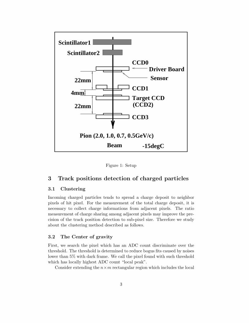
Three reference sensors and one target sensor are kept in a constant tem-perature box at several near room temperatures. In this study, data takenat -15C◦ is used. Coincidence of two monitoring plastic scintillaters placedin front of target sensors are used to count passing charged particles (Fig1).

The special chip which have no Al2O3 behind a sensor is used as secondlayer (CCD1) to avoid multiple Coulomb scattering effect. The sensors ofCCD0 and CCD1 faces downstream side, that of CCD2 and CCD3 facesupstream side for the same reason. Therefore multiple Coulomb scatteringcaused with Al2O3 are negligible.

The detector is exposed to 2.0, 1.0, 0.7 and 0.5 GeV/c minimum ionizedparticles (MIPs, π−). The angles of beam incidence to sensors are kept to0◦, 45◦ and 60◦ (Fig19).

2

-15degC

Driver BoardSensor

22mm

4mm

22mm

CCD0

Target CCD

Pion (2.0, 1.0, 0.7, 0.5GeV/c)

CCD1

(CCD2)

CCD3

Scintillator2

Scintillator1

Beam

Figure 1: Setup

3 Track positions detection of charged particles

3.1 Clustering

Incoming charged particles tends to spread a charge deposit to neighborpixels of hit pixel. For the measurement of the total charge deposit, it isnecessary to collect charge informations from adjacent pixels. The ratiomeasurement of charge sharing among adjacent pixels may improve the pre-cision of the track position detection to sub-pixel size. Therefore we studyabout the clustering method described as follows.

3.2 The Center of gravity

First, we search the pixel which has an ADC count discriminate over thethreshold. The threshold is determined to reduce bogus fits caused by noiseslower than 5% with dark frame. We call the pixel found with such thresholdwhich has locally highest ADC count “local peak”.

Consider extending the n×m rectangular region which includes the local

3

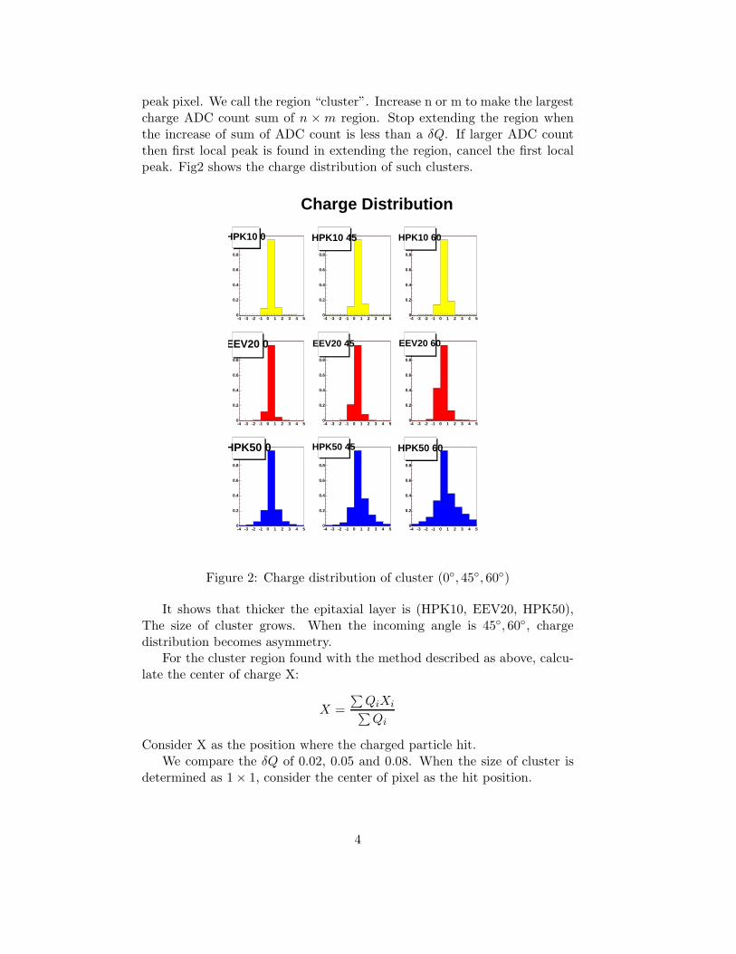
peak pixel. We call the region “cluster”. Increase n or m to make the largestcharge ADC count sum of n ×m region. Stop extending the region whenthe increase of sum of ADC count is less than a δQ. If larger ADC countthen first local peak is found in extending the region, cancel the first localpeak. Fig2 shows the charge distribution of such clusters.

-4 -3 -2 -1 0 1 2 3 4 50

0.2

0.4

0.6

0.8

1HPK10 0

-4 -3 -2 -1 0 1 2 3 4 50

0.2

0.4

0.6

0.8

1HPK10 45

-4 -3 -2 -1 0 1 2 3 4 50

0.2

0.4

0.6

0.8

1HPK10 60

-4 -3 -2 -1 0 1 2 3 4 50

0.2

0.4

0.6

0.8

1EEV20 0

-4 -3 -2 -1 0 1 2 3 4 50

0.2

0.4

0.6

0.8

1EEV20 45

-4 -3 -2 -1 0 1 2 3 4 50

0.2

0.4

0.6

0.8

1EEV20 60

-4 -3 -2 -1 0 1 2 3 4 50

0.2

0.4

0.6

0.8

1HPK50 0

-4 -3 -2 -1 0 1 2 3 4 50

0.2

0.4

0.6

0.8

1HPK50 45

-4 -3 -2 -1 0 1 2 3 4 50

0.2

0.4

0.6

0.8

1HPK50 60

Charge Distribution

Figure 2: Charge distribution of cluster (0◦, 45◦, 60◦)

It shows that thicker the epitaxial layer is (HPK10, EEV20, HPK50),The size of cluster grows. When the incoming angle is 45◦, 60◦, chargedistribution becomes asymmetry.

For the cluster region found with the method described as above, calcu-late the center of charge X:

X =∑

QiXi∑Qi

Consider X as the position where the charged particle hit.We compare the δQ of 0.02, 0.05 and 0.08. When the size of cluster is

determined as 1× 1, consider the center of pixel as the hit position.

4

3.3 correction

With the finding method of the hit position described as above, the pro-jection of positions to X axis shows a periodical distribution which has thesame size of CCD pixels (Fig 3).

0 0.5 1 1.5 2 2.5 3 3.5 4 4.5 50

100

200

300

400

500

HPK10_NX_1869Nent = 18076 Mean = 2.544RMS = 1.433

HPK10_NX_1869 HPK10_NX_1869Nent = 18076 Mean = 2.544RMS = 1.433

Figure 3: The center of clusters with linear sum. colored has a cluster sizeof 1× 1

Since incoming beam has no periodical density which size is same to thepixel size and it should has uniformity, potential wall of CCD prevents todiffuse the generated charge and might cause the periodical distribution inthe fig 3.

Therefore assuming the uniform incoming particles, we correct the posi-tion X calculated with the linear charge sum. It may improve the precisionof the position. Assuming the uniformity (dN

dX =constant), we do the cor-rection:

r = [X + 1]−X

δ(r) =1N

∫ r

0

dN

dxdx

X ′ = X − r + δ(r)

Fig4 shows rough uniformity of corrected positions. Since colored pixelsin the histogram which has 1 × 1 cluster size is never affected with thecorrection, the histogram has small peaks of such pixels.

3.4 Ratio Location Mapping

Choose the maximum ADC count sum of four 2× 2 square regions in 3× 3region which has a local peak at its center. We assume it is the clustercandidate.

5

0 0.5 1 1.5 2 2.5 3 3.5 4 4.5 50

50

100

150

200

250

300

350

400

450

HPK10_AX_1869Nent = 18076 Mean = 2.504RMS = 1.433

HPK10_AX_1869 HPK10_AX_1869Nent = 18076 Mean = 2.504RMS = 1.433

Figure 4: The center of clusters with linear sum and correction. colored hasa cluster size of 1× 1

With the ADC count ratio of local peak and adjacent pixel Rx anduniformity of incoming particles,

dN

dx= const, Rx =

Cnext

Cpeak

follows

X(log(R)) =0.5N

∫ log(R)

−∞dN

d log(r)d log(r)

=∞∑

n=0

an logn(R)

determine the expand coefficients with real data. Using the expanded func-tion, we calculated positions of each cluster (Fig 5). We used approximatedfunction 5th order (Fig 6). For example the function for HPK10µm, 60◦

X(r) = (0.64± 0.08) + (0.51± 0.10)r − (0.13± 0.15)r2 − (0.14± 0.09)r3

+(0.03± 0.06)r4 + (0.02± 0.03)r5

(r = logR).Expand coefficients has incidence angle dependency. The figure shows

that charge sharing is not uniformly, when the incidence angle is not vertical.

4 Alignment

4.1 Residual

Determine the spatial resolutions with CCD0, CCD1 and CCD2. CCD3 isused to check the bogus tracks.

6

(Direction) ×(log 10Rx)-3 -2 -1 0 1 2 3

Pos

ition

0

0.2

0.4

0.6

0.8

1

HPK10

Linear

0

60

45

Charge share

c0 c0 c0 c0 c0 c0 c0c0 c0c1 c1 c1 c1 c1 c1 c1 c1 c1

Figure 5: RLM Mapping function

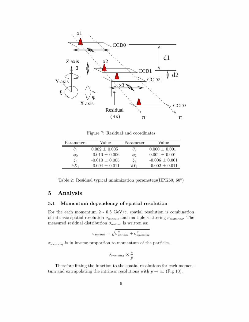
Find the intersection point for linear extension of cluster on the CCD0to that on the CCD1 and CCD2 surface. Define the difference between thatintersection point and clusters on CCD2 as residual (Fig 7).

If CCD0, CCD1 and CCD2 are parallel to each other, residual is showedwith the distance between CCD0 and CCD1 (d1) and that of CCD1 andCCD2 (d2):

Residual = x3−{

x2 +d2d1

(x2− x1)}

We used rectangular coordinates and set the center of CCD1 as the origin(Fig 7).

4.2 Rough alignment

First, we assume all the detectors are parallel to align roughly. We plot therelative position of clusters on CCDn (n = 0, 2, 3) to the cluster positionson CCD1 and find the peaks determine large gap in X-Y plane:

δXi = Xi −X1(i = 0, 2, 3)

After that, determine Z directional displacement with:

Z =X2 −X1

X1 −X0

7

-3 -2 -1 0 1 2 30

0.2

0.4

0.6

0.8

11st degree: Chisq = 16.43

Rx0

-3 -2 -1 0 1 2 30

0.2

0.4

0.6

0.8

1 3rd degree: Chisq = 0.69

Rx1

-3 -2 -1 0 1 2 30

0.2

0.4

0.6

0.8

1 5th degree: Chisq = 0.10

Rx2

-3 -2 -1 0 1 2 30

0.2

0.4

0.6

0.8

17th degree: Chisq = 0.04

Rx3

Figure 6: RLM Mapping approximation

Determine the rotation on the X-Y plane with the correlations of dx−Yand dy −X.

4.3 Track Selection

With the rough alignment described as above, we find particle track candi-dates in certain reliability. Since the distance ratio of CCD1 - CCD2 andCCD1 - CCD3 is about 1:5, We assume the track which has the smaller resid-ual on CCD3 than five times of residual extent on CCD2 (σ) as candidates(Fig 8).

4.4 Residual Minimization

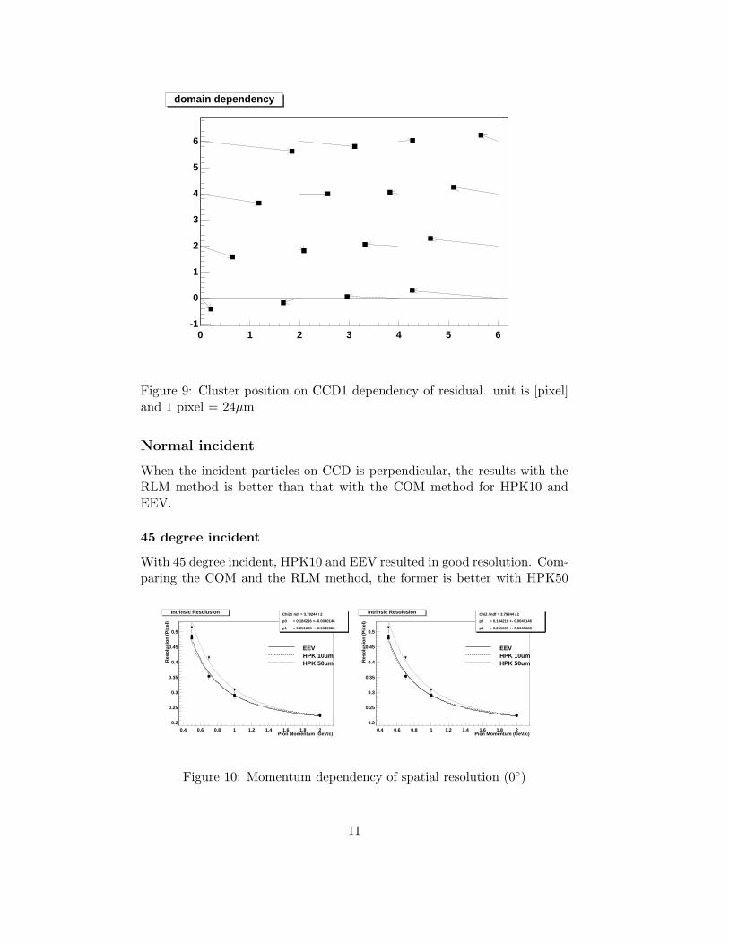
When we split the track candidates to the 4× 4 region groups with clusterposition on the CCD1 and plotted residuals. The histogram in the Fig 9shows an rule based mean value transition.

The tilt of CCD planes against reference CCD might caused such tran-sitions. We assume CCD0 and CCD2 has rotations against CCD1 and min-imize square sum of residuals with the parameters as follows (Fig 7):

x′

y′

z′

= (θ) (φ) (ξ)

xy0

Table 2 shows typical minimized parameters.

8

(Rx)

������������

������������

��������

������������

ππ

CCD1

CCD2

CCD3

CCD0

X axisResidual

φ

Z axis

ξ

Y axis

θ

d1

d2

x1

x2

x3

Figure 7: Residual and coordinates

Parameters Value Parameter Valueθ0 0.002 ± 0.005 θ2 0.000 ± 0.001φ0 -0.010 ± 0.006 φ2 0.002 ± 0.001ξ0 -0.010 ± 0.005 ξ2 -0.006 ± 0.001

δX1 -0.094 ± 0.011 δY1 -0.002 ± 0.011

Table 2: Residual typical minimization parameters(HPK50, 60◦)

5 Analysis

5.1 Momentum dependency of spatial resolution

For the each momentum 2 - 0.5 GeV/c, spatial resolution is combinationof intrinsic spatial resolution σintrinsic and multiple scattering σscattering. Themeasured residual distribution σresidual is written as:

σresidual =√

σ2intrinsic + σ2

scattering

σscattering is in inverse proportion to momentum of the particles.

σscattering ∝ 1p

Therefore fitting the function to the spatial resolutions for each momen-tum and extrapolating the intrinsic resolutions with p→∞ (Fig 10).

9

CCD2

σ

5σ

cluster

cluster

CCD0

CCD1

CCD3

Figure 8: assume the track which has the smaller residual on CCD3 thanfive times of residual extent on CCD2 (σ) as candidates

σresidual is combination of all the resolutions for each CCD and showed:

σ2residual = σ2

CCD2 + (1 + Z)2σ2CCD1 + Z2σ2

CCD0

Here Z is d2d1 . When we used HPK10 target CCD, we assumed:

σCCD0 = σCCD1 = σCCD2

It worked out the intrinsic resolution for each CCD.

5.2 Intrinsic resolution

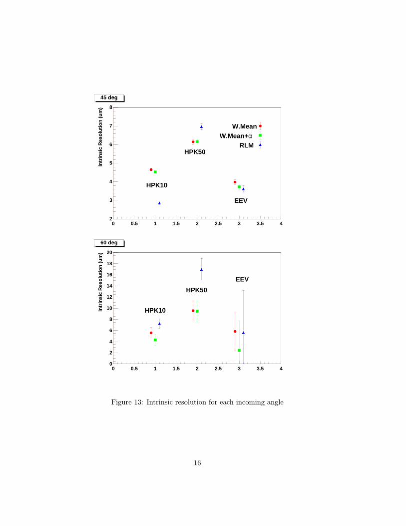
Table 3, 4, 5, Fig 13 show intrinsic resolutions for each incoming angle andCCDs.

CCD Resolution (µm)Center Of Mass RLM

HPK 10 3.87 ± 0.05 2.98 ± 0.05HPK 50 2.35 ± 0.10 2.26 ± 0.19EEV 20 3.90 ± 0.12 2.73 ± 0.30

Table 3: 0◦

10

0 1 2 3 4 5 6-1

0

1

2

3

4

5

6

domain dependency

Figure 9: Cluster position on CCD1 dependency of residual. unit is [pixel]and 1 pixel = 24µm

Normal incident

When the incident particles on CCD is perpendicular, the results with theRLM method is better than that with the COM method for HPK10 andEEV.

45 degree incident

With 45 degree incident, HPK10 and EEV resulted in good resolution. Com-paring the COM and the RLM method, the former is better with HPK50

Pion Momentum (GeV/c)0.4 0.6 0.8 1 1.2 1.4 1.6 1.8 2

Res

olus

ion

(Pix

el)

0.2

0.25

0.3

0.35

0.4

0.45

0.5

Chi2 / ndf = 1.17771 / 2

p0 = 0.194841 +- 0.00462799

p1 = 0.216988 +- 0.00750747

Chi2 / ndf = 1.34979 / 2

p0 = 0.201219 +- 0.00360035

p1 = 0.211187 +- 0.00628146

Chi2 / ndf = 3.79244 / 2

p0 = 0.184216 +- 0.0040146

p1 = 0.251655 +- 0.0049686

EEVHPK 10umHPK 50um

Intrinsic Resolusion Chi2 / ndf = 3.79244 / 2

p0 = 0.184216 +- 0.0040146

p1 = 0.251655 +- 0.0049686

Pion Momentum (GeV/c)0.4 0.6 0.8 1 1.2 1.4 1.6 1.8 2

Res

olus

ion

(Pix

el)

0.2

0.25

0.3

0.35

0.4

0.45

0.5

Chi2 / ndf = 1.17771 / 2

p0 = 0.194841 +- 0.00462799

p1 = 0.216988 +- 0.00750747

Chi2 / ndf = 1.34979 / 2

p0 = 0.201219 +- 0.00360035

p1 = 0.211187 +- 0.00628146

Chi2 / ndf = 3.79244 / 2

p0 = 0.184216 +- 0.0040146

p1 = 0.251655 +- 0.0049686

EEVHPK 10umHPK 50um

Intrinsic Resolusion Chi2 / ndf = 3.79244 / 2

p0 = 0.184216 +- 0.0040146

p1 = 0.251655 +- 0.0049686

Figure 10: Momentum dependency of spatial resolution (0◦)

11

Momentum (GeV/c)0.5 1 1.5 2 2.5

Res

olut

ion

(pix

el)

0.3

0.4

0.5

0.6

0.7

0.8

0.9

1

X resolution

HPK10

HPK50

EEV

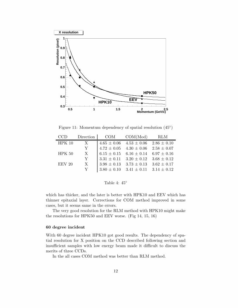
Figure 11: Momentum dependency of spatial resolution (45◦)

CCD Direction COM COM(Mod) RLMHPK 10 X 4.65 ± 0.06 4.53 ± 0.06 2.86 ± 0.10

Y 4.72 ± 0.05 4.30 ± 0.06 2.58 ± 0.07HPK 50 X 6.15 ± 0.15 6.16 ± 0.14 6.97 ± 0.16

Y 3.31 ± 0.11 3.20 ± 0.12 3.68 ± 0.12EEV 20 X 3.98 ± 0.13 3.73 ± 0.13 3.62 ± 0.17

Y 3.80 ± 0.10 3.41 ± 0.11 3.14 ± 0.12

Table 4: 45◦

which has thicker, and the later is better with HPK10 and EEV which hasthinner epitaxial layer. Corrections for COM method improved in somecases, but it seems same in the errors.

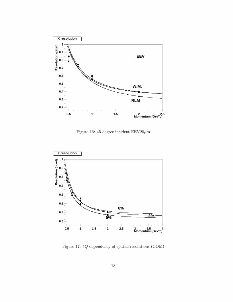
The very good resolution for the RLM method with HPK10 might makethe resolutions for HPK50 and EEV worse. (Fig 14, 15, 16)

60 degree incident

With 60 degree incident HPK10 got good results. The dependency of spa-tial resolution for X position on the CCD described following section andinsufficient samples with low energy beam made it difficult to discuss themerits of three CCDs.

In the all cases COM method was better than RLM method.

12

Momentum (GeV/c)0.5 1 1.5 2 2.5

Res

olut

ion

(pix

el)

0.5

1

1.5

2

2.5

3

3.5

4

X resolution

EEV

HPK10

HPK50

Figure 12: Momentum dependency of spatial resolution (60◦)

CCD Direction COM COM(Mod) RLMHPK 10 X 5.60 ± 0.92 4.33 ± 0.98 7.27 ± 0.85

Y 5.40 ± 0.34 5.34 ± 0.36 4.61 ± 0.30HPK 50 X 9.58 ± 1.71 9.47 ± 1.89 16.97 ± 1.92

Y 5.12 ± 0.72 4.79 ± 0.71 3.61 ± 0.83EEV 20 X 5.85 ± 3.52 2.47 ± 5.27 5.67 ± 7.51

Y 6.68 ± 0.91 6.76 ± 1.09 3.48 ± 1.12

Table 5: 60◦

5.3 The center of mass method and the ratio location map-ping method

Dynamic determination of the cluster size for the COM method with itscharge distribution got good result than the RLM method which uses only2 × 2 region when the charge extend more than three pixels. HPK50 with45 degree incident and all the CCDs with 60 degree incident is in such case.

On the other hand, the RLM method is better because it is sensitive forfine charge ratio change when most charge is stay in the 2× 2 region.

5.4 Cluster threshold dependency of spatial resolution

The spatial resolutions with the COM method may depend on the clusteringthreshold. The threshold determines how extent the clusters. We stopped

13

for extension when the total charge change for extension is (δQ) smallerthan 2% as mentioned above.

We changed the threshold 2%, 5%, and 8% and got the following result.Table 6 and figure 17 shows the result. 5% of threshold got the best resultand 8% of it is worse. Anyway the change of the resolution is not so large.

δQ X [pixel] Y [pixel]2% 0.35 ± 0.01 0.27 ± 0.015% 0.33 ± 0.01 0.23 ± 0.018% 0.37 ± 0.01 0.30 ± 0.01

Table 6: δQ dependency of spatial resolutions (HPK50, 45degree)

5.5 The track passing position dependency

In this experiment, spatial resolution had a position dependency for X di-rection of CCD for each momentum. Figure 18 shows typical example. aquarter of left region is worse.

The reason might that CCD has the size of 12mm2 but the hole in theceramics package is 10mm2. The incident particles passing out of hole mightbe scattered with the ceramics package.(Fig19).

Therefore we checked the intrinsic resolutions without the tracks whichpass the left half of the CCD (Fig 20, Table 7).

CCD direction COM COM (w/ correction) RLMHPK 10 X 4.73 ± 0.08 4.56 ± 0.10 3.30 ± 0.06

Y 4.64 ± 0.07 4.53 ± 0.09 2.57 ± 0.05HPK 50 X 6.56 ± 0.17 6.68 ± 0.18 6.92 ± 0.14

Y 4.44 ± 0.14 4.39 ± 0.16 3.79 ± 0.10EEV 20 X 4.72 ± 0.18 5.05 ± 0.19 4.37 ± 0.16

Y 5.70 ± 0.15 4.87 ± 0.18 3.34 ± 0.13

Table 7: 45◦ (left half of CCD, HPK10

The result shows that the intrinsic resolutions are not different. Withthe EEV, as it has three fourth size of HPK, the exclusion of right halfcaused the lack of samples.

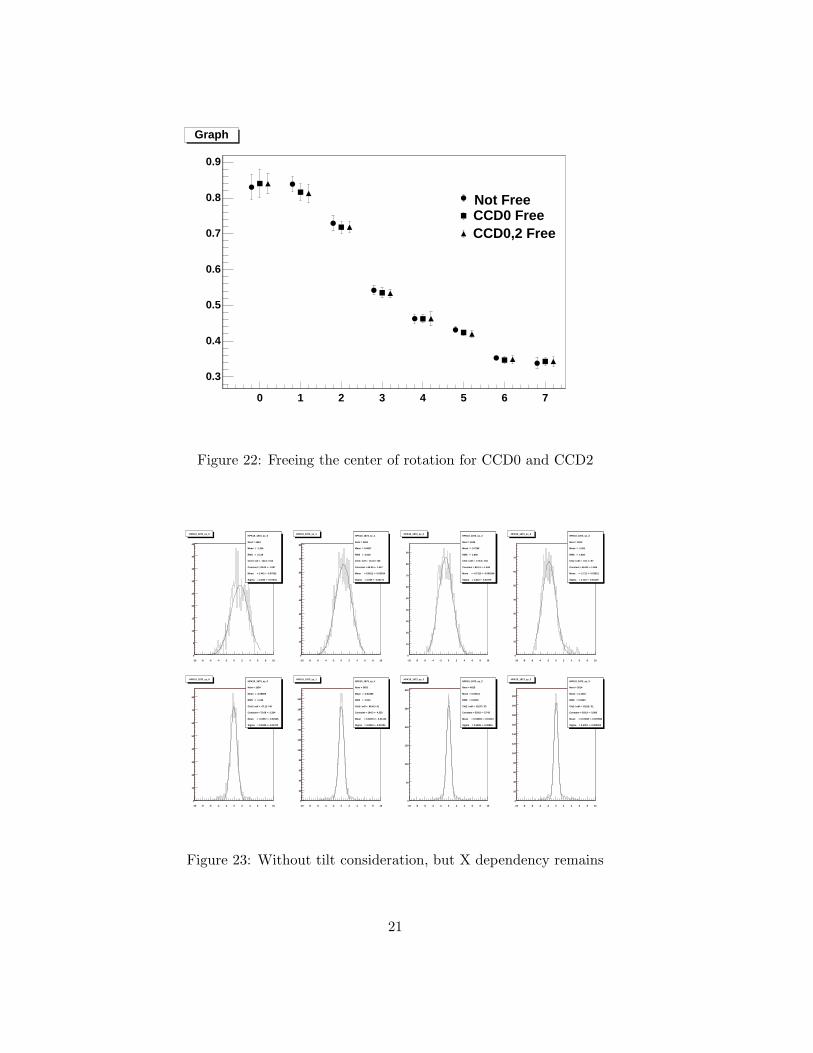
Figure 21 shows residual distribution for HPK50 and 60 degree incidentwith left half, right half or all the tracks. Figure 22 shows the case freeingthe center of rotation for CCD0 and CCD2.

In any case the residual distribution did not change.

14

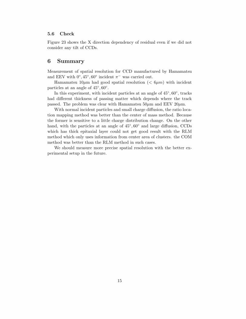
5.6 Check

Figure 23 shows the X direction dependency of residual even if we did notconsider any tilt of CCDs.

6 Summary

Measurement of spatial resolution for CCD manufactured by Hamamatsuand EEV with 0◦, 45◦, 60◦ incident π− was carried out.

Hamamatsu 10µm had good spatial resolution (< 6µm) with incidentparticles at an angle of 45◦, 60◦.

In this experiment, with incident particles at an angle of 45◦, 60◦, trackshad different thickness of passing matter which depends where the trackpassed. The problem was clear with Hamamatsu 50µm and EEV 20µm.

With normal incident particles and small charge diffusion, the ratio loca-tion mapping method was better than the center of mass method. Becausethe former is sensitive to a little charge distribution change. On the otherhand, with the particles at an angle of 45◦, 60◦ and large diffusion, CCDswhich has thick epitaxial layer could not get good result with the RLMmethod which only uses information from center area of clusters. the COMmethod was better than the RLM method in such cases.

We should measure more precise spatial resolution with the better ex-perimental setup in the future.

15

0 0.5 1 1.5 2 2.5 3 3.5 4

Intr

insi

c R

esol

utio

n (u

m)

2

3

4

5

6

7

8

45 deg

HPK10

HPK50

EEV

W.MeanW.Mean+α

RLM

0 0.5 1 1.5 2 2.5 3 3.5 4

Intr

insi

c R

esol

utio

n (u

m)

0

2

4

6

8

10

12

14

16

18

20

60 deg

HPK10

HPK50

EEV

Figure 13: Intrinsic resolution for each incoming angle

16

Momentum (GeV/c)0.5 1 1.5 2 2.5

Res

olut

ion

(pix

el)

0.2

0.3

0.4

0.5

0.6

0.7

0.8

0.9

1

X resolution

RLM

W.M.

W.M.+α

HPK10

Figure 14: 45 degree incident HPK10µm

Momentum (GeV/c)0.5 1 1.5 2 2.5

Res

olut

ion

(pix

el)

0.2

0.3

0.4

0.5

0.6

0.7

0.8

0.9

1

X resolution

RLM

W.M.

Figure 15: 45 degree incident HPK50µm

17

Momentum (GeV/c)0.5 1 1.5 2 2.5

Res

olut

ion

(pix

el)

0.2

0.3

0.4

0.5

0.6

0.7

0.8

0.9

1

X resolution

RLM

W.M.

EEV

Figure 16: 45 degree incident EEV20µm

Momentum (GeV/c)0.5 1 1.5 2 2.5 3 3.5 4

Res

olut

ion

(pix

el)

0.3

0.4

0.5

0.6

0.7

0.8

0.9

1

X resolution

5%

8%

2%

Figure 17: δQ dependency of spatial resolutions (COM)

18

Region (X direction)-1 0 1 2 3 4 5 6 7 8

Res

olut

ion

(pix

el)

0.2

0.4

0.6

0.8

1

1.2

1.4

1.6

1.8

2

Resolution

60 deg X

60 deg Y

45 deg

0 deg

Figure 18: Position dependency of spatial resolution (2GeV/c)

影響を受ける部分

Figure 19: The tracks scattered by the ceramics package

19

Momentum (GeV/c)0.5 1 1.5 2 2.5 3

Res

olut

ion

(pix

el)

0.5

1

1.5

2

2.5

Y resolution

Left half

Right half

Entire

Figure 20: Spatial resolutions with the tracks passing left half, right half,and all tracks

0 1 2 3 4 5 6 7

0.3

0.4

0.5

0.6

0.7

0.8

0.9

Graph

AllLeft halfRight half

Figure 21: Spatial resolution with left half tracks, right half tracks and allof them

20

0 1 2 3 4 5 6 7

0.3

0.4

0.5

0.6

0.7

0.8

0.9

Graph

Not FreeCCD0 FreeCCD0,2 Free

Figure 22: Freeing the center of rotation for CCD0 and CCD2

-10 -8 -6 -4 -2 0 2 4 6 8 10

0

5

10

15

20

25

30

35

40

45

HPK10_1873_sx_0

Nent = 1654

Mean = 1.154

RMS = 2.119

Chi2 / ndf = 132.4 / 102

Constant = 28.02 +- 1.007

Mean = 1.441 +- 0.07922

Sigma = 2.285 +- 0.07444

HPK10_1873_sx_0HPK10_1873_sx_0

Nent = 1654

Mean = 1.154

RMS = 2.119

Chi2 / ndf = 132.4 / 102

Constant = 28.02 +- 1.007

Mean = 1.441 +- 0.07922

Sigma = 2.285 +- 0.07444

-10 -8 -6 -4 -2 0 2 4 6 8 10

0

10

20

30

40

50

60

70

80

HPK10_1873_sx_1

Nent = 3453

Mean = 0.4807

RMS = 2.019

Chi2 / ndf = 112.6 / 105

Constant = 65.25 +- 1.447

Mean = 0.5511 +- 0.03934

Sigma = 2.069 +- 0.03171

HPK10_1873_sx_1HPK10_1873_sx_1

Nent = 3453

Mean = 0.4807

RMS = 2.019

Chi2 / ndf = 112.6 / 105

Constant = 65.25 +- 1.447

Mean = 0.5511 +- 0.03934

Sigma = 2.069 +- 0.03171

-10 -8 -6 -4 -2 0 2 4 6 8 10

0

10

20

30

40

50

60

70

80

90

HPK10_1873_sx_2

Nent = 4025

Mean = -0.7294

RMS = 1.866

Chi2 / ndf = 170.6 / 104

Constant = 85.12 +- 1.544

Mean = -0.7313 +- 0.005249

Sigma = 1.813 +- 0.01575

HPK10_1873_sx_2HPK10_1873_sx_2

Nent = 4025

Mean = -0.7294

RMS = 1.866

Chi2 / ndf = 170.6 / 104

Constant = 85.12 +- 1.544

Mean = -0.7313 +- 0.005249

Sigma = 1.813 +- 0.01575

-10 -8 -6 -4 -2 0 2 4 6 8 10

0

10

20

30

40

50

60

70

HPK10_1873_sx_3

Nent = 3014

Mean = -1.551

RMS = 1.883

Chi2 / ndf = 161.1 / 97

Constant = 66.58 +- 1.655

Mean = -1.711 +- 0.03621

Sigma = 1.722 +- 0.03119

HPK10_1873_sx_3HPK10_1873_sx_3

Nent = 3014

Mean = -1.551

RMS = 1.883

Chi2 / ndf = 161.1 / 97

Constant = 66.58 +- 1.655

Mean = -1.711 +- 0.03621

Sigma = 1.722 +- 0.03119

-10 -8 -6 -4 -2 0 2 4 6 8 10

0

10

20

30

40

50

60

70

80

HPK10_1873_sy_0

Nent = 1654

Mean = -0.09869

RMS = 1.136

Chi2 / ndf = 67.12 / 49

Constant = 72.08 +- 2.334

Mean = -0.0507 +- 0.02226

Sigma = 0.8429 +- 0.01702

HPK10_1873_sy_0HPK10_1873_sy_0

Nent = 1654

Mean = -0.09869

RMS = 1.136

Chi2 / ndf = 67.12 / 49

Constant = 72.08 +- 2.334

Mean = -0.0507 +- 0.02226

Sigma = 0.8429 +- 0.01702

-10 -8 -6 -4 -2 0 2 4 6 8 10

0

20

40

60

80

100

120

140

160

180

200

HPK10_1873_sy_1

Nent = 3453

Mean = -0.04386

RMS = 1.013

Chi2 / ndf = 98.42 / 41

Constant = 184.5 +- 4.352

Mean = 0.00674 +- 0.01133

Sigma = 0.6912 +- 0.01094

HPK10_1873_sy_1HPK10_1873_sy_1

Nent = 3453

Mean = -0.04386

RMS = 1.013

Chi2 / ndf = 98.42 / 41

Constant = 184.5 +- 4.352

Mean = 0.00674 +- 0.01133

Sigma = 0.6912 +- 0.01094

-10 -8 -6 -4 -2 0 2 4 6 8 10

0

50

100

150

200

250

300

HPK10_1873_sy_2

Nent = 4025

Mean = 0.05101

RMS = 0.9278

Chi2 / ndf = 92.97 / 33

Constant = 259.8 +- 5.743

Mean = 0.04369 +- 0.01013

Sigma = 0.5689 +- 0.00855

HPK10_1873_sy_2HPK10_1873_sy_2

Nent = 4025

Mean = 0.05101

RMS = 0.9278

Chi2 / ndf = 92.97 / 33

Constant = 259.8 +- 5.743

Mean = 0.04369 +- 0.01013

Sigma = 0.5689 +- 0.00855

-10 -8 -6 -4 -2 0 2 4 6 8 10

0

20

40

60

80

100

120

140

160

180

200

220

HPK10_1873_sy_3

Nent = 3014

Mean = 0.1232

RMS = 0.9643

Chi2 / ndf = 62.82 / 31

Constant = 203.9 +- 3.986

Mean = 0.07498 +- 0.007988

Sigma = 0.5367 +- 0.002263

HPK10_1873_sy_3HPK10_1873_sy_3

Nent = 3014

Mean = 0.1232

RMS = 0.9643

Chi2 / ndf = 62.82 / 31

Constant = 203.9 +- 3.986

Mean = 0.07498 +- 0.007988

Sigma = 0.5367 +- 0.002263

Figure 23: Without tilt consideration, but X dependency remains

21