1

Beam vibrations: Discrete mass and stiffness models

Ana Cláudia Sousa Neves ana.neves@tecnico.ulisboa.pt

Instituto Superior Técnico, Universidade de Lisboa, Portugal May, 2015

Abstract

In the present work the dynamic behavior of several beams with different support conditions, forced or in free vibration, is studied. Using the Discrete Element Method (DEM), the expressions governing the motion of the blocks in which the beam is discretized are derived. A MATLAB program that calculates natural frequencies and mode shapes is developed; the results are then compared with the exact solutions, in order to validate the models. The program also allows to simulate the evolution of the dynamic systems in time, yielding displacements, velocities and accelerations. The effect on the beam behavior due to the introduction of one or more cracks is analyzed; cracks with different sizes and positions are considered. Three distinctive cases for the studied models are considered: non-existence of cracks, permanently open cracks or “breathing cracks” (cracks that open and close depending on the curvature sign). The obtained results are shown with the help of tables and graphics and, when possible, compared with the exact solutions or with numerical or experimental results found in literature.

Key-words: vibration of beams, rigid blocks, discrete stiffness, breathing crack.

1. Introduction

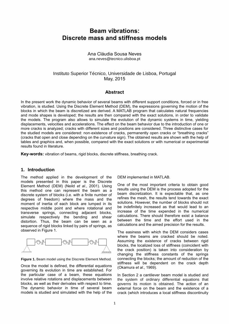
The method applied in the development of the models presented in this paper is the Discrete Element Method (DEM) (Neild et al., 2001). Using this method one can represent the beam as a discrete system of blocks (i.e. with a finite number of degrees of freedom) where the mass and the moment of inertia of each block are lumped in its respective middle point and where rotational and transverse springs, connecting adjacent blocks, simulate respectively the bending and shear distortion. Thus, the beam can be seen as a sequence of rigid blocks linked by pairs of springs, as observed in Figure 1.

Figure 1. Beam model using the Discrete Element Method.

Once the model is defined, the differential equations governing its evolution in time are established. For the particular case of a beam, these equations involve relative rotations and displacements between blocks, as well as their derivates with respect to time. The dynamic behavior in time of several beam models is studied and simulated with the help of the

DEM implemented in MATLAB.

One of the most important criteria to obtain good results using the DEM is the process adopted for the beam discretization. It is expectable that, as one refines the mesh, the results tend towards the exact solutions. However, the number of blocks should not be indefinitely increased as that would lead to an increase of the time expended in the numerical calculations. There should therefore exist a balance between the time and the effort used in the calculations and the aimed precision for the results.

The easiness with which the DEM considers cases where the beams are cracked should be noted. Assuming the existence of cracks between rigid blocks, the localized loss of stiffness (coincident with the crack position) is taken into consideration by changing the stiffness constants of the springs connecting the blocks; the amount of reduction of the stiffness will be dependent on the crack depth (Okamura et al., 1969).

In Section 2 a cantilever beam model is studied and the system of ordinary differential equations that governs its motion is obtained. The action of an external force on the beam and the existence of a crack (which introduces a local stiffness discontinuity

2

in the model) are also considered. The crack is either assumed to be always open or to behave like a breathing crack (a crack that opens and closes accordingly to the sign of the curvature of the cross section). The time integration of the equations that govern the motion of a cracked cantilever beam is performed by the Runge-Kutta method and the time evolution of the beam’s dynamic response is presented and compared with experimental results. In Section 3, an analogous study is made for a suspended cracked beam submitted to an oscillatory external force acting perpendicularly to the beam’s suspension plane and free of support conditions in its plane of motion.

The last section is dedicated to the conclusions that result from the performed numerical investigations and to enumerate some aspects that are worth of future attention.

2. Cantilever beam

2.1. Dynamics of a homogeneous

cantilever beam

In this section a cantilever beam of length 𝐿 with

uniform rectangular transverse section 𝑏 × ℎ and

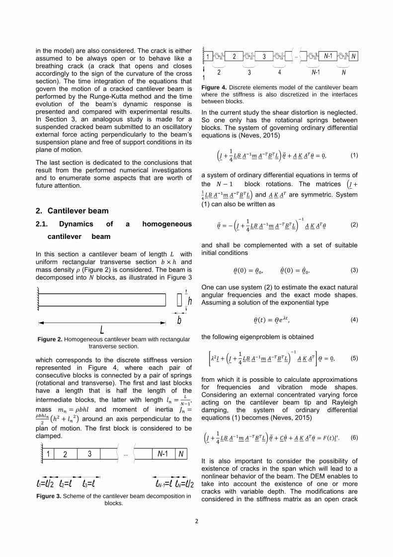
mass density 𝜌 (Figure 2) is considered. The beam is decomposed into 𝑁 blocks, as illustrated in Figure 3

Figure 2. Homogeneous cantilever beam with rectangular

transverse section.

which corresponds to the discrete stiffness version represented in Figure 4, where each pair of consecutive blocks is connected by a pair of springs (rotational and transverse). The first and last blocks have a length that is half the length of the

intermediate blocks, the latter with length 𝑙𝑛 =𝐿

𝑁−1,

mass 𝑚𝑛 = 𝜌𝑏ℎ𝑙 and moment of inertia 𝐽𝑛 =𝜌𝑏ℎ𝑙𝑛

2(ℎ2 + 𝑙𝑛

2) around an axis perpendicular to the

plan of motion. The first block is considered to be clamped.

Figure 3. Scheme of the cantilever beam decomposition in

blocks.

Figure 4. Discrete elements model of the cantilever beam

where the stiffness is also discretized in the interfaces between blocks.

In the current study the shear distortion is neglected. So one only has the rotational springs between blocks. The system of governing ordinary differential equations is (Neves, 2015)

(𝐽 +1

4𝐿𝐵 𝐴−1𝑚 𝐴−𝑇𝐵𝑇𝐿) �� + 𝐴 𝐾 ��𝑇�� = 0, (1)

a system of ordinary differential equations in terms of

the 𝑁 − 1 block rotations. The matrices (𝐽 +1

4𝐿𝐵 𝐴−1𝑚 𝐴−𝑇𝐵𝑇𝐿) and 𝐴 𝐾 ��𝑇 are symmetric. System

(1) can also be written as

�� = − (𝐽 +1

4𝐿𝐵 𝐴−1𝑚 𝐴−𝑇𝐵𝑇𝐿)

−1

𝐴 𝐾 ��𝑇�� (2)

and shall be complemented with a set of suitable initial conditions

��(0) = ��0, ��(0) = ��0. (3)

One can use system (2) to estimate the exact natural angular frequencies and the exact mode shapes. Assuming a solution of the exponential type

��(𝑡) = ��𝑒𝜆𝑡 , (4)

the following eigenproblem is obtained

[𝜆2𝐼 + (𝐽 +1

4𝐿𝐵 𝐴−1𝑚 𝐴−𝑇𝐵𝑇𝐿)

−1

𝐴 𝐾 ��𝑇] �� = 0, (5)

from which it is possible to calculate approximations for frequencies and vibration mode shapes. Considering an external concentrated varying force acting on the cantilever beam tip and Rayleigh damping, the system of ordinary differential equations (1) becomes (Neves, 2015)

(𝐽 +1

4𝐿𝐵 𝐴−1𝑚 𝐴−𝑇𝐵𝑇𝐿) �� + 𝐶�� + 𝐴 𝐾 ��𝑇�� = 𝐹(𝑡)��′. (6)

It is also important to consider the possibility of existence of cracks in the span which will lead to a nonlinear behavior of the beam. The DEM enables to take into account the existence of one or more cracks with variable depth. The modifications are considered in the stiffness matrix as an open crack

3

will produce a stiffness reduction in the section where it is situated.

A cantilever beam with a breathing crack in its upper part, with height 𝑎 and at a distance 𝑥𝑐 from the clamped end is modeled (Figure 5). As the crack is located in the upper part of the beam, when the curvature in that section is positive the crack is assumed to be closed (Figure 6) and there is no discontinuity in flexural stiffness; otherwise, if the curvature in that section is negative the crack is open (Figure 7) and the local stiffness changes. It is assumed that the crack thickness is negligible when compared to its height and that it does not propagate.

Figure 5. Detail of the cantilever beam where the plan

crack of height 𝑎 and width 𝑏 is located.

Figure 6. Closed crack, where 𝜃𝑙 + 𝜃𝑟 = 𝑀𝑙

𝐸𝐼.

Figure 7. Open crack, where 𝜃𝑙 + 𝜃𝑟 = 𝑀 (𝑙

𝐸𝐼+

72

𝐸𝑏ℎ2 𝐹 ( 𝑎

ℎ)).

The stiffness of the spring affected by the crack is determined based in (Okamura et al., 1969). If the cross section has a positive curvature sign, the crack is considered to be closed and the stiffness of the correspondent spring, like the other springs, follows the known expression

𝑘𝑐 =𝐸𝐼

𝑙 (7)

where 𝑙 stands for the length of each block or, equivalently, the length of influence of the 𝑛-th spring. But if the cross section has a negative curvature sign, the crack is considered to be open and the stiffness of the correspondent spring is given by (Okamura et al., 1969)

𝑘𝑐 =1

𝑙𝐸𝐼

+72

𝐸𝑏ℎ2 𝐹 ( 𝑎ℎ) (8)

where

𝐹 ( 𝑎

ℎ) = 1.98 (

𝑎

ℎ)

2

− 3.277 (𝑎

ℎ)

3

+ 14.43 (𝑎

ℎ)

4

−

31.26 (𝑎

ℎ)

5

+ 63.56 (𝑎

ℎ)

6

− 103.36 (𝑎

ℎ)

7

+

147.52 (𝑎

ℎ)

8

− 127.69 (𝑎

ℎ)

9

+ 61.50 (𝑎

ℎ)10

.

(9)

Three models of the cantilever beam were computationally implemented:

2.2. Results

Table 1 shows the geometric and material properties of the cantilever beam.

Table 1. Geometric and material properties of the

cantilever beam.

Geometric properties

𝑏 [m] 0.06

ℎ [m] 0.22

𝐿 [m] 8.0

Material properties

𝐸 [Pa] 210 × 109

𝜌 [kg/m3] 7800

Nonexistence of cracks (the beam has a linear behavior);

An always open crack (the beam also has a linear behavior);

A breathing crack (the beam has a nonlinear behaviour);

4

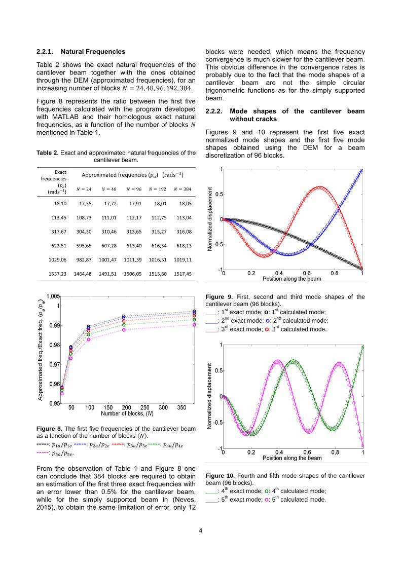
2.2.1. Natural Frequencies

Table 2 shows the exact natural frequencies of the cantilever beam together with the ones obtained through the DEM (approximated frequencies), for an increasing number of blocks 𝑁 = 24, 48, 96, 192, 384.

Figure 8 represents the ratio between the first five frequencies calculated with the program developed with MATLAB and their homologous exact natural frequencies, as a function of the number of blocks 𝑁 mentioned in Table 1.

Table 2. Exact and approximated natural frequencies of the

cantilever beam.

Exact frequencies

(𝑝𝑒) (rads−1)

Approximated frequencies (𝑝𝑎) (rads−1)

𝑁 = 24 𝑁 = 48 𝑁 = 96 𝑁 = 192 𝑁 = 384

18,10 17,35 17,72 17,91 18,01 18,05

113,45 108,73 111,01 112,17 112,75 113,04

317,67 304,30 310,46 313,65 315,27 316,08

622,51 595,65 607,28 613,40 616,54 618,13

1029,06 982,87 1001,47 1011,39 1016,51 1019,11

1537,23 1464,48 1491,51 1506,05 1513,60 1517,45

Figure 8. The first five frequencies of the cantilever beam

as a function of the number of blocks (𝑁).

-----: 𝑝1𝑎/𝑝1𝑒 -----: 𝑝2𝑎/𝑝2𝑒 -----: 𝑝3𝑎/𝑝3𝑒-----: 𝑝4𝑎/𝑝4𝑒

-----: 𝑝5𝑎/𝑝5𝑒 .

From the observation of Table 1 and Figure 8 one can conclude that 384 blocks are required to obtain an estimation of the first three exact frequencies with an error lower than 0.5% for the cantilever beam, while for the simply supported beam in (Neves, 2015), to obtain the same limitation of error, only 12

blocks were needed, which means the frequency convergence is much slower for the cantilever beam. This obvious difference in the convergence rates is probably due to the fact that the mode shapes of a cantilever beam are not the simple circular trigonometric functions as for the simply supported beam.

2.2.2. Mode shapes of the cantilever beam without cracks

Figures 9 and 10 represent the first five exact normalized mode shapes and the first five mode shapes obtained using the DEM for a beam discretization of 96 blocks.

Figure 9. First, second and third mode shapes of the

cantilever beam (96 blocks).

___: 1st exact mode; o: 1

st calculated mode;

___: 2nd

exact mode; o: 2nd

calculated mode;

___: 3rd

exact mode; o: 3rd

calculated mode.

Figure 10. Fourth and fifth mode shapes of the cantilever

beam (96 blocks).

___: 4th

exact mode; o: 4th

calculated mode;

___: 5th

exact mode; o: 5th

calculated mode.

5

Even without an excellent precision, with a discretization of 96 blocks it is already possible to replicate well enough the first three mode shapes. Obviously, by increasing the number of blocks more precise mode shapes would be obtained; but the big improvement achieved for the first five frequencies and modes due to the transition from a low number of blocks to 96 blocks is hardly repeatable if the number of blocks is increased from 96 to more: the approximation improvement is not maintained with an indefinite refinement.

2.2.3. Dynamic evolution of the oscillation of

the cracked cantilever beam

In this section the numerical results obtained using DEM are compared with the results found in the reference (Loutridis et al., 2005) where the only situation considered is that of one breathing crack.

With the purpose of studying the nonlinear response of the cracked cantilever beam, a Plexiglas model with the characteristics found in Table 3 is considered (Loutridis et al., 2005).

Table 3. Geometric and material properties of the

cantilever beam (Loutridis et al., 2005).

Geometric properties

𝑏 [m] 0.02

ℎ [m] 0.02

𝐿 [m] 0.230

Material properties

𝐸 [Pa] 2.5 × 109

𝜌 [kg/m3] 1200

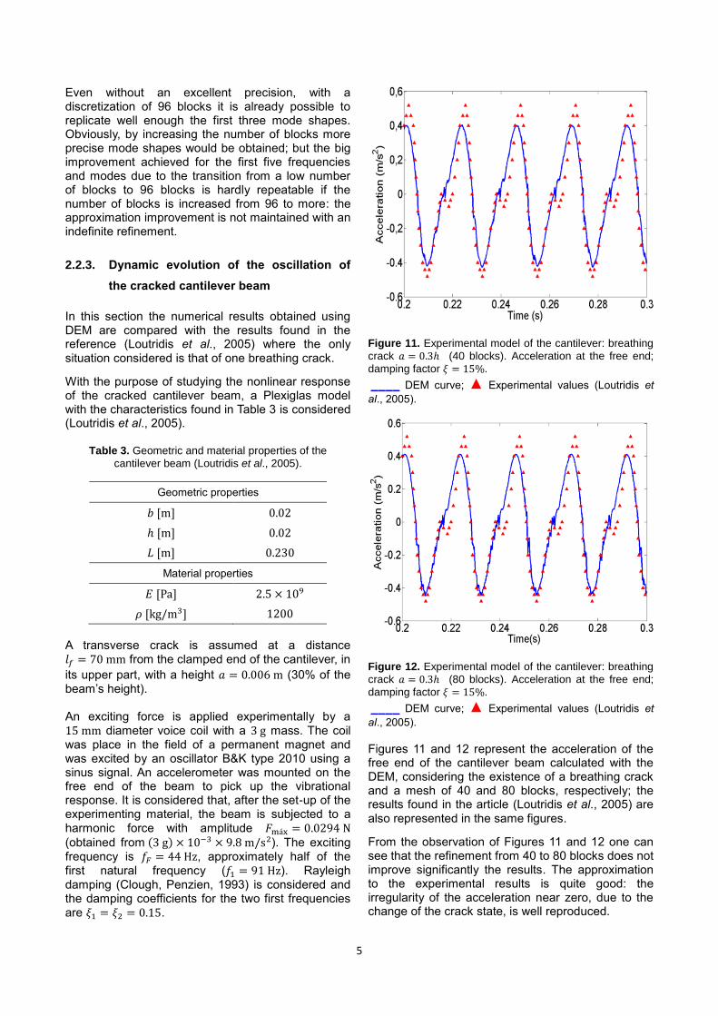
A transverse crack is assumed at a distance 𝑙𝑓 = 70 mm from the clamped end of the cantilever, in

its upper part, with a height 𝑎 = 0.006 m (30% of the beam’s height). An exciting force is applied experimentally by a 15 mm diameter voice coil with a 3 g mass. The coil was place in the field of a permanent magnet and was excited by an oscillator B&K type 2010 using a sinus signal. An accelerometer was mounted on the free end of the beam to pick up the vibrational response. It is considered that, after the set-up of the experimenting material, the beam is subjected to a harmonic force with amplitude 𝐹máx = 0.0294 N

(obtained from (3 g) × 10−3 × 9.8 m/s2). The exciting frequency is 𝑓𝐹 = 44 Hz, approximately half of the first natural frequency (𝑓1 = 91 Hz). Rayleigh damping (Clough, Penzien, 1993) is considered and the damping coefficients for the two first frequencies are 𝜉1 = 𝜉2 = 0.15.

Figure 11. Experimental model of the cantilever: breathing

crack 𝑎 = 0.3ℎ (40 blocks). Acceleration at the free end;

damping factor 𝜉 = 15%.

____ DEM curve; ▲ Experimental values (Loutridis et

al., 2005).

Figure 12. Experimental model of the cantilever: breathing

crack 𝑎 = 0.3ℎ (80 blocks). Acceleration at the free end;

damping factor 𝜉 = 15%.

____ DEM curve; ▲ Experimental values (Loutridis et

al., 2005).

Figures 11 and 12 represent the acceleration of the free end of the cantilever beam calculated with the DEM, considering the existence of a breathing crack and a mesh of 40 and 80 blocks, respectively; the results found in the article (Loutridis et al., 2005) are also represented in the same figures.

From the observation of Figures 11 and 12 one can see that the refinement from 40 to 80 blocks does not improve significantly the results. The approximation to the experimental results is quite good: the irregularity of the acceleration near zero, due to the change of the crack state, is well reproduced.

6

3. Suspended beam

3.1. Dynamics of a homogeneous

suspended beam

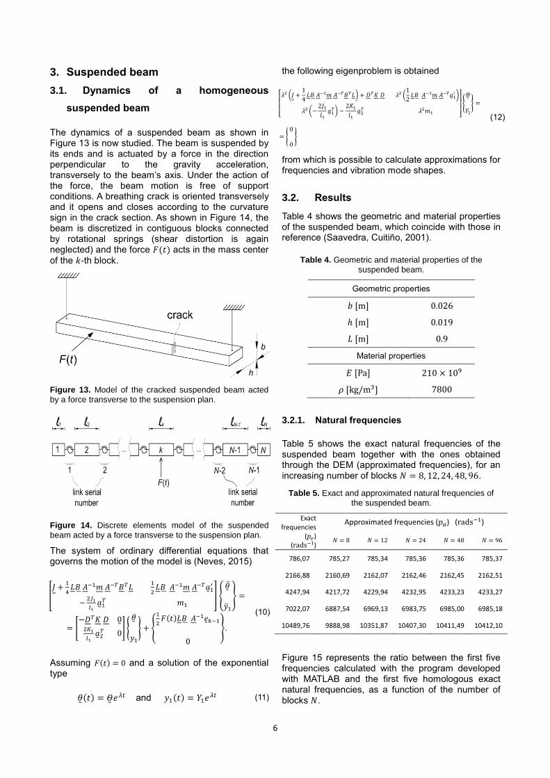
The dynamics of a suspended beam as shown in Figure 13 is now studied. The beam is suspended by its ends and is actuated by a force in the direction perpendicular to the gravity acceleration, transversely to the beam’s axis. Under the action of the force, the beam motion is free of support conditions. A breathing crack is oriented transversely and it opens and closes according to the curvature sign in the crack section. As shown in Figure 14, the beam is discretized in contiguous blocks connected by rotational springs (shear distortion is again neglected) and the force 𝐹(𝑡) acts in the mass center

of the 𝑘-th block.

Figure 13. Model of the cracked suspended beam acted

by a force transverse to the suspension plan.

Figure 14. Discrete elements model of the suspended

beam acted by a force transverse to the suspension plan.

The system of ordinary differential equations that governs the motion of the model is (Neves, 2015)

[𝐽 +

1

4𝐿𝐵 𝐴−1𝑚 𝐴−𝑇𝐵𝑇𝐿

1

2𝐿𝐵 𝐴−1𝑚 𝐴−𝑇��1

′

−2𝐽1

𝑙1��1

𝑇 𝑚1

] {��

��1

} =

= [−𝐷𝑇𝐾 𝐷 0

2𝐾1

𝑙1��2

𝑇 0] {

��

𝑦1

} + {

1

2𝐹(𝑡)𝐿𝐵 𝐴−1��𝑘−1

0

}.

(10)

Assuming 𝐹(𝑡) = 0 and a solution of the exponential type

��(𝑡) = ��𝑒𝜆𝑡 and 𝑦1(𝑡) = 𝑌1𝑒𝜆𝑡 (11)

the following eigenproblem is obtained

[ 𝜆2 (𝐽 +

1

4𝐿𝐵 𝐴−1𝑚 𝐴−𝑇𝐵𝑇𝐿) + 𝐷𝑇𝐾 𝐷 𝜆2 (

1

2𝐿𝐵 𝐴−1𝑚 𝐴−𝑇��1

′ )

𝜆2 (−2𝐽1𝑙1

��1𝑇) −

2𝐾1

𝑙1��2

𝑇 𝜆2𝑚1 ]

{

��

𝑌1

} =

= {0

0}

(12)

from which is possible to calculate approximations for frequencies and vibration mode shapes.

3.2. Results

Table 4 shows the geometric and material properties of the suspended beam, which coincide with those in reference (Saavedra, Cuitiño, 2001).

Table 4. Geometric and material properties of the

suspended beam.

Geometric properties

𝑏 [m] 0.026

ℎ [m] 0.019

𝐿 [m] 0.9

Material properties

𝐸 [Pa] 210 × 109

𝜌 [kg/m3] 7800

3.2.1. Natural frequencies

Table 5 shows the exact natural frequencies of the suspended beam together with the ones obtained through the DEM (approximated frequencies), for an increasing number of blocks 𝑁 = 8, 12, 24, 48, 96.

Table 5. Exact and approximated natural frequencies of

the suspended beam.

Exact frequencies

(𝑝𝑒) (rads−1)

Approximated frequencies (𝑝𝑎) (rads−1)

𝑁 = 8 𝑁 = 12 𝑁 = 24 𝑁 = 48 𝑁 = 96

786,07 785,27 785,34 785,36 785,36 785,37

2166,88 2160,69 2162,07 2162,46 2162,45 2162,51

4247,94 4217,72 4229,94 4232,95 4233,23 4233,27

7022,07 6887,54 6969,13 6983,75 6985,00 6985,18

10489,76 9888,98 10351,87 10407,30 10411,49 10412,10

Figure 15 represents the ratio between the first five frequencies calculated with the program developed with MATLAB and the first five homologous exact natural frequencies, as a function of the number of blocks 𝑁.

7

From the observation of Table 5 and Figure 15 one can conclude that to obtain an error lower than 0.5% in the estimation of the first three exact frequencies of the suspended beam 12 blocks can be used. To obtain an error lower than 1% in the estimation of the first five frequencies at least 24 blocks are needed.

Figure 15. The first five frequencies of the suspended

beam as a function of the number of blocks (𝑁).

-----: 𝑝1𝑎/𝑝1𝑒 -----: 𝑝2𝑎/𝑝2𝑒 -----: 𝑝3𝑎/𝑝3𝑒 -----: 𝑝4𝑎/𝑝4𝑒

-----: 𝑝5𝑎/𝑝5𝑒 .

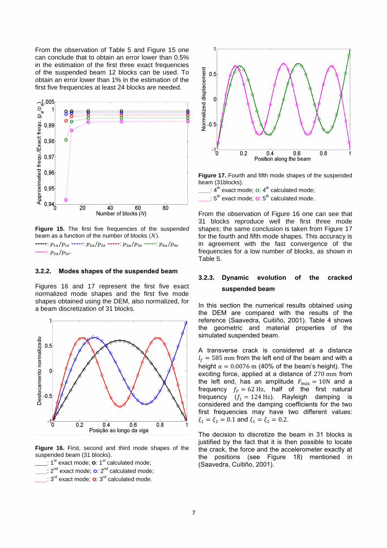
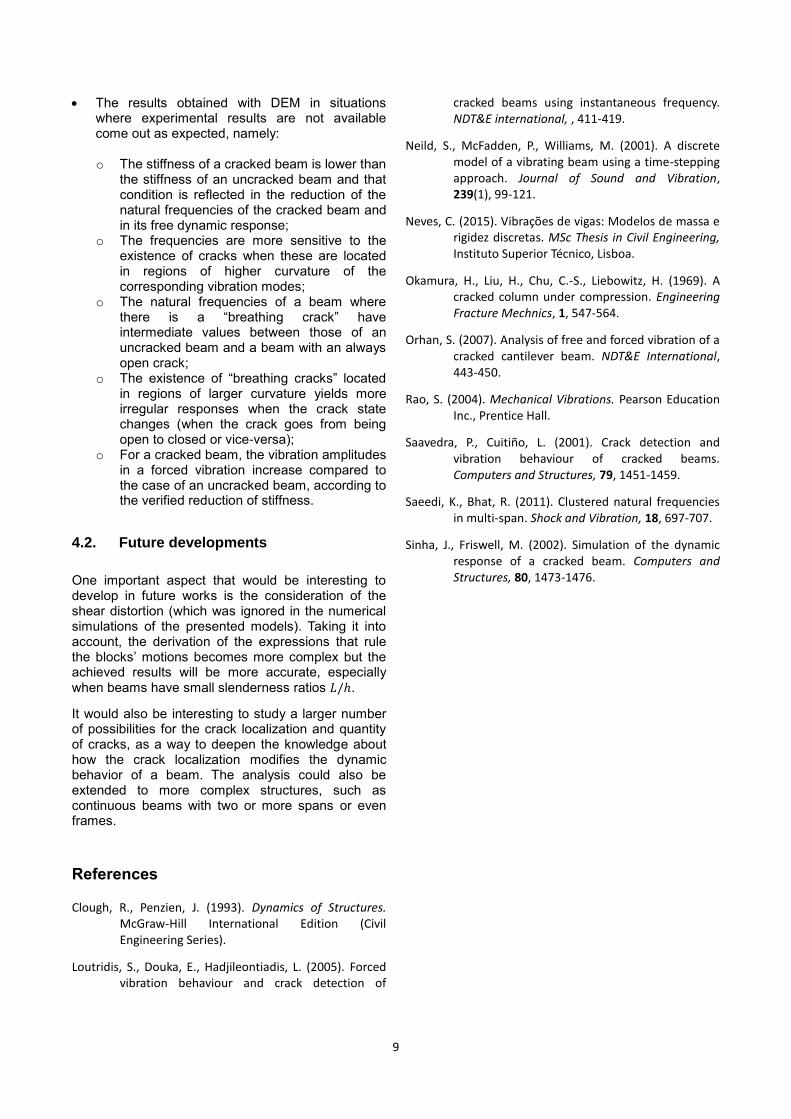
3.2.2. Modes shapes of the suspended beam Figures 16 and 17 represent the first five exact normalized mode shapes and the first five mode shapes obtained using the DEM, also normalized, for a beam discretization of 31 blocks.

Figure 16. First, second and third mode shapes of the

suspended beam (31 blocks).

___: 1st exact mode; o: 1

st calculated mode;

___: 2nd

exact mode; o: 2nd

calculated mode;

___: 3rd

exact mode; o: 3rd

calculated mode.

Figure 17. Fourth and fifth mode shapes of the suspended

beam (31blocks).

___: 4th

exact mode; o: 4th

calculated mode;

___: 5th

exact mode; o: 5th

calculated mode.

From the observation of Figure 16 one can see that 31 blocks reproduce well the first three mode shapes; the same conclusion is taken from Figure 17 for the fourth and fifth mode shapes. This accuracy is in agreement with the fast convergence of the frequencies for a low number of blocks, as shown in Table 5.

3.2.3. Dynamic evolution of the cracked

suspended beam

In this section the numerical results obtained using the DEM are compared with the results of the reference (Saavedra, Cuitiño, 2001). Table 4 shows the geometric and material properties of the simulated suspended beam. A transverse crack is considered at a distance 𝑙𝑓 = 585 mm from the left end of the beam and with a

height 𝑎 = 0.0076 m (40% of the beam’s height). The

exciting force, applied at a distance of 270 mm from the left end, has an amplitude 𝐹máx = 10N and a

frequency 𝑓𝐹 = 62 Hz, half of the first natural

frequency (𝑓1 = 124 Hz). Rayleigh damping is considered and the damping coefficients for the two first frequencies may have two different values: 𝜉1 = 𝜉2 = 0.1 and 𝜉1 = 𝜉2 = 0.2. The decision to discretize the beam in 31 blocks is justified by the fact that it is then possible to locate the crack, the force and the accelerometer exactly at the positions (see Figure 18) mentioned in (Saavedra, Cuitiño, 2001).

8

Figure 18. Crack, force and response evaluation positions.

Figures 19 and 20 represent the acceleration of section A (at a distance of 810 mm from the left end of the beam) calculated with the DEM, considering the existence of a breathing crack, a mesh of 31 blocks and a damping factor 𝜉 = 0.1 or 𝜉 = 0.2 respectively; the results found in the article (Saavedra, Cuitiño, 2001) are also represented in the same Figures.

Figure 19. Acceleration at section A of the suspended

beam (𝜉 = 1%): breathing crack 𝑎 = 0.4ℎ (31 blocks).

____ DEM curve; ▲ Experimental values (Saavedra,

Cuitiño, 2001).

Figure 20. Acceleration at section A of the suspended

beam (𝜉 = 2%): breathing crack 𝑎 = 0.4ℎ (31 blocks).

____ DEM curve; ▲ Experimental values (Saavedra,

Cuitiño, 2001).

One verifies that the approximations obtained with the DEM, especially considering 2% of damping, are quiet acceptable and are, in general, better than the approximations obtained in the models described in the articles (Saavedra, Cuitiño, 2001) and (Sinha & Friswell, 2002).A shift between the response of the model and the experimental response is observed. However, the steady state response from the model has a frequency equal to the frequency of the exciting force. The shift between the responses can be due to the fact that in the experimental situation gravity is present which may produce variations in the crack state.

4. Conclusions

4.1. Contributions

The crack detection in structures is a very important issue and more practical and less onerous detection methods are continuously investigated; this topic is common to many engineering branches such as Civil, Mechanical and Aeronautical. This work intends to contribute to the characterization of the vibrations that the existence of cracks of different characteristics causes in the free or forced dynamic response of some structures. Thus, from the data collected from accelerometers strategically placed in the beam the existence of cracks can be detected and their depth and location may be assessed.

In the course of this work a program in MATLAB environment that allows the application of the Discrete Elements Method (DEM) to the analysis of the dynamic behavior of some structures is developed. Taking as a starting point the model of a simply supported beam, for which expressions were obtained in (Neild et al., 2001), the expressions for the remaining models were derived.

The DEM is a valid and simple method to simulate the behaviour of cracked beams. Based on the presented tables and figures and also on the results presented in (Neves, 2015), the following conclusions could be inferred:

The DEM leads to good approximations of the natural frequencies and mode shapes;

The approximations are better for the lower frequencies and mode shapes, for a given number of blocks used in the discretization, though in some cases the convergence is not monotonous;

The DEM adapts well in the situations where cracks exist and the programation in MATLAB is easily modified;

The results obtained with DEM give good approximations of the experimental results;

9

The results obtained with DEM in situations where experimental results are not available come out as expected, namely:

4.2. Future developments

One important aspect that would be interesting to develop in future works is the consideration of the shear distortion (which was ignored in the numerical simulations of the presented models). Taking it into account, the derivation of the expressions that rule the blocks’ motions becomes more complex but the achieved results will be more accurate, especially when beams have small slenderness ratios 𝐿/ℎ.

It would also be interesting to study a larger number of possibilities for the crack localization and quantity of cracks, as a way to deepen the knowledge about how the crack localization modifies the dynamic behavior of a beam. The analysis could also be extended to more complex structures, such as continuous beams with two or more spans or even frames.

References

Clough, R., Penzien, J. (1993). Dynamics of Structures. McGraw-Hill International Edition (Civil Engineering Series).

Loutridis, S., Douka, E., Hadjileontiadis, L. (2005). Forced vibration behaviour and crack detection of

cracked beams using instantaneous frequency. NDT&E international, , 411-419.

Neild, S., McFadden, P., Williams, M. (2001). A discrete model of a vibrating beam using a time-stepping approach. Journal of Sound and Vibration, 239(1), 99-121.

Neves, C. (2015). Vibrações de vigas: Modelos de massa e rigidez discretas. MSc Thesis in Civil Engineering, Instituto Superior Técnico, Lisboa.

Okamura, H., Liu, H., Chu, C.-S., Liebowitz, H. (1969). A cracked column under compression. Engineering Fracture Mechnics, 1, 547-564.

Orhan, S. (2007). Analysis of free and forced vibration of a cracked cantilever beam. NDT&E International, 443-450.

Rao, S. (2004). Mechanical Vibrations. Pearson Education Inc., Prentice Hall.

Saavedra, P., Cuitiño, L. (2001). Crack detection and vibration behaviour of cracked beams. Computers and Structures, 79, 1451-1459.

Saeedi, K., Bhat, R. (2011). Clustered natural frequencies in multi-span. Shock and Vibration, 18, 697-707.

Sinha, J., Friswell, M. (2002). Simulation of the dynamic response of a cracked beam. Computers and Structures, 80, 1473-1476.

o The stiffness of a cracked beam is lower than the stiffness of an uncracked beam and that condition is reflected in the reduction of the natural frequencies of the cracked beam and in its free dynamic response;

o The frequencies are more sensitive to the existence of cracks when these are located in regions of higher curvature of the corresponding vibration modes;

o The natural frequencies of a beam where there is a “breathing crack” have intermediate values between those of an uncracked beam and a beam with an always open crack;

o The existence of “breathing cracks” located in regions of larger curvature yields more irregular responses when the crack state changes (when the crack goes from being open to closed or vice-versa);

o For a cracked beam, the vibration amplitudes in a forced vibration increase compared to the case of an uncracked beam, according to the verified reduction of stiffness.