bearing fault detection using discrete wavelet

BEARING FAULT DETECTION USING DISCRETE WAVELET TRANSFORM

SYAHRIL AZEEM ONG BIN HAJI MALIKI ONG

Report submitted in partial fulfillment of the requirements

for the award of the degree of Bachelor of Mechanical Engineering

Faculty of Mechanical Engineering

UNIVERSITI MALAYSIA PAHANG

JUNE 2012

vi

ABSTRACT

Rolling element bearing has vast domestic and industrial applications.

Appropriate function of these appliances depends on the smooth operation of the

bearings. Result of various studies shows that bearing problems account for over 40% of

all machine failures. Therefore this research is to design a test rig to harness data in

terms of types of defects and rotation speed and also to develop method to detect

features in vibration signals. Six set of bearings were tested with one of them remains in

good condition while the other five has its own type of defects have been considered for

analysis by using Discrete Wavelet Transform (DWT). The data for a good bearing were

used as benchmark to compare with the defective ones. MATLAB’s Discrete Wavelet

Transform ToolBox was used to down-sample the vibration signals into noticeable form

to detect defect features under certain frequency with respect to time. From the result

generated, Fast Fourier Transform (FFT) and Root Mean Square (RMS) plays an

important role in supporting results analyzed by using DWT from MATLAB® Toolbox.

A system with low operating speed yields unsystematic results due to low excitation. As

the speed increases, the excitation increases thus making DWT works effectively. For

data of insufficient excitation, defect features still may be discovered by calculating and

plotting graph for the percentage of RMS value of each decomposition level compared

to the original input. This shows that DWT appears to be effective in pointing out the

location and frequency of defect when the excitation is high enough. If the excitation is

low, RMS value of each decomposition level may support the result. Nevertheless, DWT

also proves to be an effective method for online condition monitoring tool. Future

research should be detecting defect features by using envelope analysis or based on

statistical tools.

vii

ABSTRAK

Galas mempunyai aplikasi domestik dan industri yang luas. Fungsi yang sesuai

bagi peralatan serta mesin-mesin bergantung kepada kelancaran galas. Hasil daripada

pelbagai kajian menunjukkan bahawa masalah galas merangkumi lebih 40% daripada

kesemua punca kegagalan mesin. Oleh itu, kajian ini adalah untuk mereka bentuk

sebuah rig ujian bagi memperoleh isyarat getaran dari segi jenis kecacatan dan kelajuan

putaran. Kajian ini juga bertujuan untuk membangunkan kaedah untuk mengesan ciri-

ciri di dalam isyarat getaran tersebut. Enam set galas telah diuji dengan salah satu

daripadanya masih dalam keadaan baik manakala lima yang lain mempunyai jenis-jenis

kecacatan yang tertentu dan telah digunakan bagi analisis menggunakan kaedah

Penjelmaan Anak Gelombang Diskrit (DWT). Isyarat getaran yang diperoleh daripada

galas baik telah digunakan sebagai penanda aras untuk dibandingkan dengan isyarat

getaran yang diperoleh dari galas yang tidak sempurna. DWT daripada MATLAB

ToolBox telah digunakan untuk mengurai isyarat-isyarat getaran kepada bentuk yang

lebih ketara bagi mengesan ciri-ciri kecacatan di bawah frekuensi tertentu dengan

merujuk kepada masa. Hasil daripada analisis menunjukkan, Penjelmaan Fourier Pantas

(FFT) dan Punca Min Kuasa Dua (RMS) memainkan peranan penting dalam menyokong

keputusan yang dianalisis dengan menggunakan DWT dari MATLAB ToolBox. Sistem

dengan kelajuan operasi yang rendah menunjukkan keputusan yang tidak sistematik

kesan daripada pengujaan yang rendah. Apabila kelajuan bertambah, peningkatan

pengujaan menyebabkan analisis DWT dapat dilakukan lebih berkesan. Untuk data yang

mempunyai pengujaan yang rendah, ciri-ciri kecacatan masih boleh ditemui melalui

pengiraan dan graf peratusan nilai RMS bagi setiap tahap penguraian berbanding dengan

input asal. Ini menunjukkan bahawa DWT berkesan dalam menunjukkan lokasi dan

kekerapan kecacatan apabila mempunyai pengujaan yang cukup tinggi. Jika pengujaan

rendah, nilai RMS bagi setiap tahap penguraian mampu menyokong keputusan. DWT

juga telah terbukti menjadi kaedah yang berkesan sebagai alat pemantauan keadaan

talian. Kajian akan datang perlu mengesan ciri-ciri kecacatan dengan menggunakan

analisis sampul surat atau berdasarkan alat statistik.

viii

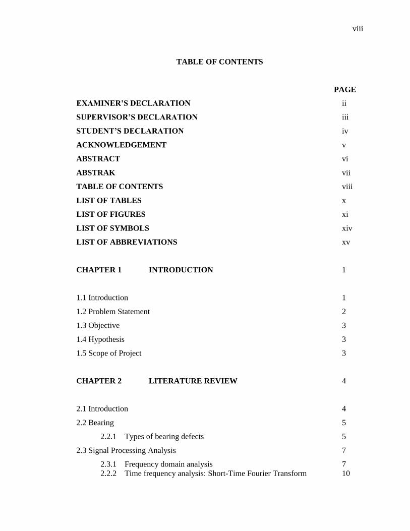
TABLE OF CONTENTS

PAGE

EXAMINER’S DECLARATION ii

SUPERVISOR’S DECLARATION iii

STUDENT’S DECLARATION iv

ACKNOWLEDGEMENT v

ABSTRACT vi

ABSTRAK vii

TABLE OF CONTENTS viii

LIST OF TABLES x

LIST OF FIGURES xi

LIST OF SYMBOLS xiv

LIST OF ABBREVIATIONS xv

CHAPTER 1 INTRODUCTION 1

1.1 Introduction 1

1.2 Problem Statement 2

1.3 Objective 3

1.4 Hypothesis 3

1.5 Scope of Project 3

CHAPTER 2 LITERATURE REVIEW 4

2.1 Introduction 4

2.2 Bearing 5

2.2.1 Types of bearing defects 5

2.3 Signal Processing Analysis 7

2.3.1 Frequency domain analysis 7

2.2.2 Time frequency analysis: Short-Time Fourier Transform 10

ix

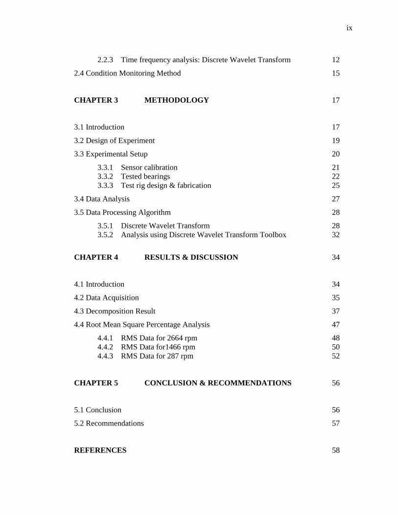
2.2.3 Time frequency analysis: Discrete Wavelet Transform 12

2.4 Condition Monitoring Method 15

CHAPTER 3 METHODOLOGY 17

3.1 Introduction 17

3.2 Design of Experiment 19

3.3 Experimental Setup 20

3.3.1 Sensor calibration 21

3.3.2 Tested bearings 22

3.3.3 Test rig design & fabrication 25

3.4 Data Analysis 27

3.5 Data Processing Algorithm 28

3.5.1 Discrete Wavelet Transform 28

3.5.2 Analysis using Discrete Wavelet Transform Toolbox 32

CHAPTER 4 RESULTS & DISCUSSION 34

4.1 Introduction 34

4.2 Data Acquisition 35

4.3 Decomposition Result 37

4.4 Root Mean Square Percentage Analysis 47

4.4.1 RMS Data for 2664 rpm 48

4.4.2 RMS Data for1466 rpm 50

4.4.3 RMS Data for 287 rpm 52

CHAPTER 5 CONCLUSION & RECOMMENDATIONS 56

5.1 Conclusion 56

5.2 Recommendations 57

REFERENCES 58

x

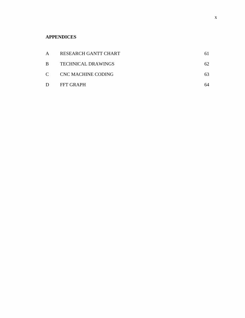
APPENDICES

A RESEARCH GANTT CHART 61

B TECHNICAL DRAWINGS 62

C CNC MACHINE CODING 63

D FFT GRAPH 64

xi

LIST OF TABLES

Table No Page

2.1 Types of bearing damage, appearance, and possible cause 6

2.2 Fault description in the ball bearings 16

3.1 Number of experiment run with various bearing defects 19

3.2 Types and location of defect 22

4.1 RMS percentage value for each level of decomposition 48

at 2664 rpm


at1466 rpm


at 287 rpm

xii

LIST OF FIGURES

Figure No Page

2.1 Cutaway view of a caged ball bearing 5

2.2 A typical spectrum obtained from a rolling element bearing 9

with an inner race defect

2.3 STFT in displacement (a), velocity (b), and acceleration (c) 11

of a good bearing. The colour associates to the higher value

of the energy scale, and represents a high level of energy content

2.4 STFT in displacement (a), velocity (b), and acceleration (c) 12

of a faulty bearing. The colour associates to the higher value

of the energy scale, and represents a high level of energy content

2.5 Comparison of known transformation methods. Time-series 14

(a), Fourier transform (b), STFT (c), and Wavelet transform (d)

3.1 Project’s flow chart 18

3.2 Bearing fault detection test rig consist of: coupling (a), tested 20

bearing (b), flywheel (c), healthy bearing (d), accelerometer (e),

data acquisition system (f), and a PC with DASYlab software (g)

3.3 Actual bearing test rig 21

3.4 Outer race defect 22

3.5 Inner race defect 23

3.6 Contaminated defect 23

3.7 Point defect 24

3.8 Corroded defect 24

3.9 Healthy bearing 25

3.10 Bearing housing’s isometric view 26

3.11 Fly wheel’s isometric view 26

xiii

3.12 Shaft’s front view 27

3.13 DASYLab’s layout 27

3.14 Flow chart for decomposition process by using MATLAB®’s 29

command

3.15 Filtering process at its most basic level 30

3.16 Down-sampling process from left to right 30

3.17 Wavelet decomposition tree 31

3.18 Discrete Wavelet Transform’s Toolbox main menu 32

3.19 Selecting data (a), choosing wavelet type (b), and changing 33

display mode (c)

3.20 Output for MATLAB Discrete Wavelet Transform’s Toolbox 33

4.1 Vibration reading when running at 287 rpm for healthy 35

bearing (a), PD (b), OR defect (c), IR defect (d), CN

defect (e), and CB defect (f)







4.4 Decomposition result for healthy bearing at 287 rpm 38



4.7 Decomposition result for outer race defect at 287 rpm 40



4.10 Decomposition result for inner race defect 287 rpm 41

xiv



4.13 Decomposition result for corroded defect at 287 rpm 43



4.16 Decomposition result for point defect at 287 rpm 44



4.19 Decomposition result for contaminated defect at 287 rpm 46



4.22 RMS percentage vs. decomposition level for speed of 2664 rpm 49



4.25 FFT result for contaminated defect at speed 297 rpm 55

xv

LIST OF SYMBOLS

- Shaft rotation frequency

α - Contact angle

Han(h) - Hanning function

V(tn) - nth measured voltage sample

Ψ(t) - Mother wavelet

xvi

LIST OF ABBREVIATIONS

AE - Acoustic Emission

BG - Burnt grease

B&K - Bruel & Kjær

cA - Approximate decomposition

CB - Corroded ball

cD - Detailed decomposition

CWT - Continuous Wavelet Transform

DWT - Discrete Wavelet Transform

FFT - Fast Fourier Transform

HDD - Hard disk drive

HFRT - High frequency resonance technique

IR - Inner race

NDT - Non-destructive test

NiDAQ - National Instrument Data Acquisition System

OR - Outer race

PC - Personal computer

PD - Point defect

RMS - Root Mean Square

RPM - Revolutions per minute

SPM - Shock Pulse Method

STFT - Short Time Fourier Transform

UI - User interface

CHAPTER 1

INTRODUCTION

1.1 INTRODUCTION

Rolling element bearings has vast domestic and industrial applications.

Appropriate function of these appliances depends on the smooth operation of the

bearings. In industrial applications, bearings are considered as critical mechanical

components and a defect in such a bearing causes malfunction and may even lead to

catastrophic failure of the machinery.

Presently, vibration monitoring method becomes the most reliable tool as a part

of preventive maintenance for rotating machines (Tandon and Choudhury, 1999). The

vibration data often contain fault signatures where several signal processing techniques;

often adapted to a precise defect type, results to online monitoring system.

There are many condition monitoring methods used for detection and diagnosis

of rolling element bearing defects such as vibration measurements, temperature

measurement, shock pulse method (SPM), and acoustic emission (AE). Various

researchers suggested that stator current monitoring can provide the same indications

without requiring access to the motor. This technique utilizes results of spectral analysis

of the stator current or supply current of any part nearest to the rolling bearing element

for diagnosis purpose (Schoen et al, 1995). Other signal processing technique for

condition monitoring method includes averaging technique (Braun and Datner, 1977),

adaptive noise cancelling (Chaturvedi and Thomas, 1981), and high-frequency

2

resonance technique (HFRT) (Prasad et al, 1984) was developed to improve signal-to-

noise ratio for more effective detection of bearing defect. Among all these monitoring

methods, the high-frequency resonance technique is more popular for bearing fault

detection. However, most of the method requires additional computations and several

runs of impact tests to find the bearing resonance frequency. Therefore, extra

instruments such as vibration exciters and their controller are needed for HFRT

(Prabhakar et al, 2002).

Discrete Wavelet Transform (DWT) on the other hand, were proven to be the

best condition monitoring method/effective tool for detecting single and multiple faults

in the ball bearings (Djebala et al, 2007; Prabhakar et al, 2002). A clear review on using

DWT as condition monitoring method and possible early detection was given by Tandon

and Choudhury (1999), Kim et al. (2002), and Staszewski (1998).

1.2 PROBLEM STATEMENT

Rolling bearings are the major components of rotating machine. Thus they are

often subjected to various excitations which can cause dangerous accidents due to

certain factors. Results of various studies show that bearing problems account for over

40% of all machine failure (Schoen 1995).

This data acquisition technique is a type of non destructive test (NDT) which

doesn’t require the user to dismantle the bearing from the machine in order to check its

condition as it may be presented through online monitoring.

Time-domain analysis lacks information in terms of frequency while frequency-

domain analysis lacks information on time. Even though Short Time Fourier Transform

(STFT) have both time and frequency domain analysis, but it is less accurate on both

domain of analysis. But DWT on the other hand, produces vibratory signal in terms of

time and frequency domain analysis which gives the most accurate readings for caged-

roller bearing which is why DWT was chosen as the tool to analyze bearing defects.

3

1.3 OBJECTIVE

The objective of this project is:

a) Design a test rig to harness vibration data in terms of types of defects and

rotation speed

b) Develop method to detect the defect features in the vibration signals by

using time-frequency domain analysis

1.4 HYPOTHESIS

The expected result for this research is that there will be a difference in terms of

vibration signals when bearing with different type of defects were tested by using

wavelet transform method. DWT method is an advanced method to detect any changes

in terms of vibration signal.

1.5 SCOPE OF PROJECT

In order to reach the project’s objective, the following scopes are identified:

a) Only horizontal deep groove ball bearings will be used

b) Five types of bearing defects will be tested and they are outer race (OR)

defect, inner race (IR) defect, point defect (PD), corroded ball (CB)

defects, contaminated defect (CN), and a good condition bearing as the

reference

c) Three different angular speed of lowest, medium, and highest speed will

be used to acquire data for each bearings

d) Acquire vibration data from the rotating machine using a single axial

accelerometer

e) Analysis will be done by using MATLAB®’s Discrete Wavelet

Transform ToolBox

4

CHAPTER 2

LITERATURE REVIEW

2.1 INTRODUCTION

This chapter discusses the literatures that are related to bearing fault detection

and discrete wavelet transform. In this chapter, the types of bearings, types of bearing

defects, and common causes of bearing failures will be discussed. Moreover, the signal

processing analysis on different types of domain analysis, and condition monitoring

methods also on different types of domain analysis will also discussed.

5

2.2 BEARING

Bearing; as shown in Figure 2.1, is a mechanical device that allows constrained

relative motion of 2 or more parts; typically between linear and rotational movement.

There are many types of bearings often used in machineries when it involves rolling

element and each one of them used for different purpose. These include ball bearings,

caged ball bearings, roll thrust bearings, and tapered roller thrust bearings.

Figure 2.1: Cutaway view of a caged ball bearing

Source: The Timken Company. (2011)

2.2.1 Types of bearing defects

As well as there’s continuous usage there will always be unwanted defects on the

material of the bearing. Generally, a rolling bearing cannot rotate forever. Under normal

operating conditions of balanced load and good alignment, fatigue failure begins with a

small fissure, located between the surface of the raceway and the rolling elements, which

gradually propagate to the surface, generating detectable vibrations and increasing noise

levels (Eschmann et al 1958). Continued stress causes fragments of the material to break

loose producing a localized fatigue phenomenon known as flaking or spalling (Riddle

1955). The affected area expands rapidly afterwards contaminating the lubrication and

6

causing localized overloading over the entire circumference of the raceway (Eschmann

et al 1958). Eventually, the failure results in rough running of the bearing

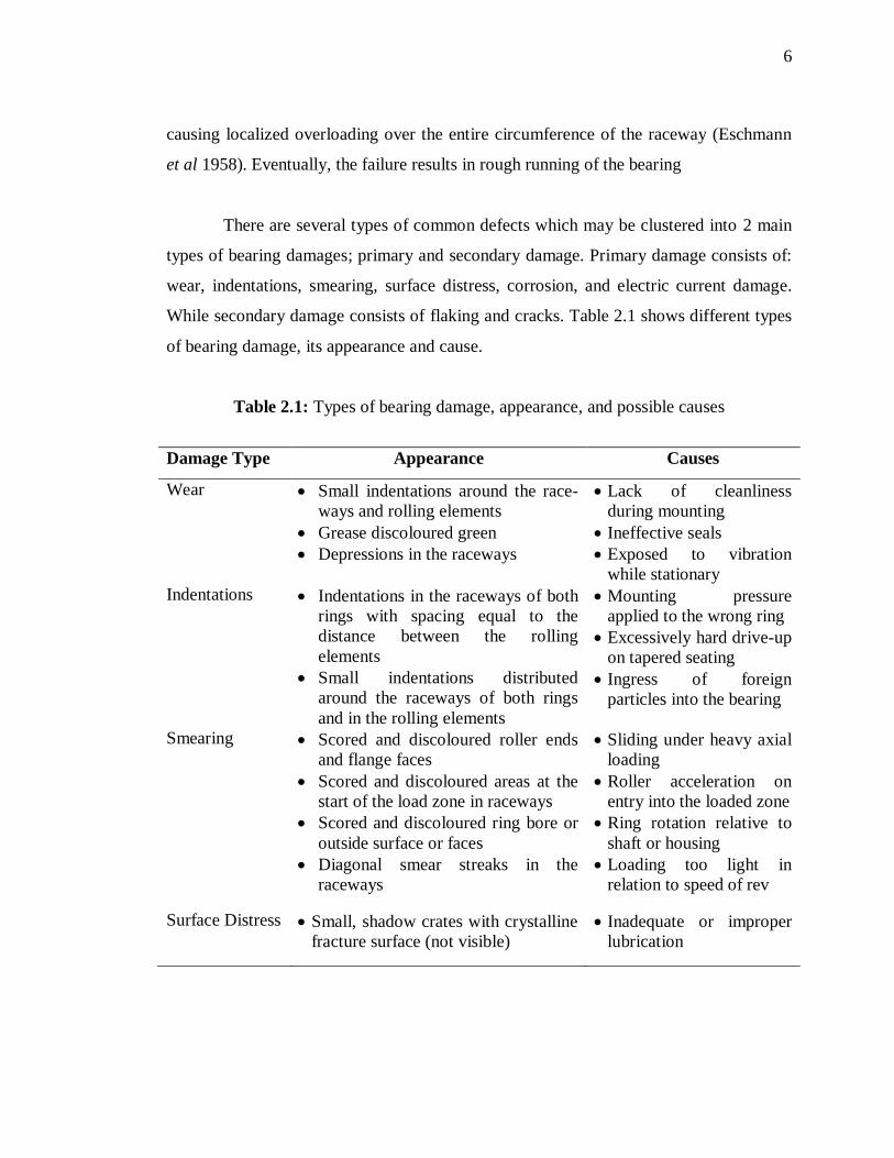
There are several types of common defects which may be clustered into 2 main

types of bearing damages; primary and secondary damage. Primary damage consists of:

wear, indentations, smearing, surface distress, corrosion, and electric current damage.

While secondary damage consists of flaking and cracks. Table 2.1 shows different types

of bearing damage, its appearance and cause.

Table 2.1: Types of bearing damage, appearance, and possible causes

Damage Type Appearance Causes

Wear Small indentations around the race-

ways and rolling elements

Grease discoloured green

Depressions in the raceways

Lack of cleanliness

during mounting

Ineffective seals

Exposed to vibration

while stationary

Indentations Indentations in the raceways of both

rings with spacing equal to the

distance between the rolling

elements

Small indentations distributed

around the raceways of both rings

and in the rolling elements

Mounting pressure

applied to the wrong ring

Excessively hard drive-up

on tapered seating

Ingress of foreign

particles into the bearing

Smearing

Scored and discoloured roller ends

and flange faces

Scored and discoloured areas at the

start of the load zone in raceways

Scored and discoloured ring bore or

outside surface or faces

Diagonal smear streaks in the

raceways

Sliding under heavy axial

loading

Roller acceleration on

entry into the loaded zone

Ring rotation relative to

shaft or housing

Loading too light in

relation to speed of rev

Surface Distress Small, shadow crates with crystalline

fracture surface (not visible)

Inadequate or improper

lubrication

7

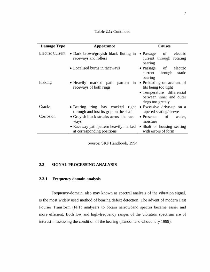
Table 2.1: Continued

Damage Type Appearance Causes

Electric Current Dark brown/greyish black fluting in

raceways and rollers

Localised burns in raceways

Passage of electric

current through rotating

bearing

Passage of electric

current through static

bearing

Flaking Heavily marked path pattern in

raceways of both rings

Preloading on account of

fits being too tight

Temperature differential

between inner and outer

rings too greatly

Cracks Bearing ring has cracked right

through and lost its grip on the shaft

Excessive drive-up on a

tapered seating/sleeve

Corrosion Greyish black streaks across the race-

ways

Raceway path pattern heavily marked

at corresponding positions

Presence of water,

moisture

Shaft or housing seating

with errors of form

Source: SKF Handbook, 1994

2.3 SIGNAL PROCESSING ANALYSIS

2.3.1 Frequency domain analysis

Frequency-domain, also may known as spectral analysis of the vibration signal,

is the most widely used method of bearing defect detection. The advent of modern Fast

Fourier Transform (FFT) analysers to obtain narrowband spectra became easier and

more efficient. Both low and high-frequency ranges of the vibration spectrum are of

interest in assessing the condition of the bearing (Tandon and Choudhury 1999).

8

When an interaction of defect occurs in rolling element bearings, it produces

pulses of very short duration. There will be an increase in the vibrational energy during

high frequency due to the pulses excites the natural frequencies of bearing elements or

the nearby structures. The resonant frequencies may be calculated theoretically as

proved by (Tandon and Nakra, 1992).

Each bearing elements has their own characteristic rotational frequency. There’s

an increase in vibrational energy at the element’s rotational frequency whenever there’s

a defect on a particular bearing. These characteristic defect frequencies can be calculated

from kinematic considerations. For a bearing with a stationary outer race, these

frequencies are given by the following expressions:

Cage frequency , proposed by Mathew and Alfredson (1984):

Ball spinning frequency , proposed by McFadden and Smith (1984a):

Outer race defect frequency , proposed by Kim (1984a):

Inner race defect frequency , also proposed by Kim (1984b):

and

Rolling element defect frequency , proposed by Sunnersjo (1978):

(2.1)

(2.2)

(2.3)

(2.4)

(2.5)

9

where,

is the shaft rotation frequency in rad/s

d is the diameter of the rolling element

D is the pitch diameter

Z is the number of rolling elements, and

α is the contact angle.

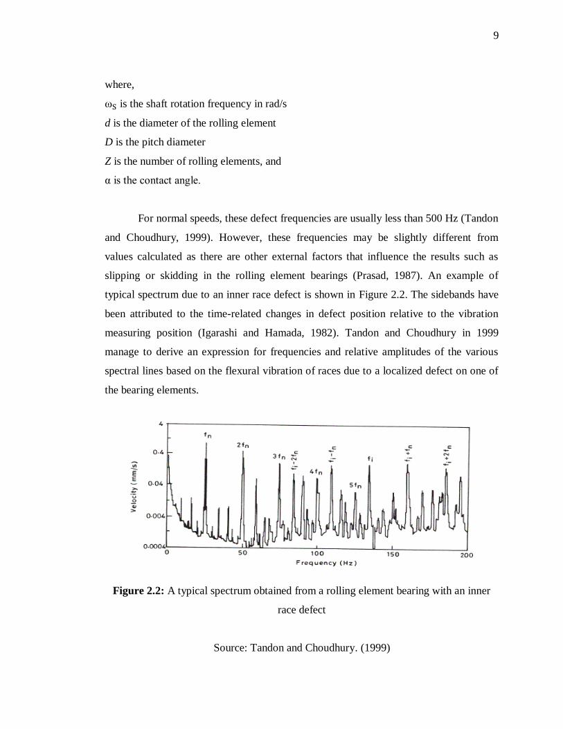
For normal speeds, these defect frequencies are usually less than 500 Hz (Tandon

and Choudhury, 1999). However, these frequencies may be slightly different from

values calculated as there are other external factors that influence the results such as

slipping or skidding in the rolling element bearings (Prasad, 1987). An example of

typical spectrum due to an inner race defect is shown in Figure 2.2. The sidebands have

been attributed to the time-related changes in defect position relative to the vibration

measuring position (Igarashi and Hamada, 1982). Tandon and Choudhury in 1999

manage to derive an expression for frequencies and relative amplitudes of the various

spectral lines based on the flexural vibration of races due to a localized defect on one of

the bearing elements.

Figure 2.2: A typical spectrum obtained from a rolling element bearing with an inner

race defect

Source: Tandon and Choudhury. (1999)

10

(2.6)

2.3.2 Time-frequency analysis: Short Time Fourier Transform

One of the shortcomings of the Fourier Transform is that it doesn’t give

information on time at which a frequency component occurs. It will be a major problem

to non-stationary signals compared to stationary signals. Therefore, one approach which

can give information on the time resolution of the spectrum is the Short Time Fourier

Transform (STFT). The STFT as proposed by Lyon (1984) is defined as:

where L represents the length of one block of data, tn is the time instant of STFT and

V(tn) is the nth measured voltage sample. The term Han(h) represents the Hanning

function chosen as the analysis window.

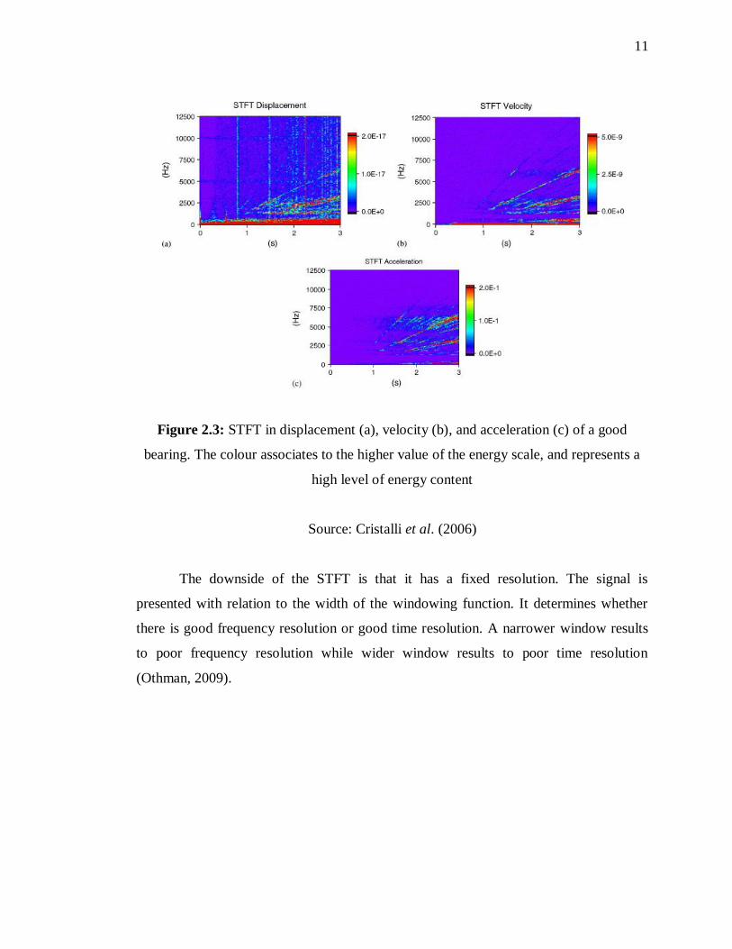
Figure 2.3 and Figure 2.4 represents the STFT computed for a good and a faulty

bearing. The displacement measurements by laser vibrometer reveal vertical lines caused

by a single dropout, which add impulse noise to the signal. The disturbances have not

appeared in any of the measurements of velocity and acceleration.

11

Figure 2.3: STFT in displacement (a), velocity (b), and acceleration (c) of a good

bearing. The colour associates to the higher value of the energy scale, and represents a

high level of energy content

Source: Cristalli et al. (2006)

The downside of the STFT is that it has a fixed resolution. The signal is

presented with relation to the width of the windowing function. It determines whether

there is good frequency resolution or good time resolution. A narrower window results

to poor frequency resolution while wider window results to poor time resolution

(Othman, 2009).

12

(2.7)

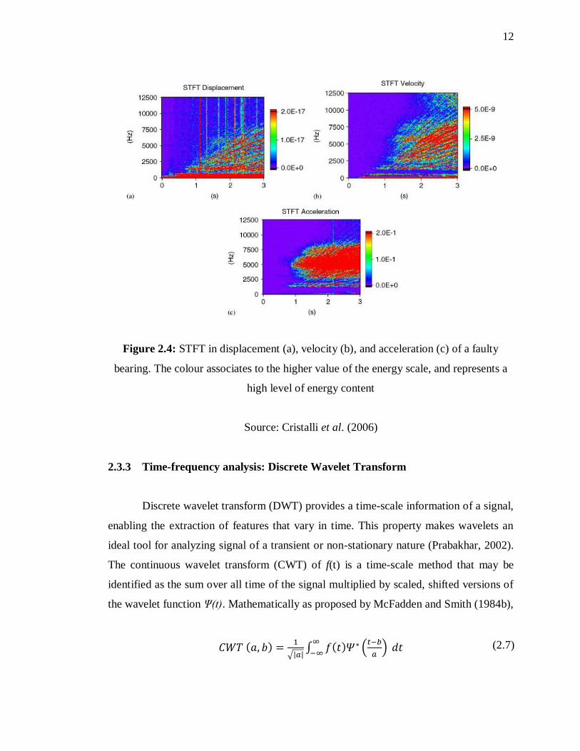
Figure 2.4: STFT in displacement (a), velocity (b), and acceleration (c) of a faulty

bearing. The colour associates to the higher value of the energy scale, and represents a

high level of energy content

Source: Cristalli et al. (2006)

2.3.3 Time-frequency analysis: Discrete Wavelet Transform

Discrete wavelet transform (DWT) provides a time-scale information of a signal,

enabling the extraction of features that vary in time. This property makes wavelets an

ideal tool for analyzing signal of a transient or non-stationary nature (Prabakhar, 2002).

The continuous wavelet transform (CWT) of f(t) is a time-scale method that may be

identified as the sum over all time of the signal multiplied by scaled, shifted versions of

the wavelet function Ψ(t). Mathematically as proposed by McFadden and Smith (1984b),

bearing fault detection using discrete wavelet

Documents