BeBoP: A Cost Effective Predictor Infrastructure for

Superscalar Value Prediction

Arthur Perais, Andre Seznec

To cite this version:

Arthur Perais, Andre Seznec. BeBoP: A Cost Effective Predictor Infrastructure for Super-scalar Value Prediction. International Symposium on High Performance Computer Architec-ture, Feb 2015, San Francisco, United States. 21, pp.13 - 25 ), <http://darksilicon.org/hpca/>.<10.1109/HPCA.2015.7056018>. <hal-01193175>

HAL Id: hal-01193175

https://hal.inria.fr/hal-01193175

Submitted on 4 Sep 2015

HAL is a multi-disciplinary open accessarchive for the deposit and dissemination of sci-entific research documents, whether they are pub-lished or not. The documents may come fromteaching and research institutions in France orabroad, or from public or private research centers.

L’archive ouverte pluridisciplinaire HAL, estdestinee au depot et a la diffusion de documentsscientifiques de niveau recherche, publies ou non,emanant des etablissements d’enseignement et derecherche francais ou etrangers, des laboratoirespublics ou prives.

BeBoP: A Cost Effective Predictor Infrastructure forSuperscalar Value Prediction

Arthur Perais Andre SeznecIRISA/INRIA

Campus de Beaulieu35042 Rennes, France

{arthur.perais,Andre.Seznec}@inria.fr

Abstract—Up to recently, it was considered that aperformance-effective implementation of Value Prediction (VP)would add tremendous complexity and power consumption in thepipeline, especially in the Out-of-Order engine and the predictorinfrastructure.

Despite recent progress in the field of Value Prediction, thisremains partially true. Indeed, if the recent EOLE architectureproposition suggests that the OoO engine need not be alteredto accommodate VP, complexity in the predictor infrastructureitself is still problematic. First, multiple predictions must begenerated each cycle, but multi-ported structures should beavoided. Second, the predictor should be small enough to beconsidered for implementation, yet coverage must remain highenough to increase performance.

To address these remaining concerns, we first proposea block-based value prediction scheme mimicking currentinstruction fetch mechanisms, BeBoP. It associates the predictedvalues with a fetch block rather than distinct instructions.Second, to remedy the storage issue, we present the DifferentialVTAGE predictor. This new tightly coupled hybrid predictorcovers instructions predictable by both VTAGE and Stride-basedvalue predictors, and its hardware cost and complexity can bemade similar to those of a modern branch predictor. Third, weshow that block-based value prediction allows to implement thecheckpointing mechanism needed to provide D-VTAGE with lastcomputed/predicted values at moderate cost.

Overall, we establish that EOLE with a 32.8KB block-basedD-VTAGE predictor and a 4-issue OoO engine can significantlyoutperform a baseline 6-issue superscalar processor, by up to62.2% and 11.2% on average (gmean), on our benchmark set.

I. INTRODUCTION & MOTIVATIONS

Single thread performance is still an issue ingeneral-purpose computing. In that context, architecturaltechniques that were proposed in the late 90’s for high-enduniprocessors but were not implemented at that time could beworth revisiting; among these techniques is Value Prediction(VP), that was independently proposed by Gabbay et al. [22]and Lipasti et al. [20].

Value Prediction suffers from an asymmetry betweenthe small average performance gains brought by a correctprediction and the high cost of recovering from amisprediction. This implies that to increase performance, VPmust be very accurate, and/or the recovery mechanism mustbe very aggressive, e.g. selective replay. As a result, it wasconsidered up to recently that VP would lead to a huge increase

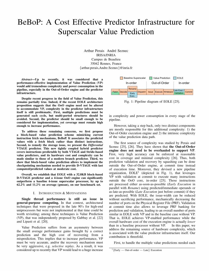
Fig. 1: Pipeline diagram of EOLE [25].

in complexity and power consumption in every stage of thepipeline.

However, taking a step back, only two distinct componentsare mostly responsible for this additional complexity: 1) theOut-of-Order execution engine and 2) the intrinsic complexityof the value prediction data path.

The first source of complexity was studied by Perais andSeznec [25], [26]. They have shown that the Out-of-Orderengine does not need to be overhauled to support VP.First, very high accuracy can be enforced at reasonablecost in coverage and minimal complexity [26]. Thus, bothprediction validation and recovery by squashing can be doneoutside the Out-of-Order engine, at commit time insteadof execution time. Moreover, they devised a new pipelineorganization, EOLE1 (depicted in Fig. 1), that leveragesVP with validation at commit to execute many instructionsoutside the OoO core, in-order [25]. Those instructionsare processed either as-soon-as-possible (Early Execution inparallel with Rename) using predicted/immediate operands oras-late-as-possible (Late Execution just before commit) if theyare predicted. With EOLE, the issue-width can be reducedwithout sacrificing performance, mechanically decreasing thenumber of ports on the Physical Register File (PRF). Validationat commit time also allows to leverage PRF banking forprediction and validation, leading to an overall number of portssimilar in EOLE with VP and in the baseline case without VP.That is, EOLE achieves VP-enabled performance while theoverall hardware cost of the execution engine is actually lowerthan in a baseline processor without VP. In this paper, weaddress the remaining source of hardware complexity, whichis associated with the value predictor infrastructure itself. Ourcontribution is threefold.

First, to handle the multiple value predictions needed each

1{Early — Out-of-order — Late} Execution

cycle in a wide issue processor, we propose Block-Basedvalue Prediction (BBP or BeBoP). With this scheme, allthe predictions associated with an instruction fetch block areput in a single predictor entry. The predictor is thereforeaccessed with the PC of the instruction fetch block andthe whole group of predictions is retrieved in a singleread. BeBoP accommodates currently implemented instructionfetch mechanisms. However, it only addresses complexity ofoperation, but not storage requirement.

As a result, in a second step, we propose a space-efficienthybrid predictor, D-VTAGE, by tightly coupling VTAGE[26] and a Stride-based predictor [7]. D-VTAGE is veryspace-efficient as it can use partial strides (e.g. 8- and 16-bit).Its storage cost can be made equivalent to that of the I-Cacheor the branch predictor.

Third, we devise a cost-effective checkpoint-basedimplementation of the speculative last-value window. Sucha window is required due to the presence of a Stride-basedprediction scheme in D-VTAGE. Without it, instructions inloops that can fit several times inside the instruction windoware unlikely to be correctly predicted.

The remainder of this paper is organized as follows: SectionII describes the issues related to predicting several valuesper cycle and introduces BeBoP. Section III introduces theD-VTAGE predictor and the way it operates while Section IVdiscusses practical mechanisms to implement D-VTAGE onactual silicon. Section V reviews our evaluation framework.Section VI details the results of our experiments and givesinsights on the impact of some predictor parameters onperformance. Section VII describes related work. Finally,Section VIII provides concluding remarks.

II. BLOCK-BASED VALUE PREDICTION

A. Issues on Concurrent Multiple Value Predictions

Modern superscalar processors are able to fetch/decodeseveral instructions per cycle. Ideally, the value predictorshould be able to predict a value for all possible outcomesof all instructions fetched during that cycle.

For predictors that do not use any local value history toread tables (e.g. the Last Value Predictor, the Stride predictoror VTAGE), and when using a RISC ISA producing atmost one result per instruction (e.g. Alpha), a straightforwardimplementation of the value predictor consists in mimickingthe organization of the instruction fetch hardware in thedifferent components of predictor. Predictions for contiguousinstructions are stored in contiguous locations in the predictorcomponents and the same interleaving structures are usedin the instruction cache, the branch predictor and the valuepredictor. However, for predictors using local value history(e.g. FCM [32]), even in this very favorable scenario,the predictor components must be bank-interleaved at theinstruction level and the banks individually accessed withdifferent indexes.

Moreover, the most popular ISAs do not have the regularityproperty of Alpha. For x86 – that we consider in this study –some instructions may produce several results, and informationsuch as the effective PC of instructions in the block2 and the

2Storing boundary bits in the I-cache can remedy this, but at high cost [1].

number of produced values are known after several cycles(after pre-decoding and after Decode, respectively). That is,there is no natural way to associate a value predictor entrywith a precise PC: Smooth multiple-value prediction on avariable-length ISA remains a challenge in itself.

B. Block-based Value-Predictor accesses

We remedy this fundamental issue by proposingBlock-Based value Prediction (BeBoP). To introduce thisnew access scheme and layout, we consider a VTAGE-likepredictor, but note that block-based prediction can begeneralized to any predictor.

The idea is to access the predictor using the fetch-block PC(i.e. the current PC right-shifted by log2(fetchBlockSize)),as well as some extra global information as defined in VTAGE[26]. Instead of containing a single value, the entry that isaccessed now consists in Npred values (Npred > 0). The mth

value in the predictor entry is associated with the mth resultin the fetch block, and not with its precise PC.

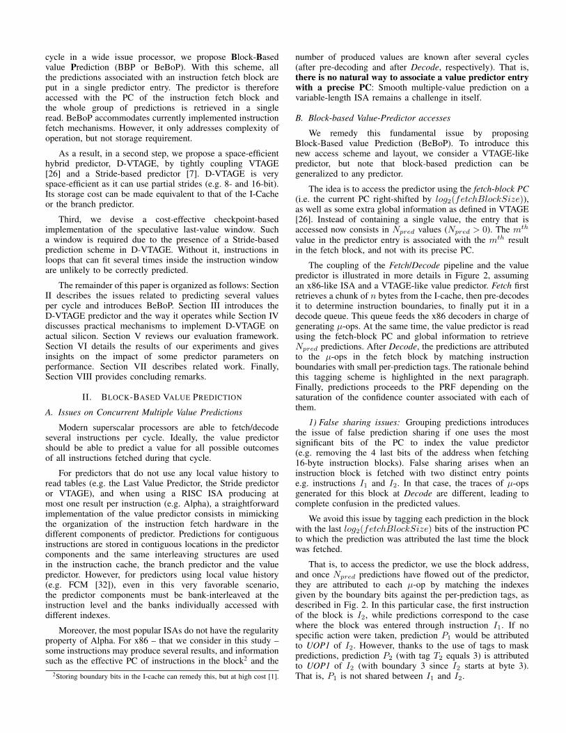
The coupling of the Fetch/Decode pipeline and the valuepredictor is illustrated in more details in Figure 2, assumingan x86-like ISA and a VTAGE-like value predictor. Fetch firstretrieves a chunk of n bytes from the I-cache, then pre-decodesit to determine instruction boundaries, to finally put it in adecode queue. This queue feeds the x86 decoders in charge ofgenerating µ-ops. At the same time, the value predictor is readusing the fetch-block PC and global information to retrieveNpred predictions. After Decode, the predictions are attributedto the µ-ops in the fetch block by matching instructionboundaries with small per-prediction tags. The rationale behindthis tagging scheme is highlighted in the next paragraph.Finally, predictions proceeds to the PRF depending on thesaturation of the confidence counter associated with each ofthem.

1) False sharing issues: Grouping predictions introducesthe issue of false prediction sharing if one uses the mostsignificant bits of the PC to index the value predictor(e.g. removing the 4 last bits of the address when fetching16-byte instruction blocks). False sharing arises when aninstruction block is fetched with two distinct entry pointse.g. instructions I1 and I2. In that case, the traces of µ-opsgenerated for this block at Decode are different, leading tocomplete confusion in the predicted values.

We avoid this issue by tagging each prediction in the blockwith the last log2(fetchBlockSize) bits of the instruction PCto which the prediction was attributed the last time the blockwas fetched.

That is, to access the predictor, we use the block address,and once Npred predictions have flowed out of the predictor,they are attributed to each µ-op by matching the indexesgiven by the boundary bits against the per-prediction tags, asdescribed in Fig. 2. In this particular case, the first instructionof the block is I2, while predictions correspond to the casewhere the block was entered through instruction I1. If nospecific action were taken, prediction P1 would be attributedto UOP1 of I2. However, thanks to the use of tags to maskpredictions, prediction P2 (with tag T2 equals 3) is attributedto UOP1 of I2 (with boundary 3 since I2 starts at byte 3).That is, P1 is not shared between I1 and I2.

Fig. 2: Prediction attribution with BeBoP and 8-byte fetch blocks. The predictor is accessed with the currently fetched PC andpredictions are attributed using byte indexes as tags.

Tags are modified when the predictor is updated withthe following constraint: a greater tag never replaces alesser tag, so that the entry can learn the ”real” location ofinstructions/µ-ops in the block. For instance, if the block wasentered through I2 but has already been entered through I1before, then the tag associated with P1 is the address of thefirst byte of I1 (i.e. 0). The address of the first byte of I2 isgreater than that of I1, so it will not replace the tag associatedwith P1 in the predictor, even though dynamically, for thatinstance of the block, I2 is the first instruction of the block. Asa result, the pairing P1/I1 is preserved throughout execution.This constraint does not apply when the entry is allocated.

2) On the Number of Predictions in Each Entry: Thenumber of µ-ops producing a register depends on theinstructions in the block, but only the size of the instructionfetch block is known at design-time. Thus, Npred should bechosen as a tradeoff between coverage (i.e. provision enoughpredictions in an entry for the whole fetch block) and wastedarea (i.e. having too many predictions provisioned in the entry).For instance, in Figure 2, since I1 and I2 both consume aprediction, only UOP2 of instruction I3 can be predicted.

In Section VI-B, we will study the impact of varying Npred

while keeping the size of the predictor constant. Specifically,a too small Npred means that potential is lost while a too bigNpred means that space is wasted as not all prediction slots inthe predictor entry are used. Additionally, at constant predictorsize, a smaller Npred means more entries, hence less aliasing.

3) Free Load Immediate Prediction: Our implementationof Value Prediction features write ports available at dispatchtime to write predictions to the PRF. Thus, it is not necessaryto predict load immediate instructions3 since their actual resultis available in the front-end. The predictor need not be trainedfor these instructions, and they need not be validated or evendispatched to the IQ. They can be processed in the front-endeven without the Early Execution stage of EOLE [25], by

3With the exception of load immediate instructions that write to a partialregister.

simply placing the decoded immediate in the PRF. Due to thisoptimization, the addition of a specific table that would onlypredict small constants [31] may become much less interesting.

4) Multiple Blocks per Cycle: In order to provide highinstruction fetch bandwidth, several instruction blocks arefetched in parallel on wide-issue processors. For instance, onthe EV8 [35], two instruction fetch blocks are retrieved eachcycle. To support this parallel fetch, the instruction cache hasto be either fully dual-ported or bank-interleaved. In the lattercase, a single block is fetched on a conflict unless the sameblock appears twice. Since fully dual-porting is much morearea- and power-consuming, bank interleaving is generallypreferred.

In BeBoP, the (potential) number of accesses per cycle tothe predictor tables is similar to the number of accesses madeto the branch predictor tables, i.e. up to 3 accesses per fetchblock: Read at fetch time, second read at commit time andwrite to update. This adds up to 6 accesses per cycle if twoinstruction blocks are fetched each cycle.

However, for value predictor or branch predictorcomponents that are indexed using only the block PC (e.g. LastValue component of VTAGE and Stride predictors), one canreplicate the same bank interleaving as the instruction cache inthe general case. If the same block is accessed twice in a singlecycle, Stride-based predictors must provision specific hardwareto compute predictions for both blocks. This can be handledthrough computing both (Last Value + stride) and (Last Value+ stride1 + stride2) using 3-input adders.

For value or branch predictor components that are indexedusing the global branch history or the path history, such asVTAGE tagged components, one can rely on the interleavingscheme that was proposed to implement the branch predictorin the EV8 [35]. By forcing consecutive accesses to mapto different banks, the 4-way banked predictor componentsare able to provide predictions for any two consecutivelyfetched blocks with a single read port per bank. Moreover,Seznec states that for the TAGE predictor [34], one can avoid

the second read at update. The same can be envisioned forVTAGE. Lastly, since they are less frequent than predictions,updates can be performed through cycle stealing. Therefore,tagged components for VTAGE and TAGE can be designedwith single port RAM arrays.

That is, in practice, the global history components ofa hybrid predictor using BeBoP such as VTAGE-Stride orD-VTAGE – that we present in the next Section – can be builtwith the same bank-interleaving and/or multi-ported structureas a multiple table global history branch predictor such asthe EV8 branch predictor or the TAGE predictor. Only theLast Value Table of (D-)VTAGE must replicate the I-Cacheorganization.

III. THE DIFFERENTIAL VALUE TAGE PREDICTOR

A. A Quick Refresher on VTAGE

The VTAGE predictor is a direct application of the TAGE[36] branch predictor to value prediction [26]. It consists of asingle direct-mapped, untagged table as well several partiallytagged tables accessed using a hash of the instruction PC,the global branch history and the path history (both indexesand tags are generated using this information). Each partiallytagged table is accessed using a different number of bits ofthe branch history. The different lengths grow in a geometricfashion e.g. the first table will be accessed by hashing the PCand 2 bits of the global branch history, the second table with4, the third with 8, and so on. In essence, the base table is atagless Last Value predictor while each partially tagged tableis a gshare-like value predictor.

An entry of VTAGE consists of a 64-bit prediction as wellas a 3-bit confidence counter. The counter is reset on a wrongprediction, and incremented with a certain probability on acorrect prediction. Predictions are used only when the counteris saturated. This scheme – Forward Probabilistic Counters –allows to reach very high accuracy (> 99.5%) at low storagecost if low probabilities are used [26].

To predict, all components are accessed in parallel usingthe PC for the tagless one and different hashes for the partiallytagged ones. The prediction comes from the hitting componentusing the longest global branch history. If no partially taggedcomponent hits, the base predictor provides the prediction.

At update time, the providing component is updatedand on an incorrect prediction, an entry is allocated in an”higher” component (i.e. using a larger portion of the branchhistory). The allocation policy is driven by an additional usefulbit in each tagged component entry. The bit is set if theprediction was correct and no ”lower” component has thesame prediction. It is reset if the prediction was wrong or if a”lower” component already has the prediction. The componentin which the entry is allocated is chosen randomly among thosewhose useful bit is 0. If all entries are useful, all correspondinguseful bits are reset but no entry is allocated. Regardless, alluseful bits are periodically reset to avoid entries remaininguseful forever. We refer the reader to [26] for a more detaileddescription of VTAGE.

B. Motivations to Improve on VTAGE

Aside from performance, VTAGE [26] has severaladvantages over previously proposed value predictors. First, all

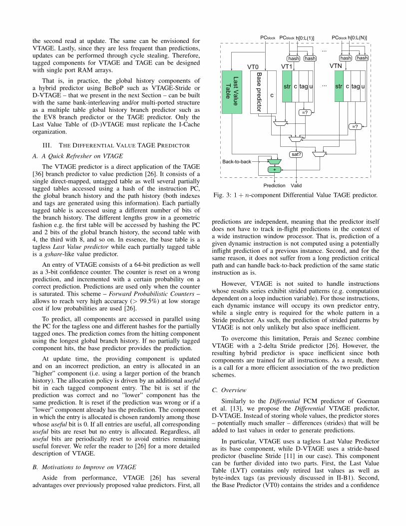
Fig. 3: 1 + n-component Differential Value TAGE predictor.

predictions are independent, meaning that the predictor itselfdoes not have to track in-flight predictions in the context ofa wide instruction window processor. That is, prediction of agiven dynamic instruction is not computed using a potentiallyinflight prediction of a previous instance. Second, and for thesame reason, it does not suffer from a long prediction criticalpath and can handle back-to-back prediction of the same staticinstruction as is.

However, VTAGE is not suited to handle instructionswhose results series exhibit strided patterns (e.g. computationdependent on a loop induction variable). For those instructions,each dynamic instance will occupy its own predictor entry,while a single entry is required for the whole pattern in aStride predictor. As such, the prediction of strided patterns byVTAGE is not only unlikely but also space inefficient.

To overcome this limitation, Perais and Seznec combineVTAGE with a 2-delta Stride predictor [26]. However, theresulting hybrid predictor is space inefficient since bothcomponents are trained for all instructions. As a result, thereis a call for a more efficient association of the two predictionschemes.

C. Overview

Similarly to the Differential FCM predictor of Goemanet al. [13], we propose the Differential VTAGE predictor,D-VTAGE. Instead of storing whole values, the predictor stores– potentially much smaller – differences (strides) that will beadded to last values in order to generate predictions.

In particular, VTAGE uses a tagless Last Value Predictoras its base component, while D-VTAGE uses a stride-basedpredictor (baseline Stride [11] in our case). This componentcan be further divided into two parts. First, the Last ValueTable (LVT) contains only retired last values as well asbyte-index tags (as previously discussed in II-B1). Second,the Base Predictor (VT0) contains the strides and a confidence

estimation mechanism. Both tables are direct-mapped but weuse small tags (e.g. 5 bits) on the LVT to maximize accuracy.

A 1 + n-component D-VTAGE is depicted in Fig. 3,assuming a single prediction per entry for clarity. Additionallogic with regard to VTAGE is shaded on the figure. Foreach fetch-block, the last values will be read from the LVT.Then, the strides will be selected depending on whether apartially tagged component hits, following the regular VTAGEoperation [26], [36]. If the same instruction block is fetchedtwice in two consecutive cycles, the predictions for the firstblock are bypassed to the input of the adders to be used as thelast values for the second block.

If the same instruction block is fetched twice in a singlecycle, both instances can be predicted by using 3-input adders(not shown in Fig. 3).

The advantages of D-VTAGE are twofold. First, it is ableto predict control-flow dependent patterns, strided patterns andcontrol-flow dependent strided patterns. Second, it has beenshown that short strides could capture most of the coverageof full strides in a stride-based value predictor [13]. As suchusing D-VTAGE instead of VTAGE, for instance, would allowto greatly reduce storage requirements.

D. Implementation Issues

a) Speculative History: Because of its stride-basednature, D-VTAGE relies on the value produced by the mostrecent instance of an instruction to compute the prediction forthe newly fetched instance. As many instances of the sameinstruction can coexist in the instruction window at the sametime, the hardware should provide some support to grab thepredicted value for the most recent speculative instance. Sucha hardware structure could be envisioned as a chronologicallyordered associative buffer whose size is roughly that of theROB. For instruction-based VP, such a design should proveslow and power hungry, e.g. more than ROB-size entries atworst and 8 parallel associative searches each cycle for thesimulation framework we are considering (8-wide, 6-issuesuperscalar).

Fortunately, BeBoP allows to greatly reduce the number ofrequired entries as well as the number of parallel accesses eachcycle since we group predictions per fetch block. We developsuch a design of the speculative window in Section IV.

b) Impact of Block-Based Prediction: As for VTAGEand TAGE, the allocation policy in the tagged componentsof D-VTAGE is driven by the usefulness of a prediction[36]. The allocation of a new entry also depends on whetherthe prediction was correct or not. However, we consider ablock-based predictor. Therefore, the allocation policy needs tobe modified since there can be correct and incorrect predictionsin a single entry, and some can be useful or not.

In our implementation, an entry is allocated if at least oneprediction in the block is wrong. However, the confidencecounter of predictions from the providing entry are propagatedto the newly allocated entry. This allows the predictor tobe efficiently trained (allocate on a wrong prediction) whilepreserving coverage since high confidence predictions areduplicated. The usefulness bit is kept per block and set if asingle prediction of the block is useful as defined in [26], that

is if it is correct and the prediction in the alternate componentis not.

c) Prediction Validation: The EOLE processor modelassumes that predictions are used only if they are very highconfidence. Therefore, unused predictions must be stored towait for validation in order to train the predictor. To thatextent, we assume a FIFO Update Queue where predictionblocks are pushed at prediction time and popped at validationtime. This structure can be read and written in the samecycle, but reads and writes are guaranteed not to conflict byconstruction. Specifically, this queue should be able to containall the predictions potentially in flight after the cycle in whichpredictions become available. It would also be responsible forpropagating any information visible at prediction time thatmight be needed at update time.

In essence, this structure is very similar to the speculativewindow that should be implemented for D-VTAGE. Indeed,it contains all the inflight predictions for each block, and itshould be able to rollback to a correct state on a pipeline flush(we describe recovery in the context of BeBoP in the nextSection). However, to maximize coverage, the FIFO updatequeue must be large enough so that prediction information isnever lost due to a shortage of free entries. On the contrary, wewill see that we can implement the speculative window withmuch less entries than the theoretical number of blocks thatcan be in flight at any given time. Moreover, the speculativewindow must be associatively searched every time a predictionblock is generated while the FIFO does not need associativelookup (except potentially for rollbacks). As a result, if bothstructures essentially store the same data, it is still interestingto implement them as two separate items.

IV. BLOCK-BASED SPECULATIVE WINDOW

In the context of superscalar processors where manyinstructions can be in flight, computational predictors such asD-VTAGE cannot only rely on their Last Value Table. Indeed,in the case where several instances of a loop body are live inthe pipeline, the last value required by the predictor may nothave been retired, or even computed. As a result, a speculativeLVT is required so that the predictor can keep up with theprocessor. Given the fact that an instruction is allowed to useits prediction only after several tens of previous instances havebeen correctly predicted (because of confidence estimation),keeping the predictor synchronized with the pipeline is evenmore critical. As a result, our third and last contribution dealswith the specific design of the Speculative Window.

An intuitive solution would consist in using an associativebuffer that can store all the in-flight predictions. On eachlookup, this buffer would be probed and provide the mostrecent prediction to be used as the last value, if any.Unfortunately, its size would be that of the ROB plus allinstructions potentially in flight between prediction availability(Rename) and Dispatch. Associative structures of this size –such as the Instruction Queue – are known to be slower thantheir RAM counterparts as well as power hungry [8], [16],[24].

Nonetheless, thanks to BeBoP, the number of requiredentries is actually much smaller than with instruction-basedVP, and the number of accesses is at most the number of

fetch blocks accessed in a given cycle. Furthermore, althoughthis buffer behaves as a fully associative structure for reads,it acts as a simple circular buffer for writes because it ischronologically ordered. That is, when the predictor provides anew prediction block, it simply adds it at the head of the buffer,without having to match any tag. If the head overlaps with thetail (e.g. if the buffer was dimensioned with too few entries),both head and tail are advanced. Lastly, partial tags (e.g. 15bits) can be used to match the blocks, as VP is speculative bynature (false positive is allowed).

To order the buffer and thus ensure that the most recententry is providing the last values if multiple entries hit, we cansimply use internal sequence numbers. In our experiments, weuse the sequence number of the first instruction of the block. Ablock-diagram of our speculative window is shown in Fig. 4.

A. Consistency of the Speculative History

Block-based VP entails intrinsic inconsistencies in thespeculative window. For instance, if a branch is predicted astaken, some predictions are computed while the instructionscorresponding to them have been discarded (the ones in thesame block as the branch but located after the branch).Therefore the speculative history becomes inconsistent evenif the branch is correctly predicted.

Moreover, pipeline squashing events may increase theimpact of such inconsistencies in the speculative window andthe FIFO update queue4. To illustrate why, let us denote thefirst instruction to be fetched after the pipeline flush as Inewand the instruction that triggered the flush as Iflush. Let usalso denote the fetch block address of Inew as Bnew and thatof Iflush as Bflush.

On a pipeline flush, all the entries whose associatedsequence number is strictly greater than that of Iflush arediscarded in both the speculative window and the FIFO updatequeue. The block at the head of both structures thereforecorresponds to Bflush. We must then consider if whether Inewbelongs to the same fetch block as Iflush or not. If not, thepredictor should operate as usual and provide a predictionblock for the new block, Bnew. If it does belong to the sameblock (i.e. Bflush equals Bnew), several policies are availableto us.

a) Do not Repredict and Reuse (DnRR): This policyassumes that all the predictions referring to Bflush/Bnew

are still valid after the pipeline flush. That is, Inew and allsubsequent instructions belonging to Bflush will be attributedpredictions from the prediction block that was generated whenBflush/Bnew was first fetched. Those predictions are availableat the head of the FIFO update queue. With this policy, theheads of the speculative history and FIFO update queue arenot discarded.

b) Do not Repredict and do not Reuse (DnRDnR):This policy is similar to DnRR except that all newly fetchedinstruction belonging to Bflush/Bnew will be forbidden to usetheir respective predictions. The reasoning behind this policyis that the case where Bnew equals Bflush typically happens

4In our implementation, each entry of the FIFO update queue is also taggedwith the internal sequence number of the first instruction in the fetch-blockto enable rollback.

Fig. 4: N-way speculative window. The priority encodercontrols the multiplexer by prioritizing the matching entrycorresponding to the most recent sequence number.

on a value misprediction, and if a prediction was wrong in theblock, chances are that the subsequent ones will too.

c) Repredict (Repred): This policy squashes the headsof the speculative history and FIFO update queue (theblocks containing Iflush). Then, once Inew is fetched, a newprediction block for Bflush/Bnew is generated. The idea isthat some prediction blocks might have retired since Iflushwas predicted, therefore, this new prediction block may notsuffer from an inconsistency due to the block-based speculativehistory.

d) Keep Older, Predict Newer (Ideal): This idealisticpolicy is able to keep the predictions pertaining to instructionsof block Bflush older than Iflush while generating newpredictions for Inew and subsequent instructions belonging toBnew. In essence, this policy assumes a speculative window(resp. FIFO update queue) that tracks predictions at theinstruction level, rather than the block level. As a result,the speculative window (resp. FIFO update queue) is alwaysconsistent.

V. EVALUATION METHODOLOGY

A. Simulator

We use the framework used by Perais and Seznec in [25] tovalidate the EOLE architecture. That is, a modified5 version ofthe gem5 cycle-level simulator [3] implementing the x86 64ISA. Note that contrarily to modern x86 implementations,gem5 does not support move elimination [9], [15], [28], µ-opfusion [12] and does not implement a stack-engine [12].

Table I describes our model: A relatively aggressive 4GHz,6-issue6 superscalar pipeline. The fetch-to-commit latency is20 cycles. The in-order front-end and in-order back-end areoverdimensioned to treat up to 8 µ-ops per cycle. We modela deep front-end (15 cycles) coupled to a shallow back-end (5cycles) to obtain a realistic branch/value misprediction penalty:

5Modifications mostly lie with the ISA implementation. In particular, weimplemented branches with a single µ-op instead of three and we removedsome false dependencies existing between instructions due to the way flagsare renamed/written.

6On our benchmark set and with our baseline simulator, an 8-issue machineachieves only marginal speedup over this baseline.

TABLE I: Simulator configuration overview. *not pipelined.

Front End

L1I 8-way 32KB, 1 cycle, Perfect TLB; 32B fetch buffer(two 16-byte blocks each cycle, potentially over one takenbranch) w/ 8-wide fetch, 8-wide decode, 8-wide rename; TAGE1+12 components 15K-entry total (' 32KB) [36], 20 cyclesmin. branch mis. penalty; 2-way 8K-entry BTB, 32-entry RAS.

Execution

192-entry ROB, 60-entry IQ unified, 72/48-entry LQ/SQ,256/256 INT/FP 4-bank register files; 1K-SSID/LFST StoreSets [6]; 6-issue, 4ALU(1c), 1MulDiv(3c/25c*), 2FP(3c),2FPMulDiv(5c/10c*), 2Ld/Str, 1Str; Full bypass; 8-wide WB,8-wide VP validation, 8-wide retire.

Caches

L1D 8-way 32KB, 4 cycles, 64 MSHRs, 2 reads and 2writes/cycle; Unified L2 16-way 1MB, 12 cycles, 64 MSHRs,no port constraints, Stride prefetcher, degree 8; All caches have64B lines and LRU replacement.

MemorySingle channel DDR3-1600 (11-11-11), 2 ranks, 8 banks/rank,8K row-buffer, tREFI 7.8us; Across a 64B bus; Min. Read Lat.:75 cycles, Max. 185 cycles.

20/21 cycles minimum. We allow two 16-byte blocks worthof instructions to be fetched each cycle, potentially over asingle taken branch. Table I describes the characteristics of thebaseline pipeline we use in more details. In particular, the OoOscheduler is dimensioned with a unified centralized 60-entryIQ and a 192-entry ROB on par with the latest commerciallyavailable Intel microarchitecture. We refer to this model as theBaseline 6 60 configuration (6-issue, 60-entry IQ).

As µ-ops are known at Fetch in gem5, all the widths givenin Table I are in µ-ops. Independent memory instructions (aspredicted by the Store Sets predictor [6]) are allowed to issueout-of-order. Entries in the IQ are released upon issue sinceselective replay is not needed on value mispredictions.

In the case where EOLE is used, we consider a1-deep, 8-wide Early Execution stage and an 8-wide LateExecution/Validation stage limited to 4 read ports per registerfile bank [25]. Lastly, if EOLE and VP are not used, theValidation and Late Execution stage is removed, yielding afetch-to-commit latency of 19 cycles. The minimum branchprediction penalty is kept at 20 cycles.

B. Value Predictor Operation

In its baseline version, the predictor makes a prediction atFetch for every eligible µ-op (i.e. producing a 64-bit or lessregister that can be read by a subsequent µ-op, as definedby the ISA implementation). To index the predictor, we XORthe PC of the x86 64 instruction with the µ-op index insidethat x86 64 instruction [25]. This avoids all µ-ops mapping tothe same entry, but may create aliasing. We assume that thepredictor can deliver fetch-width predictions each cycle. Thepredictor is updated in the cycle following retirement.

When using block-based prediction, the predictor is simplyaccessed with the PC of each fetch block and provides severalpredictions at once for those blocks. Similarly, update blocksare built after retirement and an entry is updated as soon as aninstruction belonging to a block different than the one beingbuilt is retired. Update can thus be delayed for several cycles.To maximize accuracy, we tag the LVT with 5 higher bits ofthe fetch block PC.

We transpose the configuration of VTAGE in [25] toD-VTAGE: 8K-entry base component with 6 1K-entry partiallytagged components. The partial tags are 13 bits for thefirst component, 14 for the second, and so on. Histories

TABLE II: Benchmarks used for evaluation. Top: CPU2000,Bottom: CPU2006. INT: 18, FP: 18, Total: 36.

Program Input IPC164.gzip (INT) input.source 60 0.845

168.wupwise (FP) wupwise.in 1.303171.swim (FP) swim.in 1.745172.mgrid (FP) mgrid.in 2.361173.applu (FP) applu.in 1.481

175.vpr (INT)net.in arch.in place.out dum.out -nodisp-place only -init t 5 -exit t 0.005 -alpha t0.9412 -inner num 2

0.668

177.mesa (FP) -frames 1000 -meshfile mesa.in -ppmfilemesa.ppm 1.021

179.art (FP)-scanfile c756hel.in -trainfile1 a10.img-trainfile2 hc.img -stride 2 -startx 110 -starty200 -endx 160 -endy 240 -objects 10

0.441

183.equake (FP) inp.in 0.655186.crafty (INT) crafty.in 1.562188.ammp (FP) ammp.in 1.258197.parser (INT) ref.in 2.1.dict -batch 0.486255.vortex (INT) lendian1.raw 1.526300.twolf (INT) ref 0.282

400.perlbench (INT) -I./lib checkspam.pl 2500 5 25 11 150 1 1 11 1.400

401.bzip2 (INT) input.source 280 0.702403.gcc (INT) 166.i 1.002

416.gamess (FP) cytosine.2.config 1.694429.mcf (INT) inp.in 0.113433.milc (FP) su3imp.in 0.501

435.gromacs (FP) -silent -deffnm gromacs -nice 0 0.753437.leslie3d (FP) leslie3d.in 2.151444.namd (FP) namd.input 1.781

445.gobmk (INT) 13x13.tst 0.733450.soplex (FP) -s1 -e -m45000 pds-50.mps 0.271453.povray (FP) SPEC-benchmark-ref.ini 1.465

456.hmmer (INT) nph3.hmm 2.037458.sjeng (INT) ref.txt 1.182

459.GemsFDTD (FP) / 1.146462.libquantum (INT) 1397 8 0.459

464.h264ref (INT) foreman ref encoder baseline.cfg 1.008470.lbm (FP) reference.dat 0.380

471.omnetpp (INT) omnetpp.ini 0.304473.astar (INT) BigLakes2048.cfg 1.165

482.sphinx3 (FP) ctlfile . args.an4 0.803483.xalancbmk (INT) -v t5.xml xalanc.xsl 1.835

range from 2 to 64 bits in a geometric fashion. We alsouse 3-bit Forward Probabilistic Counters with probabilitiesv = {1, 1

16 ,116 ,

116 ,

116 ,

132 ,

132}. Unless specified otherwise, we

use 64-bit strides in all the predictors we consider.

C. Benchmarks

We use a subset of the the SPEC’00 [37] and SPEC’06[38] suites to evaluate our contributions as we focus onsingle-thread performance. Specifically, we use 18 integerbenchmarks and 18 floating-point programs7. Table IIsummarizes the benchmarks we use as well as their input,which are part of the reference inputs provided in the SPECsoftware packages. To get relevant numbers, we identify aregion of interest in the benchmark using Simpoint 3.2 [27].We simulate the resulting slice in two steps: First, warm upall structures (caches, branch predictor and value predictor) for50M instructions, then collect statistics for 100M instructions.

7We do not use the whole suites due to some missing system calls/x87instructions in the gem5-x86 version we use in this study.

0.9

1

1.1

1.2

1.3

1.4

1.5

1.6

1.7

1.8

2d-Stride VTAGE VTAGE-2d-Stride D-VTAGE (Baseline_VP_6_60)

(a) Speedup obtained with different value predictors over Baseline 6 60.

0.95

1

1.05

1.1

1.15

1.2

1.25

EOLE_4_60 (w/ D-VTAGE)

(b) Speedup of bank/port constrained EOLE 4 60 [25] w/ D-VTAGE over Baseline VP 6 60.

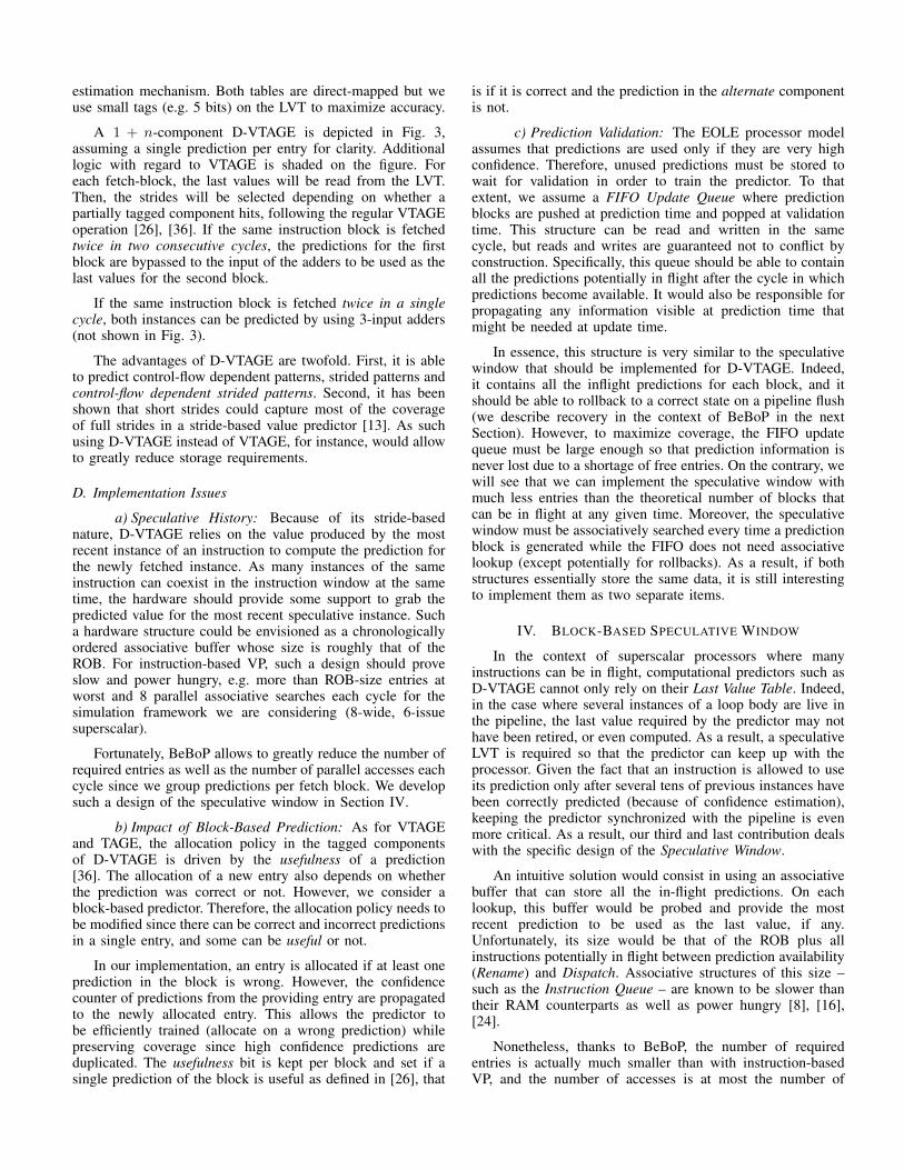
Fig. 5: Performance of D-VTAGE on a baseline 6-issue model and on a 4-issue EOLE pipeline.

D. A Remark on Power and Energy

In this work, we do not provide quantitative insights onpower and energy. However, we would like to stress thefollowing points.

Value Prediction as implemented in this paper decreasesenergy consumption because 1) Performance increases 2)The issue-width is reduced (thanks to EOLE). Moreover, thereduction in issue-width reduces power in the scheduler, whichis a well-known hotspot [8]. Conversely, it increases energyconsumption because of 1) The - simple - additional ALUsrequired by EOLE 2) The value predictor 3) The speculativevalue prediction window.

The value predictor itself is comparable in design (numberof tables, ports, storage volume, pressure) - and therefore inpower/energy consumption - to an aggressive branch predictor.An example of such an aggressive branch predictor – the2bc-gskew of the EV8 – required 44KB of storage [35]. InSection VI-C, we show that good performance is obtained with16 to 32KB of storage only.

Regarding the associative speculative window, we argue inSection VI-B that 32 entries is a good tradeoff. This is roughlytwo times fewer entries than Haswell’s scheduler. Assuming abaseline CAM-like scheduler and 6/8 results per cycle, theneach entry of the scheduler must provision 12/16 comparatorsfor wakeup, assuming 2 operands per entry (consider thatAMD Bulldozer’s actually has up to 4 per entry [14]). Thespeculative window only requires as many comparators perentry as there are blocks fetched per cycle (granted that thecomparators are bigger since we match 15 bits instead of 6-8).

That is, 64 15-bit comparators are needed as opposed to 7208-bit comparators for a 60-entry, 2 operands per entry, 6 resultsper cycle, 8-bit identifier scheduler. As a result, the complexityand power consumption of the speculative window should bemuch lower than those of the scheduler. Moreover, it wouldalways be possible to turn it off should the value predictorrarely hit in the speculative window (e.g. for a program withlarge loop bodies).

VI. EXPERIMENTAL RESULTS

In further experiments, when we do not give speedup foreach individual benchmark, we represent results using thegeometric mean of the speedups on top of the [Min,Max]box plot of the speedups.

A. Baseline Value Prediction

In this first set of experiments, we study the potential ofD-VTAGE without using BeBoP or EOLE in order to confirmthat it is a good candidate for a hybrid between VTAGEand Stride. We compare it to other similarly sized predictors(e.g. 8K-entry 2-delta Stride predictor and similarly laid outVTAGE).

Fig. 5 (a) demonstrates the potential of D-VTAGE onthe baseline model. First, no slowdown is observed withD-VTAGE. Second, D-VTAGE often performs better than anaive VTAGE-Stride hybrid [26] e.g. wupwise, swim, mgrid,applu, bzip, gamess, leslie and GemsFDTD. It is generallyon-par with said hybrid except in parser, gcc, astar andxalancbmk, although the difference in speedup remains limited

0.8

0.85

0.9

0.95

1

1.05

4p 1K +

6x128

6p 1K +

6x128

8p 1K +

6x128

4p 2K +

6x256

6p 2K +

6x256

8p 2K +

6x256

[Q1,Med] [Med,Q3] gmean

(a) Impact of the number of predictions per entry in D-VTAGE.

0.8

0.85

0.9

0.95

1

1.05

512 +

6x128

1K +

6x128

2K +

6x128

512 +

6x256

1K +

6x256

2K +

6x256

(b) Impact of the key structures sizes for a 6 predictions per entryD-VTAGE.

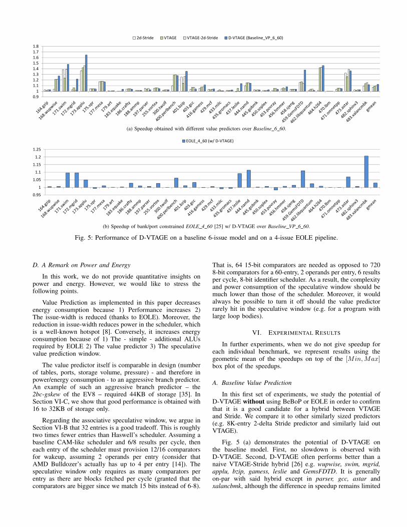
Fig. 6: Performance of D-VTAGE with BeBoP. Speedup overEOLE 4 60.

(4% at most in xalancbmk). As a result, we consider D-VTAGEto be a serious candidate for implementation, and in furtherexperiments, we focus on D-VTAGE only. In particular, werefer to the Baseline 6 60 configuration to which D-VTAGEis added as the Baseline VP 6 60 (6-issue, 60-entry IQ)configuration.

Fig. 5 (b) depicts the speedup of a 4-issue, 60-entry IQ,4-bank PRF, 12-read ports per bank EOLE architecture [25]featuring D-VTAGE over Baseline VP 6 60. We reproducethe results of Perais and Seznec in the sense that very littleslowdown is observed by scaling down the issue width from 6to 4 (at worst 0.982 in povray). We refer to this configuration asEOLE 4 60 and use it as our baseline in further experiments.

B. Block-Based Value Prediction

Fig. 6 (a) shows the impact of using BeBoP with D-VTAGEon top of EOLE 4 60. We respectively use 4, 6 and 8predictions per entry in the predictor, while keeping the sizeof the predictor roughly constant. For each configuration, westudy a predictor with either a 2K-entry base predictor and six256-entry tagged components or a 1K-entry base predictor andsix 128-entry tagged components. The Ideal policy is used tomanage the infinite speculative window.

We first make the observation that 6 predictions per 16-bytefetch block appear sufficient. Second, we note that reducingthe size of the structures plays a key role in performance. Forinstance, maximum slowdown is 0.876 for {6p 1K + 6x128},but only 0.957 for {6p 2K + 2x256}.

To gain further insight, in Fig. 6 (b), we focus on aD-VTAGE predictor with 6 predictions per entry and we varythe number of entries in the base component while keeping

0.9

0.95

1

1.05

Ideal Repred DnRDnR DnRR

[Q1,Med] [Med,Q3] gmean

(a) Impact of the recovery policy of the speculative window and FIFOupdate queue on speedup over EOLE 4 60.

0.8

0.85

0.9

0.95

1

1.05

∞ 64 56 48 32 16 None

(b) Impact of the size of the speculative window on speedup overEOLE 4 60. The recovery policy is DnRDnR.

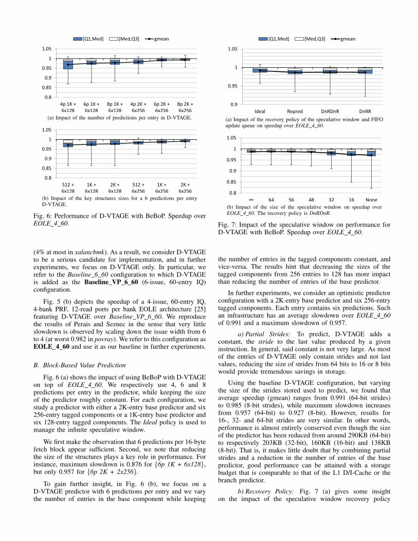
Fig. 7: Impact of the speculative window on performance forD-VTAGE with BeBoP. Speedup over EOLE 4 60.

the number of entries in the tagged components constant, andvice-versa. The results hint that decreasing the sizes of thetagged components from 256 entries to 128 has more impactthan reducing the number of entries of the base predictor.

In further experiments, we consider an optimistic predictorconfiguration with a 2K-entry base predictor and six 256-entrytagged components. Each entry contains six predictions. Suchan infrastructure has an average slowdown over EOLE 4 60of 0.991 and a maximum slowdown of 0.957.

a) Partial Strides: To predict, D-VTAGE adds aconstant, the stride to the last value produced by a giveninstruction. In general, said constant is not very large. As mostof the entries of D-VTAGE only contain strides and not lastvalues, reducing the size of strides from 64 bits to 16 or 8 bitswould provide tremendous savings in storage.

Using the baseline D-VTAGE configuration, but varyingthe size of the strides stored used to predict, we found thataverage speedup (gmean) ranges from 0.991 (64-bit strides)to 0.985 (8-bit strides), while maximum slowdown increasesfrom 0.957 (64-bit) to 0.927 (8-bit). However, results for16-, 32- and 64-bit strides are very similar. In other words,performance is almost entirely conserved even though the sizeof the predictor has been reduced from around 290KB (64-bit)to respectively 203KB (32-bit), 160KB (16-bit) and 138KB(8-bit). That is, it makes little doubt that by combining partialstrides and a reduction in the number of entries of the basepredictor, good performance can be attained with a storagebudget that is comparable to that of the L1 D/I-Cache or thebranch predictor.

b) Recovery Policy: Fig. 7 (a) gives some insighton the impact of the speculative window recovery policy

used for D-VTAGE with BeBoP. We assume an infinitespeculative window. In general the differences between therealistic policies are marginal, and on average, they behaveequivalently. As a result, we only consider DnRDnR as itreduces the number of predictor accesses versus Repred and itmarginally outperforms DnRR.

c) Speculative Window Size: Fig. 7 (b) illustratesthe impact of the speculative window size on D-VTAGE.When last values are not speculatively made available, somebenchmarks are not accelerated as much as in the infinitewindow case e.g. wupwise (0.914 vs. 0.984), applu (0.866vs. 0.996), bzip (0.820 vs. 0.998) and xalancbmk (0.923vs. 0.973). Having 56 entries in the window, however, providesroughly the same level of performance as an infinite number ofentries, while using only 32 entries appears as a good tradeoff(average performance is a slowdown of 0.980 for 32-entry and0.988 for ∞).

C. Putting it All Together

In previous experiments, we used a baseline EOLE 4 60model having a D-VTAGE predictor with 6 predictions perentry, a 2K-entry base component and six 256-entry taggedcomponents. Because it also uses 64-bit strides, it requiresroughly 290KB, not even counting the speculative window.Fortunately, we saw that the size of the base predictor could bereduced without too much impact on performance. Moreover,a speculative window with only a small number of entriesperforms well enough. Therefore, in this Section, we devisethree predictor configurations based on the results of previousexperiments as well as the observation that partial strides canbe used in D-VTAGE [13]. To obtain a storage budget weconsider reasonable, we use 6 predictions per entry and six128/256-entry tagged components. We then vary the size of thebase predictor, the speculative window, and the stride length.Table III reports the resulting configurations.

In particular, for Small (' 16KB), we also consider aversion with 4 predictions per entry but a base predictor twiceas big (Small 4p). For Medium (' 32KB), we found that bothtradeoffs have similar performance on average; for Large ('64KB), 4 prediction per entry perform worse than 6 on average,even with a 1K-entry base predictor. Thus, we do not reportresults for the hypothetical Medium 4p and Large 4p for thesake of clarity.

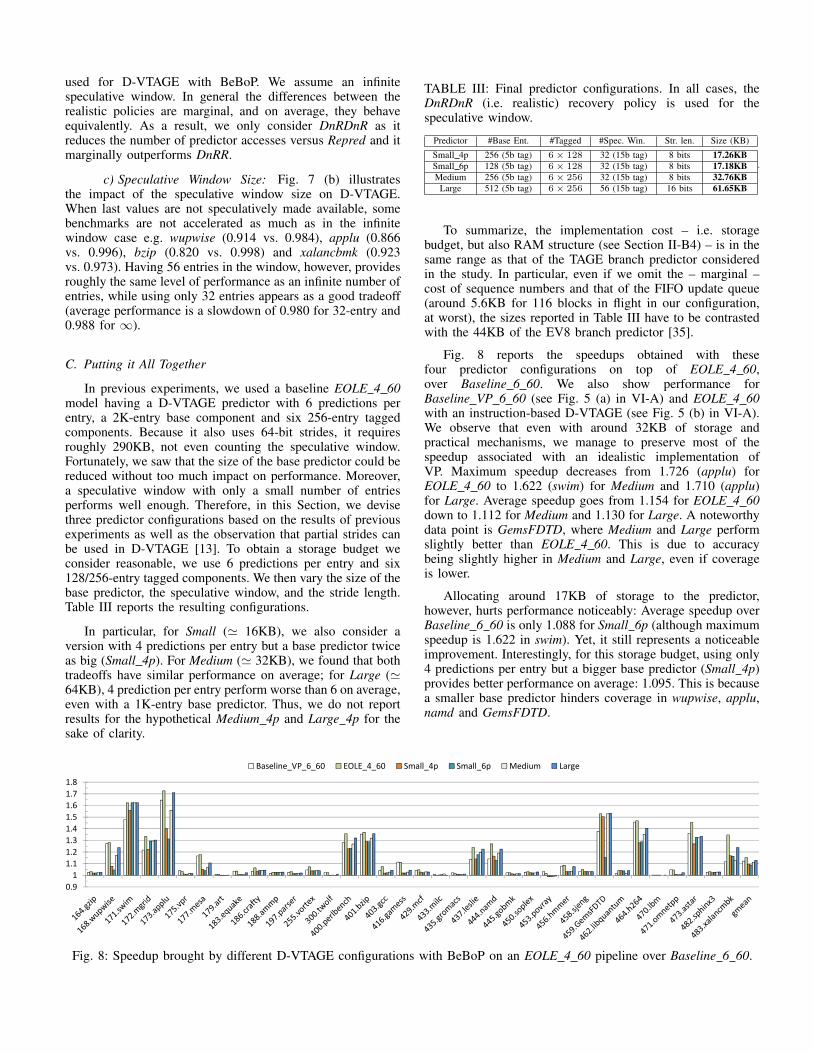
TABLE III: Final predictor configurations. In all cases, theDnRDnR (i.e. realistic) recovery policy is used for thespeculative window.

Predictor #Base Ent. #Tagged #Spec. Win. Str. len. Size (KB)

Small 4p 256 (5b tag) 6× 128 32 (15b tag) 8 bits 17.26KBSmall 6p 128 (5b tag) 6× 128 32 (15b tag) 8 bits 17.18KBMedium 256 (5b tag) 6× 256 32 (15b tag) 8 bits 32.76KB

Large 512 (5b tag) 6× 256 56 (15b tag) 16 bits 61.65KB

.

To summarize, the implementation cost – i.e. storagebudget, but also RAM structure (see Section II-B4) – is in thesame range as that of the TAGE branch predictor consideredin the study. In particular, even if we omit the – marginal –cost of sequence numbers and that of the FIFO update queue(around 5.6KB for 116 blocks in flight in our configuration,at worst), the sizes reported in Table III have to be contrastedwith the 44KB of the EV8 branch predictor [35].

Fig. 8 reports the speedups obtained with thesefour predictor configurations on top of EOLE 4 60,over Baseline 6 60. We also show performance forBaseline VP 6 60 (see Fig. 5 (a) in VI-A) and EOLE 4 60with an instruction-based D-VTAGE (see Fig. 5 (b) in VI-A).We observe that even with around 32KB of storage andpractical mechanisms, we manage to preserve most of thespeedup associated with an idealistic implementation ofVP. Maximum speedup decreases from 1.726 (applu) forEOLE 4 60 to 1.622 (swim) for Medium and 1.710 (applu)for Large. Average speedup goes from 1.154 for EOLE 4 60down to 1.112 for Medium and 1.130 for Large. A noteworthydata point is GemsFDTD, where Medium and Large performslightly better than EOLE 4 60. This is due to accuracybeing slightly higher in Medium and Large, even if coverageis lower.

Allocating around 17KB of storage to the predictor,however, hurts performance noticeably: Average speedup overBaseline 6 60 is only 1.088 for Small 6p (although maximumspeedup is 1.622 in swim). Yet, it still represents a noticeableimprovement. Interestingly, for this storage budget, using only4 predictions per entry but a bigger base predictor (Small 4p)provides better performance on average: 1.095. This is becausea smaller base predictor hinders coverage in wupwise, applu,namd and GemsFDTD.

0.9

1

1.1

1.2

1.3

1.4

1.5

1.6

1.7

1.8

Baseline_VP_6_60 EOLE_4_60 Small_4p Small_6p Medium Large

Fig. 8: Speedup brought by different D-VTAGE configurations with BeBoP on an EOLE 4 60 pipeline over Baseline 6 60.

As a result, we claim that BeBoP combined to D-VTAGEis an appealing possibility for an actual implementation of VP,even at reasonable storage budget (e.g. 16/32KB).

VII. RELATED WORK

A. Value Prediction

Lipasti et al. [19], [20] and Gabbay et al. [10], [11],[22] independently identify Value Locality and introduce ValuePrediction. Sazeides et al. [32] define two complementaryclasses of value predictors: Computational and Context-based.

Computational predictors generate a prediction by applyinga function to the value(s) produced by the previous instance(s)of the instruction, such as the addition of a constant(Stride predictor). Context-based predictors rely on patternsin the value history of a given static instruction to generatepredictions. The main representatives of this category are nthorder Finite Context Method predictors (FCM) [32]. Suchpredictors are usually implemented as two-level structures. Thefirst level (Value History Table or VHT) records a n-long valuehistory – possibly compressed – and is accessed using theinstruction address. The history is then hashed to form theindex of the second level (Value Prediction Table or VPT),which contains the actual prediction [4], [33]. The major hurdleof those predictors is the two-steps lookup. The predictioncritical path is too long to predict several instances of a staticinstruction in a short amount of time (e.g. tight loops). This isbecause the index computation of the 2nd level for the secondinstance has to wait for the first prediction [26].

Another avatar of – global – context-based value predictoris the VTAGE predictor introduced by Perais and Seznec in[26]. Here, the context consists of the global branch history andthe path history rather than local values. As a result, VTAGEdoes not require a speculative window to provide coherentpredictions, contrarily to most existing predictors. VTAGE hasbeen shown to perform better than a similarly sized order 4FCM [33], assuming around 256KB of storage. It can alsobe combined to a Stride-based predictor in order to maximizecoverage. Finally, VTAGE avoids the major shortcoming ofFCM-like predictors: a long prediction critical path. Therefore,it is able to seamlessly provide predictions for instructionsinside tight loops.

B. Hybrid Value Predictor Design

As computational and context-based predictors arecomplementary, many hybrid predictors have been developed.The simplest way to design a hybrid is to put twoor more predictors alongside and add a metapredictor toarbitrate. Since value predictors use confidence estimation,the metapredictor can be very simple e.g. never predict ifboth predictors are confident but disagree, otherwise use theprediction from the confident predictor. Yet, if components arecomplementary, there often is overlap: storage is wasted if aninstruction predictable by all components has an entry in everycomponent. Similarly, if an instruction is not predictable byone component, it is not efficient to let it occupy an entry insaid component. Rychlik et al. propose to use a classifier toattribute an instruction to one component at most [29]. Thisaddresses space-efficiency, but not complexity.

Goeman et al. [13] propose the Differential FCM predictor(D-FCM). They argue that storing strides instead of values inthe VHT and the VPT of FCM predictors allows to increasethe coverage of the predictor while also improving table usageefficiency. Such a predictor is a hybrid between a Stridepredictor and a baseline FCM predictor in the regular sense,but it actually combines the two prediction functions, allowingit to capture strided patterns that depend on the value history ofinstructions. Unfortunately, D-FCM suffers from the same longprediction critical path as FCM due to the two-level lookup andmay not be fit for practical implementation [26].

Another hybrid is the Per-Path Stride predictor (PS) ofNakra et al. [23]. In PS, the instruction address is used toaccess the last value in the Value History Table (VHT), whilethe stride is selected in the Stride History Table (SHT) using ahash of the global branch history and the PC. Then, both valuesare summed to form the prediction. This legitimizes the useof the global branch history to predict instruction results.

C. Predictor Storage & Complexity Reduction

To further improve space-efficiency, Sato et al. propose touse two tables for the Last Value Predictor (2-mode scheme)[30]. One contains full-width values and the other 8- or 16-bitvalues. At prediction time, both tables are accessed and theone with a tag match provides the prediction. Using 0/1-bitvalues is also a very space-efficient alternative [31].

Loh extends the 2-mode scheme by implementing severaltables of differing width [21]. The width of the resultis predicted by a simple classifier at prediction time.By serializing width-prediction and table access, a singleprediction table has to be accessed in order to predict. In bothcases, executing load immediate instructions for free in thefront-end overlaps with these propositions.

Burtscher et al. reduce the size of a Last n value predictorby noting that most of the high-order bits are shared betweenrecent values [5]. Hence, they only keep one full-width valueand the low-order bits of the n− 1 previous ones. Moreover,they remark that if n > 1, then a stride can be computed onthe fly, meaning that stride prediction can be done withoutadditional storage.

Finally, Lee et al. leverage trace processors to reducecomplexity [17]. They decouple the predictor from the Fetchstage: Predictions are attributed to traces by the fill unit.Thus, they solve the access latency and port arbitrationproblems on the predictor. They also propose some form ofblock-based prediction by storing predictions in the I-cache.[18]. However, a highly ported centralized structure is stillrequired to build predictions at retire-time. To address this,Bhargava et al. replace the value predictor by a PredictionTrace Queue that requires a single read port and a singlewrite port [2]. Lastly, Gabbay and Mendelson also devisea hardware structure to handle multiple prediction per cycleby using highly interleaved tables accessed with addresses ofinstructions in the trace cache [10]. Unfortunately, the scopeof all these studies except [18] is limited to trace processors.

VIII. CONCLUSION

Value Prediction is a very attractive technique to enhancesequential performance in a context where power efficiency

and cycle time entail that the instruction window cannotscale easily. However, many implementation details makeVP hard to imagine on real silicon. In recent work, Peraisand Seznec showed that a slow – but realistic – recoverymechanism can still yield speedup [26]. They also presenteda more practical predictor, VTAGE, that unfortunately cannotefficiently capture strided patterns. Then, by executing somesimple ready/predicted instructions early or late outside theOoO engine, they showed that issue width can be reduced,meaning that an implementation of VP with as many PRFports as a baseline superscalar can be envisioned. Saidimplementation would have a simpler Out-of-Order executionengine compared to a baseline superscalar processor [25].

In this work, we first described BeBoP, a block-basedprediction scheme adapted to complex variable-length ISAssuch as x86 as well as usually implemented fetch mechanism.BeBoP contributes to reducing the number of ports required onthe predictor by allowing several instructions to be predictedin a single access. Then, to reduce the footprint of thevalue predictor, we proposed a space-efficient hybrid ableto capture both strided patterns and control-flow dependentpatterns, D-VTAGE. We provided solutions for an actualimplementation of D-VTAGE. In particular, a small speculativewindow to handle in-flight instructions that only requires anassociative search on read operations, and a reduction in sizethanks to partial strides and smaller tables. In a nutshell, thehardware complexity of D-VTAGE is similar to that of anaggressive TAGE branch predictor.

As a result, this paper complements recent work andaddresses the remaining complexity involved with ValuePrediction. That is, the body of work consisting of [25], [26]and this paper provides one possible implementation of VP thatrequires less than 64KB of additional storage. The issue widthis even reduced when compared to the baseline 6-issue model.Nonetheless, this implementation of VP is able to speed upexecution by up to 62.2% with an average speedup of 11.2%while requiring only around 32KB of storage.

ACKNOWLEDGMENTS

This work was partially supported by the EuropeanResearch Council Advanced Grant DAL No. 267175.

REFERENCES

[1] Advanced Micro Devices, “AMD K6-III Processor Data Sheet,” pp.11–12, 1998.

[2] R. Bhargava and L. K. John, “Latency and energy aware valueprediction for high-frequency processors,” in Proceedings of theInternational Conference on Supercomputing, 2002, pp. 45–56.

[3] N. Binkert, B. Beckmann, G. Black, S. K. Reinhardt, A. Saidi, A. Basu,J. Hestness, D. R. Hower, T. Krishna, S. Sardashti, R. Sen, K. Sewell,M. Shoaib, N. Vaish, M. D. Hill, and D. A. Wood, “The gem5simulator,” SIGARCH Comput. Archit. News, vol. 39, no. 2, pp. 1–7,Aug. 2011.

[4] M. Burtscher, “Improving context-based load value prediction,” Ph.D.dissertation, University of Colorado, 2000.

[5] M. Burtscher and B. G. Zorn, “Hybridizing and coalescing loadvalue predictors,” in Proceedings of the International Conference onComputer Design, 2000, pp. 81–92.

[6] G. Z. Chrysos and J. S. Emer, “Memory dependence prediction usingstore sets,” in Proceedings of the International Symposium on ComputerArchitecture, 1998, pp. 142–153.

[7] R. Eickemeyer and S. Vassiliadis, “A load-instruction unit for pipelinedprocessors,” IBM Journal of Research and Development, vol. 37, no. 4,pp. 547–564, 1993.

[8] D. Ernst and T. Austin, “Efficient dynamic scheduling through tagelimination,” in Proceedings of the International Symposium onComputer Architecture, 2002, pp. 37–46.

[9] B. Fahs, T. Rafacz, S. J. Patel, and S. S. Lumetta, “Continuousoptimization,” in Proceedings of the International Symposium onComputer Architecture, 2005, pp. 86–97.

[10] F. Gabbay and A. Mendelson, “The effect of instruction fetch bandwidthon value prediction,” in Proceedings of The International Symposiumon Computer Architecture, 1998, pp. 272 –281.

[11] F. Gabbay and A. Mendelson, “Using value prediction to increase thepower of speculative execution hardware,” ACM Trans. Comput. Syst.,vol. 16, no. 3, pp. 234–270, Aug. 1998.

[12] S. Gochman, R. Ronen, I. Anati, A. Berkovits, T. Kurts, A. Naveh,A. Saeed, Z. Sperber, and R. C. Valentine, “The Intel PentiumM processor: Microarchitecture and performance,” Intel TechnologyJournal, vol. 7, May 2003.

[13] B. Goeman, H. Vandierendonck, and K. De Bosschere, “DifferentialFCM: Increasing value prediction accuracy by improving tableusage efficiency,” in Proceedings of the International Conference onHigh-Performance Computer Architecture, 2001, pp. 207–216.

[14] M. Golden, S. Arekapudi, and J. Vinh, “40-entry unified out-of-orderscheduler and integer execution unit for the AMD Bulldozer x86 64core,” in Solid-State Circuits Conference Digest of Technical Papers(ISSCC), 2011, pp. 80–82.

[15] S. Jourdan, R. Ronen, M. Bekerman, B. Shomar, and A. Yoaz, “A novelrenaming scheme to exploit value temporal locality through physicalregister reuse and unification,” in Proceedings of the InternationalSymposium on Microarchitecture, 1998, pp. 216–225.

[16] I. Kim and M. H. Lipasti, “Half-price architecture,” in Proceedingsof the International Symposium on Computer Architecture, 2003, pp.28–38.

[17] S.-J. Lee, Y. Wang, and P.-C. Yew, “Decoupled value prediction ontrace processors,” in Proceedings of the International Symposium onHigh-Performance Computer Architecture, 2000, pp. 231–240.

[18] S.-J. Lee and P.-C. Yew, “On table bandwidth and its update delayfor value prediction on wide-issue ilp processors,” Computers, IEEETransactions on, vol. 50, no. 8, pp. 847–852, 2001.

[19] M. H. Lipasti and J. P. Shen, “Exceeding the dataflow limit viavalue prediction,” in Proceedings of the International Symposium onMicroarchitecture, 1996, pp. 226–237.

[20] M. Lipasti, C. Wilkerson, and J. Shen, “Value locality and load valueprediction,” ASPLOS-VII, 1996.

[21] G. H. Loh, “Width prediction for reducing value predictor size andpower,” First Value Prediction Workshop, ISCA, 2003.

[22] A. Mendelson and F. Gabbay, “Speculative execution based onvalue prediction,” Technion-Israel Institute of Technology, Tech. Rep.TR1080, 1997.

[23] T. Nakra, R. Gupta, and M. Soffa, “Global context-based valueprediction,” in Proceedings of the International Symposium OnHigh-Performance Computer Architecture, 1999, pp. 4–12.

[24] S. Palacharla, N. Jouppi, and J. Smith, “Complexity-effectivesuperscalar processors,” in Proceedings of the International Symposiumon Computer Architecture, 1997, pp. 206–218.

[25] A. Perais and A. Seznec, “EOLE: Paving the way for an effectiveimplementation of value prediction,” in Proceedings of the InternationalSymposium on Computer Architecture, 2014.

[26] A. Perais and A. Seznec, “Practical data value speculation for futurehigh-end processors,” in Proceedings of the International Symposiumon High-Performance Computer Architecture, 2014.

[27] E. Perelman, G. Hamerly, and B. Calder, “Picking statistically valid andearly simulation points,” in Proceedings of the International Conferenceon Parallel Architectures and Compilation Techniques, 2003, pp. 244–.

[28] V. Petric, T. Sha, and A. Roth, “Reno: a rename-based instructionoptimizer,” in Proceedings of the International Symposium on ComputerArchitecture, 2005, pp. 98–109.

[29] B. Rychlik, J. Faistl, B. Krug, A. Kurland, J. Sung, M. Velev,and J. Shen, “Efficient and accurate value prediction using dynamicclassification,” Carnegie Mellon University, CMµART-1998-01, 1998.

[30] T. Sato and I. Arita, “Table size reduction for data value predictors byexploiting narrow width values,” in Proceedings of the InternationalConference on Supercomputing, 2000, pp. 196–205.

[31] T. Sato and I. Arita, “Low-cost value predictors using frequent valuelocality,” in High Performance Computing, 2002, pp. 106–119.

[32] Y. Sazeides and J. Smith, “The predictability of data values,” inProceedings of the International Symposium on Microarchitecture,1997, pp. 248–258.

[33] Y. Sazeides and J. Smith, “Implementations of context based valuepredictors,” Department of Electrical and Computer Engineering,University of Wisconsin-Madison, Tech. Rep. ECE97-8, 1998.

[34] A. Seznec, “A new case for the TAGE branch predictor,” in Proceedingsof the International Symposium on Microarchitecture, 2011, pp.117–127.

[35] A. Seznec, S. Felix, V. Krishnan, and Y. Sazeides, “Design tradeoffsfor the alpha EV8 conditional branch predictor,” in Proceedings ofthe Interational Symoposiumy on Computer Architecture, 2002, pp.295–306.

[36] A. Seznec and P. Michaud, “A case for (partially) TAgged GEometrichistory length branch prediction,” Journal of Instruction LevelParallelism, vol. 8, pp. 1–23, 2006.

[37] Standard Performance Evaluation Corporation. CPU2000. Available:http://www.spec.org/cpu2000/

[38] Standard Performance Evaluation Corporation. CPU2006. Available:http://www.spec.org/cpu2006/