UNIVERSIDADE FEDERAL DO RIO GRANDE DO SULINSTITUTO DE INFORMÁTICA

CURSO DE BACHARELADO EM CIÊNCIA DA COMPUTAÇÃO

VINICIUS MEDEIROS GRACIOLLI

Bedding Contact Detection: A movingmean-based approach

Work presented in partial fulfillmentof the requirements for the degree ofBachelor in Computer Science

Advisor: Prof. Dr. Mara AbelCoadvisor: Prof. Dr. Luis Fernando De Ros

Porto AlegreDecember 2014

UNIVERSIDADE FEDERAL DO RIO GRANDE DO SULReitor: Prof. Carlos Alexandre NettoVice-Reitor: Prof. Rui Vicente OppermannPró-Reitor de Graduação: Prof. Sérgio Roberto Kieling FrancoDiretor do Instituto de Informática: Prof. Luis da Cunha LambCoordenador do Curso de Ciência de Computação: Prof. Raul Fernando WeberBibliotecária-chefe do Instituto de Informática: Beatriz Regina Bastos Haro

“Eppur si muove.”— GALILEO GALILEI

THANKS

Joel CarboneraSandro Fiorini

Ana Julia Magnus de AssisLuan Garcia

Dean Pereira de MeloAndrius Jonuska

Nenad JaksicPetrobrás and ANP for providing testing data

CONTENTS

LIST OF ABBREVIATIONS AND ACRONYMS . . . . . . . . . . . . . . . . . . . 6

LIST OF SYMBOLS . . . . . . . . . . . . . . . . . . . . . . . . . . . . . . . . . . 7

ABSTRACT . . . . . . . . . . . . . . . . . . . . . . . . . . . . . . . . . . . . . . 8

RESUMO . . . . . . . . . . . . . . . . . . . . . . . . . . . . . . . . . . . . . . . . 9

LIST OF FIGURES . . . . . . . . . . . . . . . . . . . . . . . . . . . . . . . . . . . 10

LIST OF TABLES . . . . . . . . . . . . . . . . . . . . . . . . . . . . . . . . . . . 12

1 INTRODUCTION . . . . . . . . . . . . . . . . . . . . . . . . . . . . . . . . . 13

2 ROCK-LOG CORRELATION METHODS . . . . . . . . . . . . . . . . . . . . 182.1 Data Formats Used in This Work . . . . . . . . . . . . . . . . . . . . . . . . . 182.1.1 The LAS File . . . . . . . . . . . . . . . . . . . . . . . . . . . . . . . . . . . 182.1.2 The Strataledge Software . . . . . . . . . . . . . . . . . . . . . . . . . . . . . 182.2 Core Depth Adjustment . . . . . . . . . . . . . . . . . . . . . . . . . . . . . . 182.3 Deriving Rock Information From Wireline Logs . . . . . . . . . . . . . . . . 21

3 AUTOMATIC BEDDING DISCRIMINATOR . . . . . . . . . . . . . . . . . . . 243.1 Method . . . . . . . . . . . . . . . . . . . . . . . . . . . . . . . . . . . . . . . 243.2 Implementation . . . . . . . . . . . . . . . . . . . . . . . . . . . . . . . . . . . 273.2.1 Loading Data Structures . . . . . . . . . . . . . . . . . . . . . . . . . . . . . . 273.2.2 Cropping Logs . . . . . . . . . . . . . . . . . . . . . . . . . . . . . . . . . . . 273.2.3 Moving Means . . . . . . . . . . . . . . . . . . . . . . . . . . . . . . . . . . 283.2.4 Finding Break Points . . . . . . . . . . . . . . . . . . . . . . . . . . . . . . . 283.2.5 Comparing Break Points . . . . . . . . . . . . . . . . . . . . . . . . . . . . . 29

4 RESULTS . . . . . . . . . . . . . . . . . . . . . . . . . . . . . . . . . . . . . 324.1 Well ESS-0023 . . . . . . . . . . . . . . . . . . . . . . . . . . . . . . . . . . . 324.2 Well LPN-002 . . . . . . . . . . . . . . . . . . . . . . . . . . . . . . . . . . . . 334.3 Effects of Parameters in Contact Detection . . . . . . . . . . . . . . . . . . . 33

5 CONCLUSION . . . . . . . . . . . . . . . . . . . . . . . . . . . . . . . . . . . 45

REFERENCES . . . . . . . . . . . . . . . . . . . . . . . . . . . . . . . . . . . . . 46

LIST OF ABBREVIATIONS AND ACRONYMS

FMS Formation MicroScanner, a resistivity based image logging tool

UBI Ultrasonic Borehole Imager, a ultrasound based image logging tool

ANN Artificial Neural Network

BNN Bayesian Neural Network

LAS Log ASCII Standard

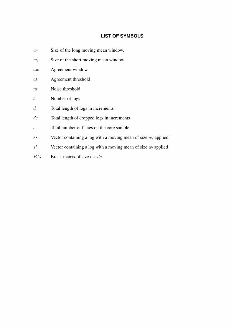
LIST OF SYMBOLS

wl Size of the long moving mean window.

ws Size of the short moving mean window.

aw Agreement window

at Agreement threshold

nt Noise threshold

l Number of logs

d Total length of logs in increments

dc Total length of cropped logs in increments

c Total number of facies on the core sample

ss Vector containing a log with a moving mean of size ws applied

sl Vector containing a log with a moving mean of size wl applied

BM Break matrix of size l × dc

ABSTRACT

This work discusses the importance of core-log integration and how the problem of coresample depth matching is such an integral part of this process. In order to align the depth ofcores and logs, it is required to identify some datum, or lithological contacts, that are stronglymarked both in cores and and geophysical logs. We revise here the current techniques used toperform depth matching and proposes a new method that can derive information about positionof contacts that can be used to perform core depth matching based on wireline log analysis.This method is based on moving means and works by detecting bedding planes across multiplelogs and by creating a unified assessment of lithology contacts, which can then be compared tocore sample descriptions. While the method shows some promise, the datasets used for testingwere were ill-suited for wireline log analysis and testing with data from logs with more welldefined and contrasting rocks is required for a more definitive proof of viability of this methodas a tool for core-log integration.

Keywords: Wireline log. core sample. depth matching. Strataledge. lithology prediction.

Detecção de planos de acabadamento: Uma abordagem com médias móveis

RESUMO

Este trabalho apresenta a importância da integração entre dados de perfil e de testemunho,e como o ajuste de profundidade do testemunho é uma parte integral deste processo. Paraalinhar a profundidade de perfis e testemunhos, é necessário identificar algum datum, ou contatolitológico, que é fortemente marcado em ambos os testemunhos e os perfis geofísicos. Sãodiscutidas as técnicas atuais utilizadas para ajuste de profundidade de testemunho e propostoum novo método que deriva informação sobre a posição de contatos de perfis geofísicos quepode ser utilizada para realizar o ajuste de profundidade de testemunho. Esse método é baseadoem médias móveis, e trabalha detectando limites entre camadas de rochas em múltiplos perfis;então unificando esta informação em uma avaliação total dos limites entre todos os perfis, quepode então ser comparada com as camadas de rocha descritas no testemunho. O método mostra-se promissor, porém, os dados disponíveis para teste são pouco adequados à análise de perfis,portanto, mais testes com dados mais adequados são necessários para se avaliar a viabilidadedo método e sua utilidade para a tarefa de ajuste de profundidade.

Palavras-chave: perfil geofísico. testemunho. ajuste de profundidade. Strataledge. prediçãolitológica.

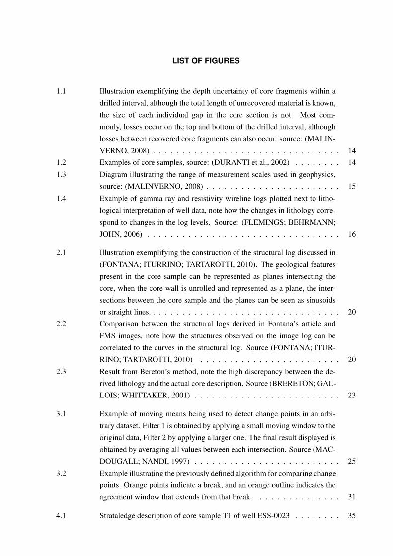
LIST OF FIGURES

1.1 Illustration exemplifying the depth uncertainty of core fragments within adrilled interval, although the total length of unrecovered material is known,the size of each individual gap in the core section is not. Most com-monly, losses occur on the top and bottom of the drilled interval, althoughlosses between recovered core fragments can also occur. source: (MALIN-VERNO, 2008) . . . . . . . . . . . . . . . . . . . . . . . . . . . . . . . . 14

1.2 Examples of core samples, source: (DURANTI et al., 2002) . . . . . . . . 14

1.3 Diagram illustrating the range of measurement scales used in geophysics,source: (MALINVERNO, 2008) . . . . . . . . . . . . . . . . . . . . . . . 15

1.4 Example of gamma ray and resistivity wireline logs plotted next to litho-logical interpretation of well data, note how the changes in lithology corre-spond to changes in the log levels. Source: (FLEMINGS; BEHRMANN;JOHN, 2006) . . . . . . . . . . . . . . . . . . . . . . . . . . . . . . . . . 16

2.1 Illustration exemplifying the construction of the structural log discussed in(FONTANA; ITURRINO; TARTAROTTI, 2010). The geological featurespresent in the core sample can be represented as planes intersecting thecore, when the core wall is unrolled and represented as a plane, the inter-sections between the core sample and the planes can be seen as sinusoidsor straight lines. . . . . . . . . . . . . . . . . . . . . . . . . . . . . . . . . 20

2.2 Comparison between the structural logs derived in Fontana’s article andFMS images, note how the structures observed on the image log can becorrelated to the curves in the structural log. Source (FONTANA; ITUR-RINO; TARTAROTTI, 2010) . . . . . . . . . . . . . . . . . . . . . . . . 20

2.3 Result from Bereton’s method, note the high discrepancy between the de-rived lithology and the actual core description. Source (BRERETON; GAL-LOIS; WHITTAKER, 2001) . . . . . . . . . . . . . . . . . . . . . . . . . 23

3.1 Example of moving means being used to detect change points in an arbi-trary dataset. Filter 1 is obtained by applying a small moving window to theoriginal data, Filter 2 by applying a larger one. The final result displayed isobtained by averaging all values between each intersection. Source (MAC-DOUGALL; NANDI, 1997) . . . . . . . . . . . . . . . . . . . . . . . . . 25

3.2 Example illustrating the previously defined algorithm for comparing changepoints. Orange points indicate a break, and an orange outline indicates theagreement window that extends from that break. . . . . . . . . . . . . . . 31

4.1 Strataledge description of core sample T1 of well ESS-0023 . . . . . . . . 35

4.2 Bedding planes inferred by analysis of wireline logs in well ESS-0023, coreT1 is displayed on the right. Note that only the bedding planes are shownon the core, the colors on the core are not representative of lithotype, theyonly show where the lithology changes. . . . . . . . . . . . . . . . . . . . 36

4.3 Parameter used in core T1, well ESS-0023 . . . . . . . . . . . . . . . . . 364.4 Strataledge description of core sample T1 of well ESS-0023 . . . . . . . . 374.5 Bedding planes inferred by analysis of wireline logs in well ESS-0023, core

T2 is displayed on the right. Note that only the bedding planes are shownon the core, the colors on the core are not representative of lithotype, theyonly show where the lithology changes. . . . . . . . . . . . . . . . . . . . 38

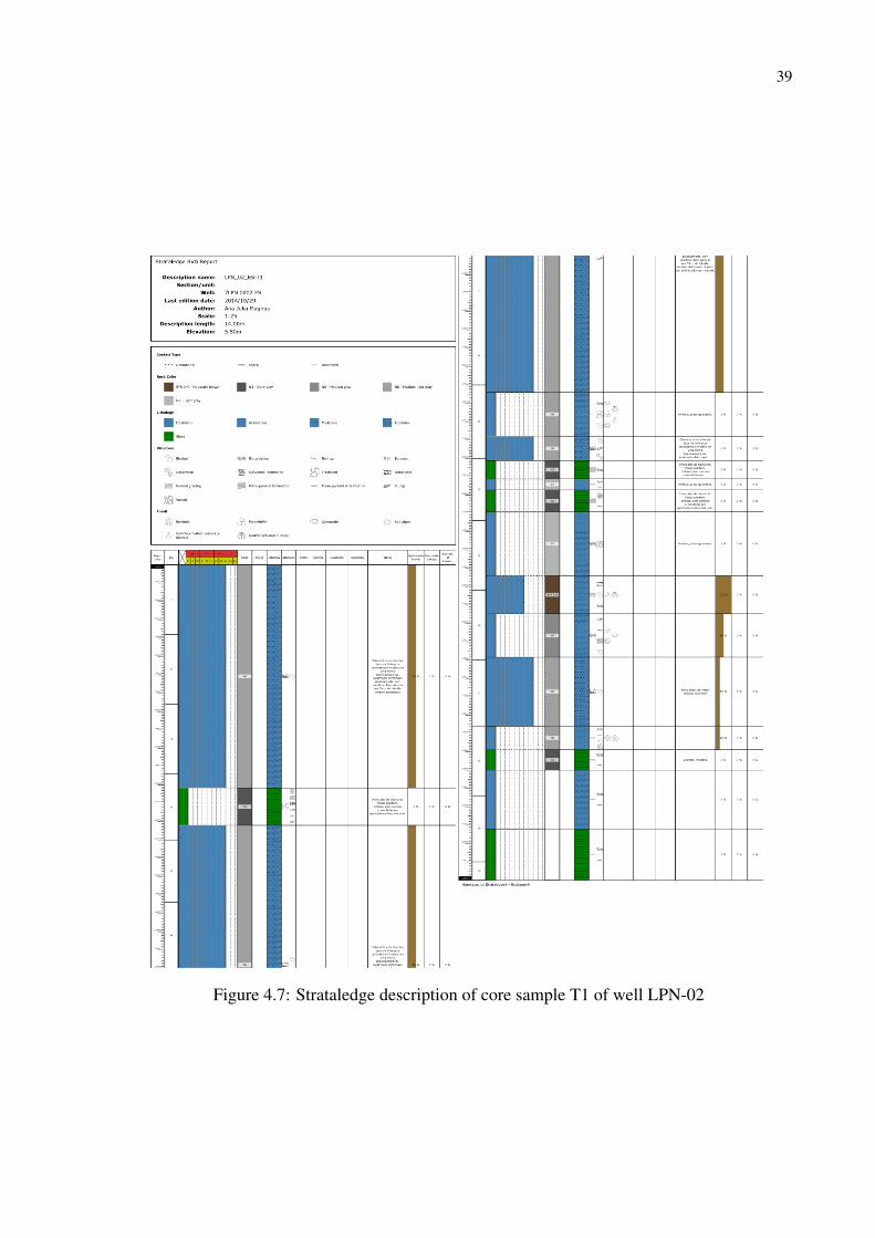
4.6 Parameter used in core T1, well ESS-0023 . . . . . . . . . . . . . . . . . 384.7 Strataledge description of core sample T1 of well LPN-02 . . . . . . . . . 394.8 Bedding planes inferred by analysis of wireline logs in well LPN-02, core

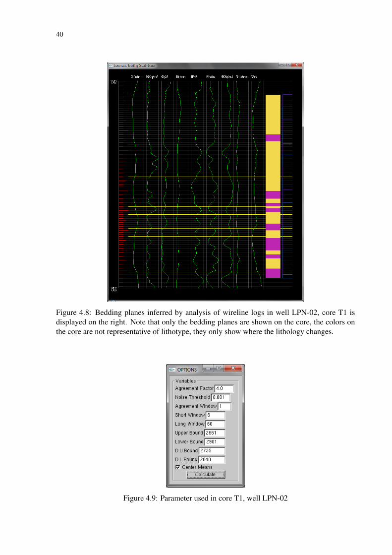
T1 is displayed on the right. Note that only the bedding planes are shownon the core, the colors on the core are not representative of lithotype, theyonly show where the lithology changes. . . . . . . . . . . . . . . . . . . . 40

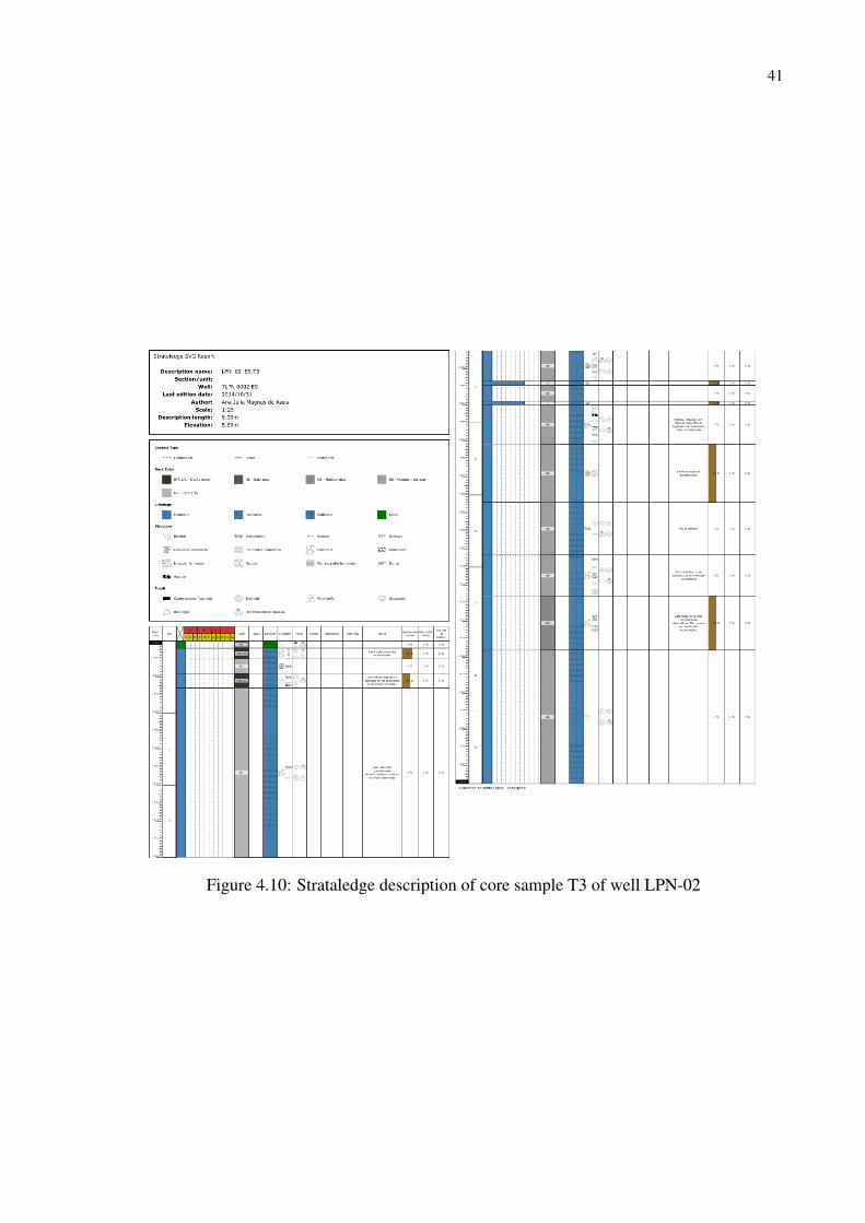
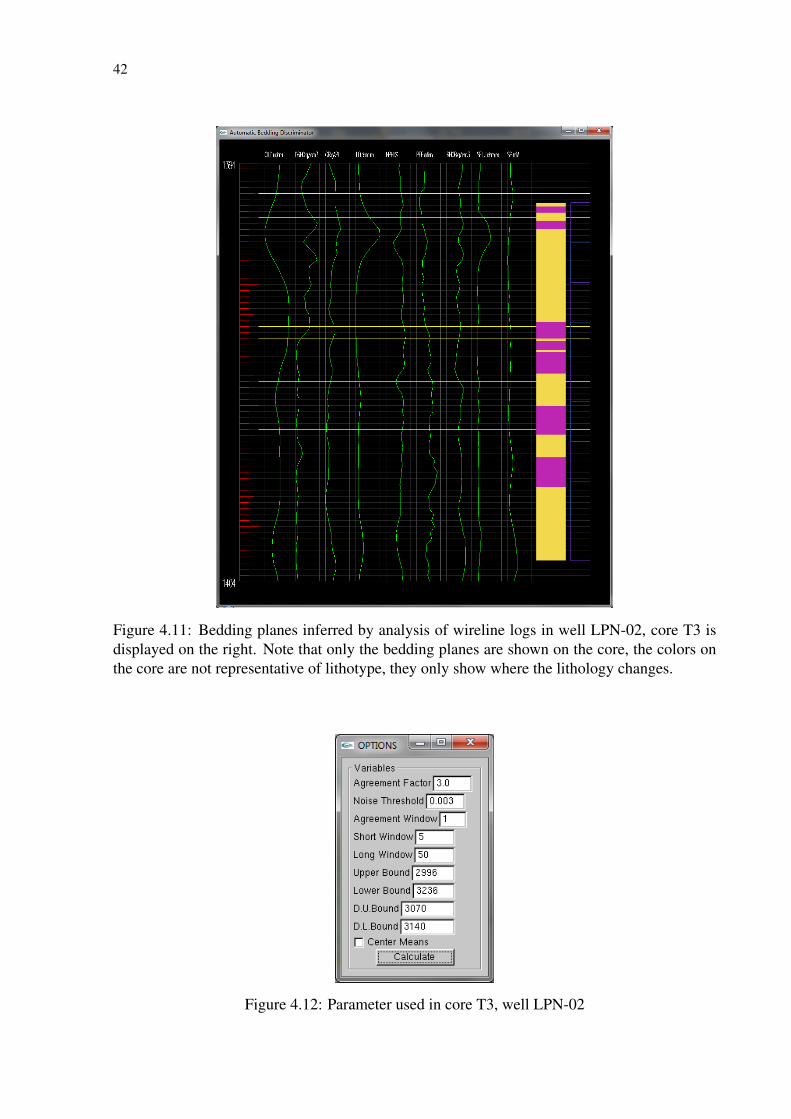
4.9 Parameter used in core T1, well LPN-02 . . . . . . . . . . . . . . . . . . . 404.10 Strataledge description of core sample T3 of well LPN-02 . . . . . . . . . 414.11 Bedding planes inferred by analysis of wireline logs in well LPN-02, core

T3 is displayed on the right. Note that only the bedding planes are shownon the core, the colors on the core are not representative of lithotype, theyonly show where the lithology changes. . . . . . . . . . . . . . . . . . . . 42

4.12 Parameter used in core T3, well LPN-02 . . . . . . . . . . . . . . . . . . . 42

LIST OF TABLES

4.1 Weights used for logs on well ESS-0023 . . . . . . . . . . . . . . . . . . . 434.2 Weights used for logs on well LPN-02 . . . . . . . . . . . . . . . . . . . . 434.3 Breakdown of the results shown in this chapter. . . . . . . . . . . . . . . . 44

13

1 INTRODUCTION

In the field of petroleum exploration and development, exploration wells provide importantinformation about the potential production of reservoirs, since they allow direct access to therock properties. These properties define the quality of a particular reservoir, as well as pro-vide us with geological information regarding the surrounding areas, which can be useful forgeological and stratigraphic interpretation of the surrounding region.

As a common process, exploration logs provide several objects of study. The first are thegeophysical logs, which are physical measures taken along of the whole deep of the well, suchas emission of gamma rays, variation of electrical resistivity of the rocks, acoustic transmissionand many others. The second is the drill cuttings that are taken out of the well along with theperforation water. The small cuts of rock provide a general view of the lithology that is beingcutting by the perforation. The third object of study are core samples, that due to the price ofrecovery, are taken only from intervals of interest along the well, usually the reservoir rock andthe rock seal that traps the oil in place (HYNE, 2012).

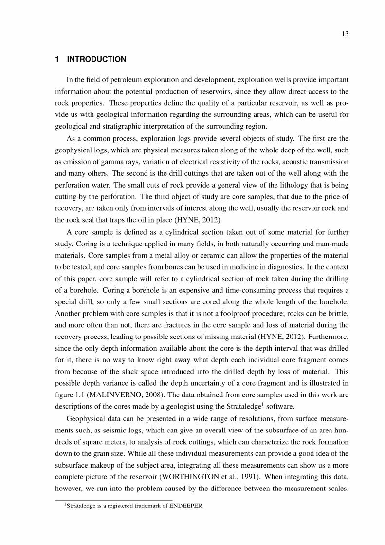
A core sample is defined as a cylindrical section taken out of some material for furtherstudy. Coring is a technique applied in many fields, in both naturally occurring and man-madematerials. Core samples from a metal alloy or ceramic can allow the properties of the materialto be tested, and core samples from bones can be used in medicine in diagnostics. In the contextof this paper, core sample will refer to a cylindrical section of rock taken during the drillingof a borehole. Coring a borehole is an expensive and time-consuming process that requires aspecial drill, so only a few small sections are cored along the whole length of the borehole.Another problem with core samples is that it is not a foolproof procedure; rocks can be brittle,and more often than not, there are fractures in the core sample and loss of material during therecovery process, leading to possible sections of missing material (HYNE, 2012). Furthermore,since the only depth information available about the core is the depth interval that was drilledfor it, there is no way to know right away what depth each individual core fragment comesfrom because of the slack space introduced into the drilled depth by loss of material. Thispossible depth variance is called the depth uncertainty of a core fragment and is illustrated infigure 1.1 (MALINVERNO, 2008). The data obtained from core samples used in this work aredescriptions of the cores made by a geologist using the Strataledge1 software.

Geophysical data can be presented in a wide range of resolutions, from surface measure-ments such, as seismic logs, which can give an overall view of the subsurface of an area hun-dreds of square meters, to analysis of rock cuttings, which can characterize the rock formationdown to the grain size. While all these individual measurements can provide a good idea of thesubsurface makeup of the subject area, integrating all these measurements can show us a morecomplete picture of the reservoir (WORTHINGTON et al., 1991). When integrating this data,however, we run into the problem caused by the difference between the measurement scales.

1Strataledge is a registered trademark of ENDEEPER.

14

Figure 1.1: Illustration exemplifying the depth uncertainty of core fragments within a drilledinterval, although the total length of unrecovered material is known, the size of each individualgap in the core section is not. Most commonly, losses occur on the top and bottom of the drilledinterval, although losses between recovered core fragments can also occur. source: (MALIN-VERNO, 2008)

Figure 1.2: Examples of core samples, source: (DURANTI et al., 2002)

15

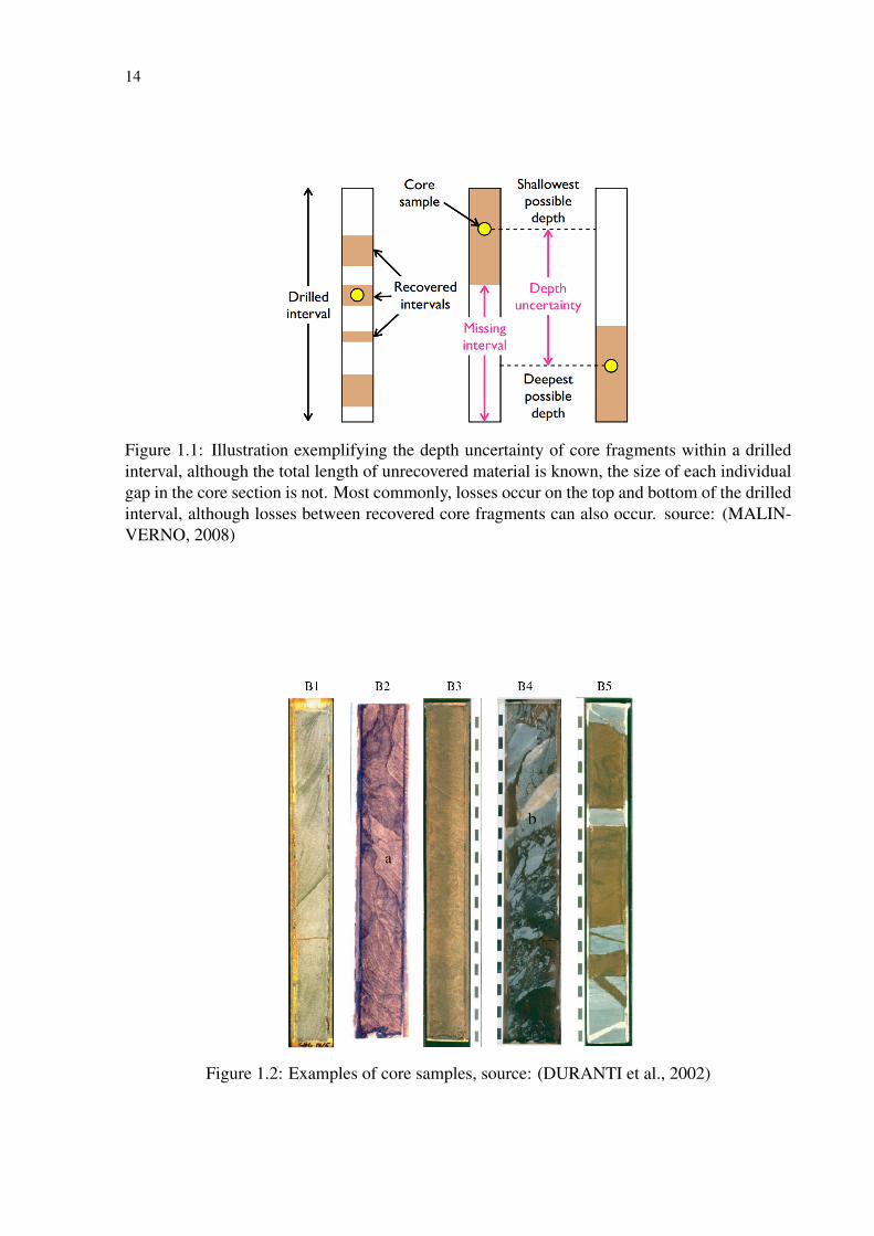
The information that may seem a small offset between two sets of data from the point of viewof the larger scale measurement may line up the smaller scale with a reading that makes nosense. These offsets are very common since measurements are taken at different times andusing different tools (LOFTS; BRISTOW, 1998).

Figure 1.3: Diagram illustrating the range of measurement scales used in geophysics, source:(MALINVERNO, 2008)

Wireline logs are measurements taken along the length of the borehole, either during drillingby tools that are attached to the drilling head (LWD) or after it is drilled by tools lowered intothe borehole (Wireline). For simplicity purposes, we will refer to measurements taken with anyof these tools as wireline logs. These tools can be classified as passive, where they just takemeasurements from the borehole such as natural gamma ray emissions, or active, where theyexcite the rock in some way and then measure a response, like the neutron porosity tool, whichemits neutrons and records the returning neutrons or gamma radiation. These log measurementsmay be further classified in uncased and cased measurements, with the former being taken froman open borehole, and the latter being taken after the borehole has been cased with piping.Wireline logs are presented as a table of depths and the values measured by each of the loggingtools used at each depth increment (KRYGOWSKI, 2003).

Depth data from logging runs is still prone to error, the tool may get stuck while it is be-ing pulled up from the well and record data from the same depth multiple times, after gettingunstuck it can also come up too fast due to cable tension and miss certain depths. Additionalproblems arise on underwater wells, where the waves can cause the logging ship to heave andalter the depth of the logging tool. Furthermore, if multiple logging runs are done on the samewell, some processing must be done in order to line up the depths recorded by the differentruns, usually one of the tools is used across all the runs and used as reference, most frequently,the gamma ray tool. These problems are best and usually handled by the logging companyitself during data acquisition, so, the data used in this work will be considered correct (LOFTS;BRISTOW, 1998).

16

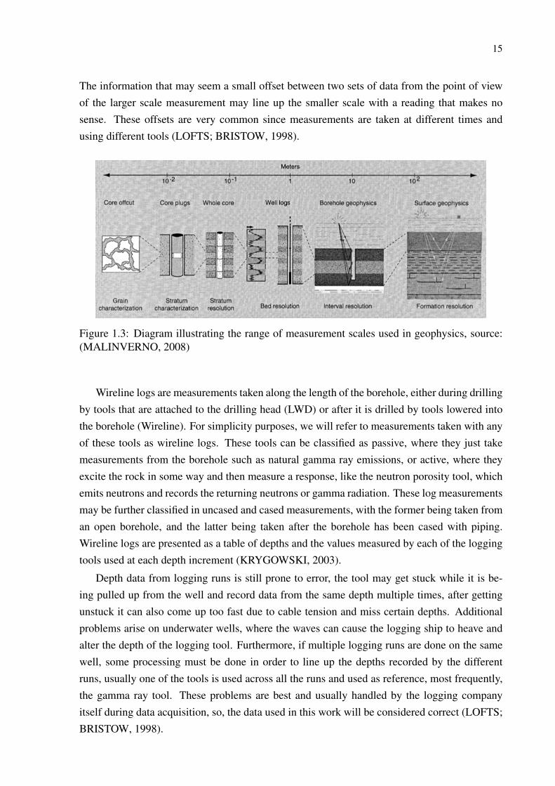
Figure 1.4: Example of gamma ray and resistivity wireline logs plotted next to lithologicalinterpretation of well data, note how the changes in lithology correspond to changes in the loglevels. Source: (FLEMINGS; BEHRMANN; JOHN, 2006)

17

In this work, I will focus on the depth matching step of integration of core sample descrip-tions and wireline-log data. We can define the problem of core depth-matching as assigningto each core sample fragment it’s real depth within the drilled depth, using the wireline logsas reference to make that assessment. Although there are plenty of efforts done by softwareprovider companies, to this day, this is still a task performed manually by a specialist, relyingon more information than what is being used in this work, such as geophysical measurementsof the core sample, or resistivity images from the borehole wall.

The aim of this work is not to replace the expert guided work, but to offer an alternativemethod of adjustment to support non-specialized geologists in adjusting the core depth andcorrelating wells by providing qualified rock data and semi-automatic methods of depth adjust-ment.

18

2 ROCK-LOG CORRELATION METHODS

This chapter revises the main methods described in literature for core depth adjustment androck-log correlation in exploration wells. The description of the approach used in each methodis followed by an evaluation of the effectiveness of the proposal.

2.1 Data Formats Used in This Work

This section describes the data formats used in this work to retrieve data regarding well logsand core sample descriptions. Their usage will be described in the next chapter.

2.1.1 The LAS File

The Log ASCII Standard (LAS) file is the current industry standard for storing and trans-mitting borehole log information. A LAS file usually consists of the following (CRANGLE,2007):

1. A header detailing the LAS version the file is formatted as.

2. The well information section, dealing in general well information such as geographicalcoordinates, depth drilled and companies responsible for drilling and logging.

3. The curve information section, which lists which measurements are logged in the file.

4. The ASCII log data section, which lists the values measured at each depth increment forevery curve in the log, in the same order as described in the curve information section.

2.1.2 The Strataledge Software

Core sample descriptions are the result of visual inspection by a geologist, who will drawand write down what attributes he sees on the sample. This can create a lot of ambiguity, sincedifferent geologists and companies can have their own way of drawing structures and a differentlexicon to describe them.

The Strataledge software (PERRIN et al., 2012) provides a standardized ontology basedenvironment where the geologist can describe the core sample using standardized names andrepresentations based on a well-founded ontology. This description can then be exported as anSVG file for human inspection, or as an XML file for processing.

2.2 Core Depth Adjustment

Since core depth matching is a problem under study for decades, many techniques havebeen proposed over the years to tackle this issue. Most of these methods disregard the coresample descriptions used in this work and instead opt to extract geophysical data from the core

19

samples using objective measurement tools. These kind of approaches give you the advantageof comparing two sets of numerical data, instead of one set of numerical data and a qualitativedescription that is open to interpretation.

The current standard procedure in the petroleum industry consists in taking the gammaray measurements from the core sample using a gamma ray logger and comparing it with thegamma ray measurements obtained from the wireline tools. It is up to the geologist to findthe depths where the two curves have the best match. (MORTON-THOMPSON; WOODS;GEOLOGISTS, 1993)

Another method, patented by Vinegar et al. (VINEGAR; WELLINGTON, 1985) revolvesaround the use of a computerized axial tomographic scanner (CAT) to determine the attenuationcoefficients at a plurality of cross sections along the core sample. Since the attenuation coef-ficients are directly proportional to the density values of the core, these values can be interpo-lated and convolved with the response function of a density logging tool to generate convolveddensity values that can be compared to bulk density data obtained from wireline tools. An-other embodiment of the same method involves convolving effective atomic numbers with theresponse function of the tool to obtain convolved effective atomic numbers that are cross corre-lated with the photoelectric log values. In either case, values on both sets of data are comparedby a specialist who determines the best depth shift on the core.

A patent made in 2005 by Siddiqui (SIDDIQUI, 2005) builds upon Vinegar’s work. Itaims to simplify the calculations involved by using standardized CT number data and statisticalanalysis to calculate the core’s bulk density, instead of using the tool response function.

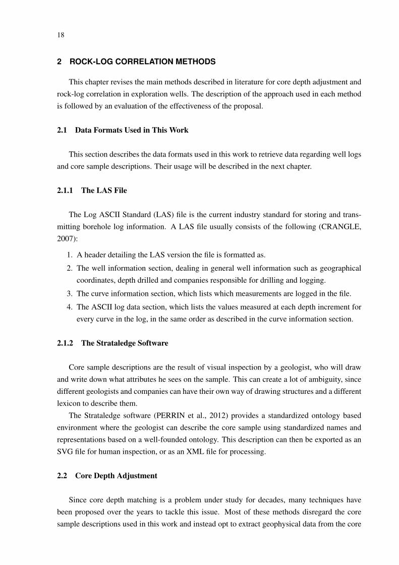
Techniques that do not rely on core geophysical data have also been developed over theyears, Fontana et al. (FONTANA; ITURRINO; TARTAROTTI, 2010) describes a way to derivea core image from a mathematical representation of the core sample:

We assume that the geological structures described in the structural logs are

planar features and the borehole wall is a cylinder. Considering the unrolled sur-

face of the borehole wall, any intersection of a structure and the borehole wall can

then be represented by:

1. a sinusoid (structure neither normal nor parallel to the borehole axis),

2. a horizontal straight line (horizontal structure, normal to the borehole axis),

3. or a vertical straight line (vertical structure, parallel to the borehole axis)

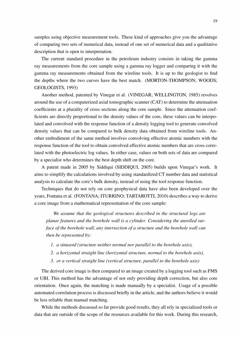
The derived core image is then compared to an image created by a logging tool such as FMSor UBI. This method has the advantage of not only providing depth correction, but also coreorientation. Once again, the matching is made manually by a specialist. Usage of a possibleautomated correlation process is discussed briefly in the article, and the authors believe it wouldbe less reliable than manual matching.

While the methods discussed so far provide good results, they all rely in specialized tools ordata that are outside of the scope of the resources available for this work. During this research,

20

Figure 2.1: Illustration exemplifying the construction of the structural log discussed in(FONTANA; ITURRINO; TARTAROTTI, 2010). The geological features present in the coresample can be represented as planes intersecting the core, when the core wall is unrolled andrepresented as a plane, the intersections between the core sample and the planes can be seen assinusoids or straight lines.

Figure 2.2: Comparison between the structural logs derived in Fontana’s article and FMS im-ages, note how the structures observed on the image log can be correlated to the curves in thestructural log. Source (FONTANA; ITURRINO; TARTAROTTI, 2010)

21

we found no literature on solving depth matching using only wireline logs and core descriptions,so a new method has to be proposed.

2.3 Deriving Rock Information From Wireline Logs

The main obstacle to overcome when integrating wireline data and core descriptions rests inbridging the gap between a numeric value and a qualitative description. To do that, we need toprocess one of the data sets and make it comparable to the other. Taking a qualitative descriptionand simulating a wireline log based on the description is not a reliable process, since not onlyreadings for the same type of rock can vary wildly between different wells, but also somereadings may have no direct correlation to the lithology observed (MANN; LEYTHAEUSER;MÜLLER, 1986). Therefore, it is a more interesting approach to process the wireline logs andlook for markers that can be correlated to the core description.

Neural networks have been used in this field to predict lithology with varying degrees ofsuccess. An artificial neural network (ANN) is a computational model inspired by an animal’snervous system. In its most basic form, an ANN is presented as a system of interconnectednodes (neurons). The connections between neurons have assigned weights that are tuned by alearning algorithm in such a way that the final output of the neural network matches the expectedresult. In the context of this work, an example would be a neural network whose input neuronsreceive the measured wireline log values at a certain depth, apply an evaluation function to thesevalues and propagate the results to the adjacent neurons. These neuron, in turn, do the sameprocess until an output neuron is activated, whose final value is the estimated lithology at thatdepth.

The learning algorithms used in neural networks can be supervised or unsupervised. On su-pervised learning, the algorithm is fed a set of sample pairs consisting of previously determinedinputs and their associated outputs. The aim of the learning algorithm is then to estimate whichfunction that correctly maps the input value to the output value. On unsupervised learning, thealgorithm receives input data and a cost function to minimize.

Ojha (OJHA; MAITI, 2013) shows an approach using a Bayesian Neural Network (BNN)that differs from a regular ANN by virtue of the heuristic used to choose the starting values forthe network weights. While an ANN picks a single set w0 of starting weighs randomly, a BNNconsiders the entire space w of possible weight assignments and performs a weighted averageacross the whole domain using supervised learning. The data sets used for supervised learningon Ojha’s work are derived from clustering and statistical analysis methods applied to wirelinelog data. The article claims an average accuracy of 67.38% in the presence of 10% red noise.The problem in using this approach as a way of comparing wireline and core data is that thetraining process must be redone for every individual well. Also, that training requires someprior knowledge about the well, such as how many different lithologies are represented on thelogs so that the clustering methods may be applied.

22

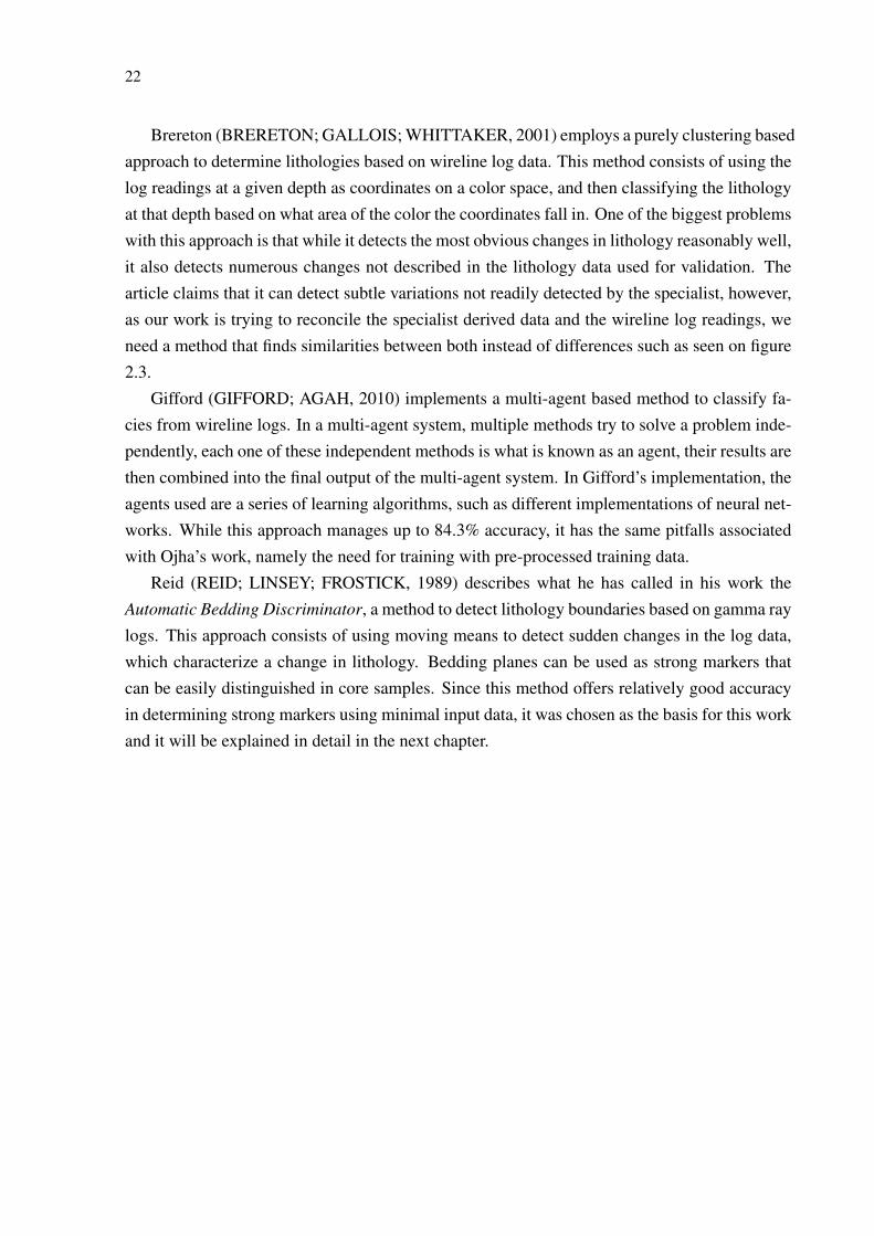
Brereton (BRERETON; GALLOIS; WHITTAKER, 2001) employs a purely clustering basedapproach to determine lithologies based on wireline log data. This method consists of using thelog readings at a given depth as coordinates on a color space, and then classifying the lithologyat that depth based on what area of the color the coordinates fall in. One of the biggest problemswith this approach is that while it detects the most obvious changes in lithology reasonably well,it also detects numerous changes not described in the lithology data used for validation. Thearticle claims that it can detect subtle variations not readily detected by the specialist, however,as our work is trying to reconcile the specialist derived data and the wireline log readings, weneed a method that finds similarities between both instead of differences such as seen on figure2.3.

Gifford (GIFFORD; AGAH, 2010) implements a multi-agent based method to classify fa-cies from wireline logs. In a multi-agent system, multiple methods try to solve a problem inde-pendently, each one of these independent methods is what is known as an agent, their results arethen combined into the final output of the multi-agent system. In Gifford’s implementation, theagents used are a series of learning algorithms, such as different implementations of neural net-works. While this approach manages up to 84.3% accuracy, it has the same pitfalls associatedwith Ojha’s work, namely the need for training with pre-processed training data.

Reid (REID; LINSEY; FROSTICK, 1989) describes what he has called in his work theAutomatic Bedding Discriminator, a method to detect lithology boundaries based on gamma raylogs. This approach consists of using moving means to detect sudden changes in the log data,which characterize a change in lithology. Bedding planes can be used as strong markers thatcan be easily distinguished in core samples. Since this method offers relatively good accuracyin determining strong markers using minimal input data, it was chosen as the basis for this workand it will be explained in detail in the next chapter.

23

Figure 2.3: Result from Bereton’s method, note the high discrepancy between the derived lithol-ogy and the actual core description. Source (BRERETON; GALLOIS; WHITTAKER, 2001)

24

3 AUTOMATIC BEDDING DISCRIMINATOR

In this chapter, we will describe the implementation of the Automatic Bedding Discriminator

proposed by Reid (REID; LINSEY; FROSTICK, 1989), the improvements upon it that wereproposed in our work, and how it can be used as a tool in core sample depth matching.

3.1 Method

In simple terms, a wireline log consists of a series of measurements sampled along the lengthof the borehole, these measurements can then be displayed as a curve. A change in lithotype canbe detected by a sudden increase or decrease in the values measured by the logging tool. Certaintypes of logs are more indicative of a change in lithology than others. Chief among them is thegamma ray log, which is also the only type of log used in the original iteration of the AutomaticBedding Discriminator implemented by Reid. However, logs that deal with resistivity, densityand porosity can also serve as good indications of a change in lithology (OJHA; MAITI, 2013).

The first step necessary in order to detect bedding contacts is dealing with the signal noise,since log measurements can be greatly affected by well conditions; such as variations in bore-hole width and the type of drilling mud used. In order to reduce the effects of noise on thelog values, a simple centered moving mean is applied to each of the logs. Aside from reducingperceived noise, the smoothing resulting from the moving mean also has the benefit of filteringout log variations resulting from small-scale changes in lithology. The size of the moving meanwindow determines how much log will be smoothed by this process. A small window will com-bine each of the sampled values with fewer of its neighbors than a larger window, preservingthe shape of the curve better, but will not be as effective at filtering out noise. On the otherhand, if the size of the window is too large, you can filter out important features from the logas if they were caused by noise. In Reid’s research (REID; LINSEY; FROSTICK, 1989) it isdemonstrated that information is lost quickly once the smoothing interval is increased beyond2m, thus, a smoothing interval 1.05m is used, which translates to a moving mean window of 7samples in a log with 15cm steps between each measurement.

Once we have the smoothed log, the next step is identifying the where the boundaries be-tween facies are represented on the log. Since lithological changes are characterized by a suddenincrease or decrease in wireline log readings, the change points lie between local minimum andmaximum points. However, we are not dealing with an idealized log. Small fluctuations in thelog that happen between readings from the same bed create points of minima and maxima thatdo not correspond to a change in lithology. Therefore, a methodology has to be used whichdetect bedding contacts between the most significant peaks and valleys in the log curve whileignoring meaningless signal variation.

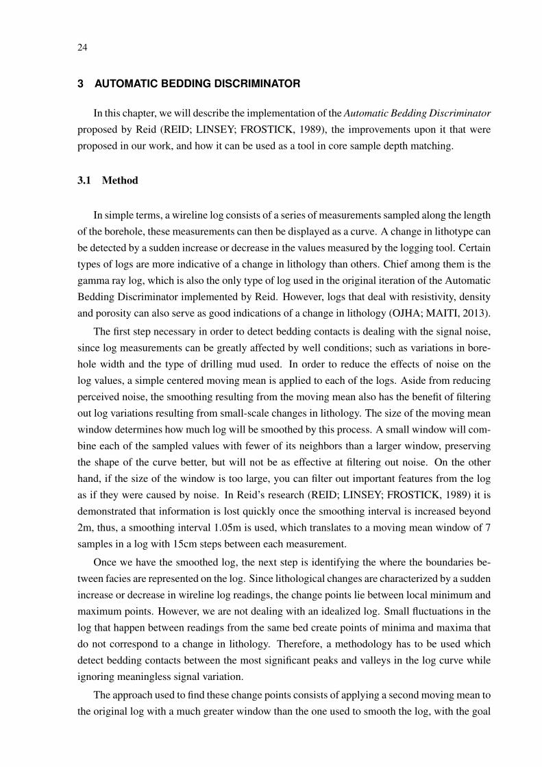
The approach used to find these change points consists of applying a second moving mean tothe original log with a much greater window than the one used to smooth the log, with the goal

25

of extracting a curve that shows the general trend of the log. We can then determine the locationsof the bedding contacts by identifying at which depths this curve intersects the smoothed log.As with the log smoothing operation, the size of the long smoothing window is also an importantparameter in determining the sensitivity of the algorithm’s detection: windows that are too shortwill tend to recognize noise as legitimate bedding contacts, and windows that are too long willignore important signal variations. As extreme examples, we have a long window that is thesame length as the short window, both curves will be the same, and thus, intersect at every point.We can also have a long window that covers the entire length of the log, which will create aflat line that will intersect with the smoothed log only when it crosses the average value of thewhole log. Reid’s research suggests that an interval of 10m be used for the long window. In thiswork, we will call the size of the short window ws, and the size of the long window wl.

Figure 3.1: Example of moving means being used to detect change points in an arbitrary dataset.Filter 1 is obtained by applying a small moving window to the original data, Filter 2 by apply-ing a larger one. The final result displayed is obtained by averaging all values between eachintersection. Source (MACDOUGALL; NANDI, 1997)

Since this method works based on relative differences between log values, special consid-eration must also be made in cases where the log in question is monotonous, showing littledifference between absolute log values along a considerable depth, most likely this means a

26

large depth consisting of the same lithology. In these cases, we can establish a threshold andtell the algorithm to ignore intersections resulting from changes in value that don’t exceed thisthreshold. Reid’s original implementation (REID; LINSEY; FROSTICK, 1989) focuses exclu-sively in the application of this method to gamma ray logs, and uses a threshold of 4 API todemarcate bedding planes. We will call this threshold the noise threshold, or nt.

In this work, we decided to apply Reid’s method not only to gamma ray logs, but to createa generic application that can take any number of logs from the same well as input, applythe Automatic Bedding Discriminator described in Reid’s paper to each one of them and thencorroborate bedding contact evidence across multiple logs for a more accurate assessment.

It is important to keep in mind that wireline logs have different degrees of representative-ness when it comes to lithology. Logs measuring gamma ray emissions can tell the amount oforganic content in the rock and differentiate between shale and sandstone. Porosity is also animportant lithological factor, so logs that are used to infer density, such as sonic and neutronlogs are also strongly tied to lithological characteristics. Resistivity logs are also used as anindication of lithology, but often to a lesser degree compared to the logs previously discussed(KRYGOWSKI, 2003).

LAS files also come with logs that have little to no lithological significance, the caliper logfor instance, that measures the width of the borehole can provide important information to theengineering crew tasked with developing the well. While it is true that a friable rock crackmore easily during drilling, leading to a larger borehole size, the caliper log is still not a reliablelithological marker. We also have logs related to the logging process on a LAS file, such astool tension and transit time, which are used by the logging company to correct and compensatemeasurements from other logs.

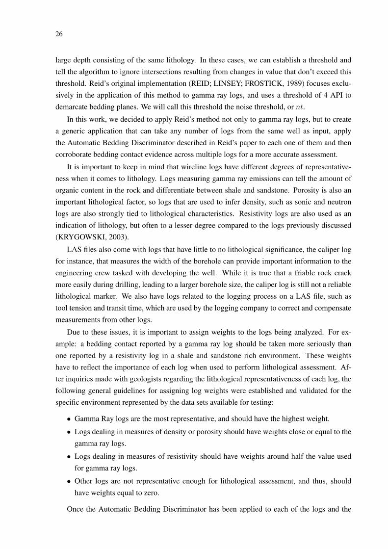
Due to these issues, it is important to assign weights to the logs being analyzed. For ex-ample: a bedding contact reported by a gamma ray log should be taken more seriously thanone reported by a resistivity log in a shale and sandstone rich environment. These weightshave to reflect the importance of each log when used to perform lithological assessment. Af-ter inquiries made with geologists regarding the lithological representativeness of each log, thefollowing general guidelines for assigning log weights were established and validated for thespecific environment represented by the data sets available for testing:

• Gamma Ray logs are the most representative, and should have the highest weight.

• Logs dealing in measures of density or porosity should have weights close or equal to thegamma ray logs.

• Logs dealing in measures of resistivity should have weights around half the value usedfor gamma ray logs.

• Other logs are not representative enough for lithological assessment, and thus, shouldhave weights equal to zero.

Once the Automatic Bedding Discriminator has been applied to each of the logs and the

27

weights have been assigned, we can integrate these separate results into a unified assessment ofbedding contacts. This is done by going through each sampled depth and verifying how manylogs accuse a break at that depth; if the sum of the value of the weights of those logs is equal orgreater than a user-defined threshold, that depth is declared as a bedding contact. This thresholdwill be referred in this work as the agreement threshold, or at.

3.2 Implementation

In this section, I will detail the algorithm employed to implement the method described inthe last section. First, we will take a look at the files and data structures used to store the databeing analyzed.

3.2.1 Loading Data Structures

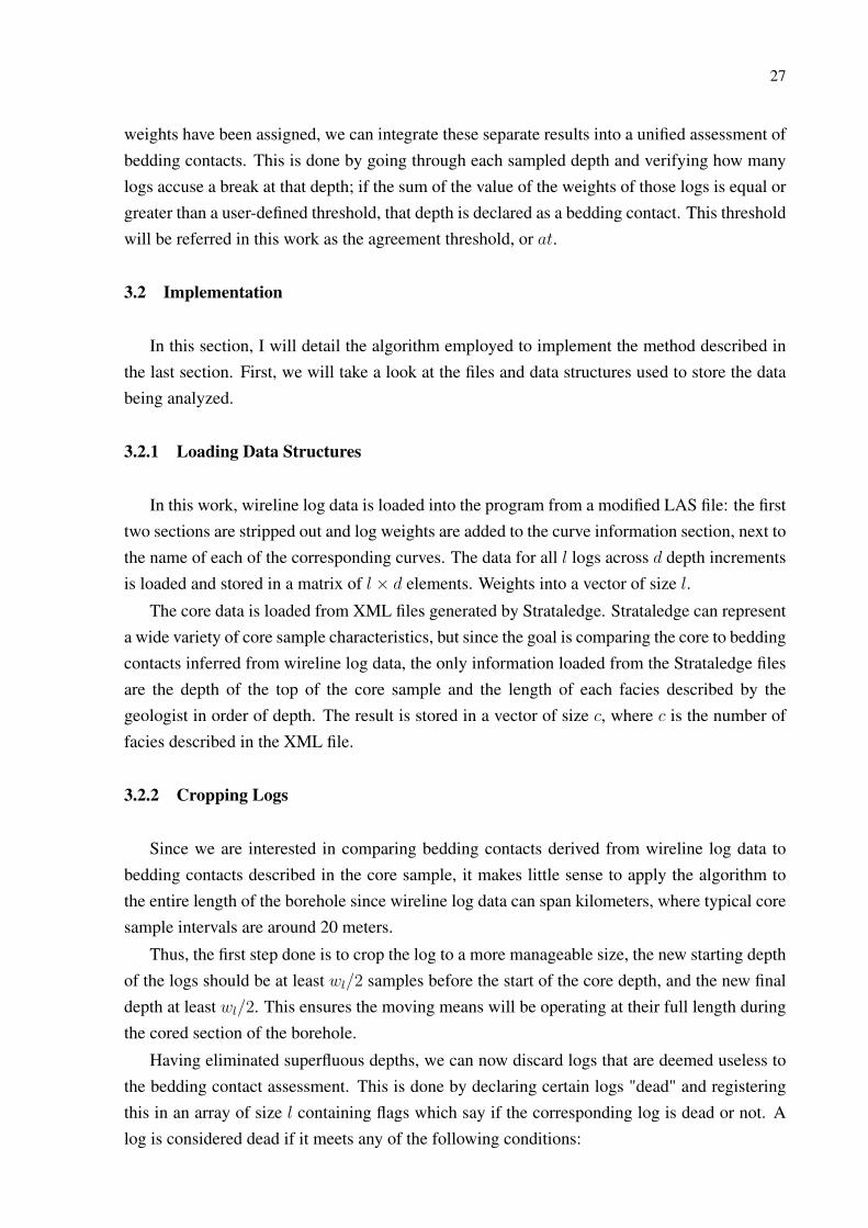
In this work, wireline log data is loaded into the program from a modified LAS file: the firsttwo sections are stripped out and log weights are added to the curve information section, next tothe name of each of the corresponding curves. The data for all l logs across d depth incrementsis loaded and stored in a matrix of l × d elements. Weights into a vector of size l.

The core data is loaded from XML files generated by Strataledge. Strataledge can representa wide variety of core sample characteristics, but since the goal is comparing the core to beddingcontacts inferred from wireline log data, the only information loaded from the Strataledge filesare the depth of the top of the core sample and the length of each facies described by thegeologist in order of depth. The result is stored in a vector of size c, where c is the number offacies described in the XML file.

3.2.2 Cropping Logs

Since we are interested in comparing bedding contacts derived from wireline log data tobedding contacts described in the core sample, it makes little sense to apply the algorithm tothe entire length of the borehole since wireline log data can span kilometers, where typical coresample intervals are around 20 meters.

Thus, the first step done is to crop the log to a more manageable size, the new starting depthof the logs should be at least wl/2 samples before the start of the core depth, and the new finaldepth at least wl/2. This ensures the moving means will be operating at their full length duringthe cored section of the borehole.

Having eliminated superfluous depths, we can now discard logs that are deemed useless tothe bedding contact assessment. This is done by declaring certain logs "dead" and registeringthis in an array of size l containing flags which say if the corresponding log is dead or not. Alog is considered dead if it meets any of the following conditions:

28

1. Its assigned weight is zero.

2. More than 20% of its values are null.

A dead log is ignored by the rest of the algorithm, but can still be displayed in the interfaceat the discretion of the user. The length of the cropped logs will be referred to as dc, note thatthe logs declared dead are not discarded, but simply considered inactive, so, the first dimensionof the matrix storing the cropped log remains the same, resulting in a matrix of l × dc.

During this operation, we also calculate the noise thresholds of each log by finding thehighest and lowest non-null values on the log and multiplying the difference between thosemeasurements by a value between 0 and 1. This value can be changed in the program interface.

Naturally, if the user desires to use the application to detect bedding contacts across thewhole length of the borehole, the depth cropping step of this section can be skipped, and thecomplete log be used in place of its cropped version in the rest of the application. In this case,the rule regarding declaring logs dead if it contains too many null values should be rescinded,since every log will be relevant at some point in the well.

3.2.3 Moving Means

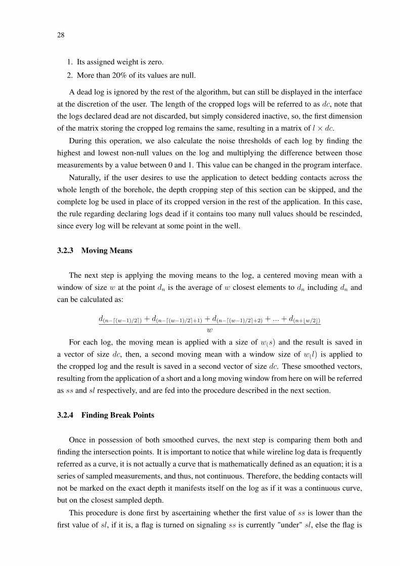
The next step is applying the moving means to the log, a centered moving mean with awindow of size w at the point dn is the average of w closest elements to dn including dn andcan be calculated as:

d(n−d(w−1)/2e) + d(n−d(w−1)/2e+1) + d(n−d(w−1)/2e+2) + ...+ d(n+bw/2c)

w

For each log, the moving mean is applied with a size of w(s) and the result is saved ina vector of size dc, then, a second moving mean with a window size of w(l) is applied tothe cropped log and the result is saved in a second vector of size dc. These smoothed vectors,resulting from the application of a short and a long moving window from here on will be referredas ss and sl respectively, and are fed into the procedure described in the next section.

3.2.4 Finding Break Points

Once in possession of both smoothed curves, the next step is comparing them both andfinding the intersection points. It is important to notice that while wireline log data is frequentlyreferred as a curve, it is not actually a curve that is mathematically defined as an equation; it is aseries of sampled measurements, and thus, not continuous. Therefore, the bedding contacts willnot be marked on the exact depth it manifests itself on the log as if it was a continuous curve,but on the closest sampled depth.

This procedure is done first by ascertaining whether the first value of ss is lower than thefirst value of sl, if it is, a flag is turned on signaling ss is currently "under" sl, else the flag is

29

turned off. Additionally, if the first value of ss is equal to the first value of sl, a bedding contactis marked on the first position.

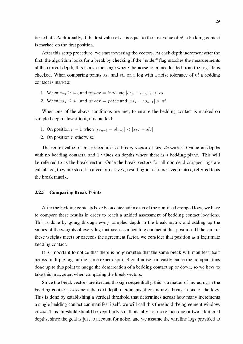
After this setup procedure, we start traversing the vectors. At each depth increment after thefirst, the algorithm looks for a break by checking if the "under" flag matches the measurementsat the current depth, this is also the stage where the noise tolerance loaded from the log file ischecked. When comparing points ssn and sln on a log with a noise tolerance of nt a beddingcontact is marked:

1. When ssn ≥ sln and under = true and |ssn − ssn−1| > nt

2. When ssn ≤ sln and under = false and |ssn − ssn−1| > nt

When one of the above conditions are met, to ensure the bedding contact is marked onsampled depth closest to it, it is marked:

1. On position n− 1 when |ssn−1 − sln−1| < |ssn − sln|2. On position n otherwise

The return value of this procedure is a binary vector of size dc with a 0 value on depthswith no bedding contacts, and 1 values on depths where there is a bedding plane. This willbe referred to as the break vector. Once the break vectors for all non-dead cropped logs arecalculated, they are stored in a vector of size l, resulting in a l × dc sized matrix, referred to asthe break matrix.

3.2.5 Comparing Break Points

After the bedding contacts have been detected in each of the non-dead cropped logs, we haveto compare these results in order to reach a unified assessment of bedding contact locations.This is done by going through every sampled depth in the break matrix and adding up thevalues of the weights of every log that accuses a bedding contact at that position. If the sum ofthese weights meets or exceeds the agreement factor, we consider that position as a legitimatebedding contact.

It is important to notice that there is no guarantee that the same break will manifest itselfacross multiple logs at the same exact depth. Signal noise can easily cause the computationsdone up to this point to nudge the demarcation of a bedding contact up or down, so we have totake this in account when comparing the break vectors.

Since the break vectors are iterated through sequentially, this is a matter of including in thebedding contact assessment the next depth increments after finding a break in one of the logs.This is done by establishing a vertical threshold that determines across how many incrementsa single bedding contact can manifest itself, we will call this threshold the agreement window,or aw. This threshold should be kept fairly small, usually not more than one or two additionaldepths, since the goal is just to account for noise, and we assume the wireline logs provided to

30

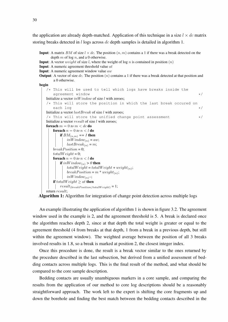
the application are already depth-matched. Application of this technique in a size l× dc matrixstoring breaks detected in l logs across dc depth samples is detailed in algorithm 1.

Input: A matrix BM of size l × dc. The position (n,m) contains a 1 if there was a break detected on thedepth m of log n, and a 0 otherwise.

Input: A vector weight of size l, where the weight of log n is contained in position (n)Input: A numeric agreement threshold value atInput: A numeric agreement window value awOutput: A vector of size dc. The position (n) contains a 1 if there was a break detected at that position and

a 0 otherwise.begin

/* This will be used to tell which logs have breaks inside theagreement window */

Initialize a vector inWindow of size l with zeroes;/* This will store the position in which the last break occured on

each log */Initialize a vector lastBreak of size l with zeroes;/* This will store the unified change point assessment */Initialize a vector result of size l with zeroes;foreach m = 0 to m < dc do

foreach n = 0 to n < l doif BM(n,m) == 1 then

inWindow(n) = aw;lastBreak(n) = m;

breakPosition = 0;totalWeight = 0;foreach n = 0 to n < l do

if inWindow(n) > 0 thentotalWeight = totalWeight + weight(n);breakPosition = m * weight(n);inWindow(n)–;

if totalWeight ≥ at thenresult(breakPosition/totalWeight) = 1;

return result;Algorithm 1: Algorithm for integration of change point detection across multiple logs

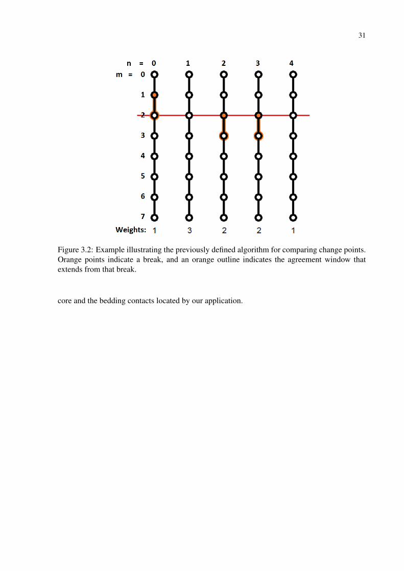
An example illustrating the application of algorithm 1 is shown in figure 3.2. The agreementwindow used in the example is 2, and the agreement threshold is 5. A break is declared oncethe algorithm reaches depth 2, since at that depth the total weight is greater or equal to theagreement threshold (4 from breaks at that depth, 1 from a break in a previous depth, but stillwithin the agreement window). The weighted average between the position of all 3 breaksinvolved results in 1.8, so a break is marked at position 2, the closest integer index.

Once this procedure is done, the result is a break vector similar to the ones returned bythe procedure described in the last subsection, but derived from a unified assessment of bed-ding contacts across multiple logs. This is the final result of the method, and what should becompared to the core sample description.

Bedding contacts are usually unambiguous markers in a core sample, and comparing theresults from the application of our method to core log descriptions should be a reasonablystraightforward approach. The work left to the expert is shifting the core fragments up anddown the borehole and finding the best match between the bedding contacts described in the

31

Figure 3.2: Example illustrating the previously defined algorithm for comparing change points.Orange points indicate a break, and an orange outline indicates the agreement window thatextends from that break.

core and the bedding contacts located by our application.

32

4 RESULTS

In this chapter, I will present the results obtained by applying the bedding detection methodto two sets of wireline log data procured from two wells in the Espirito Santo basin. Thebedding contacts are plotted in yellow, and the core sample beddings are displayed to the right.The cores in these cases have already been depth matched by using core gamma readings asdescribed in 2.2

Unfortunately, the data provided for testing was ill-suited to the task at hand. The carbonatelithology described in the core samples show a high degree of homogeneity and the similarlithotypes translate into monotonous logs, consequently, the noise threshold has to be set to avery low value for any bedding contacts to be detected. A more ideal case would be a coreshowing contrasting lithotypes with distinctive log readings, such as shale and sandstone.

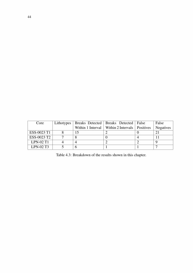
A breakdown of the results obtained from the data provided for testing can be seen in table4.3. This table show how many bedding contacts present on the core were detected in thecore within one and two increments of accuracy. The number of bedding contacts detectedon the logs that were not present on the core sample (false positives), the number of beddingcontacts present on the core not detected in the logs (false negatives) and the number of differentlithotypes present on the core sample. Bedding planes detected outside of the cored interval arenot considered in this calculation. It is also important to know that the intercalation of thinfacies on core ESS-0023 T1 is supposed to be a single conglomerate lithotype. It can be seenthat when detection occurs, it is usually accurate, but due to the similarity between lithotypesin these wells, there is a large number of false negatives, since these similarities translate tominute changes on the log readings.

4.1 Well ESS-0023

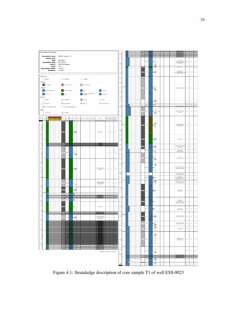
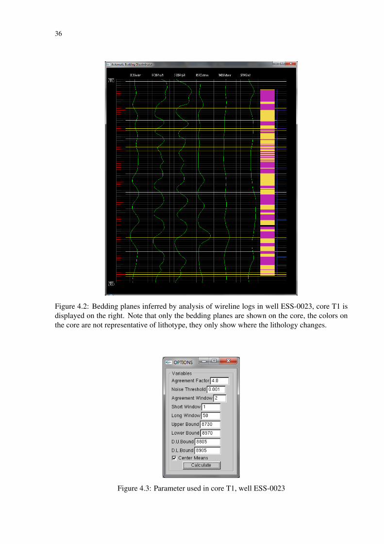
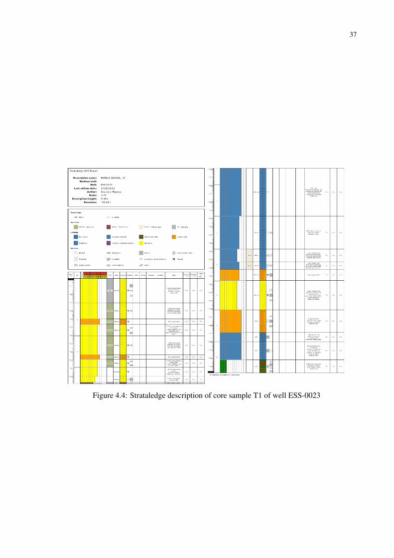
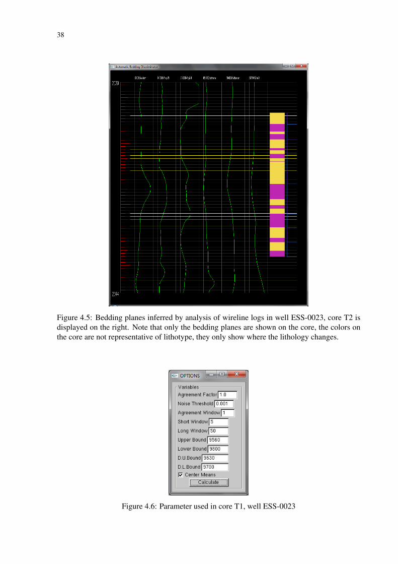
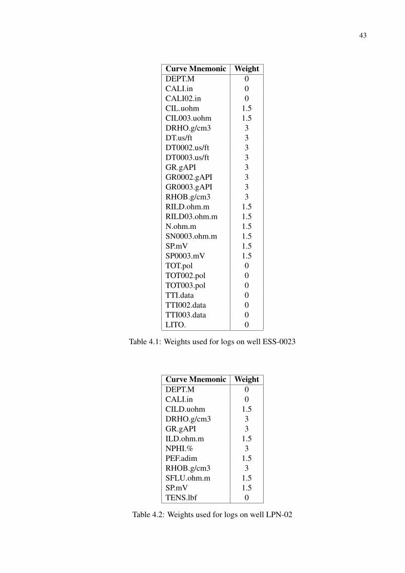
Well ESS-0023 is an offshore well located in the Espirito Santo basin approximately 6 kilo-meters away from the shore. Wireline log data from this well is taken in steps of 20 centimetersand has been described by an inquired expert as of poor quality. A total of 26 curves are presenton the LAS file, however, most of them are null for large lengths of data, indicating they are orig-inated from multiple logging runs done at different depths. Cores T1 and T2 were redescribedin Strataledge based on previously made descriptions done by hand. These core descriptionscan be seen in figures 4.1 and 4.4 respectively. Weights used for the logs in well ESS-0023 areseen in table 4.1. These weights were defined by following the guidelines described in section3.1. The results from the application of the method on cores T1 and T2 are shown in figures 4.2and 4.5, with parameters used in each case shown in figures 4.3 and 4.6.

These were the best results obtained on those cores after experimentation with differentparameters. While a substantial number of bedding contacts described on the log were notdetected, most of the bedding contacts that were detected by the algorithm are marked within

33

less than one or two samples to bedding contacts on the core, especially on core T1. It is alsoof note that when presented with these results, an inquired expert could not detect any beddingcontacts from visual inspection of the logs, while the application did detect bedding contactsthat are confirmed in the core sample description.

4.2 Well LPN-002

Well LPN-002 is located inland, approximately 5 kilometers from the shore in the EspiritoSanto basin. Wireline log data from this well is taken in steps of 15.24 centimeters and havebeen described by an expert as of higher quality than the data from well ESS-0023. Coresamples however, reveal an extremely homogeneous carbonate lithology, which is reflected inthe monotonous lines plotted by the wireline log data. Well LPN-002 has a much shallowerdepth than well ESS-0023, and data from this well is presented in 12 logs, most of which areactive for most of the logged depth, indicating they were likely taken in a single logging run.Cores T1 and T3 can be seen in figures 4.7 and 4.10. Weights used for the logs in well LPN-002 are seen in table 4.2. These weights were defined by following the guidelines described insection 3.1. Results from applying parameters shown in figures 4.9 and 4.12 to cores T1 and T3can be seen in figures 4.8 and 4.11.

Despite the higher quality logging data, results on this well were noticeably worse than onwell ESS-0023, mostly due to the fact that the extremely similar lithotypes make it hard todistinguish bedding contacts. Parameters have to be adjusted in a way as to consider slightvariations as a possible bedding contact, and that causes noise to register as bedding contacts.

4.3 Effects of Parameters in Contact Detection

As expected, changing the parameters can lead to wildly different results. For the carbon-ate lithology present in these wells, parameters that control noise filtering such as the noisethreshold and the size of the short moving mean window had to be kept low in order to detect areasonable number of bedding contacts. The noise threshold in particular had to be kept under0.5% for any detection to be made, this translates to a number much lower than the 4 API noisethreshold used in Reid’s research (REID; LINSEY; FROSTICK, 1989).

Controlling the size of the long moving mean window also allows increasing or decreasingthe detection of bedding contacts. A long window that is close in size to the short windowmakes it easier for the means to intersect, resulting in more detections.

The agreement factors are especially important in increasing detection accuracy in data setswith more monotonous logs. Decreasing the agreement factor needed to declare a break canhelp detection considerably by having logs with lower weights declare breaks without needingcorroboration from other logs, while increasing it can reduce the number of false positives insets with many bedding contacts detected.

34

The agreement window can create a huge number of false positives if used irresponsibly,values greater than two will start showing large sections of the log with multiple consecutivebedding contacts. Increasing it can be useful in cases where that is the behavior that is expectedhowever, such as when the core sample has a series of thin facies.

35

Figure 4.1: Strataledge description of core sample T1 of well ESS-0023

36

Figure 4.2: Bedding planes inferred by analysis of wireline logs in well ESS-0023, core T1 isdisplayed on the right. Note that only the bedding planes are shown on the core, the colors onthe core are not representative of lithotype, they only show where the lithology changes.

Figure 4.3: Parameter used in core T1, well ESS-0023

37

Figure 4.4: Strataledge description of core sample T1 of well ESS-0023

38

Figure 4.5: Bedding planes inferred by analysis of wireline logs in well ESS-0023, core T2 isdisplayed on the right. Note that only the bedding planes are shown on the core, the colors onthe core are not representative of lithotype, they only show where the lithology changes.

Figure 4.6: Parameter used in core T1, well ESS-0023

39

Figure 4.7: Strataledge description of core sample T1 of well LPN-02

40

Figure 4.8: Bedding planes inferred by analysis of wireline logs in well LPN-02, core T1 isdisplayed on the right. Note that only the bedding planes are shown on the core, the colors onthe core are not representative of lithotype, they only show where the lithology changes.

Figure 4.9: Parameter used in core T1, well LPN-02

41

Figure 4.10: Strataledge description of core sample T3 of well LPN-02

42

Figure 4.11: Bedding planes inferred by analysis of wireline logs in well LPN-02, core T3 isdisplayed on the right. Note that only the bedding planes are shown on the core, the colors onthe core are not representative of lithotype, they only show where the lithology changes.

Figure 4.12: Parameter used in core T3, well LPN-02

43

Curve Mnemonic WeightDEPT.M 0CALI.in 0CALI02.in 0CIL.uohm 1.5CIL003.uohm 1.5DRHO.g/cm3 3DT.us/ft 3DT0002.us/ft 3DT0003.us/ft 3GR.gAPI 3GR0002.gAPI 3GR0003.gAPI 3RHOB.g/cm3 3RILD.ohm.m 1.5RILD03.ohm.m 1.5N.ohm.m 1.5SN0003.ohm.m 1.5SP.mV 1.5SP0003.mV 1.5TOT.pol 0TOT002.pol 0TOT003.pol 0TTI.data 0TTI002.data 0TTI003.data 0LITO. 0

Table 4.1: Weights used for logs on well ESS-0023

Curve Mnemonic WeightDEPT.M 0CALI.in 0CILD.uohm 1.5DRHO.g/cm3 3GR.gAPI 3ILD.ohm.m 1.5NPHI.% 3PEF.adim 1.5RHOB.g/cm3 3SFLU.ohm.m 1.5SP.mV 1.5TENS.lbf 0

Table 4.2: Weights used for logs on well LPN-02

44

Core Lithotypes Breaks DetectedWithin 1 Interval

Breaks DetectedWithin 2 Intervals

FalsePositives

FalseNegatives

ESS-0023 T1 8 15 2 0 21ESS-0023 T2 7 8 0 4 11LPN-02 T1 4 4 2 2 9LPN-02 T3 5 6 1 1 7

Table 4.3: Breakdown of the results shown in this chapter.

45

5 CONCLUSION

Despite being based on a method that was proven to provide reliable results, and with im-provements based upon strong theoretical foundations validated by specialists in the field ofgeology, the results of my work proved lacking in providing sufficient information to performcore depth-matching on the data sets that were provided for testing. This can be ascribed to thefact that the data sets used were ill-suited to wireline log analysis; the abundant carbonate rockspresent on the wells used can not be easily distinguished in wireline log data.

However, even in those cases the algorithm is still capable of detecting the more well-definedbedding planes. This information can still be useful to a specialist to perform core depth match-ing assuming the specialist can identify which of the bedding planes described on the coresample are the most obvious and thus, more likely to be detected by the application.

It is also worth noting that in order to achieve these results, it was necessary to experimentwith the parameters until a better fit was reached, in a real situation, where the core was notadjusted, comparing the application output with the core description would be harder, sincethere would be no direct correlation between core and log depths.

Limitations arise with this technique’s high dependence on quality log data, the size of thestep between measurements can have a deep impact on the results. Not only a geological featurethinner than the step size can be skipped over by the measuring tool, accuracy suffers due tothe fact that breaks can only be marked on the sampled depths, when most likely, they occurbetween them. Interpolating points between sampled depths can help with the latter problem,but not with the former.

It is also of note that the method does not look specifically for lithology changes, but for anyheterogeneity. While the most common heterogeneities will be changes in lithology, they canalso be caused by other features, such as presence of fluid in the rock formation or diagenesis.This is still useful information however, as these features can be identified in the core sample.

Enhancements to the method can be made, such as varying the parameters dynamicallybased on the nearest data; for example, it can be a good idea to lower the noise threshold in aparticular monotonous section of the log or decrease the size of the short moving means windowon a section where many thin facies are suspected. It can also be an interesting idea to analyzethe core sample data and adjust the parameters in a way that the application finds facies ofthickness similar to the ones described on the core.

A procedure to adjust the core depth based on bedding plane assessment automatically canalso be developed, but viability and accuracy would be highly dependent on results from thebedding plane assessment.

In conclusion, while the method is sound and shows some promise, more extensive testingwith better datasets is required in order to prove its viability. Validation must also be made withspecialists in order to verify whether or not the results are useful for the task of core depth-matching, and how accurate is matching done with this data.

46

REFERENCES

BRERETON, N.; GALLOIS, R.; WHITTAKER, A. Enhanced lithological description of aJurassic mudrock sequence using geophysical wireline logs. Petroleum Geoscience, [S.l.],v.7, n.3, p.315–320, 2001.

CRANGLE, R. D. Log ASCII Standard(LAS) Files for Geophysical Wireline Well Logs andTheir Application to Geologic Cross Sections through the Central Appalachian Basin. Open-file Report. U. S. Geological Survey, [S.l.], p.14, 2007.

DURANTI, D. et al. Injected and remobilized Eocene sandstones from the Alba Field, UKCS:core and wireline log characteristics. Petroleum Geoscience, [S.l.], v.8, n.2, p.99–107, 2002.

FLEMINGS, P.; BEHRMANN, J. H.; JOHN, C. Gulf of Mexico Hydrogeology (Expeditions308 of the riserless drilling platform from Mobile, Alabama, to Balboa, Panama, Sites U1319-U1324). Proceedings of the Integrated Ocean Drilling Program: Scientific Results, [S.l.],v.308, p.1–70, 2006.

FONTANA, E.; ITURRINO, G. J.; TARTAROTTI, P. Depth-shifting and orientation of coredata using a core–log integration approach: a case study from odp–iodp hole 1256d. Tectono-physics, [S.l.], v.494, n.1, p.85–100, 2010.

GIFFORD, C. M.; AGAH, A. Collaborative multi-agent rock facies classification from wirelinewell log data. Engineering Applications of Artificial Intelligence, [S.l.], v.23, n.7, p.1158–1172, 2010.

HYNE, N. J. Nontechnical guide to petroleum geology, exploration, drilling, and produc-tion. [S.l.]: PennWell Books, 2012.

KRYGOWSKI, D. A. Guide to petrophysical Interpretation. Austin Texas USA, [S.l.], 2003.

LOFTS, J. C.; BRISTOW, J. Aspects of core-log integration: an approach using high resolutionimages. Geological Society, London, Special Publications, [S.l.], v.136, n.1, p.273–283,1998.

MACDOUGALL, S.; NANDI, A. K. Hybrid Bayesian procedures for automatic detection ofchange-points. Journal of the Franklin Institute, [S.l.], v.334, n.4, p.575–597, 1997.

MALINVERNO, A. Well Logging Principles and Applications G9947 - Seminar in MarineGeophysics. 2008.

MANN, U.; LEYTHAEUSER, D.; MÜLLER, P. Relation between source rock properties andwireline log parameters: an example from lower jurassic posidonia shale, nw-germany. Or-ganic geochemistry, [S.l.], v.10, n.4, p.1105–1112, 1986.

47

MORTON-THOMPSON, D.; WOODS, A.; GEOLOGISTS, A. Development Geology Refer-ence Manual: aapg methods in exploration series, no. 10. [S.l.]: American Association ofPetroleum Geologists, 1993. (Methods in Exploration Series).

OJHA, M.; MAITI, S. Sediment classification using neural networks: an example from the site-u1344a of {IODP} expedition 323 in the bering sea. Deep Sea Research Part II: TopicalStudies in Oceanography, [S.l.], n.0, p.–, 2013.

PERRIN, M. et al. Ontology-based rock description and interpretation. Shared Earth Model-ing: Knowledge based solutions for building and managing subsurface structural mod-els., [S.l.], 2012.

REID, I.; LINSEY, T.; FROSTICK, L. E. Automatic bedding discriminator for use with digitalwireline logs. Marine and petroleum geology, [S.l.], v.6, n.4, p.364–369, 1989.

SIDDIQUI, S. Method for depth-matching using computerized tomography. US Patent6,876,721.

VINEGAR, H. J.; WELLINGTON, S. L. Method of correlating a core sample with its origi-nal position in a borehole. US Patent 4,542,648.

WORTHINGTON, P. F. et al. Reservoir characterization at the mesoscopic scale. ReservoirCharacterization II, [S.l.], p.123–165, 1991.