behavior and analysis of plattforms building system
TRANSCRIPT

BEHAVIOR AND ANALYSIS OF PLATTFORMS
BUILDING SYSTEM
by
Bret Albert Burkhart
A thesis submitted to the faculty of The University of Utah
in partial fulfillment of the requirements for the degree of
Master of Science
Department of Civil and Environmental Engineering
University of Utah
December 2011

Copyright © Bret Albert Burkhart 2011
All Rights Reserved

STATEMENT OF THESIS APPROVAL
The thesis of Bret Albert Burkhart
has been approved by the following supervisory committee members:
Chris Pantelides , Chair 12/15/2010
Date Approved
Lawrence Reaveley , Member 12/15/2010
Date Approved
Paul Tikalsky , Member 12/15/2010
Date Approved
and by Paul Tikalsky , Chair of
the Department of Civil and Environmental Engineering

ABSTRACT A new structural building system (Plattforms) was investigated at the University
of Utah. The system was analyzed to determine capacity, behavior, and residual strength.
Three short span specimens of the system were tested to failure. This thesis addresses the
layout of the test specimens as well as their performance under gravity type loading up to
ultimate conditions. The thesis also presents a strut and tie method of analysis that may
be useful in the development and design of current and new versions of the plattforms
building system. The building system offers a prefabricated product to compete with the
conventional concrete deck over steel beam floor systems available for construction and
design.

TABLE OF CONTENTS
ABSTRACT ....................................................................................................................... iii
LIST OF FIGURES ........................................................................................................... vi
LIST OF TABLES ............................................................................................................ vii
ACKNOWLEDGMENTS ............................................................................................... viii
CHAPTERS
1. INTRODUCTION ...........................................................................................................1
2. SCOPE AND OBJECTIVES ...........................................................................................4
3. TESTING PROGRAM ....................................................................................................5
3.1 Test Specimens .......................................................................................................... 5
3.2 Instrumentation .......................................................................................................... 5
3.3 Loading Regime ........................................................................................................ 8
4. EXPERIMENTAL RESULTS.......................................................................................12
4.1 Load vs. Deflection ................................................................................................. 12
4.2 Displaced Shape ...................................................................................................... 14
4.3 Location of Neutral Axis…………………………………………………………..14
5. ANALYTICAL RESULTS ...........................................................................................18
5.1 Flexural Analysis ..................................................................................................... 18
5.2 Theoretical Flexural Analysis ................................................................................. 18
5.3 Shear Analysis ......................................................................................................... 24
5.4 Theoretical Shear Analysis ...................................................................................... 24

v
6. COMPOSITE BEHAVIOR ...........................................................................................27
6.1 Strut and Tie Model ................................................................................................. 27
6.2 Numerical Results of Strut and Tie Model .............................................................. 30
6.3 Observed Strut and Tie Formation .......................................................................... 31
7. DISCUSSION OF EXPERIMENTAL AND ANALYTICAL RESUTS ......................34
8. CONCLUSIONS............................................................................................................37
APPENDIX: STRUT AND TIE MODEL CALCULATIONS .........................................40
REFERENCES ..................................................................................................................44
LIST OF FIGURES Figure Page 3.1: Specimen Layout ......................................................................................................... 6
3.2: Instrumentation ............................................................................................................ 7
3.3: Specimen 1 Loading .................................................................................................. 10
3.4: Specimen 2 and 3 Loading......................................................................................... 11
4.1: Load vs. Displacement Comparison .......................................................................... 13
4.2: Specimen III Displaced Shape ................................................................................... 15
4.3 Picture of Displaced Shape ......................................................................................... 15
4.4: Location of Neutral Axis Plots and Horizontal Strain at Midspan: (a) SPM I, (b) SPM II, and (c) SPM III .................................................................................................... 16 5.1: Moment Diagrams: (a) SPM I, (b) SPM II, (c) SPM III ............................................ 19
5.2: Theoretical Stress Distribution .................................................................................. 23
5.3: Theoretical Shear Diagrams: (a) SPM I, (b) SPM II, (c) SPM III ............................. 25
6.1:Three Dimentional Strut and Tie Load Paths ............................................................. 28
6.2: Geometric Requirements for Strut and Tie Model .................................................... 28
6.3: Typical Cracking of End Stem Wall .......................................................................... 33
6.4: Cracking of Center Stem Wall SPM II ...................................................................... 33

LIST OF TABLES Table Page
5-1: Tensile Force in Steel Beam Based on Observed Strains.......................................... 21
5-2: Compressive Force in Steel Beam Based on Observed Strains ................................ 23
6-1: Forces Summary ........................................................................................................ 31
7-1: Summary Results ....................................................................................................... 34
7-2: Observed Capacities .................................................................................................. 35

ACKNOWLEDGMENTS
First and foremost, I would like to thank my advisor, Dr. Chris P. Pantelides. His
expertise, guidance, and encouragement have been instrumental in the completion of this
thesis along with the research work involved therein. I would also like to thank my
faculty committee members Dr. Lawrence D. Reaveley and Dr. Paul Tikalsky for their
further guidance and support.
I also thank my wife, Angela, for her continued support and patience throughout
my academic career.
Funding for this project was provided by Plattforms Inc., of Salt Lake City Utah.
The design of the test specimens were also provided by Plattforms. Special Thanks To:
David Platt, the inventor of the Plattforms system. Darrell Hodgson, head of
manufacturing; as well as, Clayton Burningham, and Mark Bryant for their help in the
testing lab at the University of Utah.

CHAPTER 1
INTRODUCTION
The Plattforms Building System was tested at the Structures Laboratory of the
University of Utah for evaluation of its performance in January 2010. The system is
comparable to the three variants of the traditional floor beam system, which have been
developed over the years to meet height limitations and the need for complex mechanical
installations: composite beams with web openings in the steel beam, composite joists and
trusses and stub girders (Viest, 2.5-2.20). The present system consists of a concrete T-
section with mechanical blockouts connected to a steel beam at the bottom, where the
concrete T-section is connected to a steel beam by nelson studs and welded reinforcing
bars.
The typical test specimens were short span versions of the system with lengths of
13 ft-0 in., widths of 4 ft-0 in., and total heights, including the steel beam, of 2 ft-8 in.
Mechanical blockouts for the test specimens measured 2 ft-4 in. in width and 1 ft-3 3/8in.
in height. A clear image of the layout can be seen in Figure 3.1. Three of these specimens
were tested for this evaluation under four-point loading. All of the specimens can be
classified as short shear spans with a/d ratios of 2.0 for the first specimen and 1.8 for both
the second and third specimens. For code comparison the total load applied to the
specimens was related to the effect of a distributed load on the system. This was done by

2
simply dividing the total load by the area of the deck, and comparing it to ASCE 7
expected live loads for different applications. The worst case loading outlined in ASCE 7
consists of a distributed live load of 250 psf for heavy manufacturing or heavy storage
warehouse applications. Using the equivalent effect of a distributed live load of 250 psf
over the entire surface of the system, and a load factor of 1.6, the following is concluded:
(1) the maximum live load condition falls well within the elastic portion of behavior of
the system. At the point of nonlinearity on the load versus displacement curve, the system
achieved a capacity of 4.3, 4.9, and 5.1 times the factored surface load, where the
variability comes from the two different loading conditions; (2) the displacement at the
maximum live load condition was compared to the maximum permissible deflections in
ACI 318 for the three specimens. It was found to reach only 15% of the allowable for
floors supporting nonstructural elements not likely to be damaged by large deflections to
30% of the allowable for floors supporting nonstructural elements likely to be damaged
by large deflections. The system proved to be very ductile; at the yield condition the three
specimens achieved a displacement of 5.7, 7.7, and 7.8 times the deflection measured at
the maximum live load condition. Failure of the specimens was a shear compression
failure (web shear) which occurred in the 4 in. thick web of the concrete T-sections; this
occurred at an ultimate displacement of 10.8, 11.0, and 11.8 times the deflection
measured at the maximum live load condition; after this ultimate displacement was
reached, the load dropped by 25%, 29%, and 32% of its ultimate value.
The system shows promise for use in the modular prefabricated area of
commercial construction. It has the potential to cut construction time, reduce the quantity

3
of materials used, and provide a cost effective solution for structural frames. This thesis
outlines the results and analysis of the testing performed at the structures lab.

CHAPTER 2
SCOPE AND OBJECTIVES
This thesis consisted of the following research objectives:
1. Test the Plattform Building System specimens to failure to determine their elastic
and ultimate capacity under gravity type loading conditions, as well as measure
associated deflections.
2. Determine the code level of performance of the system.
3. Explore the appropriateness of analyzing the specimens using basic beam theory.
4. Develop a strut and tie model that predicts the behavior of the system and
accounts for the large voids in the beam’s web.
5. Determine the ability of the specimens to act as composite beams, and
recommend potential design improvements

CHAPTER 3
TESTING PROGRAM
3.1 Test Specimens
The Plattforms test specimens were composed of a concrete T-section with
mechanical openings cast onto a W10X12 with nelson studs and reinforcing bars welded
to the top flange. The dimensions and connection layout can be seen in Figure 3.1.
Supports for the testing were 6 in. wide tube steel. Concrete for the specimens consisted
of light weight concrete with compressive strength on the day of the test of: ��� �4950�. A 4X4-W2.0XW2.0 welded wire mesh was cast into the deck, all other
reinforcing bars were #4. The overall dimensions of the specimens were as follows:
length 13 ft., width 4 ft., and depth 2 ft-8 in. Bent plate steel, ¼ in. thick, was cast into the
sides of the deck and reinforced with welded #4 bars and 2 in. nelson studs. Under
normal conditions these plates would be used to attach double T spans to adjacent spans
through welded connections. The steel used for the W10X12 was A992 steel with AISC
code values for yield strength of � �50-65ksi, and ultimate strength of �� � 65��.
3.2 Instrumentation
Each specimen was instrumented slightly differently, with additional strain
gauges and LVDTs being applied as testing progressed. The final layout for strain gauges

6
Figure 3.1: Specimen Layout

7
and LVDTs is shown in Figure 3.2. Strain gauges were used to measure micro strains at
various locations on the steel beam, concrete web, and deck. LVDTs measured deflection
at the bottom of the steel beam.
The first specimen was equipped with strain gauges 1-5, and 7-9, as well as
LVDT 1 at the midspan of the beam. Strain gauges 1-4 were placed to measure strains
resulting from shearing stresses near the support. Strain gauges 5 and 7 measured the
strains resulting from flexure in the I-beams top and bottom flange respectively. LVDT 1
measured downward deflections at the midspan of the beam.
Figure 3.2: Instrumentation

8
The second specimen included all of the strain gauges and LVDTs as the first,
with the addition of strain gauges 6, ll, and 12. It was observed in the first specimen that
the top flange of the steel beam entered into compression while the bottom flange was in
tension. This indicates that the steel beam was carrying load as a flexural member as
opposed to a tension member in a fully composite system. Strain gauge 6 was added to
gather more information regarding the location of the neutral axis of the system. Initial
cracking of the first specimen occurred near strain gauge 11 and 12. These gauges were
added to give insight into the web shear in the concrete end stem walls. LVDTs 2 and 3
were added to help graphically visualize the deflected shape of the beam with greater
detail.
The third specimen included all of the previous strain gauges and LVDTs with the
addition of strain gauges 10 and 13. Previous observation showed consistent failure in the
end stem walls. Gauges 10 and 13 were added to further investigate the strain distribution
that existed in the stem walls.
3.3 Loading Regime
Loading for all specimens was deflection controlled not exceeding 1/16 in. per
minute. Load was transferred from a hydraulic piston to stiffened short span W-sections
and then onto two 2 in. thick steel plates, 8 in. wide by 14 in. long, resting on the deck of
the specimen. The loading pattern was designed to simulate the effects of a distributed
load on the system. At the onset of loading, bending of the specimens resulted in load
transfer to the outer steel plates only (thus for the first test the center plate did not serve
any purpose in distributing load to the system). After the first test it was noted that

9
eccentric loading of the interior stem walls caused flexural cracks in the concrete web.
This result was undesirable as it did not represent the effects of a symmetrically
distributed load. Subsequent tests spread the load such that the load transferring steel
plates were centered above the interior stem walls. A schematic drawing for the loading
regime of the first specimen can be seen in Figure 3.3.
Loading for specimens 2 and 3 was identical to specimen 1, except that the load
was applied closer to the center of the interior stem walls. Eccentricity, e, measured from
the center of the interior stem walls to the application of the load was reduced from 7 in.
to 1 ½ in. for the second and third tests in comparison to the first; this assumes the load
can be approximated as a point load applied at either end of the stiffened loading beam. A
schematic drawing for the loading regime of the second and third specimens can be seen
in Figure 3.4.
The a/d ratio for the test specimens were 2.0 for the first test, and 1.8 for the
second and third tests and can therefore be classified as short shear spans. Short shear
spans are characterized by a/d ratios ranging from 1 to 2.5. During extreme loading they
develop inclined cracks and, after a redistribution of internal forces, are able to carry
additional load in part by arch action. The failure of such beams is generally caused by a
bond failure, a splitting failure, a dowel failure along the tension reinforcement, or -as
was observed in this case- a shear compression failure. Shear compression failures are
characterized by crushing of the compression zone over the top of inclined shear cracks.
Because the inclined crack generally extends higher into the beam than does a flexural
crack, failure occurs at less than the flexural moment capacity (Wight & Macgregor 240).

10
NORTH ELEVATION
EAST ELEVATION
Figure 3.3: Specimen 1 Loading

11
NORTH ELEVATION
EAST ELEVATION
Figure 3.4: Specimen 2 and 3 Loading
CHAPTER 4
EXPERIMENTAL RESULTS
4.1 Load vs. Deflection
For code comparison the total load applied to the specimens was related to the
effect of a distributed load on the system. This was done by simply dividing the total load
by the area of the deck, and comparing it to ASCE 7 expected live loads for different
applications. The worst case loading outlined in ASCE 7 consists of a distributed live
load of 250 psf for heavy manufacturing or heavy storage warehouse applications. Using
the equivalent effect of a distributed live load of 250 psf over the entire surface of the
system, and a load factor of 1.6, the following is concluded: (1) the live load condition
for heavy manufacturing or heavy storage warehouse applications falls well within the
elastic portion of behavior of the system. At the point of nonlinear behavior of the tested
spans, the system achieved a capacity of 4.3, 4.9, and 5.1 times the factored surface load,
where the variability comes from the two different loading conditions; (2) the
displacement at midspan was compared to the maximum permissible deflections in ACI
318 for the three specimens. It was found to reach only 15% of the allowable for floors
supporting nonstructural elements not likely to be damaged by large deflections (L/240)
to 30% of the allowable for floors supporting nonstructural elements likely to be
damaged by large deflections (L/480).

13
At the point of nonlinearity the three specimens achieved a displacement of 5.7,
7.7, and 7.8 times the deflection measured at the factored surface load. Failure of the
specimens was a shear compression failure (web shear) which occurred in the 4 in. thick
web of the concrete T-sections; this occurred at an ultimate displacement of 10.8, 11.0,
and 11.8 times the deflection measured at the factored surface load; immediately after
this ultimate displacement was reached, the load dropped by 25%, 29%, and 32% of its
ultimate value as seen in Figure 4.1.
Figure 4.1: Load vs. Displacement Comparison
-20
0
20
40
60
80
100
120
-0.5 0 0.5 1 1.5 2 2.5
To
tal
Loa
d (
kip
s)
Displacement at Midspan (in.)
LOAD VS DISPLACEMENT COMPARISON
SPM I
SPM II
SPM III
L/180
L/240
L/360
heavy manufacturing live load condition:
250psf x 1.6 x area of deck = 20.8 kips
SPM I point of nonlinearity: 89.1 KIP
SPM III point of nonlinearity: 102.6 KIP
SPM I I point of nonlinearity: 105.9 KIP
14
4.2 Displaced Shape
The curves representing the measured displacement along the member, shown in
Figure 4.2, provide insight to what the moment diagram for the system looks like. The
shape drawn by three points along the base of the beam demonstrate the stiffening effect
that the end stem walls have in restraining the moment. This can also be seen in Figure
4.3. For a simply supported beam we would generally expect a more parabolic shape. The
deflection increases slowly at first with substantial load increase, then progresses rapidly
beyond the ultimate load condition. The final deflection is representative of the system
after a 30% decrease in load compared to the ultimate load condition.
4.3 Location of Neutral Axis
The location of the neutral axis for each specimen was estimated based on strain
compatibility for the yield and ultimate conditions. The neutral axis was estimated as the
distance from the bottom flange where a line joining strain crosses the vertical axis as
shown in Figure 4.4. The location of the neutral axis was estimated at 6.83 in., 7.79 in.,
and 7.64 in. for the first second and third specimens, respectively. The location for the
first specimen likely varies from the other two because of the different loading
conditions.
Tests two and three included an additional strain gauge at the mid-height of the
steel web. The additional gauge provides further information for estimating the location
of the neutral axis. It should also be noted that the low tensile strain at the ultimate load
of specimen II is likely the result of a strain gage malfunction, in which the strain gage

Figure
Figure 4.
-1.6
-1.4
-1.2
-1
-0.8
-0.6
-0.4
-0.2
0
0 20
Dis
pla
cem
en
t (i
n.)
Figure 4.2: Specimen III Displaced Shape
Figure 4.3 Picture of Displaced Shape
40 60 80Distance from Support (in.)
CenterLine
15
5kip
23kip
55kip
90kip
103kip
final
Center

16
Figure 4.4: Location of Neutral Axis Plots and Horizontal Strain at Midspan: (a) SPM I, (b) SPM II, and (c) SPM III
0
5
10
15
20
25
30
35
-0.002 -0.001 0.000 0.001 0.002 0.003
He
igh
t (i
n)
Strain (in./in.)
(a)
Yield
Ultimate
0
5
10
15
20
25
30
35
-0.002 -0.001 0.000 0.001 0.002 0.003
He
igh
t (i
n.)
Strain (in./in.)
(b)
yield
Ultimate
0
5
10
15
20
25
30
35
-0.002 -0.001 0.000 0.001 0.002 0.003
He
igh
t (i
n)
Strain (in./in.)
(c)
yield
ultimate

17
lost adhesion to the bottom surface of the steel beam. However the other three strain
gauges still give a good estimation for the location of the neutral axis of the specimen.
The location of the neutral axis in the web of the steel beam demonstrates that the
specimens never acted as fully composite members. In order for this system to be truly
composite the steel would have to be entirely in tension with the neutral axis located
somewhere in the T-section of the concrete. Instead the test specimens always exhibited
flexural bending in the steel beam. It would be expected that the system would have
higher flexural strength if it were able to perform as a composite member.

CHAPTER 5
ANALYTICAL RESULTS
5.1 Flexural Analysis
For flexural analysis, the theoretical bending moment diagrams at ultimate
loading for each specimen were plotted assuming four-point loading with the forces from
the loading device centered in the middle of the steel load transferring plates as shown in
Figure 5.1. The distance along the x-axis of the moment diagrams represents the span
length from center of support to center of support
5.2 Theoretical Flexural Analysis
The theoretical flexural analysis is limited by because it was observed that the
specimens failed in shear before reaching their flexural moment capacity. The analysis is
therefore based on observed strains from the third test specimen. The third specimen was
chosen because it had more strain gauges at the midspan of the steel beam to measure
longitudinal strains than the first specimen, and unlike the second specimen there were no
issues with possible adhesion loss of strain gauges.
The analysis follows a similar procedure as employed when analyzing a concrete
T-beam with tensile steel reinforcement. The theory for this analysis is based on statics
where forces in a beam are resisted by internal moments, and the largest internal moment

19
Figure 5.1: Moment Diagrams: (a) SPM I, (b) SPM II, (c) SPM III
0500
100015002000250030003500
Mo
me
nt
(kip
-in
.)
Distance (in.)60.75 88.75 149.5
0500
100015002000250030003500
Mo
me
nt
(kip
-in
.)
Distance (in.)54.75 94.75 149.5
0500
100015002000250030003500
Mo
me
nt
(kip
-in
.)
Distance (in.)149.594.7554.75
(a)
(b)
(c)

20
for a simply supported beam under evenly distributed loading will occur at midspan.
Therefore the maximum moment experienced by the beam should equal the tensile force
in the steel multiplied by the distance between the centroid of the tensile and compressive
forces.
It was assumed that the stress block for the concrete was largely rectangular; this
is supported by the nearly vertical slope of the lines between the uppermost strain gauges
in Figure 4.4. The steel mesh in the top deck was not taken into consideration for the
compressive strength of the deck because it was in the compression block. The stress in
the steel is based on the observed strains, where stress equals strain multiplied by the
modulus of steel, except where strains have gone beyond yielding for which stress is
limited to 65ksi. The tensile and compressive forces and centroids of the tensile and
compressive stress distributions were obtained through a weighted area averaging method
using the strains of Figure 4.4, an ultimate stress of 65ksi, and a modulus of steel of
29000ksi. The results of this approach are shown in Table 5-1 and Table 5-2 for tensile
and compressive force distributions respectively.
To summarize Tables 5-1 and 5-2, the height was measured from the base of the
steel beam in the vertical direction. Stress was computed at each height increment using
the strain inferred by Figure 4.4 multiplied by the modulus of steel (29000 ksi). The area
was computed using the dimensions of the steel beam, and the height bounds of the
current and subsequent rows in the tables. The average stress was computed by averaging
the stress from the current and subsequent row. The average force was computed by
multiplying the average stress by the average area. The centroid column was computed as
the center of mass of a trapezoid formed by the strains inferred from Figure 4.4 and

21
Table 5-1: Tensile Force in Steel Beam Based on Observed Strains
height stress area average stress average force centroid force X centroid
(in.) (ksi.) (in.^2) (ksi) (kips) (in) (kip x in.)
0.00 65.00 0.40 65.00 25.74 0.05 1.29
0.10 65.00 0.44 65.00 28.31 0.16 4.39
0.21 65.00 0.20 65.00 12.82 0.32 4.16
0.51 65.00 0.06 65.00 3.71 0.66 2.45
0.81 65.00 0.06 64.89 3.70 0.96 3.55
1.11 64.78 0.06 63.78 3.64 1.26 4.58
1.41 62.78 0.06 61.77 3.52 1.56 5.49
1.71 60.77 0.06 59.76 3.41 1.86 6.33
2.01 58.76 0.06 57.75 3.29 2.16 7.11
2.31 56.75 0.06 55.75 3.18 2.46 7.81
2.61 54.74 0.06 53.74 3.06 2.76 8.45
2.91 52.73 0.06 51.73 2.95 3.06 9.02
3.21 50.73 0.06 49.72 2.83 3.36 9.52
3.51 48.72 0.06 47.71 2.72 3.66 9.95
3.81 46.71 0.06 45.70 2.61 3.96 10.31
4.11 44.70 0.06 43.70 2.49 4.26 10.61
4.41 42.69 0.06 41.69 2.38 4.56 10.83
4.71 40.68 0.06 39.64 2.26 4.86 10.98
5.01 38.60 0.06 36.39 2.07 5.16 10.70
5.31 34.19 0.06 31.98 1.82 5.46 9.95
5.61 29.78 0.06 27.58 1.57 5.76 9.05
5.91 25.37 0.06 23.17 1.32 6.06 8.00
6.21 20.97 0.06 18.76 1.07 6.35 6.80
6.51 16.56 0.06 14.36 0.82 6.65 5.44
6.81 12.15 0.06 9.95 0.57 6.95 3.94
7.11 7.75 0.06 5.54 0.32 7.24 2.29
7.41 3.34 0.06 1.67 0.10 7.51 0.71
7.71 summation 122.26 kips 183.70 kip x in.
centroid 1.50 In.

22
dependent on the distribution of steel area within the bounded heights. The total force
was determined by adding all of the average forces for each area. The centroid was
computed as a weighted average based on the sum of the forces and centroids of each
layer multiplied together, divided by the total force. It was thereby deduced that the total
tensile force developed during testing of the third specimen was 122.26 kips centered 1.5
in. from the base of the steel beam. The compressive force in the steel beam was 38.19
kips centered 9.73 in. up from the steel beam. Figure 5.2 shows the equivalent forces and
centroids graphically. This leaves an unresolved compressive force of 84.07 kips to be
carried by the concrete flange. Knowing the amount of force carried by the concrete
allows us to calculate the depth of the compression zone in the concrete (��.
� � ��������� �������� �����0.85 · ��� · !"
!" # $%�&����� &�!' ( 2 · *8 · +,�� 4⁄ . +, � ��%+ �� ������%� ��&�/�
From the above equations α was calculated as 0.51 in. Assuming the concrete
compressive force acts at the center of the compression block, it is now possible to
determine the resultant compressive force and its line of action. This is done by taking a
weighted average of the compressive forces in the concrete and steel at their lines of
action. The compressive force, adequate to resist the tension in the steel beam, acts at a
centroid 24.87 in. from the base of the beam. This is shown in Figure 5.2. Next the
moment is calculated by multiplying the total tensile force by d, resulting in a moment of
2,857 kip-in. This calculated moment, using strains measured from specimen III, is less
than 1% different from the observed moment of specimen III.

23
Table 5-2: Compressive Force in Steel Beam Based on Observed Strains
height stress area average stress average force centroid force X centroid
(in.) (ksi) (In.^2) (ksi) (kips) (in.) (kip x in.)
10.00 34.71 0.40 33.98 13.45 9.95 133.87
9.90 33.24 0.44 32.43 14.13 9.85 139.09
9.79 31.63 0.20 29.42 5.80 9.68 56.15
9.49 27.22 0.06 25.01 1.43 9.34 13.32
9.19 22.81 0.06 20.61 1.17 9.04 10.62
8.89 18.40 0.06 16.20 0.92 8.74 8.07
8.59 14.00 0.06 11.79 0.67 8.44 5.67
8.29 9.59 0.06 7.39 0.42 8.14 3.43
7.99 5.18 0.06 2.98 0.17 7.84 1.33
7.69 0.78 0.06 0.39 0.02 7.54 0.17
7.39
summation 38.19 kips 371.72 kip x in.
centroid 9.73 In.
Figure 5.2: Theoretical Stress Distribution

24
It is impossible to determine the true moment capacity of the specimens because
they all failed in shear compression. It should be noted that the inability of the system to
achieve full composite action also limits the flexural capacity, because the steel is not
allowed to fully plastify.
5.3 Shear Analysis
The shear analysis assumed the same four-point loading as the flexural analysis
and the shear diagrams for each specimen can be seen in Figure 5.3. Again the span is
taken as the distance from center of support to center of support. The imposed loading is
assumed to be a point load acting at the center of the steel load transfer plate on the
concrete deck.
5.4 Theoretical Shear Analysis
The shear analysis presented in this thesis is focused primarily on the shear
capacity of the concrete web of the test specimens. This is because test observations
showed that this is where shear compression failure occurred. Further, the steel beam has
a code listed shear strength of 012 � 56.3 kips, this is based on fy = 50 ksi and is likely
to be exceeded in actual tests. With reactions measuring in the 50 kip range it is clear that
the steel beam will be capable of carrying the induced shear load, again it is the concrete
web that is of interest. The shear capacity is made up of the shear contribution from the
steel bars and concrete T-section.
The concrete web is not continuous and the mechanical openings in the web are
so large that the entire beam is considered a discontinuity region. For such regions beam

25
Figure 5.3: Theoretical Shear Diagrams: (a) SPM I, (b) SPM II, (c) SPM III
-60
-40
-20
0
20
40
60
Sh
ea
r F
orc
e (
kip
s)
Distance (in)
(a)
60.75 88.75 149.5
-60
-40
-20
0
20
40
60
Sh
ea
r (k
ips)
Distance (in)
(b)
54.75 94.75 149.5
-60
-40
-20
0
20
40
60
she
ar
(kip
s)
Distance (in)
(c)
149.594.7554.75

26
theory does not apply and a method such as a strut and tie model or finite element
analysis should be used to determine the theoretical shear capacity of the specimens. This
thesis presents a strut and tie model in Chapter 6 to analyze the specimens.

CHAPTER 6
COMPOSITE BEHAVIOR St. Venant’s principle indicates that discontinuity occurs in the stress distribution
of a structural element at changes in geometry or at concentrated loads and reactions.
Such discontinuities are typically assumed to extend a distance, h, equal to the overall
height of the member from the section where the load or change in geometry occurs, and
are typically labeled D-regions. In D-regions beam theory does not apply and either
finite-element analysis or a strut-and-tie model is required for analysis (Wight &
Macgregor 841). The Plattforms building system is characterized by large closely spaced
mechanical openings in the concrete web, such that the entire member is classified a D-
region. This thesis applies a simple strut and tie model to the system using idealized
prismatic compression struts in the concrete and steel where applicable.
6.1 Strut and Tie Model
The strut and tie model, for the specimens, consists of prismatic struts, tension
ties, and nodes. Figure 6.1shows the strut and tie load paths based on the location of the
loading plates, reactions, and steel reinforcement in the test specimens. The load paths are
symmetric about a vertical line passing through the specimen midspans. This results in
equal forces being transferred to each of the reactions. Figure 6.2 shows the required

28
PLAN VIEW
ELEVATION VIEW
Figure 6.1:Three Dimentional Strut and Tie Load Paths
PLAN VIEW
ELEVATION VIEW
Figure 6.2: Geometric Requirements for Strut and Tie Model
29
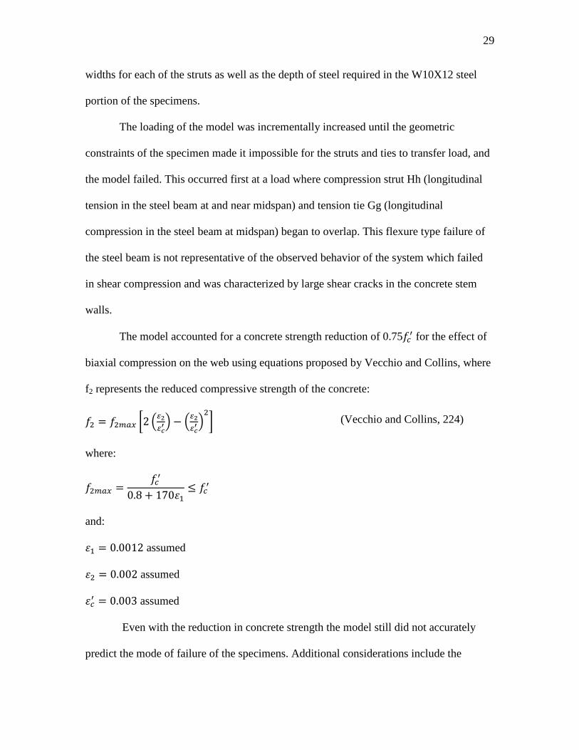
widths for each of the struts as well as the depth of steel required in the W10X12 steel
portion of the specimens.
The loading of the model was incrementally increased until the geometric
constraints of the specimen made it impossible for the struts and ties to transfer load, and
the model failed. This occurred first at a load where compression strut Hh (longitudinal
tension in the steel beam at and near midspan) and tension tie Gg (longitudinal
compression in the steel beam at midspan) began to overlap. This flexure type failure of
the steel beam is not representative of the observed behavior of the system which failed
in shear compression and was characterized by large shear cracks in the concrete stem
walls.
The model accounted for a concrete strength reduction of 0.75��� for the effect of
biaxial compression on the web using equations proposed by Vecchio and Collins, where
f2 represents the reduced compressive strength of the concrete:
�8 � �89:; <2 =>?>@A B C =>?>@A B8D where:
�89:; � ���0.8 ( 170GH # ��� and:
GH � 0.0012 assumed
G8 � 0.002 assumed
G�� � 0.003 assumed
Even with the reduction in concrete strength the model still did not accurately
predict the mode of failure of the specimens. Additional considerations include the
(Vecchio and Collins, 224)

30
assumption that the concrete could support compressive loads along the steep paths
proposed by the model within the stem walls. Had shallower angles, closer to the ideal
45o, been used the model would have failed those compression struts much sooner as they
began to overlap the open space of the mechanical openings. Also per Figure 3.1, some
tensile reinforcement was provided; however to improve the shear capacity of the
specimens would require either a thicker concrete web or increased concrete
confinement. It was also clear in testing that tension tie BC in Figure 6.1 would be more
effective if the vertical reinforcing were placed closer to the mechanical block out.
One of the strengths of this model is the proposed load paths. These show that
under the current design it is impossible for load to make it from the concrete deck to the
reactions without resulting in compression in the steel beam. Without radical changes to
the size and placement of the mechanical openings it is impossible for the system to
maintain true composite behavior where the steel beam can be treated as a tension
member only. The model also shows how flexural bending of the steel beam has the
potential to further weaken the system, especially because this is where the model failed.
6.2 Numerical Results of Strut and Tie Model
The strut and tie numerical analysis is based in simple trigonometric calculations
of force equilibrium for each node (see Appendix for their derivation). Table 6-1 gives a
summary of the forces in the strut and tie model at failure. Areas and thicknesses of struts
and ties are computed using material properties such as yield strength of steel and
compressive strength of concrete. The steel beam was assumed to have a tensile and
compressive strength of 65 ksi, this on the high extreme of the design range for A992

31
Table 6-1: Forces Summary
strut/tie Force (kips) tension/compression strut/tie Force (kips) tension/compression
AB 20.49 compression CE 46.75 tension
Aa 12.40 compression EG 84.90 tension
aB 14.98 compression Gg 123.05 tension
BC 31.00 tension aD 8.41 compression
CD 49.16 compression DF 29.74 compression
DE 31.00 tension FH 67.89 compression
EF 49.16 compression Hh 106.04 compression
FG 31.00 tension BJ 9.51 compression
GH 49.16 compression JK 4.25 tension
HI 36.03 compression IM 10.26 compression
AC 8.60 tension LM 4.59 tension
steel per AISC 13, for real world testing it is likely that the steel beam met or exceeded
the proposed yield strength. The compressive strength of the concrete was measured on
the day of testing at 4950 psi.
6.3 Observed Strut and Tie Formation
During the testing performed at the University of Utah patterns in the cracking
and failure of all three specimens lend support to the strut and tie model outlined in this
paper. Figure 6.3 shows typical cracking observed in the end stem wall of the specimen.
The first signs of cracking appeared in the bottom right corner in the vicinity of strain
gauge 11. As tension developed in the neilson stud in that corner it was unable to transfer
into the concrete and cracking occurred until the reinforcing bars to the immediate left
were able to support the tensile loads as shown in the proposed strut and tie model. Later
cracking appeared along the lines closely corresponding to struts aB, and AB in Figure
6.1.

32
Figure 6.4 shows typical cracking of an interior stem wall after the loose and
crushed concrete had been pried away. This cracking supports the formation of the strut
HI in Figure 6.1. Some of the interior reinforcing is also visible in this figure, with a
neilson stud in the lower left-hand corner, and number four reinforcing bars visible on
either side of the stem wall.
It can be seen in these pictures that the inclined cracking of the stem walls follow
much more shallow angles than proposed in the strut and tie model. This may be the
primary reason why the strut and tie model does not capture the shear compression failure
in the concrete web, where for shallower inclines the struts enter the hollow region of the
mechanical openings. Future design considerations may include placing reinforcement
closer to the mechanical opening to form a tension tie at a greater distance from the
support, allowing for shallower inclines of struts in that region. Also the interior stem
walls might be increased in width to allow for similarly shallow inclines.

33
Figure 6.3: Typical Cracking of End Stem Wall
Figure 6.4: Cracking of Center Stem Wall SPM II

CHAPTER 7
DISCUSSION OF EXPERIMENTAL AND
ANALYTICAL RESULTS Table 7-1 shows the results of the Plattforms Building System tests. Where the
load versus displacement curve became nonlinear loads ranged from 89 kips to 106 kips
with point of nonlinearity displacements ranging from 0.55 to 0.74 in. The ultimate load
climbed to a range from 96 kips to 110 kips with approximately 1 in deflections. Failure
did not occur until the system displaced over an inch, however the system was still
capable of maintaining a residual load of above 60 kips, equating to a 1.15 ksf live load
on the deck.
Table 7-1: Summary Results
Summary Table
Point of Nonlinearity Data Ultimate Data
Ultimate
Displacement
Nonlin Load
(kips)
Nonlin Disp.
(in.)
Ult. Load
(kips)
Disp. at Ult. Load
(in.)
Disp
(in.)
SPM I 89.1 0.546 95.6 1.023 1.21
SPM II 105.9 0.744 109.8 1.117 1.12
SPM III 102.6 0.735 105 1.05 1.09

35
Table 7-2 shows the observed capacity of each specimen, because the specimens
failed in web shear the maximum moments represent only the observed moment at
failure, the moment capacity could not be experimentally determined. Shear capacities
ranged from 47.5 kips to 55 kips.
The theoretical analysis for both the flexure and shear of the system in the
analytical results section are based on the application of beam theory to the composite
system, similar to that of a reinforced concrete T-beams. The strut and tie model offers
considerably greater insight into the behavior of the system and illustrates the load paths
within the system. It shows that under the current layout composite behavior cannot be
maintained. The model is conservative predicting the system’s capacity at 62% of the
observed value. This is because strut and tie models are design tools and are meant to be
conservative, also the flexural behavior of the steel beam, requiring both tensile and
compressive forces to develop in the cross-section, further limit the model. Further
analysis coupled with improving the strut and tie model should show the usefulness of the
model presented as a pattern for analyzing varying spans and dimensions of the
Plattforms Building System.
Table 7-2: Observed Capacities
Max. Moment Max. Shear Height of Neutral Axis
(kip-in.) (kips) (in.)
Specimen I 2885.6 47.5 6.83
Specimen II 3011.3 55 7.79
Specimen III 2874.4 52.5 7.64

36
It was observed that the specimens failed in shear compression in the concrete
web. This is to be expected for short shear spans such as the specimens tested. However
the system does have potential for increased shear capacity through more efficient
placement of reinforcement and better confinement of the concrete in the web area.

CHAPTER 8
CONCLUSIONS
1. The Plattform Building System specimens were tested to failure to determine their
yield and ultimate capacity under gravity type loading conditions. The specimens
yielded between 89 kips and 106 kips with ultimate loads ranging between 96 and
110 kips. Yield displacements ranged from 0.55 to 0.74 in. Failure did not occur
until the system displaced over an inch, however the system was still capable of
maintaining a residual load of above 60 kips.
2. The maximum factored live load condition, for heavy manufacturing or heavy
storage warehouse applications per ASCE 7, equates to 20.8 kips (250psf
multiplied by a load factor of 1.6 and the surface area of the concrete deck),
therefore the specimens yielded at 4.3 to 5.1 times the maximum factored live
load condition and failed at 4.6 to 5.3 times the maximum factored live load
condition. Deflections at the maximum live load condition measured very small at
less than 1/10th of an inch, with L/480 slightly greater than 3/10th’ s of an inch for
the test spans; the deflections were well within the most stringent deflection code
requirement for roof or floor construction supporting or attached to nonstructural
elements likely to be damaged by large deflections

38
3. The strut and tie model was unable to accurately predict the shear compression
failure of the specimens. The analytical flexural analysis of the system using
measured strains shows less than 1% difference from the observed maximum
moment of the system.
4. This thesis also presents a strut and tie model that predicts the behavior of the
system while accounting for large voids in the concrete web. The loading of the
model was incrementally increased until the geometric constraints of the
specimen made it impossible for the struts and ties to transfer load. This occurred
first at a load where compression strut transferring load across the top flange of
the steel wide flange and tension tie transferring load across the bottom flange of
the steel wide flange began to overlap. The model fails at 62% of the observed
ultimate load of the system. The strut and tie model did not accurately predict the
failure mode of the system in shear compression. The model fairly accurately
predicts the load paths evidenced by concrete cracking in the specimens and
shows that composite action of the steel and concrete sections cannot be
maintained under the current layout and placement of mechanical openings.
5. It may be possible to improve shear capacity of the specimens through greater
concrete confinement in the stem walls, and improved connections of
reinforcement to the steel beam. For example, all of the specimens exhibited
preliminary cracking around the nelson studs at the boundary of the end stem
walls and the mechanical openings. The strut and tie model demonstrates the need
for a significant tension tie in this region, placing vertical reinforcement at this

39
location that extends into the concrete deck would allow better transfer of tensile
stresses at this location.
6. Changing the shape of the mechanical openings to one resembling a semi-circle or
arc may create an arching effect that will both minimize the shear around the
openings and create a tension tie at the base of the openings. The tension tie at the
base of the arch would likely also improve the flexural capacity of the specimens
and allow for improved composite performance.
7. Further testing of any modifications to the layout and reinforcement of the
specimens should be undertaken to verify the improvements made.

APPENDIX
STRUT AND TIE MODEL CALCULATIONS Web Calculations:
1� � 0.62 · 50�� � 31 ��
�H � atan L29.7513.75M � 65.194 ��/ �8 � atan L 9.4811.667M � 39.096 ��/
�N � atan L20.2713.75M � 55.849 ��/ �O � atan L20.2712 M � 59.374 ��/
& � 6 ! � 4 & ( ! � 1
PQ � & · 1�sin*�H� � 20.491 �� ��� P& � 1� · ! � 12.4 �� ���
&Q � P&sin *�N� � 14.984 �� ��� RS � 1�sin *�O� � 36.025 �� ���
QT � &Q · sin*�N� ( PQ · sin*�H� � 31 �� %�����
TU � QTsin*V8� � 49.158 �� ��� W� � TU XR � TU
UW � TU · sin*�8� � 31 �� %����� �X � UW
Steel Bottom Chord Calculations:
PT � PQ · cos*�H� � 8.597 �� %�����
TW � TU · cos*�8� ( PT � 46.748 �� %�����
WX � TW ( W� · cos*�8� � 84.9 �� %�����

41
X/ � EG ( XR · cos*�8� � 123.051 �� %�����
Steel Top Chord Calculations&U � &Q · cos*�N� � 8.411 �� %�����
U� � TU · cos*�8� C aD � 29.74 �� ��������
�R � U� ( W� · cos*�8� � 67.892 �� ��������
R+ � �R ( XR · cos*�8� � 106.043 �� ��������
Concrete Flange (Deck) Calculations:
H � atan L12M � 26.565 deg ^8 � H
Q � &Q · cos*�N� ( PQ · cos*�H� � 17.008 �� b���% �����
Qc � Q2cos * H� � 9.508 �� �������� Qd � Qc cd � Qc · sin* H� � 4.252 �� %�����
S � RS · cos*�O� � 18.352�� b���% �����
Se � S2 · cos*^8� � 10.259 �� �������� Sf � Se
fe � Se · sin*^8� � 4.588 �� %�����
Area Check/Width of Struts and Ties Calculations:
�8 � 0.75 · 4950 � 3713� � � 65 �� %g'"h � 0.19 ��. %i"�j � 4 ��. %'"h � 4 ��. klm � PQ�8 · %'"h � 1.38 ��. knlm � PQ� · %g'"h � 1.659 ��. knl: � P&� · %g'"h � 1.004 ��.

42
k:m � &Q�8 · %'"h � 1.009 ��. kop � RS�8 · %'"h � 2.426 ��. Pq"rms � ms,t � 0.477 ��8 3 - #4 bars provided i.e. 0.6 in2
knms � QT� · %g'"h � 2.51 ��. ksu � TU� · %g'"h � 3.98 ��. kuv � UW� · %g'"h � 2.51 ��. Bottom Chord Area Requirements:
&��&ls � PT� � 0.132 ��8
&��&sv � TW� � 0.719 ��8
&��&vw � WX� � 1.306 ��8
&��&wx � X/� � 1.893 ��8
Top Chord Area Requirements:
&��&:u � &U� � 0.129 ��8
&��&uy � U�� � 0.458 ��8
&��&yo � �R� � 1.044 ��8

43
&��&oz � R+� � 1.631 ��8
&��&g{""|_h":9 � 3.54 ��8
&��&oz ( &��&wx3.525 ��8
Concrete Deck Width and Area Requirements:
km~ � Qc%i"�j · ��� � 0.48 ��. Pq"r~� � cd� � 0.065 ��8
kp� � Sf%i"�j · ��� � 0.518 ��. Pq"r�� � fe� � 0.071 ��8

REFERENCES
ACI Standard 318, 2002, Building code requirements for reinforced concrete (ACI 318-2002), American Concrete Institute, Detroit, MI
Tureyen, A. Koray, Frosch, Robert J., 2003, Concrete Shear Strength: Another
Perspective, ACI Structural Journal, 100(5), 609-615. Redwood, Richard, Demirdjian, Sevak, 1998, Castellated Beam Web Buckling in Shear,
ASCE Journal of Structural Engineering, 124(10), 33-39. Wight, James K., MacGregor, James G., 2008, Reinforced Concrete: Mechanics and
Design 5th Edition, Prentice Hall, Pearsons Custom Library: Engineering Series. Viest, Ivan M., Colaco, Joseph P., Furlong, Lawrence G. Griffs, Leon, Roberto T.,
Wyllie, Loring A., 1997, Composite Construction Design for Buildings, ASCE, New York, NY., McGraw-Hill.
Liang-Jenq, L., Chang-Wei, H., Chuin-Shan, C., & Ying-Po, L. (2006), Strut-and-Tie
Design Methodology for Three-Dimensional Reinforced Concrete Structures. Journal of Structural Engineering, 132(6), 929-938.
ASCE Standard ASCE/SEI 7-05, 2005, Minimum design loads for buildings and other
structures (ASCE 7-2005), American Society of Civil Engineers, USA AISC Steel Construction Manual Thirteenth Edition, 2005, Steel Construction Manual
(AISC 13), American Institute of Steel Construction, Inc., USA Vecchio, Frank J., Collins, Michael P., 1986, The Modified Compression-Field Theory
for Reinforced Concrete Elements Subjected to Shear, ACI Journal, March-April 1986, .219-231.