behavior-based traveler classification using high
TRANSCRIPT

Behavior-based Traveler Classification Using High-Resolution
Connected Vehicles Trajectories and Land Use Data
by
Yu Cui
August 8, 2016
A thesis submitted to the
Faculty of the Graduate School of the
State University of New York at Buffalo
in partial fulfillment of the requirements for the degree of
Master of Science
Department of Department of Civil, Structural and Environmental Engineering
University at Buffalo, SUNY, USA

1
Acknowledgement
First and foremost, I would like to show my deepest gratitude to my advisor, Dr. Qing He, a
respectable, responsible and resourceful professor who has provided me with valuable guidance in
every stage of this thesis. Without his enlightening instruction, impressive kindness, and patience,
I could not have completed my thesis. His keen and vigorous academic observation enlightens me
not only in this thesis but also in my future study.
I shall extend my thanks to Dr. Qian Wang for all her kindness and valuable advices. I would also
like to thank all my teachers who have helped me to develop the fundamental and essential
academic competence.
I also want to thank Dr. Adel Sadek, who also provided valuable comments to this thesis and taught
me fundamental knowledge of travel demand modeling in the past year.
Last but not least, I would like to thank my parents and friends for their encouragement and support.
2
Table of Contents
List of Tables ................................................................................................................................................ 3
List of Figures ............................................................................................................................................... 4
Abstract ......................................................................................................................................................... 5
Chapter 1 Introduction .................................................................................................................................. 6
1.1 Background and Motivation................................................................................................................ 6
1.2 Objective ............................................................................................................................................. 8
1.3 Thesis Organization ............................................................................................................................ 9
Chapter 2 Literature Review ....................................................................................................................... 10
2.1 Travel Behavior Data Analysis and Traveler Classification ............................................................. 10
2.2 Distribution-based Similarity Measures ............................................................................................ 13
Chapter 3 Methodology .............................................................................................................................. 16
3.1 DBSCAN .......................................................................................................................................... 16
3.2 Bhattacharyya Distance .................................................................................................................... 17
3.3 K-means ............................................................................................................................................ 19
Chapter 4 Data Description and Preliminary Analysis ............................................................................... 21
Chapter 5 Clustering Results ...................................................................................................................... 37
Chapter 6 Conclusions and Future Research .............................................................................................. 42
6.1 Conclusions ....................................................................................................................................... 42
6.2 Future Research ................................................................................................................................ 42
References ................................................................................................................................................... 44

3
List of Tables
Table 1 Sample records for BSM part 1 data(Booz, 2015) .................................................................... 22
Table 2 Sample records of BSM part 1 data summary(Booz, 2015) .................................................... 23
Table 3 Label rules of trip purpose ......................................................................................................... 25
Table 4 Trip purposes ............................................................................................................................... 29
Table 5 Behavioral features for modeling ............................................................................................... 33
Table 6 Highly similar probability distribution pairs finding results .................................................. 36
Table 7 Cluster means of four parameters ............................................................................................. 41
4
List of Figures
Figure 1 Framework of this thesis ............................................................................................................. 8
Figure 2 p and q are density-reachable ................................................................................................... 16
Figure 3 p and q are density-connected .................................................................................................. 16
Figure 4 BSM data components ............................................................................................................... 22
Figure 5 The map of land use data with all trip ends in Ann Arbor, MI ............................................. 27
Figure 6 Daily CV trajectories during a week ........................................................................................ 28
Figure 7 Multiple one-day CV trajectories ............................................................................................. 28
Figure 8 Trip purpose comparison between weekdays and weekends ................................................. 30
Figure 9 ROG probability distributions ................................................................................................. 31
Figure 10 Departure time probability distributions in weekdays and weekends ................................ 32
Figure 11 Visiting duration (for all data) probability distributions of two travelers with high
similarity (Bhattacharyya distance=0.99) ............................................................................................... 34
Figure 12 Trip duration (for all data) probability distributions of two travelers with high similarity
(Bhattacharyya distance=0.99) ................................................................................................................ 34
Figure 13 Departure time (only on weekdays) probability distributions of two travelers with high
similarity (Bhattacharyya distance=0.99) ............................................................................................... 35
Figure 14 Return time (only on weekdays) probability distributions of two travelers with high
similarity (Bhattacharyya distance=0.99) ............................................................................................... 35
Figure 15 Cumulative Probability distribution--- Visit duration ......................................................... 38
Figure 16 Cumulative probability distribution---Number of visits ...................................................... 39
Figure 17 Cumulative probability distribution---Trip duration .......................................................... 39
Figure 18 Cumulative probability distribution---Departure time ........................................................ 40
Figure 19 Cumulative probability distribution---Return time ............................................................. 40
5
Abstract
Recent deployments of Connected Vehicles (CV) open new opportunities to travel behavior
research. CV technologies passively generate massive travel data that significantly increase the
sample size of travelers. In addition, CV-based data provides high-resolution trip information
updated as often as every 0.1 second, which crucially enhances the richness of travel behavior data.
By taking advantage of the CV data, this thesis analyzes a 200 GB CV dataset, generated by 2,204
individual drivers during a two-month period in the Safety Pilot testbed at Ann Arbor, MI. This
study first extracts each traveler' home and work locations using DBSCAN algorithm. Then
traveler behavior patterns, including number of visits to each location, trip purpose, trip duration,
departure and return time are identified by joining the CV data and the land use data. Moreover,
probability distributions for these attributes are derived for each traveler. Furthermore, we use
Bhattacharyya distance to measure the similarity between two probability distributions. Finally,
this thesis develops an augmented K-means algorithm with Bhattacharyya distance to cluster
drivers based on the identified similarities of travel patterns. The major clusters identified include
commute workers with near working places, workers with far working places, and individuals who
do not have full-time jobs or have flexible working hours and working places but traveling for
non-work-related activities. This study provides useful inputs for activity-based modeling in travel
demand analysis. Also, travelers identified with similar travel behavior are potential candidates for
ride-sharing applications in future.
Keywords: Traveler classification; Activity-travel pattern; Travel behavior; Connected Vehicles;
Bhattacharyya distance; K-means
6
Chapter 1 Introduction
1.1 Background and Motivation
Understanding people’s travel behavior is critical in transportation planning and large-scale
transportation project investment. Such behavior usually shows up in particular patterns or clusters.
Individuals in the same cluster have similar trip information, including departure time, number of
visits, trip purposes, trip length, etc. One can group travelers in different clusters according to their
behavior patterns. According to the clustering results, transportation planning agencies can better
understand the daily travel demand. Also, they can use this information in activity-based modeling
which is one kind of travel demand forecasting methods. Further, with traveler classification
results, one can develop decision-making tools for determining the investment of large-scale
infrastructure projects. Moreover, it will be beneficial to leverage travelers in the same cluster for
potential ride-sharing opportunities. With ride sharing, individuals within same travel behavior
cluster can share empty seat spots in individual cars to reduce traffic congestion and travel costs.
However, we cannot obtain accurate travel classification results without accurate trip data.
Household trip data and travel itinerary data are a major input to travel behavior modeling and
activity-based travel demand forecasting. The traditional methods used for collecting these
individual travel data are telephone-based or computer-assisted interviews or activity logs recorded
from study participants. The typical drawbacks of these methods include high recruitment and
survey cost, low response and sampling rates, undersampling or oversampling of certain types of
trips, inaccuracies in times, surrogate reporting, and confusions of appropriate trip purposes (Gong
et al., 2014).
7
Nowadays time-location data becomes more accessible with the development of new
communication techniques. Travel activities can be traced by various sensors (such as GPS, GSM,
Wifi, and Bluetooth) that are commonly available in smartphones or cars. Such data is usually
collected by triggering an event such as making a phone call, passing a toll booth, or turning on
the Bluetooth devices. However, these data reporting methods are not continuous and thus not
accurate enough for obtaining detailed trip information. For example, a mobile phone call detail
record (CDR) data entry is generated when a user tries to communicate with a network (Gonzalez
et al., 2008). However, the resolution of CDR data could vary from a few hundred meters in urban
areas to more than three kilometers in rural areas (Cici et al., 2014), which makes location tracking
very difficult. Passively generated CDR data could be massive and contains a massive amount of
travelers’ activities. However, due to the low resolution, CDR data cannot provide meaningful trip
information, such as accurate departure time (Chen et al., 2016), trip purpose, trip ends and so on.
In comparison to CDR, GPS provide high-resolution time-space data. The main advantages of the
high-resolution GPS data include near-continuous location tracking, high temporal resolution, and
minimum report burden for participants, which may significantly improve the understanding of
travel activities in both the spatial and temporal dimensions.
Most recently, the advent of Dedicated Short Range Communications (DSRC) technologies
enable vehicles to be connected (USDOT, 2016) . Connected Vehicles (CV) proves to greatly
improve driving safety and mobility by taking advantages of vehicle to vehicle (V2V), vehicle to
infrastructure (V2I) and vehicle to everything (V2X) communication. They also generate high-
resolution (e.g., 0.1 second) time-space data with detailed vehicle information, such as steering,
8
brake, and so on. The new data source provides more opportunities to study travel behavior in
much larger spatial, temporal and population scales.
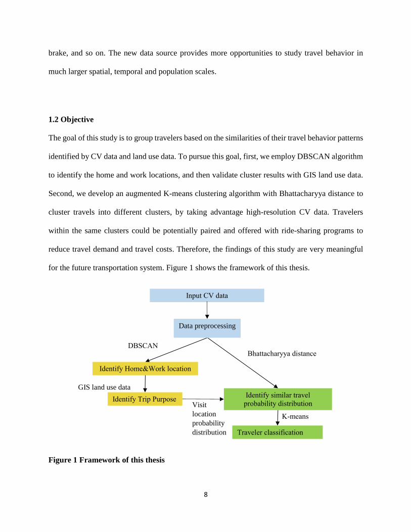
1.2 Objective
The goal of this study is to group travelers based on the similarities of their travel behavior patterns
identified by CV data and land use data. To pursue this goal, first, we employ DBSCAN algorithm
to identify the home and work locations, and then validate cluster results with GIS land use data.
Second, we develop an augmented K-means clustering algorithm with Bhattacharyya distance to
cluster travels into different clusters, by taking advantage high-resolution CV data. Travelers
within the same clusters could be potentially paired and offered with ride-sharing programs to
reduce travel demand and travel costs. Therefore, the findings of this study are very meaningful
for the future transportation system. Figure 1 shows the framework of this thesis.
Figure 1 Framework of this thesis
Input CV data
Identify Home&Work location
Identify Trip Purpose
DBSCAN
Identify similar travel
probability distribution
Traveler classification
Bhattacharyya distance
K-means
Data preprocessing
GIS land use data
Visit
location
probability
distribution

9
1.3 Thesis Organization
The rest of thesis is structured as follows: Chapter 2 conducts a comprehensive literature review.
Chapter 3 describes the methodology. Chapter 4 summarizes the basic statistics of the datasets
used for the case study. Chapter 5 demonstrates the numerical results. Moreover, Chapter 6
concludes with the major findings and the future research.
10
Chapter 2 Literature Review
2.1 Travel Behavior Data Analysis and Traveler Classification
Household trip data are crucial travel behavior data for travel demand forecasting and
transportation system planning. The survey-based methods used for trip data collection
experienced the stages of paper and pencil interviews (PAPI), computer-assisted telephone
interviews (CATI), and computer-assisted-self- interviews (CASI) (Wolf et al., 2001). Although
the computer-assisted interviews tried to help respondents to understand questions and recall trips
they had during a day, these methods are restricted by the accuracy of recall, reliability, and
compliance (Wu et al., 2011).
Recently, GPS and GIS technologies have been used to supplement the traditional survey data.
Wolf et al. (2001) used GPS data and GIS land use data to successfully identify 151 out of 156
trips provided by 13 participants. Bohte et al. (2008) also successfully identified travel
characteristics of individuals by using GPS and GIS data. Chen et al. (Chen et al., 2010) combined
GPS and GIS technologies to develop procedures and models for trip end clustering and trip
purpose prediction. However, the accuracy is influenced by dilution of precision of GPS logs and
inaccuracy in GIS database(Wolf et al., 2001). Kim et al. (2015) used Future Mobility Survey
(FMS) as an activity travel data collection method facilitated by a smartphone application or an
interactive web interface. It acquires time-space data by utilizing sensors such as GPS, Wifi and
Mobile Communication Systems (GSM, CDMA, and UMTS), and accelerometers. They used
ensemble-learning-based classification to recognize travel patterns from the FMS data collected in
Singapore. As found, more training days will help improve the overall model classification

11
accuracy for the seen users whose travel activity histories were used to train models. For the unseen
users, the classification performance improves as the training days accumulate more than those
used for seen users. Moreover, the classification accuracy for seen users is better than unseen
users, which indicates that learning from users’ own histories does help improve the classification
performance. Schonfelder et al. (2002) used a multi-stage hierarchical matching procedure to
calculate a cluster center of stop ends by combining trip ends, identifying trips with obvious
purposes with the socio-demographics of the respondents.
The method of deriving trip purposes based on GPS and GIS data was also incorporated into a
machine learning algorithm. Some researcher used decision tree based classifiers to derive trip
purposes. Lu et al. (2012) implemented a decision tree approach to identify trip purpose by using
GPS-based travel surveys. They found out that trip end locations can affect trip purpose
classification most and can improve more than 20% classification accuracy. Moreover, next and
previous trip information can improve more than 10% classification accuracy. However, social-
demographic of respondents only can improve less than 1% classification accuracy. Researchers
also implemented decision tree methods in C4.5, C5.0, or an adaptive boosting environment (Deng
and Ji, 2010, Griffin and Huang, 2005). Some of the research above require the social-economic
characteristics of respondents (such as age, gender and household income).
Researchers have also been making great efforts to classify travelers by using daily travel data and
socio-economic data. The criteria to select similarity measures depend on the analysts’ importance
ranking of various affecting attributes and the situations to be dealt with (Jones, 1990).
12
Consequently, of the resulting similarity measures could be subjective and case sensitive, and thus
derive quite inconsistent results. Hanson et al. (1986) divided individuals into five homogeneous
travel behavior groups by using complex multi-day travel data and explained variability in
individuals’ daily travels. Shoval et al. (2007) implemented a sequence alignment method based
on GPS data and clustered the data to three temporal-spatial time geographies. Kitamura and van
der Horn (1987) showed that daily participation could be very stable in different types of activities
(based on the categories of working, leisure, shopping and other activities). Axhausen et al. (2002)
collected six weeks continuous travel diaries from about 300,000 inhabitants in Germany in fall
1999. Hazard models were used to analyze this high-quality data. A low degree of spatial
variability of daily participation of activities was also found from the analysis.
The typical similarity indices rely on Euclidean distance or some measures used in signal
processing. Signal processing measures have been found vulnerable to process choice data. As for
the Euclidean-distance based measurement, instead of using traditional methods that purely rely
on conventional Euclidean distance, Joh et al. (2002) employed the alignment method to
distinguish different travel patterns. This breakthrough overcomes the problem that the traditional
Euclidean distance cannot deal with interdependent attributes. However, it still cannot capture
similarities and relations among sequential activities. As an improvement, we developed a
Bhattacharyya distance with K-means algorithm to measure similarities among sequential
activities.

13
Travel trajectory clustering becomes more and more prevalent recently. Kim et al. (2015) used
Longest Common Subsequence (LCS) to measure the similarity between two trajectories of
vehicles. Then they incorporate LCS with DBSCAN to distinct traffic flow clusters. Finally, they
employed Cluster Respresentive Subsequence (CRS) to allocate new trajectories into similar
clusters. Besse et al. (2016) used a different way to cluster vehicle trajectories. They developed a
new distance to compare trajectories which called Symmetrized Segment-Path Distance (SSPD).
2.2 Distribution-based Similarity Measures
Researchers mainly used tradition partitioning clustering methods such as k-means or KNN to
cluster uncertain data according to geometric distances between objects. Such methods cannot
handle uncertain objects that are geometrically distinguishable, such as datasets with the same
mean but with different variances.
Fortunately, measuring the similarity between different probability distributions of uncertain
objects can shed light on identifying similar uncertain objects. Researchers developed lots of
methods to assess the similarity between two distributions. Kullback-Leibler divergence is the
most prevalent one, which is a measure of the difference between two probability distributions P
and Q. By minimizing the Kullback-Leibler divergence, Bunte et al. (2010) dimensionally reduced
and visualized images from exploratory observation machine. However, Kullback-Leibler
divergence is never a real distance or metric. It does not follow the triangle inequality; it does not
have a boundary, and 𝐷𝐾𝐿(𝑃||𝑄)does not equal to 𝐷𝐾𝐿(𝑄||𝑃)in most scenarios. Moreover, it is
hard to compare, because𝐷𝐾𝐿(𝑃||𝑄) > 𝐷𝐾𝐿(𝑅||𝑄) does not mean that P is more similar to Q than
14
R. The infinitesimal form, specifically its Hessian, gives a metric tensor called Fisher information
metric. It is an information metric that can be used to similarities between uncertain objects. Frank
(2009) maximized the amount of Fisher information about environment captured by the population
and measured how natural selection influences evolutionary dynamics. Fisher information metric
also has a relationship with Jensen-Shanno divergence when being used to measure actions and
curve lengths. Jensen-Shanno is a prevailing method of determining the similarity between two
probability distributions. It is built on the Kullback-Leibler divergence.
However, it is symmetric and always returns a finite value. Grosse et al. (2002) analyzed symbolic
sequences using the Jensen-Shannon divergence, and applied this method to DNA sequences.
Nevertheless, Jensen-Shannon divergence requires probability distributions following a
multinomial distribution type. Wasserstein metric is a distance function defined between
probability distributions on a given metric space M. Ni et al. (2009) employed Wasserstein metric
to measure the distance between two histograms by comparing many pointwise distances. In
addition, it is robust to noisy data, and it is insensitive to oscillations. Similar as Kullback-Leibler
divergence, Hellinger distance is likewise a type of f-divergence. It is symmetric and has the
boundary as well as Jensen-Shanno. Sengar et al. (2008) developed a VoIP floods method using
the Hellinger distance successfully.
Bhattacharyya distance can also measure the similarity of two probability distributions that could
be discrete and continuous. It can be used to determine the relative closeness of two samples
according to the Bhattacharyya coefficient that measures the amount of overlapping between two
15
samples. The Bhattacharyya distance is widely used in research on feature extraction and selection
(Choi and Lee, 2003, Narendra and Fukunaga, 1977, Xuan et al., 2006), image processing (Goudail
et al., 2004), signal selection(Kailath, 1967), speaker recognition (You et al., 2009, Salvi, 2003)
and phone clustering (Mak and Barnard, 1996). In this thesis, we leverage the Bhattacharyya
distance to measure the distance between two distributions of travel attributes from two travelers.

16
Chapter 3 Methodology
3.1 DBSCAN
The Density-based spatial clustering of applications with noise (DBSCAN) is a kind of density-
based algorithm which can identify clusters of arbitrary shape in large longitudinal data sets by
looking at the local density of database elements. We can use this algorithm to identify home and
work locations in this thesis. This algorithm only uses one input parameter and can also determine
which points should be considered to be outliers or noise. There are two parameters defined in this
algorithm, Eps (maximum radius of the neighborhood) and MinPts (minimum number of points in
the Eps-neighborhood of a point). This algorithm consists of six definitions and two lemmas(Ester
et al., 1996). The most important definitions are density-reachable and density-connected which
are illustrated in Figure 2 and Figure 3 below. Moreover, DBSCAN algorithm process is also
showed below.
Algorithm 1 DBSCAN
Input: points
Figure 3 p and q are density-connected Figure 2 p and q are density-reachable

17
Output: clusters
1 for each 𝑝 ∈ 𝐷do
2 if p is not yet classified then
3 if p is a core point then
4 collect all objects density-reachable from p and assign them to a new cluster
5 else
6 assign p to noise
7 end
8 end
9 end
3.2 Bhattacharyya Distance
Bhattacharyya distance is a statistics method which measures the similarity of two discrete or
continuous probability distribution. It is closely related to the Bhattacharyya coefficient which can
measure the overlap area between two statistical samples or populations. This coefficient indicates
the relative similarity of two probability distribution. For two probability distribution p and q with
same parameter X, the Bhattacharyya distance is defined as follow:
𝐷𝐵(𝑝, 𝑞) = ln(𝐵𝐶(𝑝, 𝑞)) (1)
where 𝐵𝐶(𝑝, 𝑞) is the Bhattacharyya coefficient. Calculating the Bhattacharyya coefficient
involves a rudimentary form of integration of the overlap of the two samples. The interval of the
values of the two samples is split into a chosen number of partitions, and the number of members
of each sample in each partition is used in the following formula,
18
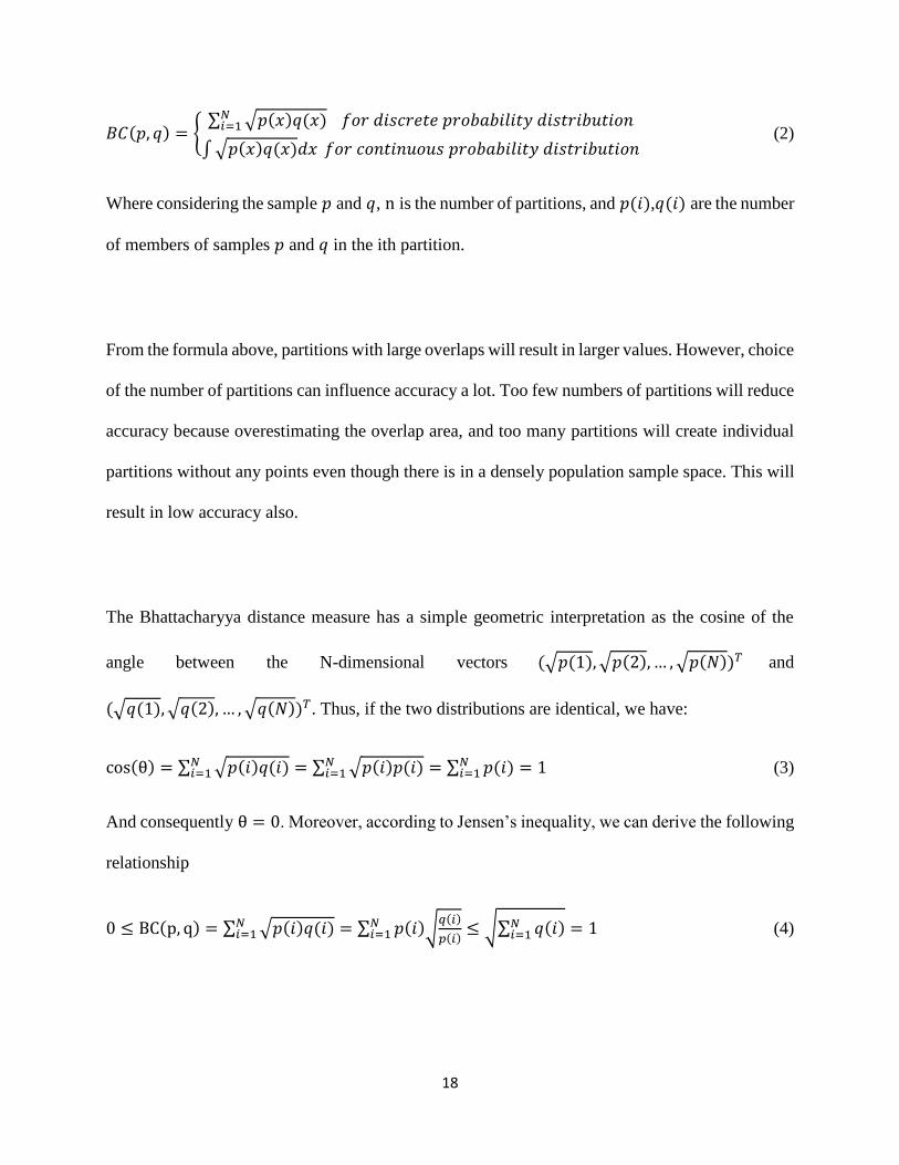
𝐵𝐶(𝑝, 𝑞) = {∑ √𝑝(𝑥)𝑞(𝑥)𝑁𝑖=1 𝑓𝑜𝑟𝑑𝑖𝑠𝑐𝑟𝑒𝑡𝑒𝑝𝑟𝑜𝑏𝑎𝑏𝑖𝑙𝑖𝑡𝑦𝑑𝑖𝑠𝑡𝑟𝑖𝑏𝑢𝑡𝑖𝑜𝑛
∫√𝑝(𝑥)𝑞(𝑥)𝑑𝑥 𝑓𝑜𝑟𝑐𝑜𝑛𝑡𝑖𝑛𝑢𝑜𝑢𝑠𝑝𝑟𝑜𝑏𝑎𝑏𝑖𝑙𝑖𝑡𝑦𝑑𝑖𝑠𝑡𝑟𝑖𝑏𝑢𝑡𝑖𝑜𝑛 (2)
Where considering the sample 𝑝 and 𝑞, n is the number of partitions, and 𝑝(𝑖),𝑞(𝑖) are the number
of members of samples 𝑝 and 𝑞 in the ith partition.
From the formula above, partitions with large overlaps will result in larger values. However, choice
of the number of partitions can influence accuracy a lot. Too few numbers of partitions will reduce
accuracy because overestimating the overlap area, and too many partitions will create individual
partitions without any points even though there is in a densely population sample space. This will
result in low accuracy also.
The Bhattacharyya distance measure has a simple geometric interpretation as the cosine of the
angle between the N-dimensional vectors (√𝑝(1),√𝑝(2),… ,√𝑝(𝑁))𝑇 and
(√𝑞(1),√𝑞(2), … ,√𝑞(𝑁))𝑇. Thus, if the two distributions are identical, we have:
cos(θ) = ∑ √𝑝(𝑖)𝑞(𝑖) = ∑ √𝑝(𝑖)𝑝(𝑖) = ∑ 𝑝(𝑖)𝑁𝑖=1 = 1𝑁
𝑖=1𝑁𝑖=1 (3)
And consequently θ = 0. Moreover, according to Jensen’s inequality, we can derive the following
relationship
0 ≤ BC(p, q) = ∑ √𝑝(𝑖)𝑞(𝑖) = ∑ 𝑝(𝑖)√𝑞(𝑖)
𝑝(𝑖)≤ √∑ 𝑞(𝑖)𝑁
𝑖=1 = 1𝑁𝑖=1
𝑁𝑖=1 (4)

19
Therefore, 0 ≤ BC(p, q) ≤ 1 and 0 ≤ 𝐷𝐵(𝑝, 𝑞) ≤ ∞. The Bhattacharyya coefficient will be 0 if
there is no overlap at all due to the multiplication by zero in every partition. This means the
distance between fully separated samples will not be exposed by this coefficient alone. The
Bhattacharyya coefficient will be 1 if these two probability distributions are exactly the same.
3.3 K-means
K-means is a prevalent unsupervised learning algorithm that resolves the clustering problem. The
key idea is define k centers, one for each cluster. Then minimize the squared error function for
points for all the cluster.
𝑎𝑟𝑔min𝑆∑ ∑ ||𝑥 − 𝜇𝑖||
2𝑥∈𝑆𝑖
𝑘𝑖=1 (5)
Where 𝜇𝑖 is the centroid or mean points in cluster 𝑆𝑖. Time-space data has huge amount of
information. If using points as centroids of clusters, we will lost information. Therefore, not like
traditional K-means algorithm, centroid of clusters are points. We developed an Augmented K-
means algorithm that centroid of clusters are probability distributions. In this thesis, instead
Euclidean distance for points, we employed Bhattacharyya coefficient in Bhattacharyya distance
to measure distance for probability distributions. Therefore, we rewrite the distance measurement
equation as follow,
argmin𝑆∑ ∑ ∑(1 − 𝐵𝐶(𝑥, 𝜇𝑖))𝑥∈𝑆𝑖𝑘𝑖=1 (6)
In order to minimize the object function, we write Bhattacharyya coefficient as √1 − 𝐵𝐶(𝑝, 1)
which is also called Hellinger distance.The centroids for each cluster will be recalculated after
cluster. In traditional K-means algorithm, a centroid is a point. In order to incorporate with

20
probability distribution, instead of points we use medial distributions. The medial distribution is
represented by mean of 15 quantiles, respectively. The process of augmented K-means algorithm
is show as follows.
Algorithm 2 Augmented K-means algorithm with Bhattacharyya distance
Input: ({𝑥1, 𝑥2, … , 𝑥𝑛}𝑐, K ),
Output: {𝜇1, 𝜇2, … , 𝜇𝑘}
1 (𝑆1, 𝑆2, … , 𝑆𝐾) ←Select random seeds ({𝑥1, 𝑥2, … , 𝑥𝑛}, K )
2 for k in 1: K
3 do 𝜇𝑘 ← 𝑆𝑘
4 while stopping criterion has not been met
5 do for k in 1:K
6 do 𝜔𝑘 ← {}
7 for n in 1:N
8 do j ← argmin𝑗′∑(1 − 𝐵𝐶(𝑥, 𝜇𝑖))
9 𝜔𝑗 ← 𝜔𝑗 ∪ {𝑥𝑛} (reassignment of vectors)
10 for k in 1:K
11 do 𝜇𝑘 ←1
|𝜔𝑘|∑ 𝑥𝑝𝑥∈𝜔𝑘 (recomputation of centroids, p is quantile)
12 end
13 end
14 end
15 end

21
Chapter 4 Data Description and Preliminary Analysis
In this thesis, raw trip data was acquired from a recently released CV dataset on Federal Highway
Administration (FHWA) research data exchange (RDE) website(FHWA, 2013). The dataset was
generated by safety pilot program, hosted by University of Michigan Transportation Research
Institution (UMTRI) in Ann Arbor, MI. Basic safety message (BSM) was extracted from CV
dataset. The BSM is a kind of ‘heartbeat’ message which transmits messages frequently (usually
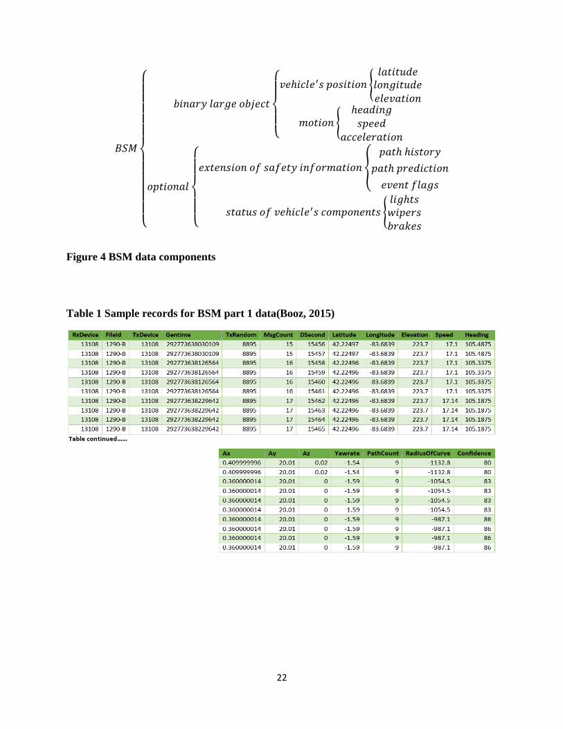
at approximately 10HZ, the same frequency of data used in this thesis). A BSM includes two parts;
one part is a binary large object (blob) that includes every BSM. It consists of fundamental data
elements that describe a vehicle’s position (latitude, longitude, and elevation) and motion (heading,
speed and acceleration). The other part of BSM data is optional one which contains an extension
of vehicle safety information (path history, path prediction and event flags) and pertains to the
status of a vehicle’s components (lights, wipers, and brakes). Figure 4 shows all the component of
BSM data. We only need the first part of BSM data in our research and data range is the whole
month of April 2013. Table 1 is the sample records of first part of BSM data, and Table 2 is the
sample records of a summary of first part of BSM data. The total size of these two datasets is 204
GB, and it consists of 216670 trips that made 2204 participants.
22
𝐵𝑆𝑀
{
𝑏𝑖𝑛𝑎𝑟𝑦 𝑙𝑎𝑟𝑔𝑒 𝑜𝑏𝑗𝑒𝑐𝑡
{
𝑣𝑒ℎ𝑖𝑐𝑙𝑒′𝑠 𝑝𝑜𝑠𝑖𝑡𝑖𝑜𝑛 {
𝑙𝑎𝑡𝑖𝑡𝑢𝑑𝑒𝑙𝑜𝑛𝑔𝑖𝑡𝑢𝑑𝑒𝑒𝑙𝑒𝑣𝑎𝑡𝑖𝑜𝑛
𝑚𝑜𝑡𝑖𝑜𝑛 {ℎ𝑒𝑎𝑑𝑖𝑛𝑔𝑠𝑝𝑒𝑒𝑑
𝑎𝑐𝑐𝑒𝑙𝑒𝑟𝑎𝑡𝑖𝑜𝑛
𝑜𝑝𝑡𝑖𝑜𝑛𝑎𝑙
{
𝑒𝑥𝑡𝑒𝑛𝑠𝑖𝑜𝑛 𝑜𝑓 𝑠𝑎𝑓𝑒𝑡𝑦 𝑖𝑛𝑓𝑜𝑟𝑚𝑎𝑡𝑖𝑜𝑛 {
𝑝𝑎𝑡ℎ ℎ𝑖𝑠𝑡𝑜𝑟𝑦
𝑝𝑎𝑡ℎ 𝑝𝑟𝑒𝑑𝑖𝑐𝑡𝑖𝑜𝑛
𝑒𝑣𝑒𝑛𝑡 𝑓𝑙𝑎𝑔𝑠
𝑠𝑡𝑎𝑡𝑢𝑠 𝑜𝑓 𝑣𝑒ℎ𝑖𝑐𝑙𝑒′𝑠 𝑐𝑜𝑚𝑝𝑜𝑛𝑒𝑛𝑡𝑠 {𝑙𝑖𝑔ℎ𝑡𝑠𝑤𝑖𝑝𝑒𝑟𝑠𝑏𝑟𝑎𝑘𝑒𝑠
Figure 4 BSM data components
Table 1 Sample records for BSM part 1 data(Booz, 2015)
23
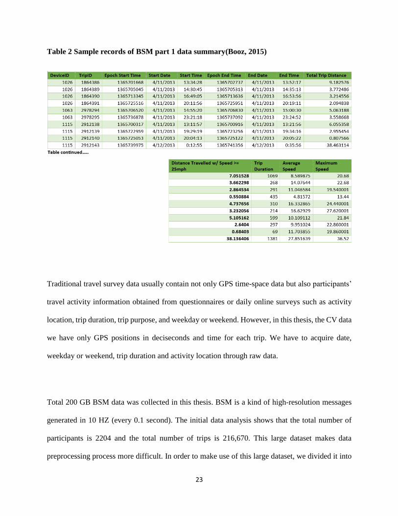
Table 2 Sample records of BSM part 1 data summary(Booz, 2015)
Traditional travel survey data usually contain not only GPS time-space data but also participants’
travel activity information obtained from questionnaires or daily online surveys such as activity
location, trip duration, trip purpose, and weekday or weekend. However, in this thesis, the CV data
we have only GPS positions in deciseconds and time for each trip. We have to acquire date,
weekday or weekend, trip duration and activity location through raw data.
Total 200 GB BSM data was collected in this thesis. BSM is a kind of high-resolution messages
generated in 10 HZ (every 0.1 second). The initial data analysis shows that the total number of
participants is 2204 and the total number of trips is 216,670. This large dataset makes data
preprocessing process more difficult. In order to make use of this large dataset, we divided it into
24
100 partitions. Further, according to the summary of BSM part 1 data, we find out trip information
for each trip of each DeviceID (participant). As the base of each trip, we extracted position
information from BSM part 1 dataset with the same DeviceID and within traveling time window
(Gentime of BSM part 1 data is between Start Time and End Time of each trip) and assigned the
same TripID as the base trip. Since the rule to get Gentime in Table 1 is not same as Epoch
Start/End Time in Table 2. Gentime is the number of milliseconds has elapsed since midnight,
January 1, 2004 in UTC time with 35 seconds offset (Booz, 2015). Whereas, Epoch Start/End
Time is Unix time which is the number of seconds has elapsed since midnight, January 1, 1970.
So we used different rules to translate timestamp variables into the same scale. After this stage, we
merged BSM part 1 data and summary of BSM part 1 data together and obtained every 0.1 second
position for each trip of each participant. Also, trip start and end locations can detect from the big
new merged table. We considered the first position of one trip is the trip start location and the last
position is the trip end location after sorted trip data by Gentime.
Then we could use machine learning methods to mine trip purpose according to trip end for each
trip. It is generally believed that it is not necessary for everyone having a job, but everyone should
have a home location. Therefore, this thesis assumes that the location that individuals most
frequently reported is home, followed by working place. Hence, we used Density-based spatial
clustering of applications with noise (DBSCAN) which is the most prevalent density-base
clustering method to identify home and work location. The location with the highest density of trip
end was configured as home followed by workplaces. After identifying the home and work
location for each participant, we used land use data in geographic information system (GIS) to
verify the accuracy for home position clustering (There should be at least one land use parcel with
25
residential land-use within 500m area of the clustered home position). We loosen the home
location area to 500m region in order to avoid dilution of precision of GPS system and driveway
parking.
After using DBSCAN algorithm, we found both home and work locations for 667 participants and
only home locations for 397 participants. We cannot identify home and work locations for 166
individuals.
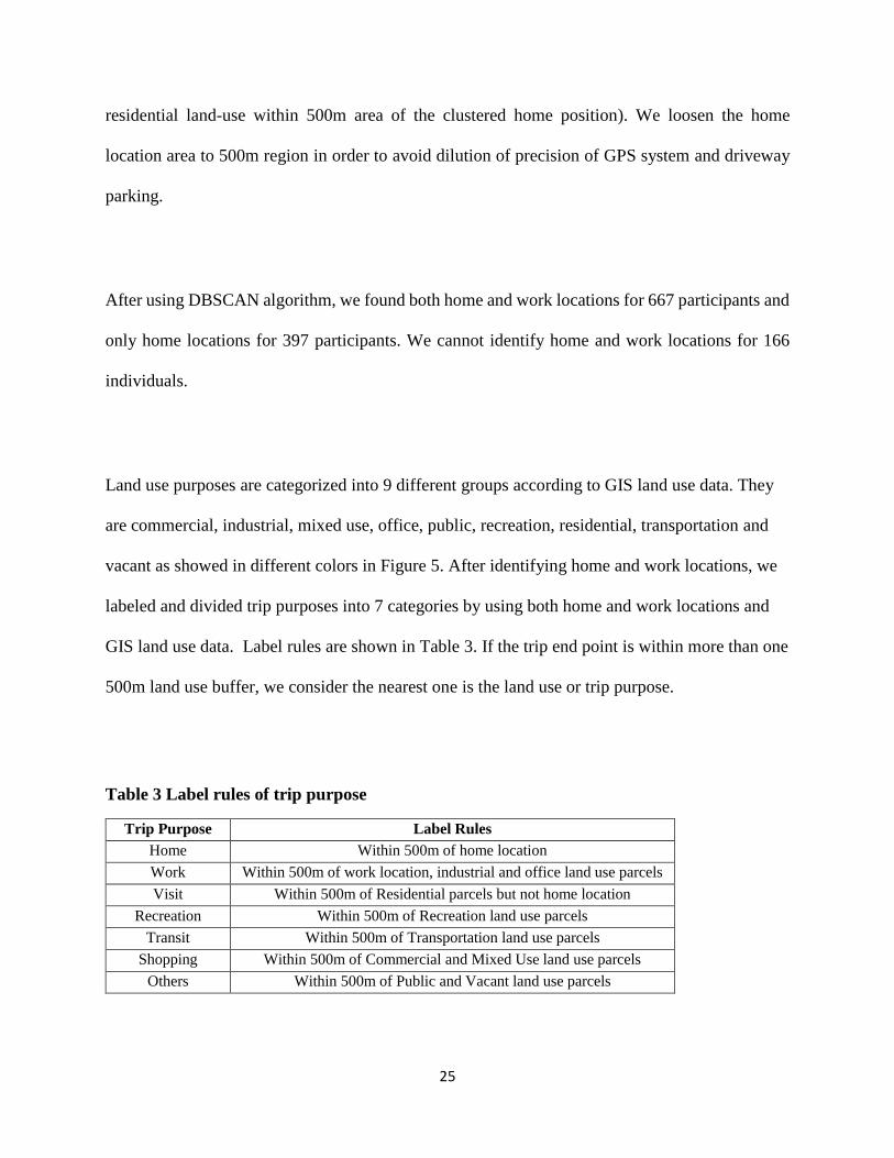
Land use purposes are categorized into 9 different groups according to GIS land use data. They
are commercial, industrial, mixed use, office, public, recreation, residential, transportation and
vacant as showed in different colors in Figure 5. After identifying home and work locations, we
labeled and divided trip purposes into 7 categories by using both home and work locations and
GIS land use data. Label rules are shown in Table 3. If the trip end point is within more than one
500m land use buffer, we consider the nearest one is the land use or trip purpose.
Table 3 Label rules of trip purpose
Trip Purpose Label Rules
Home Within 500m of home location
Work Within 500m of work location, industrial and office land use parcels
Visit Within 500m of Residential parcels but not home location
Recreation Within 500m of Recreation land use parcels
Transit Within 500m of Transportation land use parcels
Shopping Within 500m of Commercial and Mixed Use land use parcels
Others Within 500m of Public and Vacant land use parcels
26
Individual travel trajectories can be utilized to uncover human behavioral characteristic. Figure 5
illustrates all trip ends for all participants during one month. Figure 6 shows daily trajectories
reported by a vehicle during a week. As can be seen from the daily trajectory plots, a similar route
between home and the workplace was repeatedly used during weekdays while very different
trajectories were reported during weekends. Figure 7 shows the hourly trajectories. The departure
time is still consistent and return time is almost the same. In this figure, purple lines mean trip
purposes are industry, and yellow lines mean home based trips. The green lines at the bottom of
both figures are the projection of all trajectories. Levy Flight pattern is a pattern characterized by
many short-distance trips connected by long-distance relocations. Short-distance trips are mainly
composed of commuting to work or supermarket shopping. On the contrary, long-distance trips
mostly comprise rare and infrequent events. There are three widely accepted and used indicators:
the trip distance distribution 𝑝(𝑟), the radius of gyration (ROG) 𝑟𝑔(𝑡) and the number of visited
locations 𝑆(𝑡) over time. We use these three indicators to identify different travel behavior. During
the working day, some people just have to commute trip between home and work place. However,
some people have social activities after work. On the weekend, someone likes to stay at home.
Whereas, someone prefers to go out and enjoy their weekend in the city or even have long-distance
intercity trips.

27
Figure 5 The map of land use data with all trip ends in Ann Arbor, MI

28
Figure 6 Daily CV trajectories during a week
Figure 7 Multiple one-day CV trajectories
29
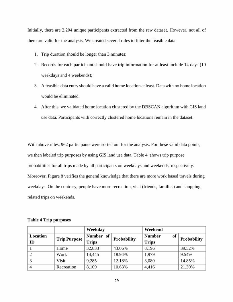
Initially, there are 2,204 unique participants extracted from the raw dataset. However, not all of
them are valid for the analysis. We created several rules to filter the feasible data.
1. Trip duration should be longer than 3 minutes;
2. Records for each participant should have trip information for at least include 14 days (10
weekdays and 4 weekends);
3. A feasible data entry should have a valid home location at least. Data with no home location
would be eliminated.
4. After this, we validated home location clustered by the DBSCAN algorithm with GIS land
use data. Participants with correctly clustered home locations remain in the dataset.
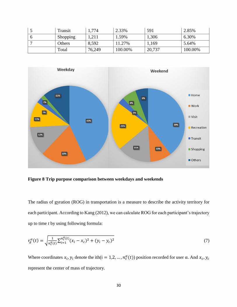
With above rules, 962 participants were sorted out for the analysis. For these valid data points,
we then labeled trip purposes by using GIS land use data. Table 4 shows trip purpose
probabilities for all trips made by all participants on weekdays and weekends, respectively.
Moreover, Figure 8 verifies the general knowledge that there are more work based travels during
weekdays. On the contrary, people have more recreation, visit (friends, families) and shopping
related trips on weekends.
Table 4 Trip purposes
Weekday Weekend
Location
ID Trip Purpose
Number of
Trips Probability
Number of
Trips Probability
1 Home 32,833 43.06% 8,196 39.52%
2 Work 14,445 18.94% 1,979 9.54%
3 Visit 9,285 12.18% 3,080 14.85%
4 Recreation 8,109 10.63% 4,416 21.30%
30
5 Transit 1,774 2.33% 591 2.85%
6 Shopping 1,211 1.59% 1,306 6.30%
7 Others 8,592 11.27% 1,169 5.64%
Total 76,249 100.00% 20,737 100.00%
Figure 8 Trip purpose comparison between weekdays and weekends
The radius of gyration (ROG) in transportation is a measure to describe the activity territory for
each participant. According to Kang (2012), we can calculate ROG for each participant’s trajectory
up to time t by using following formula:
𝑟𝑔𝛼(𝑡) = √
1
𝑛𝑐𝛼(𝑡)
∑ (𝑥𝑖 − 𝑥𝑐)2 + (𝑦𝑖 − 𝑦𝑐)2𝑛𝑐𝛼(𝑡)
𝑖=1 (7)
Where coordinates 𝑥𝑖 , 𝑦𝑖 denote the ith(i = 1,2, … , 𝑛𝑐𝛼(𝑡)) position recorded for user α. And 𝑥𝑐 , 𝑦𝑐
represent the center of mass of trajectory.

31
Figure 9 ROG probability distributions
In Figure 9, the blue dashed line is the ROG calculated when the geometric center of all trip ends
is considered the center of a trajectory, and the red line is the ROG when the location of home is
treated as the center of trajectory. We found that these two ROG distributions are almost the same.
Because ROG mostly depends on the frequent location, and home-based trips are the most frequent
trips in the daily travel, blue dashed line and red line are almost overlapped with each other. The
peak value for this ROG distribution is approximately 8 kilometers. The right skewness of ROG
distribution with trip reached around 40 kilometers, or less indicates that a large portion of
participants have their trips concentrated within a small activity territory, whereas only rare
individuals travel a longer distance in a daily base. We also found more information from this
figure that there is a significant effect of distance decay. Moreover, based on probability
distribution above, more than 95% of the participants have ROG values less than 40 kilometers,
and most of them are around 8 kilometers.
32
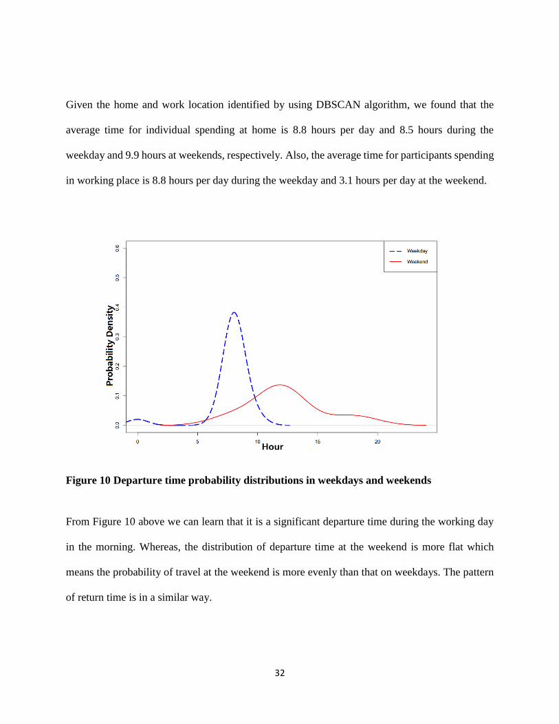
Given the home and work location identified by using DBSCAN algorithm, we found that the
average time for individual spending at home is 8.8 hours per day and 8.5 hours during the
weekday and 9.9 hours at weekends, respectively. Also, the average time for participants spending
in working place is 8.8 hours per day during the weekday and 3.1 hours per day at the weekend.
Figure 10 Departure time probability distributions in weekdays and weekends
From Figure 10 above we can learn that it is a significant departure time during the working day
in the morning. Whereas, the distribution of departure time at the weekend is more flat which
means the probability of travel at the weekend is more evenly than that on weekdays. The pattern
of return time is in a similar way.
33
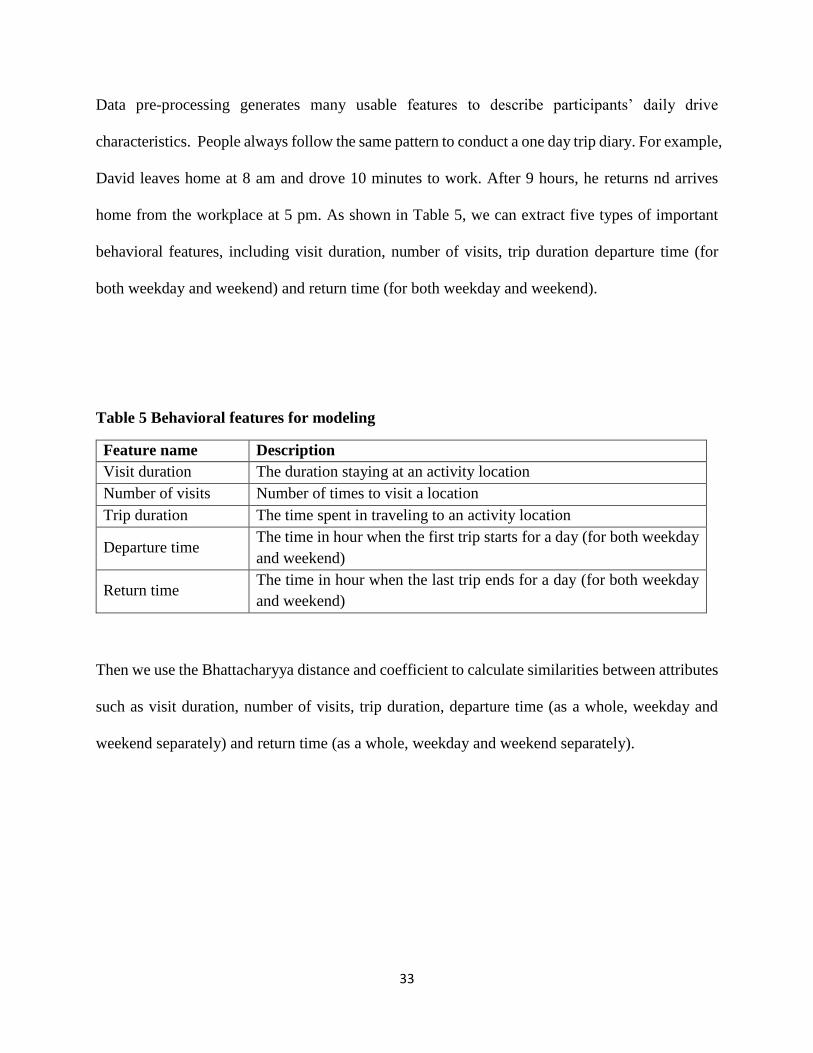
Data pre-processing generates many usable features to describe participants’ daily drive
characteristics. People always follow the same pattern to conduct a one day trip diary. For example,
David leaves home at 8 am and drove 10 minutes to work. After 9 hours, he returns nd arrives
home from the workplace at 5 pm. As shown in Table 5, we can extract five types of important
behavioral features, including visit duration, number of visits, trip duration departure time (for
both weekday and weekend) and return time (for both weekday and weekend).
Table 5 Behavioral features for modeling
Feature name Description
Visit duration The duration staying at an activity location
Number of visits Number of times to visit a location
Trip duration The time spent in traveling to an activity location
Departure time The time in hour when the first trip starts for a day (for both weekday
and weekend)
Return time The time in hour when the last trip ends for a day (for both weekday
and weekend)
Then we use the Bhattacharyya distance and coefficient to calculate similarities between attributes
such as visit duration, number of visits, trip duration, departure time (as a whole, weekday and
weekend separately) and return time (as a whole, weekday and weekend separately).

34
Figure 11 Visiting duration (for all data) probability distributions of two travelers with
high similarity (Bhattacharyya distance=0.99)
Figure 12 Trip duration (for all data) probability distributions of two travelers with high
similarity (Bhattacharyya distance=0.99)

35
Figure 13 Departure time (only on weekdays) probability distributions of two travelers
with high similarity (Bhattacharyya distance=0.99)
Figure 14 Return time (only on weekdays) probability distributions of two travelers with
high similarity (Bhattacharyya distance=0.99)
36
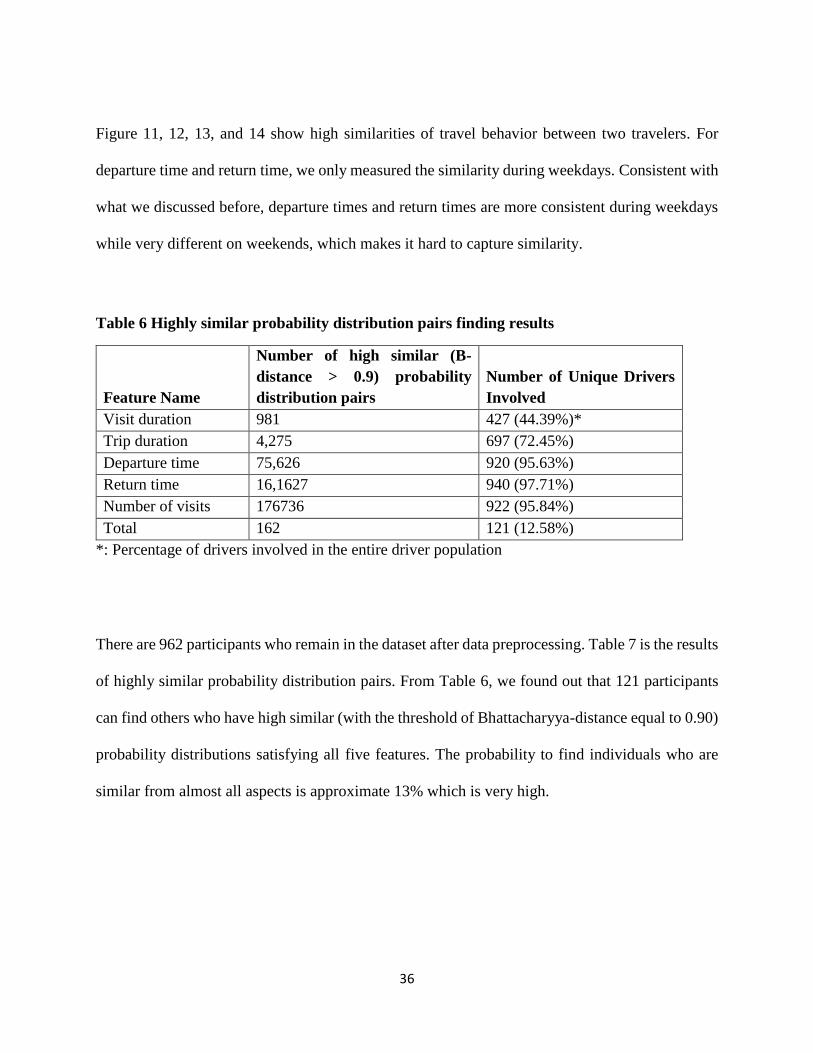
Figure 11, 12, 13, and 14 show high similarities of travel behavior between two travelers. For
departure time and return time, we only measured the similarity during weekdays. Consistent with
what we discussed before, departure times and return times are more consistent during weekdays
while very different on weekends, which makes it hard to capture similarity.
Table 6 Highly similar probability distribution pairs finding results
Feature Name
Number of high similar (B-
distance > 0.9) probability
distribution pairs
Number of Unique Drivers
Involved
Visit duration 981 427 (44.39%)*
Trip duration 4,275 697 (72.45%)
Departure time 75,626 920 (95.63%)
Return time 16,1627 940 (97.71%)
Number of visits 176736 922 (95.84%)
Total 162 121 (12.58%)
*: Percentage of drivers involved in the entire driver population
There are 962 participants who remain in the dataset after data preprocessing. Table 7 is the results
of highly similar probability distribution pairs. From Table 6, we found out that 121 participants
can find others who have high similar (with the threshold of Bhattacharyya-distance equal to 0.90)
probability distributions satisfying all five features. The probability to find individuals who are
similar from almost all aspects is approximate 13% which is very high.

37
Chapter 5 Clustering Results
In order to cluster individuals with high similarities, we develop an augmented K-means algorithm
to cluster travelers according to visit duration, number of visits, trip duration, departure time, and
return time. We try a different number of clusters and found out that 3 is the best number of clusters.
This makes all features are most homogenous within each cluster and heterogenic among all the
clusters.
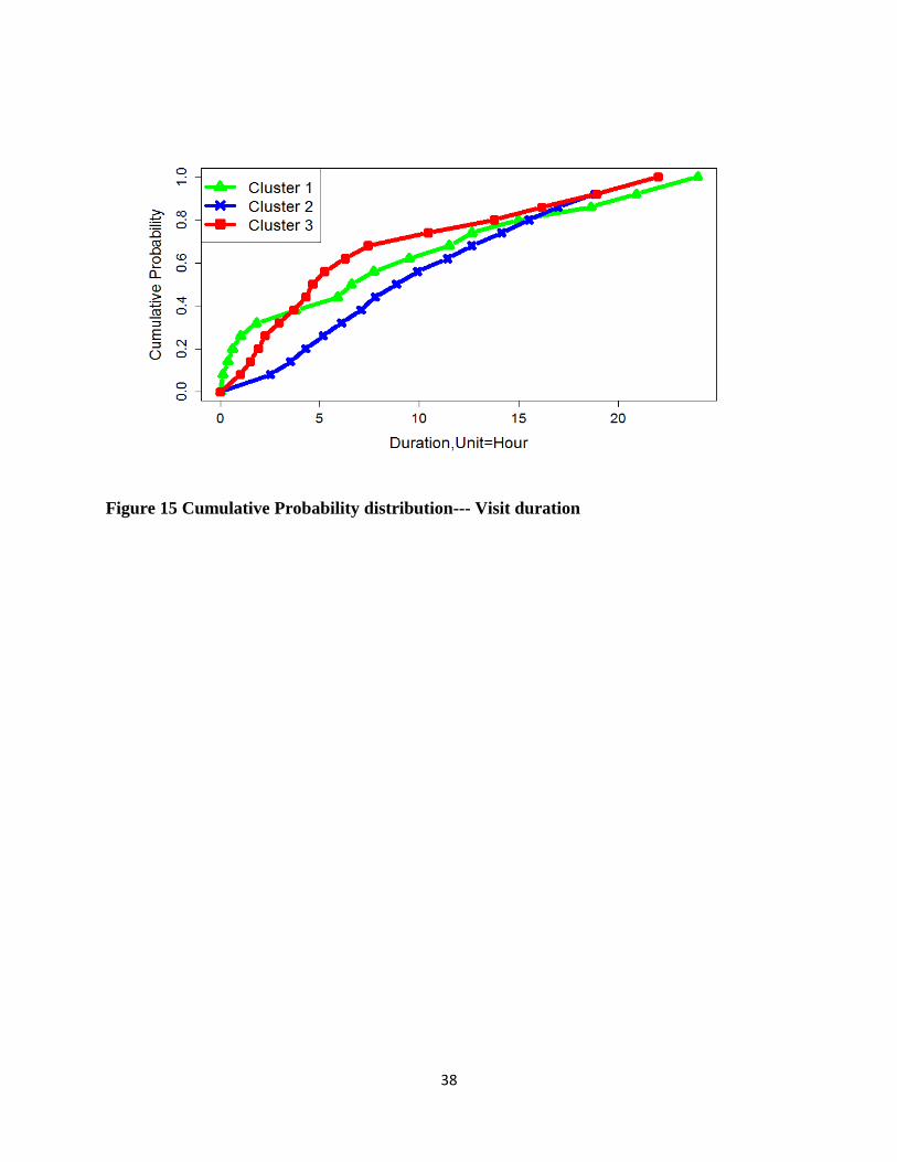
Figure 15 shows a cumulative probability distribution for visit duration. In this figure, cluster 2
has a longer visit duration than other two clusters. Figure 16 is a cumulative probability distribution
for number of visits. This figure contains lots of information. First, cluster 1 has more visit location
types than other two clusters, which mean people in cluster 1 may have more activities other than
home and work. Moreover, from lines of cluster 2 and cluster 3 we find out that home and work
based trips can cover approximate 70% of total trips. This result verifies that the finding in Section
2 that most individuals have low degrees of spatial variability. From Figure 17, we can get that
cluster 2 has the longest trip duration, and then follows cluster 3. Cluster 1 has the shortest trip
duration. Figure 18 presents a cumulative probability distribution for departure time. We can see
that cluster 1 always depart late and most departure time even at afternoon. Cluster 2 and cluster
3 almost depart at the same time, but people cluster 2 depart little earlier than individuals cluster
3. Figure 19 depicts the cumulative probability distribution for return time. Return time for cluster
2 and cluster 3 is similar. However, return time for individuals in cluster 1 is later than other 2
clusters.
38
Figure 15 Cumulative Probability distribution--- Visit duration

39
Figure 16 Cumulative probability distribution---Number of visits
Figure 17 Cumulative probability distribution---Trip duration

40
Figure 18 Cumulative probability distribution---Departure time
Figure 19 Cumulative probability distribution---Return time
41
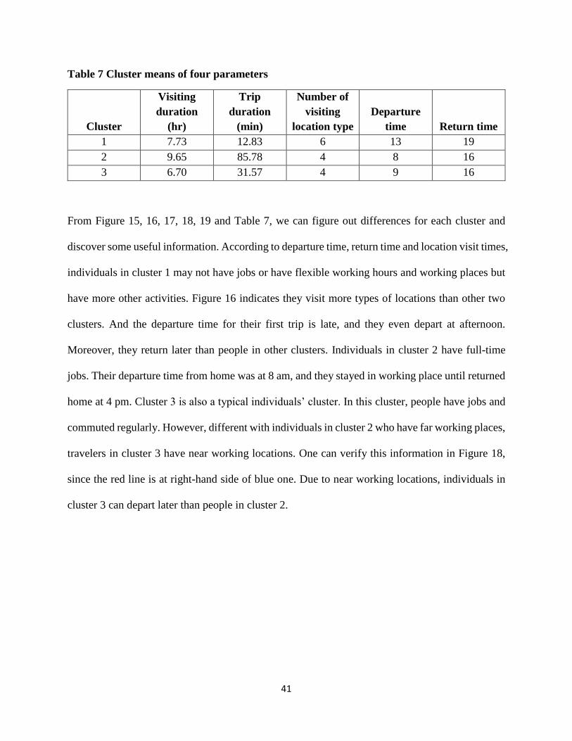
Table 7 Cluster means of four parameters
Cluster
Visiting
duration
(hr)
Trip
duration
(min)
Number of
visiting
location type
Departure
time Return time
1 7.73 12.83 6 13 19
2 9.65 85.78 4 8 16
3 6.70 31.57 4 9 16
From Figure 15, 16, 17, 18, 19 and Table 7, we can figure out differences for each cluster and
discover some useful information. According to departure time, return time and location visit times,
individuals in cluster 1 may not have jobs or have flexible working hours and working places but
have more other activities. Figure 16 indicates they visit more types of locations than other two
clusters. And the departure time for their first trip is late, and they even depart at afternoon.
Moreover, they return later than people in other clusters. Individuals in cluster 2 have full-time
jobs. Their departure time from home was at 8 am, and they stayed in working place until returned
home at 4 pm. Cluster 3 is also a typical individuals’ cluster. In this cluster, people have jobs and
commuted regularly. However, different with individuals in cluster 2 who have far working places,
travelers in cluster 3 have near working locations. One can verify this information in Figure 18,
since the red line is at right-hand side of blue one. Due to near working locations, individuals in
cluster 3 can depart later than people in cluster 2.
42
Chapter 6 Conclusions and Future Research
6.1 Conclusions
In this thesis, we use the time-space trajectory data collected by Connected Vehicles (CV) and
land use data to analyze travel behavior. We find some interesting observations after processing
the raw data and using the DBSCAN clustering method to identify home and work locations. First,
the results confirm some common sense of travel behavior. Individual travelers make more
commute trips to work during weekdays but more recreation, shopping and visiting trips on
weekends. Second, most participants’ travel territory is around eight kilometers, and 95%
participants travel within 40 kilometers for each trip. Third, most individuals have a low degree of
spatial variability, indicating that home and work based trips can cover about 70% of total trips.
Fourth, we employ Bhattacharyya distance and coefficient to find similar travel trajectories by
using travel attributes such as visit duration, number of visits, trip duration, departure time and
return time. Based on the analysis, we identify travelers who have similar travel patterns and thus
may be paired in ride-sharing applications. Finally, we develop an augmented k-mean algorithm
to classify drivers into three clusters, such as represent commute workers with near working places,
workers with far working places and individuals who do not have jobs or have flexible working
hours and working places but travel for other activates, respectively.
6.2 Future Research
In future, travel information and social-demographics data will be taken into account to enhance
the result and improve accuracy. Moreover, some existing drawbacks of time-space data, for
example, buildings or heavy foliage can block satellite signals, losing signal when going through
43
tunnels and dilution of precision of GPS data may be overcome in near future with the development
of GPS and the Connected Vehicles technology. Therefore, we can acquire more passive, accurate
time-space data. Furthermore, the analysis of similar driver behavior can go one step further. We
can cluster similar drivers by their daily travel trajectories that are a crucial part in ride-sharing
research. Moreover, we also can incorporate this information in the activity-based model to
conduct accurate travel demand forecasting.
44
References
AXHAUSEN, K. W., ZIMMERMANN, A., SCHÖNFELDER, S., RINDSFÜSER, G. & HAUPT, T. 2002. Observing
the rhythms of daily life: A six-week travel diary. Transportation, 29, 95-124.
BESSE, P. C., GUILLOUET, B., LOUBES, J.-M. & ROYER, F. 2016. Review and Perspective for Distance-Based
Clustering of Vehicle Trajectories.
BOHTE, W. & MAAT, K. Deriving and Validating Trip Destinations and Modes for Multiday GPS-Based
Travel Surveys: Application in the Netherlands. Transportation research board 87th annual
meeting, 2008.
BOOZ, A., HAMILTON 2015. Safety Pilot Model Devployment-Sample Data Environment Data Handbook.
US Department of Tansportation.
BUNTE, K., HAMMER, B., VILLMANN, T., BIEHL, M. & WISMÜLLER, A. Exploratory Observation Machine
(XOM) with Kullback-Leibler Divergence for Dimensionality Reduction and Visualization. ESANN,
2010. 87-92.
CHEN, C., GONG, H., LAWSON, C. & BIALOSTOZKY, E. 2010. Evaluating the feasibility of a passive travel
survey collection in a complex urban environment: Lessons learned from the New York City case
study. Transportation Research Part A: Policy and Practice, 44, 830-840.
CHEN, C., MA, J., SUSILO, Y., LIU, Y. & WANG, M. 2016. The promises of big data and small data for travel
behavior (aka human mobility) analysis. Transportation Research Part C: Emerging Technologies,
68, 285-299.
CHOI, E. & LEE, C. 2003. Feature extraction based on the Bhattacharyya distance. Pattern Recognition,
36, 1703-1709.
CICI, B., MARKOPOULOU, A., FRIAS-MARTINEZ, E. & LAOUTARIS, N. Assessing the potential of ride-
sharing using mobile and social data: a tale of four cities. Proceedings of the 2014 ACM
International Joint Conference on Pervasive and Ubiquitous Computing, 2014. ACM, 201-211.

45
DENG, Z. & JI, M. 2010. Deriving rules for trip purpose identification from GPS travel survey data and
land use data: A machine learning approach. Traffic and Transportation Studies, 2010, 768-777.
ESTER, M., KRIEGEL, H.-P., SANDER, J. & XU, X. A density-based algorithm for discovering clusters in large
spatial databases with noise. Kdd, 1996. 226-231.
FHWA, F. H. A. 2013. Connected Vehicle Research.
FRANK, S. A. 2009. Natural selection maximizes Fisher information. Journal of Evolutionary Biology, 22,
231-244.
GONG, L., MORIKAWA, T., YAMAMOTO, T. & SATO, H. 2014. Deriving personal trip data from GPS data: a
literature review on the existing methodologies. Procedia-Social and Behavioral Sciences, 138,
557-565.
GONZALEZ, M. C., HIDALGO, C. A. & BARABASI, A.-L. 2008. Understanding individual human mobility
patterns. Nature, 453, 779-782.
GOUDAIL, F., RÉFRÉGIER, P. & DELYON, G. 2004. Bhattacharyya distance as a contrast parameter for
statistical processing of noisy optical images. JOSA A, 21, 1231-1240.
GRIFFIN, T. & HUANG, Y. A decision tree classification model to automate trip purpose derivation. The
Proceedings of the ISCA 18th International Conference on Computer Applications in Industry
and Engineering, 2005. Citeseer, 44-49.
GROSSE, I., BERNAOLA-GALVÁN, P., CARPENA, P., ROMÁN-ROLDÁN, R., OLIVER, J. & STANLEY, H. E. 2002.
Analysis of symbolic sequences using the Jensen-Shannon divergence. Physical Review E, 65,
041905.
HANSON, S. & HUFF, J. 1986. Classification issues in the analysis of complex travel behavior.
Transportation, 13, 271-293.
46
JOH, C.-H., ARENTZE, T., HOFMAN, F. & TIMMERMANS, H. 2002. Activity pattern similarity: a
multidimensional sequence alignment method. Transportation Research Part B: Methodological,
36, 385-403.
JONES, P. 1990. Developments in dynamic and activity-based approaches to travel analysis, Avebury.
KAILATH, T. 1967. The divergence and Bhattacharyya distance measures in signal selection. IEEE
transactions on communication technology, 15, 52-60.
KANG, C., MA, X., TONG, D. & LIU, Y. 2012. Intra-urban human mobility patterns: An urban morphology
perspective. Physica A: Statistical Mechanics and its Applications, 391, 1702-1717.
KIM, J. & MAHMASSANI, H. S. 2015. Spatial and temporal characterization of travel patterns in a traffic
network using vehicle trajectories. Transportation Research Part C: Emerging Technologies, 59,
375-390.
KIM, Y., PEREIRA, F. C., ZHAO, F., GHORPADE, A., ZEGRAS, P. C. & BEN-AKIVA, M. 2015. Activity
recognition for a smartphone and web based travel survey. arXiv preprint arXiv:1502.03634.
KITAMURA, R. & VAN DER HOORN, T. 1987. Regularity and irreversibility of weekly travel behavior.
Transportation, 14, 227-251.
LU, Y., ZHU, S. & ZHANG, L. A Machine Learning Approach to Trip Purpose Imputation in GPS-Based
Travel Surveys. 4th Conference on Innovations in Travel Modeling, Tampa, Fla, 2012.
MAK, B. & BARNARD, E. Phone clustering using the Bhattacharyya distance. Spoken Language, 1996.
ICSLP 96. Proceedings., Fourth International Conference on, 1996. IEEE, 2005-2008.
NARENDRA, P. M. & FUKUNAGA, K. 1977. A branch and bound algorithm for feature subset selection.
IEEE Transactions on Computers, 100, 917-922.
NI, K., BRESSON, X., CHAN, T. & ESEDOGLU, S. 2009. Local histogram based segmentation using the
Wasserstein distance. International journal of computer vision, 84, 97-111.

47
SALVI, G. Accent clustering in Swedish using the Bhattacharyya distance. 15th International Congress of
Phonetic Science, 2003. 1149-1152.
SCHÖNFELDER, S. & ANTILLE, N. 2002. Exploring the potentials of automatically collected GPS data for
travel behaviour analysis: A Swedish data source, ETH, Eidgenössische Technische Hochschule
Zürich, Institut für Verkehrsplanung, Transporttechnik, Strassen-und Eisenbahnbau IVT.
SENGAR, H., WANG, H., WIJESEKERA, D. & JAJODIA, S. 2008. Detecting VoIP floods using the Hellinger
distance. IEEE transactions on parallel and distributed systems, 19, 794-805.
SHOVAL, N. & ISAACSON, M. 2007. Sequence alignment as a method for human activity analysis in space
and time. Annals of the Association of American geographers, 97, 282-297.
USDOT, U. S. D. O. T. 2016. Connected Vehicle Pilot Deployment Program.
WOLF, J., GUENSLER, R. & BACHMAN, W. 2001. Elimination of the travel diary: Experiment to derive trip
purpose from global positioning system travel data. Transportation Research Record: Journal of
the Transportation Research Board, 125-134.
WU, J., JIANG, C., HOUSTON, D., BAKER, D. & DELFINO, R. 2011. Automated time activity classification
based on global positioning system (GPS) tracking data. Environmental Health, 10, 1.
XUAN, G., ZHU, X., CHAI, P., ZHANG, Z., SHI, Y. Q. & FU, D. Feature selection based on the Bhattacharyya
distance. 18th International Conference on Pattern Recognition (ICPR'06), 2006. IEEE, 1232-
1235.
YOU, C. H., LEE, K. A. & LI, H. A GMM supervector Kernel with the Bhattacharyya distance for SVM based
speaker recognition. 2009 IEEE International Conference on Acoustics, Speech and Signal
Processing, 2009. IEEE, 4221-4224.