behavior characterization and development of lrfd

Graduate Theses and Dissertations Iowa State University Capstones, Theses andDissertations

2010

Behavior characterization and development ofLRFD resistance factors for axially-loaded steelpiles in bridge foundationsSherif Sayed AbdelsalamIowa State University

Follow this and additional works at: https://lib.dr.iastate.edu/etd

Part of the Civil and Environmental Engineering Commons

This Dissertation is brought to you for free and open access by the Iowa State University Capstones, Theses and Dissertations at Iowa State UniversityDigital Repository. It has been accepted for inclusion in Graduate Theses and Dissertations by an authorized administrator of Iowa State UniversityDigital Repository. For more information, please contact [email protected].

Recommended CitationAbdelsalam, Sherif Sayed, "Behavior characterization and development of LRFD resistance factors for axially-loaded steel piles inbridge foundations" (2010). Graduate Theses and Dissertations. 11347.https://lib.dr.iastate.edu/etd/11347

http://lib.dr.iastate.edu/?utm_source=lib.dr.iastate.edu%2Fetd%2F11347&utm_medium=PDF&utm_campaign=PDFCoverPages

http://lib.dr.iastate.edu/?utm_source=lib.dr.iastate.edu%2Fetd%2F11347&utm_medium=PDF&utm_campaign=PDFCoverPages

https://lib.dr.iastate.edu/etd?utm_source=lib.dr.iastate.edu%2Fetd%2F11347&utm_medium=PDF&utm_campaign=PDFCoverPages

https://lib.dr.iastate.edu/theses?utm_source=lib.dr.iastate.edu%2Fetd%2F11347&utm_medium=PDF&utm_campaign=PDFCoverPages

https://lib.dr.iastate.edu/theses?utm_source=lib.dr.iastate.edu%2Fetd%2F11347&utm_medium=PDF&utm_campaign=PDFCoverPages

https://lib.dr.iastate.edu/etd?utm_source=lib.dr.iastate.edu%2Fetd%2F11347&utm_medium=PDF&utm_campaign=PDFCoverPages

http://network.bepress.com/hgg/discipline/251?utm_source=lib.dr.iastate.edu%2Fetd%2F11347&utm_medium=PDF&utm_campaign=PDFCoverPages

https://lib.dr.iastate.edu/etd/11347?utm_source=lib.dr.iastate.edu%2Fetd%2F11347&utm_medium=PDF&utm_campaign=PDFCoverPages

mailto:[email protected]

Behavior characterization and development of LRFD resistance factors for axially-

loaded steel piles in bridge foundations

by

Sherif S. AbdelSalam

A dissertation submitted to the graduate faculty

in partial fulfillment of the requirements for the degree of

DOCTOR OF PHILOSOPHY

Major: Civil Engineering (Geotechnical Engineering)

Program of Study Committee:

Sri Sritharan, Major Professor

Muhannad T. Suleiman

Fouad S. Fanous

Thomas J. Rudolphi

Jeramy C. Ashlock

Charles T. Jahren

Iowa State University

Ames, Iowa

2010

ii

DEDICATION

The author devotes this thesis to his father Dr. Sayed AbdelSalam for his support and

inspiration throughout this work, as well as his mother, sister, and brother for their

unconditional support and understanding that helped the author to get through all the

challenges and successfully complete this thesis.

iii

TABLE OF CONTENTS

LIST OF FIGURES ..................................................................................................................... viii

LIST OF TABLES ....................................................................................................................... xiii

ABSTRACT ...................................................................................................................................xv

CHAPTER 1: INTRODUCTION ....................................................................................................1

1.1. Background ..............................................................................................................1

1.1.1. LRFD implementation.................................................................................3

1.1.2. Pile settlement .............................................................................................4

1.2. Scope of Research ....................................................................................................8

1.3. Thesis Outline ........................................................................................................10

1.4. References ..............................................................................................................12

CHAPTER 2: LITERATURE REVIEW .......................................................................................15

2.1. Allowable Stress Design ........................................................................................15

2.2. Load and Resistance Factor Design .......................................................................16

2.2.1. Basic principles .........................................................................................16

2.2.2. Implementation..........................................................................................17

2.2.3. Calibration by fitting to ASD ....................................................................18

2.2.4. Calibration using reliability theory ...........................................................20

2.2.5. Target reliability index ..............................................................................25

2.3. Framework for Calibration ....................................................................................26

2.4. Current AASHTO-LRFD Specifications ...............................................................28

2.4.1. Static methods ...........................................................................................29

2.4.2. Dynamic methods ......................................................................................29

2.5. Regionally-Calibrated Resistance Factors .............................................................33

2.5.1. Background summary ...............................................................................34

2.5.2. State DOTs implementation ......................................................................37

2.6. Construction Control of Deep Foundations ...........................................................38

2.6.1. Design versus construction stages .............................................................38

iv

2.6.2. Definition of quality control ......................................................................40

2.6.3. Combining static and dynamic methods ...................................................41

2.7. Static Analysis Methods ........................................................................................42

2.7.1. Determination of soil properties ................................................................43

2.7.2. Pile capacity in cohesive soils ...................................................................45

2.7.3. Pile capacity in cohesionless soils .............................................................57

2.7.4. Iowa Bluebook method .............................................................................65

2.7.5. DRIVEN computer program .....................................................................65

2.7.6. SPT-97 .......................................................................................................66

2.7.7. Comparison of different static methods ....................................................66

2.8. Pile Static Load Test ..............................................................................................69

2.8.1. SLT methods and procedures ....................................................................69

2.8.2. Acceptance criteria ....................................................................................70

2.9. References ..............................................................................................................77

CHAPTER 3: CURRENT DESIGN AND CONSTRUCTION PRACTICES OF BRIDGE

PILE FOUNDATIONS WITH EMPHASIS ON LRFD IMPLEMENTATION ...............85

3.1. Abstract ..................................................................................................................85

3.2. Introduction ............................................................................................................86

3.3. Background ............................................................................................................87

3.4. Data Collection ......................................................................................................88

3.5. Goals and Topic Areas ...........................................................................................89

3.6. Major Findings .......................................................................................................90

3.6.1. Foundation practice ...................................................................................90

3.6.2. Pile analysis and design.............................................................................92

3.6.3. Regionally-calibrated LRFD resistance factors ........................................95

3.6.4. Pile drivability ...........................................................................................97

3.6.5. Design verification and quality control .....................................................98

3.7. Conclusions ............................................................................................................99

3.8. Acknowledgments................................................................................................100

3.9. References ............................................................................................................101

v

CHAPTER 4: UTILIZING A MODIFIED BOREHOLE SHEAR TEST TO IMPROVE THE

LOAD-TRANSFER ANALYSIS OF AXIALLY-LOADED FRICTION PILES IN

COHESIVE SOILS ..........................................................................................................109

4.1. Abstract ................................................................................................................109

4.2. Introduction ..........................................................................................................110

4.3. Background ..........................................................................................................111

4.4. Proposed Modified Borehole Shear Test .............................................................112

4.5. Field Testing ........................................................................................................113

4.5.1. Characterization of soil and soil-pile interface .......................................114

4.5.2. Pile static load tests .................................................................................117

4.6. T-z Analysis .........................................................................................................118

4.7. Summary and Conclusions ..................................................................................122


4.9. References ............................................................................................................124

CHAPTER 5: IMPROVED T-Z ANALYSIS FOR VERTICALLY LOADED PILES IN

COHESIONLESS SOILS BASED ON LABORATORY TEST MEASUREMENTS ..136

5.1. Abstract ................................................................................................................136

5.2. Introduction ..........................................................................................................137

5.3. Background ..........................................................................................................138

5.4. Field Testing ........................................................................................................140

5.4.1. Soil investigation .....................................................................................141

5.4.2. Monitoring lateral earth pressure ............................................................142

5.4.3. Pile static load tests .................................................................................142

5.5. Direct Measurement of Load-Transfer Curves ....................................................143

5.5.1. Modified direct shear test to measure the t-z curves ...............................143

5.5.2. Pile tip resistance test to measure the q-w curves ...................................145

5.6. Load-transfer Analysis .........................................................................................147

5.6.1. Model description ....................................................................................147

5.6.2. Load-displacement curves .......................................................................148

vi



5.9. References ............................................................................................................151

CHAPTER 6: PILE RESPONSE CHARACTERIZATIONUSING A FINITE ELEMENT

APPROACH ....................................................................................................................161

6.1. Abstract ................................................................................................................161

6.2. Introduction ..........................................................................................................162

6.3. Preliminary FE Model..........................................................................................163

6.3.1. Piles in cohesive soils ..............................................................................165

6.3.2. Piles in cohesionless soils .......................................................................168

6.4. Investigation of the Soil and Interface Properties ................................................170

6.4.1. Interface properties ..................................................................................171

6.4.2. Soil modulus ............................................................................................173

6.5. Improved FE Models ...........................................................................................176



6.8. References ............................................................................................................180

CHAPTER 7: AN INVESTIGATION OF THE LRFD RESISTANCE FACTORS WITH

CONSIDERATION TO SOIL VARIABILITY AND PILE SETTLEMENT ................183

7.1. Abstract ................................................................................................................183

7.2. Introduction ..........................................................................................................184

7.3. Development of the LRFD Resistance Factors ....................................................186

7.3.1. Calibration method ..................................................................................187

7.3.2. Resistance factors ....................................................................................188

7.3.3. Verification of the resistance factors .......................................................190

7.4. LRFD for Layered Soil Profiles ...........................................................................192

7.4.1. Recalibration of resistance factors ..........................................................193

7.4.2. Design example .......................................................................................195

7.5. LRFD Considering Serviceability Limits ............................................................196

vii

7.5.1. Pile characterization using t-z analysis ...................................................196

7.5.2. Displacement-based pile design ..............................................................197



7.8. References ............................................................................................................200

CHAPTER 8: CONCLUSIONS AND RECOMMENDATIONS ...............................................210

8.1. Summary ..............................................................................................................210

8.2. Conclusions ..........................................................................................................210

8.2.1. National survey findings .........................................................................210

8.2.2. Improved t-z analysis in clay ..................................................................211

8.2.3. Improved t-z analysis in sand ..................................................................212

8.2.4. Finite element analysis ............................................................................214

8.2.5. Developed LRFD resistance factors ........................................................215

8.3. Recommendations for Future Work.....................................................................216

ACKNOWLEDGMENTS ...........................................................................................................218

viii

LIST OF FIGURES

Figure 2.1: LRFD failure criterion between loads and resistances PDFs ......................................17

Figure 2.2: Probability of failure and reliability index (after Withiam et al., 1998) .....................21

Figure 2.3: Framework of the LRFD resistance factors calibration for design and construction

methods of analysis ............................................................................................................30

Figure 2.4: Typical design and construction cycle ........................................................................39

Figure 2.5: Design and construction practice in the state of Iowa .................................................40

Figure 2.6: Measured values of α as back calculated from full-scale static load tests compared

with several proposed functions for α (After Coduto, 2001) .............................................48

Figure 2.7: Adhesion values for piles in cohesive soils (after Tomlinson, 1979) .........................50

Figure 2.8: Adhesion factors for driven piles in clay soils (after Tomlinson, 1980) .....................51

Figure 2.9: The β coefficient versus soil type using ϕ' angle (after Fellenius, 1991) ....................52

Figure 2.10: The Nt coefficient versus soil type using ϕ' angle (after Fellenius, 1991) ................52

Figure 2.11: Chart for λ factor using pile penetration length (after Vijayvergiya, 1972) ..............54

Figure 2.12: Penetrometer design curve for side friction in sand (after FHWA, 2007) ................56

Figure 2.13: Design curve for skin-friction in clays by Schmertmann (1978) ..............................56

Figure 2.14: Procedure suggested for estimating the pile end-bearing capacity by Nottingham

and Schmertman (1975) .....................................................................................................57

Figure 2.15: Correction factor CF for Kδ when δ ≠ ϕ (after Nordlund, 1979) ...............................62

Figure 2.16: Chart for estimating the αf coefficient from ϕ (after Nordlund, 1979) ......................62

Figure 2.17: Chart for estimating the N‘q coefficient from ϕ (after Bowles, 1977) .......................64

Figure 2.18: Relationship between the toe resistance and ϕ in sand by Meyerhof (1976) ............64

Figure 2.19: Determining the pile capacity using Davisson‘s method ..........................................72

Figure 2.20: Determining the pile capacity using the shape of curvature .....................................72

Figure 2.21: Determining the pile capacity using the limited total displacement .........................73

Figure 2.22: An Example of determining the pile capacity using De Beer‘s method ...................74

Figure 2.23: Determining the capacity using Chin‘s method (after Prakash et al., 1990) .............75

Figure 3.1: U.S. Map for soil formations, average bedrock depth, commonly used deep

foundation categories, types and sizes, and static methods used in different States .......105

ix

Figure 3.2: Distribution of the most commonly used driven pile types for bridge foundations ..105

Figure 3.3: Distribution of the most commonly used drilled shaft types for bridge foundations 106

Figure 3.4: Current extent of LRFD implementation ..................................................................106

Figure 3.5: Most commonly used static analysis methods for the design of deep foundations ...106

Figure 3.6: Commonly used dynamic analysis methods for the design of deep foundations ......107

Figure 3.7: Most commonly used dynamic formulas for deep foundations ................................107

Figure 3.8: Histograms, frequency and 95% CI of the reported regional LRFD resistance

factors for steel H-pile in different soil types ..................................................................108

Figure 3.9: Methodologies used for readjusting the pile penetration length ...............................108

Figure 4.1: Idealized load-transfer model showing t-z curves for the pile segments and q-w

curve at the pile tip (modified after Alawneh, 2006) .......................................................129

Figure 4.2: (a) BST components (modified after Handy, 2008, courtesy of Handy

Geotechnical Instruments, Inc.); (b) added dial gauge; (c) grooved shear plates used

in conventional BST; (d) new smooth plates; and (e) sample t-z curve ..........................129

Figure 4.3: Summary of soil tests conducted at T-1 including: tip resistance (qc), skin friction

(fs), and undrained shear strength (Su) from CPT; corrected SPT N-values; depths of

BST/mBST, and soil shear strength parameters from BST; soil classification; and

strain gauges locations .....................................................................................................130

Figure 4.4: Failure envelopes for the soil and soil-pile interface measured using BST and

mBST, respectively, at a depth of 11.0 m below the ground surface for T-1 ..................131

Figure 4.5: Shear stress vs. displacement curves for the soil-pile interface measured using

mBST at different depths below ground surface and at the normal stresses used in the

t-z analysis for T-1 ...........................................................................................................131

Figure 4.6: Measured pile load-displacement response at the pile head during static load test

and calculated pile shaft and pile tip displacement for test site T-1 ................................132

Figure 4.7: Load distribution along the pile length calculated from measured strains at

different applied loads for test site T-1 ............................................................................132

Figure 4.8: t-z curves developed from mBST and CPT compared with t-z curves back-

calculated from strain gauge data within the two major soil layers at depths of 7.0 and

11.0 m for test site T-1 .....................................................................................................133

x

Figure 4.9: Load-displacement responses based on different t-z analyses compared with

measured response for test site T-1 ..................................................................................134

Figure 4.10: Load distribution along the pile length calculated using different t-z analyses

compared with measured values at test site T-1 ..............................................................134





Figure 5.1: Summary of soil tests conducted at ISU-9 including: tip resistance (qc) and skin

friction (fs) from CPT;SPT N-values and corresponding Dr%;soil classification;

calculated Ko and OCR for NC and OC soils; corresponding effective lateral earth

pressure; depths of DST/mDST; and strain gauge locations along the test pile ..............154


friction (fs) from CPT;SPT N-values and corresponding Dr%;soil classification;

calculated Ko and OCR for NC and OC soils; corresponding effective lateral earth

pressure; depths of DST/mDST; and strain gauge locations along the test pile ..............155


different applied loads for test site ISU-9 ........................................................................156

Figure 5.4: Measured load-displacement response at the pile head during SLT for ISU-9 and

ISU-10, and separated skin-friction and end-bearing components for ISU-9 .................156

Figure 5.5: Overview of the mDST unit as used to measure the t-z curves .................................157

Figure 5.6: Mohr-Coulomb failure envelope for the soil and the soil-pile interface obtained

using DST and mDST, respectively, at depth of 7 m forISU-9 .......................................157

Figure 5.7: Comparison of t-z curves developed from mDST with those back-calculated from

strain gauges(SG)for the soil layers at test site ISU-9 .....................................................158

Figure 5.8: Overview of the PTR unit as used to measure the q-w curves ..................................158

Figure 5.9: FE model results representing the PTR test conducted for ISU-9 ............................159

Figure 5.10: Comparison of the q-w curves obtained for the two test piles after extrapolation

from the PTR test results..................................................................................................159

Figure 5.11: Load-displacement responses based on different t-z analyses and compared with

xi

measured response for test site ISU-9 ..............................................................................160

Figure 5.12: Load distribution along the pile length calculated using TZ-T-mDST and

compared with measured values at test site ISU-9 ..........................................................160

Figure 5.13: Load-displacement responses calculated using TZ-T-mDST and compared with

measured values at test site ISU-10 .................................................................................160

Figure 6.1: FE model representing the test pile at ISU-4 ............................................................166

Figure 6.2: FE model results for the test pile at ISU-4 ................................................................167

Figure 6.3: Predicted versus measured pile load-displacement responses for piles in clay ........168

Figure 6.4: FE model representing the test pile at ISU-9 ............................................................169

Figure 6.5: FE model results for the test pile at ISU-4 ................................................................169

Figure 6.6: Predicted versus measured pile load-displacement responses ..................................170

Figure 6.7: FE model representing the mDST test for clay soils .................................................173

Figure 6.8: Comparison between the shear stress-displacement curves adapted from the FE

models using different Rinter values and the laboratory measured curve using the

mDST for clay..................................................................................................................173

Figure 6.9: Stress-strain curve from the CU-triaxial results for the soil sample at ISU-5 ...........175

Figure 6.10: FE model for the CU-triaxial test conducted on a clay soil sample ........................176

Figure 6.11: Stress-strain curve from different FE models and the triaxial test ..........................176

Figure 6.12: Load-displacement behavior using the preliminary and improved FE models

versus the measured response ..........................................................................................178

Figure 6.13: Pile behavior at ISU-9 using the preliminary and improved FE models versus

the measured response .....................................................................................................178

Figure 7.1: Goodness-of-fit tests for the Bluebook method in sand ............................................205

Figure 7.2: Ksx obtained for 35 piles in sand using different static methods ...............................205

Figure 7.3: Influence of the reliability index obtained for 35 piles in sand .................................205

Figure 7.4: Factored and nominal capacities of the test pile driven into clay soil at ISU-5 ........206

Figure 7.5: Bluebook calculated versus measured capacities for the 10 test piles ......................206

Figure 7.6: Frequency distribution of the PDFs representing the mean bias ratios K1, K2, and

K3, calculated for the test piles ........................................................................................206

Figure 7.7: LRFD factors for different static methods and combinations of methods ................207

xii

Figure 7.8: LRFD factors according to the exact %cohesive material along the pile length ......207


friction (fs) from CPT; SPT corrected N-values; and the required design number of

piles/cap using the LRFD recommendations based on the 70% rule versus the exact

%cohesive material ..........................................................................................................208

Figure 7.10: Load-displacement curves for the skin-friction component of the seven test piles

(a) predicted using TZ-mBST and TZ-mDST models; and (b) measured from SLT ......209

xiii

LIST OF TABLES

Table 2.1: Load factors used for LRFD resistance factors calibration by fitting to ASD .............20

Table 2.2: Resistance factors and corresponding FS using calibration done by fitting to ASD

with a DL/LL=3.0 (after Allen et al., 2005) ......................................................................20

Table 2.3: AASHTO random variables for loads (after Nowak, 1999) .........................................25

Table 2.4: LRFD resistance factors for static analysis methods (after 2007 AASHTO) ...............31

Table 2.5: LRFD resistance factors for dynamic analysis (after 2007 AASHTO) ........................32

Table 2.6: The φ for number of static load tests conducted per site (after 2007 AASHTO) .........32

Table 2.7: Number of dynamic tests with signal matching analysis per site to be conducted

during production pile driving (after 2007 AASHTO) ......................................................32

Table 2.8: Selected correlations between SPT N-values and various soil parameters ..................44

Table 2.9: Dr, ϕ, and γ corresponding to corrected SPT N-values (after Bowles, 1977) ...............45

Table 2.10: Ranges of qu and γ with respect to un-corrected SPT (after Bowles, 1977) ...............45

Table 2.11: Correlations between CPT and soil parameters ..........................................................45

Table 2.12: Approximate range of β and Nt coefficients (after Fellenius, 1991) ..........................53

Table 2.13: Representative CPT Cf values (after FHWA, 2007) ...................................................56

Table 2.14: Side resistance correlations for the SPT-Schmertmann method.................................60

Table 2.15: Tip resistance correlations for the SPT-Schmertmann method ..................................60

Table 2.16: Critical bearing depth ratio for the SPT-Schmertmann method .................................60

Table 2.17: Kδ for piles when ω = 0o and V= 0.0093 to 0.093 m

3/m .............................................63

Table 2.18: Kδ for piles when ω = 0o and V= 0.093 to 0.93m

3/m .................................................63

Table 2.19: Comparison of the commonly used static analysis methods for calculating pile

capacity ..............................................................................................................................67

Table 2.20: Summary of the equations required for different static methods ...............................68

Table 2.21: Comparison between pile ultimate capacity determination methods including

appropriate pile types for each method, recommended static load test type,

advantages, limitations, and applicability for each method ...............................................76

Table 3.1: Reported factors sorted according to pile types, static methods, and soil types .........103

Table 3.2: Mean values and standard deviations of the reported regional resistance factors

xiv

according to different pile and soil types .........................................................................103


according to different static analysis methods and soil types ..........................................104

Table 3.4: Comparison between the reported resistance factors and the recommended factors

in NCHRP 507 and 2007 AASHTO-LRFD Specifications .............................................104

Table 4.1: Soil properties measured in laboratory and estimated using SPT and CPT ...............127

Table 4.2: Soil and soil-pile interface shear strength parameters measured using the BST and

mBST at different depths showing the range of normal stress ........................................127

Table 4.3: Summary of the major t-z analyses used to compare the calculated responses with

the measured responses from SLT ...................................................................................128

Table 5.1: Soil and soil-pile interface shear strength parameters measured using the SPT,

CPT, DST, and mDST at different depths .......................................................................153

Table 5.2: Summary of the t-z model findings compared to the field test results .......................153

Table 6.1: Constitutive soil parameters estimated using empirical correlations to CPT .............165

Table 6.2: Summary of the soil parameters, and Rinter values used in the sensitivity analysis

for the soil-steel interface .................................................................................................172

Table 7.1: Preliminary LRFD resistance factors for different static methods and soil groups ....203

Table 7.2: Comparison between the recommended resistance factors by general design

specifications and the regionally-calibrated factors .........................................................203

Table 7.3: Resistance factors for mixed soils (using 70% rule) versus 50% cohesive material ..204

Table 7.4: Resistance factors for the design of friction steel H-piles that account for strength

and serviceability limits ...................................................................................................204

xv

ABSTRACT

The Federal Highway Administration (FHWA) mandated utilizing the Load and

Resistance Factor Design (LRFD) approach for all new bridges initiated in the United States

after October 1, 2007. Consequently, significant efforts have been directed by Departments

of Transportation (DOTs) in different states towards the development and implementation of

the LRFD approach for the design of bridge‘s deep foundations. The research presented in

this thesis is aimed at establishing the LRFD resistance factors for the design of driven pile

foundations by accounting for local soil and pile construction practices. Accordingly,

regional LRFD resistance factors have been developed for different static analysis methods,

incorporating more efficient in-house and combinations of suitable pile design methods,

following the AASHTO LRFD calibration framework. Typical calibration framework was

advanced in the research presented in this thesis to incorporate the effects of layered soil

systems and to reduce the uncertainties associated with soil variation along pile embedment.

To achieve the calibration process successfully, the following three major tasks were

accomplished as part of the research presented here: (1) completion of nationwide and

statewide surveys of different state DOTs and Iowa county engineers, respectively, to obtain

necessary information regarding current pile design and construction practices, the extent of

LRFD implementation and regional calibration, as well as to learn of existing local practices;

(2) calibration of the LRFD resistance factors for bridge deep foundations, based on the local

database (PIle LOad Tests in Iowa [PILOT-IA]), was developed as part of the project and

contained data from 82 load-tested steel H-piles, as well as adequate soil profile information;

and (3) conduction often full-scale instrumented pile static load tests that cover different

local soil regions, accompanied by various soil in-situ tests, including standard penetration

test (SPT), cone penetration test (CPT), borehole shear test (BST), and push-in-pressure-

cells, in addition to soil laboratory tests with soil classification, 1-D consolidation, CU-

Triaxial tests, and direct shear test (DST).

In addition, the AASHTO LRFD calibration framework only addresses pile design at

the strength limit state; however, more comprehensive and practical design recommendations

should account for the strength and serviceability limit states, simultaneously. For this

xvi

purpose, two different levels of advanced analysis to characterize the load-displacement

response of piles subjected to axial compressive loads were used. The first level of analysis

was based on an improved load-transfer method (or t-z model), attained as follows: (a)

establishing a modification to the Borehole Shear Test equipment (mBST), that, for the first

time, allows for a direct field measurement of the soil-pile interface properties for clay soils;

(b) establishing a modification to the Direct Shear Test (mDST), that allows for an accurate

and simple laboratory measurement of the soil-pile interface for sands; and (c) adapting a

new Pile Tip Resistance (PTR) laboratory test that can measure practically the pile end-

bearing properties. The improved t-z analysis uses the measured soil-pile interface properties

from the mBST and/or the mDST for different soil layers, and also uses the end-bearing

properties of the soil under the pile tip from the PTR laboratory measurements. The t-z

analysis showed significantly improved characterization for the pile load-displacement

behavior and load distribution along the pile length, compared to field test results. The

second level of analysis was based on finite elements (FE), where the Mohr-Coulomb soil

constitutive properties were adjusted, using a sensitivity analysis based on various laboratory

soil tests, such as the mDST and CU-Triaxial tests. After improving the reliability of the

different analytical models in characterizing the behavior of axially-loaded steel piles, a new

LRFD displacement-based pile design approach was provided in this thesis, utilizing the

improved analytical models.

1

CHAPTER 1: INTRODUCTION

1.1. Background

Driven pile foundations are frequently used in the United States to support bridge

structures and their capacity can be estimated using three types of analytical methods. They

are static analysis methods, dynamic analysis methods, and dynamic formulas. The static

methods, developed empirically or semi-empirically using data from field testing of piles, are

widely used and recommended by different codes for the design of bridge‘s deep

foundations. In contrast, dynamic analysis methods and dynamic formulas are typically not

employed as design methods, but used to control pile driving during the construction stage.

While the dynamic methods are examined in companion studies by Roling (2010) and Ng (in

process), the research in this thesis focuses on the design and response characterization of

axially-loaded pile foundations. In this process, an estimate of the number and/or length of

piles are established by using one of several static methods available in the literature. Each

method has advantages and limitations, and the selection of the most appropriate method for

a specific design problem depends upon the site geology, pile type, extent of available soil

parameters, local design, and construction practices.

For a selected static method, the pile design may be achieved using the Working

Stress Design (WSD) approach, Load Factor Design (LFD), or the Load and Resistance

Factor Design (LRFD) approach. The WSD approach has been used in engineering practice

since the early 1800s, in which the actual loads anticipated from the structure are compared

with the capacity of the foundations, ensuring an adequate factor of safety (FS). Generally,

engineers assumed the FS based on different levels of control in the design and construction

stages. Particularly for deep foundations, experience and subjective judgment are greatly

important for selecting the appropriate FS (Paikowsky et al., 2004). However, it has long

been recognized that pile designs based on the WSD approach cannot ensure consistent and

reliable performance of substructures (Goble, 1999). This major drawback of the WSD stems

from ignoring various sources and levels of uncertainties associated with loads and capacities

of deep foundations, causing highly conservative FS to be used (Paikowsky et al., 2004). In

general, the uncertainties associated with structural resistances are minimal compared to

2

those found in the parameters defining the geotechnical resistances. In the latter case, the

uncertainties arise, due to the large variation of the soil properties and non-homogeneity,

fluctuation of the ground water table, and variable soil strength-deformation behavior

(Paikowsky et al., 2004). This causes large inconsistencies in determining pile resistance,

depending on the extent of soil investigation, design methodology, and construction control

(Becker and Devata, 2005).

To overcome this large inconsistency in the design of pile foundations, the LRFD

approach was introduced to quantify various uncertainties using probabilistic methods, which

aim to achieve engineered designs with a chosen level of reliability. In the LRFD approach,

loads are multiplied by load factors, usually greater than unity, and capacities are multiplied

by resistance factors smaller than unity. A simple definition of failure in this framework is

when the factored loads exceed factored capacities. To avoid failure, the probabilistic

approach used for the LRFD development allows for determining the overlap area between

the probability density functions (PDFs) of loads and resistances. The overlap area is limited

to an acceptable level that defines the acceptable risk of failure.

There are several advantages of using the LRFD approach over the WSD method for

designing deep foundations. The most important advantage is handling the uncertainties

associated with different design parameters by utilizing a rational framework of probability

theory, leading to a constant degree of reliability. Consequently, the LRFD provides

consistent design reliability for the entire structure, when it is applied to both superstructure

and substructure, thus improving the overall design and construction process. Paikowsky et

al. (2004) indicated LRFD designs could result in cost-effective pile foundations, even

though they were developed to yield reliabilities equal to or higher than those provided by

the WSD approach. Furthermore, the LRFD pile design approach does not require the same

amount of experience and engineering judgment as required for the WSD approach.

Since the mid-1980s, the LRFD approach has been progressively developed,

established, and implemented for the design of structural elements; however, its application

to geotechnical designs has been relatively slow (DiMaggio et al., 1998). This could be due

to the dissimilarities between the LRFD and past WSD design practices, as well as the lack

3

of pile load test databases required to develop the LRFD resistance factors (Withiam et al.,

1998).

1.1.1. LRFD implementation

In 2000, the Federal Highway Administration (FHWA) mandated all new bridges

initiated in the United States after October 1, 2007, must follow the LRFD approach.

Consequently, significant efforts have been directed by Departments of Transportation

(DOTs) in different states towards the development and application of the LRFD approach to

foundation design. After developing several versions of specifications to design deep

foundations using the LRFD approach, the 2007American Association of State Highway and

Transportation Officials (AASHTO) specifications were released, based on studies conducted

by Barker et al. (1991), Paikowsky et al. (2004), and Allen et al. (2005). However, several

code users indicated the AASHTO recommended LRFD resistance factors led to

inappropriate pile designs that conflicted with their past experiences—it yielded

unnecessarily conservative pile designs (Moore, 2007). Furthermore, AASHTO does not

provide resistance factor recommendations for all static methods, different combinations of

methods, or local ―in-house‖ methods developed by the DOTs in different states. The

obvious reason for these limitations is that AASHTO specifications are aimed at establishing

design guidelines at the national level, accounting for the large variation in soil properties

(Paikowsky et al., 2004). To collect detailed information regarding current practices and the

extent of LRFD implementation for the design of bridge‘s deep foundations, a nationwide

survey was conducted among state DOTs as part of this study, which revealed that utilizing

regionally-calibrated LRFD resistance factors for specific soil conditions would increase pile

design capacity by more than 50%, which will likely reduce the overall cost of bridge

foundations.

To attain more cost-effective bridge foundations, the FHWA permitted establishing

regionally-calibrated LRFD resistance factors to minimize any unnecessary conservatism

built into the pile‘s design. Regionally-calibrated LRFD resistance factors can be developed

for a specific geographical region with unique soil conditions and construction practices. The

development of such resistance factors for a given pile type and geological region requires

4

the existence of adequate local static load test data, as well as quality soil investigations.

According to survey outcomes, at least 18 state DOTs have developed their regional

resistance factors based on local databases to improve the cost-effectiveness of deep

foundations.

The development of such regional resistance factors should be conducted in a manner

consistent with the 2007 AASHTO LRFD calibration framework, as required by the FHWA.

However, the AASHTO calibration framework provides resistance factors for three general

soil groups: sand, clay, and mixed soils. In fact, it is atypical to only have one soil type at a

site, but these groups represent the predominant soil types present along the pile‘s embedded

length. Nevertheless, suitable criteria for defining the extent of a specific soil type to classify

the site as sand or clay site is not clearly defined in AASHTO. Foye et al. (2009) stated the

current LRFD calibration framework discarded various sources of uncertainties, contributing

to the observed scatter in soil properties; hence, provided resistance factors for pipe piles

driven into clean sand soils, separated for the skin-friction and end-bearing components of

the pile‘s total resistance. Recently, McVay et al. (2010) indicated the current design code

involved indistinct averaging due to the reliance placed on constant resistance factors that

ignored the effects of soil variation along the shaft‘s embedment. Consequently, a major part

of this research is dedicated to 1) developing the LRFD resistance factors for the design of

driven steel H-piles for different soils in the state of Iowa and 2) advancing the calibration

process to avoid the aforementioned AASHTO shortcomings regarding the effect of soil

variation.

1.1.2. Pile settlement

The pile serviceability limit state is defined by the prescribed permissible settlements

and/or differential settlements based on the structural serviceability requirements. According

to the 2007 AASHTO LRFD specifications, the pile serviceability limits should be checked

during the design stage and shall be consistent with the type of structure, structure

performance, magnitude of transient loads, and the structure‘s anticipated service life.

However, the design specification only provides resistance factors for axially-loaded piles at

the strength limit state. Consequently, the pile settlements typically checked after

5

determining the design‘s capacity, which may require several design iterations to satisfy the

pile strength and serviceability requirements (Misra and Roberts, 2006). According to Abu-

Hejleh et al. (2009), pile settlement may control the design of bridge foundations, due to the

existence of large structural loads that need to be adequately supported without experiencing

excessive deformations, especially when the piles are embedded in highly deformable soils.

Therefore, the typical design sequence approach may not be efficient when the serviceability

limit state governs the bridge pile design, considered a disadvantage of the current LRFD

design framework.

A design methodology based on determining the load-displacement behavior of the

pile can easily incorporate both strength and serviceability limit states in the pile‘s design

process. However, static analysis methods only provide the pile nominal capacity at failure

without determining the corresponding settlement. Therefore, characterizing the load-

displacement behavior of axially-loaded piles requires adapting more appropriate and

comprehensive techniques compared to traditional static methods. The most accurate way to

measure the actual load-displacement behavior is to conduct a pile static load test (SLT), a

very expensive and time consuming field test (Misra and Roberts, 2006). Another approach

would be to establish suitable analytical models that can accurately predict the pile load-

settlement behavior. Researchers have attempted different analytical approaches to model the

pile‘s behavior under monotonic axial loads. The most important parameters that control the

accuracy of these approaches are soil properties and soil-pile interface parameters dependent

on the pile material and construction techniques, several are empirical and/or semi-empirical

in nature and rely on field and/or laboratory conventional soil tests (Roberts et al., 2008).

According to Guo and Randolph (1998), the analytical models used to characterize pile

behavior can be classified into three major categories: (1) approximate closed-form solutions,

(2) one-dimensional numerical algorithms, and (3) boundary or finite element (FE)

approaches.

The first two categories depend on load-transfer analysis, an iterative technique for

solving the nonlinear differential equations of the transferred stresses and displacements

along the pile embedded length using the finite-difference method (Coyle and Reese, 1966;

and Suleiman and Coyle, 1976). Pile analytical models, based on load-transfer analysis, can

6

also be identified as the ―t-z‖ models, where the ―t‖ refers to transferred loads at a specific

depth along the pile embedment length, and ―z‖ refers to the corresponding vertical

displacement of the pile with respect to the surrounding soil. In the t-z model, the pile is

divided into several segments and is replaced by elastic springs. The surrounding soil is

represented as a set of nonlinear springs, with one spring depicting the behavior of end-

bearing at the pile tip (Misra and Chen, 2004; Alawneh, 2006; Roberts et al., 2008).

According to El-Mossallamy (1999), the t-z models do not require significant soil testing to

develop the soil-pile interface parameters in comparison to the efforts needed to develop the

FE models. Moreover, the t-z analysis has been widely used and considered very acceptable

for modeling bridge deep foundations subjected to axial compressive loads (Misra and Chen,

2004; Alawneh, 2006; Misra and Roberts, 2006; and Roberts et al., 2008). However, the

stiffness of the nonlinear springs required for the t-z analysis (load-transfer curves) are

commonly approximated, based on empirical or semi-empirical correlations to field or

laboratory soil tests, such as Standard Penetration Test (SPT) or Cone Penetration Test

(CPT). This may introduce significant bias into the reliability design computation; hence,

reducing the anticipated LRFD resistance factors for such biased analysis (Roberts et al.,

2008).

The most accurate way to determine the t-z and q-w curves, respectively, required to

model the skin-friction and end-bearing in the t-z analysis, is by conducting an instrumented

SLT on piles. Since performing a SLT is costly and time consuming, it would be more

practical to utilize in-situ and/or laboratory tests that measure the t-z and q-w curves

accurately and efficiently. Nevertheless, these tests should provide an actual measure of the

soil-pile interface parameters without using any empirical correlations. Essentially, in

practice, no straightforward test is available that can be used to directly measure the soil-pile

interface properties. However, a few studies have been conducted in an attempt to measure

the soil-pile interface friction angle using the direct shear test (DST) apparatus. For example,

Reddy et al. (2000) and Pando et al. (2002) placed metallic plates into the lower half of the

DST shear box, while the upper half was filled with sand. They compared the test results

with the costly soil-pile-slip test results. Both studies showed the DST can be efficiently used

to obtain relative values of the interface friction angle to estimate the skin-friction of steel

7

piles driven into sand soils. However, none of the previous studies used the DST to measure

the t-z curves or simulate the pile load-displacement response. Furthermore, this approach

was not used to study the properties of pile-cohesive soil interfaces, as the DST was mainly

developed to measure the shear strength properties of sand soils. On the other hand, there has

not been a simple and cost-effective test established to directly measure the q-w curve

required for modeling pile end-bearing using the t-z analysis.

Although the t-z analysis may provide an accurate estimate of the load-displacement

response of axially-loaded piles, it does not determine the stresses and strains induced in the

surrounding soil continuum. To confirm the induced stresses and strains in the soil

continuum are not extended beyond the model boundaries—not affecting potential

neighbouring structures—using a more sophisticated FE analysis may be considered.

The FE analysis has been extensively used over the past three decades in studying

soil-structure interaction problems and numerous constitutive models have been developed to

model the soil continuum and the soil-pile interface (El-Mossallamy, 1999). According to El-

Mossallamy (1999), the soil and the interface element constitutive properties are the most

important parameters that control the accuracy of the FE analysis dependent on the pile

material and construction techniques, several of which are approximated, based on empirical

correlations to conventional field and/or laboratory soil tests (Misra and Chen, 2004).

According to De-Gennaro et al. (2006) and Engin et al. (2007), the soil-pile interface

properties as well as the soil modulus, approximated based on empirical correlations, largely

dictate the FE results. This may require utilizing more sophisticated soil constitutive models

in the analysis to avoid the aforementioned problems, which are expensive and may require

completion of complex and time consuming soil tests (De-Gennaro et al., 2006; and Engin et

al., 2007). However, conducting a sensitivity analysis that differentiates between potential

sources of error in the FE simulation, based on direct measurement of the soil-pile interface

properties and the soil elastic modulus, may facilitate the adjustment of the FE model for

specific soil and pile conditions. The adjusted FE model may provide an improved and

efficient prediction of the load-displacement response for axially-loaded pile foundations.

8

1.2. Scope of Research

The overall scope of the research presented in this thesis is to develop regionally-

calibrated LRFD resistance factors for the design of bridge pile foundations in Iowa that

incorporate more efficient in-house static methods and overcome the AASHTO limitations

associated with ignoring the effect of soil variation. In addition, the recommended LRFD pile

design approach should account for the strength and serviceability limit states mainly

achieved by adapting two different levels of analysis to characterize the load-displacement

response of piles subjected to axial compressive loads, based on direct measurements of the

soil-pile interface properties. In the context of the described scope above, the objectives

formulated for the study presented in this thesis are as follows:

1. Complete a nationwide survey of different state DOTs to collect detailed information

on pile analysis and design approaches used, pile drivability, design verification, and

quality control. The survey is the first conducted on the LRFD topic following the

FHWA mandate. The results can provide essential information regarding pile design

and construction practices, the extent of LRFD implementation, and the benefits of

adapting regionally-calibrated resistance factors.

2. Contribute to 10 full-scale instrumented pile static load tests (SLTs) that cover

different soil regions and geological formations in the state of Iowa. Each of the 10

tests includes in-situ soil investigations using SPT, CPT, Borehole Shear Test (BST),

and push-in-pressure-cells to monitor the change in the lateral earth‘s pressure and

pore water pressure during and after pile driving. Moreover, complete laboratory soil

tests for each site, including soil classification, Atterburg limit, 1-D consolidation,

Consolidated Undrained (CU) Triaxial test, and Direct Shear Test (DST) were

conducted. Results from the aforementioned tests can be utilized to improve the

accuracy and efficiency of different analytical models that characterize the behavior

of axially-loaded pile foundations. Moreover, field test results can be used to verify

and monitor the performance of the intended regionally-calibrated LRFD resistance

factors and add to the existing local database.

3. Modify the Borehole Shear Test (mBST) to directly measure the t-z curves along the

soil-pile interface for cohesive soils in the field. Use the mBST field measurements to

9

model pile load-displacement behavior using the t-z analysis and compare the results

with the analysis based on empirical correlations to CPT data, as well as the actual

results obtained from the pile SLT data. The mBST is the first field test used to

accurately measure the t-z curves, required for the t-z analysis of axially-loaded piles,

in cohesive soils, in a cost-effective way.

4. Modify the Direct Shear Test (mDST) to measure the soil-pile interface for

cohesionless soils and develop a Pile Tip Resistance (PTR) test to measure the end-

bearing properties required for t-z analysis in the laboratory. Conduct t-z analysis,

based on the mDST and PTR results, and compare these results with the actual pile

SLT data. The mDST and the PTR are the first tests used to accurately and efficiently

measure the t-z and q-w curves, respectively, required for t-z analysis, which can

separately characterize the skin-friction and end-bearing behaviors of axially-loaded

piles driven into cohesionless soils.

5. Evaluate the existing Mohr-Coulomb soil constitutive model, using FE analysis

aimed to simulate the behavior of axially-loaded piles, as well as the surrounding soil

continuum. Measure the properties of the interface element and the soil elastic

modulus in the laboratory by means of the mDST and CU-Triaxial tests, respectively.

Recommend any needed adjustments to the FE model and to the typical estimation

procedures for the soil constitutive properties using empirical correlations from the

CPT test results. The adjusted FE model can be used to accurately predict the pile

load-displacement response and the stress-strain behavior in the soil medium.

6. Develop LRFD preliminary recommendations and design guidelines for bridge pile

foundations in Iowa that focus on the strength limit state and incorporate in-house

methods into the design process. The regional LRFD resistance factors can be

calibrated, based on the database (PIle LOad Tests in Iowa [PILOT-IA]) locally

developed as part of this project by Roling et al. (2010), containing 264 pile load test

results as well as comprehensive soil data.

7. Advance the LRFD calibration process to avoid the AASHTO shortcomings

regarding the effect of soil variation along the pile length and use combinations of

10

static methods. The advanced LRFD-based pile design can increase the overall cost-

effectiveness of bridge foundations compared to the AASHTO recommended design.

8. Develop the LRFD resistance factors that account for the strength and serviceability

limit states using the pile vertical load-displacement relationship predicted by means

of the improved t-z analysis, based on the actual measurements of the mBST and

mDST in clay and sand soils, respectively. This method can provide a displacement-

based LRFD design approach for bridge pile foundations.

1.3. Thesis Outline

This thesis follows a paper format and consists of eight chapters including five

papers. Each paper that appears as a chapter includes related literature review, analysis and

findings, conclusions, and recommendations. Following this introduction chapter, a general

literature review regarding the basic principles of the LRFD approach, as well as different

static analysis methods, is provided in Chapter 2. Finally, Chapter 8 summarizes the most

significant research outcomes and provides future work recommendations. The contents of

each chapter are summarized below.

Chapter 1 – Introduction: A brief overview on the LRFD implementation and pile

settlement, in addition to the scope of research and thesis outline, is presented.

Chapter 2 – Literature Review: A detailed review and background information on the

principles and the development of the LRFD resistance factors for geotechnical uses

are provided. The typical resistance factors calibration framework and the associated

construction control aspects are discussed. Also the basic principles of different static

analysis methods used for the design of bridge deep foundations are presented.

Chapter 3 – Current Design and Construction Practices of Bridge Pile Foundations

with Emphasis on Implementation of LRFD: Major findings from the nationwide

survey conducted on the current deep foundation practice, pile analysis and design,

pile drivability, design verification, and quality control, are summarized. This chapter

provides essential information regarding the current national pile design and

construction practices, the extent of LRFD implementation, and the benefits of

adapting regional resistance factors for the design of bridge deep foundations.

http://www.surveymonkey.com/MySurvey_EditorPage.aspx?sm=km%2fONwkBPBW1DLa1tl6Nzrzau%2faVO7h7VagHpKPX774%3d


11

Chapter 4 – Modeling Axially-loaded Friction Steel Piles using the Load-Transfer

Approach, Based on a Modified Borehole Shear Test: Introduction to the mBST

equipment and modifications are presented. Procedures of measuring the soil-pile

interface properties using the mBST are summarized. Moreover, this chapter

introduces an improved load-transfer analytical model (t-z model) based on actual

mBST field measurements of the soil-pile interface properties in clay soils. Finally,

the predicted load-displacement responses, as well as the load distribution along the

pile length, are compared with results from t-z models, based on empirical

correlations with CPT data, as well as with field measured responses from three load

tested piles driven into cohesive soils.

Chapter 5 – Improved t-z Analysis for Vertically-Loaded Piles in Cohesionless Soils

Based on Laboratory Test Measurements: Introduction to the proposed mDST and

PTR test equipment is presented. Procedures of measuring the soil-pile interface

properties along the shaft embedment, as well as the load-penetration curve at the

end-bearing soil under the pile tip, are summarized. Moreover, this chapter introduces

a comprehensive load-transfer analytical model (t-z model) based on actual mDST

and PTR laboratory measurements of the soil-pile interface properties in sandy soils.

Finally, the predicted load-displacement responses, as well as the load distribution

along the pile length, are compared with field-measured responses from two load

tested piles driven into cohesionless soils.

Chapter 6 – Pile Response Characterization Using the Finite Element Approach:

Evaluation of the Mohr-Coulomb soil constitutive model using a FE analysis to

simulate the behavior of axially-loaded piles and the surrounding soil continuum is

presented. A sensitivity analysis based on the mDST and CU-Triaxial laboratory soil

tests is provided, which describes the effect of changing the soil-pile interface

properties and the soil elastic modulus on overall pile behavior. The chapter then

introduces an adjusted FE model, based on actual measured soil constitutive

properties. Finally, the predicted load-displacement responses, as well as the load

distribution along the pile length, are compared with field-measured responses from

four load tested piles driven into cohesive and cohesionless soil layers.

12

Chapter 7 – An Investigation of the LRFD Resistance Factors with Consideration to

Soil Variability and Pile Settlement: Preliminary regionally-calibrated LRFD

resistance factors, design guidelines, and recommendations for Iowa soils are

presented. An enhanced calibration framework that accounts for soil variability along

the pile length as well as includes combinations of static methods is presented.

Furthermore, a displacement-based LRFD pile design approach that accounts for the

strength and serviceability limit states is suggested, utilizing the improved t-z

analysis, based on soil-pile interface measurements from the mBST and mDST tests.

Chapter 8 – Conclusions and Recommendations: This research‘s major outcomes are

summarized in addition to the suggested future work.

1.4. References

AASHTO LRFD Bridge Design Specifications (2007). Customary U.S. Units, 4th

edition,

2008 Interim, Washington, D.C.

Abu-Hejleh, N., DiMaggio, J., and Kramer, W. (2009). ―AASHTO Load and Resistance

Factor Design Axial Design of Driven Pile at Strength Limit State.‖ Transportation

Research Board 88th Annual Meeting, 2009, Paper #09-1034, Washington D.C.

Alawneh, A. S. (2006). ―Modeling Load–Displacement Response of Driven Piles in

Cohesionless Soils under Tensile Loading.‖ Computers and Geotechnics, No.32.

Allen, T. M. (2005). ―Development of Geotechnical Resistance Factors and Downdrag Load

Factors for LRFD Foundation Strength Limit State Design.‖ FHWA-NHI-05-052,

Federal Highway Administration, U.S. DOT, Washington, DC.

Barker, R. D., Rojiani, J. K., Tan, O. P., Kim, S. C. (1991). ―NCHRP Report 343: Manuals

for the Design of Bridge Foundations.‖ TRB, National Research Council,

Washington, D.C.

Becker, D. E., and Devata, M. (2005). ―Implementation and Application Issues of Load and

Resistance Factor Design (LRFD) for Deep Foundations.‖ Proceeding: Sessions of

the Geo-Frontiers 2005 Congress, January 24-26, 2005, Austin, Texas.

Coyle, H.M. and Reese, L.C. (1966). ―Load Transfer for Axially-loaded Piles in Clay.‖

Journal of Soil Mechanics and Foundation Engineering Division, 92(2), 1- 26.

13

De Gennaro, V., Said, I., and Frank, R. (2006). ―Axisymmetric and 3D Analysis of Pile Test

using FEM.‖ Numerical Methods in Geotechnical Engineering, 2006 Taylor &

Francis Group, London, ISBN 0-4 15-40822.

DiMaggio, J., Saad, T., Allen, T., Passe, P., Goble, G., Christopher, B., Dimillio, A., Person,

G., and Shike, T. (1998). ―FHWA Summary Report of the Geotechnical Engineering

Study Tour -GEST.‖ FHWA International Technology Scanning Program.1998.

El-Mossallamy, Y. (1999). ―Load-settlement Behavior of Large Diameter Bored Piles in

Over-consolidated Clay.‖ Proc. of the 7th

Int. symp. on numerical models in

geotechnical engineering - NUMOG VII, Graz, Rotterdam, Balkema.

Engin, H. K., Septanika, E. G., and Brinkgreve, R. B. (2007). ―Improved Embedded Beam

Elements for the Modeling of Piles.‖ Proc. 10th

Int. Symp. on Numerical Models in

Geotechnical Engineering – NUMOG X, Rhodes, Greece.

Goble, G. (1999). ―NCHRP Synthesis of Highway Practice 276: Geotechnical Related

Development and Implementation of Load and Resistance Factor Design (LRFD)

Methods.‖ TRB, National Research Council, Washington, D.C.

Guo, W. D. and Randolph, M. F. (1998). ―Vertically Loaded Piles in Non-homogeneous

Media.‖ Inter. Journal for Numerical and Analytical Methods in Geomechanics, Vol.

21, 507-532.

Misra, A. and Chen, C. H. (2004). ―Analytical solutions for Micropile Design under Tension

and Compression.‖ Geotechnical and Geological Engineering, 22(2), 199-225.

Misra, A. and Roberts, L.A. (2006). ―Probabilistic Analysis of Drilled Shaft Service Limit

State Using the ―t-z‖ Method.‖ Canadian Geotechnical Journal, 1324-1332 (2006).

Moore, J. (2007). ―AASHTO LRFD Oversight Committee (OC) - update 2007.‖ New

Hampshire DOT, AASHTO Load and Resistance Factor Design (LRFD) Bridge

Specifications.

Ng, W. K. (in process). ―Dynamic Pile Driving Characterization and its Contribution to Load

Resistance Factor Design (LRFD) of Vertically Loaded Piles.‖ PhD Dissertation,

Iowa State University, United States – Iowa

Paikowsky, S. G. with contributions from Birgisson, B., McVay, M., Nguyen, T., Kuo, C.,

Baecher, G., Ayyub, B., Stenersen, K., O‘Malley, K., Chernauskas, L., and O‘Neill,

14

M. (2004). ―Load and Resistance Factor Design (LRFD) for Deep Foundations.‖

NCHRP Report number 507, TRB, Washington D.C.

Pando, M., Filz, G., Dove, J., and Hoppe, E. (2002). ―Interface Shear Tests on FRP

Composite Piles.‖ ASCE International Deep Foundations Congress, Orlando, FL,

Vol.2, 1486-1500.

Reddy, E. S., Chapman, D. N., and Sastry, V. V. (2000). ―Direct Shear Interface Test for

Shaft Capacity of Piles in Sand.‖ Geotechnical Testing Journal, Vol. 23, No. 2, pp.

199–205.

Roberts, L. A., Gardner, B. S., and Misra, A. (2008). ―Multiple Resistance Factor

Methodology for Service Limit State Design of Deep Foundations using t-z Model

Approach.‖ Proceeding: Geo-Congress 2008, New Orleans, LA.

Roling, J. M. (2010). ―Establishment of a Suitable Dynamic Formula for the Construction

Control of Driven Piles and its Calibration for Load and Resistance Factor Design.‖

Master‘s Dissertation, Iowa State University, United States - Iowa.

Suleiman I. B. and Coyle H. B. (1976). ―Uplift Resistance of Piles in Sand.‖ Journal of

Geotechnical Engineering, ASCE 1976; 102(GT5):559–62.

Withiam, J., Voytko, E., Barker, R., Duncan, M., Kelly, B., Musser, S., and Elias, V.

(1998).―LRFD of Highway Bridge Substructures.‖ FHWA HI-98-032. FHWA.

15

CHAPTER 2: LITERATURE REVIEW

This chapter provides a detailed review and background information on the principles

and the development of the Load and Resistance Factor Design (LRFD) approach for

geotechnical uses. In addition, the chapter summarizes the typical resistance factors

calibration framework and the associated construction control aspects. Moreover, the

principles of different analysis methods used for the design of bridge deep foundations are

presented herein with emphasis on static methods. Finally, review on different criteria used

to determine the pile nominal capacity from the load-displacement response is presented.

2.1. Allowable Stress Design

Starting in the early 1800s until the mid 1950s, the Allowable Stress Design (ASD)

approach has been used in the design of structures and substructures, where the actual loads

anticipated from the structure were compared to the foundation capacity (or resistance) and

an adequate Factor of Safety (FS) was ensured. According to Paikowsky et al. (2004), a pile

design, based on the ASD approach, cannot ensure consistent and reliable performance of

foundations. This major drawback of the ASD is due to ignoring the various sources and

levels of uncertainty associated with loads and capacities of deep foundations. Consequently,

the selected FS for deep foundations used to be highly conservative. However, the FS can be

typically reduced when extreme load combinations, such as including impact and seismic

loads, are used in the design (Allen, 2005). Generally, engineers assumed the FS, based on

different levels of confidence in the design and construction control. Particularly in the

design of deep foundations, experience and subjective judgment were greatly dependent in

selecting the appropriate FS (Paikowsky et al., 2004). As stated by Becker and Devata

(2005), loads and capacities are probabilistic and not deterministic in nature. Thus, artificial

FS should be replaced by a probability-based design approach that better deals with rational

geotechnical properties.

16

2.2. Load and Resistance Factor Design

Since the mid-1950s, the Load and Resistance Factor Design (LRFD) approach has

been developed for the design with the objective of ensuring a uniform degree of reliability

throughout the structure. The basic hypothesis of the LRFD is quantifying the uncertainties

based on probabilistic approaches, which aims to achieve engineered designs with consistent

levels of reliability (or probability of failure). In the LRFD approach, different load types and

combinations are multiplied by load factors, while resistances are multiplied by resistance

factors, where the factored loads should not exceed the factored resistances. There are several

advantages of using the LRFD approach over the ASD approach for designing deep

foundations. The most important advantage is handling the uncertainties associated with

design parameters by utilizing a rational framework of probability theory, leading to a

constant degree of reliability. Consequently, the LRFD provides a consistent design approach

for the entire structure (i.e., superstructure and substructure), which improves the overall

design and construction perspective. Furthermore, the LRFD approach does not require the

same amount of experience and engineering judgment in the design process as required in the

ASD approach.

2.2.1. Basic principles

In the LRFD approach, loads are multiplied by load factors usually greater than unity,

while capacities are multiplied by resistance factors less than unity. A simple definition of

failure is when the factored loads exceed the factored capacities. The basic equation of the

LRFD-based design can be expressed as follows:

φi Ri ≥ γi Qi , [2.1]

where Ri is the resistance, φi is the resistance factor, Qi is structural load, and γi is the load

factor. The uncertainties associated with resistances and loads can be defined through the

distribution of their Probability Density Functions (PDFs). As seen in Figure 2.1, the

probabilistic approach used for the LRFD development allows for determining the overlap

area between the PDFs of loads and resistances. This overlap area is statistically restricted to

a certain acceptable level, which defines the acceptable risk of failure. According to Kyung

17

(2002), the overlap area depends on: 1) the relative position of the PDFs, determined by μQ

and μR (i.e., the mean bias for loads and resistances, respectively); 2) the dispersion of the

PDFs, determined by ζQ and ζR (i.e., the standard deviation for loads and resistances,

respectively); and 3) the shape of the PDFs.

Figure 2.1: LRFD failure criterion between loads and resistances PDFs

2.2.2. Implementation

Over the past two decades, significant efforts have been directed towards

development and application of the LRFD approach in geotechnical engineering. In 1989, the

American Association of State Highway and Transportation Officials (AASHTO) developed

their first geotechnical LRFD specifications. In the early 1990s, the Federal Highway

Administration (FHWA) Manual for the Design of Bridge Foundations was released,

followed by the National Cooperative Highway Research Program (NCHRP) Report 343 by

Barker et al. (1991). Later on, the NCHRP Report 343 became the basis for the foundation

section of the 1994 AASHTO Bridge Design Specifications (AASHTO, 1994). They were

used in the foundations of offshore structures (Hamilton and Murff, 1992; Tang, 1993), as

well as general foundations design (Kulhawy et al., 1996). The 1994 AASHTO

Specifications focused more on load uncertainties than resistance uncertainties and did not

include many subjective factors unique to geotechnical practice.

The 2004 AASHTO-LRFD Design Specifications (AASHTO, 2004) were also

developed, based on the report by Barker et al. (1991). However, the LRFD resistance factors

Load

Distribution

(Q)

Resistance

Distribution

(R)

Failure

Region

18

were based on reliability theory and fit to the FS of the ASD approach. It was found the

LRFD resistance factors calibrated by fitting to ASD did not provide the desired level of

reliability (Withiam et al., 1998). To overcome this problem, the NCHRP and FHWA funded

further research resulting in two major reports by Paikowsky et al. (2004) and Allen et al.

(2005). The 2007 AASHTO-LRFD bridge design specifications (2008 revised interims)

include the outcomes of study by Allen et al. (2005), in addition to the details provided by

Barker et al. (1991) and Paikowsky et al. (2004).

Although the LRFD approach to designing structural elements has been well

established and implemented in design codes around the world, its application to

geotechnical design has been relatively slow (DiMaggio, 1999). This enforced the FHWA to

mandate the usage of the LRFD approach in the design of bridges initiated in the United

States after October 1, 2007. Despite the FHWA mandated deadline, not all State DOTs have

adopted the LRFD in their foundation designs. This could be due to the conservatism of the

LRFD bridge design specifications which increase the cost of foundations, given the design

specifications account for the large variation in soil parameters, as well as different levels of

uncertainty associated with determining the capacity of deep foundations (Paikowsky et al.,

2004). Consequently, regionally-calibrated resistance factors are permitted in LRFD to

minimize the unnecessary conservatism built into the design, provided these factors are

developed in a consistent manner with the approach suggested in the 2007 AASHTO-LRFD

Specifications. Two different calibration techniques were used to develop the LRFD

geotechnical resistance factors. The first is by fitting to ASD and the second is by using

reliability theory. The following sections provide a brief discussion on both techniques.

2.2.3. Calibration by fitting to ASD

According to Allen (2005), fitting a new design approach to an old one is initially

valid at the beginning of mandating a new design specification that depends on a different

design philosophy. In case of LRFD, calibration by fitting to ASD is used if the data required

for the statistical analysis is not available. In this case, the obtained LRFD resistance factors

by fitting to the ASD method should be only used as a benchmark to provide the same degree

of safety the ASD used to provide. However, this does not satisfy the LRFD reliability based

19

requirements. Calibration by fitting can be performed using the following equation:

φ =γD L

DLLL + γLL

DLLL +1 FS

[2.2]

where,

φ =Resistance factor

γDL =Load factor for Dead Loads (DL)

γLL =Load factor for Live Loads (LL)

DL/LL =Dead load to live load ratio assumed according to Table 2.1.

From Eq. [2.2], it can be noted the resistance factor mainly depends on the DL to LL

ratio. The DL/LL ratio could range between 1.0 and 4.0 for bridge structures, depending on

the bridge span and other factors. Barker et al. (1991) recommended a DL/LL ratio of 3.0 for

bridge structures. On the other hand, Paikowsky et al. (2004) suggested the ratio should be

within the range of 2.0 to 2.5, adding this range is reasonable and can be applicable for long

span bridges. According to Allen (2005) and Paikowsky et al. (2004), the DL/LL ratio has a

small influence on the LRFD resistance factors, when calibrated based on reliability theory.

This will be discussed later in this chapter. Allen (2005) considered a DL/LL ratio of 3.0 to

be consistent with the previous work completed by Barker (1991) and, hence, can directly

compare with the earlier resistance factors presented in Table 2.2. In the State of Iowa, the

DOT uses a DL/LL ratio of 1.5. However, as previously mentioned, the differences in the

DL/LL ratio do not greatly influence the values of the calibrated resistance factors. In case of

DL/LL = 3.0, a more simplified correlation between the LRFD resistance factor and the ASD

factor of safety can be adopted, where Eq. [2.2] can be rewritten as:

FS =γDL

DL

LL+γLL

φ DL

LL+1

[2.3]

Which means in the case of DL/LL = 3.0 and using the 2004 AASHTO load factors:

φ =1.25 3.0 +1.75

3.0+1 FS=

1.375

FS [2.4a]

And, in the case of DL/LL = 3.0 and using the load factors from Barker et al. (1991):

20

φ =1.30 3.0 +2.17

3.0+1 FS=

1.518

FS [2.4b]

Table 2.1: Load factors used for LRFD resistance factors calibration by fitting to ASD

Load Type

Recommended LRFD Load

Factors

(after Barker et al., 1991)

Recommended LRFD Factors

(after 2004 AASHTO

specifications)

Dead Load 1.30 1.25

Live Load 2.17 1.75

Table 2.2: Resistance factors and corresponding FS using calibration done by fitting to ASD

with a DL/LL=3.0 (after Allen et al., 2005)

Factor of

Safety

Resistance Factor

Recommended LRFD

Factors

(after Barker et al., 1991)

Recommended LRFD Factors

(after 2004 AASHTO

specifications)

1.5 1.00 0.92

1.8 0.84 0.76

1.9 0.80 0.72

2.0 0.76 0.69

2.25 0.67 0.61

2.5 0.61 0.55

2.75 0.55 0.50

3.0 0.51 0.46

3.5 0.43 0.39

4.0 0.38 0.34

2.2.4. Calibration using reliability theory

The objective of reliability theory is to limit the probability of structure failure (Pf),

i.e., probability of loads exceeding their resistances, to a certain acceptable extent. As shown

in Figure 2.1, Q and R are two PDFs representing the loads and resistances, respectively. As

previously discussed, the area of overlap between the two PDFs is considered as failure. By

subtracting the two PDFs (i.e., R - Q), the area to the left of the zero axis is considered the

failure region (see Figure 2.2). In this case the probability of failure can be replaced by the

reliability index (β). The reliability index stands for the number of standard deviations (ζ)

representing the distance between the zero axis and the mean of R - Q. The general process

used by Barker et al. (1991) and Paikowsky et al. (2004) to develop the regionally calibrated

21

LRFD resistance factors based on the reliability theory is as follows:

Gather data required for statistical analysis.

Calculate parameters, such as the mean, standard deviation, and Coefficient of

Variation (COV) for load and resistance PDFs.

Determine best-fit of each PDF (e.g., normal, lognormal).

Select appropriate statistical method for calibration.

Select a target, β, based on the margin of safety required in design specifications and

consider the recommended levels of reliability used for geotechnical designs.

Use recommended load factors provided in the design code.

Calculate regionally-calibrated LRFD resistance factors.

Figure 2.2: Probability of failure and reliability index (after Withiam et al., 1998)

Several statistical methods with different degrees of sophistication have been used for

the LRFD resistance factors calibration, depending on the desired degree of accuracy.

According to Kyung (2002), the most commonly used methods are the First Order Second

Moment (FOSM) and First Order Reliability Methods (FORM). According to Allen et al.

(2005), a straightforward technique is the FOSM. In FOSM, the random variables are

represented by their first two moments, i.e., the mean (μ) and standard deviation (ζ), while

the Coefficient of Variation (COV) can be calculated by dividing the standard deviation by

the mean. Paikowsky et al. (2004) performed this analysis using both methods (FOSM and

FORM) and concluded the difference between them is relatively small, as it did not exceed

Failure

Region, Pf

βζβ : Reliability Index

ζ : Standard Deviation of PDF

Pf : Probability of Failure

22

10% on average, where the FOSM provides slightly conservative resistance factors.

Moreover, the existing 2007 AASHTO-LRFD specifications are based on the FOSM,

assuming a lognormal distribution of the loads and resistances PDFs. According to Allen et

al. (2005), another advanced method, Monte Carlo simulation, has been used for performing

reliability analyses. Allen et al. (2005) as well as Nowak and Collins (2000) have shown all

of these advanced methods should produce similar results to each other, which may indicate

that using a less sophisticated approach like the FOSM would provide close results to other

more sophisticated approaches. The following section provides a mathematical derivation of

the basic equations of the FOSM method.

2.2.4.1 First Order Second Moment (FOSM)

Scott and Salagado (2003) indicated the lognormal distribution better represents and

models the transient loads and fully characterizes it by its first two moments. They added the

magnitude of the transient loads and resistance found in geotechnical problems cannot take

negative values, and the lognormal distribution can better represent their product even if the

variables themselves are not log-normally distributed. Therefore, and with accordance to the

2007 AASHTO-LRFD specifications, the load and resistance PDFs are assumed to follow

lognormal distributions. The following provides a derivation of the FOSM basic Eq. [2.25]

necessary to calculate the LRFD resistance factors:

According to Figure 2.2, failure occurs when the loads exceed the resistance. Since

the PDFs are assumed to follow the lognormal distribution, the probability of failure will be:

P = P [(ln QR − ln QL) < 0] [2.5]

The mean bias for the loads and resistance will be the ratio between the mean

predicted and the nominal (actual), respectively, as follows:

λL =Q L

QLn

[2.6]

λR =Q R

QR n

[2.7]

Assuming that both follow a lognormal distribution and are statistically separate and

independent variables, therefore, the mean difference will be:

23

U = ln Q R − ln Q L [2.8]

On the other hand, for the lognormal distributed PDFs, the standard deviation for the

difference between loads and resistances will be:

σU = σln QL

2 + σln QR

2 [2.9]

Also, by considering the relationship between the standard deviation and the COV for

a lognormal distribution:

σlnQ L

2 = ln(1 + COVQL

2 ) [2.10]

σlnQ R

2 = ln(1 + COVQR

2 ) [2.11]

According to Macgregor (1976), in case the COV < 0.6, the previous expressions can

be approximated as follows:

σln QL

2 = COVQL

2 [2.12]

σln QR

2 = COVQR

2 [2.13]

From Figure 2.2, the reliability index, β, is simply the ratio of the mean and standard

deviation (Allen, 1975; Macgregor, 1976; Becker, 1996) as follows:

β =ln Q R−ln Q L

σ lnQ L2 +σ lnQ R

2 [2.14]

By substituting from Eqs. [2.12 and 2.13] in Eq. [2.14] as follows:

β =ln Q R−ln Q L

COV Q L2 +COV Q R

2 [2.15]

ln Q R − ln Q L ≥ β COVQL

2 + COVQR

2 [2.16]

Lind (1971) has shown that:

COVQL

2 + COVQR

2 = α COVQL+ α COVQR

, [2.17]

24

where α is a separation coefficient having a value between 0.707 and 1.0, depending on the

ratio COVQR/COVQL (after Lind, 1971). By adapting the equation below:

ln Q R − ln Q L = ln Q R

Q L [2.18]

By substituting from Eqs. [2.17 and 2.18] in Eq. [2.16] as follows:

ln Q R

Q L ≥ βα COVQL

+ βα COVQR [2.19]

∴Q R

Q L≥ e βα COV Q L

+βα COV Q R [2.20]

By rearranging Eq. [2.20] as follows:

Q R e−βα COV Q R ≥ Q L eβα COV Q L [2.21]

From Eqs. [2.6 and 2.7], Eq. [2.21] will be:

QRn λR e−βα COV Q R ≥ QLn

λL eβα COV Q L [2.22]

Based on Eqs. [2.21 and 2.22], one can assume the LRFD factors for load and

resistance are φL and φR, respectively, as follows:

φR = λR e−βα COV Q R [2.23]

φL = λL eβα COV Q L [2.24]

By separation of the loads into dead loads (DL) and live loads (LL), and by

rearranging the formula according to the recommended AASHTO-LRFD Probabilistic

characteristics of random variables for loads (after Nowak, 1999; Paikowsky et al., 2004),

Eqs. [2.22, 2.23, and 2.24] can be rewritten as follows:

φR =

λR γDL Q DL

Q LL+γLL

1+COV 2Q DL

+COV 2Q LL

1+COV Q R2

λQ DL

Q DL

Q LL+λQ LL

exp βT ln 1+COV Q R2 1+COV 2

Q DL+ COV 2

Q LL

[2.25]

where,

γDL

=Load factor for dead loads (see Table 2.3)

γLL

=Load factor for live loads (see Table 2.3)

25

λQDL =Bias for dead loads (see Table 2.3)

λQLL =Bias for live loads (see Table 2.3)

QDL

QLL =Dead load to live load ratio (usually ranging from 1.5 to 3.5 for bridge structures)

Table 2.3: AASHTO random variables for loads (after Nowak, 1999)

Load Type Load Factor

(γD, γL)

Load Bias

(λQD, λQL)

Load COV

(COVQD, COVQL)

Dead Load (D.L.) 1.25 1.05 0.1

Live Load (L.L.) 1.75 1.15 0.2

From Eq. [2.25], it can be noticed the mean bias (or the mean), the standard deviation,

as well as the COV are all utilized in the FOSM equation. Therefore, a higher COV would

probably yield a higher LRFD resistance factor, which may seem unclear. Actually, it is

important to highlight the fact that a higher resistance factor does not necessarily reflect a

higher efficiency of the design capacity of a pile foundation. According to McVay et al.

(2000), the efficiency of the different design methods cannot be reflected from the value of

the resistance factor. McVay et al. demonstrated an efficiency factor—the ratio of resistance

factor to the bias of the method (φ/λ). This factor represents a better understanding of the

efficiency of different design methods and provides a sense of the economy of each method

in different soil and pile types. Using this efficiency factor, McVay avoided the

misconception between the economy of the different design methods and the high values of

LRFD resistance factors.

2.2.5. Target reliability index

In LRFD specifications, the targeted reliability index (β) is defined as the measure of

safety associated with a probability of failure (Pf). The probability of failure represents the

probability for the condition at which the resistance multiplied by the resistance factors will

be less than the load multiplied by the load factors (Paikowsky et al., 2004). Rosenbleuth et

al. (1972) presented an approximate relation between the probability of failure and the

reliability index as follows:

Pf = 460e−4.3β [2.26]

26

Baecher (2001) showed this relation is not accurate for β less than 2.5, which is

within the preferable range of β for foundations. According to Meyerhof (1970), β is in a

limited range of 3 to 3.6 for foundations, which was reduced for driven piles, due to its

redundancy in a range from 2.0 to 2.5 (Barker et al., 1991), as the failure of one pile does not

necessarily imply the pile group will fail. In contrast, the reliability indices expected for the

design of bridge foundations, based on the ASD method, could be in the range of 1.5 to 4.7

(Mertz, 2007). In the NCHRP report 507 (by Paikowsky et al., 2004), the following

recommendations were provided for reliability indices and associated Pf for LRFD resistance

factors calibration:

For redundant piles, defined as 5 or more piles per pile cap, the recommended

probability of failure is Pf = 1%, corresponding to a target reliability index of β= 2.33.

For non-redundant piles, defined as 4 or fewer piles per pile cap, the recommended

probability of failure is Pf = 0.1%, corresponding to a reliability index of β = 3.00.

2.3. Framework for Calibration

First, the development of the LRFD resistance factors requires an adequate pile load

test database. This database should include reliable data conducted at the same region (State)

of the desired LRFD calibration to account for the unique and different levels of variation in

soil and geology, as well as design and construction practices. However, if the anticipated

regional database is not available, the usage of another database to similar conditions that can

effectively represent the local conditions is accepted. Following the procedures provided in

the NCHRP-507 report by Paikowsky et al. (2004) and the FHWA-NHI report by Allen

(2005), the framework of developing the LRFD geotechnical resistance factors can be

essentially summarized as follows:

1. Develop a comprehensive and reliable pile static load test database, including: a)

sufficient soil parameters and profiles; b) pile properties and geometry; c) pile driving

information (or drilled shaft information), such as hammer properties and dates of

driving (dates of EOD and BOR); and d) an acceptable static load test data, i.e.,

accepted load-displacement relationship at the pile head, which indicates the pile

27

failure load or the pile ultimate capacity in the field. The database should include a

large number of data points so it can be successfully used for the LRFD calibration.

2. Sort the database into different groups. Each group should represent a specific soil

and pile type. For example, an appropriate group would represent load tests

conducted on driven steel H-piles in sand. The precision and efficiency of the

expected LRFD resistance factors is higher whenever the number of variables among

each group is limited. As previously indicated, the number of data points within each

group must be sufficient for the analysis.

3. Measure the capacity of piles for all groups, using the load-displacement relationship

obtained from the load test results. Consistency of the selected criterion of calculating

the piles‘ ultimate capacity is required for all data points, i.e., when selecting

Davisson‘s criterion (Davisson, 1972), it should be used for all piles within all

groups.

4. Calculate the nominal capacity of piles for all groups, using any desired static or

dynamic analysis methods or dynamic formulas. Also, in-house methods can be used

to calculate the nominal capacity and, therefore, LRFD resistance factors of a specific

in-house method can be considered in the calibration.

5. Determine the bias of the used methods or the pile actual to nominal capacity ratios,

for all groups.

6. Determine the distribution of the Probability Density Functions (PDFs) within each

group in the database, i.e., normal or lognormal distributed. Also, determine the best-

fit for each dataset, using any of the available statistical distribution identification

tests, such as the Anderson Darling test.

7. Select the appropriate reliability approach that will be used for the LRFD resistance

factors calibration, such as the FOSM or the FORM approaches. This depends on the

degree of sophistication anticipated in the analysis.

8. Calculate the parameters required for the desired reliability approach; for example,

the mean and standard deviation, if the FOSM approach is selected. Also, select the

target reliability index, DL/LL ratio, and the dead and live load factors, based on the

AASHTO recommendations.

28

9. Calculate the regional LRFD resistance factors, and then compare these results to the

resistance factors calibrated by fitting to the ASD factor of safety. Also, determine the

efficiency factors for each group.

10. Check the reliability and consistency of the calibrated resistance factors by means of

full-scale pile load tests in different soil types, representing all groups of the database.

Then, develop recommendations for the LRFD-based design for bridge pile

foundations.

Figure 2.3 represents a flowchart showing the previous steps of the LRFD resistance

factors calibration. As seen on the figure, the static analysis methods are used during the

design stage of the project, while the dynamic analysis and dynamic formulas take place

during the construction stage of the project. A discussion on the main difference between

these two stages and the construction control aspects are provided later in this chapter.

2.4. Current AASHTO-LRFD Specifications

The source of the initial resistance factors provided by the earlier 2004 AASHTO-

LRFD specifications was the NCHRP Report 343 by Barker et al. (1991). Resistance factors

were calibrated using a combination of reliability theory and fitting to ASD, which,

according to Allen (2005), did not meet the objective of providing a consistent level of safety

in design. The 2006 as well as the current 2007 AASHTO-LRFD bridge design specifications

depend on the NCHRP Report 507 by Paikowsky et al. (2004) and the FHWA-NHI report by

Allen (2005). As previously indicated, the calibration framework used to develop the

geotechnical resistance factors in the NCHRP, as well as the FHWA reports, was mainly

based on the reliability theory.

As will be discussed in the next section, there are three different methods of analysis

that can be used to estimate the pile nominal capacity: 1) static analysis methods, 2) dynamic

analysis, and 3) dynamic formulas. From the geotechnical aspect, the nominal pile design

capacity can be defined as the maximum calculated axial compressive load that the soil-pile

system can handle without excessive settlement. This capacity is calculated during the design

or construction stages of the foundation, depending on the soil and pile properties, as well as

the pile driving conditions. The 2007 AASHTO-LRFD specifications provided resistance

29

factors for the three pile analysis methods (static and dynamic analysis, as well as dynamic

formulas) in different soil types and according to different levels of site variability and

construction control.

2.4.1. Static methods

Different static analysis methods are used to estimate the number and length of piles

required to release the bidding and contracting documents during the initial design stage.

Selecting the appropriate static method requires a sufficient knowledge of the site subsurface

conditions and implication to the deep foundation type. As can be seen from Table 2.4, the

current AASHTO specifications provide the LRFD resistance factors for single axially

loaded piles using six different static analysis methods in sand, clay, and mixed soils. It also

provides the geotechnical LRFD resistance factors for uplift capacity of single piles. The

AASHTO resistance factors were mainly developed from load test results obtained on piles

with diameters of 600 mm (23.6 inch) or less. The pile nominal capacity calculated using

different static analysis methods should be multiplied by the appropriate resistance factors

presented in Table 2.4 (adapted from the 2007 AASHTO-LRFD specifications). The

recommended AASHTO factors are based on redundant pile groups, i.e., pile groups of five

or more piles. As described in the AASHTO (2007) Section 10.5.5.2.3 for driven piles, if the

pile group contains less than five piles, the resistance factors should be reduced by 20% to

reflect a higher target reliability index, βT = 3.0 or more.

2.4.2. Dynamic methods

Tables 2.5, 2.6, and 2.7 are adapted from the AASHTO (2007) LRFD Bridge Design

Specifications for dynamic analysis methods. Referring to Tables 2.5, 2.6, and 2.7, the

resistance factors are verified by means of pile SLTs and dynamic tests or wave equation

analyses (WEAP), depending on the site variability and the number of static and dynamic

tests conducted at the site. Generally, the resistance factors increase as the reliability of the

field verification methods increase (Allen, 2005). As described in AASHTO (2007) Section

10.7.3.8.2, the SLT is the best way to determine the pile actual (nominal) capacity, which

shall not be performed before five days after driving. The SLT shall follow the procedures

30

specified in ASTM D 1143 (ASTM, 2007) for the Quick Load Test Method unless other

longer test methods are needed. The Davisson failure criterion is recommended for piles with

diameters smaller than 600 mm (23.6 inch). A resistance factor of 0.65 should be used if the

pile design verification method is dynamic tests with signal matching (CAPWAP) at

Beginning of Restrike (BOR) and using the minimum number of dynamic tests in the field,

depending on site variability. AASHTO (2007) recommended the CAPWAP should be

performed evenly within a pier and across the entire structure to justify use of the specified

resistance factors. On the other hand, a resistance factor of 0.40 should be used if the design

capacity is verified by means of WEAP at End of Drive (EOD) conditions.

Figure 2.3: Framework of the LRFD resistance factors calibration for design and construction

methods of analysis

Perform Static Analysismethods

Determine DesignCapacity

Perform StatisticalAnalysis

Calibrate LRFDResistance Factors

using Reliability Method

Determine ResistanceFactors for StaticAnalysis Methods

Determine Pile Capacityfor Each Method

Perform StatisticalAnalysis

Calibrate LRFDResistance Factors

using Reliability Method

Determine ResistanceFactors for Dynamic

Analysis Methods

For Construction

Stage

For Design Stage

WEAP Analysis Dynamic Formulas

Proposed Field Tests

TR-573 DSPLTDatabase

Sort Data According toPile and Soil Types

Determine Pile NominalCapacity using

Davisson's Criterion

For StaticAnalysis

For DynamicAnalysis

PDA and CAPWAP

PILOT-IA

Methods

For chosen method

31

Table 2.4: LRFD resistance factors for static analysis methods (after 2007 AASHTO)

Condition/Resistance Determination Method φ

Nominal

Resistance of

Single Pile in

Axial

Compression

– Static

Analysis

Methods, φstat

Skin Friction and End Bearing: Clay and Mixed Soils:

α-method (Tomlinson, 1987; Skempton, 1951)

β-method (Esrig & Kirby, 1979; Skempton, 1951)

λ-method (Vijayvergiya & Focht, 1972; Skempton, 1951)

Skin Friction and End Bearing: Sand

Nordlund/Thurman Method (Hannigan et al., 2005)

SPT-method (Meyerhof)

CPT-method (Schmertmann)

End bearing in rock (Canadian Geotech. Society, 1985)

0.35

0.25

0.40

0.45

0.30

0.50

0.45

Block Failure,

φbl Clay 0.60

Uplift

Resistance of

Single Pile,

φup

Nordlund Method

α-method

β-method

λ-method

SPT-method

CPT-method

Load test

0.35

0.25

0.20

0.30

0.25

0.40

0.60

Group Uplift

Resistance,

φug

Sand and clay 0.50

Horizontal

Geotechnical

Resistance of

Single Pile or

Pile Group

All soils and rock 1.0

Structural

Limit State

Steel piles See the provisions of Article 6.5.4.2 in 2007 AASHTO

LRFD specifications

Concrete piles See provisions of Article 5.5.4.2.1.1 in 2007 AASHTO

LRFD specifications

Timber piles See the provisions of Article 8.5.2.2 and 8.5.2.3 in

2007 AASHTO specifications

Pile

Drivability

Analysis, φda

Steel piles See the provisions of Article 6.5.4.2 in 2007 AASHTO

LRFD specifications

Concrete piles See the provisions of Article 5.5.4.2.1 in 2007 AASHTO

LRFD specifications

Timber piles See the provisions of Article 8.5.2.2 in 2007 AASHTO

LRFD specifications

In identified above, use φ identified as ―resistance during pile driving‖

32

Table 2.5: LRFD resistance factors for dynamic analysis (after 2007 AASHTO)

Condition/Resistance Determination Method Resistance

Factor

Nominal Resistance

of Single Pile in

Axial Compression -

Dynamic Analysis

and Static Load

Test Methods, φdyn

Driving criteria established by static load test(s) in

combination with dynamic testing or wave equation

analyses.

Values in

Table 2.6*

Driving criteria established by dynamic test with

signal matching at beginning of re-drive (BOR)

conditions only of at least one production pile per

pier, but no less than the number of tests per site.

0.65

Wave equation analysis, without pile dynamic

measurements or load test, at end of drive

conditions only.

0.40

*Reduces 20 percent for non-redundant pile groups

Table 2.6: The φ for number of static load tests conducted per site (after 2007 AASHTO)

Number of Static

Load Tests per Site

Resistance Factor, φ

Site Variability

Low Medium High

1 0.80 0.70 0.55

2 0.90 0.75 0.65

3 0.90 0.85 0.75

More than or equal 4 0.90 0.90 0.80

Table 2.7: Number of dynamic tests with signal matching analysis per site to be conducted

during production pile driving (after 2007 AASHTO)

Site Variability Low Medium High

Number of Piles

Located Within Site

Number of Piles with Dynamic Tests and Signal

Matching Analysis Required (BOR)

Less than or equal 15 3 4 6

16-25 3 5 8

26-50 4 6 9

51-100 4 7 10

101-500 4 7 12

More than 500 4 7 12

33

2.5. Regionally-Calibrated Resistance Factors

Several code users indicated the recommended resistance factors led to inappropriate

design that conflicted with their past experiences (Goble, 1999). Moreover, the current

version of the AASHTO-LRFD specifications has other shortcomings. For example, they do

not provide resistance factors for all static analysis methods for pile design, including

obviously the ―in-house‖ methods developed by different DOTs (Kyung et al., 2002). Since

the design specifications were developed for general use, the AASHTO-LRFD bridge design

specifications account for large uncertainties in soil properties, resulting in conservative

resistance factors (Paikowsky et al., 2004). In addition, AbdelSalam et al. (2008) revealed: 1)

the 2007 AASHTO-LRFD design specifications do not distinguish between different pile

types used in practice and 2) development of regionally calibrated LRFD resistance factors,

as permitted by AASHTO, for specific soil conditions, pile types, and construction practices

would help overcome the aforementioned limitations and result in more cost-effective pile

foundations.

The regionally-calibrated LRFD resistance factors can be obtained for a specific

geographical region with unique soil conditions and construction practices. The development

of such resistance factors for a given pile type and geological region requires the existence of

adequate static load test data, as well as good quality soil parameters from in-situ testing.

With the existence of such data, regionally-calibrated resistance factors can be developed

following the approach suggested in the LRFD Specifications (2007 AASHTO-LRFD

Specifications). As a part of this study, a nationwide survey was conducted in 2008,

indicating that at least five state DOTs have developed their own regionally-calibrated

resistance factors, based on reliability theory to improve the cost-effectiveness of deep

foundations. The survey indicated about 13 state DOTs are in a transition stage from ASD to

LRFD, where they have adopted preliminary regionally-calibrated resistance factors by

fitting to the ASD. A full preview of the survey‘s outcomes is presented in Chapter 3 of this

thesis. From here arise the importance and the necessity of developing regionally-calibrated

resistance factors for Iowa DOT.

34

2.5.1. Background summary

In 2000, Liang and Nawari investigated the AASHTO-LRFD resistance factors for

driven piles using a pile static load test database, which covered a spectrum of variations in

soil formations, as well as different pile types and geometry. Liang and Nawari (2000)

studied the LRFD resistance factors for 11 different static analysis methods suitable for

determining the pile design capacity and their results were compared to ASD factor of safety.

These results indicated the resistance factors ranged between 0.69 and 0.55 at β=2.0 for most

of the static methods they used. They also provide design tables indicating the resistance

factors for different β values. This study proved that utilizing regionally-calibrated LRFD

resistance factors could lead to a significant gain in the pile design capacity.

Other studies were conducted to evaluate the assumptions considered in the

AASHTO-LRFD code to develop the resistance factors; for example, using the same load

factors developed for structural members to provide design consistency (Withiam et al.,

1997). A study was developed by Scott et al. (2003) to assess the usage of the typical load

factors in the calibration of the LRFD for substructures, as they employed the First Order

Second Moment (FOSM) reliability, based analysis to calculate the load factors, and

compared these results to different load factors presented in various design codes. Different

load combinations were applied in the strength limit state and the average values they

calculated showed good agreement with AASHTO and U.S. codes. As a conclusion, the

FOSM reliability-based analysis was found to be a good statistical approach for calculating

the LRFD resistance factors. Scott et al. (2003) assumed a lognormal Probability Density

Function (PDF) in the FOSM analysis. According to Ellingwood et al. (1980), the lognormal

distribution is more precise for modeling transient loads than the normal distribution.

Moreover, the lognormal distribution represents the product of several positive random

variables, even if these variables do not follow lognormal distributions.

As a part of the previous work completed to evaluate the performance of the

AASHTO-LRFD resistance factors in unique soil types, Thibodeau and Paikowsky (2005)

conducted a large load test program, which included 23 statically-load tested piles in

distinctive subsurface conditions containing glacio-delatic silt and sand deposits. The main

concern of this study was the difficult subsurface conditions, which yield higher pile static

35

capacity predictions than expected. Thibodeau and Paikowsky (2005) found the over-

prediction of static methods was due to the overestimation of soil properties for the glacio-

delatic deposits. Accordingly, a local calibration for the LRFD resistance factors was

recommended for this specific soil type for more efficiency. However, despite the over-

prediction of typical static analysis methods, they acknowledged the recommended resistance

factors in the NCHRP 507 performed better than the ASD specifications at that time, where

for some cases the ASD factor of safety was less than unity.

Abu-Hejleh et al. (2009) demonstrated the LRFD design procedures for driven H-

piles and cast-in-place pipe piles to help with interpretation of AASHTO-LRFD design

specifications for driven piles into the design and construction practice. The study mainly

focused on the geotechnical strength limit state for a single pile. Abu-Hejleh et al. (2009)

highlighted the importance of performing field verification tests (i.e., dynamic tests), which

can account for pile setup, relaxation, and soil plugging for steel H-piles. In their study, setup

was reported in sand for steel H-piles. However, normally setup occurs in cohesive soils for

displacement piles. Moreover, static analysis methods were considered to be more accurate

and recommended in soft silty clays and hard rocks, and it was conservatively assumed that

static analysis predictions correspond to BOR conditions. As for the pile structural limit state,

Abu-Hejleh et al. (2009) assumed a resistance factor of 0.5 and 0.6 at hard driving conditions

for steel H-piles and cast-in-drilled-hole piles, respectively. These resistance factors were

slightly increased in case of easy driving. The study illustrated the significant cost savings

when using LRFD instead of ASD in the design of pile foundations, demonstrating numerical

examples, especially when local calibration of the LRFD resistance factors is considered.

Finally, Abu-Hejleh et al. (2009) were concerned about evaluating the serviceability limit in

the LRFD design of foundations, especially when large loads are permitted in the strength

limit states.

Many calibration frameworks have been conducted, based on reliability analysis

using large databases. However, Foye et al. (2009) indicated that reliability analyses, based

on databases, do not necessarily account for uncertainties caused by soil variation, soil

testing techniques, and the analysis model used to calculate the foundation capacity. Foye et

al. (2009) developed the LRFD resistance factors for driven pipe piles in sand by isolating

36

various sources of uncertainties using two design approaches. The first approach used direct

design method, and the second used the property-based design method. Direct methods are

those depending on direct correlation with soil in-situ tests, while the property-based design

methods depend on laboratory and field test results. The LRFD resistance factors were

separated for skin-friction and end bearing components. Foy et al. (2009) indicated the direct

method is more accurate than the property-based method and gives higher LRFD resistance

factors, as the property-based method requires assuming several soil properties. Foye et al.

(2009) claimed the calibration technique, used in the NCHRP-507 (Paikowsky et al., 2004),

is based on a lumped database, as it did not discriminate between the various sources of

uncertainty contributing to the observed scatter between prediction and measurements.

Recently, McVay et al. (2010) indicated the design specifications depend on constant

resistance factors that ignore the effect of soil variation along the shaft, involving spatial

averaging. For this reason, they developed design charts for single and group of pile layouts,

considering the effect of soil variability for the shaft and tip resistance components.

Separating the skin-friction and end-bearing components of the pile resistance and

developing the corresponding resistance factors is a crucial topic ignored in many codes. In

2002, Kuo et al. developed resistance factors for a database consisting of 185 drilled shafts

by only considering the skin friction, and then compared the differences when considering

the total resistance. One of their conclusions was the difference in the values of the resistance

factors for only the total or the skin-friction components of the pile capacity depends more on

the pile type, installation technique, and soil profile. However, in 2008, Lai et al. separated

the resistance components using conventional static analysis methods and developed the

resistance factors, based on a database containing 13 load tested steel piles. Nevertheless,

only few studies have addressed this issue, as separating the shaft and tip resistances requires

conducting SLTs on instrumented piles, which are quite expensive and time consuming.

In addition to the previous findings, there is an evident disadvantage of the current

geotechnical LRFD practice, as it only accounts for the strength limit states. Starting in 1994,

Green observed various technical problems that arose while using the Ontario LRFD code,

and recommended an improved communication between the structural and geotechnical

engineers to ensure that serviceability and strength limits are properly identified. In 1996,

37

Goble indicated the need for additional research to include the serviceability limit states into

the LRFD code. Scott and Salgado (2003) identified the importance of this issue, especially

for cohesive soils where the settlement is not immediate and using the unity resistance factor

recommended by the AASHTO for serviceability checks may not be adequate. Consequently,

several studies were conducted on this topic during the last few years. Some were based on

predicting the pile load-displacement relationship, and selecting the design capacity and the

corresponding settlement in a reliability-based manner. The load-transfer method (t-z

method) has been extensively used to model load-displacement curves and perform the

reliability analysis of deep foundations (Misra and Roberts, 2006; Misra et al., 2007). In

2008, Robert et al. developed a practical LRFD method for the simultaneous design of deep

foundations at both the strength and service limit states, using the t-z method. Recently, Abu-

Hejleh et al. (2009) developed the LRFD design for drilled shafts, based on the Cone

Penetration Test (CPT) data for serviceability limits, indicating that settlement can control

the design in particular soil types, especially when large loads are permitted.

2.5.2. State DOTs implementation

The FHWA mandated all new bridges initiated in the United States after October 1,

2007, must follow the LRFD approach. Since then, there has been a general move among

State DOTs toward the increased use of the LRFD in structural and geotechnical design

practices. In 1997, the Florida Department of Transportation (FDOT) developed a LRFD

Code for their bridge design (Passe, 1997). Although no probabilistic analysis was performed

in the calibration process, the FDOT was a pioneer among the state DOTs in implementing

the LRFD for geotechnical applications. In 2002, North Carolina Department of

Transportation (NCDOT) developed resistance factors in a framework of reliability theory

for axially-loaded driven piles. After this, many other states have calibrated their own LRFD

resistance factors. According to a recent survey by AbdelSalam et al. (2008), responses

obtained from more than 30 DOTs revealed that more than 50% of the state DOTs are

currently using the LRFD method for pile design, while only 30% of the DOTs are still in a

transition phase from the ASD method to the LRFD. Their study also revealed about 30% of

the DOTs that employ the LRFD for piles have utilized their regionally-calibrated resistance

38

factors to improve the cost-effectiveness of pile foundations, which means that at least five

state DOTs have adopted regionally-calibrated resistance factors based on reliability theory

and 13 state DOTs among those, who are still in a transition stage to the LRFD, have adopted

preliminary, regionally-calibrated resistance factors by fitting to the ASD.

2.6. Construction Control of Deep Foundations

In this section of the chapter, the difference between the pile design and construction

stages is presented. This is followed by a simplified definition for the construction control of

bridge deep foundations. Finally, the possibility of considering the construction control

aspects during the design stage is discussed.

2.6.1. Design versus construction stages

Site investigation and soil parameters determination are the first step in the design

stage of any bridge project. Soil parameters are commonly evaluated by performing

laboratory and/or field tests, such as SPT and CPT, depending on the soil type and the

desired degree of accuracy. The second step in the design stage is identifying the possible

foundation schemes, based on the results of the investigation, load requirements, importance

of the structure, and local experience. The third step is calculating the capacity of the selected

type of foundation, and determining the length and number of the needed piles. In order to

perform this step, static analyses take place. In the case of driven piles, a dynamic analysis

(WEAP) can be considered for hammer evaluation, feasibility of installation, and structural

adequacy of the pile. Therefore, the design stage‘s main purpose is performing structural and

geotechnical analyses to provide a reasonable estimate for the required foundation type,

length, number, and size. Hence, this process will serve in assembling the bidding documents

concerning the bridge‘s substructure.

In the construction stage, design verification and construction control should be

achieved by means of SLT and/or dynamic analysis. The assigned capacity and the final

specifications should be determined from the construction stage. The difference between the

pile designed capacity and the measured capacity in the field should not be large, and should

maintain the same degree of reliability. In some important projects, the design stage relies on

39

pile SLT and/or dynamic analysis instead of performing static analysis (Paikowsky et al.,

2004). Figure 2.4 provides a flowchart that briefly describes the typical design and

construction cycle. As shown in Figure 2.4, after performing the static analysis for

determining the preliminary pile design capacity, a pile deformation analysis takes place to

ensure the design capacity does not lead to an excessive settlement or deformations to the

structure. As previously mentioned, the construction stage takes place after releasing the

bidding (contracting) documents, where the design verification is performed by means of

SLT, or PDA and CAPWAP. Regarding the practices of deep foundations, it was found that

Iowa DOT has slightly different design and construction practices than the aforementioned

practice. The main difference arises in the construction stage, as the majority of contractors

depend on WEAP analysis for design verification and construction control. Some other

contractors drive the pile until refusal, which in some cases could damage the steel pile as

well as being over conservative. Figure 2.5 represents the pile design and construction

practice in the State of Iowa.

Figure 2.4: Typical design and construction cycle

Site Investigation andSoil Files Testing

Determine SoilParameters

Soil Lab Testing

Perform Static AnalysisPerform WEAP analysis

Determine Type of DeepFoundations andDriving Hammer

Release BiddingDocuments

CheckDeformations

and Settlements

Yes

No

ConstructionStage

Determine StructuralLoads and

Requirements

Perform QC Tests

Completed Substructure

Perform PDA& CAPWAPand/or SLT

Modifications Not Accepted

Modifications Accepted

DesignStage

Soil Field Testing

40

Figure 2.5: Design and construction practice in the state of Iowa

2.6.2. Definition of quality control

Construction control of pile foundations, which can also be referred to as Quality

Control (Q.C.), is a general term that accounts for several field-conducted procedures and can

be separated into twofold: (1) check/verify the pile design capacity and integrity, and (2)

utilize quality assurance (after Paikowsky et al., 2004). According to the previous definition,

one can suppose that construction control mainly consists of pile design verification and

quality assurance.

Design verification is carried out by means of SLTs, dynamic analysis (e.g., WEAP,

PDA, etc.), or dynamic formulas (e.g., ENR, FHWA Gates, etc.). It accounts for soil

variability, driving conditions, and any other conditions that could affect the pile capacity. In

some cases, design verification depends on engineering judgment and experience by driving

the pile to a hard bedrock layer or driving until pile refusal. Although the previous

judgmental methodologies are practiced in various regions, it cannot guarantee an acceptable

pile final capacity and may lead to unnecessary conservatism. Therefore, it is very important

to conduct dynamic analysis or pile SLTs during the construction stage to ensure safe and

cost-efficient foundations.

Site Investigation andSoil Files Testing

Determine SoilParameters

Perform Static Analysis

Release BiddingDocuments

ConstructionStage

Determine StructuralLoads and

Requirements

Completed Substructure

DesignStage

Determine Type of DeepFoundations

Design Verificationusing WEAP and/or

CAPWAP and/or SLT

Modify PreliminaryDesign if Needed

41

Quality assurance is to guarantee adequate soil investigations and parameter

determination during the design stage and to insure pile competence during and after driving.

Pile competence can be evaluated by means of conducting verticality tests, Cross Sonic

Logging (CSL), Surface Reflection (Pulse Echo Method), Gamma Ray or NX coring, and

other tests. The AASHTO recommended LRFD resistance factors for deep foundations are

based on a suitable degree of quality control. Therefore, geotechnical engineers should at

least assure and maintain the same degree of quality to fully exploit the benefits of the LRFD

methodology for geotechnical purposes. Hence, it is important to perform such quality

assurance tests and to provide a guideline for the required limits of quality assurance.

Paikowsky et al. (2004) proposed a framework for the establishment of knowledge-based

factors for both the design and construction capacity evaluation methods. These factors can

be accounted for by means of a modifying constant (ξ) multiplied by the LRFD resistance

factors. However, this requires additional sophisticated databases.

2.6.3. Combining static and dynamic methods

As previously mentioned, the design stage depends on static analysis. Several static

analysis methods could be used for calculating the pile capacity, where each static method

has its own LRFD resistance factors, depending on different soil and pile types. On the other

hand, construction control tests have their own LRFD resistance factors used for design

verification purposes. Combining static and dynamic analyses is not preferable, as the

interaction between two different stages is not accurate (Paikowsky et al., 2004).

There is a fact that needs to be highlighted—it is not useful to combine the LRFD

resistance factors from two independent pile capacity determination stages (i.e., design and

construction stages). This is because normally the construction control tests are not

conducted during the design stage. According to Paikowsky et al. (2004), most of the

geotechnical LRFD design codes had suffered from different problems, due to combining

resistance factors from the two separate stages. Paikowsky reported the AASHTO-LRFD

Bridge Design Specifications (2001) were not clear for geotechnical practice, due to the

existence of a modifier factor (λv), multiplied by the LRFD resistance factors. This modifier

accounted for some unnecessary combinations between the design and the construction

42

stages. In the 2007 AASHTO LRFD (2008 interims), this modifier was removed to fixed the

confusing conservatism of the pile design.

However, some state DOTs have adapted a correction factor for static methods. For

example, Long et al. (2009) studied the agreement between static methods and dynamic

formulas for the Illinois DOT (IDOT). The main criterion was determining the average

difference between static methods and dynamic formulas, as some static methods were too

inaccurate, based on static load test results. The correction factor developed by IDOT is

somewhat different than the previously mentioned modifier factor (λv), as it is supposed to be

applied to static methods before performing the calibration for the LRFD resistance factors.

Therefore, the correction factor modifies the nominal design capacity attained from different

static methods. Based on these modified capacities, the LRFD resistance factors are

calibrated. In summary, the IDOT combined dynamic and static analyses to determine the

most useful method for their region.

2.7. Static Analysis Methods

Several methods are available to predict the nominal axial capacity of driven piles.

Among these, the static analysis methods have been developed empirically or semi-

empirically using field test data. Static analysis methods are fairly straightforward and

typically utilized during the design stage. There are numerous limitations for each method

and the selection of the most appropriate method for a specific design problem depends on

the site geology, pile type, extent of available soil parameters, and local practice. Static

methods only estimate the pile nominal capacity without determining the corresponding

movements, i.e., they only determine the strength limit state of a pile foundation and not the

vertical settlement. Many soil strength parameters are required for different static analysis

methods, where these soil parameters are directly measured or calculated, based on

correlations to in-situ and/or laboratory soil tests. The following sections provide a summary

of the most commonly used correlations to calculate different soil strength parameters,

followed by an overview of the most frequently used static analysis methods for determining

the nominal capacity of pile foundations.

43

2.7.1. Determination of soil properties

Most of the static methods directly or indirectly utilize the soil‘s shear strength

parameters to calculate the capacity of pile foundations. These parameters could be

determined using laboratory tests or correlations to field tests, such as the Standard

Penetration Test (SPT) or Cone Penetration Test (CPT). Since the SPT is considered as one

of the most commonly used soil field tests despite its disadvantages, many soil strength

correlations were developed, based on this test. There are several errors that should be

considered and corrected while using SPT N-values, where N-value is the number of blows

required to drive a standard split spoon sampler a distance of 1.0 ft (30 cm). Cheney and

Chassie (1993) studied common SPT errors; among them are the effects of soil overburden

pressure as well as the variation in the free fall of the drive weight that affects the driving

efficiency. The efficiency of the system can be determined by comparing the Kinetic Energy

(KE) with the Potential Energy (PE), meaning the Energy Ratio (ER) is equal to KE/PE.

According to the LRFD highway bridge substructures reference manual (2007), the ER is

equal to 60% for routine engineering practices in the United States. The N-value

corresponding to 60% is termed N60, which can be calculated, if the field efficiency is

different than 60%, by using the following equation:

N60 = (ER 60%) x N [2.27]

Peck et al. (1974) have presented a normalization parameter (Cn) that should be

multiplied by N60 to correct the N-values to account for the effect of overburden pressure in

non-cohesive soils. The corrected SPT N-value is:

(N1)60 = Cn x N60 [2.28]

Cn = 0.77 log10 1.92

ζv′ , Cn < 2.0 (𝑆. 𝐼.𝑢𝑛𝑖𝑡𝑠) [2.29]

Cn = 0.77 log10 40

ζv′ , Cn < 2.0 (𝐸𝑛𝑔𝑙𝑖𝑠ℎ 𝑢𝑛𝑖𝑡𝑠) [2.30]

where,

𝜎𝑣′ =Effective vertical stress.

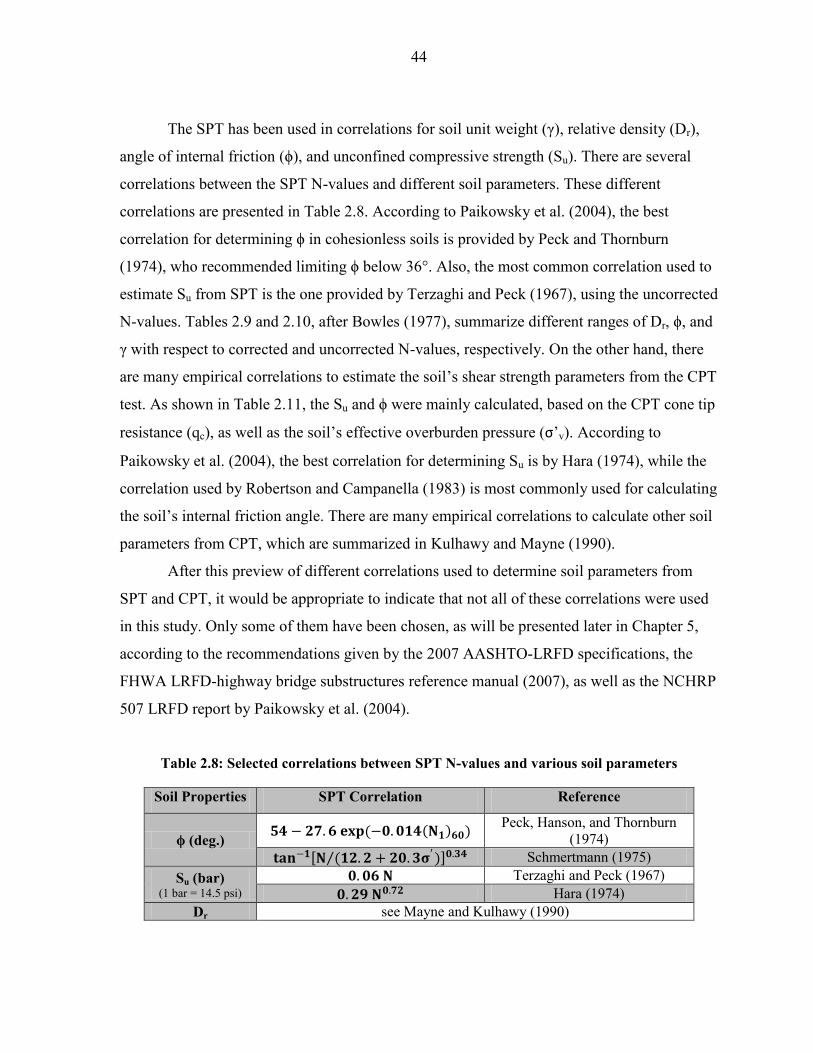
44

The SPT has been used in correlations for soil unit weight (γ), relative density (Dr),

angle of internal friction (ϕ), and unconfined compressive strength (Su). There are several

correlations between the SPT N-values and different soil parameters. These different

correlations are presented in Table 2.8. According to Paikowsky et al. (2004), the best

correlation for determining ϕ in cohesionless soils is provided by Peck and Thornburn

(1974), who recommended limiting ϕ below 36°. Also, the most common correlation used to

estimate Su from SPT is the one provided by Terzaghi and Peck (1967), using the uncorrected

N-values. Tables 2.9 and 2.10, after Bowles (1977), summarize different ranges of Dr, ϕ, and

γ with respect to corrected and uncorrected N-values, respectively. On the other hand, there

are many empirical correlations to estimate the soil‘s shear strength parameters from the CPT

test. As shown in Table 2.11, the Su and ϕ were mainly calculated, based on the CPT cone tip

resistance (qc), as well as the soil‘s effective overburden pressure (σ‘v). According to

Paikowsky et al. (2004), the best correlation for determining Su is by Hara (1974), while the

correlation used by Robertson and Campanella (1983) is most commonly used for calculating

the soil‘s internal friction angle. There are many empirical correlations to calculate other soil

parameters from CPT, which are summarized in Kulhawy and Mayne (1990).

After this preview of different correlations used to determine soil parameters from

SPT and CPT, it would be appropriate to indicate that not all of these correlations were used

in this study. Only some of them have been chosen, as will be presented later in Chapter 5,

according to the recommendations given by the 2007 AASHTO-LRFD specifications, the

FHWA LRFD-highway bridge substructures reference manual (2007), as well as the NCHRP

507 LRFD report by Paikowsky et al. (2004).

Table 2.8: Selected correlations between SPT N-values and various soil parameters

Soil Properties SPT Correlation Reference

ϕ (deg.) 𝟓𝟒 − 𝟐𝟕.𝟔 𝐞𝐱𝐩(−𝟎.𝟎𝟏𝟒 𝐍𝟏 𝟔𝟎)

Peck, Hanson, and Thornburn

(1974)

𝐭𝐚𝐧−𝟏 𝐍 (𝟏𝟐.𝟐 + 𝟐𝟎.𝟑𝛔′) 𝟎.𝟑𝟒 Schmertmann (1975)

Su (bar) (1 bar = 14.5 psi)

𝟎.𝟎𝟔 𝐍 Terzaghi and Peck (1967)

𝟎.𝟐𝟗 𝐍𝟎.𝟕𝟐 Hara (1974)

Dr see Mayne and Kulhawy (1990)

45

Table 2.9: Dr, ϕ, and γ corresponding to corrected SPT N-values (after Bowles, 1977)

Description Very

Loose Loose Medium Dense Very Dense

Relative density, Dr 0 – 0.15 0.15 – 0.35 0.35 – 0.65 0.65 – 0.85 0.85 – 1.00

Corrected SPT N-

value 0 to 4 4 to 10 10 to 30 30 to 50 50+

Internal friction

Angle, ϕ 25 – 30

o 27 – 32

o 30 – 35

o 35 – 40

o 38 – 43

o

Unit weight, γ

(kN/m3)

(1 kN/m3 = 6.24 pcf)

11.0 – 15.7 14.1 – 18.1 17.3 – 20.4 17.3 – 22.0 20.4 – 23.6

*Use 5% larger values for granular material.

Table 2.10: Ranges of qu and γ with respect to un-corrected SPT (after Bowles, 1977)

Description Very soft Soft Medium Stiff Very Stiff Hard

Su (kPa) (1 kPa = 0.145 psi)

0 – 24 24 – 48 48 – 96 96 – 192 192 – 384 384+

Un-corrected

SPT N-value 0 to 2 2 to 4 4 to 8 8 to 16 16 – 32 32+

γ (kN/m3)

(1 kN/m3 = 6.24

pcf)

15.8 –

18.8 15.8 – 18.8

17.3 –

20.4

18.8 –

22.0 18.8– 22.0

18.8 –

22.0

*Correlations should be used for preliminary estimates only

Table 2.11: Correlations between CPT and soil parameters

Soil

Properties CPT Correlation Reference

ϕ (deg.) 0.1 + 0.38 ∗ log(qc σ′ ) Robertson and Campanella (1983)

Su (bars) (1 bar = 14.5 psi)

(qc − σo)/Nk Hara (1974)

2.7.2. Pile capacity in cohesive soils

Different static methods have been designed empirically or semi-empirically, based

on a reasonable agreement with pile load tests. Some of these methods were based on field

tests conducted in cohesive soils (i.e., clayey soils), restricting their usage to designs in

similar soil types. There are several of these methods, such as the Alpha (α) method, Beta (β)

method, Lambda (λ) method, and CPT-method. On the other hand, there are static methods

46

developed, based on field tests performed in cohesionless soils (i.e., sandy soils). Among

these methods are the SPT-method and Nordlund‘s method. Not all the available static

methods in the literature are presented in this Chapter, but only the most commonly used

methods and the methods that have been recommended for the design of pile foundations by

the 2007 AASHTO-LRFD specifications, the FHWA LRFD-highway bridge substructures

reference manual (2007), as well as the NCHRP 507 LRFD report by Paikowsky et al., 2004.

Before using static analysis methods, geotechnical engineers should be familiar with

the limitations of each method and should be able to choose the appropriate method that best

represents specific soil-pile conditions. Moreover, static methods should not be the only

approach used for designing deep foundations, but several verification techniques should be

performed regularly to check the design. Many state DOTs have developed their own static

analysis methods that better represent their unique soil conditions and construction practices.

Such locally developed methods are generally called the ―In-house‖ method. In 1989, the

Iowa DOT developed its foundation soils information chart for pile foundation after Dirks

and Kam (1989), revised in 1994. The Iowa design charts were given the name ―Bluebook‖

(some time referred to as ―BB‖). In summary, the BB is an in-house static analysis approach,

especially developed for Iowa soils and mainly combines different static analysis methods

together to enhance pile capacity predictions. In the next sections, different static analysis

methods, as well as the BB method, are briefly described.

2.7.2.1 The α-API Method

The α-method (API-1974) is a semi-empirical approach of calculating the pile skin

friction, based on the total stresses induced in the soil and calculated using the soil‘s

undrained shear strength (Su). This method was mainly developed for cohesive or clay soils.

It has been used for many years and has proven to provide reasonable design capacities for

displacement and non-displacement piles. This method depends on the alpha factor (α),

which is indirectly related to the soil‘s undrained shear strength (Su). The factor was back-

calculated from several pile load tests. The main equation used for calculating the pile unit

shaft resistance is as follows:

fs = α . Su [2.31]

47

where,

fs =Unit side-friction resistance.

α =Adhesion factor.

Su =Undrained shear strength in soil adjacent to the foundation.

There are numerous functions that have been developed to correlate the α-value to

different soil properties and pile types. Among the most commonly used functions are those

developed by Tomlinson (1957), Peck (1958), the American Petroleum Institute (API-1974),

and Tomlinson (1980). Figure 2.6 presents some of the different correlations used to

calculate α after Vesic (1977). It is clear from the figure there is a large scatter among the α-

values, which requires local experience while selecting the suitable function used in the

design of piles. According to Coduto (2001), although the API (1974) function was mainly

developed for the design of offshore piles, it is probably the most suitable for the design of

driven piles. The equations used to determine α-values based on the API are as follows:

For; Su < 25 kPa (500 psf):

α = 1 [2.32]

For; 25 kPa (500 psf) < Su< 75 kPa (1500 psf):

α = 1.0 − 0.5 Su−25 kPa

50 kPa (S.I. units) [2.33]

α = 1.0 − 0.5 Su−500 lb /ft2

1000 lb /ft2 (English units) [2.34]

For; Su > 75 kPa (1500 psf):

α = 0.5 [2.35]

On the other hand, O‘Neill and Reese (1999) have developed a bearing capacity

factor (Nc) to calculate the end-bearing resistance of deep foundations in cohesive soil, based

on the soil‘s total undrained shear strength as follows:

q′t

= Nc∗ . Su [2.36]

where,

q′t =Net unit end-bearing resistance.

Su =Undrained shear strength of the soil between pile tip and 2B below the tip.

48

B =Pile diameter.

Nc∗ =Bearing capacity factor (after O‘Neill and Reese, 1999).

= 6.5 if Su ≤ 25 kPa (500 psf) [2.37]

= 8.0 at 25 < Su < 100 kPa (1000 psf) [2.38]

= 9.0 at Su ≥ 100 kPa (2000 psf) [2.39]

Figure 2.6: Measured values of α as back calculated from full-scale static load tests compared

with several proposed functions for α (After Coduto, 2001)

As previously indicated, Su was calculated, based on the correlation to the

uncorrected SPT N-values provided by Terzaghi and Peck (1967). This raised many

arguments against the reliability of the α-method, even if Su was determined, based on

laboratory testing, as the soil sampling method can cause significant disturbance to the soil‘s

properties (Jardine et al., 2005). They added that in the case of driven piles, the driving

process itself could lead to significant changes in soil properties, such as remolding of the

soil next to the pile. This may directly affect the calculated pile skin-friction, based on the α-

method. However, the method has been widely used in practice, as it still provides relatively

reasonable pile capacities in cohesive soils (Coduto, 2001).

Undrained Shear Strength, Su (lb/ft2)

Su (kPa)

α

49

2.7.2.2 The α-Tomlinson Method

Among the common functions developed to correlate the α-value to the soil‘s

undrained shear strength is that developed by Tomlinson (1980). The α-Tomlinson method

has been widely used, especially in stiff clays. This method accounts for different pile

materials (i.e., concrete, timber, or steel piles) and provides reasonable capacity estimates for

large displacement piles; hence, it may not be the most suitable method for driven piles. The

method relies on the α-values, which, in-turn, depend on the bearing embedment in stiff clay

and the width of the pile. The equation used for calculating skin friction using α -Tomlinson

is similar to α-API. The only difference is in the value of α. The equation used is as follows:

fs = α . Su [2.40]

where,


α =Adhesion factor (Figures 2.7 and 2.8 after Tomlinson 1979 and 1980, respectively).

Su =Undrained shear strength in soil adjacent to the foundation.

The same equations mentioned before with the α-API method are used to calculate the end-

bearing resistance of the pile.

2.7.2.3 The β-Method

The β-method (Burland, 1973) is a semi-empirical approach, based on effective

stresses calculated from the vertical effective overburden stress. This method was developed

to model the long-term drainage shear strength. It can be used for different soil types, such as

clay, silt, sand, or gravel, and can even be used for layered soil profiles. According to

Fellenius (1991), the beta factor (β) is affected by soil type, mineralogy, density, strength,

pile installation technique, as well as other factors. The values of β range between 0.23 and

0.8, but cannot exceed 2 for over consolidated soils, as suggested by Esrig and Kirby (1979).

The β-method has been found to work best for piles in normally consolidated and lightly over

consolidated soils. However, the method tends to overestimate pile capacity for heavily over

consolidated soils (AASHTO-interim 2006). The β-method equation for calculating the unit

skin friction is as follows:

fs = β . P o [2.41]

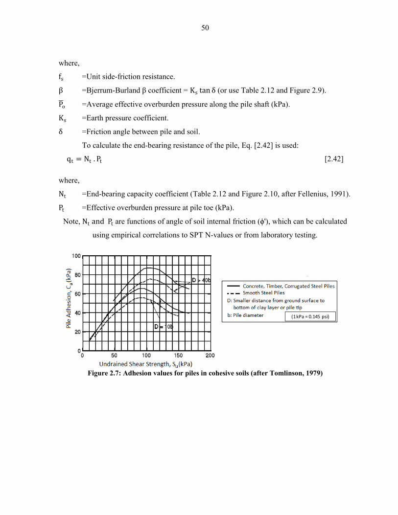
50

where,


β =Bjerrum-Burland β coefficient = Ks tan δ (or use Table 2.12 and Figure 2.9).

P o =Average effective overburden pressure along the pile shaft (kPa).

Ks =Earth pressure coefficient.

δ =Friction angle between pile and soil.

To calculate the end-bearing resistance of the pile, Eq. [2.42] is used:

qt = Nt . Pt [2.42]

where,

Nt =End-bearing capacity coefficient (Table 2.12 and Figure 2.10, after Fellenius, 1991).

Pt =Effective overburden pressure at pile toe (kPa).

Note, Nt and Pt are functions of angle of soil internal friction (ϕ'), which can be calculated

using empirical correlations to SPT N-values or from laboratory testing.

Figure 2.7: Adhesion values for piles in cohesive soils (after Tomlinson, 1979)

(1 kPa = 0.145 psi)

(1 kPa = 0.145 psi)

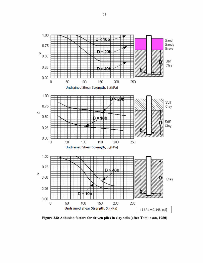
51

Figure 2.8: Adhesion factors for driven piles in clay soils (after Tomlinson, 1980)

(1 kPa = 0.145 psi)

52

Figure 2.9: The β coefficient versus soil type using ϕ' angle (after Fellenius, 1991)

Figure 2.10: The Nt coefficient versus soil type using ϕ' angle (after Fellenius, 1991)

β

ϕ (degrees)

Nt

ϕ (degrees)

53

Table 2.12: Approximate range of β and Nt coefficients (after Fellenius, 1991)

Soil type ϕ' (deg.) β Nt

Clay 25 – 30 0.23 – 0.40 3 – 30

Silt 28 – 34 0.27 – 0.50 20 – 40

Sand 32 – 40 0.30 – 0.60 30 – 150

Gravel 35 – 45 0.35 – 0.80 60 – 300

2.7.2.4 The λ-Method

The λ-method (Corps of Engineers, 1992) is an empirical approach, based on

effective stresses induced in the soil (calculated from the vertical effective overburden stress)

and total soil strength (calculated from undrained shear strength). This method may be used

to relate the unit skin friction to the passive earth pressure (AASHTO-interim, 2006). The

value of λ was empirically-determined by examining the results obtained from various load

tests conducted on steel pipe piles in cohesive soils. Therefore, this method is more accurate,

if used for the same soil and pile conditions. Eq. [2.43] is used to calculate the skin friction:

qs = λ(ζv′ + 2Su) [2.43]

where,

σv′ + 2Su =Passive lateral earth pressure (ksf).

σv′ =Effective vertical stress at midpoint of soil layer under consideration (ksf).

Su =Undrained shear strength of soil (ksf).

λ =Empirical coefficient (see Figure 2.11 after Vijayvergiya and Focht, 1972).

To calculate the end-bearing resistance of the pile in cohesive soil, the same equations

for the α-method previously mentioned can be used (based on O‘Neill and Reese, 1999).

54

Figure 2.11: Chart for λ factor using pile penetration length (after Vijayvergiya, 1972)

2.7.2.5 The CPT-Method

Nottingham and Schmertmann (1975) developed an empirical approach to calculate

pile capacity, based on the CPT applied to cohesive and cohesionless soils. Correlations to

CPT provide accurate pile design capacities, especially with driven piles. Moreover, it

provides continuous readings for the soil‘s profile and accordingly can take into

consideration the effects of different soil layers. The cone tip resistance (qc) is used to

determine the end-bearing resistance of piles, while the sleeve friction (fs) is used to

determine the skin friction resistance along the shaft. The ultimate shaft resistance in

cohesionless soils can be calculated using the following expression:

Rs = K 1

2 (f s As )0 to 8b + (f s As )8b to D [2.44]

If f s is not available, the shaft resistance in cohesionless soils could be determined

from the cone tip resistance as follows:

Rs = Cf qc x As [2.45]

0

10

20

30

40

50

60

70

0 0.1 0.2 0.3 0.4 0.5

Pil

e P

enet

rati

on

(m

)

λ

(1m = 3.28 ft)

55

In the case of cohesive soils, the shaft resistance could be determined using the

following expression:

Rs = α′ x f s x As [2.46]

where,

𝐾 =Ratio of unit pile shaft resistance to unit cone sleeve friction in sands (Figure 2.12).

𝐷 =Embedded pile length.

b =Pile width or diameter.

f s =Average unit sleeve friction from CPT at the point considered.

As =Pile-soil surface area at the point considered.

Cf =Factor obtained from Table 2.12 after the FHWA-LRFD reference manual, 2007).

𝑞𝑐 =Average cone tip resistance along the pile length.

α′ =Ratio of pile shaft to sleeve friction (use Figure 2.13, after Schmertmann, 1978).

The ultimate tip resistance (or pile end-bearing) shall be determined as follows:

qt =qc 1+qc 2

2 [2.47]

where,

qc1 =Average of cone tip resistance over distance xb following the path 1-2-3 using the

minimum path rule in the upward direction (Figure 2.14, after Schmertmann, 1978).

b =Pile diameter.

x =Value from 0.7 to 4.0 below pile tip as shown on Figure 2.14.

qc2: =Average of cone tip resistance over distance 8b following the path 3-4 using the

minimum path rule as shown on Figure 2.14.

56

Figure 2.12: Penetrometer design curve for side friction in sand (after FHWA, 2007)

Table 2.13: Representative CPT Cf values (after FHWA, 2007)

Type of piles Cf

Precast concrete 0.012

Timber 0.018

Steel displacement 0.012

Open end steel pipe 0.008

Figure 2.13: Design curve for skin-friction in clays by Schmertmann (1978)

(1 kPa = 0.145 psi)

57

Figure 2.14: Procedure suggested for estimating the pile end-bearing capacity by Nottingham

and Schmertman (1975)

2.7.3. Pile capacity in cohesionless soils

2.7.3.1 SPT-Meyerhof Method

The SPT-Meyerhof method (Meyerhof, 1976/1981) is an empirical approach for

calculating the pile capacity, based on SPT tests conducted in cohesionless soils like sands

and non-plastic silts. According to the FHWA-LRFD reference manual (2007), the SPT

method should be only used for preliminary estimates for pile capacity, not for final design

recommendations. This is due to the non-reproducibility of SPT N-values and simplified

assumptions contained in the method. Meyerhof (1976) reported different correlations and

provided some limitations on shaft and tip resistance, according to pile type (displacement or

non-displacement pile). The end-bearing capacity, based on the SPT-Meyerhof method for

piles driven to a depth Db in cohesionless soil, is calculated using the following:

qt =40 N b

′ .Db

b≤ 400N b

′ (kPa) [2.48]

qt =0.8 N b

′ .Db

b≤ N b

′ (ksf) [2.49]

qc1: Average q over a distance xb below the pile tip (path 1-2-3). Sum qc values in both the downwards (path 1-2) and the upward (path 2-3) direction. Use actual qc values along path 1-2 and the minimum path rule along path 2-3. Compute qc1 for x-values from 0.7 to 3.75 below the pile tip and use the minimum qc1 value obtained.

qc2: Average q over a distance 8b above the pile tip (path 3-4) using the minimum path rule.

D: Pile embedded length

Dep

th

qc

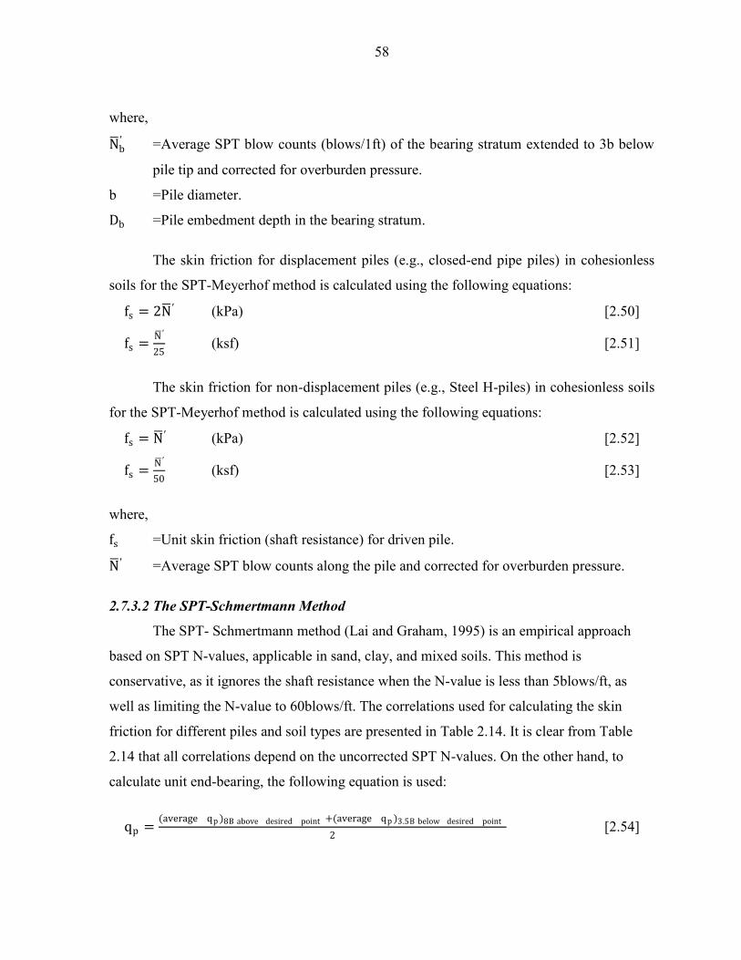
58

where,

N b′ =Average SPT blow counts (blows/1ft) of the bearing stratum extended to 3b below

pile tip and corrected for overburden pressure.

b =Pile diameter.

Db =Pile embedment depth in the bearing stratum.

The skin friction for displacement piles (e.g., closed-end pipe piles) in cohesionless

soils for the SPT-Meyerhof method is calculated using the following equations:

fs = 2N ′ (kPa) [2.50]

fs =N ′

25 (ksf) [2.51]

The skin friction for non-displacement piles (e.g., Steel H-piles) in cohesionless soils

for the SPT-Meyerhof method is calculated using the following equations:

fs = N ′ (kPa) [2.52]

fs =N ′

50 (ksf) [2.53]

where,

fs =Unit skin friction (shaft resistance) for driven pile.

N ′ =Average SPT blow counts along the pile and corrected for overburden pressure.

2.7.3.2 The SPT-Schmertmann Method

The SPT- Schmertmann method (Lai and Graham, 1995) is an empirical approach

based on SPT N-values, applicable in sand, clay, and mixed soils. This method is

conservative, as it ignores the shaft resistance when the N-value is less than 5blows/ft, as

well as limiting the N-value to 60blows/ft. The correlations used for calculating the skin

friction for different piles and soil types are presented in Table 2.14. It is clear from Table

2.14 that all correlations depend on the uncorrected SPT N-values. On the other hand, to

calculate unit end-bearing, the following equation is used:

qp =(average qp )8B above desired point +(average qp )3.5B below desired point

2 [2.54]

59

where,

qp =Weighted average tip resistance from Table 2.15.

B =Pile diameter.

The ultimate tip resistance is fully mobilized, if the actual bearing embedment length

(DA) is equal to the critical bearing embedment length (DC). DC is determined in Table 2.16.

In the case for DA < DC, the mobilized tip resistance for H-piles is reduced. To calculate the

exact reduction in tip resistance, the following equations are used:

If DA< DC and end-bearing soil layer are stronger than the overlying layer, then:

qp = qLC +DA

DC(qT − qLC ) [2.55]

CSFBL = SFBL

qT qLC +

DA

2DC(qT − qLC ) [2.56]

where,

qp =Reduced tip resistance.

qT =Unit tip resistance at layer change.

qLC =Uncorrected unit tip resistance at pile tip.

CSFBL =Reduced side resistance in bearing layer.

SFBL =Uncorrected side resistance in bearing layer.

If DA> DC and end-bearing soil layer are stronger than the overlying layer, then:

CSFACD = USFACD

qCD qLC + 0.5(qCD − qLC ) [2.57]

where,

CSFACD =Corrected side resistance between the top of the layer and the critical depth.

USFACD =Uncorrected side resistance from the top of the bearing layer to critical depth.

qCD =Unit tip resistance at critical depth.

60

Table 2.14: Side resistance correlations for the SPT-Schmertmann method

Type Soil

Description

Ultimate unit shaft resistance qp (tsf)

Concrete piles Steel H-piles Pipe piles

1 Clay 2.0N(110-N)

/4006.6

2N(110-

N)/5335.94 0.949+0.238lnN

2 Mixed soil 2.0N(100-N)

/4583.3

-0.0227+0.033N-

(4.57610-1

)N2+

2.465(E-6*N3)

0.243+0.147lnN

3 Sands 0.019N 0.0116N 0.058+0.152lnN

4 Limestone 0.01N 0.0076N 0.018+0.134lnN

Table 2.15: Tip resistance correlations for the SPT-Schmertmann method

Type Soil

Description

Ultimate unit tip resistance qp (tsf)

Concrete and

Steel H-piles Pipe piles

1 Clay 0.7N 0.48N

2 Mixed soil 1.6N 0.96N

3 Sands 3.2N 1.312N

4 Limestone 3.6N 1.92N

Table 2.16: Critical bearing depth ratio for the SPT-Schmertmann method

Type Soil Description Critical depth

ratio (Dc/B)

1 Clay 2

2 Mixed soil 4

3

Sands (𝐍 ≤ 𝟏𝟐) 6

Sands (𝐍 ≤ 𝟑𝟎) 9

Sands (𝐍 > 30) 12

4 Limestone 6

2.7.3.3 The Nordlund Method

The SPT-Nordlund method (Nordlund and Thurman, 1963) is a semi-empirical

approach based on field observations from pile static load tests. It accounts for different pile

shapes (i.e., constant diameter or tapered piles), as well as pile materials and types, including

steel H-piles, closed and open end pipe piles, and timber piles. According to Hannigan et al.

(2005), this method is preferred in cohesionless soils, such as sandy and gravel soils, as the

pile load tests used to develop the Nordlund‘s design curves were conducted in sandy soils.

61

Moreover, the load tests were conducted for piles with diameters (widths) less than 500 mm

(19.6 inch), which means the method over predicts the capacity for piles with widths larger

than 500 mm (19.6 inch). A detailed pile design procedure using the Nordlund method is

provided in the FHWA design and construction manual (1997). In the case of tapered piles,

the total ultimate pile capacity (shaft resistance and end-bearing) for the Nordlund method is

calculated using the following equation:

Qu = Kδd=Dd=0 . Cf . Pd .

sin (δ+ω)

cos ωCd .∆d + αt . Nq

′ . At . Pt . [2.58]

In the case of piles with uniform cross sections, the capacity is calculated as follows:

Qu = Kδ . Cf . Pd . sinδ . Cd . D + αt . Nq′ . At . Pt [2.59]

The previous equation can also be written as:

Qu = Kδ . Cf . Pd . sinδ . Cd . D + qL . At [2.60]

where,

d =Depth.

D =Embedded pile length.

Kδ =Coefficient of lateral earth pressure at depth d (Tables 2.17 and 2.18).

Cf =Correction factor for Kδ when δ ≠ ϕ (use Figure 2.15).

Pd =Effective overburden pressure at the center of depth increment d.

δ =Friction angle between soil and pile.

ω =Angle of pile taper from vertical.

Cd =Pile perimeter at depth d.

∆d =Length of pile segment.

αt =Factor depending on the pile slenderness ratio (use Figure 2.16).

Nq′ =Bearing capacity factor (use Figure 2.17).

At =Pile toe area.

Pt =Effective overburden pressure at pile toe ≤ 150 kPa (3.2 ksf).

qL =Limiting unit tip resistance (use Figure 2.18).

62

Figure 2.15: Correction factor CF for Kδ when δ ≠ ϕ (after Nordlund, 1979)

Figure 2.16: Chart for estimating the αf coefficient from ϕ (after Nordlund, 1979)

ϕ (degrees)

CF

αt

ϕ (degrees)

63

Table 2.17: Kδ for piles when ω = 0o and V= 0.0093 to 0.093 m

3/m

ϕ Displaced Volume (V), m

3/m

0.01 0.02 0.03 0.04 0.05 0.06 0.07 0.07 0.08 0.09

25 0.70 0.75 0.77 0.79 0.80 0.82 0.83 0.84 0.84 0.85

26 0.73 0.78 0.82 0.84 0.86 0.87 0.88 0.89 0.90 0.91

27 0.76 0.82 0.86 0.89 0.91 0.92 0.94 0.95 0.96 0.97

28 0.79 0.86 0.90 0.93 0.96 0.98 0.99 1.01 1.02 1.03

29 0.82 0.90 0.95 0.98 1.01 1.03 1.05 1.06 1.08 1.09

30 0.85 0.94 0.99 1.03 1.06 1.08 1.10 1.12 1.14 1.15

31 0.91 1.02 1.08 1.13 1.16 1.19 1.21 1.24 1.25 1.27

32 0.97 1.10 1.17 1.22 1.26 1.30 1.32 1.35 1.37 1.39

33 1.03 1.17 1.26 1.32 1.37 1.40 1.44 1.46 1.49 1.51

34 1.09 1.25 1.35 1.42 1.47 1.51 1.55 1.58 1.61 1.63

35 1.15 1.33 1.44 1.51 1.57 1.62 1.66 1.69 1.72 1.75

36 1.26 1.48 1.61 1.71 1.78 1.84 1.89 1.93 1.97 2.00

37 1.37 1.63 1.79 1.90 1.99 2.05 2.11 2.16 2.21 2.25

38 1.48 1.79 1.97 2.09 2.19 2.27 2.34 2.40 2.45 2.50

39 1.59 1.94 2.14 2.29 2.40 2.49 2.57 2.64 2.70 2.75

Table 2.18: Kδ for piles when ω = 0

o and V= 0.093 to 0.93m

3/m

ϕ Displaced Volume (V), m

3/m

0.093 0.186 0.279 0.372 0.465 0.558 0.651 0.744 0.837 0.93

25 0.85 0.9 0.92 0.94 0.95 0.97 0.98 0.99 0.99 1

26 0.91 0.96 1 1.02 1.04 1.05 1.06 1.07 1.08 1.09

27 0.97 1.03 1.07 1.1 1.12 1.13 1.15 1.16 1.17 1.18

28 1.03 1.1 1.14 1.17 1.2 1.22 1.23 1.25 1.26 1.27

29 1.09 1.17 1.22 1.25 1.28 1.3 1.32 1.33 1.35 1.36

30 1.15 1.24 1.29 1.33 1.36 1.38 1.4 1.42 1.44 1.45

31 1.27 1.38 1.44 1.49 1.52 1.55 1.57 1.6 1.61 1.63

32 1.39 1.52 1.59 1.64 1.68 1.72 1.74 1.77 1.79 1.81

33 1.51 1.65 1.74 1.8 1.85 1.88 1.92 1.94 1.97 1.99

34 1.63 1.79 1.89 1.96 2.01 2.05 2.09 2.12 2.15 2.17

35 1.75 1.93 2.04 2.11 2.17 2.22 2.26 2.29 2.32 2.35

36 2 2.22 2.35 2.45 2.52 2.58 2.63 2.67 2.71 2.74

37 2.25 2.51 2.67 2.78 2.87 2.93 2.99 3.04 3.09 3.13

38 2.5 2.81 2.99 3.11 3.11 3.29 3.36 3.42 3.47 3.52

39 2.75 3.1 3.3 3.45 3.45 3.65 3.73 2.8 3.86 3.91

64

Figure 2.17: Chart for estimating the N

’q coefficient from ϕ (after Bowles, 1977)

Figure 2.18: Relationship between the toe resistance and ϕ in sand by Meyerhof (1976)

N’q

ϕ (degrees)

qL

(kP

a)

ϕ (degrees)

(1 kPa = 0.145 psi)

65

2.7.4. Iowa Bluebook method

The Iowa Foundation soils information chart for pile design (or Iowa Bluebook) was

developed in 1989 by Dirks and Kam and revised in 1994. The Bluebook (BB) enables the

design engineer to calculate pile skin friction as well as end-bearing, separately. A

combination of the SPT-Meyerhof method (Meyerhof, 1976/1981) and α-Tomlinson method

(Tomlinson, 1980) were used to develop the pile skin friction design charts for different soil

types. On the other hand, wave equation concepts were used to develop the end-bearing

charts. The BB was calibrated to more than 280 pile load tests, which have been performed in

the state of Iowa since 1968. The BB design chart accounted for different pile materials and

geometry. Practically, the only soil parameter required during the pile design using the BB is

the SPT corrected N-values; hence, it is considered a simple method. The BB has proven to

provide relatively consistent pile designs compared to other complex static analysis methods.

The major limitation of the BB is including an embedded factor of safety equal to 2.0, which

makes it relatively conservative to other design methods and violates the basic principles of

the LRFD approach.

2.7.5. DRIVEN computer program

The DRIVEN computer program was developed by the FHWA in 1998 for

calculating pile capacity. This program calculates the capacity of open and closed end pipe

piles, steel H-piles, concrete piles, and other pile types. From the DRIVEN user manual by

Mathias and Cribbs (1998), the user inputs the soil layer unit weights and strength

parameters, including the percentage strength loss during driving. After selecting the pile

type, the program calculates pile capacity versus depth for cohesive and cohesionless soils.

The methods used for calculating pile capacity in the DRIVEN program are Nordlund

method and α-method (previously described in this chapter) for cohesionless and cohesive

layers, respectively. Several analysis options are included, as the program automatically

subtracts the resistance of unsuitable soil layers and the contribution from scourable soils

from the ultimate pile capacity. Using DRIVEN, the capacity can be calculated at the EOD as

well as BOR with options that account for pile plugging. This program provides a compatible

output data file with the WEAP program to facilitate running drivability studies.

66

2.7.6. SPT-97

SPT-97 is a windows-based computer program developed by FDOT and the

University of Florida. It calculates pile capacity, based on the SPT-Schmertmann method

(Lai and Graham, 1995) described earlier in this chapter. This method was used in the

NCHRP Report 507 (Paikowsky et al., 2004) in LRFD resistance factor calibration.

According to Paikowsky et al. (2004), this computer program proved to provide reasonable

results, except for the two following cases: 1) there is a problem in correcting pile resistance,

when Dc < Da (critical bearing depth is smaller than actual), this problem might occur for

Iowa soils, due to the relatively low Dc (because the main geological formation in the state is

glacial clay with low SPT N-values); and 2) the capacity is incorrectly computed for pipe

piles. This program is available online for geotechnical engineers at the FDOT official

website.

2.7.7. Comparison of different static methods

It is important to compare and select the right static analysis method for a specific

design problem. This should be based on soil and pile types, as well as the extent of available

soil parameters and the degree of accuracy needed from the design. Table 2.19 summarizes

the most commonly used static analysis methods and provides a brief description of the

approach used to derive each method, the recommended soil type, design parameters, and in-

situ tests needed, as well as the advantages and limitations corresponding to different

methods. Table 2.20 summarizes the required equations for calculating the shaft and tip

resistances, using different static analysis methods, and clearly indicates the appropriate soil

type recommended for each method, as well as the required soil parameters or in-situ tests

required for the analysis.

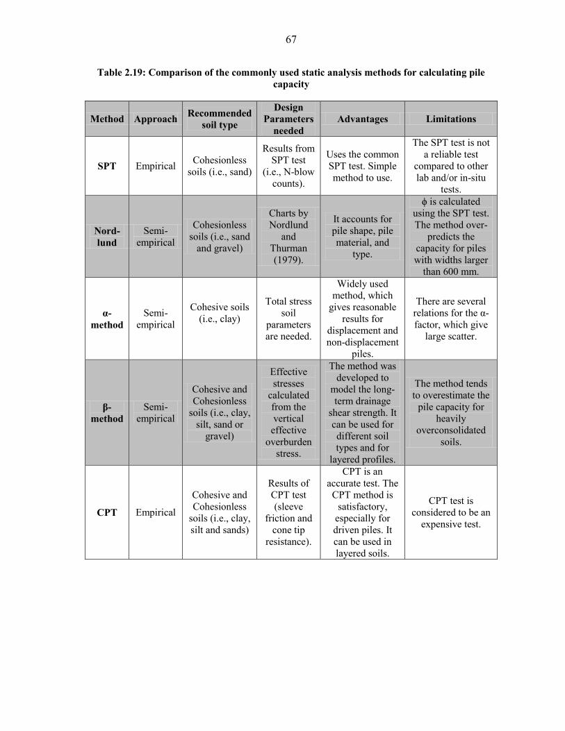
67

Table 2.19: Comparison of the commonly used static analysis methods for calculating pile

capacity

Method Approach Recommended

soil type

Design

Parameters

needed

Advantages Limitations

SPT Empirical Cohesionless

soils (i.e., sand)

Results from

SPT test

(i.e., N-blow

counts).

Uses the common

SPT test. Simple

method to use.

The SPT test is not

a reliable test

compared to other

lab and/or in-situ

tests.

Nord-

lund

Semi-

empirical

Cohesionless

soils (i.e., sand

and gravel)

Charts by

Nordlund

and

Thurman

(1979).

It accounts for

pile shape, pile

material, and

type.

ϕ is calculated

using the SPT test.

The method over-

predicts the

capacity for piles

with widths larger

than 600 mm.

α-

method

Semi-

empirical

Cohesive soils

(i.e., clay)

Total stress

soil

parameters

are needed.

Widely used

method, which

gives reasonable

results for

displacement and

non-displacement

piles.

There are several

relations for the α-

factor, which give

large scatter.

β-

method

Semi-

empirical

Cohesive and

Cohesionless

soils (i.e., clay,

silt, sand or

gravel)

Effective

stresses

calculated

from the

vertical

effective

overburden

stress.

The method was

developed to

model the long-

term drainage

shear strength. It

can be used for

different soil

types and for

layered profiles.

The method tends

to overestimate the

pile capacity for

heavily

overconsolidated

soils.

CPT Empirical

Cohesive and

Cohesionless

soils (i.e., clay,

silt and sands)

Results of

CPT test

(sleeve

friction and

cone tip

resistance).

CPT is an

accurate test. The

CPT method is

satisfactory,

especially for

driven piles. It

can be used in

layered soils.

CPT test is

considered to be an

expensive test.

68

Table 2.20: Summary of the equations required for different static methods

Soil Type Method Shaft Resistance Tip Resistance Required Soil

Parameters

Cohesive

α-API (API-

1974)

fs = α . Su

If: Su ≤ 25 kPa

qt = 6.5 Su

If: 25 < Su < 100 kPa

qt = 8.0 Su

If: Su ≥ 100 kPa

qt = 9.0 Su

Su (undrained

shear strength)

α-Tomlinson

(Tomlinson,

1980)

Su; Db (pile

embedment)

λ- Method (US

Army Corps of

Engineers,

1992)

fs = λ(ζv′ + 2Su)

Su; γ (soil unit

weight)

Cohesive/

Cohesion-

less

β-Method

(Burland,

1973) fs = β . P o qt = Nt . Pt ϕ; γ

CPT-Method

(Nottingham

and

Schmertmann,

1975)

fs

= K 1

2 (f s As )0 to 8b

+ (f s As )8b to D

qt =qc1 + qc2

2 CPT; Db

Cohesion-

less

SPT-Meyerhof

Method

(Meyerhof,

1976/1981)

fs =N ′

25

(ksf)

qt =0.8 N b

′ . Db

b≤ N b

′

(ksf)

SPT; Db

SPT-

Schmertmann

Method (Lai

and Graham,

1995)

fs = f(N)

(see section 2.7.3.2) qt = f(N) SPT

Nordlund

Method

(Nordlund and

Thurman,

1963)

qto tal = Kδ. Cf . Pd . sinδ . Cd . D + αt . Nq′ . At . Pt ϕ; γ; Db

In-house

for

cohesive/

cohesion-

less

Iowa Bluebook

Method (Dirks

and Kam,

1989)

Use the revised design charts for different soil

and pile types SPT

69

2.8. Pile Static Load Test

Static Load Tests (SLTs) accurately measure the actual behavior of pile foundations

in the field when subjected to axial vertical compressive loading and characterize the load-

settlement relationship at the pile head. Load testing is the most definitive method of

determining the nominal capacity of a pile, which provides valuable information to the

design engineer and is recommended for design verification purposes. SLTs can also assist in

calibrating sophisticated design models, such as finite element models, ensuring these models

provide safe results, and eliminating excess conservatism. In difficult soil and bedrock

conditions, the SLT results are the only means of identifying the actual pile capacity. SLTs

can also help generating databases for advanced research.

2.8.1. SLT methods and procedures

There are several SLT methods, procedures, and equipment used for routine pile

testing and proof-testing purposes described in the ASTM D-1143 standards (ASTM, 2007).

Among the different methods are the Slow Maintained Testing Method (SM) and the Quick

Maintained Testing Method (QM). According to the Canadian Foundation Engineering

Manual (1985), the ST method is time consuming and can lead to complex SLT data

evaluation and interpretation. Also, the SM test could affect the pile true load movement

behavior during testing. Conversely, the QM test is faster, more efficient in determining the

pile capacity, and provides accurate results. Therefore, this method is preferable to the SM

method.

Acceptance of the pile SLT is generally governed by building codes reviewed by

structural and geotechnical engineers. The structural engineer determines the maximum

deflection that a structure can sustain without losing its function, while the geotechnical

engineer determines the pile bearing capacity and limits the soil-pile resistance to a certain

extent, such that the deformations do not exceed the plastic behavior. There are several

methods for determining the ultimate pile capacity from a SLT, which can be called the SLT

acceptance criteria. The commonly used acceptance criteria are briefly described in the

following sections.

70

2.8.2. Acceptance criteria

As previously described, the static load test is the most accurate test that represents

the actual response of the piles. Hence, it is vital to select a suitable method of determining

the pile nominal (maximum non-factored) capacity from the load-displacement curve. There

are several methods for determining the nominal pile capacity from a SLT. These methods

have advantages, limitations, and applications, which should be addressed. Some of these

methods are represented in this section because they are the most commonly used, according

to design codes.

2.8.2.1 Davisson’s Method

The Davisson‘s criterion (Davisson, 1972) is one of the most popular methods and

seems to work best with data from the QM test (Coduto, 2001). The criterion is applied by

drawing a parallel line to the elastic compression line (base line) offset by a specified amount

of displacement, depending on the pile size. This parallel line is then called the Davisson

line. As can be seen in Figure 2.19, the point of intersection between the Davisson line and

the load displacement curve is considered the pile nominal capacity. Equation [2.61] is used

to plot the base line on the load-displacement curve:

∆=Qva .L

AE [2.61]

where,

∆ =Elastic movement of base line.

Qva =Applied load.

A =Cross sectional area of pile.

E =Modulus of elasticity of pile material.

L =Embedded length of pile.

To draw the Davisson line parallel to the base line, the following expression is used:

X = 0.15 +D

120 [2.62]

71

where,

X =Offsite displacement from the base line (inch).

D =Pile diameter (inch).

Davisson‘ criterion was originally recommended for different types of driven piles

(Prakash et al., 1990). In the NCHRP report-507 by Paikowsky et al. (2004), different

methods of determining the pile capacity from the load-displacement curve were used and

compared with the static-cyclic capacity of 75 piles. Paikowsky et al. (2004) indicted that the

distribution of the ratio between the capacities determined using Davisson‘s criterion and the

static-cyclic test yielded the closest mean to unity and the least standard deviation compared

to the distributions using other determination methods. Thus, the Davisson criterion was the

only method that was selected to determining the pile nominal capacity from the load-

displacement curve in the NCHRP report-507. One of the main advantages of Davisson‘s

criterion is being an objective method that can be used as an acceptance criterion for the

static load test, as the Davisson parallel line can be predicted even before starting the test.

However, Hannigan et al. (2005) indicated that this method has some limitations, as it under-

predicts pile capacity for piles with diameters larger than 24 inches. Table 2.21 provides a

comparison between Davisson‘s method and other determination methods, presenting the

appropriate pile types for each method, the recommended static load test type, advantages,

limitations, and applicability.

2.8.2.2 Shape of Curvature Method

As shown in Figure 2.20, the nominal pile capacity in the shape of the curvature

method (Butler and Hoy, 1977) can be defined as the point of intersection between the elastic

compression line and the line tangent to the plastic portion of the load-displacement curve.

According to Prakash et al. (1990), this method is applicable for QM tests. The disadvantage

of this method is that it penalizes long piles because they will have larger elastic movements;

hence, it underestimates the capacity of longer piles. Table 2.21 provides a comparison

between the shape of curvature method and other determination methods.

72

Figure 2.19: Determining the pile capacity using Davisson’s method

Figure 2.20: Determining the pile capacity using the shape of curvature

2.8.2.3 Limited Total Settlement Method

The pile capacity can be limited at a point where the settlement of the pile is the

smallest of 0.1 times the pile diameter or 1 inch. This method is an objective method. It could

be used as an acceptance criterion for the static load test, as the limited total settlement line

can be predicted even before starting the test. Also, this method is simple and does not

require any sophisticated equations. However, the method is not suitable for long piles, as

elastic settlement exceeds the limit without inducing plastic deformations. Additionally, the

Load (ton)

Set

tlem

ent

(in

ch)

(1 ton = 2.204 kips)

Load (ton)

Set

tlem

ent

(in

ch)

(1 ton = 2.204 kips)

73

pile may fail before reaching the settlement limit of the method. Figure 2.21 provides an

example of using the limited total settlement method. Table 2.21 provides a comparison

between the limited settlement method and other methods.

Figure 2.21: Determining the pile capacity using the limited total displacement

2.8.2.4 De Beer’s Method

In the De Beer‘s Method (adapted from Bowles, 1996), the load test data is plotted in

a log-log scale, at which the intersection between the two straight portions of the graph will

be equal to De Beer‘s capacity as shown in Figure 2.22. This method was originally proposed

for SM tests (Prakash et al., 1990). One of the most common problems with this method is

the two straight portions in the graph cannot be clearly determined. Table 2.21 provides a

comparison between De Beer‘s method and other determination methods.

0

1

2

3

4

5

0 50 100 150 200 250

Set

tlem

ent

(inch

)Load (kips)

Limited Settlement Line

74

Figure 2.22: An Example of determining the pile capacity using De Beer’s method

2.8.2.5 Chin’s Method

In Chin‘s method (Chin 1970/1971) shown in Figure 2.23, a straight line between

∆/Qva and ∆ is plotted where ∆ is the displacement and Qva is the corresponding load. Then,

the Qult is equal to 1/C1, where C1 is explained in the figure. Chin‘s method was developed

for both QM and SM tests. However, it has several disadvantages. It assumes the load-

moment curve is approximately hyperbolic. Also, Chin‘s method requires constant time

increments used when conducting the SLT. Moreover, a problem could occur while selecting

the straight line passing through the points shown in the figure, as sometimes the points do

not appear to fall in a straight line. This could occur unless the test has passed Davisson‘s

failure criterion. According to Prakash et al. (1990), this method may not provide good

results for static load tests performed according to the ASTM standards, as the tests may not

have exactly constant time load increments.

Load

(k

N)

Settlement (mm)

(1 kN = 0.2248 kips)(1 mm = 0.0394 inch)

75

Figure 2.23: Determining the capacity using Chin’s method (after Prakash et al., 1990)

2.8.2.6 Iowa DOT Method

The Iowa Foundation Pile Design Chart (Dirks and Kam, 1989) was developed, based

on determining the pile actual failure load, using the Louisiana method. The Louisiana

method is defined as the intersection between the tangent of the linear portion of the load-

displacement curve and a line with a slope of 0.05 inches per ton at the yield point. The yield

point is defined as the intersection between the load-displacement curve and a parallel line to

the recovery line at 0.25 inches settlement. This method was essentially adapted for

Louisiana soils and is not frequently used in general geotechnical practices. Moreover, the

method is relatively sophisticated and not recommended by any design codes for the LRFD

calibration. On the other hand, Davisson‘s criterion is an uncomplicated method that has

proven to perform better in the case of driven steel H-piles and was recommended for a

consistent LRFD calibration framework by AASHTO and NCHRP.

0

0.001

0.002

0.003

0.004

0.005

0.006

0.007

0.000 0.050 0.100 0.150 0.200 0.250

Δ/Q

va

(in

/to

n)

.

Movement (in)

76

Table 2.21: Comparison between pile ultimate capacity determination methods including

appropriate pile types for each method, recommended static load test type, advantages,

limitations, and applicability for each method

Method Recommended

pile types

SLT(1)

type Advantages Limitations Comments

Shape of

Curvature

(Fuller

and Hoy,

1977)

Bored, belled,

and small

diameter driven

concrete piles

as well as

Franki piles.

QM(2)

test

It yields

failure loads

near to

actual test

failure

loads.

It is a subjective

method; hence,

results could greatly

vary from one to

other.

Easy method. It

is a conservative

method not

suitable for long

piles.

Davisson’s

(1972)

Driven piles as

well as Franki

piles.

QM

test

An

objective

method,

which can

be used as a

SLT

acceptance.

For piles with

diameters more than

24 inches, this

method under-

predicts the

capacity.

Easy method. A

conservative

method

(recommended

by

specifications).

Chin’s

(1970-

1971)

N/A

QM

and

SM(3)

tests

N/A

Constant time load

increments required

for accuracy. Also,

assumes hyperbolic

load-settlement

relation. Gives

failure loads higher

than that of actual

test failure loads.

Easy method.

Loads must be

higher than

those of

Davisson‘s

acceptance load.

De Beer’s

(1967-

1972)

N/A SM

tests N/A Subjective method.

Moderate

method. Drawn

on log scale.

Hansen’s

90

(1963)

Small diameter

driven concrete

piles.

CRP(4)

tests N/A Trial and error.

Moderate

method

Hansen’s

80

(1963)

N/A

QM

and

SM

tests

Criteria

agree well

with

plunging

failure.

Not suitable for

tests that include

unloading cycles or

unachieved

plunging.

Moderate

method.

Assumes that the

load-

displacement

curve is

parabolic.

Limited

Total

Settlement

N/A N/A Objective

method

Not suitable for

long piles. as elastic

settlement exceeds

limit without

inducing plastic

deformations.

Easy method.

Pile may fail

before reaching

settlement limit

of the method.

(1) Static load test type;

(2) QM: Quick Maintained test2;

(3) SM: Slow Maintained test; and

(4) CRP: Constant

Rate of Penetration Test.

77

2.9. References

AASHTO LRFD Bridge and Construction Specifications (1994). Washington, DC.

AASHTO LRFD Bridge Design Specifications (2004). Washington, DC

AASHTO LRFD Bridge Design Specifications (2006). Washington, D.C.


edition

(2008 Interim), American Association of State Highway Transportation Officials,

Washington, D.C.

AbdelSalam, S. S., Sritharan, S., and Suleiman, M. T. (2008). ―Current design and

construction practices of bridge pile foundations.‖ Proceeding: The International

Foundations Congress and Equipment Expo, March 2009, Orlando, Florida.

Abu-Hejleh, N., DiMaggio, J., and Kramer, W. (2009). ―AASHTO Load and Resistance


Research Board 88th

Annual Meeting, 2009, Paper #09-1034, Washington DC.

Allen, T. M., Nowak, A. S., and Bathurst, R. J. (2005). ―Calibration to Determine Load and

Resistance Factors for Geotechnical and Structural Design.‖ Transportation Research

Circular Number E-C079, TRB, Washington, DC, 83p.

Allen, T. M. (2005). ―Development of the WSDOT Pile Driving Formula and Its Calibration

and Resistance Factor Design (LRFD).‖ FHWA Report, WA-RD 610.1, Washington

State Department of Transportation.

American Concrete Institute (1974). ―Recommendations for Timber Piles Design,

Manufacture and Installation of Concrete Piles,‖ ACI Report No. 543R-74.

Argo, D. E. (1987). ―Dynamic Formulas to Predict Driven Pile Capacity.‖ Department of

Civil and Environmental Engineering, Washington State University, Pullman, WA.

ASTM D1143 (2007). ―Standard Test Methods for Deep Foundations under Static Axial

Compressive Load.‖ American Society for Testing and Materials, ASTM,

Philadelphia, PA.

Baecher, G. (2001). ―Contribution to a progress research report as part of Project NCHRP

24-17, LRFD Deep Foundations Design.‖ unpublished document.

Barker, R., Duncan, J., Rojiani, K., Ooi, P., Tan, C., and Kim, S. (1991). ―NCHRP Report

343: Manuals for the Design of Bridge Foundations.‖ TRB, National Research

78

Council, Washington, D.C.

Becker, D. E. and Devata, M. (2005). ―Implementation and Application Issues of Load and

Resistance Factor Design (LRFD) for Deep Foundations.‖ ASCE Conf. Proc. 156, 1

(2005), DOI:10.1061/40777(156)1

Becker, D. E. (1996). ―Eighteenth Canadian Geotechnical Colloquium: Limit States Design

for Foundations, Part I: An overview of the foundation design process.‖ Canadian

Geotechnical Journal, Vol. 33, No. 6, December, pp. 956–983.

Belcher, D. J., and Flint, R. F. (1946). ―Soil deposits map of United States and Canada.‖

Geological Society of America, Washington, D.C.

Bowles, J. (1977/1996). ―Foundation Analysis and Design.‖ McGraw-Hill, New York.

Broms, B. (1964). ―Lateral Resistance of Piles in Cohesive Soils.‖ Journal of the Soil

Mechanics and Foundations Division, ASCE, Vol. SM2, March, pp. 27–63.

Burland, J. B., (1973). ―Shaft Friction of Piles in Clay.‖ Ground Engineering, London,

Vol.6., No.3, pp.3042.

Butler, H. D., and Hoy, H. E. (1977). ―Users Manual for the Texas Quick-Load Method for

Foundation Load Testing.‖ FHWA-IP- 77-8, FHWA, Office of Development,

Washington, DC.

Canadian Foundation Engineering Manual, (1985). ―Second Edition, Part 3: Deep

Foundations.‖ Canadian Geotechnical Society, BiTech Publishers, Vancouver.

Chang, N. Y. (2006). ―CDOT Foundation Design Practice and LRFD Strategic Plan.‖

Colorado DOT Research Branch, Report No. CDOT-DTD-R-2006-7.

Chellis, R. D. (1949). ―The Relationship Between Pile Formulas and Load Tests.‖ ASCE:

American Society of Civil Engineers, Transactions 114:290-320.

Cheney, R. S. and Chassie, R. G. (1993). ―Soils and Foundations Workshop Manual.‖ FHWA

Report No. FHWA-HI-88-009.

Chin, F. V. (1970). ‗‗Estimation of the Ultimate Load of Piles Not Carried to Failure.‘‘

Proceeding: The 2nd

Southeast Asian Conference on Soil Engineering, pp. 81–90.

Coduto, D. P. (2001). ―Foundation design: principles and practices.‖ Prentice-Hall Inc.,

Englewood Cliffs, N.J.

Cummings, A. E. (1940). ―Dynamic Pile Driving Formulas.‖ Journal of the Boston Society of

79

Civil Engineers, No. 27:6-27.

Davisson, M. (1972). ―High Capacity Piles.‖ Proceeding: Soil Mechanics Lecture Series on

Innovations in Foundation Construction, ASCE, IL Section, Chicago, IL, pp. 81–112.

DiMaggio, J., Saad, T., Allen, T., Barry, R., Al Dimillio, Goble, G., Passe, P., Shike, T., and

Person, G. (1999). ―FHWA International Technology Exchange Program.‖ FHWA

Report Number FHWA-PL-99-013.

Dirks, K. and Kam P. (2003). ―Foundation Soils Information Chart – Pile Foundation.” Iowa

Department of Transportation, Office of Road Design, Ames, Iowa, United States.

Ellingwood, B., Galambos, T. V., Macgregor, J. G., and Cornell, C. A. (1980).

―Development of a Probability Based Load Criterion for American National Standard

A58 - Building code requirements for minimum design loads in buildings and other

structures.‖ National Bureau of Standards, Washington, D.C.

Esrig, M. I., and Kirby, R. C. (1979). ―Soil Capacity for Supporting Deep Foundation

Members in Clay.‖ ASTM, STP. No. 670, pp. 27–63.

Fellenius, B. H., (1991). ―Summary of Pile Capacity Predictions and Comparison with

Observed Behavior.‖ ASCE: American Society of Civil Engineers, ASCE, Journal of

Geotechnical Engineering, Vol. 117, No. 1, pp. 192 - 195.

FHWA (1997). ―Design and Construction of Driven Pile Foundations.‖ Workshop manual,

Volumes I, publication FHWA-HI-97-013.

FHWA (2007). ―Load and Resistance Factor Design (LRFD) for Highway Bridge

Superstructures.‖ FHWA Publication number: FHWA-NHI-07-034

Foye, K. C., Abou-Jaoude, G., Prezzi, M., and Salgado, R. (2009). ―Resistance Factors in

Load and Resistance Factor Design of Driven Pipe Piles in Sand.‖ Journal of

Geotechnical and Geoenvironmental Engineering, ASCE, v 135, n 1, 2009, p 1-13.

Fragaszy, Richard J., Douglas E., Argo, and Higgins, J. D. (1989). ―Comparison of Formula

Predictions with Pile Load Tests.‖ Transportation Research Record: Journal of the

Transportation Research Board, TRR 1219:1-12.

Gates, M. (1957). ―Empirical Formula for Predicting Pile Bearing Capacity.‖ Civil

Engineering, 65-66.

Gibbs, H. J. and Holtz, W. G. (1957). ―Research on Determining the Density of Sands by

80

Spoon Penetration Testing.‖ Proc. of the 4th

Int. conference of Soil Mechanics and

Foundation Engineering, London 1,35-39.

Green, R. (1994). ―LRFD Code for Ontario Bridge Substructures.‖ Transportation Research

Record, ISSN 0361-1981, 1994, no1447, pp. 73-79.

GRL, Inc. (1999). ―Pile-Driving Analyzer, PAK Users Manual.‖ Goble, Rausche, Likins and

Associates, 1999.

Gulhati, Sahashi, K., and Manoj, D. (2005). ―Geotechnical Engineering.‖ New Delhi,

Haryana India: Tata McGraw-Hill Publishing Company Limited.

Hannigan, P. J., Goble, G. G., Thendean, G., Likins, G. E., and Rausche, F. (2005). ―Design

and Construction of Driven Pile Foundations.‖ Vol. I and II, Federal Highway

Administration Report No. FHWA-HI-05, Federal Highway Administration,

Washington, D.C.

Hannigan, P. J., Goble, G. G., Thendean, G., Likins, G. E., and Rausche, F. (1998). ―Design

and Construction of Driven Pile Foundations.‖ Volumes I and II, FHWA-HI-97-013.

National Highway Institute, Federal Highway Administration, U.S. Department of

Transportation, Washington, D.C. in Geotechnical Load and Resistance Factor

Design.‖ Journal of Geotechnical and Geoenvironmental Eng., Vol. 129, No. 4, April

2003, pp. 287-295.

Hansen, J. B. (1963). ―Hyperbolic Stress-strain Response: Cohesive Soils,‖ Discussion

Journal of the Soil Mechanics and Foundations Division, American Society of Civil

Engineers, New York, NY, Vol. 89, No. SM4.

Hara, A., Ohta, T., Niwa, M., Tanaka, S., and Banno, T. (1974). ―Shear Modulus and Shear

Strength of Cohesive Soils.‖ Soils and Foundations, Vol. 14, No. 3, Sept. 1974.

Iowa DOT (2008). ―Standard Specifications with GS-01014 Revisions.‖ Iowa DOT

Electronic Reference Library, http://www.erl.dot.state.ia.us/Apr_2008/GS/frame.htm.

Iowa DOT LRFD Design Manual (2009). ―Office Policies and Procedures, Office of Bridges

and Structures.‖ Iowa DOT Electronic Reference Library.

Jardine R. J, Chow, F. C, Overy, R., and Standing, J. (2005). ―ICP Design Methods for

Driven Piles in Sands and Clays.‖ Publishers Thomas Telford Inc.

Kerkhoff, G. O., Oehler, L. T., and Housel, W. S. (1965). ―A Performance Investigation of

http://cedb.asce.org/cgi/WWWdisplay.cgi?0880014

81

Pile Driving Hammers and Piles.‖ Lansing, Michigan State Highway Commission.

Kulhawy, F., and Phoon, K. (1996). ―Engineering Judgment in the Evolution from

Deterministic to Reliability-Based Foundation Design.‖ Proceeding: The 1996

Conference on Uncertainty in the Geologic Environment, UNCERTAINTY’96. Part 1

(of 2), July 31–Aug. 31, Madison, WI, ASCE, NY, pp. 29–48.

Kulhawy, F. H. and Mayne, P. W., (1990). ―Manual on Estimating Soil Properties for

Foundation Design.‖ Report. EL-6800, Electric Power Research Ins., Palo Alto.

Kuo, C. L., McVay, M. C., and M., Birgisson, B. (2002). ―Calibration of Load and

Resistance Factor Design: Resistance factors for drilled shaft design.‖ Transportation

Research Record ISSN 0361-1981, 2002, no 1808, pp. 108-111.

Kyung, K. J., Gabr, M. A., and Shamimur, M. R. (2002). ―Development of Resistance

Factors for Axial Capacity of Driven Piles in North Carolina.‖ PhD Dissertation,

North Carolina State University, Raleigh, North Carolina, October, 2002.

Lai, P., and Graham, K. (1995). ―Static Pile Bearing Analysis Program.‖ SPT94:

http://www.dot.state.fl.us/structures/manuals/spt94.zip.

Lai, P., McVay, M., Bloomquist, D., and Badri, D. (2008). ―Axial Pile Capacity of Large

Diameter Cylinder Piles.‖ Proceeding: From Research to Practice in Geotechnical

Engineering Congress, 2008.

Mathias D., and M. Cribbs (1998). ―DRIVEN 1.0: A Microsoft Windows Based Program for

Determining Ultimate Static Pile Capacity.‖ Federal Highway Administration.

McVay, M., Birgisson, B., Zhang, L., Perez., A, and Putcha, S. (2000). ―Load and Resistance

Factor Design (LRFD) for Driven Piles Using Dynamic Methods - A Florida

Perspective.‖ Geotechnical Testing Journal, Vol. 23, No. 1, pp. 55–66.

McVay, M., Klammler, H., Bloomquist, D., Otero, J., and Farone, M. (2010). ―Modification

of LRFD Resistance Factors Based on Site Variability.‖ NTIS website, accessed

March 2010.

Mertz, D. R. (2007). ―AASHTO-LRFD Background to the Specifications.‖ Aspire,

Precast/Prestressed Concrete Institute.

Meyerhof, G. (1970). ―Safety Factors in Soil Mechanics.‖ Canadian Geotechnical Journal,

Vol. 7, No. 4, pp. 349–355.

http://www.dot.state.fl.us/structures/manuals/spt94.zip

http://www.engineeringvillage2.org/controller/servlet/Controller?CID=quickSearchCitationFormat&searchWord1=%7bMcVay%2C+Michael%7d&section1=AU&database=1&yearselect=yearrange&sort=yr

http://www.engineeringvillage2.org/controller/servlet/Controller?CID=quickSearchCitationFormat&searchWord1=%7bBadri%2C+Dhuruva%7d&section1=AU&database=1&yearselect=yearrange&sort=yr

82

Meyerhof, G. (1976). ―Bearing Capacity and Settlement of Pile Foundations.‖ ASCE:

American Society of Civil Engineers, Journal of the Geotechnical Engineering

Division, Vol. 102, No. 3, March, pp. 195–228.

Misra, A. and Roberts, L. A. (2006). ―Probabilistic Analysis of Drilled Shaft Service Limit

State Using the t-z Method.‖ Canadian Geotechnical Journal, 1324-1332 (2006).

Misra, A., Roberts, L. A. and Levorson, S. M. (2007). ―Reliability of Drilled Shaft Behavior

using Finite Difference method and Monte Carlo simulation.‖ Geotechnical and

Geological Engineering, no.25, 65-77.

Moore, J. (2004/2005). ―AASHTO LRFD Oversight Committee (OC) survey 2004 and the

Update 2005.‖ New Hampshire DOT, AASHTO Load and Resistance Factor Design

(LRFD) Bridge Specifications information website, accessed May, 2008.

Moore, J. (2007). ―AASHTO LRFD Oversight Committee (OC) Update 2007.‖ New


Specifications information website, accessed May, 2008.

Nordlund, R. L. (1963/1979). ―Bearing Capacity of Piles in Cohesionless Soils.‖ Journal of

Soil Mechanics and Foundation Engineering, JSMFE, Vol. 89, SM 3, pp 1-36.

Nottingham, L., and Schmertmann, J. (1975). ―An Investigation of Pile Capacity Design

Procedures.‖ Final Report D-629 to Florida Department of Transportation,

Department of Civil Engineering, University of Florida, pp 159.

Nowak A. S. and Collins K. R. (2000). ―Reliability of Structures.‖ Publisher: McGraw-hill.

Nowak, A. S. (1999). ―NCHRP Report 368: Calibration of LRFD Bridge Design Code.‖

TRB, Washington, DC.

Olson, R. E., and Flaate, K. S. (1967). ―Pile-Driving Formulas for Friction Piles in Sand.‖

ASCE Journal of Soil Mechanics and Foundation Division 93 (No. SM 6):279-296.

O'Neill, M. W. and Reese, L. C. (1999). ―Drilled Shafts: Construction Procedures and Design

Methods.‖ FHWA Report No. IF-99-025, Federal Highway Administration,

Washington, D.C.



M. (2004). ―Load and Resistance Factor Design (LRFD) for Deep Foundations.‖

83

NCHRP Report, no. 507, TRB, Washington D.C.

Passe, P. (1997). ―Florida‘s Move to the AASHTO LRFD Code.‖ STGEC 97, Chattanooga.

Tennessee.

Peck, R. B., W. E. Hanson, and T. H. Thornburn (1974). ―Foundation Engineering.‖ John

Wiley & Sons, pp. 514.

Pile Dynamics, Inc. (2000). ―CAPWAP for Windows Manual.‖ Cleveland, Ohio: Pile

Dynamics, Inc.

Prakash, S., and Sharma, H. D. (1990). ―Pile Foundations in Engineering Practice.‖ Wiley,

New York.

Ramey, G. E., and Hudgins, A. P. (1975). ―Modification of Pile Capacity and Length

Prediction Equations Based on Historical Alabama Pile Test Data.‖ Montgomery,

AL: State of Alabama Highway Department - Bureau of Research and Development.

Rausche, F., and Goble, G. (1979). ―Determination of Pile Damage by Top Measurements.‖

ASTM: American Society for Testing and Materials, Philadelphia, PA


Methodology for Service Limit State Design of Deep Foundations using t-z Model

Approach.‖ Proceeding: The Geo-Congress 2008, New Orleans, LA.

Robertson, P. K., and Campanella, R. G. (1983). ―Interpretation of Cone Penetration Tests.‖

Canadian Geotechnical Journal, Vol. 20, No. 4, Nov. 1983.

Schmertmann, J. H. (1975). ―Measurement of in-situ Shear Strength, State-of-the-art

Report.‖ Proceeding: The American Society of Civil Engineers Conference on In Situ

Measurements of Soil Properties, Raleigh, North Carolina, 2, 57–138.

Schmertmann, J. H. (1978). ―Guidelines for Cone Penetration Test, Performance and

Design.‖ FHWA Report No. FHWA-TS-78-209, U.S. DOT, Washington, D.C.

Scott, B., Kim, B. and Salgado, R. (2003). ―Evaluation of Load Factors for Use in

Geotechnical Design.‖ Journal of Geotechnical and Geoenvironmental Engineering,

ASCE, 129(4), 287-295.

Skempton, A.W. (1951), ―The Bearing Capacity of Clays.‖ Proc. Building Research

Congress, vol. 1, pp. 180-189.

Tang, W. (1993). ―Recent Developments in Geotechnical Reliability.‖ Proceeding: The

http://www.cpt-robertson.com/pdfs/Interpretationofcptrobcamp.pdf

84

Conference on Probabilistic Methods in Geotechnical Engineering.

Terzaghi, K., and Peck, R. B. (1967). ―Soil Mechanics in Engineering Practice.‖ Wiley.

Thibodeau, E., and Paikowsky, S. (2005). ―Performance Evaluation of a Large Scale Pile

Load Testing Program in Light of Newly Developed LRFD Parameters.‖ Proceeding:

Session of the Geo-Frontiers 2005 Congress, January 24-26, 2005, Austin, Texas.

Tomlinson, M. J. (1957). ―The Adhesion of Piles Driven in Clay Soils.‖ Proceeding: The 4th

International Conference on Soil Mechanics and Foundation Engineering, Vol. 2,

1957, pp. 66-71, Butterworth Scientific Publications, Ltd. London, England.

Tomlinson, M. J. (1980/1995). ―Foundation Design and Construction.‖ 6th

Edition. Longman

Scientific & Technical, Essex, England.

U.S. Army Corps of Engineers, (1992). ―Pile Layout to Minimize Interference.‖ Engineer

Technical Letter ETL 1110-8-17(FR), Department of the Army, US Army Corps of

Engineers, Washington, DC, 20314-1000.

VanderVeen, C. (1953). ―The Bearing Capacity of a Pile.‖ Proceeding: The 3rd

International

Conference on Soil Mechanics and Foundation Engineering, Vol. 2.

Vesic, A. S. (1977). ―Design of Pile Foundations.‖ National Cooperative Highway Research

Program Synthesis of Highway Practice No. 42, Transportation Research Board,

Washington, D.C.

Vijayvergiya, V. N., and Focht, J. A. (1972). ―A New Way to Predict Capacity of Piles in

Clay.‖ Proceeding: The 4th

Annual Offshore Technology Conference, Houston, TX,

Offshore Technology.

Withiam, J. L., Voytko, E. P., Barker, R. M., Duncan, J. M., Kelly, B. C., Musser, S. C., and

Elias, V. (1998). ―Load and Resistance Design LRFD for Highway Bridge

Substructures.‖ Federal Highway Administration, Washington, D.C.

85

CHAPTER 3: CURRENT DESIGN AND CONSTRUCTION PRACTICES OF

BRIDGE PILE FOUNDATIONS WITH EMPHASIS ON LRFD IMPLEMENTATION

Sherif S. AbdelSalam1; Sri Sritharan, M. ASCE

2; Muhannad T. Suleiman, M. ASCE

3

A paper accepted for publication in the Journal of Bridge Engineering, ASCE

3.1. Abstract

The Federal Highway Administration mandated the use of the Load and Resistance

Factor Design (LRFD) approach in the U.S. for all new bridges initiated after September

2007. This paper presents bridge deep foundation practices established through a nationwide

survey of more than 30 state Departments of Transportation (DOTs) from 2008. Highlighted

by this study are the benefits of the LRFD, as well as how its flexibility is exploited in design

practice. This study collected information on current foundation practices, pile analysis and

design, pile drivability, pile design verification, and quality control. Since this is the first

nationwide study conducted on the LRFD topic following the FHWA mandate, the status on

the implementation of LRFD for bridge foundation design was also examined. This study

determined: 1) more than 50% of the responded DOTs use the LRFD for pile design, while

30% are still in transition to the LRFD; and 2) about 30% of the DOTs, who use the LRFD

for pile foundations, utilizes regionally-calibrated resistance factors to reduce foundation

costs.

CE Database keywords: LRFD, Implementation, Survey, Bridge, Deep Foundations, Pile

Analysis, and Design.

1 Graduate Student and Research Assistant, Dept. of Civil, Construction, and Environmental

Engineering, Iowa State University, 355 Town Engineering, Ames, IA 50011-3232, E-mail:[email protected] 2 Wilson Engineering Professor and Associate Chair, Dept. of Civil, Construction and Environmental

Engineering, Iowa State University, 376 Town Engineering, Ames, IA 50011-3232, E-mail: [email protected] 3Assistant Professor, Dept. of Civil and Environmental Engineering, 321 Acopian Engineering Center,

Lafayette College, Easton, PA, 18042. E-mail: [email protected]






86

3.2. Introduction

It has long been recognized that standard bridge design specifications, based on the

allowable (or working) stress design (ASD) approach, do not promote a consistent reliability

for design; thus, they fail to ensure uniform levels of performance for bridges. Since the mid-

1980s, the Load and Resistance Factor Design (LRFD) approach has been progressively

developed with the objective of ensuring a uniform reliability for bridges. In LRFD

specifications, the targeted reliability index (β) defines the measure of safety associated with

a probability of failure (Pf) in a limited range of 3 to 3.6 for different types of foundations

(Meyerhof, 1970). According to Barker et al. (1991), a reduced β value in the range between

2.0 to 2.5 could be used for redundant piles, such as those in a pile group. This is because

failure of a pile in a pile group does not necessarily lead to failure of the foundation. For this

reason, Paikowsky et al. (2004) recommended a reliability index of 2.33 (corresponding to a

Pf = 1%) for redundant piles as opposed to a value of 3.00 (corresponding to Pf = 0.1%)

suggested for non-redundant piles. In comparison, the reliability indices corresponding to the

factors of safety (FS) used in the ASD of bridge foundations ranged from 1.5 to 4.7 (Mertz,

2007), indicating a large variation in the probability of failure for this approach.

Although the LRFD approach to designing structural elements has been well

established and implemented in design codes around the world, its application to

geotechnical design has been relatively slow (DiMaggio, 1999). This caused the Federal

Highway Administration (FHWA) to mandate the use of the LRFD approach in the design of

state bridges initiated in the United States after October 1, 2007. Despite the FHWA

mandated deadline, not all State Departments of Transportation (DOTs) have adopted the

LRFD in their foundation designs. This could be due to the potential conservatism of the

LRFD bridge design specifications with a likely anticipation of increase in the foundation

cost. This is more likely the case when resistance factors used in design account for the large

variation in soil parameters, as well as different levels of uncertainty associated with

determining the capacity of deep foundations (Paikowsky et al., 2004). Consequently,

regionally-calibrated resistance factors are permitted in LRFD to minimize the unnecessary

conservatism built into the design, provided these factors are developed in a consistent

manner with the approach suggested in the 2007 LRFD Specifications by the American

87

Association of State Highway and Transportation Officials (AASHTO).

As part of an ongoing research project for the Iowa Highway Research Board (IHRB)

aimed at establishing LRFD resistance factors for the design of deep foundations in the state

of Iowa by accounting for the local soil conditions, a study was conducted through a web-

based survey to determine current design and construction practices of deep foundations

nationwide. In addition to the basic questions relevant to the implementation of the LRFD

methods in bridge foundation design practice, information on design and construction

practices of bridge deep foundations was gathered and analyzed in the following topic areas:

pile analysis and design, pile drivability, pile design verification methods, and quality control

of pile construction.

Two features of this survey are: 1) this was the first survey conducted after the

October 1, 2007 deadline imposed by the FHWA, and 2) it focused on collecting detailed

information on the design and construction practices of bridge deep foundations. The

outcomes of this survey are presented in this paper, which encourage bridge designers to

adopt the LRFD method for pile foundation design and highlight the benefits of utilizing

regionally-calibrated resistance factors.

3.3. Background

With an anticipation of implementing the LRFD methodology to new bridge

foundations in the United States, several questionnaires and surveys have been conducted

over the past decade to monitor the degree of LRFD implementation. In 1999, the FHWA

developed a questionnaire concerning the design and construction practices for deep

foundations and distributed it to State Highway officials, Transportation Research Board

(TRB) representatives, and FHWA geotechnical engineers via the Internet (Paikowsky et al.,

2004). A total of 45 responses were received. According to this survey, 37% of the

respondents used the ASD method for foundation design with a factor of safety ranging from

2.0 to 3.0. Among these respondents, 35% used the AASHTO Load Factor Design (LFD)

method and only 28% used the AASHTO-LRFD method. This survey also collected useful

information about the design and construction considerations for both driven piles and drilled

shafts.

88

In 2004, The AASHTO-LRFD Oversight Committee (OC) conducted a survey among

the State Departments of Transportation (DOTs) to monitor the degree of implementation of

the LRFD approach for bridge substructure design (Moore, 2004), with a follow-up survey in

2005. The committee found that 12 states had fully implemented the LRFD method for

foundation design in 2004 and this number increased to 16 in 2005. In 2006, researchers at

the University of Colorado sent a questionnaire to all state DOTs as part of developing the

LRFD strategic plan for foundation design practice in Colorado (Chang, 2006). Only 28

DOTs responded to the questionnaire, which revealed less than 22% of the respondents had

either implemented or started the implementation of LRFD for bridge foundations, while the

remaining 78% had not even attempted LRFD implementation. In 2007, the AASHTO-

LRFD OC updated the LRFD implementation survey in their progress report (Moore, 2007),

which indicated 44 states would have fully implemented the LRFD approach for all new

bridges by October 1, 2007—the FHWA mandated deadline.

Based on the outcomes of the aforementioned questionnaires and surveys conducted

before the October 1, 2007 deadline, it was observed the focus of past surveys was to

examine the degree of LRFD implementation for foundation design. The construction issues

and/or details of the design procedures adopted for the bridge foundations were not

examined. Consequently, the previous surveys did not provide any information on the use of

regionally-calibrated resistance factors nor did they address the design verification and

quality control practices adopted for pile foundations.

3.4. Data Collection

The data for the study reported in this paper were collected through a web-based

survey developed in January 2008 and distributed to DOT officials from different states as

well as FHWA engineers. A total of 33 completed surveys were received during the first

quarter of 2008.One response was received from the FHWA-Eastern Federal Lands Highway

Division (EFLHD), one from the Alberta Infrastructure & Transportation, Canada, and the

remainder came from 31 different state DOTs. With input from the Iowa DOT officials, the

survey was designed as user-friendly and aimed at gathering information on current design

and construction practices of pile foundations—emphasizing LRFD and ASD design

http://www.efl.fhwa.dot.gov/

http://www.efl.fhwa.dot.gov/

89

approaches. Although nearly 100 questions were included, the survey utilized several logical

branches to minimize the time required to complete the survey; i.e., respondents were not

exposed to questions unrelated to their design and construction practice.

3.5. Goals and Topic Areas

The goal of the survey was to determine the current design and construction practices

of deep foundations nationwide, focusing on the LRFD implementation for bridge

substructure design and the current usage of regionally-calibrated LRFD geotechnical

resistance factors. The survey had four topic areas: 1) foundation practice, 2) pile analysis

and design, 3) pile drivability, and 4) design verification and quality control.

The foundation practice section contained general questions that acquired information

about typical soil formations, average depths to bedrock, routine in-situ and laboratory tests

performed in soil, frequency of using deep foundations for bridges, as well as the types and

sizes of frequently used piles. The pile analysis and design section was next, which included

questions about the use of various design methods, the extent of implementation of the LRFD

method, load and geotechnical resistance factors used in accordance with LRFD, factors of

safety used with the ASD method, and load factors used with the LFD method. Information

about the different analysis methods used to calculate pile capacity (i.e., static methods,

dynamic methods, and dynamic formulas) was also collected.

The third section on pile drivability focused on questions related to soil setup and

relaxation, and their effect on pile capacity in different soil types. Furthermore, this section

gathered information on determining the required pile penetration length during driving and

the definition of pile refusal. The final section on design verification and quality control

obtained information on pile design verification tests conducted during the construction

stage, the frequency of performing the Static Load Test (SLT) on pile foundations, and

different methods used for determining the pile nominal capacity based on SLT. At the end

of the survey, respondents were asked to share information about available SLT databases

and to provide general comments on the survey as well as their contact details.

90

3.6. Major Findings

Presented in this section is a summary of analysis results of responses received from

the 31 state DOTs in the four main topic areas of the survey. In addition, the responses

received from FHWA-EFLHD and Alberta Infrastructure & Transportation are highlighted in

the presentation of results where appropriate.

3.6.1. Foundation practice

Figure 3.1 presents a summary of results obtained for the common foundation

practice in different states. Included in this figure are the most common soil formations;

average depth to bedrock; the most commonly used category of deep foundations, pile types,

and sizes; and the static analysis methods used in pile design. Respondents were allowed to

identify up to three different soil formations for each state. Consequently, the soil formation

shown for each state in Figure 3.1 was based on survey responses. For a few respondents

who opted not to answer this question and the state DOTs who did not respond to the survey,

the soil formation shown was based on geological maps (Belcher and Flint, 1946).

For questions about commonly used in-situ and laboratory tests used to define soil

parameters, 94% of the respondents reported use of the Standard Penetration Test (SPT),

52% use the Cone Penetration Test (CPT), 16% use the Vane Shear Test (VST), and around

20% perform some other uncommon tests. Note, the respondents were allowed to identify an

unlimited number of tests in this category. Furthermore, all respondents reported performing

basic laboratory soil tests, such as Atterberg limits and soil classification, while 42% stated

they perform triaxial tests, 35% reported performing the unconfined compression test, 29%

perform the direct shear test, and 16% perform some other uncommon laboratory tests.

Despite the subjective nature of the test, the survey confirmed a majority of respondents

depend on SPT tests to determine the basic soil parameters.

The next set of questions gathered information about the use of different foundation

types associated with bridges, the most commonly used categories of deep foundations, as

well as details about the commonly used types of driven piles and drilled shafts. For the

choice of foundation type, about 91% of the respondents indicated they more frequently use

deep foundations than shallow foundations in different soil types, while shallow foundations

91

are used primarily for low volume bridges in shallow bedrock or gravel. Among deep

foundation users, 76% use driven piles, 18% use drilled shafts, and 6% use a combination of

both types. Figures 3.2 and 3.3 highlight the percentage of usage of different types of driven

piles and drilled shafts, respectively. Among the driven pile users, all respondents indicated

they use steel H-piles, while 80% use closed-end pipe piles, 40% use open-end pipe piles,

32% use precast/prestressed concrete piles, 8% use precast concrete piles, 4% use timber

piles, and about 12% of the respondents reported using other pile types (e.g., monotube piles,

tapered tube piles, and a combination of prestressed concrete and steel H-piles).Among the

drilled shaft users, it was determined 83% use cast-in-drilled-hole shafts (CIDH), 50% use

soldier piles, 33% use continuous flight auger (CFA), and 33% use micropiles.

Furthermore, the respondents were asked to identify the most common pile size(s)

they use. This information is included in Figure 3.1, which revealed steel H-piles and

precast/prestressed concrete piles are more commonly used on the East Coast of the United

States, where soil formation is mainly composed of coastal plain and glacial tills. On the

West Coast, where the soil profile is mainly composed of alluvium soil, open-end pipe piles

are more commonly used. Most of the states in the Midwest use steel H-piles, where the main

soil profile is composed of glacial tills. In specific areas of the West, the CIDH shafts are

also widely used, presumably due to the seismic requirements and the possibility of forming

dependable plastic hinges in this foundation type.

The bridge foundation practices reported by FHWA-EFLHD and the Alberta

Infrastructure & Transportation were similar to those of the state DOTs. Both indicated they

depend on SPT and CPT for determining the in-situ soil parameters and they mainly perform

Atterberg limits and the unconfined compression test as the basic laboratory soil tests. The

FHWA-EFLHD indicated they frequently use deep foundations for bridge construction,

especially driven steel H-piles and precast concrete piles. Alberta Infrastructure &

Transportation indicated the usage of the same foundation type for bridge construction, but

with emphasis on driven steel H-piles and open-end pipe piles.

92

3.6.2. Pile analysis and design

The questions for this section were aimed at understanding the deep foundation

design and analysis process practiced by different state agencies. This section began with

questions directed at determining the pile resistance criterion in cohesive and cohesionless

soils. In cohesive soils, it was found 88% of the respondents depend on both skin friction and

end bearing, 6% of the respondents depend only on skin friction, and 6% of them indicated

they ignore end bearing only when the average SPT N-value is less than 12 blows per 30.5

cm (1 ft). In cohesionless soils, it was found 87% of the respondents depend on combining

the resistances obtained through skin friction and end bearing, 9% depend only on skin

friction, and 4% include the resistance from end bearing only when the average SPT N-value

is greater than 25 blows per 30.5 cm (1 ft).

Furthermore, the most preferred method for designing deep foundations was

determined the ASD method, confirmed by 45% of the respondents. The primary reasons for

this choice are their familiarity with the ASD method and possible increase in foundation

cost when the AASHTO-LRFD specifications are used, due to the built-in conservatism.

However, the LRFD approach was reported to be the most commonly used method, due to

the imposed FHWA mandate. About 52% of the survey respondents are currently using

LRFD, while 33% of them are in a transition stage from ASD to LRFD, and about 15% of

respondents are still using ASD with a factor of safety ranging from 2 to 2.5.

Figure 3.4 shows the current extent of LRFD implementation in the design of bridge

foundations in the United States. This figure was created by combining the 31 responses

collected from the state DOTs with the results of the AASHTO-LRFD OC survey (Moore,

2007) to obtain data for the 19 DOTs who did not respond to the recent survey. Even though

the FHWA mandate was implemented in October 2007, 15 state DOTs, who responded to the

survey, and 11 of those, who only responded to the AASHTO-OC survey, are believed to be

either still using the ASD method or in a transition stage to the LRFD approach for designing

bridge foundations. Among the DOTs who responded using the LRFD method for foundation

design, 46% are using regionally-calibrated resistance factors based on SLT database and

reliability theory, 23% are using regionally-calibrated factors by fitting to the ASD factor of

safety, while 31% are using the geotechnical resistance factors as specified in the current

93

AASHTO Specifications (2007). Information on the assumed risk or probability of failure

(Pf) for the LRFD approach to pile foundations was also requested. Since they are currently

not using LRFD or in transition to LRFD, 15 of the respondents did not answer this question.

Another nine respondents reported they were unaware of the assumed probability of failure.

However, four respondents indicated they rely on a Pf value of less than 1/100 for the piles,

while three reported using a Pf value in the range of 1/5000 to 1/1000. Although no specific

question was asked relating the pile redundancy to Pf, the reported variation in Pf is believed

to be due to the assumed redundancy of the piles.

The next set of questions collected information about the different static analysis

methods, dynamic analysis methods, and dynamic formulas used for determining pile

capacity. It was found about 2/3 of the respondents employ a combination of static and

dynamic methods. Respondents, who reported using this combination, essentially deploy the

static analysis methods for determining the number of piles and dynamic analysis methods or

dynamic formulas for finalizing the penetration length.

As shown in Figure 3.5, the most common static analysis method used for piles in

cohesive soils is the α-method at 42% (Tomlinson, 1957; API, 1974). About 32% of the

respondents reported using the β-method (Esrig and Kirby, 1979), 11% use the CPT method

(Nottingham and Schmertmann, 1988), and 9% follow the λ-method (US Army Corps of

Engineers, 1992). Figure 3.5 also reveals the most popular static analysis method for piles in

cohesionless soils is Nordlund‘s method (Nordlund and Thurman, 1963) by 63%. About 40%

of the respondents use the SPT method (Meyerhof, 1976/1981) and 6% use in-house methods

for piles in cohesionless soils. Most of the respondents chose the Nordlund‘s method as the

most accurate static method for sandy soils, and the α-method as the most accurate static

method for clayey soils. Note; the survey permitted multiple answers for this particular set of

questions. Complete descriptions of the different static analysis methods identified above

may be found in Hannigan et al. (1998).

For dynamic analysis methods, all respondents reported using the Wave Equation

Analysis Program (WEAP) for determining pile capacity. The most commonly used software

for this purpose was GRLWEAP (GRL, 1999), where 41% define the soil parameters using

the soil type based method (ST), 28% use the SPT N-values based method (SA), 21% use the

94

Driven software (Hannigan et al., 1998), and 10% follow some other unspecified approaches.

Figure 3.6 represents the use of other dynamic analysis methods—74% of the respondents

indicated they use the Pile Driving Analyzer (PDA) and the CAse Pile Wave Analysis

Program (CAPWAP), while 16% use other uncommon methods. Information collected on the

frequently used dynamic formulas in the design of deep foundations is presented in Figure

3.7. About 57% of the respondents prefer the FHWA-modified Gates formula, 21% use the

ENR formula, 14% use the Gates formula, and more than 43% use in-house formulas.

Complete descriptions of the different dynamic formulas identified above may be found in

Hannigan et al. (1998). More than 80% of the respondents chose the dynamic analysis

methods as more accurate and reliable than static analysis methods and dynamic formulas in

determining the capacity of deep foundations.

In this part of the survey, the different extreme load types used in the design of bridge

foundations, as well as the different methods used for estimating the lateral displacement

demand of piles, were also inquired. For the extreme load consideration, it was found that

37% of the respondents account for scour load in their design, 25% include earthquake load,

20% account for loads due to collision, and 18% use a combination of extreme loads. All

respondents reported lateral displacement is a design consideration for piles. However, the

method used for determining pile displacement demand varied—72% of the respondents use

p-y curves, 14% use the Broms method (Broms, 1964), and 14% use other methods, such as

the FB-Pier strain wedge theory, point of fixity method, and empirical methods. In the

context of lateral demand on piles, it is worth noting the expected pile displacement is

significantly influenced by the abutment type chosen for the bridge. For example, integral

abutments designed without any expansion joints are becoming an increasingly popular

choice among various DOTs. When bridges are designed with integral abutments, the

superstructure loads in the longitudinal and traverse direction may not only be distributed

over more supports, thus increasing the design efficiency of the foundations, but they also

increase the pile redundancy (Mistry 2005).

In general, the FHWA-EFLHD pile design practice was found to be similar to that of

the State DOTs. The FHWA-EFLHD indicated that they are still in a transition stage from

ASD to LRFD and that they are currently using the resistance factors from the 2007

95

AASHTO LRFD Specifications for the LRFD approach. For the design of bridge pile

foundations, they indicated the use of static analysis methods such as α-, β-, and Nordlund.

As for the pile design verification, the FHWA-EFLHD response noted that the use of the

SLT less frequently and the preferred approach being the dynamic analysis methods (i.e.,

PDA and CAPWAP) and dynamic formulas (i.e., ENR, Gates, and FHWA-modified Gates).

A point of contrast between the FHWA-EFLHD bridge foundation design practice and that

of the state DOTs is that FHWA-EFLHD considers the static analysis methods to be more

accurate than the dynamic methods as long as the soil strength parameters are adequately

obtained. On the other hand, the Alberta Infrastructure & Transportation pile design practice

was quite different from that of the state DOTs in that they have already implemented the

LRFD approach for the design of bridge foundations and depend on the Canadian Highway

Bridge Design Code for determining the appropriate LRFD resistance factors. They mainly

use the static analysis methods in the design of bridge deep foundations and the appropriate

static method for a given site is reported to be selected by the consulting firm chosen for the

project. They also indicated to be using the ENR dynamic formula for design verification.

3.6.3. Regionally-calibrated LRFD resistance factors

As previously indicated, among those who have already implemented the LRFD

approach to their design of bridge foundations, 12 DOTs use regionally-calibrated resistance

factors that are more suitable for the local soil types. These resistance factors were calibrated

based on local SLT data and using statistical approaches based on reliability theory. Of the

DOTs, who are still in transition to the LRFD, six of them have adopted preliminary,

regionally-calibrated resistance factors, which were established using their local design and

construction experience as well as the recommended load factors to retain the factor of safety

used for the ASD method. This information, together with details about soil formation, deep

foundation practice, and design methodology is summarized in Table 3.1. Of the respondents,

11 of them indicated that they have a collection of SLT data for their state, as identified in

the table.

Note that the First Order Second Moment (FOSM) and the First Order Reliability

Method (FORM) are two common reliability approaches that can be used for the LRFD

96

calibration. According to Allen et al. (2005), FOSM is the most straightforward technique, in

which the random variables are represented by their first two moments, i.e., the mean (μ) and

standard deviation (ζ), while the Coefficient of Variation (COV) is defined by ζ/μ.

Paikowsky et al. (2004) performed the LRFD calibration for the resistance factors using both

methods and concluded that the difference between them is around 10%, with FOSM

providing slightly conservative resistance factors. Moreover, the 2007 AASHTO-LRFD

specifications are based on the FOSM assuming a lognormal distribution of the load and

resistance density functions. Although specific questions about the selected reliability

approach used for the LRFD calibration were asked, most tend to follow the FOSM approach

because it was used in the 2007 AASHTO-LRFD specifications.

All the reported regionally-calibrated resistance factors for different soil and pile

types were examined using statistical means, in order to establish a representative mean and

standard deviation so that benefits of the reported resistance factors could be realized. The

minimum sample size (N) for these statistical analyses was limited to three. For all datasets,

the mean and standard deviation were determined as a function of the soil type, pile type, and

static analysis method. For those datasets with N < 3, only the average resistance factors

were determined. All of these results are summarized in Tables 3.2 and 3.3. Figure 3.8

presents the histograms and frequency distributions as well as the confidence intervals for the

Probability Density Functions (PDFs) of the reported resistance factors for steel H-piles in

different soil types. As shown in Figure 3.8, the PDFs of different datasets follow a normal

distribution, while the probability of the upper and lower limits of the true mean of each

dataset were found within 95% confidence intervals. As indicated by the standard deviations

in Table 3.2, it appears that the mean of the reported regionally-calibrated resistance factors

for a given soil type are somewhat consistent, especially for the steel H-piles. Also note in

this table that the mean resistance factor of the open-end pipe piles is greater than those

established for the steel H-piles and CIDH shafts. However, it is noted that the resistance

factor of the pipe piles is based only on two data points. For resistance factors reported for

different static analysis methods in Table 3.3, smaller standard deviations are again observed,

indicating smaller variations in the reported resistance factors for a given method and soil

type. Furthermore, it is noted that the in-house methods lead to higher resistance factors than

97

those determined for routinely used static analysis methods.

Table 3.4 compares the mean values of the regionally-calibrated resistance factors

from Tables 3.2 and 3.3 with those reported in the National Corporative Highway Research

Project (NCHRP) report number 507 by Paikowsky et al. (2004) and the 2007 AASHTO-

LRFD Specifications. In most cases, it is observed that the AASHTO recommendations are

more conservative than those proposed by Paikowsky et al. (2004). Furthermore, the mean of

the reported regionally-calibrated resistance factors by different DOTs in all cases are equal

to or greater than the recommended values in NCHRP 507 and the AASHTO Guidelines. In

some cases, the regionally-calibrated factors are twice as high as those recommended for

design practice by AASHTO. Therefore, it is clear that the LRFD regional calibration could

result in higher resistance factors as previously shown, thus optimizing the pile design and

reducing the foundation costs.

The benefits of using regionally-calibrated resistance factors in pile design can be

realized through a simple design example. Consider a bridge pier with a maximum factored

axial load of 8900 kN (2000 kips) that is to be designed with a deep foundation consisting of

18.3 m (60 ft) long steel HP 254 mm (depth) x 62.4 kg/m (self-weight) (10 in. x 42 lbs/ft),

connected with a concrete cap. The soil formation at the site is firm to very firm glacial clay

with silt seams and boulders, with medium soil variability. If the α-API (API, 1974; Coduto,

2001) static analysis method is used for the design of the pile foundation, the axial capacity

of a single pile is 567 kN (127 kips). Using the LRFD resistance factor of 0.35 provided in

the 2007 AASHTO specifications, the design capacity of a single pile is 198.5 kN (42 kips),

requiring a minimum of 45 piles. If the average regionally-calibrated resistance factor of 0.47

for the α-API method is used from Table 3.3, the design capacity of each pile is 266.5 kN (60

kips), needing a total of only 34 piles. This 25% reduction in number of piles will

significantly reduce the foundation cost as it reduces the construction costs of both the piles

and the pile cap.

3.6.4. Pile drivability

In the design stage, the pile penetration length required in the field is estimated using

the chosen static analysis method. However, the penetration length may be readjusted at the

98

construction site using the pile driving data. It was found that 31% of the respondents depend

on a WEAP analysis and field observations to readjust the pile penetration length, 20%

employ dynamic formulas to make the adjustments, and 15% rely on the initial static analysis

results and make no adjustments to pile length in the field (see Figure 3.9). Interestingly, 6%

of the respondents noted that they drive the pile until refusal, while 4% prefer to drive the

piles until the bedrock is reached. The remaining 24% of respondents indicated that they use

a combination of the aforementioned methods depending on the site conditions and design

requirements.

Effects of soil relaxation and setup on the pile capacity were also addressed in this

section of the survey and it was found that more than 50% of the respondents believe that the

pile capacity is unaffected by relaxation in cohesive soils. The responses of those who

indicated that the pile capacity is affected by relaxation were grouped based on the most

predominant soil formation that they indicated for their region. Accordingly, 40% of

respondents noted that the change in pile capacity would not exceed 5% of the value

expected at End of Driving (EOD) in silty sands, 6% indicated that the effect varies from 5 to

10% in sandy soils, and only 2% assumed that the effect exceeds by 20% of the pile capacity

in silts. Similarly, as for the influence of soil setup on the pile capacity, 34% of the

respondents indicated that the pile capacity increases above 20% of the value at EOD due to

setup in clays and silty clays, 25% indicated that the effect varies from 5 to 10% in glacial

tills and clays, 25% indicated that the effect varies from 11 to 20% in clayey silts, 6%

indicated that the soil setup effect does not exceed 5% on the pile capacity, and 10% of the

respondents assume that the pile capacity is unaffected by soil setup in cohesionless soils.

3.6.5. Design verification and quality control

This final section of the survey focused on design verification and quality control

issues. All but one respondent indicated that they perform field tests on 5 to 10% of the

installed piles to verify the design capacity. Among several different techniques, about 45%

of respondents have used the SLT for design verification, while others predominantly use the

dynamic monitoring approach especially for friction piles (i.e., use of WEAP, PDA and

CAPWAP). Usually for small projects, the WEAP analysis is considered as an adequate pile

99

design verification technique, but for large scale projects, the PDA and CAPWAP are

preferred. Among those who use SLT, 73% responded that they use the Davisson‘s criterion

(Davisson, 1972) to define the pile nominal capacity, 26% use the limited total settlement

method, 7% use the shape of curvature method, and 13% follow other unspecified methods.

The most commonly used quality control (QC) tests in the field were found to be:

gamma-gamma test (which is used with drilled shafts installed using the slurry displacement

method), cross hole sonic test, pile verticality measures, and weld/placement inspection.

More than 45% of respondents reported that they perform such QC tests on 5% of installed

piles, another 45% of them perform QC tests less frequently, and the remaining 10% never

perform such tests.

3.7. Conclusions

This paper has presented results from an important survey on the current design and

construction practices of deep foundations for bridges, which is one of the first surveys to be

completed following the FHWA mandate on the use of the LRFD approach in the U.S. on all

new bridges initiated after October 1, 2007. The outcomes of the survey are significant in

that they give an overview of the current bridge foundation practices and highlight how

frequently the state DOTs take advantage of the provision in the AASHTO-LRFD

Specification to improve the deep foundation design by employing regionally-calibrated

geotechnical resistance factors and the associated benefits. Based on the responses received,

the conclusions drawn from the study are as follows:

1. As of June 2008, 52% of the DOTs who responded to the survey have adopted the

LRFD approach for the design of bridge deep foundations, 33% of them were in a

transition phase from ASD to LRFD, and the remaining 15% still followed the ASD

approach with a factor of safety ranging from 2 to 2.5. Of those using the LRFD

method, six DOTs use geotechnical resistance factors by fitting to ASD, eight are

following the 2007 AASHTO-LRFD recommended values, while 12 DOTs have

adapted their own regionally-calibrated factors based on reliability theory.

2. The mean of the reported regionally-calibrated geotechnical LRFD resistance factors

were statistically analyzed and presented in Tables 3.1 through 3.4. The LRFD

100

regionally-calibrated resistance factors reported for sands and clays are either equal to

or greater than the AASHTO recommended values. In sand, the resistance factors are

as much as 50% above those recommended by AASHTO, while values as much as

100% above the recommended values are used for clay. Such large increases in

resistance factors will likely reduce the overall cost of bridge deep foundations.

3. In the design stage, state DOTs are using static analysis methods for determining the

pile capacity. The most commonly used methods in cohesive soils are the α- and β-

methods. On the other hand, the most commonly used static methods in cohesionless

soils are the Nordlund and SPT methods. Most of the respondents chose the α-

method and the Nordlund method to be the most accurate method for determining

the pile capacity in cohesive and cohesionless soils, respectively.

4. During the construction of deep foundations, the DOTs employ either dynamic

analysis methods or dynamic formulas to verify the pile capacity estimated by a static

analysis method. Although all of the respondents noted that they use WEAP as a

dynamic analysis method, 75% indicated that they use a combination of PDA and

CAPWAP in addition to WEAP. Of those who use dynamic formulas for pile

capacity verification, the majority of respondents either use the FHWA-modified

Gates formula or a locally developed formula.

3.8. Acknowledgments

The study reported in this paper was conducted by the authors as part of the ongoing

research project TR-573: Development of LRFD Design Procedures for Bridge Pile

Foundations in Iowa, which is funded by the Iowa Highway Research Board (IHRB). The

authors also express their gratitude to 1) all respondents of the survey; 2) Sandra Larson and

Mark Dunn, Research and Technology Bureau of Iowa DOT, for their coordination and

support of the project; 3) Norm McDonald, State Bridge Engineer for Iowa, for inviting other

DOTs to participate in the survey; and 4) the following members of the project Technical

Advisory Committee for their guidance and advice: Ahmad Abu-Hawash, Dean Bierwagen,

Lyle Brehm, Ken Dunker, Kyle Frame, Steve Megivern, Curtis Monk, Michael Nop, Gary

Novey, John Rasmussen and Bob Stanley. The members of this committee represent Office

101

of Bridges and Structures, Soils, Design Section, and Office of Construction of the Iowa

DOT, FHWA Iowa Division, and Iowa County Engineers.

3.9. References


edition,

2008 Interim, American Association of State Highway and Transportation Officials,

Washington, D.C.

Allen, T. M., Nowak, A.S., and Bathurst, R. J. (2005). ―Calibration to Determine Load and

Resistance Factors for Geotechnical and Structural Design.‖ Transportation Research

Circular Number E-C079, TRB, Washington, DC, 83p.

Barker, R., Duncan, J., Rojiani, K., Ooi, P., Tan, C., and Kim, S. (1991). ―NCHRP Report

343: Manuals for the Design of Bridge Foundations.‖ Transportation Research

Board, National Research Council, Washington, D.C.

Belcher, D.J., and Flint, R. F. (1946). ―Soil Deposits Map of United States and Canada.‖

Geological Society of America, Washington.

Broms, B. (1964). ―Lateral Resistance of Piles in Cohesive Soils.‖ Journal of the Soil

Mechanics and Foundations Division, ASCE, Vol. SM2, March, pp. 27–63.

Chang, N. Y. (2006). ―CDOT Foundation Design Practice and LRFD Strategic Plan.‖

Colorado DOT Research Branch, Report No. CDOT-DTD-R-2006-7


Innovations in Foundation Construction, ASCE, Illinois Section, Chicago, IL, pp.

81–112.

DiMaggio, J., Saad, T., Allen, T., Barry, R., Al Dimillio, Goble, G., Passe, P., Shike, T., and

Person, G. (1999). FHWA International Technology Exchange Program, report

number FHWA-PL-99-013.

GRL, Inc. (1999). ―Pile-Driving Analyzer, PAK Users Manual.‖ Goble, Rausche, Likins, and

Associates.

Hannigan, P.J., Goble, G.G., Thendean, G., Likins, G.E. and Rausche, F. (1998). ―FHWA-

HI-97-013: Design and Construction of Driven Pile Foundations-Volume I and II.‖

National Highway Institute, Federal Highway Administration, U.S. Department of

102

Transportation, Washington, D.C.

Moore, J. (2004/2005). AASHTO LRFD Oversight Committee (OC) survey 2004 and the

Update 2005, New Hampshire DOT, AASHTO - LRFD Bridge Specifications

information website. (http://www.ridot.us/aashto/agenda.htm), accessed May, 2008.

Moore, J. (2007). AASHTO LRFD Oversight Committee (OC) Update 2007, New


Specifications information website (http://www.transportation.org/sites/bridges),

accessed May, 2008.

Mertz, D. R. (2007). ―AASHTO-LRFD Background to the specifications.‖ Aspire,

Precast/Prestressed Concrete Institute.

Meyerhof, G. (1970). ―Safety Factors in Soil Mechanics.‖ Canadian Geotechnical Journal,

Vol. 7, No. 4, pp. 349–355.

Mistry, V. (2005). ―Integral Abutments and Joint-less Bridges,‖ Proceeding: The Integral

Abutment and Joint-less Bridges Conference, FHWA, Baltimore, 3-11.



M. (2004). ―NCHRP Report, 507: Load and Resistance Factor Design (LRFD) for

Deep Foundations.‖ TRB, Washington D.C.

http://www.ridot.us/aashto/agenda.htm

103

Table 3.1: Reported factors sorted according to pile types, static methods, and soil types

State Pile Type Static Analysis Dynamic

Analysis

Dynamic

Formulas

Resistance Factors

Cohesive Cohesionless Sand Clay Mix

CA* Steel H-

piles

CPT-

method Nordlund P + C + W

(1) F-G

(2) 0.45 0.35 N/A

CO CIDH SPT-

method SPT-method P + C + W

ENR, G(3)

, F-

G 0.1 0.9 0.5

CT* Prestressed In-house In-house P + C + W Not used 0.65 0.65 0.65

ID* Steel H-

piles β-method SPT-method P + C + W F-G 0.45 0.45 0.45

MA* Open-pipe In-house Nordlund P + C + W Not used 0.65 0.65 0.65

NH* Closed-

pipe α-method Nordlund P + C + W Not used 0.45 0.35 N/A

NJ* CIDH α-method Nordlund P + C + W Not used 0.45 0.35 0.4

NM* Steel H-

piles β-method Nordlund P + C + W ENR, G, F-G 0.35 0.45 N/A

NV Steel H-

piles α-method Nordlund Not used Not used 0.35 0.25 N/A

PA* Steel H-

piles β-method Nordlund P + C + W Not used 0.5 0.5 0.5

UT* Steel H-

piles α-method Nordlund Not used Not used 0.5 0.7 0.7

WA Steel H-

piles In-house In-house WEAP F-G 0.5 0.5 0.5

WY Steel H-

piles

CPT-

method Nordlund Not used Not used 0.45 0.35 0.35

*Pile Load Test Database available; (1)

P + C + W: PDA, CAPWAP, and WEAP; (2)

F-G: FHWA Modified

Gates method; (3)

G: Gates method.


according to different pile and soil types

Pile Type Reported Factors in Sand

Reported Factors in

Clay

Reported Factors in Mixed

Soils

N(1)

Mean S.D.(2)

N Mean S.D. N Mean S.D.

Steel H-pile 11 0.48 0.11 12 0.48 0.15 8 0.55 0.13

CIDH 4 0.4 0.23 3 0.6 0.28 3 0.5 0.13

Open-end

Pipe 2 0.65 N/A 2 0.67 N/A 2 0.67 N/A

(1) Sample Size; and

(2) Standard Deviation.

104


according to different static analysis methods and soil types

Static

Analysis

Method

Reported Factors in Sand Reported Factors in Clay Reported Factors in Mix

Soil

N Mean S.D. N Mean S.D. N Mean S.D.

Nordlund 11 0.5 0.12 N/A 4 0.53 0.17

SPT

method 3 0.45 0.25 N/A 3 0.53 0.11

α-method N/A 6 0.47 0.19 N/A

β-method N/A 4 0.49 0.13 N/A

CPT

method N/A 3 0.45 0.17 N/A

In-house 3 0.62 0.11 4 0.63 0.10 3 0.62 0.11

Table 3.4: Comparison between the reported resistance factors and the recommended factors in

NCHRP 507 and 2007 AASHTO-LRFD Specifications

Soil Type Static Analysis

Method NCHRP

AASHTO-

Specifications

Mean of Reported

Resistance Factors

Sand

SPT- method 0.45 0.3 0.45

β-method 0.3 N/A 0.65

Nordlund 0.45 0.45 0.5

In-house N/A N/A 0.62

Clay

α-method 0.45 0.35 0.47

β-method 0.2 0.25 0.49

In-house N/A N/A 0.63

105

Figure 3.1: U.S. Map for soil formations, average bedrock depth, commonly used deep

foundation categories, types and sizes, and static methods used in different States

Figure 3.2: Distribution of the most commonly used driven pile types for bridge foundations

`

MT

WY

ID

WA

OR

NV UT

CA

AZ

ND

SD

NE

CO

NM

TX

OK

KS

AR

LA

MO

IA

MN

WI

IL

IN

KY

TN

MS AL GA

FL

SC

NC

VAWV

OH

MI

NY

PA

MD

DE

NJ

CTRI

MA

ME

VTNH

AK

HI

150 m

DS, CIDH,

dia. 1.5 to 3 m

Nord/CPT

15 to 60 m

DP, OEP,

dia. 30 to 50 cm

α/β/Nord

> 45 m

DP, OEP,

dia. 1 to 1.5 m

α/β/Nord

> 15 m

DS, CIDH,

dia. 10 to 30 cm

α/β/Nord/SPT

DP, HP,

α/λ/Nord

DP, OEP,

dia. 40 to 60 cm

10 m

DP, HP,

310x79 mm

α/β/λ/Nord/SPT

Deep

DP and DS

β-method

15 m

DS, CIDH,

SPT

Deep

DP, HP,

360x132 mm

β/SPT

Deep

DS, CIDH,

dia. 1.2 to 3 m

60 m

DP, HP,

360x152 mm

DP, HP,

all sizes

< 15 m

DS, CIDH,

No response

No response

No response No response

No response

No response

Nord/SPT/ In-house

> 25 m

DS, CIDH,

dia. 1 to 1.5 m

α/SPT

Deep

DP, PSCP,

dia.40 to 60cm

α/Nord

No response

20 m

DP, HP,

250x63; 250x85mm

In-house

No response

60 m

DP, HP,

250x63;

360x109 mm

α/Nord

20 m

DP, HP,

250x63,

360x132 mm

In-house

No response

No response

30 m

DP, PSCP,

dia. 0.5 to 1.5 m

In-house

10 m

DP, HP,

310x79;

360x174 mm

PSCP, 30 to 40 cmNord/SPT

> 30 m

DP, PSCP,

30 to 60 cm

< 20 m

DP, HP,

310x79;

360x132 mm

SPT

5 to 60 m

DP, HP,

α/β/Nord

< 15 m

DP, HP,

250x85;

310x110 mm

Nord/SPT

< 15 m

DP, HP,

310x79 mm

Nord< 20 m

DP, CEP,

dia. 30 cm

α/Nord < 15 m

DP, DS,

Nord/SPT/CPT

No response

< 10 m

DP, HP,

250x85; 310x110 mm

α/Nord

Each State contains the following information (if available):

1) Depth to bedrock

2) Used pile categories and types (see map key)

3) Used pile sizes (see map key)

4) Used static analysis methods (see map key)

Map Key

DP = Driven Piles

DS = Drilled Shafts

HP = Steel H-piles

OEP = Open End Pipe piles

CEP = Closed End Pipe piles

CIDH = Cast In Drilled Hole piles

No response

No response

No response

No response

No response

No response

Glacial

Alluvium

Coastal Plain

Other Soil Types

Soil RegionsPSCP = Prestressed Concrete

α = α-method

β = β -method

λ = λ-method

Nord = Nordlund method

SPT = SPT-methods

CPT = CPT-method

100%

80%

40%

32%

8%4%

12%

0%

10%

20%

30%

40%

50%

60%

70%

80%

90%

100%

Steel

H-pilesClosed

End PipeOpen

End Pipe

Pre-

stressed

Precast

Concrete

Other

Types

Timber

Piles

106

Figure 3.3: Distribution of the most commonly used drilled shaft types for bridge foundations

Figure 3.4: Current extent of LRFD implementation

Figure 3.5: Most commonly used static analysis methods for the design of deep foundations

83%

50%

33% 33%

0%

10%

20%

30%

40%

50%

60%

70%

80%

90%

100%

CIDH Soldier piles CFA Micropiles

MT

WY

ID

WA

OR

NV

UT

CA

AZ

ND

SD

NE

CO

NM

TX

OK

KS

AR

LA

MO

IA

MN

WI

IL IN

KY

TN

MS AL GA

FL

SC

NC

VAWV

OH

MI

NY

PA

MD

DE

NJCT

RI

MA

ME

VTNH

AK

HI

Implemented LRFDIn transition from

ASD to LRFD

Currently using ASD

AK

45%

32%

11% 9%

63%

40%

6%

27%

0%

10%

20%

30%

40%

50%

60%

70%

80%

90%

100%

α β CPT λ Nordlund In-houseSPT Other

Cohesive Soils Cohesionless

SoilsBoth Soil

Types

107

Figure 3.6: Commonly used dynamic analysis methods for the design of deep foundations

Figure 3.7: Most commonly used dynamic formulas for deep foundations

100%

74% 74%

16%

0%

10%

20%

30%

40%

50%

60%

70%

80%

90%

100%

WEAP PDA CAPWAP Other

57%

21%14%

43%

0%

10%

20%

30%

40%

50%

60%

70%

80%

90%

100%

FHWA

Modified GatesENR Gates In-house

108

Figure 3.8: Histograms, frequency and 95% CI of the reported regional LRFD resistance

factors for steel H-pile in different soil types

Figure 3.9: Methodologies used for readjusting the pile penetration length

Reported Resistance Factors in Clay Soils

Reported Resistance Factors in Mixed Soils

1.00.80.60.40.20.0

1.00.80.60.40.20.0

5

4

3

2

1

0

5

4

3

2

1

0

Fre

quen

cy

1

Mean 0.5531

StDev 0.1299

N 8

Normal

1.00.80.60.40.20.0

99

95

80

50

20

5

1

R.F.

Perc

en

t

Normal - 95% CI

Reported Resistance Factors in Sand Soils

1.00.80.60.40.20.0

1.00.80.60.40.20.0

5

4

3

2

1

0

5

4

3

2

1

0F

requ

ency

1

Mean 0.4841

StDev 0.1131

N 11

Normal

0.80.60.40.20.0

99

95

80

50

20

5

1

R.F.

Perc

ent

Normal - 95% CI

1.00.80.60.40.20.0

1.00.80.60.40.20.0

5

4

3

2

1

0

5

4

3

2

1

0

Fre

qu

ency

1

Mean 0.4854

StDev 0.1502

N 12

Normal

1.00.80.60.40.20.0

99

95

80

50

20

5

1

R.F.

Pe

rce

nt

Normal - 95% CI

15%

Static Methods

Dynamic Formulas

WEAP and CAPWAP

20%

6%

4%

24%

31% Drive until Refusal

Drive until Bedrock

Combination of Methods

109

CHAPTER 4: UTILIZING A MODIFIED BOREHOLE SHEAR TEST TO IMPROVE

THE LOAD-TRANSFER ANALYSIS OF AXIALLY-LOADED FRICTION PILES IN

COHESIVE SOILS

Sherif S. AbdelSalam1; Muhannad T. Suleiman, M. ASCE

2; Sri Sritharan, M. ASCE

3

A paper to be submitted to the Geotechnical Testing Journal, ASTM

4.1. Abstract

This study focuses on the use of a proposed Modified Borehole Shear Test (mBST) to

improve the prediction of the load-displacement relationship and the load distribution for

axially-loaded friction piles in cohesive soils using load-transfer analysis (t-z method). Until

now, empirical formulas with a soil laboratory or in-situ tests, such as the Cone Penetration

Test (CPT), have been used for deriving the t-z curves required for this analysis, but the

proposed mBST enables direct field measurement of these curves along the soil-pile

interface. As part of this study, three full-scale instrumented static vertical load tests were

conducted on steel H-piles. The t-z analysis was used to model these three piles utilizing

TZPILE software. Different t-z curves were used in the models: (1) based on empirical

correlations with CPT and (2) based on direct measurements from the proposed mBST.

When compared to the measured responses from the static vertical load tests, the mBST-

based models showed a significant improvement in prediction accuracy compared to the

CPT-based models. The findings in this paper may help incorporate serviceability limits into

the design of deep foundations.

CE Database Keywords: Load-Transfer; t-z Analysis; t-z curve; Load-Displacement;

Borehole Shear Test; Pile foundation; Soil-structure interaction; Pile modeling.


Engineering, Iowa State University, 355 Town Engineering, Ames, IA 50011-3232, E-mail:[email protected] 2 Assistant Professor, Dept. of Civil and Environmental Engineering, Lafayette College, 321 Acopian

Engineering Center, Easton, PA, 18042. E-mail: [email protected] 3 Wilson Engineering Professor and Associate Chair, Dept. of Civil, Construction and Environmental

Engineering, Iowa State University, 376 Town Engineering, Ames, IA 50011-3232, E-mail: [email protected]




110

4.2. Introduction

Several numerical methods have been used to characterize soil-structure interaction of

vertically-loaded driven piles and drilled shafts. Among them is the load-transfer analysis

technique, known as the ―t-z‖ analysis, used to calculate the vertical load-displacement

response, as well as the vertical load distribution along the pile‘s length. Although this

approach has been considered acceptable for modeling deep foundations subjected to axial

compressive loads (Misra and Chen, 2004; Alawneh, 2006), load-transfer curves, t-z and q-w

curves, that, respectively, describe the skin friction between the pile and surrounding soil

along the length and the end bearing at the pile‘s tip, the selection of these curves effectively

controls the accuracy of the analysis. These curves are currently obtained, based on empirical

or semi-empirical correlations, with soil properties estimated using laboratory and/or in-situ

tests (Roberts et al., 2008).

The objective of this study is to improve the load-transfer analysis used for vertically

loaded friction piles in cohesive soils, using t-z curves obtained by direct in-situ

measurements, avoiding the use of empirical correlations. Driven steel H-piles were selected

to demonstrate the proposed approach. A significant benefit of improving the load-transfer

analysis is that it can facilitate incorporation of vertical settlement and serviceability limits

into the design of deep foundations using the Load and Resistance Factor Design (LRFD)

approach. In the proposed approach, the t-z curves along the soil-pile interface are directly

captured in the field, using a modified Borehole Shear Test (mBST) device. The conventional

Borehole Shear Test (BST) device and its testing procedure were designed to only measure

soil shear strength parameters. However, the proposed modifications to the BST enable direct

field measurement of the t-z curves in a simple and cost-effective way.

In this paper, mBST was implemented to directly measure the t-z curves along the

soil-pile interface at three different test sites. The measured t-z curves were then used with

commercial software, TZPILE v.2.0, developed by ENSOFT, Inc. (Reese et al., 2005) to

calculate the load-displacement response at the pile‘s head and the load distribution along the

pile‘s length. Furthermore, because CPT is widely used to model vertically-loaded piles

(Abu-Farsakh and Titi, 2004), t-z curves developed by commonly used empirical correlations

with CPT data were also used to model the three test piles. The results of these t-z models

111

were then compared with the experimentally-measured responses from the three vertical

static load tests conducted on full-scale instrumented steel H-piles driven into cohesive soils

at three different test sites in Iowa. Due to the limited space in this paper, the experimental

and analytical investigations for one test site are presented in detail, but include general

summaries for the other two tests.

4.3. Background

The most accurate method to obtain the load-displacement relationship at the pile‘s

head and the load distribution along the pile‘s length is to conduct an instrumented pile Static

Load Test (SLT). However, according to a survey conducted by AbdelSalam et al. (2008) on

the current design and construction practices of bridge deep foundations, the majority of the

Departments of Transportation (DOTs) do not perform the SLT due to its high cost.

Another approach to characterize the behavior of vertically-loaded piles is to use

analytical methods. According to Guo and Randolph (1998), the analytical methods used to

characterize pile behavior can be classified into three categories: (1) approximate closed-

form solutions, (2) one-dimensional numerical algorithms, and (3) boundary or finite element

approaches. The first two categories depend on the load-transfer response, which does not

require significant soil testing to develop the soil model in comparison to the effort needed

for the third category of analysis (El-Mossallamy, 1999). Regardless of the analysis method

used, the soil-pile interface properties largely dictate the load-displacement relationship and

the load distribution as a function of depth for deep foundations (De-Gennaro et al., 2006;

Engin et al., 2007). Due to its efficiency, simplicity, and potential use in the development of

serviceability limits for the design of deep foundations according to the LRFD approach, the

one-dimensional load-transfer numerical analysis using the t-z method was selected for this

study, which is an iterative technique that solves nonlinear differential equations using the

finite difference approach (Misra and Chen, 2004; Alawneh, 2006).

As shown in Figure 4.1, the pile in the t-z analysis is divided into several segments

and is replaced by elastic springs. The soil surrounding the pile along the shaft is also

represented by a set of non-linear springs. One spring at the pile‘s tip represents soil

resistance from end bearing. The initial t-z model was developed by Coyle and Reese (1966)

112

and Suleiman and Coyle (1976) in cohesive and cohesionless soils, respectively. Reddy et al.

(1998) modified the model to account for pile elastic deformation in computing the

mobilized skin friction using an elastoplastic soil-pile interface model. The model was then

improved to include a hyperbolic response for the springs representing the soil-pile interface

by Misra and Roberts (2006). However, the major shortcoming of this method is no in-situ

test was used to accurately measure the t-z and q-w curves in the field. Therefore, researchers

have been estimating the t-z and q-w curves, based on empirical correlations to laboratory or

in-situ test data, such as the SPT or CPT (Coyle and Reese, 1966; Roberts et al., 2008).

Although CPT is considered more accurate than SPT for cohesive soils and many empirical

correlations have been widely used in predicting pile capacity with a fairly acceptable

accuracy, it may require extensive work to determine which correlation is most appropriate

for a specific soil and pile condition (Abu-Farsakh and Titi, 2004).

4.4. Proposed Modified Borehole Shear Test

The original BST was initially designed by Handy and Fox (1967). It provides a

direct, cost effective measurement for determining drained soil strength parameters, such as

effective cohesion (c') and effective internal angle of friction (ϕ'). As shown in Figure 4.2a,

the BST equipment consists of two main parts—the dynamometer and the shear head. On the

shear head, grooved shear plates are used on both sides. To conduct the BST, the shear head

is inserted into an open borehole (or through a hollow stemmed auger) and a constant stress

(Pn) normal to the surface of the borehole is applied for a period of time to allow for

consolidation. The range of applied normal stresses is usually determined using the estimated

effective lateral earth pressures at the test depth. The consolidation time for one shear test

ranges from 5to 15 minutes depending on soil type and ground water conditions to allow for

dissipation of excess pore water pressure (Handy, 1986). After consolidation is completed,

the soil in the borehole is sheared by applying an upward pulling stress (T) to the shear head

and the stress is measured using a gauge attached to the dynamometer (see Figure 4.2a). In

the original test procedure, only the maximum shear stress is recorded during the test. Using

the grooved shear plates, the test is repeated at the same depth under different normal

stresses, after rotating the shear head by approximately 45o, to obtain a series of normal stress

113

versus shear strength values for the soil (Handy and Fox, 1967), representing the Mohr-

Coulomb failure envelope of the soil resulting in measured soil effective shear strength

parameters.

To directly measure the t-z curves at the soil-pile interface for vertically-loaded piles,

the original BST equipment and testing procedure were modified. These modifications are as

follows: (1) a dial gauge was added to the apparatus‘ base plate to measure the vertical

displacement of the shear head during shearing as shown in Figure 4.2b; (2) the grooved

shear plates shown in Figure 4.2c were replaced with smooth steel shear plates (see Figure

4.2d) to better represent the friction surface of the steel H-piles; hence, capturing the soil-pile

interface properties; and (3) the data collection procedures were modified to record the shear

resistance as a function of vertical displacement (see Figure 4.2e) at different normal stresses,

representing the effective lateral earth pressure on the driven pile at the time of SLT, after

rotating the shear head by approximately 45o. The effective lateral earth pressure was

determined, based on the calculations of friction angle and overconsolidation ratio using

commonly used SPT and CPT correlations, and on readings of two push-in pressure cells

installed next to the test pile, which account for the effect of pile driving and pore water

pressure dissipation at the time of SLT. The calculation and measurement procedures of the

lateral earth pressure are described in more details later in this paper.

4.5. Field Testing

Three vertical SLTs were conducted on full-scale instrumented steel HP 10x42 piles

driven into cohesive soils at three different Iowa counties: Clarke County (test site T-1),

Jasper County (test site T-2), and Poweshiek County (test site T-3). The test piles were

loaded using a 2000 kN (440 kips) hydraulic jack and the applied load was measured using a

1300 kN (290 kips) load cell. In addition to using four 25.4 cm (10 inch) displacement

transducers to measure the vertical displacement at the top of the test piles, the piles were

instrumented with strain gauges along the shaft and near the pile‘s tip. All of the piles were

load tested following the ―Quick Test‖ procedure outlined in the ASTM D 1143 (ASTM,

2007). In all cases, the test pile was loaded in 5% increments beyond the estimated maximum

capacity. The load was kept relatively constant at the end of each load increment for a

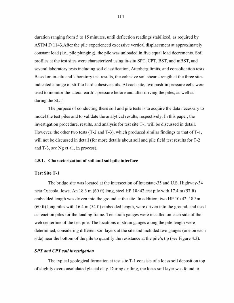
114

duration ranging from 5 to 15 minutes, until deflection readings stabilized, as required by

ASTM D 1143.After the pile experienced excessive vertical displacement at approximately

constant load (i.e., pile plunging), the pile was unloaded in five equal load decrements. Soil

profiles at the test sites were characterized using in-situ SPT, CPT, BST, and mBST, and

several laboratory tests including soil classification, Atterberg limits, and consolidation tests.

Based on in-situ and laboratory test results, the cohesive soil shear strength at the three sites

indicated a range of stiff to hard cohesive soils. At each site, two push-in pressure cells were

used to monitor the lateral earth‘s pressure before and after driving the piles, as well as

during the SLT.

The purpose of conducting these soil and pile tests is to acquire the data necessary to

model the test piles and to validate the analytical results, respectively. In this paper, the

investigation procedure, results, and analysis for test site T-1 will be discussed in detail.

However, the other two tests (T-2 and T-3), which produced similar findings to that of T-1,

will not be discussed in detail (for more details about soil and pile field test results for T-2

and T-3, see Ng et al., in process).

4.5.1. Characterization of soil and soil-pile interface

Test Site T-1

The bridge site was located at the intersection of Interstate-35 and U.S. Highway-34

near Osceola, Iowa. An 18.3 m (60 ft) long, steel HP 10×42 test pile with 17.4 m (57 ft)

embedded length was driven into the ground at the site. In addition, two HP 10x42, 18.3m

(60 ft) long piles with 16.4 m (54 ft) embedded length, were driven into the ground, and used

as reaction piles for the loading frame. Ten strain gauges were installed on each side of the

web centerline of the test pile. The locations of strain gauges along the pile length were

determined, considering different soil layers at the site and included two gauges (one on each

side) near the bottom of the pile to quantify the resistance at the pile‘s tip (see Figure 4.3).

SPT and CPT soil investigation

The typical geological formation at test site T-1 consists of a loess soil deposit on top

of slightly overconsolidated glacial clay. During drilling, the loess soil layer was found to

115

extend to 9.25 m (30.3 ft) below the ground‘s surface. Using laboratory tests conducted on

disturbed samples collected during drilling, the two soil layers (loess and glacial clay) were

classified as low plasticity clay (CL) per the Unified Soil Classification System. The

groundwater table at the time of in-situ testing was located at 10 m (32.8 ft) below the

ground‘s surface. In addition to basic soil properties, Figure 4.3 summarizes the measured

CPT tip resistance (qc) and skin friction (fs), as well as the soil‘s undrained shear strength

(Su) estimated according to the CPT commonly used correlation recommended by

Schmertmann et al. (1978), using Nk = 15. Also included in this figure are the SPT blow

counts corrected to account for the effect of the soil overburden pressure, the locations of the

BST and mBST tests, and the effective shear strength parameters obtained from the BST

tests (discussed in detail in a subsequent section). Table 4.1 provides a summary of the soil

classification and the cone parameters from CPT results after considering the effect of the

pore water pressures.

Monitoring lateral earth pressure

At each site, conventional and modified BSTs at different normal stresses were

conducted at different depths to measure soil shear strength parameters and adequately

capture t-z curves for the soil-pile interface for main soil layers. To determine normal stresses

used in the BSTs and mBSTs conducted at each depth, the expected range of lateral earth

pressures on the surface of the pile along its length was required. For each test site, several 1-

D consolidation tests were conducted to cover the main soil layers along the pile‘s embedded

length. From laboratory consolidation tests, the coefficient of consolidation (Cv) and the

overconsolidation ratio (OCR) were calculated and summarized in Table 4.1 for the three test

sites. From the OCR values, the soil was mainly found to be from normally to slightly over

consolidate for the three test sites. Consequently, the at-rest lateral earth pressure coefficient

(Ko) was then determined using the equations recommended by Jaky (1944) for clays. The

values of Ko for NC soils and slightly OC soils ranged from 0.44 to 0.47 for all soil layers

along the length of the pile at T-1.

In addition to all in-situ tests used to estimate the lateral earth pressures, two push-in

pressure cells, which measure total lateral earth pressure and pore water pressure, were

116

installed near the test piles to: (1) validate the estimated lateral earth pressure calculated from

different in-situ tests, (2) ensure the applied normal stresses during the mBST represented the

lateral earth pressure on the pile, and (3) examine the effect of pile driving, if any, on the

lateral earth‘s pressure. The pressure cells were installed approximately two days before the

start of pile driving to allow for pressure readings to stabilize as recommended by Suleiman

et al. (2010) and data were continuously recorded as a function of time during pile driving,

restrikes, and SLT.

At test site T-1, the two push-in pressure cells were installed at distances of 20 cm

(8.0 inch) and 45.72 cm (18 inch) from the test pile flange, both at the same depth of 7.0 m

(23.25 ft) from the ground‘s surface. At the time of the SLT, the effective lateral earth

pressure, using the pressure cell closer to the pile, matches the estimated lateral earth‘s

pressure from SPT and CPT data, while the effective lateral earth‘s pressure, using the far

pressure cell, was higher than the range of the expected pressures. However, it was observed

the far pressure cell was broken when retrieved after testing, indicating damage that could

have occurred during installation. Consequently, the lateral earth pressure readings obtained

from the second pressure cell were disregarded and the average of measured and calculated

lateral earth pressures were used in this study.

BST and mBST soil investigation

The conventional and modified BSTs were conducted at depths of 2.7 m (8.8 ft), 7.2

m (23.6 ft), and 11.0 m (36.1 ft) below the ground‘s surface. The locations of conventional

and modified BST tests were selected to cover the main soil layers at the site. Based on the

lateral earth‘s pressure calculations and measurements presented above, the values of the

normal stresses along the test pile were determined, and the BST and mBST were conducted

accordingly. The Mohr-Coulomb failure envelope for the soil and the soil-pile interface

obtained from the BST and mBST results, respectively, are indicated as shown in Figure 4.4

at a depth equal to 11.0 m (36.1 ft) below the ground‘s surface. As expected, the figure

shows smaller values for adhesion (a) and friction angle (α) at the soil-pile interface, when

compared to the soil‘s shear strength parameters. Table 4.2 summarizes the measured soil‘s

shear strength parameters (i.e., c' and ϕ') and soil-pile interface properties (i.e., adhesion, a,

and friction angle, α), using BST and mBST, respectively. The table also summarizes the

117

selected values of normal stresses conducted with each test.

For test site T-1, the measured t-z curves obtained using the mBST at the soil-pile

interface are presented in Figure 4.5 for different depths along the pile embedded length,

using the corresponding appropriate normal stresses indicated in Table 4.2. Other t-z curves

measured, using the mBST based on different normal pressures and for other test sites, are

available but not presented in this paper due to size limitations; for more details see Ng et al.

(in process). In the ―t-z Analysis‖ section of this paper, the t-z curves measured, using the

mBST, are compared with those developed, based on the CPT test and the curves back-

calculated from strain gauge readings obtained during the SLT.

Test Sites T-2 and T-3

The typical geological formation at test sites T-2 and T-3 consists of loess soil deposit

on top of slightly overconsolidated glacial clay. Similar to T-1, the soil profiles at test sites T-

2 and T-3 were characterized using in-situ SPT, CPT, BST, and mBST, and laboratory tests

such as soil classification, Atterberg limits, and consolidation tests. Furthermore, two push-in

pressure cells were used to monitor the lateral earth‘s pressure. Soil classification and CPT

results at both sites are summarized in Table 4.1, which show a predominant cohesive soil

profile at both sites with the soil profile mainly consisting of clay and silty clay for T-2 and

clay to sandy silt for T-3. Table 4.1 shows CPT tip resistance (qc) at the three sites ranges

from 1249 kPa (26 ksf) to 9731 kPa (203 ksf) with estimated undrained shear strength from

79 kPa (1.7 ksf) to 288 kPa (6 ksf), indicating stiff to hard cohesive soils.

In-situ BST sand mBSTs were conducted, following the same procedures used forT-1

at different normal stresses as summarized in Table 4.2. In summary, a total of 16 and 18

conventional and/or modified BSTs were conducted at T-2 and T-3, respectively. Field

testing results showed similar trends to those found at T-1 and the t-z curves for both test

sites were developed using the same approach described previously. For the three sites, the

effective cohesion ranges from 13.3 kPa (278 psf) to 72.6 kPa (1517 psf).

4.5.2. Pile static load tests

For test site T-1, the load-displacement response measured at the pile‘s head is

118

presented in Figure 4.6, while the load distribution along the pile, established using the strain

gauge data recorded at the end of each load increment is shown in Figure 4.7. Figure 4.6

indicates the vertical load-displacement of the pile was approximately linear up to an applied

load of 1043 kN (236 kips), with the maximum applied load reached during testing, 1170 kN

(263 kips). The rate of load transfer in the pile during the last few loading steps, indicated by

the slope of the curves in Figure 4.7, was almost constant in both soil layers with the slope

for the top soil layer smaller than that of the bottom soil layer (i.e., 30 kN/m (2.1 kip/ft) vs.

90 kN/m (6.2 kip/ft)). Furthermore, the load transferred to the pile‘s tip during the test ranged

from 0 to 54 kN (0 to 12 kips), within 6% of the maximum applied load, confirming the

tested pile was essentially a friction pile.

The load-displacement along the pile shaft was determined by integrating strain

gauge data using Simpson‘s numerical integration rule. The pile tip load-displacement curve

was then back-calculated by subtracting the total load-displacement measured at the pile‘s

head from the integrated load-displacement along the pile‘s shaft. The total load-

displacement response measured at the pile‘s head, as well as separated shaft and tip

displacements are presented in Figure 4.6, showing the pile capacity was approximately 1100

kN (243 kips), based on Davisson‘s criterion (Davisson, 1972).

Similar to T-1, an instrumented steel HP 10x42 test pile, with a length of 18.3 m (60

ft), was driven into the ground after conducting the BSTs at T-2 and T-3 test sites. For T-2

and T-3, the rate of load transfer during the last few loading steps for the loess and glacial

clay soil layers was comparable to that measured at T-1. Using Davisson‘s criterion, the pile

capacity at T-2 and T-3 was 685 kN (154 kips) and 700 kN (157 kips), respectively. Using

the strain gauge measurement, the maximum percent of load resisted by the pile‘s tip was 2%

for T-2 and 17% for T-3, confirming that the test piles mainly resisted the applied loads by

skin friction. Detailed soil properties, test results, and developed t-z curves for T-2 and T-3

can be found in Ng et al. (in process).

4.6. T-z Analysis

In each t-z model developed for the field tested piles, the HP 10x42 pile was divided

into 50 segments with each segment represented by an elastic spring of constant stiffness

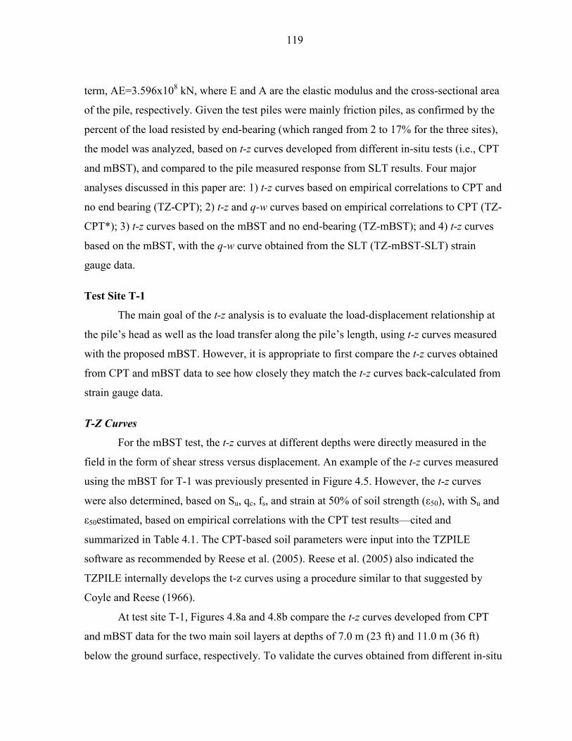
119

term, AE=3.596x108 kN, where E and A are the elastic modulus and the cross-sectional area

of the pile, respectively. Given the test piles were mainly friction piles, as confirmed by the

percent of the load resisted by end-bearing (which ranged from 2 to 17% for the three sites),

the model was analyzed, based on t-z curves developed from different in-situ tests (i.e., CPT

and mBST), and compared to the pile measured response from SLT results. Four major

analyses discussed in this paper are: 1) t-z curves based on empirical correlations to CPT and

no end bearing (TZ-CPT); 2) t-z and q-w curves based on empirical correlations to CPT (TZ-

CPT*); 3) t-z curves based on the mBST and no end-bearing (TZ-mBST); and 4) t-z curves

based on the mBST, with the q-w curve obtained from the SLT (TZ-mBST-SLT) strain

gauge data.

Test Site T-1

The main goal of the t-z analysis is to evaluate the load-displacement relationship at

the pile‘s head as well as the load transfer along the pile‘s length, using t-z curves measured

with the proposed mBST. However, it is appropriate to first compare the t-z curves obtained

from CPT and mBST data to see how closely they match the t-z curves back-calculated from

strain gauge data.

T-Z Curves

For the mBST test, the t-z curves at different depths were directly measured in the

field in the form of shear stress versus displacement. An example of the t-z curves measured

using the mBST for T-1 was previously presented in Figure 4.5. However, the t-z curves

were also determined, based on Su, qc, fs, and strain at 50% of soil strength (ε50), with Su and

ε50estimated, based on empirical correlations with the CPT test results—cited and

summarized in Table 4.1. The CPT-based soil parameters were input into the TZPILE

software as recommended by Reese et al. (2005). Reese et al. (2005) also indicated the

TZPILE internally develops the t-z curves using a procedure similar to that suggested by

Coyle and Reese (1966).

At test site T-1, Figures 4.8a and 4.8b compare the t-z curves developed from CPT

and mBST data for the two main soil layers at depths of 7.0 m (23 ft) and 11.0 m (36 ft)

below the ground surface, respectively. To validate the curves obtained from different in-situ

120

tests, the t-z curves at the same depths were back-calculated using the strain gauge data.

When compared to the t-z curves from mBST and CPT data, Figure 4.8 shows that the t-z

curves measured, using mBST, provide a reasonable match with the curves back-calculated

from the strain gauge data. The t-z curves obtained, using CPT, did not match the back-

calculated curves, especially for the soil‘s layer at 11.0 m (36 ft). This confirms the mBST

data better represents the soil-pile interface properties when compared with the CPT data and

it can be used to directly measure the t-z curves required for the load-transfer analysis.

Analysis and results

The calculated load-displacement relationships using the t-z curves developed from

CPT and mBST data compared with the measured SLT response for the friction steel H-pile

at test site T-1 are summarized in Figure 4.9. The key values of the calculated responses are

compared with the measured responses and have been summarized in Table 4.3. For test site

T-1, the slope of the first portion of the load-displacement curve (i.e., the load-displacement

curve before the start of plunging failure) calculated from the TZ-CPT model provided a 37%

stiffer response when compared with the slope of the first portion of the measured curve from

the SLT. The pile capacity estimated using Davisson‘s criterion for the TZ-CPT analysis was

1654 kN (372 kips), 50% higher than the measured pile capacity of 1100 kN (247 kips). This

significant overestimation of the CPT-based approach is consistent with observations for T-2

and T-3. When including the effect of the end bearing component using a q-w curve

developed based on CPT data, the results of the TZ-CPT* analysis showed an insignificant

difference of 3% compared to the TZ-CPT model, where end-bearing was ignored.

Therefore, considering the q-w curve, based on CPT data, did not significantly affect the

calculated response.

The analysis using the t-z curves directly measured in the field, using mBST (TZ-

mBST) did not include the q-w curve for end-bearing. They show a slope of the first portion

of the load-displacement response approximately 3% softer than the measured response (see

Figure 4.9). Furthermore, the pile capacity estimated using Davisson‘s criterion from the TZ-

mBST analysis was 25% smaller than the pile capacity estimated from the measured

response (see Table 4.3). However, when the TZ-mBST predicted capacity was compared

with the measured capacity based on skin friction only, the difference is reduced from 25 to

121

19%. Therefore, the TZ-mBST has provided a conservative, yet acceptable, prediction of pile

capacity, when compared to the significantly overestimated capacity provided by the TZ-

CPT model. Generally, it is clear the TZ-mBST analysis has improved the prediction of pile

behavior and provided a better load-displacement response compared to that calculated,

based on empirical correlations using CPT data.

Although not practical for prediction purposes, an additional analysis similar to TZ-

mBST was conducted, where the end-bearing component back-calculated from strain gauge

data was included. In this analysis, referred to as TZ-mBST-SLT, it was found that

incorporating the end-bearing component slightly improves the prediction of the slope of the

first portion of the load-displacement curve, reducing the difference between the measured

and calculated responses from 3 to 1% (see Figure 4.9 and Table 4.3). Pile capacity obtained

from the TZ-mBST-SLT model was 980 kN (220 kips), only 11% smaller than the measured

capacity.

In conclusion, although the t-z analysis, based on mBST data, was slightly

conservative when estimating pile capacity, it provided a very good match of the slope of the

first portion of the load-displacement curve (i.e., the load-displacement curve before the start

of plunging). Ignoring the end-bearing component in the TZ-mBST model could have caused

this conservatism, which was reduced in the TZ-mBST-SLT model. However, the TZ-mBST

as well as the TZ-mBST-SLT models better represent the pile measured load-displacement

relationship compared to the TZ-CPT model. This improved prediction of the first portion of

the load-displacement curve, which represents the range of working stresses for these piles,

could be used to incorporate serviceability limits into the LRFD approach for deep

foundation design.

In addition to comparing the load-displacement responses, the load distribution along

the length of the pile calculated, using different t-z models was compared with the measured

load distributions obtained from strain gauge data. Figure 4.10 represents the load

distribution along the pile‘s length at an applied load of 880 kN (198 kips), using different t-z

analyses compared to the measured distribution. This figure shows the TZ-mBST and TZ-

mBST-SLT models provide a very good prediction of the load distribution along the pile‘s

length compared to the TZ-CPT model. It should be noted the inaccurate load-displacement

122

relationship and load distribution prediction of the CPT-based approach may be improved by

conducting extensive field and laboratory tests to determine the most appropriate empirical

correlation to use for a specific site and pile condition. However, using the proposed mBST-

based approach avoids this problem.

Test Sites T-2 and T-3

Figures 4.11 and 4.12 show the load-displacement curves for the piles at test sites T-2

and T-3, respectively, using the same four t-z models discussed above, and compared with

the measured responses from the SLT results. Figure 4.11 shows similar responses to those

presented in Figure 4.9 at test site T-1. Table 4.3 also summarizes the characteristics of the

calculated load-displacement curves at test sites T-2 and T-3 compared with the measured

responses obtained from SLTs. The load-displacement curve resulting from the TZ-CPT

model provided a significantly higher slope of the first portion of the load-displacement

curve compared to SLT results and a significantly higher pile capacity, based on Davisson‘s

criterion (see Table 4.3). On the other hand, the analysis using the TZ-mBST model provided

a very good match to the first portion of the measured load-displacement curve as well as

closer Davisson pile capacities when compared to the TZ-CPT results. Moreover, Figures

4.11 and 4.12 represent the results of the TZ-mBST-SLT model. They are clear, considering

the end-bearing component did not significantly affect the calculated load-displacement

relationship. In summary, a similar soil-pile response to that observed at T-1 was observed at

T-2 and T-3.

4.7. Summary and Conclusions

Although t-z analysis has proven a practical method for modeling vertically-loaded

deep foundations, the t-z and q-w curves are typically based on empirical or semi-empirical

correlations with soil properties measured or estimated using laboratory or in-situ soil tests.

To improve the load-transfer analysis used to predict the load-displacement and load transfer

along the pile‘s length, a modified Borehole Shear Test (mBST) is proposed to directly

measure the t-z curves in the field. For steel H-piles, the mBST uses smooth steel plates to

measure the shear stress as a function of displacement at the soil-pile interface at different

123

normal stresses. In this study, a load-transfer analysis was conducted, based on the measured

soil-pile interface properties using the mBST, and the empirically correlated interface

properties from CPT results.

Three full-scale instrumented load tests were conducted on driven friction steel HP

10x42 piles at three sites with mainly cohesive soil profiles. The measured responses of the

load tests included vertical load-displacement at the pile‘s head and load transfer along the

length of the pile. The soil‘s profiles at the three sites were characterized using SPT, CPT,

BST, and mBST tests. The t-z curves were developed using CPT and mBST for soil layers at

three different sites. The calculated responses, using the t-z models, were compared with the

measured responses. Four major t-z models were analyzed for each test pile: TZ-CPT, TZ-

CPT*, TZ-mBST, and TZ-mBST-SLT. The first and the third models ignored the end-

bearing component (since the test piles were mainly friction piles), while the second and the

fourth models consider end-bearing, based on CPT and SLT, respectively. When compared

with measured responses for the three sites, the major findings from this study can be

summarized as follows:

The pile load-displacement relationship predicted using t-z curves, based on empirical

correlations with CPT data (TZ-CPT), significantly overestimated the soil-pile

interface properties, the first portion of the load-displacement response, and the pile

capacity by as much as 50%.

The pile load-displacement response calculated using t-z curves obtained from mBST

data (TZ-mBST) provided a very good match of the slope of the first portion of the

measured load-displacement responses (i.e., the load-displacement curve before the

start of plunging) and an acceptable estimate of the pile‘s capacity (with differences

ranging from 17 to 25% for the three test sites).

Ignoring the end-bearing component (q-w curve) in the t-z analysis did not

significantly affect the results in the case of friction steel H-piles.

Based on overall response predictions for the three test sites, the TZ-mBST model has

proven to provide a better match of the measured SLT results when compared with

TZ-CPT model.

Finally, the proposed mBST is a simple, cost effective in-situ test that captures the

124

soil-pile interface properties and can be directly used in the load-transfer analysis to simulate

load-displacement behavior at the pile‘s head and the load distribution along the pile‘s

length. This study focused on friction steel H-piles in cohesive soils. However, it can be

extended to other types of deep foundations such as concrete piles. The proposed procedure

can also help incorporate serviceability limits into the LRFD for deep foundation design.



research project TR-573: Development of LRFD Design Procedures for Bridge Pile in Iowa,

funded by the Iowa Highway Research Board (IHRB). The authors express their gratitude to

the IHRB and members of the project Technical Advisory Committee for their guidance and

advice. The members of this committee represent Office of Bridges and Structures, Soils,

Design Section, and Office of Construction of the Iowa DOT, FHWA Iowa Division, and

Iowa County Engineers. Finally, special thanks to Kam Weng Ng and Matthew Roling for

their help during conducting the field/laboratory tests and interpretation of data.

4.9. References

AbdelSalam, S. S., Sritharan, S., and Suleiman, M. T. (2008). ―Current Design and

Construction Practices of Bridge Pile Foundations.‖ International Foundation

Congress and Equipment Expo 09, ASCE and Geo-Institute, Orlando, Florida.

Abu-Farsakh, M. Y. and Titi, H. H., (2004). ―Assessment of Direct CPT Methods for

Predicting the Ultimate Capacity of Friction Driven Piles.‖ ASCE Journal of

Geotechnical and Geoenvironmental Engineering, volume 130, No. 9, pp. 935 - 944.


Cohesionless soils under Tensile Loading.‖ Computers and Geotechnics 32, 578–586.

American Society for Testing of Materials (2007).―Standard Test Methods for Deep

Foundations under Static Axial Compressive Load.‖ ASTM D1143 – 07.

Coyle, H. M. and Reese, L. C. (1966). ―Load Transfer for Axially-loaded Piles in Clay.‖



125


De Gennaro, V., Said, I., and Frank, R. (2006).―Axisymmetric and 3D Analysis of Pile Test


Francis Group, London, ISBN 0-4 15-40822-

El-Mossallamy, Y. (1999). ―Load-Settlement Behavior of Large Diameter Bored Piles in

Over-consolidated Clay.‖ Proceeding: The 7th

International Symposium on Numerical

Models in Geotechnical Engineering - NUMOG VII, Graz, 1-3 September 1999, 433-

450. Rotterdam, Balkema.


Elements for the Modeling of Piles.‖ Proceeding: 10th

International Symposium on

Numerical Models in Geotechnical Eng. – NUMOG X, Rhodes (Greece). April 2007.

Guo, W. D. and Randolph M. F. (1998). ―Vertically Loaded Piles in Non-homogeneous

Media.‖ Inter. Jl. for Numerical and Analytical Methods in Geomechanics, Vol. 21.

Handy, R. L. (1986). ―Borehole Shear Test and Slope Stability.‖ Proceeding: The ASCE

Specialty Conference on In Situ tests: Use of In Situ Tests in Geotechnical

Engineering, Blacksburg, Virginia, pp. 161-175.

Handy, R. L. (2008). ―Evaluation of Geotechnical soil Testing I. Field Tests.‖International

Journal of Geotechnical Engineering, 1, pp. 11-28.

Handy, R. L. and Fox, N. S. (1967). ―A Soil Borehole Direct Shear Test Device.‖ Highway

Research News, Transportation Research Record, No.27, p. 42-51.

Jaky, J. (1944). ―The Coefficient of Earth Pressure at Rest.‖Journal of Society of Hungarian

Architects and Engineers, Budapest, Oct. 1944, pp. 355-358.

Mayne, P. W. and Kulhawy, F. H. (1990). ―Manual on Estimating Soil Properties for

Foundation Design.‖ Rpt. EL-6800, Electric Power Research Inst., Palo Alto, 306 p.

Misra, A. and Chen, C. H. (2004). ―Analytical Solutions for Micropile Design under Tension




Ng, K. W., Sritharan, S., Suleiman, M., AbdelSalam, S. S., & Roling, M. (in

process).―Development of LRFD Design Procedures for Bridge Pile Foundations in

126

Iowa - Soil Investigation and Full-Scale Pile Tests.‖ Final Report Vol. II. IHRB

Project No.TR-573, TR-583 and TR-584.Iowa State University, Ames, Iowa.

Reddy, E. S., O‘Reilly, M., and Chapman, D. A. (1998). ―Modified t-z Model- A Software

For Tension Piles.‖ Computers and Structures, 68: 613–25.

Reese, L. C., Wang, S. T., and Arrellage, J. (2005). ―Analysis of Load Versus Settlement for

an Axially-loaded Deep Foundation - TZPILE v.2.0 Software User Manual.‖

ENSOFT, INC.3003 West Howard Lane, Austin, Texas 78728.


Methodology for Service Limit State Design of Deep Foundations using a t-z Model


Robertson, P. K., and Campanella, R. G. (1983). ―Interpretation of Cone Penetration Tests.‖


Schmertmann, I. B. (1978). ―Guidelines for Cone Penetration Test, Performance, and

Design.‖ Report No. FHWA-TS-78-209, U.S. DOT, Washington, D.C., pp. 145.

Suleiman, I. B. and Coyle, H. B. (1976). ―Uplift Resistance of Piles in Sand.‖ Journal of


Suleiman, M. T., Conway, W. M. Stevens, L. Jahren, C. T., Ceylan, H. (2010).

―Identification of Practices, Design, Construction, and Repair Using Trenchless

Technology.‖ Institute of Transportation, Final Research Report. Iowa Department of

Transportation Project Number IHRB-06-09.


127

Table 4.1: Soil properties measured in laboratory and estimated using SPT and CPT

Test

# Layers

m

Soil

Type(1) γ(2)

kN/m3 qc

kPa

fs kPa

OCR (3)

Cv(3)

in2/min Ko

(4) Su

(5) kPa

ϕ (6) ε50

(7)

T-1 0 – 8.5 CL 17.5 1673 102 1.11 0.031 0.47 107 -- 0.0050

8.5 – 17.4 CL 22 2908 153 < 1.0 0.024 0.44 180 -- 0.0045

T-2

0 - 1.5 Fill 17 1543 64 1.0 0.042 0.42 101 -- 0.0050

1.5 - 5.5 CL-ML 18.2 1614 12 1.41 0.026 0.44 102 29 --

5.5 - 10.7 CL 18.9 2815 172 < 1.0 0.026 0.47 177 -- 0.0045

10.7 – 17 CL 19.5 2165 74 < 1.0 0.035 0.51 129 -- 0.0050

T-3

0 – 6.6 CL 17.5 1249 62 N/A N/A 0.48 79 -- 0.0070

6.6 -11.4 ML 19.0 9731 62 4.43 0.044 0.44 638 32 --

11.4 – 15 CL 21.0 3771 74 < 1.0 0.067 0.45 236 -- 0.0040

15 – 17.4 CL 22.0 4628 206 < 1.0 0.024 0.44 288 -- 0.0040

For unit conversion: 1 m = 39.37 inch; 1 kN/m3 = 6.24 lb/ft

3; and 1 kPa = 0.145 psi.

(1) CL is low plastic clay, CL-ML is silty clay, and ML is sandy silt (according to the USCS);

(2)Soil total unit

weight calculated in the laboratory; (3)

OCR and coefficient of consolidation (Cv) measured based on a

laboratory conducted 1-D consolidation tests; (4)

Ko calculated for normally consolidated clays after Jaky (1944)

based on CPT results; (5)

After Schmertmann et al. (1978), assuming Nk=15; (6)

After Robertson and

Campanella; and(7)

After Reese et al. (2005) used for the TZ-CPT analysis.

Table 4.2: Soil and soil-pile interface shear strength parameters measured using the BST and

mBST at different depths showing the range of normal stress

Test# Depth

(m) Range of Normal Stress

Pn (kPa)

BST(1) mBST

(2)

c' (kPa) ϕ' a (kPa) α

T-1

2.7 22 30* 40 60 14.9 25 15.1 22

7.2 50 70 90 110* 26.2 7 18.1 7

11.0 110 130 150 170* 72.6 27 42.2 15

T-2 8.2 60 80 100 120* 22.7 8 12.6 16

14.0 150 180 200 220* 13.6 12 14.4 10

T-3

2.7 20 40* 80 N/A 7.0 33 1.5 27

7.0 50 100 150* N/A 13.3 14 22.0 5

13.7 100 150 250* N/A 48.6 3 38.3 15 For unit conversion: 1 m = 39.37 inch; and 1 kPa = 0.145 psi. (1)

Conventional BST, using test procedures after Handy (1986) to allow for pore water pressure dissipation; (2)

Modified BST, using similar testing procedures to the conventional test to allow for pore water pressure

dissipation; and *Represents the normal stress corresponding to measured lateral earth pressure and

selected for the TZ-mBST analysis.

128

Table 4.3: Summary of the major t-z analyses used to compare the calculated responses with

the measured responses from SLT

Test

# Model

Model Description Load-Displacement

Curve % Difference to SLT

(1)

t-z

curves (skin-

friction)

q-w

curve (end-

bearing)

Slope of

First

Portion

(kN/m)

Davisson Capacity

(kN)

Slope of

First

Portion

Davisson Capacity

T-1

SLT Strain Gauges 193116 1100 Measured

TZ-CPT CPT Ignored 265054 1654 37% stiffer 50% higher

TZ-CPT* CPT CPT 265054 1680 37% stiffer 53% higher

TZ-mBST mBST Ignored 184257 830 3% softer 25% lower

TZ-mBST-SLT mBST SLT 190415 980 1% softer 11% lower

T-2




TZ-mBST mBST Ignored 195377 566 2% softer 17% lower

TZ-mBST-SLT mBST SLT 187526 570 6% softer 17% lower

T-3




TZ-mBST mBST Ignored 177972 840 5% stiffer 20%higher

TZ-mBST-SLT mBST SLT 176870 920 5% stiffer 31% higher (1)

Difference between the load-displacement curves adapted from different t-z analyses and the pile

measured response during SLT.

129

Figure 4.1: Idealized load-transfer model showing t-z curves for the pile segments and q-w

curve at the pile tip (modified after Alawneh, 2006)

Figure 4.2: (a) BST components (modified after Handy, 2008, courtesy of Handy

Geotechnical Instruments, Inc.); (b) added dial gauge; (c) grooved shear plates used in

conventional BST; (d) new smooth plates; and (e) sample t-z curve

She

ar S

tre

ss

q-w curve at pile tipt-z curves along the shaft

K

t

z

Dynamometer

Shear Head

She

ar S

tre

ss

Displacement

130

Figure 4.3: Summary of soil tests conducted at T-1 including: tip resistance (qc), skin

friction (fs), and undrained shear strength (Su) from CPT; corrected SPT N-values; depths

of BST/mBST, and soil shear strength parameters from BST; soil classification; and strain

gauges locations

0

10

20

30

40

50

60

0 1000 2000 3000 4000 5000 6000

0

2

4

6

8

10

12

14

16

18

20

0 50 100 150 200 250 300

De

pth

(ft)

qc (kPa)

De

pth

(m)

fs and Su (kPa)

fs

Su

qc

SG-1

SG-2

SG-3

SG-4

SG-5

SG-6

SG-7

SG-8

SG-9

SG-10

12

10

10

12

9

9

19

17

Strain Gauges

Location of Strain Gauges Location of SPT

Pile Head

Pile ToeSG: Strain Gauge

Corrected SPTN-values

Low Plasticity Clayγ = 17.5 kPaL.L. = 49%P.I. = 27%

c’ = 20.5 kPaφ’ = 16o

Low Plasticity Clayγsat = 22 kPaL.L. = 42.3%P.I. = 24.6%c’ = 72.6 kPaφ’ = 27o

Ground Surface

GWT

BST-1

BST-2

BST-3

131

Figure 4.4: Failure envelopes for the soil and soil-pile interface measured using BST and

mBST, respectively, at a depth of 11.0 m below the ground surface for T-1

Figure 4.5: Shear stress vs. displacement curves for the soil-pile interface measured using

mBST at different depths below ground surface and at the normal stresses used in the t-z

analysis for T-1

0 5 10 15 20 25 30

0

5

10

15

20

25

0

20

40

60

80

100

120

140

160

180

0 50 100 150 200

Normal Pressure (psi)

She

ar S

tre

ss (

psi

)

She

ar S

tre

ss (

kPa)

Normal Pressure (kPa)

Conventional BST

Modified BST

c = 72.6 kPa, ф = 27o

a = 42.2 kPa, α = 15o

0 0.05 0.1 0.15 0.2 0.25

0

2

4

6

8

10

12

14

0

10

20

30

40

50

60

70

80

90

100

0 1 2 3 4 5 6 7

Displacement (inch)

She

ar S

tre

ss (

psi

)

She

ar S

tre

ss (

kPa)

Displacement (mm)

d=2.7 m and Pn=30 kPad=7.2 m and Pn=110 kPad=11.0 m and Pn=170 kPa

(d) is depth below ground surface; and (Pn) is normal stress

132

Figure 4.6: Measured pile load-displacement response at the pile head during static load test

and calculated pile shaft and pile tip displacement for test site T-1


different applied loads for test site T-1

0 50 100 150 200 250

0

0.2

0.4

0.6

0.8

0

5

10

15

20

0 250 500 750 1000 1250

Load (kips)

Dis

pla

cem

en

t (i

nch

)

Dis

pla

cem

en

t (m

m)

Load (kN)

Total LoadShaft ResistanceEnd Bearing

0 50 100 150 200 250 300

0

10

20

30

40

50

60

0

5

10

15

20

0 250 500 750 1000 1250

Load (kips)

De

pth

(ft

)

De

pth

(m

)

Load (kN)

6119132039952665979692510511170

Load (kN)

GroundSurface

Low Plastic Clay

Low Plastic CLay

Points at 18.3m were extrapolated6% end-bearing component

133

Figure 4.8: t-z curves developed from mBST and CPT compared with t-z curves back-

calculated from strain gauge data within the two major soil layers at depths of 7.0 and 11.0

m for test site T-1

0 0.05 0.1 0.15 0.2 0.25

0

5

10

15

20

25

0

20

40

60

80

100

120

140

160

180

0.00 1.00 2.00 3.00 4.00 5.00 6.00 7.00

Displacement (inch)

Un

it S

he

ar S

tre

ss (

psi

)

Un

it S

he

ar S

tre

ss (

kPa)

Displacement (mm)

SG (7.6 m)

mBST (7.2 m)

CPT (6.9 m)

(a)

0 0.05 0.1 0.15 0.2 0.25

0

5

10

15

20

0

20

40

60

80

100

120

140

160

0.00 1.00 2.00 3.00 4.00 5.00 6.00 7.00

Displacement (inch)

Un

it S

he

ar S

tre

ss (

psi

)

Un

it S

he

ar S

tre

ss (

kPa)

Displacement (mm)

SG (10.8 m)

mBST (11 m)

CPT (10.8 m)

(b)

134


measured response for test site T-1

Figure 4.10: Load distribution along the pile length calculated using different t-z analyses

compared with measured values at test site T-1

0 50 100 150 200 250 300 350 400 450

0

0.1

0.2

0.3

0.4

0.5

0.6

0

2

4

6

8

10

12

14

16

0 250 500 750 1000 1250 1500 1750 2000

Load (kips)

Dis

pla

cem

en

t (i

nch

)

Dis

pla

cem

en

t (m

m)

Load (kN)

SLT

TZ-CPT

TZ-mBST

TZ-mBST-SLT

0 50 100 150 200 250

0

10

20

30

40

50

60

0

2

4

6

8

10

12

14

16

18

20

0 250 500 750 1000

Load (kips)

De

pth

(m

)

Load (kN)

SLT

TZ-CPT

TZ-mBST

TZ-mBST-SLT

De

pth

(ft

)

135





0 50 100 150 200 250

0

0.1

0.2

0.3

0.4

0.5

0

2

4

6

8

10

12

14

0 250 500 750 1000 1250

Load (kips)

Dis

pla

cem

en

t (m

m)

Load (kN)

SLT

TZ-CPT

TZ-mBST

TZ-mBST-SLT

Dis

pla

cem

en

t (i

nch

)

0 50 100 150 200 250

0

0.2

0.4

0.6

0.8

1

0

5

10

15

20

25

0 200 400 600 800 1000 1200

Load (kips)

Dis

pla

cem

en

t (i

nch

)

Dis

pla

cem

en

t (m

m)

Load (kN)

SLT

TZ-CPT

TZ-mBST

TZ-mBST-SLT

136

CHAPTER 5: IMPROVED T-Z ANALYSIS FOR VERTICALLY LOADED PILES IN

COHESIONLESS SOILS BASED ON LABORATORY TEST MEASUREMENTS

Sherif S. AbdelSalam1; Muhannad T. Suleiman, M. ASCE

2; Sri Sritharan, M. ASCE

3

A paper to be submitted to the Journal of Geotechnical and Geoenvironmental Eng., ASCE

5.1. Abstract

Load transfer analysis (or t-z analysis) has been used to predict load-displacement

response of axially-loaded piles. The t-z curves along pile length and q-w curve at pile tip are

routinely obtained, based on empirical correlations using soil field or laboratory tests. This

study focuses on the use of a modified Direct Shear Laboratory Test (mDST) to directly

measure the t-z and q-w curves for steel piles driven into cohesionless soils. As part of this

study, two full-scale instrumented steel H-piles driven into sandy soils were load tested and

soil layers at the two sites were characterized using in-situ and laboratory soil tests. Load

transfer analyses, with t-z and q-w curves directly measured using the mDST, were

conducted to predict the response of full-scale load tests utilizing the TZPILE v.2.0 program.

When compared to the measured load-displacement response and load distribution as a

function of depth from the static load tests, the t-z models, based on mDST measurements,

showed very good match with the measured responses. The proposed method presents a

simple and cost-effective procedure to predict the pile response to aid in incorporating

serviceability limits into the design of deep foundations.

CE Database keywords: Load-transfer; t-z analysis; t-z and q-w curves; Load-displacement;

Direct shear test; Pile foundation.


Engineering, Iowa State University, 355 Town Engineering, Ames, IA 50011-3232, E-mail:[email protected] 2 Assistant Professor, Dept. of Civil and Environmental Engineering, Lehigh University, STEPs

Building, Room 326, 1 West Packer Avenue, Bethlehem, PA, 18015. E-mail: [email protected] 3

Wilson Engineering Professor and Associate Chair, Dept. of Civil, Construction and Environmental

Engineering, Iowa State University, 376 Town Engineering, Ames, IA 50011-3232, E-mail: [email protected]




137

5.2. Introduction

In the United States, bridges and their foundations are now designed using the Load

and Resistance Factor Design (LRFD) approach. In support of this, significant efforts have

been directed towards the development of LRFD resistance factors for deep foundations. The

current American Association of State Highway and Transportation Officials (AASHTO)

specifications and several locally-developed design guidelines provide resistance factors to

calculate pile resistance at the strength limit state, while the serviceability requirements that

may be needed to prevent excessive pile settlements are typically checked after determining

pile resistance. Thus, the typical design approach may not be efficient and may lead to

several design iterations to satisfy the strength and serviceability requirements, especially

when the serviceability limit state governs the design (Misra and Roberts, 2006). Therefore, a

design methodology, based on predicting pile load-displacement response can incorporate

both strength and serviceability limits in the design process (Misra et al., 2007; Roberts et al.,

2008). However, the analytical approach for predicting the load-displacement response needs

to be simple, yet it should produce acceptable accuracy for practicing engineers and

designers to use. Due to its efficiency, simplicity, and potential in developing the

serviceability limits for the design of deep foundations using the LRFD approach, load-

transfer numerical analysis, using the t-z method, was selected as an iterative technique that

solves nonlinear differential equations using the finite difference approach (Misra and Chen,

2004; Alawneh, 2006; Roberts et al., 2008).

The major shortcoming of the t-z analysis has been that no laboratory test was used to

accurately measure the load-transfer curves, t-z and q-w curves, to describe the skin-friction

between the pile and surrounding soil, and end-bearing at the pile‘s tip, respectively.

Therefore, the t-z and q-w curves have been estimated, based on empirical correlations to in-

situ soil tests, such as the Standard Penetration Test (SPT) or Cone Penetration Test (CPT)

(see Coyle and Reese, 1966; Roberts et al., 2008). Recently, AbdelSalam et al. (2010)

developed a modified Borehole Shear Test (mBST) that directly measures the t-z curves in

the field for the interface between the steel pile and cohesive soil. Given these test piles were

mainly friction piles, AbdelSalam et al. (2010) focused on measuring the t-z curves required

for modeling shaft resistance of the pile. When compared to measured responses from three

138

full-scale vertical load tests conducted on steel H-piles installed in cohesive soils, the t-z

analysis using load-transfer curves and mBST, showed good agreement with measured load-

displacement response at the pile‘s head and load transfer along pile length. However,

conducting mBST in cohesionless soils is not easy, due to the tendency of borehole collapse

and/or the risk of losing the mBST shear head during testing. In addition, the mBST can only

capture the t-z curves required for calculating the skin-friction component of the pile

resistance, acceptable in the case of friction piles driven into mainly cohesive soil profiles,

but in the case of cohesionless soils, the end-bearing component cannot be neglected.

The main objective of this study is to utilize the t-z analysis method to accurately

predict the load-displacement response of vertically-loaded steel H-piles driven into

cohesionless soils. For this purpose, a modified Direct Shear Test (mDST) was developed to

measure the t-z curves for different soil layers in the laboratory. In addition, the box for the

Direct Shear Test (DST) apparatus was used in a laboratory Pile Tip Resistance (PTR) test to

measure the q-w curve for the end-bearing soil layer. The proposed mDST and PTR

laboratory tests offer a simple and cost-effective method to directly measure the t-z and q-w

curves, respectively. These measured curves can be used with commercial software, TZPILE

v.2.0, developed by ENSOFT, Inc. to predict pile response using the t-z method. To validate

the proposed approach, two vertical static load tests (SLTs) were conducted on full-scale

instrumented steel H-piles driven into cohesionless soils at two different sites in Iowa and the

predicted responses were compared with those field measured.

5.3. Background

The use of DST to measure the soil-pile interface friction angle for steel piles was

initially proposed by Reddy et al. (2000) to estimate shaft capacity of steel piles driven into

sandy soils. Later, Pando et al. (2002) performed a series of tests to measure the fiber

reinforced polymer composite pile-soil interface friction angle. Pando et al. (2002) also

conducted comparisons to the static shaft capacity, based on the Nordlund static method

(Nordlund, 1963) and concluded the static calculated capacity using the interface angle

measured, using DST, showed comparable values with the measured capacity. However,

none of the studies cited above used DST to measure the t-z curves required for the load-

139

transfer analysis, or used the measured curves to predict pile load-displacement response and

compared the analysis with field measured responses from pile static load test results.

For the end-bearing mechanism, numerous studies have investigated soil response

under the pile tip utilizing small-scale models or calibrated chambers; several have focused

on measuring the load-penetration response that represents the q-w curve at the pile‘s tip. For

example, Houlsby and Evans (1988) studied steel pile bearing capacity in layered silts and

sands, using a soil-pile laboratory model to determine the effect of different pile types on the

load-penetration response. Yasufuku and Hyde (1995) investigated the relationship between

the soil stress-strain properties at the pile‘s tip and the corresponding end-bearing capacity.

However, neither of the previous studies used the laboratory measured load-penetration curve

to conduct a load-transfer analysis or compared their results to measured responses from

large-scale SLTs. Furthermore, determining the minimum permissible size of a soil-pile

laboratory model with respect to the pile diameter or size (D) is not detailed in the

aforementioned studies and has no clear design standards.

Nevertheless, Bowles (1996) indicated that soil stresses and corresponding

displacements at a pile tip bearing on dense sand or sand-gravel deposits can be evaluated,

with reasonable accuracy, assuming a fictitious rigid footing placed on the bearing stratum.

To model a rigid footing in a test pit or a small soil box, the ASTM D 1194 standards

(ASTM, 2006) states that the soil box size should be at least four times the width of the

model footing. Given the depth of stresses influence below the pile tip ranges from 2D to 4D

in different soils and is approximately 1.5D in the case of coarse sand deposits (Houlsby and

Evans, 1988), the minimum required depth of the soil box should be at least 1.5D below the

model rigid footing, bearing on dense sand or sand-gravel deposits. The summary provided

above shows that for piles installed in dense sand or sand gravel deposits, a laboratory test

with model rigid footing placed in a soil box with a width greater than 4D and depth greater

than 1.5D can be used. However, when using small-scale rigid footings to represent pile tip

response in dense sand or sand gravel deposits, the measured q-w curves for the model

footing must be scaled or converted to represent the q-w of the large-scale pile as will be

discussed later.

140

5.4. Field Testing

As part of an ongoing research project aimed at establishing LRFD resistance factors

for the design of deep foundations in the state of Iowa by accounting for local soil conditions,

ten vertical SLTs were conducted on full-scale instrumented steel HP 10x42 piles. The last

two SLTs were conducted on piles driven into cohesionless soil profiles (mainly sand) at Des

Moines County (test site ISU-9) and Cedar County (test site ISU-10). For ISU-9, the bridge

site was located southeast of Huron close to the Mississippi River. As for ISU-10, the bridge

was located south of Tipton at the intersection of Interstate-80 and the Iowa River. For both

test sites, a 15.8 m (52 ft) long test pile with 14.9 m (49 ft) embedded length was driven

between two anchor piles, 18.3m (60 ft) long with 16.4 m (54 ft) embedded length each. The

test piles were loaded, using a 2000 kN (440 kips) hydraulic jack, and the applied load was

measured using a 1300 kN (290 kips) load cell. The ―Quick Test‖ procedure outlined in the

ASTM D 1143 (ASTM, 2006) was used to load test the piles. In all cases, the load was

applied in 5% increments of the estimated nominal capacity and the load was kept relatively

constant at the end of each load increment for a duration ranging from 5 to 10 minutes until

the pile vertical displacement readings stabilized. After excessive vertical displacement at

approximately constant load was experienced, the piles were unloaded in five equal load

decrements. In addition to using four 25.4 cm (10 inch) displacement transducers to measure

the vertical displacement at the top of the two test piles, they were instrumented with strain

gauges along the shaft and near the tip.

Figures 5.1 and 5.2 show the locations of strain gauges installed on each side of the

web centerline of test piles ISU-9 and ISU-10, respectively. The locations of strain gauges

presented in the figures were determined, considering different soil layers at the two test sites

and included at least two gauges near the bottom of the piles to quantify tip resistance. The

soil profiles at the test sites were characterized, using in-situ SPT and CPT tests in addition to

several laboratory tests, including soil classification, Atterberg limits, as well as DST and

mDST. At ISU-10, a push-in pressure cell was used to monitor the lateral earth pressure

before and after driving of the piles as well as during SLT.

141

5.4.1. Soil investigation

SPT and CPT results

The typical geological formation at ISU-9 consists of normally consolidated

Alluvium deposits of clay, sand, and gravel deposits. As shown in Figure 5.1, four different

soil layers were found during drilling. The first layer consisted of clay deposits extending to

4.8 m (15.7 ft) below the ground surface, followed by sand deposits up to 13.4 m (43.9

ft),underlain by a 2.6 m (8.5 ft) of granular material, and the bottom layer consisted of firm

silty clay material. The groundwater table at the time of in-situ testing was located at 5.2 m

(17.1 ft) below the ground‘s surface. Using laboratory tests conducted on soil samples

collected at ISU-9, the top soil layer was classified as low plasticity clay (CL) per the Unified

Soil Classification (USCS), the second layer was classified as well-graded sand (SW), the

third as well-graded gravelly sand (SW), and the bottom layer as inorganic clay of high

plasticity clay (CH). In addition to the basic soil properties, Figure 5.1 summarizes the

measured CPT tip resistance (qc) and skin friction (fs) for ISU-9. Also included in Figure 5.1

are the SPT blow counts corrected for the effect of the soil‘s overburden pressure and the

corresponding relative density (Dr %) after Terzaghi and Peck (1967).

The soil profile at ISU-10 was divided into three layers, where the first layer

consisted of sandy fill material extending to 4.6 m (15.1 ft) below the ground surface

followed by a 10.4 m (34.1 ft) layer of coarse sand with gravel as presented in Figure 5.2.

The bottom layer consisted of sand and boulders, and the groundwater table was located 3 m

(9.8 ft) below the ground surface at the time of in-situ testing. Using laboratory tests

conducted on the soil samples from ISU-10, the top soil layer was classified as well-graded

sand (SW) per the USCS, the second layer was classified as well-graded sand with gravel

seam (SW), and the bottom layer as well-graded gravelly sand (SW). As shown in Figure 5.2,

a 1.0 m (3 ft) layer of boulders was located almost in the middle of the second layer, which

prevented the CPT from penetrating to the desired depth. Figure 5.2 summarizes the basic

soil properties, the measured qc and fs from the CPT results, the corrected SPT blow counts,

and the relative density (Dr %) of different soil layers at ISU-10.

142

5.4.2. Monitoring lateral earth pressure

In preparation for conducting conventional and modified laboratory DSTs at different

normal stresses to measure soil shear strength parameters and adequately capture the t-z and

q-w curves along the soil-pile interface, expected ranges of lateral earth pressure (ζh) acting

along the test piles were required to determine the appropriate normal stresses for use in the

DST and mDST tests. Figures 5.1 and 5.2 represent the location of DST/mDST for different

soil layers at ISU-9 and ISU-10. To complete this task, the angle of soil internal friction (ϕ)

and the over consolidation ratio (OCR) of soil layers were estimated, based on empirical

correlations with SPT and CPT in-situ tests. Based on SPT results, the ϕ and the OCR were

estimated after Peck, Hanson, and Thornburn (1974) and Mayne and Kemper (1988),

respectively. For CPT-based estimates, recommendations by Robertson and Campanella

(1983) and Mayne and Kulhawy (1990) were used. The at-rest lateral earth pressure

coefficient (Ko) was then determined by using the equations recommended by Jaky (1944)

and Mayne and Kulhawy (1990) for Normally Consolidated (NC) and Over Consolidated

(OC) soils, respectively. Figures 5.1 and 5.2 summarize the Ko, OCR, and the corresponding

effective ζv along the pile length for NC and OC soils for ISU-9 and ISU-10.

To validate the estimated lateral earth pressure calculated based on SPT and CPT

tests, a push-in pressure cell was installed at ISU-10 at 20 cm (8.0 inch) from the test pile

flange and 3.1 m (10 ft) below the ground surface. The pressure cell data were continuously

recorded during pile driving, re-striking, and SLT. On average, the effective lateral earth

pressure measured by the pressure cell at the time of SLT was 22 kPa (3.2 psi), very close to

the calculated value for NC soils at the same depth, using the theoretical correlations with

SPT and CPT results (see Figure 5.2).

5.4.3. Pile static load tests

For test pile ISU-9, the load distribution along the pile length was established and

presented in Figure 5.3, using the strain gauge data recorded at the end of each load

increment during SLT. Figure 5.3 shows the rate of load transferred in the pile during the last

nine load steps represented by the slope of the curves was almost zero within the top soil

layer, indicating the cohesive material did not significantly contribute to pile resistance.

143

Within the second and third soil layers, an average rate of load transfer of 30 and 75 kN/m

(2.1 and 5.1 kips/ft) was observed, respectively. Furthermore, the load transferred to the

pile‘s tip during the test ranged from 0 to 210 kN (0 to 47.2 kips), indicating an end-bearing

of approximately 28% of the maximum applied load.

The measured total load-displacement response of the ISU-9 pile is presented in

Figure 5.4. Accordingly, pile response was approximately linear up to 521 kN (117.1 kips)

and sustained a maximum applied load of 754 kN (169.5 kips). Based on Davisson‘s criterion

(Davisson, 1972), the pile nominal capacity was determined 704 kN (158.3 kips). The shaft

load-displacement was determined by integrating strain gauge data, using Simpson‘s

numerical integration rule (Figure 5.3). The load-displacement curve at the pile tip was then

back-calculated by subtracting the skin friction component from the total response measured

at the pile‘s head. A similar procedure was used for the test pile at ISU-10, although the

strain gauges were not functioning properly. This precluded an accurate separation of the

skin friction and the end-bearing components from the pile‘s total capacity. Figure 5.4

represents the load-displacement response measured at the pile‘s head for ISU-10, indicating

an approximate total nominal capacity of 580 kN (130.4 kips), based on Davisson‘s criterion.

5.5. Direct Measurement of Load-Transfer Curves

5.5.1. Modified direct shear test to measure the t-z curves

Conventional DST was modified to directly measure the t-z curves at the soil-pile

interface for steel H-piles at ISU-9 and ISU-10. A square steel plate, with the same grade of

the steel piles, was fabricated to fit into the lower half of the DST mold with dimensions

equal to 100 mm (3.94 inch) in width and 40 mm (1.57 inch) in height. As shown in Figure

5.5, the steel plate is placed in the lower half of the shear box, while the upper half is filled

with soil material compacted to match the soil unit weight and estimated relative density

summarized in Table 5.1. Soil samples collected below the ground water table were

submerged in de-aired water during testing. A normal stress equal to the estimated horizontal

stresses on the surface of the pile at the depth of the tested sample was applied. The mDST

was conducted following the ASTM D3080-98 (ASTM, 2006). While performing the mDST,

the shear stress versus horizontal displacement was recorded after correction of the reduced

144

shear contact area, which represents the interface properties between the soil and the steel

plate, or the t-z curve at the soil-pile interface.

For the test pile at ISU-9, conventional and modified DSTs were conducted on soil

samples collected at depths of 2.6 m (8.5 ft), 7.0 m (23 ft), and 13.7 m (45 ft) below the

ground‘s surface, covering the main soil layers at the test site. As an example of the

measured properties, Figure 5.6 shows the Mohr-Coulomb failure envelope for the soil and

the soil-pile interface obtained from DST and mDST results, respectively, at 7.0 m (23 ft)

below the ground surface at ISU-9. As expected, the figure shows smaller values for

adhesion (a) and friction angle (α) at the soil-pile interface, when compared to soil shear

strength parameters. For all soil layers at ISU-9, Table 5.1 summarizes the values of the

water content, dry and total soil unit weights, relative density, and normal stresses used

during laboratory testing, in addition to the measured soil shear strength parameters (i.e., c'

and ϕ'), and soil-pile interface properties (i.e., adhesion, a, and friction angle, α), using the

DST and the mDST, respectively.

Figure 5.7 presents the measured t-z curves obtained using mDST at the soil-pile

interface compared to those back-calculated from the strain gauge readings obtained from the

SLT data at ISU-9. As can be observed from the figure, there is a good match between the

laboratory and field measured t-z curves, especially when comparing the maximum shear

stress values of the top and bottom soil layers, as the difference did not exceed 5%. The t-z

curves presented in Figure 5.7 were measured at normal stresses corresponding to the

measured and/or estimated lateral earth pressure in the field (see Table 5.1). For test site ISU-

10, DST and mDST tests were conducted following the same procedures used for ISU-9 at

different normal stresses as summarized in Table 5.1. The table also summarizes the soil

shear strength parameters and soil-pile interface properties measured for the test pile at ISU-

10. The test results for ISU-10 showed similar trends to those observed for ISU-9.

Using the load transfer analysis, the t-z curves were measured by utilizing mDST to

predict pile load-displacement response. However, to include the end-bearing component, the

q-w curve at the pile tip is needed. In the following section, another modification is proposed

to the DST apparatus to measure the q-w curve at the pile‘s tip.

145

5.5.2. Pile tip resistance test to measure the q-w curves

As previously discussed, the response of the tip of a pile installed in sand deposits can

be modeled as rigid footing in the laboratory. A small-scale steel plate (representing a

fictitious rigid footing) was used to model the vertical load-displacement relationship (q-w

curve) under the pile‘s tip for ISU-9 and ISU-10. The box with the DST apparatus,

dimensions of 100 mm (3.94 inch) in width and 60 mm (2.36 inch) in height (see Figure 5.8),

was used in a laboratory Pile Tip Resistance (PTR) test to measure the q-w curve for a small-

scale steel plate.

To confirm the suggested relative dimensions between the soil box and the model

plate summarized in the background section, steel plates with different sizes and shapes were

tested. The box width to plate width ratios of 4 and 5.7 and box depth to plate width ratios of

2.4 and 3.4 were used. These plates were embedded by 10 mm (0.40 inch) in the compacted

soil. For the model representing ISU-9, the soil sample collected at a depth of 15 m (49.2 ft)

(i.e., the depth of the pile tip) was compacted inside the box to match the estimated Dr of

68%. For ISU-10, the sample collected at the pile‘s tip was compacted to achieve a Dr% of

76%. For both PTR tests at ISU-9 and ISU-10, the loads were applied in controlled steps

equal to one-twentieth of the estimated maximum load, following testing procedures

provided by Yasufuku and Hyde (1995). For each loading increment, the corresponding

vertical displacement was measured until the rate of settlement was less than 0.01 mm/min.

When comparing the measured responses of different plates, the difference in the

load-displacement curves measured using both steel plate sizes was determined less than

10%. Furthermore, the effect of placing the plate on the soil‘s surface was evaluated and

found its effect is also less than 10%. Therefore, using different sizes and placement

locations of steel plates did not significantly affect PTR test results. Hence, the box‘s

dimensions relative to the used steel plates were considered acceptable.

In addition to the previous laboratory checks on box dimensions, a finite element (FE)

analysis representing the used box in the PTR test, the soil, and the steel plate (with a box to

plate width ratio of 4.0) was conducted to confirm the dimensions of the box and the plate

have minimal effects on the measured responses. An axisymmetric FE model was used to

simulate the behavior, based on the Mohr-Coulomb constitutive model for the soil material,

146

using the commercial computer program, PLAXIS 7.2. In the axisymmetric analysis, the

model plate diameter of 28 mm (1.12 inch) was selected to provide the same cross-sectional

area of the actual steel plate. The plate was modeled as a non-porous linear-elastic material

with elastic modulus equal to 2x108 kPa (2.9x10

7psi) and Poisson‘s ratio equal to 0.2. The

soil‘s shear strength measurements from the DST laboratory test results (see Table 5.1) were

used for the required parameters of the Mohr-Coulomb soil constitutive model. The FE

model was manually adjusted to match the stress-displacement behavior measured from the

laboratory model. Presented in Figure 5.9 is the evaluated normal stress corresponding to the

prescribed vertical displacement of 7.0 mm (0.28 inch) for ISU-9. As seen from the figure,

the maximum stresses induced in the soil were concentrated directly below the steel plate and

degraded towards the bottom horizontal boundary to less than 18% of the maximum stress.

Moreover, the maximum vertical displacement under the plate did not exceed 1.4D, where D

is the diameter of the steel plate, even less than the minimum required depth of the soil box

specified in the literature. Thus, based on experimental results and finite element analysis, the

dimensions of the used box in the PTR test are large, compared to plate dimensions, and

insignificantly affect the vertical load-displacement response of the load tested plates.

The load-displacement response of the PTR model plate with box to plate width ratio

of 4.0 was used in the t-z analyses for ISU-9 and ISU-10. The measured load-displacement

curves for the model plate were converted to load-penetration curves (q-w curves) for the

full-scale pile at ISU-9 and ISU-10. According to Bowles (1988), the following expression

can be practically used to extrapolate the model plate loads in the case of cohesionless soils.

𝑞𝑝𝑖𝑙𝑒 = 𝑞𝑚𝑜𝑑𝑒𝑙 𝐴𝑝𝑖𝑙𝑒

𝐴𝑚𝑜𝑑𝑒𝑙

The qpile and qmodel represent the applied load on the full-scale pile and the model

plate, respectively. Apile and Amodel represent the full-size and the model pile cross-sectional

areas, respectively. By using the cross-sectional area ratio in the previous equation, the

square shaped PTR model pile can be practically converted for the full-size actual pile (H-

shaped). For displacement (w) calculations, Terzaghi and Peck (1967) provided an equation

to convert the measured tip displacement of the model pile to that of the full size pile in

147

cohesionless soils as follows:

𝑤𝑝𝑖𝑙𝑒 = 𝑤𝑚𝑜𝑑𝑒𝑙 2𝐴𝑝𝑖𝑙𝑒

𝐴𝑝𝑖𝑙𝑒 + 𝐴𝑚𝑜𝑑𝑒𝑙

2

The wpile and wmodel represent the vertical displacement of the full-scale pile and the

model plate, respectively. In Figure 5.10, the q-w curves for the two test piles are presented

after extrapolation from laboratory model tests. As seen in Figure 5.10, both piles failed in

end-bearing at about the same maximum applied load of 52 kN (11.7 kips), corresponding to

an approximate vertical displacement of 5.08 mm (0.2 inch).

5.6. Load-transfer Analysis

In this section, the t-z and the q-w curves measured, utilizing the mDST and the PTR

tests, respectively, were used to model the skin-friction and the end-bearing components of

the test piles using the load-transfer analysis (or the t-z model). The responses of ISU-9 and

ISU-10 tests were predicted, using the t-z models and compared with measured responses.

5.6.1. Model description

In the t-z model, the pile is divided into several segments and is replaced by elastic

springs. The surrounding soil is represented as a set of non-linear springs, with one spring

depicting soil behavior at the pile‘s tip. The initial t-z model was developed by Coyle and

Reese (1966) and Suleiman and Coyle (1976) in cohesive and cohesionless soils,

respectively. Reddy et al. (1998) modified the model to account for pile elastic deformation

in computing the mobilized skin friction, using an elastoplastic soil-pile interface model. The

model was then improved to include a hyperbolic response for the springs representing the

soil-pile interface by Misra and Roberts (2006). In each t-z model developed for the tested

piles at ISU-9 and ISU-10, the HP 10x42 pile was divided into 50 segments with each

segment represented by an elastic spring of constant stiffness term, AE=3.596x108 kN,

where E and A are the elastic modulus and the cross-sectional area of the pile, respectively.

To model the soil and soil-pile interface in the t-z models, the t-z and the q-w curves,

respectively, were measured by using the mDST and the PTR tests.

148

5.6.2. Load-displacement curves

For ISU-9, the response of the full-scale test was evaluated using two different t-z

analyses. Initially, the analysis was conducted using only the t-z curves measured by utilizing

the mDST (i.e., assuming no end-bearing and only including shaft resistance in the analysis),

called TZ-S-mDST, to compare the predicted response with the shaft load-displacement

relationship calculated using strain gauge data. The analysis was then conducted, including

both the t-z and q-w curves (TZ-T-mDST) to compare the predicted response with the

measured total load-displacement relationship (i.e., measured load-displacement at the pile

head). Figure 5.11 shows the predicted shaft and total load-displacement relationships

compared with the measured responses. As shown in Figure 5.11, the predicted shaft load-

displacement curve, using the TZ-S-mDST model, perfectly matches the measured

relationship (with a difference of only 3.3% on the conservative side). On the other hand, the

predicted total load-displacement relationship also provides a very good match of the

measured total response along the first portion of the curve and a difference of 4% in the

nominal capacity at the plastic portion, based on Davisson‘s criterion (see Table 5.2). In

addition to comparing load-displacement responses, Figure 5.12 represents the load

distribution along pile length at an applied load of 754 kN (170 kips), which represents the

maximum applied load in the field, calculated by using the TZ-T-mDST model and

compared to the measured pile response. This figure shows TZ-T-mDST provides a very

good prediction of the load distribution along pile length compared to the loads based on

strain-gauge measurements. Hence, the t-z analysis succeeded to accurately capture the load-

displacement response and load transfer along pile length for ISU-9.

The total load-displacement response of the test pile at ISU-10 was predicted using

the t-z model based on the t-z and q-w curves attained from the mDST and PTR tests,

respectively (see Figure 5.13). As shown in the figure, the slope of the first portion of the

predicted load-displacement response is about 12% stiffer than the measured response.

Furthermore, the capacity estimated using Davisson‘s criterion from the TZ-T-mDST

analysis was about only 4% higher than the pile capacity estimated from the measured

response (see Table 5.2). Therefore, the TZ-T-mDST analysis matches the measured load-

displacement response for ISU-10 with acceptable accuracy. Based on comparisons with

149

measured responses for ISU-9 and ISU-10, it is evident the load-transfer analysis, based on

laboratory measured t-z and q-w curves, respectively, using the mDST and PTR tests,

provided an accurate and effective means of predicting the load-displacement response of

vertically-loaded steel piles in sandy soils.


The main goal of this study was to improve the prediction of the load-displacement

response of steel H-piles driven into cohesionless soils. The t-z analysis was used for this

purpose, utilizing TZPILE v.2.0 software. A laboratory modified Direct Shear Test (mDST)

and Pile Tip Resistance (PTR) test were proposed to improve t-z analysis by measuring load

transfer curves. The mDST and PTR basically provided a measure for the t-z and q-w curves,

respectively, required for t-z analysis and represent the skin-friction and the end-bearing of

steel piles driven into sand soils. As part of this study, two static load tests were conducted

on full-scale instrumented steel H-piles at two locations (ISU-9 and ISU-10) with

cohesionless soil profiles. The soil investigation program for both test sites included in-situ

tests, such as SPT, CPT, and push-in-pressure-cells, as well as laboratory tests, such as soil

classification and DST. The t-z analysis, based on mDST and PTR measurements, provided

the shaft load-displacement response (TZ-S-mDST), as well as the total load-displacement

response (TZ-T-mDST). The results were compared to the responses measured in the field. A

summary of the major findings is presented below.

The laboratory measured t-z curves obtained, using mDST, were compared to

those measured in the field using strain gauges readings. It was found the

differences between them at the maximum shear stress did not exceed 5%.

The PTR test was conducted to measure the q-w curve, using different sizes and

placements of the small-scale steel plate. It was determined the effect of changing

these factors on the results is minimal and did not exceed 10%.

A FE model was utilized to assess the effect of the PTR box boundaries on the

small-scale steel plate behavior, where the displacements induced in the model

soil did not exceed 1.4D. Hence, the PTR box dimensions are acceptable.

150

For the test pile at ISU-9, the predicted load-displacement relationship for the

shaft using the TZ-S-mDST model perfectly matches the measured response.

When adding the end-bearing component to the ISU-9 analysis (i.e., TZ-T-

mDST), the model provided a very good match of the measured load distribution

as a function of depth, as well as the total load-displacement curve, with only

3.3% softer response along the elastic portion of the curve and 4% lower capacity

at the plastic portion.

The TZ-T-mDST model also showed very good prediction of the measured total

load-displacement response for ISU-10 with an acceptable error of about 12%

along the elastic portion of the curve and about 4% at the plastic portion.

Based on overall response predictions for the two test piles, the load transfer

analysis, with t-z and q-w curves measured using the mDST and PTR tests,

respectively, has proven to provide a very good match of the measured responses,

which offer a simple and cost-effective procedure to predict steel pile responses.

Finally, similar studies can be conducted for other pile types, such as concrete piles,

and the proposed procedure can help incorporate serviceability limits into the LRFD design

of deep foundation, based on predicting pile load-displacement response.




Foundations in Iowa funded by the Iowa Highway Research Board (IHRB). The authors

express their gratitude to the IHRB and members of the project Technical Advisory

Committee for their guidance and advice. The members of this committee represent Office of

Bridges and Structures, Soils, Design Section, and Office of Construction of the Iowa DOT,

FHWA Iowa Division, and Iowa County Engineers. Finally, special thanks to Kam Weng Ng

and Matthew Roling for their help during the field/laboratory tests.

151

5.9. References

AbdelSalam, S. S., Suleiman, M. T., and Sritharan, S. (2010). ―Modeling Axially-loaded

Friction Steel H-Piles using the Load-Transfer Approach Based on a Modified

Borehole Shear Test.‖ Submitted to Geotechnical Testing Journal, ASTM.


Cohesionless Soils under Tensile Loading.‖ Computers and Geotechnics, 32.

ASTM (2006). ―Annual Book of ASTM Standards, Soil and Rock (I).‖ American Society for

Testing and Materials, Vol. 4.08, ASTM, Philadelphia, PA.

Bowles, J. (1988). ―Foundation Analysis and Design.‖ 4th

Edition, McGraw-Hill, New York.





De Gennaro, V., Said, I., and Frank, R. (2006).―Axisymmetric and 3D Analysis of Pile Test




Over-consolidated Clay.‖ Proceeding: The 7th International Symposium on

Numerical Models in Geotechnical Engineering, September 1999, 433-450.

Rotterdam, Balkema.


Elements for the Modeling of Piles.‖ Proceeding: The 10th

International Symposium

on Numerical Models in Geotechnical Eng. – NUMOG X, Rhodes (Greece).

Houlsby, G. T., Evans, K. M., and Sweeney, M. (1988). ―End bearing capacity of model piles

in layered carbonate soils.‖Proc. Int. Conf. on Calcareous Sediments, Perth,

Australia, Balkema, Vol. 1, 209–214.

Jaky, J. (1944). ―The Coefficient of Earth Pressure at Rest.‖ Journal of Society of Hungarian

Architects and Engineers, Budapest, Oct. 1944, pp. 355-358.

Mayne, P. W. and Kemper, J. B. (1988). ―Profiling OCR in Stiff Clays by CPT and SPT.‖

Geotechnical Testing Journal, ASTM, Vol. 11, No. 2, pp. 139-147.

152







Nordlund, R. L. (1963). ―Bearing capacity of piles in cohesionless soils.‖Journal of Soil

Mechanics and Foundation Engineering, JSMFE, Vol. 89, No. SM 3.

Pando, M., Filz, G., Dove, J., and Hoppe, E. (2002). ―Interface Shear Tests on FRP

Composite Piles.‖ ASCE International Deep Foundations Congress, Orlando, FL,

Vol.2, 1486-1500.

Peck, R. B., Hanson, W. E., and Thornburn, T. H. (1974). ―Foundation Engineering.‖John

Wiley & Sons.

Reddy, E. S., Chapman, D. N., and Sastry, V. V. (2000). ―Direct Shear Interface Test for

Shaft Capacity of Piles in Sand.‖ Geotechnical Testing Journal, Vol. 23, No. 2.

Reddy, E. S., O‘Reilly M., and Chapman, D. A. (1998). ―Modified t-z Model - A Software

for Tension Piles.‖ Computers and Structures, 68: 613–25.


Methodology for Service Limit State Design of Deep Foundations using a ‗t-z‘ Model


Robertson, P. K. and Campanella, R. G. (1983). ―Interpretation of Cone Penetration Tests.‖


Schmertmann, J. B. (1978).―Guidelines for Cone Penetration Test, Performance and Design.‖

Report No. FHWA-TS-78-209, U.S. DOT, Washington, D.C., pp. 145.



Terzaghi, K. and Peck, R. B. (1967). ―Soil Mechanics in Engineering Practice.‖ John Wiley

& Sons.

Yasufuku, N. and Hyde, A. F. (1995). ―Pile End-bearing Capacity in Crushable Sands.‖

Geotechnique 45, No.4, pp. 663-676.


153

Table 5.1: Soil and soil-pile interface shear strength parameters measured using the SPT, CPT,

DST, and mDST at different depths

Test

Site

Depth (m)

wc% γdry

kN/m3 γbulk

kN/m3

Dr%ˠ

Normal Stress

Range DST mDST

Pn

(kPa) c'

(kPa) ϕ'

a (kPa)

δ

ISU-9

2.6 24% 18.8 23.4 163† 10 20

* 30 N/A N/A 9.7 14.2

7.0 23% 18.5 22.9 38% 60 100* 128 0 37.0 1.6 25.5

13.7 18% 21.4 25.2 68% 108 206* 295 0 39.1 0 28.2

ISU-10

2.1 15% 17.6 20.2 40% 25* 40 60 7.2 37.6 3.6 28.7

7.6 18% 20.3 24.0 70% 60* 120 170 32.2 29.6 0 31.5

13.7 7% 22.2 23.7 76% 120* 220 310 0.2 41.3 0 33.5


3; and 1 kPa = 0.145 psi.

ˠ Calculated based on SPT data after Terzaghi and Peck (1967); * Represents the normal stress corresponding

to measured lateral earth pressure and selected for TZ-mDST analyses; and †Value of the undrained shear

strength in kPa for the clay layer calculated based on CPT test results using correlations from Schmertmann et

al. (1978), assuming Nk=15.

Table 5.2: Summary of the t-z model findings compared to the field test results

Test

Site Model

Model Description Load-Displacement

Curve % Difference to SLT

*

t-z curves

(skin-

friction)

q-w curve

(end-

bearing)

Slope of First

Portion (kN/m)

Davisson

Capacity (kN)

Slope of

First

Portion

Davisson

Capacity

ISU-

9

SLT Strain Gauges Readings 132,178 704 Measured Pile Response

TZ-S-mDST mDST Ignored 127,779 550 3.3% softer 22%

lower

TZ-T-mDST mDST PTR 127,779 675 3.3% softer 4% lower

ISU-

10

SLT Strain Gauges Readings 87,391 580 Measured Pile Response

TZ-S-mDST mDST Ignored 98,036 484 12% stiffer 17%

lower

TZ-T-mDST mDST PTR 98,036 603 12% stiffer 4% higher

For unit conversion: 1 m = 39.37 inch; and 1 kN = 0.224 kips. *Difference between the load-displacement curves adapted from the t-z analyses and the pile measured

response during SLT.

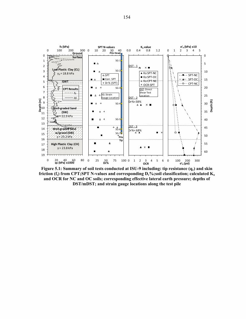
154


friction (fs) from CPT;SPT N-values and corresponding Dr%;soil classification; calculated Ko

and OCR for NC and OC soils; corresponding effective lateral earth pressure; depths of

DST/mDST; and strain gauge locations along the test pile

0 20 40 60 80

0

1

2

3

4

5

6

7

8

9

10

11

12

13

14

15

16

17

18

19

0 100 200 300

qc (kPa) x1000

De

pth

(m)

fs (kPa)

fs

qc

GWT

Low Plastic Clay (CL)γd = 18.8 kPa

Well-graded Sand (SW)

γ = 22.9 kPa

Well-graded Sand w/gravel (SW)γ = 25.2 kPa

High Plastic Clay (CH)γ = 23.8 kPa

Ground Surface

CPT Results

0 25 50 75 100

0 10 20 30 40

Dr%

SPT N-values

SPT

Corr. SPT

Dr % (SPT)

SG: Strain Gauge Location

SG-1

SG-2

SG-3

SG-4

SG-5

SG-6

SG-7

Pile Tip

Pile Head

0 1 2 3 4 5 6

0.0 0.4 0.8 1.2

OCR

Ko value

Ko SPT-NCKo SPT-OCKo CPT-NCOCR-SPT

DST - 3Dr%= 68%

DST - 2Dr%=38%

DST - 1

DST: Direct Shear Test Location

0 1 2 3 4 5

0 100 200 300

0

5

10

15

20

25

30

35

40

45

50

55

60

σ'h (kPa) x10

De

pth

(ft)

σ'h (psi)

SPT-NC

SPT-OC

CPT-NC

155


friction (fs) from CPT;SPT N-values and corresponding Dr%;soil classification; calculated Ko

and OCR for NC and OC soils; corresponding effective lateral earth pressure; depths of

DST/mDST; and strain gauge locations along the test pile

0 10 20 30

0

1

2

3

4

5

6

7

8

9

10

11

12

13

14

15

16

17

18

19

0 50 100 150 200

qc (kPa) x1000

De

pth

(m)

fs (kPa)

fs qc

GWT


γ = 17.6 kPa

Boulders

Well graded Sand w/ Gravel (SW)

γ = 23.7 kN/m3

Well-graded Gravelly Sand (SW)

γ = 23.1 kN/m3

Well-graded Sand w/Gravel (SW)γ= 24.0 kN/m3

CPT Results

Ground Surface

0 25 50 75 100

0 25 50 75 100

Dr%

SPT N-values

SPTCorr. SPTDr % (SPT)

SG-2

SG-3

SG-4

SG-5

SG-6

SG-7

SG-8

PileTip

SG: Strain Gauge Location

Pile Head

0 1 2 3 4 5 6

0.0 0.5 1.0 1.5 2.0

OCR

Ko value

Ko SPT-NCKo SPT-OCKo CPT-NCOCR-SPT

DST - 3Dr%= 76%

DST - 2Dr%=70%

DST - 1Dr%=40%

DST: Direct Shear Test Location

0 10 20 30 40 50

0 100 200 300

0

5

10

15

20

25

30

35

40

45

50

55

60

σ'h (psi)

De

pth

(ft)

σ'h (kPa)

SPT-NCSPT-OCCPTP.Cell

156

Figure 5.3: Load distribution along the pile length calculated from measured strains at different

applied loads for test site ISU-9

Figure 5.4: Measured load-displacement response at the pile head during SLT for ISU-9 and

ISU-10, and separated skin-friction and end-bearing components for ISU-9

0 25 50 75 100 125 150 175 200 225

0

10

20

30

40

50

0

2

4

6

8

10

12

14

16

0 200 400 600 800 1000

Load (kips)

De

pth

(ft

)

De

pth

(m

)

Load (kN)

42131220263353438521607678754

Load (kN)

Ground

Low Plastic Clay

Well-graded Sand w/Gravel

28% end-bearing

Well-gradedSand

0 20 40 60 80 100 120 140 160 180

0

0.1

0.2

0.3

0.4

0.5

0.6

0.7

0.8

0

2

4

6

8

10

12

14

16

18

20

0 100 200 300 400 500 600 700 800

Load (kips)

Dis

pla

cem

en

t (i

nch

)

Dis

pla

cem

en

t (m

m)

Load (kN)

Total Load (ISU-9)Skin-friction (ISU-9)End-bearing (ISU-9)Total Load (ISU-10)

157

Figure 5.5: Overview of the mDST unit as used to measure the t-z curves

Figure 5.6: Mohr-Coulomb failure envelope for the soil and the soil-pile interface obtained

using DST and mDST, respectively, at depth of 7 m forISU-9

Pnormal

Pshear

120 mm100 mm

Vertical disp.

Dial Gauge

Horizontal disp.

Dial Gauge

Shear Stress

Dial Gauge

Steel Plate

Sand

Normal Stress

Dial Gauge

20 mm

20 mm

Pressure

Lines

Pressure

Lines

Porous Plate

Porous Plate

Water Level

Loading Frame

Loading Plate

Shear Box

Upper Half

Shear Box

Lower Half

Shear Box Container

y = 0.754xR² = 0.932

y = 0.476x + 1.665R² = 0.975

0 5 10 15 20 25 30

0

5

10

15

20

25

0

20

40

60

80

100

120

0 50 100 150 200

Normal Pressure (psi)

She

ar S

tre

ss (

psi

)

She

ar S

tre

ss (

kPa)

Normal Pressure (kPa)

DST

mDSTc = 0 kPa, ф = 37o

a = 1.6 kPa, α = 25.5o


158

Figure 5.7: Comparison of t-z curves developed from mDST with those back-calculated from

strain gauges(SG)for the soil layers at test site ISU-9

Figure 5.8: Overview of the PTR unit as used to measure the q-w curves

0 0.05 0.1 0.15 0.2 0.25 0.3

0

2

4

6

8

10

12

14

16

0

20

40

60

80

100

120

0.00 1.00 2.00 3.00 4.00 5.00 6.00 7.00 8.00

Displacement (inch)

Un

it S

he

ar S

tre

ss (

psi

)

Un

it S

he

ar S

tre

ss (

kPa)

Displacement (mm)

SG 14.3m (46.9ft) mDST 13.7m (44.9ft)

SG 7.6m (24.9ft) mDST 7m (22.9ft)

SG 2.3m (7.5ft) mDST 2.5m (8.2ft)

Sand

Model

Pile

120 mm100 mm

60 mm

20 mm

25 mm

10 mm

Vertical

Dial Gauge

Normal Stress

Dial GaugePressure

Lines

Steel Bolts

Water Level

Added 20 mm Height

Spacer Plate

Loading Frame

Shear Box

Lower Half

Shear Box

Upper Half

Shear Box Container

Pnormal

Sand

Model

Pile

120 mm100 mm

60 mm

20 mm

25 mm

10 mm

Vertical

Dial Gauge

Normal Stress

Dial GaugePressure

Lines

Steel Bolts

Water Level

Added 20 mm Height

Spacer Plate

Loading Frame

Shear Box

Lower Half

Shear Box

Upper Half

Shear Box Container

Pnormal

Sand

Model

Pile

120 mm100 mm

60 mm

20 mm

25 mm

10 mm

Vertical

Dial Gauge

Normal Stress

Dial GaugePressure

Lines

Steel Bolts

Water Level

Added 20 mm Height

Spacer Plate

Loading Frame

Shear Box

Lower Half

Shear Box

Upper Half

Shear Box Container

Pnormal

Steelplate

159

Figure 5.9: FE model results representing the PTR test conducted for ISU-9

Figure 5.10: Comparison of the q-w curves obtained for the two test piles after extrapolation

from the PTR test results

0 0.05 0.1 0.15 0.2 0.25 0.3 0.35 0.4

0

2

4

6

8

10

12

0

10

20

30

40

50

60

0 1 2 3 4 5 6 7 8 9 10 11

w (inch)

q (

kip

s)

q (

kN)

w (mm)

q-w curve for ISU-9

q-w curve for ISU-10

160

Figure 5.11: Load-displacement responses based on different t-z analyses and compared with

measured response for test site ISU-9

Figure 5.12: Load distribution along the pile length calculated using TZ-T-mDST and

compared with measured values at test site ISU-9

Figure 5.13: Load-displacement responses calculated using TZ-T-mDST and compared with

measured values at test site ISU-10

0 20 40 60 80 100 120 140 160 180

0.0

0.1

0.2

0.3

0.4

0.5

0.6

0.7

0.8

0

2

4

6

8

10

12

14

16

18

20

0 100 200 300 400 500 600 700 800

Load (kips)

Dis

pla

cem

en

t (i

nch

)

Dis

pla

cem

en

t (m

m)

Load (kN)

SLT (Shaft)TZ-S-mDST (Shaft)SLT (Total)TZ-T-mDST (Total)

0 25 50 75 100 125 150 175 200 225

0

10

20

30

40

50

0

2

4

6

8

10

12

14

16

0 200 400 600 800 1000

Load (kips)

De

pth

(ft

)

De

pth

(m

)

Load (kN)

Strain GaugesTZ-T-mDST

Ground

Low Plastic Clay


Well-gradedSand

0 20 40 60 80 100 120 140 160

0

0.1

0.2

0.3

0.4

0.5

0.6

0.7

0.8

0

2

4

6

8

10

12

14

16

18

20

0 100 200 300 400 500 600 700

Load (kips)

Dis

pla

cem

en

t (i

nch

)

Dis

pla

cem

en

t (m

m)

Load (kN)

SLT (Total)TZ-T-mDST (Total)

161

CHAPTER 6: PILE RESPONSE CHARACTERIZATIONUSING A FINITE

ELEMENT APPROACH


2; Muhannad T. Suleiman, M. ASCE

3

A paper to be submitted to a conference proceeding

6.1. Abstract

The study presented herein focused on improving the accuracy and efficiency of

simplified two-dimensional finite element (FE) models in simulating the response of

vertically-loaded steel piles driven into cohesive and cohesionless soils. For this purpose,

data from four static load tests (SLTs) conducted on instrumented steel H-piles driven into

clay and sand soil profiles accompanied by various in-situ and laboratory soil tests were

used. The behavior of the load-tested piles was simulated using axisymmetric FE analyses,

based on the Mohr-Coulomb soil constitutive model by means of PLAXIS 7.2. Following

identification that the elastic modulus of cohesive soils and the soil-pile interface properties

are poorly represented in the analysis, these capabilities were improved first. The modulus of

clay soil was obtained from a Consolidated Undrained (CU) Triaxial soil laboratory test,

while the modified Direct Shear Test (mDST) was utilized to provide an accurate laboratory

measurement of the soil-pile interface properties. With these refinements, the FE model

provided an improved prediction for the load-displacement response of the four test piles

without using sophisticated soil constitutive models that require conducting costly and time

consuming tests.

Keywords: Finite Element; Pile Foundations; Soil-structure Interaction; Load-displacement;

Interface Element; Soil Elastic Modulus.



Engineering, Iowa State University, 376 Town Engineering, Ames, IA 50011-3232, E-mail: [email protected] 3 Assistant Professor, Dept. of Civil and Environmental Engineering, Lehigh University, STEPs

Building, Room 326, 1 West Packer Avenue, Bethlehem, PA, 18015. E-mail: [email protected]




162

6.2. Introduction

An analysis approach to predict the load-displacement response of axially-loaded

piles can facilitate incorporation of both strength and serviceability limit states in routine

design of deep foundations. According to Guo and Randolph (1998), analytical methods used

to characterize pile behavior can be classified into three major categories: (1) approximate

closed-form solutions, (2) one-dimensional numerical algorithms, and (3) boundary or finite

element methods. The first two categories depend on load-transfer analysis, an iterative

technique for solving the nonlinear differential equations of load-transfer using the finite-

difference method (Coyle and Reese, 1966; Suleiman and Coyle, 1976). The third category

depends on a more comprehensive modeling technique and accurate characterization of

material behavior.

Recently, numerous studies have successfully adapted the load-transfer analysis (t-z

analysis) to model the pile behavior under axial loads (Misra and Chen, 2004; Misra and

Roberts, 2006; Roberts et al., 2008; AbdelSalam et al., 2010). Although the t-z analysis

provides the load-displacement response at the pile head and load transfer as a function of

pile depth, it does not provide the stresses and strains induced in the surrounding soil

medium. Consequently, the t-z method may not provide insight into the response of soil and

pore water pressure development around the pile (Wathugala and Desai, 1989). The

repercussion of not having this knowledge is that the influence of the load transferred

through one pile on adjacent piles in a pile group or nearby shallow or deep foundations may

not be known. In these cases, it is important to use a detailed model to examine the load

transfer in a pile. For vertically-loaded piles, the soil properties and the interface element

behavior are the most important parameters that control the accuracy of the finite element

(FE) analysis outcomes. More specifically, De-Gennaro et al. (2006) and Engin et al. (2007)

reported soil-pile interface properties and the soil modulus typically estimated, based on

empirical correlations, largely dictate FE analysis results. Therefore, utilizing more detailed

laboratory tests to obtain the soil constitutive properties may be appropriate (De-Gennaro et

al., 2006; Engin et al., 2007). The accuracy of the FE analysis results is also dependent on the

pile material and construction techniques (El-Mossallamy, 1999).

The objective of this study is to examine the accuracy and efficiency of a simplified

163

Mohr-Coulomb soil constitutive model in simulating the response of vertically-loaded steel

H-piles driven into cohesive and cohesionless soils by utilizing a two-dimensional

axisymmetric FE analysis using PLAXIS 7.2. For this purpose, data from four vertical static

load tests (SLTs) conducted on instrumented steel H-piles accompanied with various in-situ

and laboratory soil tests were used. In the preliminary FE analysis, the soil constitutive

parameters were estimated, based on empirical correlations with Cone Penetration Test

(CPT) data. Two parameters were determined to represent the main potential sources for

error in the FE model. These two parameters were the soil-pile interface properties and the

soil elastic modulus. To improve the determination of these parameters, the soil-pile interface

properties were measured in the laboratory using a modified Direct Shear Test (mDST),

which directly measures the shear stress versus displacement relationship at soil-steel

contacts without the use of empirical correlations. In addition, the soil elastic modulus was

measured by means of a Consolidated Undrained (CU) Triaxial soil test. Measured soil

constitutive properties were used in the FE model, which showed significant improvement in

predicting the pile load-displacement behavior compared with the field measured responses

of the four load tested piles. A significant benefit of improving the simplified FE model is

that it can facilitate incorporation of the vertical settlement and serviceability limits into the

design of deep foundations.

6.3. Preliminary FE Model

For soil-structure interaction problems, the commercially-available finite element

code, PLAXIS, has been widely used and reported by many researchers to model the

behaviour of deep foundations with an acceptable accuracy (Prakoso and Kulhawy 2001;

Sellountou et al., 2005; Oh et al., 2008). In this study, PLAXIS was used because it is

capable of solving non-linear plasticity problems using a ―staged construction‖ operation,

which allows for changing the load configuration on the model pile head, pore water pressure

distribution, and pile geometry. Ideally, a three-dimensional analysis is preferable to simulate

the behaviour of steel H-piles, but as iterated before, this is the first attempt to analyze steel

H-piles using a simplified axisymmetric model in sand and clay soils. The H-pile was

represented in the axisymmetric model assuming the cross-section of the actual pile is

164

circular. However, the model pile diameter was selected to provide the same surface area of

the actual H-pile along the shaft, while the cross-section of the model pile was gradually

reduced at the tip to reflect the actual area of the pile‘s tip. The H-pile was modeled using a

non-porous linear-elastic constitutive model with properties summarized in Table 6.1. To

eliminate the effects of the FE model vertical boundaries on the soil-pile response, the model

diameter was selected equal to 7.0D, where D is the model pile diameter. Also, a length equal

to 5D was defined between the model pile tip and the bottom horizontal boundary of the FE

model.

The preliminary FE analysis was conducted to model the behavior of four statically

load tested piles. Two of the test piles with identification numbers (ISU-4 and ISU-5) were

driven into cohesive soil layers and the other two test piles (ISU-9 and ISU-10) were driven

into mainly cohesionless soil layers. Table 6.1 summarizes soil layers and soil properties for

all test sites. As can be seen in the table, the unit weights of different soil layers were

measured in the laboratory, while the remaining soil constitutive parameters were estimated

using correlations with the CPT results. All the empirical correlations with the CPT data used

to estimate the soil properties are referenced in Table 6.1. In all cases, the Mohr-Coulomb

model was used to describe the constitutive soil behavior utilizing an unstructured very fine

mesh consisting of 15-node triangular elements. The Mohr-Coulomb elastic perfectly plastic

model was selected for this preliminary FE analysis because it is one of the most widely used

constitutive models and has proven to be quite accurate and efficient in simulating soil-

structure interaction problems (Tan and Bui, 2006). In addition to the elastic soil modulus

and Poisson‘s ratio, Es and ν, respectively, the Mohr-Coulomb model incorporates the use of

three plastic parameters, φ, c, and ψ, which denote the friction angle, cohesion, and dilatancy

angle of the soil material, respectively. The angle of dilatancy can be defined as the tendency

of soil to expand in volume due to shear. Table 6.1 includes all the required soil constitutive

parameters for this analysis based on the Mohr-Coulomb model.

In the preliminary FE models, the ground water table was defined for all test sites,

using the phreatic surface option of the program and the initial stresses were generated using

the predefined Ko values based on the friction angle of the soil. For the interface element

between the soil and the pile, the PLAXIS code uses a virtual zero thickness element with

165

reduced properties that connect pile elements with surrounding soil elements. The reduced

interface properties are defined for each soil layer by determining the strength reduction

factor for interfaces (Rinter). This factor relates the strength of the interface (in terms of

friction angle, α, and adhesion, a) to the soil cohesion and friction angle. Based on the

PLAXIS user manual recommendations, the Rinter can be assumed equal to 0.50 and 0.67 for

clay-steel and sand-steel contacts, respectively. Table 6.1 summarizes the used values of the

Rinter in the preliminary FE analysis for different soil layers presented at the four test sites.

Table 6.1: Constitutive soil parameters estimated using empirical correlations to CPT

Test

Site

Soil

Layers(1) Thickness

m γdry

kN/m3

γwet

kN/m3 Su

(2)

kPa c(3)

kPa ϕ(4) ν(5)

Es(6)

kPa Rinter

ISU-4

(GWT:

4.5m)

Clay 0 - 1.5 17 21.3 101 50 34 0.3 9347 0.5

Clay 1.5 - 5.5 18.2 21.3 102 51 29 0.25 10586 0.5

Clay 5.5 - 11 18.9 21.3 177 88 33 0.35 13662 0.5

Clay 11 - 18 19.5 22.4 129 64 31 0.35 10366 0.5

ISU-5

(GWT:

10.0m)

Clay 0 - 7.6 17.5 21.1 107 54 32 0.30 9753 0.5

Clay 7.6 - 12 19.5 22.9 148 74 32 0.30 13638 0.5

Clay 12 - 18 20.5 23.8 180 90 34 0.35 16464 0.5

ISU-9

(GWT:

5.2 m)

Clay 0 - 4.8 18.8 23.4 216 108 34 0.25 17070 0.5

Sand 4.8 - 13 18.5 22.9 0 0 40 0.45 28560 0.67

Sand 13- 16 21.4 25.2 0 0 44 0.45 19490 0.67

ISU-10

(GWT:

3.0 m)

Sand 0 - 4.6 17.6 20.2 0 0 36 0.45 9248 0.67

Sand 4.6 - 15 20.3 24.0 0 0 40 0.45 24390 0.67

Boulder 15 -17 24 24.0 0 0 44(7) 0.25 270000(7) 0.67


3; and 1 kPa = 0.145 psi.

(1) An undrained soil condition was used for the cohesive layers, while a drained condition was used

for cohesionless layers; (2)

After Schmertmann et al. (1978) using Nk = 15; (3)

c = Su/2; (4)

After

Robertson and Campanella (1983); (5)

After Das (1998); (6)

After Mayne and Kulhawy (1990) using

M=8.25 (qt-ζvo); and(7)

CPT not available, ϕ and Es were extrapolated. Pile: Linear-Elastic model;

γ=50 kN/m/m; Es=2.0E8 kPa; υ=0.2; Shaft radius=0.16m; Tip radius=0.05m; Rinter=1.0.Steel Plate:

Elastoplastic model; EA=1.6x10E8 kN/m; EI=9000 kN m2/m; d=0.026m; w=0.57 kN/m/m; υ=0.25.

6.3.1. Piles in cohesive soils

The two test piles referred to as ISU-4 and ISU-5 were selected for the preliminary

FE analysis in cohesive soils. Figure 6.1a shows different soil layers, boundary conditions,

and the interface elements used along the pile length for the preliminary FE model

representing the test pile ISU-4 (FE-ISU4-1 model). As can be seen from the figure, the

bottom boundary was totally fixed in both directions, while the side boundaries were only

166

fixed in the horizontal direction. The figure also shows the positive interface elements

connecting the soil and pile elements along different soil layers. The positive interface means

the interface is connecting the outer surface of the pile with the soil. Figure 6.1b shows a

view of finite element mesh generated for this analysis.

Figure 6.1: FE model representing the test pile at ISU-4

The FE analysis was performed based on controlled vertical displacement increments

that represented the same displacement values collected during the static load test on the test

piles. Using the staged construction option of the program, the displacements and stresses

were reset for each loading increment to avoid convergence issues that could take place in

the analysis. For the FE-ISU4-1 model, Figures 6.2a and 6.2b, respectively, show the

deformed mesh and the distribution of the total displacement corresponding to an extreme

prescribed vertical displacement of 40 mm (1.6 inch) at the model‘s pile head. As can be seen

from the figure, the maximum total displacement around the model‘s pile was limited to

around 2.5D, where D is the model pile diameter; hence, the FE model boundaries had no

effect on total displacement. Moreover, Figure 6.2c shows the plastic zone by means of the

effective normal stresses developed in the soil medium at the extreme total displacement. As

can be seen from the figure, the maximum effective normal stress induced in the soil is 410.6

kPa (59.6 psi), concentrated at an approximate distance of around 3D below the pile tip and

degrading towards the bottom horizontal boundary. Thus, the bottom boundary has a

(a) Model overview (b) Fine unstructured mesh

167

negligible effect on the stresses induced in the soil below the pile tip.

Figures 6.3a and 6.3b show the predicted load-displacement response at the pile head

compared to the measured response for the test piles ISU-4 and ISU-5, respectively. From

Figure 6.3a, it can be seen the predicted load-displacement curve is less stiff by about 60%

compared to the measured response along the elastic portion. Moreover, the predicted load-

displacement curve underestimated the pile nominal capacity at the plastic portion by 43%

when compared with the measured pile nominal capacity. For each case, the measured pile

nominal capacity was defined using the Davisson criterion (Davisson, 1972) represented in

the figures by a dot line referred to as the Davisson line. For the FE model that represented

the test pile ISU-5 (FE-ISU5-1 model), Figure 6.3b shows the predicted load-displacement

curve has stiffness 64% less than that of the measured curve along the elastic portion, and

65% lower nominal capacity compared to the measured capacity. Thus, the preliminary FE

analyses for vertically-loaded piles driven into cohesive soils generally show poor

correlations compared to field measured responses. The previous conclusion was expected,

as several studies reported estimated soil-pile interface properties and soil elastic modulus,

based on empirical correlations that could lead to biased FE results (El-Mossallamy 1999;

De-Gennaro 2006; Engin 2007).

Figure 6.2: FE model results for the test pile at ISU-4

168

Figure 6.3: Predicted versus measured pile load-displacement responses for piles in clay

6.3.2. Piles in cohesionless soils

The same axisymmetric FE model was utilized to simulate the behavior of the other

two test piles driven into mainly cohesionless soil layers and referred to as ISU-9 and ISU-

10. However, the top soil layer at ISU-9 was classified as low plastic clay with thickness

equal to 4.8m (15.74 ft). As summarized in Table 6.1, all the constitutive parameters were

established for the soil material, based on empirical correlations to the CPT conducted at

each test site. This table also summarizes the selected Rinter values for each soil layer, based

on the recommended values in the PLAXIS user manual. Figure 6.4a shows different soil

layers, boundary conditions, and the interface elements used along the pile length for the

preliminary FE model representing ISU-9 (FE-ISU9-1 model). Moreover, Figure 6.4b shows

a view of finite element mesh used for the analysis.

For the FE-ISU9-1 model, Figures 6.5a and 6.5b, respectively, show the deformed

mesh and the distribution of the total displacement corresponding to the extreme prescribed

vertical displacement of 18.4 mm (0.72 inch) at the model‘s pile head. As can be seen from

Figure 6.5a, the maximum total displacement around the model‘s pile was concentrated in

the top clay layer and below the model‘s pile tip. However, the displacement did not extend

laterally more than around 5.0D. Hence, the FE model boundaries had minimal effects on

total displacements. Moreover, Figure 6.5c shows the plastic zone by means of effective

normal stresses developed in the soil medium at the extreme total displacement. As seen in

this figure, the maximum effective stress induced in the soil is 421.9 kPa (61.2 psi), which is

0 20 40 60 80 100 120 140 160 180

0

0.2

0.4

0.6

0.8

1

1.2

1.4

1.6

1.8

0

5

10

15

20

25

30

0 100 200 300 400 500 600 700 800

Load (kips)

Dis

pla

cem

en

t (i

nch

)

Dis

pla

cem

en

t (m

m)

Load (kN)

SLT (ISU4)

FE-ISU4-1

0 40 80 120 160 200 240 280

0

0.2

0.4

0.6

0.8

1

1.2

1.4

1.6

1.8

0

5

10

15

20

25

30

35

0 200 400 600 800 1000 1200

Load (kips)

Dis

pla

cem

en

t (i

nch

)

Dis

pla

cem

en

t (m

m)

Load (kN)

SLT (ISU5)

FE-ISU5-1

(b) Test pile at ISU-5 (clay)(a) Test pile at ISU-4 (clay)

169

concentrated directly below the model pile tip and degrading towards the bottom horizontal

boundary.

Figure 6.4: FE model representing the test pile at ISU-9

Figure 6.5: FE model results for the test pile at ISU-4

From Figure 6.6a, it can be seen that the predicted load-displacement curve using the

FE-ISU9-1 model is about 41% less stiff than the field measured response along the elastic

(a) Model overview (b) Fine unstructured mesh

170

portion. However, the predicted ultimate capacity of the pile was about 26% conservative

compared to the measured nominal capacity using Davisson‘s criterion. This difference

between the predicted and the measured responses for ISU-9 could be due to the top clay

layer at the test site. For the FE model representing the test pile ISU-10 (FE-ISU10-1 model),

Figure 6.6b shows a relatively better prediction of the load-displacement curve along the

elastic and plastic portions compared to the field measured pile response. The observation

here is the FE model provided a very good match with the actual measurements for the test

pile ISU-10 (pile driven into sand soil layers), which is relatively better compared with the

predicted behaviors for the test pile ISU-9 (pile driven into mainly sand layers with one clay

layer at the top) and the test piles ISU-4 and ISU-5 (piles driven into clay soil layers).

Therefore, it is obvious the FE model prediction for the load-displacement behavior is better

in the case of piles driven into cohesionless soil layers compared to those predicted for piles

driven into cohesive soil layers.

Figure 6.6: Predicted versus measured pile load-displacement responses

6.4. Investigation of the Soil and Interface Properties

As previously indicated, the bias in the FE analysis results in the case of piles driven

into cohesive soils could be due to: 1) the use of inappropriate interface based on general

recommendations from the PLAXIS user manual and 2) the subjective estimate of the soil

elastic modulus based on empirical correlations to CPT results. In this section, the effect of

changing the properties of the soil-pile interface element was first studied separately in the

0 20 40 60 80 100 120 140 160 180

0

0.1

0.2

0.3

0.4

0.5

0.6

0.7

0.8

0

2

4

6

8

10

12

14

16

18

20

0 100 200 300 400 500 600 700 800

Load (kips)D

isp

lace

me

nt

(in

ch)

Dis

pla

cem

en

t (m

m)

Load (kN)

SLT (ISU10)FE-ISU10-1

0 20 40 60 80 100 120 140 160 180

0

0.1

0.2

0.3

0.4

0.5

0.6

0.7

0.8

0

2

4

6

8

10

12

14

16

18

20

0 100 200 300 400 500 600 700 800

Load (kips)

Dis

pla

cem

en

t (i

nch

)

Dis

pla

cem

en

t (m

m)

Load (kN)

SLT (ISU9)FE-ISU9-1

(b) Test pile at ISU-10 (sand)(a) Test pile at ISU-9 (sand + clay)

171

case of cohesive soils. After this, the soil modulus was measured in the laboratory for clay.

The difference between the measured and predicted values of the soil modulus was used in

the final FE model to improve the analysis as will be discussed in the next sections.

6.4.1. Interface properties

Recently, AbdelSalam et al. (2010) modified the Direct Shear Test (mDST) to

measure the shear-displacement curves, or the t-z curves that represent the soil-pile interface

properties, by shearing a steel plate with respect to soil within the direct shear box. The

accuracy of the soil-steel interface response for clay soils was first investigated in PLAXIS

by examining the reproducibility of the mDST test data. For this purpose, a plane strain two-

dimensional FE model was adapted, where the steel plate of the mDST was modeled using a

non-porous linear-elastic constitutive model. The soil medium was modeled using the Mohr-

Coulomb constitutive model, where the soil shear strength properties were determined, based

on actual laboratory measurements from a conventional Direct Shear Test (DST) conducted

on the sample collected from the top clay layer for ISU-9. The soil elastic modulus for clay

was determined, based on CPT test results, while the only changeable parameter was the

Rinter along the contact surface between the soil and the steel plate. The values of the Rinter

used in the analysis were equal to 0.3, 0.4, 0.5, and 0.7. Table 6.2 summarizes the soil and

interface parameters used in the four FE models representing the mDST test conducted for

the clay layer from ISU-9.

As shown in Figure 6.7a, a constant vertical normal stress was applied on top of the

soil during the FE analysis. Controlled horizontal displacement increments were applied to

the lower half of the shear box, following the same normal stress and horizontal

displacements collected while conducting the mDST laboratory test. Figure 6.7a also shows

the plastified zone by means of the effective normal stresses developed in the soil medium,

due to an applied constant normal stress of 30 kPa (4.35 psi) and horizontal displacement of

10 mm (0.4 inch) to the lower half of the shear box, and that for the FE model ISU-9/3. As

seen from the figure, the maximum normal effective stress induced in the soil was equal to

14.44 kPa (2.09 psi), concentrated at the interface between the upper and lower shear boxes

with higher intensity towards the vertical boundaries. Furthermore, Figure 6.7b represents the

172

shear stresses induced along the interface element, indicating a maximum shear stress value

of 15.40 kPa (2.23 psi).

Figure 6.8 represents the shear stress-displacement curves adapted from the FE

models for the clay soil sample using different Rinter values and compared with the measured

curve from the mDST laboratory test. From Figure 6.8, it was found that: 1) Rinter equal to 0.5

better represents the behavior at the clay-steel interface, indicating the recommended value in

the PLAXIS user manual is appropriate; and 2) the effect of the changing the Rinter was not

significant on the shear-displacement response, when it exceeded a value of 0.5. From

previous observations, it is clear the interface element in PLAXIS is considered acceptable in

the case of clay-steel contacts. Therefore, bias in results of the FE model representing

axially-loaded steel pile driven into clay could be due to improper estimates of the soil elastic

modulus, not the soil-pile interface properties. Thus, the soil modulus significantly controls

the soil-pile behavior and needs to be investigated separately.

Table 6.2: Summary of the soil parameters, and Rinter values used in the sensitivity analysis for

the soil-steel interface

Model ID Soil

type

P

kPa

γdry

kN/m3

γwet

kN/m3

c(1)

kPa ϕ(1) ν(2)

Es(3)

Rinter kPa

ISU-9/1 mDST

test for

Clay

30 18.8 23.4 10 24 0.25 Es=17070

0.3

ISU-9/2 0.4

ISU-9/3 0.5

ISU-9/4 0.7

ISU-5-CPT Triaxial

test for

Clay

120 17.5 21.1 54 32

0.3 E1=9753 Not

used ISU-5/1 0.3 E2=14629

ISU-5/2 0.3 E3=19506

For unit conversion: 1 kN/m3 = 6.24 lb/ft

3; and 1 kPa = 0.145 psi.

(1) Measured, using the DST results in the case of FE models for ISU-9, and estimated based on CPT

results in the case of FE models for ISU-5; (2)

Estimated, based on Das (1998); and (3)

Es and E1 were

estimated using CPT data based on correlations after Mayne and Kulhawy (1990), where E2 = E1 x 1.5,

and E3 = E1 x 2.

173

Figure 6.7: FE model representing the mDST test for clay soils

Figure 6.8: Comparison between the shear stress-displacement curves adapted from the FE

models using different Rinter values and the laboratory measured curve using the mDST for clay

6.4.2. Soil modulus

Empirical correlations for estimating the soil modulus from the CPT results, such as

the equation provided by Mayne and Kulhawy (1990), are not complex, and settlements can

be estimated relatively quickly from these correlations. However, Lunne and Powell (1997)

indicated the estimation of drained consolidation or deformation parameters, such as the

constrained modulus, M, and Young‘s Modulus, Es, for cohesive soils, based on the

undrained CPT test results, may lead to serious errors by as much as ± 100%, especially

when based on empirical correlations from the literature. Abu-Farsakh and Titi (2004)

indicated that using the CPT test results to estimate the Es requires extensive work to

determine which correlation is the most appropriate to use. However, with local experience

individual site/area specific correlations can be developed for certain soil types with greater

0.00 0.05 0.10 0.15 0.20 0.25 0.30 0.35 0.40

0.0

0.5

1.0

1.5

2.0

2.5

3.0

0

3

5

8

10

13

15

18

20

0 1 2 3 4 5 6 7 8 9 10

Displacement (inch)

She

ar S

tre

ss (

psi

)

She

ar S

tre

ss (

kPa)

Displacement (mm)

mDSTFE-1 (R=0.3)FE-2 (R=0.4)FE-4 (R=0.5)FE-4 (R=0.7)Clay Sample

174

reliability.

In this study, a CU triaxial test was conducted on an undisturbed clay soil sample

collected at a depth of 7.0 m (23 ft) below ground surface from the test site at ISU-5. A

confining stress of 120 kPa (17.4 psi), estimated to represent the effective lateral earth

pressure in the field, was used to consolidate the sample. As presented in Figure 6.9, the

stress-strain curve was measured and the soil maximum effective stress was around 135 kPa

(19.6 psi) and the elastic soil modulus was around 40000 kPa (5801.5 psi). However, the

direct use of measured value of the soil modulus in the FE model may still not yield the same

measured stress-strain behavior. This is because there are several other factors and

parameters that affect FE analysis in addition to the soil modulus. Thus, to improve the FE

model to match the actual measured stress-strain response from the CU triaxial test, an

investigation that addresses the effect of changing the soil modulus on the overall stress-

strain behavior was conducted for the clay soil sample. The objective for this analysis was to

determine an adjustment factor that needs to be multiplied by the typically estimated soil

modulus using empirical correlations with CPT data and to improve the overall FE model

results for similar soil and pile conditions.

For the first model in this sensitivity analysis (ISU-5-CPT model), soil strength, and

elastic modulus were calculated, based on empirical correlations with the soil CPT test

results previously presented in Table 6.1. An axisymmetric FE model was adapted to

simulate the behavior of the soil sample inside the CU triaxial chamber. The FE model was

conducted using 10 controlled vertical displacement increments, but before running the load

increments, the soil was consolidated using the Automatic Time Stepping (ATS) option from

the PLAXIS program. In ATS analysis, the program uses smaller time steps while applying

the confinement stress until the soil sample is fully consolidated. Figures 6.10a and 6.10b,

respectively, show the deformed mesh of the soil sample and the distribution of the total

displacement corresponding to the maximum prescribed vertical displacement of 0.2 mm

(0.008 inch) that represents a vertical strain of about 0.15%. Furthermore, Figure 6.10c

shows the plastic zone by means of the effective normal stresses developed in the soil

medium, with a maximum value equal to around 157 kPa (22.77 psi) at the maximum

prescribed displacement. On the other hand, Figure 6.11 shows the predicted stress-strain

175

curve, limited to an elastic strain of about 0.2%, adapted from the ISU-5-CPT model, and

compared to the laboratory measured curve using the CU-triaxial test. As seen from the

figure, the difference between the slope of the predicted and measured stress-strain curves is

about 41%. Therefore, the predicted Es, based on empirical correlations using CPT, may be

misleading in case of clay soils. This was expected, according to several previous studies

conducted by Mayne and Kulhawy (1990), Lunne and Powell (1997), and Abu-Farsakh and

Titi (2004).

To improve the estimation of the soil elastic modulus used in the FE model to match

the laboratory measured results, two additional models were adapted (ISU-5/1 and ISU-5/2)

using increased Es values by 50 and 100%, respectively, compared to the previously

estimated values from the CPT. All soil parameters used in the FE models are summarized in

Table 6.2. The results from ISU-5/1 and ISU-5/2 are presented in Figure 6.11, which shows

the stress-strain curve adapted using the doubled Es matches the initial portion of the

measured curve at low strain levels (i.e., strain less than 0.2%). Hence, the estimated values

for the initial elastic modulus of clay soils, based on empirical correlations to the CPT test

results, must be increased by 100%.

Figure 6.9: Stress-strain curve from the CU-triaxial results for the soil sample at ISU-5

0.00 0.05 0.10 0.15 0.20 0.25 0.30

0

2

4

6

8

10

12

14

16

18

20

22

0

20

40

60

80

100

120

140

160

0.00 0.50 1.00 1.50 2.00 2.50 3.00

Strain %

Effe

ctiv

eD

evi

ato

r St

ress

(p

si)

Effe

ctiv

e D

evi

ato

r St

ress

(kP

a)

Strain %

CU-Triaxial

176

Figure 6.10: FE model for the CU-triaxial test conducted on a clay soil sample

Figure 6.11: Stress-strain curve from different FE models and the triaxial test

6.5. Improved FE Models

This section presents an improved FE analysis for modeling the axially-loaded piles

embedded in cohesive soil layers. This was attained by addressing the bias in the values of

the estimated elastic modulus of clay soil layers, based on CPT data, increased by 100%

based on laboratory CU-Triaxial measurements. However, the interface properties were

found appropriate, and were not changed in the improved analysis. Out of the four test sites

previously modeled (i.e., ISU-4, ISU-5, ISU-9, and ISU-10), three sites contained clay layers.

0.00 0.03 0.05 0.08 0.10 0.13 0.15 0.18 0.20

0

1

2

3

4

5

6

7

8

9

10

11

12

0

10

20

30

40

50

60

70

80

0.00 0.03 0.05 0.08 0.10 0.13 0.15 0.18 0.20

Strain %

Effe

ctiv

e S

tre

ss (

psi

)

Effe

ctiv

e S

tre

ss (

kPa)

Strain %

CU-triaxialISU-5-CPTISU-5/1ISU-5/2

177

Accordingly, the soil elastic modulus used for clay layers in the FE models for ISU-4, ISU-5,

and ISU-9 were adjusted by doubling the previously estimated values of Es based on CPT

data.

The analysis was first conducted for the two test piles embedded in mainly clay soil

layers at ISU-4 and ISU-5. As seen from Figure 6.12a that represents test pile ISU-4, the

difference within the elastic portion of the load-displacement curves predicted, using the

earlier FE model (FE-ISU4-1) and the improved model (FE-ISU4-2), was reduced from 60%

to 27%, compared to the measured response. Moreover, using the improved model reduced

the difference between the predicted and measured pile ultimate capacity using Davisson‘s

criterion from 43 to 11%. This significant enhancement in the estimated load-displacement

behavior of test pile ISU-4 was attained after using the correct value of the soil modulus for

clay layers. For pile ISU-5, the difference between the predicted and measured load-

displacement responses was reduced from 64 to 33% along the elastic portion of the curve,

and from 65 to 9% at the ultimate capacity, based on Davisson‘s criterion (see Figure 6.13b).

Hence, the improved FE models for both test sites satisfactorily simulated the behavior of the

test piles embedded in mainly cohesive soil layers.

As previously indicated, the FE model used to simulate the behavior at ISU-10 has

provided an accurate prediction of load-displacement response for the axially load tested pile

embedded in sand soil layers. However, this was not the case for the test pile at ISU-9

embedded in sand and clay soil layers. Accordingly, an improved FE model (FE-ISU9-2)

with doubled soil elastic modulus for the top clay layer at ISU-9 was used. As can be seen

from Figure 6.14a, the differences between the predicted and measured load-displacement

responses for the test pile at ISU-9 was reduced from 41 to 30% along the elastic portion of

the curve, and from 26 to 7.5% at the ultimate capacity based on Davisson‘s criterion. To

confirm this improvement in the FE model prediction, the load distribution along the pile

length was also adapted from the model‘s results and compared to the measured response,

based on the strain gauges data. Figure 6.14b provides the measured versus the predicted load

distribution curves along the pile length from ISU-9. From this figure, it is obvious the

improved FE model satisfactorily simulated the load distribution along the pile embedment

length in different soil layers.

178

Figure 6.12: Load-displacement behavior using the preliminary and improved FE models

versus the measured response

Figure 6.13: Pile behavior at ISU-9 using the preliminary and improved FE models versus the

measured response


A simplified two-dimensional axisymmetric FE analysis using Mohr-Coulomb soil

constitutive model was utilized to simulate the behavior of four load tested steel H-piles

using PLAXIS 7.2. The soil constitutive properties were first established, based on empirical

correlations to the CPT data. A preliminary analysis showed the model can adequately

characterize the behavior of the steel piles driven into cohesionless soil layers. However, the

model did not accurately capture the load-displacement response for the piles driven into

cohesive layers. The properties of the soil-pile interface element and the soil elastic modulus

were investigated using the mDST and CU-Triaxial soil laboratory tests, respectively, aimed

0 20 40 60 80 100 120 140 160 180

0

0.2

0.4

0.6

0.8

1

1.2

1.4

1.6

1.8

0

5

10

15

20

25

30

0 100 200 300 400 500 600 700 800

Load (kips)

Dis

pla

cem

en

t (i

nch

)

Dis

pla

cem

en

t (m

m)

Load (kN)

SLT (ISU4)FE-ISU4-1FE-ISU4-2

0 40 80 120 160 200 240 280

0

0.2

0.4

0.6

0.8

1

1.2

1.4

1.6

1.8

0

5

10

15

20

25

30

35

0 200 400 600 800 1000 1200

Load (kips)

Dis

pla

cem

en

t (i

nch

)

Dis

pla

cem

en

t (m

m)

Load (kN)

SLT (ISU5)FE-ISU5-1FE-ISU5-2

(b) Test pile at ISU-5(a) Test pile at ISU-4

0 25 50 75 100 125 150 175 200 225

0

10

20

30

40

50

0

2

4

6

8

10

12

14

16

0 200 400 600 800 1000

Load (kips)

De

pth

(ft)

De

pth

(m)

Load (kN)

SLT FE-ISU9-1FE-ISU9-2

Ground

Plastic Clay


28% end-bearing

Well-gradedSand

24% end-bearing

0 20 40 60 80 100 120 140 160 180

0

0.1

0.2

0.3

0.4

0.5

0.6

0.7

0.8

0

2

4

6

8

10

12

14

16

18

20

0 100 200 300 400 500 600 700 800

Load (kips)

Dis

pla

cem

en

t (i

nch

)

Dis

pla

cem

en

t (m

m)

Load (kN)

SLT (ISU9)

FE-ISU9-1

FE-ISU9-2

(b) Load-distribution along the pile length(a) Load-displacement

179

at improving the overall FE model results. A summary of the major findings is presented

below.

The preliminary FE model provided adequate prediction of the load-displacement

response for the test pile driven into sand soil layers at ISU-10. The preliminary

FE analysis for the pile at ISU-9, embedded in sand and clay soil layers, provided

a 41% softer load-displacement response along the elastic portion of the curve and

a 26% lower pile capacity. However, the FE models for the test piles ISU-4 and

ISU-5 driven into clay soil layers provided biased results.

The interface investigation showed a value of 0.5 for the Rinter factor should be

used to represent the soil-pile interface element properties in PLAXIS for clay-

steel contacts.

The soil modulus investigation showed the estimated elastic modulus, based on

empirical correlations with the CPT results for clay soils, was underestimated by

100%. Based on the CU-Triaxial test measurements; the estimated value of the

elastic modulus was increased by 100% for all clay layers to improve the FE

models for ISU-4, ISU-5, and ISU-9.

The improved FE model for ISU-4 showed the differences between the predicted

and measured load-displacement responses were reduced from 60 to 27% along

the elastic portion of the curve, and from 43 to 11% at the ultimate capacity. For

ISU-5, the difference between the predicted and measured load-displacement

responses was reduced from 64 to 33% along the elastic portion of the curve, and

from 65 to 9% at the ultimate capacity. For ISU-9, the difference between the

predicted and measured load-displacement responses was reduced from 41 to 30%

along the elastic portion of the curve and from 26 to 7.5% at the ultimate capacity.

Overall, the improved FE model provided satisfactory results compared with the

field measurements for the tested piles. The improved FE analysis is based on the

simple Mohr-Coulomb constitutive model, which avoids using sophisticated soil

models that require conducting costly and time consuming soil tests.

180




Foundations in Iowa funded by the Iowa Highway Research Board (IHRB). The authors

express their gratitude to the IHRB and members of the project Technical Advisory

Committee for their guidance and advice. The members of this committee represent Office of

Bridges and Structures, Soils, Design Section, and Office of Construction of the Iowa DOT,

FHWA Iowa Division, and Iowa County Engineers. Finally, special thanks to Kam Weng Ng

and Matthew Roling for their help during field/laboratory tests.

6.8. References

AbdelSalam, S. S., Suleiman, M. T., and Sritharan, S. (2010). ―Improved t-z Analysis for

Vertically Loaded Piles in Cohesionless Soils based on Laboratory Test

Measurements.‖ To be submitted to the ASCE Journal of Geotechnical and

Geoenvironmental Engineering (July 2010).

Abu-Farsakh, M. Y. and Titi, H. H. (2004). ―Assessment of Direct CPT Methods for

Predicting the Ultimate Capacity of Friction Driven Piles.‖ ASCE Journal of

Geotechnical and Geoenvironmental Engineering, volume 130, No. 9, pp. 935 - 944.

ASTM D4767 (2004). ―Standard Test Method for Consolidated Undrained Triaxial

Compression Test for Cohesive Soils.‖ doi:10.1520/D4767-0.



Das B. M. (1998). ―Principles of foundation engineering.‖ 4th

edition, PWS publishing Inc.



De-Gennaro, V., Said, I., and Frank, R. (2006). ―Axisymmetric and 3D Analysis of Pile Test




Over-consolidated Clay.‖Proceeding: The 7th

International Symposium on Numerical

http://en.wikipedia.org/wiki/Digital_object_identifier

http://dx.doi.org/10.1520%2FD4767-04

181

Models in Geotechnical Engineering, September 1999, 433-450. Rotterdam,

Balkema.


Elements for the Modeling of Piles.‖ Proceeding: The 10th

International Symposium

on Numerical Models in Geotechnical Eng. – NUMOG X, Rhodes (Greece).

Guo, W. D. and Randolph, M. F.(1998). ―Vertically Loaded Piles in Non-homogeneous

Media.‖ Inter. Journal for Numerical and Analytical Methods in Geomechanics, Vol.

21, 507-532.

Lunne, P. K., and Powell, J. J. (1997). ―Cone Penetration Testing in Geotechnical Practice.‖

Rout ledge, New York, NY.







Oh, E. Y., Huang, M., Surarak, C., Adamec, R., and Balasrbamaniam, A. S. (2008). ―Finite

Element Modeling for Piles Raft Foundation in Sand.‖ 11th

East Asia-Pacific

Conference on Structural Engineering & Construction (EASEC-11), Building a

Sustainable Environment, November 19-21, 2008, Taipei, Taiwan.

Prakoso, W. A. and Kulhawy, F. H., (2001). ―Contribution to Piled Raft Foundation Design.‖

Journal of Geotechnical and Geoenvironmental Engineering, ASCE, 127(1), 17-24.




Robertson, P. K. and Campanella, R. G. (1983). ―Interpretation of Cone Penetration Tests.‖


Schmertmann, J. B. (1978). ―Guidelines for Cone Penetration Test, Performance and

Design.‖ Report No. FHWA-TS-78-209, U.S. DOT, Washington, D.C., pp. 145.

Sellountou, E. A., O‘Neill, M. W., and Vipulanandan, C. (2005). ―Construction Effects on


182

ACIP Pile Behaviour in Texas Coastal Soils.‖ Geotechnical special publication, ISSN

0895-0563, Vol. 130, pp. 631-647.



Tan, S. and Bui, T. (2006). ―Interpretation of Pile Load Test Failure using FEM Simulation.‖

Numerical Methods in Geotechnical Engineering. Aug 2006.

Wathugala, G. W. and Desai, C. S. (1989). ―An Analysis of Piles in Marine Clay under

Cyclic Axial Loading.‖ Offshore Technology Conference, May 1989, Houston, Texas.

http://www.crcnetbase.com/doi/abs/10.1201/9781439833766.ch88

183

CHAPTER 7: AN INVESTIGATION OF THE LRFD RESISTANCE FACTORS

WITH CONSIDERATION TO SOIL VARIABILITY AND PILE SETTLEMENT


2; Muhannad T. Suleiman, A. M. ASCE

3

A paper to be submitted to the Journal of Bridge Engineering, ASCE (LRFD special edition)

7.1. Abstract

The main goal of this study is to examine the Load and Resistance Factors Design

(LRFD) approach for pile design in different soil types, based on using combinations of static

analysis methods. First, reliability-based regional LRFD resistance factors for the design of

bridge pile foundations were developed for clay, sand, and mixed soils in the Midwest. The

framework used for this calibration included an efficient in-house static design method

developed by the Iowa Department of Transportation. Then, the benefits of conducting the

calibration, using combinations of static methods giving due consideration to soil variability

along the pile length, are presented. Finally, a displacement-based LRFD pile design

approach that simultaneously accounts for strength and serviceability limit states is

suggested. From the findings, it is shown: 1) using combinations of static methods improves

design efficiency, especially in mixed soils; 2) utilizing a more refined soil categorization,

based on the actual soil profile along the pile embedded length on a site-by-site basis,

provides significantly more efficient LRFD approach for the piles; and 3) using the suggested

displacement-based LRFD approach can effectively determine the pile capacity and limit the

vertical settlement to a pre-defined value.

CE Database keywords: LRFD, Resistance Factors, Deep Foundations, Static Methods,

Soil Variability, Serviceability Limit State, Pile Settlement, Load-Displacement.



Engineering, Iowa State University, 376 Town Engineering, Ames, IA 50011-3232, E-mail: [email protected] 3 Assistant Professor, Dept. of Civil and Environmental Engineering, Lehigh University, STEPs

Building, Room 326, 1 West Packer Avenue, Bethlehem, PA, 18015. E-mail: [email protected]




184

7.2. Introduction

As acknowledged by Kyung et al. (2002), the American Association of State

Highway and Transportation Officials (AASHTO) specifications for the LRFD design of

bridge deep foundations do not provide resistant factor recommendations for all static

methods, different combinations of methods, or local ―in-house‖ methods developed by the

Departments of Transportation (DOTs) in different states. The obvious reason for this

limitation is AASHTO specifications are aimed at establishing design guidelines at the

national level, accounting for large variations in soil properties, which yield unnecessarily

conservative pile designs (Paikowsky et al., 2004). Another limitation associated with the

AASHTO specifications is the recommended resistance factors only account for the design of

axially-loaded piles at the strength limit state. Scott and Salgado (2003) identified the

importance of this issue, especially for cohesive soils, where settlement is not immediate and

using the unity resistance factor recommended by the AASHTO for serviceability checks

may not be adequate. Moreover, Abu-Hejleh et al. (2009) indicated pile vertical settlement

may control the design of bridge foundations, due the existence of large structural loads that

must be adequately supported without experiencing excessive deformations, especially when

the piles are embedded in highly deformable soils.

Towards achieving more cost-effective bridge foundations, the Federal Highway

Administration (FHWA) permitted establishing regional LRFD resistance factors to

minimize any unnecessary conservatism built into pile design, provided these factors are

developed in a manner consistent with the 2007 AASHTO LRFD calibration framework.

This framework was used to develop recommendations for three general soil groups—sand,

clay, and mixed soils. Although it is atypical to only have clay or sand at a given site,

suitable criteria for defining the extent of a specific soil type to classify the site as sand or

clay site is not defined in AASHTO. Foye et al. (2009) stated the framework used to develop

the recommended AASHTO resistance factors was based on a lumped database that

discarded various sources of uncertainties contributing to the observed scatter in soil

properties and soil variation along pile length. Recently, McVay et al. (2010) indicated the

current design code involved spatial averaging, due to the reliance placed on constant

185

resistance factors that ignored the effects of soil variation along the shaft embedment.

Consequently, McVay et al. (2010) developed the LRFD resistance factors as a function of

pile length and soil geostatistical characteristics, showing that separating the soil profile into

subzones would lead to increased pile resistance.

To include the vertical serviceability limit state into the LRFD approach for piles,

several studies have been conducted during the last few years based on predicting the pile

load-displacement relationship, and selecting the design capacity and the corresponding

settlement in a reliability-based manner (Misra and Roberts, 2006). The load-transfer method

(i.e., t-z method) has been extensively used to model the load-displacement curve at the

pile‘s head required to perform the reliability analysis of deep foundations (Misra et al.,

2007). In 2008, Robert et al. developed a practical LRFD approach that simultaneously

account for strength and serviceability limit states using the t-z model and the empirically-

correlated soil-pile interface properties, based on conventional field soil tests. Recently,

AbdelSalam et al. (2010) have reduced the bias in the t-z analysis by measuring the soil-pile

interface properties, using a modified Borehole Shear Test (mBST) and a modified Direct

Shear Test (mDST) in cohesive and cohesionless soils, respectively, which can be effectively

used to incorporate the serviceability limits into the LRFD pile design.

Presented in this paper are findings of a research project aimed at establishing LRFD

recommendations for driven steel H-piles, considering local practices and soil conditions.

The project focuses on developing regional resistance factors for different static analysis

methods in sand, clay, and mixed soils, using a newly developed electronic database that

contains 264 pile static load test results, pile driving information, and adequate soil data.

Starting with the strength limit state, the resistance factors were developed following the

reliability-based AASHTO LRFD calibration framework. Additionally, ten (10) vertical

static load tests (SLTs) were conducted on instrumented steel H-piles driven into different

soil types to evaluate and verify the performance of regionally-developed recommendations.

Using the new field test information, an investigation was undertaken to overcome the

aforementioned limitations of the currently used calibration framework that places emphasis

on classification of the soil profile along pile length at a given site. In this approach, a unique

soil categorization was used, based on the percent of cohesive material present at each site. In

186

addition, two combinations of static methods were explored in terms of increasing pile design

efficiency. Finally, a displacement-based LRFD pile design approach that accounts for pile

strength and serviceability limit states, following a one-step design procedure, was suggested.

This approach depends on modeling the load-displacement behavior of axially-loaded steel

H-piles, using the load-transfer analysis method. To attain an improved t-z analysis, the

mBST and mDST were utilized to directly measure the t-z model parameters at the soil-pile

interface for clay and sand soils, respectively. The suggested displacement-based design

approach aims at determining pile capacity for a target vertical settlement.

7.3. Development of the LRFD Resistance Factors

The development of regionally-calibrated resistance factors requires the existence of

adequate local pile SLT data as well as quality information on soil properties. Between 1966

and 1989, 264 pile SLTs conducted on steel H-shaped, timber, pipe, monotube, and concrete

piles were collected by the Iowa DOT. The entirety of the collected information included

details concerning site location, subsurface conditions, pile type, driving hammer

characteristics, and pile load-displacement response. After ensuring the quality of data, an

electronic database known as the PIle LOad Tests in Iowa (PILOT-IA) was developed by

Roling et al. (2010) to house the test information and allow for efficient analyses performed

on the amassed dataset. In PILOT-IA, the number of SLTs conducted on steel H-piles with

sufficient information for calculating the pile capacity by means of static methods was 82.

To sort PILOT-IA for different soil types, the same soil groups used in the 2007

AASHTO LRFD specifications were utilized for consistency. Since AASHTO did not

provide a criterion to establish the different soil groups, an examination of defining sand and

clay sites was undertaken using different rules (see Roling et al., in process). It was

concluded that soil layers can be satisfactorily categorized into sand or clay, using the 70%

rule for determining the average soil profile along the shaft embedment length. Accordingly,

each site in PILOT-IA is classified as sand or clay, based on the most predominant soil that

existed more than 70% along the shaft length, in which the soil type for each layer is

identified according to the Unified Soil Classification System (USCS). If the percentage of

the predominant soils is less than 70% sand or clay, then that site is considered to have mixed

187

soil. Accordingly, PILOT-IA contained 35 sites in sand, 15 in clay, and 32 in mixed soils that

can be used for LRFD resistance factors calibration for different static analysis methods of

pile design. In all cases, the measured load capacity of the piles is determined, based on

Davisson‘s criterion (Davisson, 1972), which defines pile nominal capacity from the load-

displacement curve.

The analytical capacities of the piles available from PILOT-IA were calculated, using

different static analysis methods to develop the LRFD resistance factors. However, it was

important to determine the most appropriate static methods to use for the regional calibration,

as there are various static methods available in the literature. As part of this study,

AbdelSalam et al. (2008) and Roling et al. (2010) surveyed different State DOTs and Iowa

county engineers, respectively, to identify the most commonly-used static methods for the

design of pile foundations, as well as to learn of current local practices. Based on the

survey‘s outcomes, five static methods were selected for the LRFD calibration—the α-API

(API, 1974) method, the β-method (Burland, 1973), the Iowa pile design chart (or Bluebook

method) developed by Dirks and Kam (1989) for clay soils, the Nordlund (Nordlund and

Thurman, 1963), the SPT-Meyerhof (Meyerhof, 1976), as well as the Bluebook method for

sand soils. The Bluebook is an ―in-house‖ method, locally developed by combining the SPT-

Meyerhof and α-Tomlinson (Tomlinson, 1980) methods to calculate pile skin-friction and

uses the wave equation concepts to develop the end-bearing component.

7.3.1. Calibration method

There are several statistical approaches with different degrees of sophistication that

can be used for the LRFD calibration. According to Kyung et al. (2002), the most commonly

used approaches are the First Order Second Moment (FOSM) method and First Order

Reliability Method (FORM). Paikowsky et al. (2004) conducted the analysis using both

methods and concluded the difference in the outcomes of using the two methods is relatively

small (i.e., less than 10%) with the FOSM producing slightly lower resistant factors. Nowak

and Collins (2000) as well as Allen (2005) have shown that advanced statistical approaches

produce results similar to the FOSM, indicating the need for a less sophisticated approach for

the LRFD calibration. Consequently, the FOSM was selected herein to develop resistance

188

factors for pile design, using PILOT-IA database. Moreover, current AASHTO LRFD

specifications are based on FOSM, assuming a lognormal distribution for the Probability

Density Functions (PDFs) of loads and resistances. According to Scott and Salagado (2003),

the lognormal distribution better represents transient loads that piles are subjected to as well

as their resistances. Scott and Salagado (2003) also added lognormal distribution adequately

characterizes the product of PDFs representing loads and resistances by their first two

moments (i.e., mean and standard deviation). As presented in the following section of this

paper, PDFs for different groups of piles in PILOT-IA were examined to ensure they follow

the lognormal distribution.

Using LRFD specifications, the target reliability index (β) is defined as the measure

of safety associated with a probability of failure (Pf), needed for the resistance factors

calibration using the FOSM method. Paikowsky et al. (2004) recommended the use of β

values of 2.33 and 3.00 for redundant and non-redundant piles, respectively. Consequently,

the main target values selected for this study were β = 2.33 (i.e., Pf = 1%) for redundant pile

groups having five or more piles/cap and β = 3.0 (Pf = 0.1%) for non-redundant pile groups

with less than five piles/cap. As for the Dead Load to Live Load (DL/LL) ratio required for

the FOSM analysis, no specific recommendations are provided in AASHTO. This ratio is

typically controlled by the bridge span, traffic volume, and importance of the structure.

Paikowsky et al. (2004) used a DL/LL ratio ranging from 2.0 to 2.5, while Allen (2005) used

a conservative ratio of 3.0. Locally, the DOT uses a DL/LL ratio of 1.5, due to frequent use

of short span bridges in the state. Nevertheless, Nowak and Collins (2000) and Paikowsky

(2004) indicated the effect of the DL/LL ratio is not significant on the resistance factors.

Without adding excessive conservatism, a DL/LL ratio of 2.0 was selected for this study.

7.3.2. Resistance factors

In this study, the Anderson-Darling (AD) and the 95% confidence interval (95% CI)

statistical tests were used to check the normality of the PDFs of different groups (see Shapiro

1980, for more details on the tests). Each group represents the resistances of steel H-piles

driven into a specific soil type and calculated, using a specific static method. As seen in

Figure 7.1, using the AD and the 95% CI tests confirmed the lognormal best-fits the

189

probability distribution for the resistances of 35 piles calculated using the Bluebook method

in sand soil profiles and represented by the mean bias ratios (i.e., pile measured capacity

using Davisson/calculated capacity using Bluebook or Ksx). The same goodness-of-fit tests

were conducted for other probability distributions representing the resistances calculated

using other static analysis methods in sand, clay, and mixed soil profiles. It was found the

lognormal distribution best fits all of them. Furthermore, Figure 7.2 shows the frequency

distribution for all the PDFs representing the piles resistances calculated using five different

static methods in sand soil profiles. As seen in the figure, the SPT-Meyerhof method

provides the largest scatter in comparison to other static methods. Another observation to

note here is the normally distributed PDFs are always extended below the zero value on the

x-axis, which is not a valid value for the Ksx ratio. This strengthens the use of the lognormal

distribution in the FOSM calibration of the LRFD resistance factors.

Table 7.1 summarizes the regional LRFD resistance factors for different static

methods of designing piles in the three main soil groups, developed for the lognormal PDFs

using the FOSM reliability method. This table includes the following statistical parameters:

the sample size (N), mean (λ), standard deviation (ζ), and the coefficient of variation (COV).

For redundant pile groups, the results presented in Table 7.1 indicate the highest resistance

factor (φ) in sandy soils was obtained from the Bluebook method followed by SPT-

Meyerhof, β-method, and Nordlund method, with φ values of 0.51, 0.43, 0.33, and 0.30,

respectively. It can also be noted from Table 7.1, the highest φ in clay soils was also obtained

for the Bluebook method, followed by α-API and β-method, in this order, with φ values

equal to 0.7, 0.52, and 0.35, respectively. For mixed soils, the SPT-Meyerhof yielded the

highest φ, followed by the Bluebook, β-method, α-API, and Nordlund methods, with φ

values equal to 0.45, 0.41, 0.33, 0.32, and 0.31, respectively. For non-redundant pile groups,

it was found the resistance factors on average were reduced by 30%. Nevertheless, it should

be noted that higher resistance factors do not indicate the true efficiency and economy of the

design method, as the different static methods lead to different nominal pile capacities. To

compare the efficiency of different static methods relative to the actual pile behavior, the

efficiency factors defined as φ/λ were calculated. The φ/λ factor ranges from 0 to 1.0, where

higher φ/λ correlates to more economic design methods. In Table 7.1, the φ/λ factors are

190

summarized and it was found the Bluebook is the most efficient method for the three soil

groups, followed by the β-method in sand, α-method in clay, and β-method in mixed soils.

Furthermore, a sensitivity analysis was conducted to determine the effect of changing

the values of β on the resistance factors. As shown in Figure 7.3 for sandy soils, φ was found

to reduce with increasing β value. From this figure, a designer can find the appropriate φ for

a chosen β that reflects pile redundancy, bridge life time, importance, degree of quality

control, and the extent of design conservatism. Also included in the figure is the φ/λ,

corresponding to different β values and static methods in sand. From Figure 7.3, the

following three observations are apparent: 1) the order of the efficiency remains the same for

the different static methods regardless of the β values; 2) the efficiency of the method

reduces with increasing β in a nonlinear manner; and 3) as β increases from 1.5 to 4.0, the

efficiency of the design significantly decreases by about 77%. Similar observations were

made from the same analyses conducted for the piles embedded in other soil groups (i.e., clay

and mixed soils). It was found the efficiency of the design significantly decreases by about

74 and 78% in clay and mixed soils, respectively, when β increases from 1.5 to 4.0.

7.3.3. Verification of the resistance factors

As a part of this research project, ten instrumented steel piles HP 254 x 62.4 (HP

10x42) with identification numbers starting ISU-1 to ISU-10 were load tested at different

locations in the state of Iowa. These test sites were chosen to cover different soil regions and

geological formations within the state. Two tests were conducted in sand soils (based on the

70% rule), five in clay, and three in mixed soils. The instrumented piles were tested to failure

and the Davisson criterion was used to establish the pile measured nominal capacity in each

case (see Ng et al., in process for more complete information).

To verify and examine the performance of the regionally-developed resistance

factors, one of the test sites was randomly selected and the calculated capacity using different

static methods was compared to the field measured capacity of the test pile. Figure 7.4

summarizes the nominal as well as the factored capacities calculated using different static

analysis methods and measured using Davisson‘s criterion for the test pile at ISU-5 (clay

site). The calculated nominal capacities were multiplied by the corresponding resistance

191

factors in Table 7.1 to determine the factored design capacities, while the measured nominal

capacity was multiplied by 0.8 in accordance with the AASHTO 2007 to account for soil

variability in the site. Compared to the pile measured nominal capacity of 1081 kN (243

kips), Figure 7.4 shows that the SPT-Meyerhof method provided the most conservative

nominal capacity equal to 391 kN (88 kips), while the β-method was the most overestimating

by around 15%. Thus, there was a large variation between the nominal capacities calculated

for the test pile using different static methods, which was significantly reduced after

multiplying the calculated nominal capacities by the LRFD resistance factors (see Figure

7.4). From the efficiency prospective, the Bluebook method provided the least conservative

factored capacity equal to 636 kN (143 kips).

Figure 7.5 summarizes the calculated as well as the measured nominal and factored

capacities for the 10test piles, where the x-axis represents the measured capacity using

Davisson‘s criterion and the y-axis represents the calculated capacity using the Bluebook

method. The reason for selecting the Bluebook method for this comparison is it provided the

highest efficiency compared to other static methods. As noticed from Figure 7.5, the points

that represent the nominal capacities are scattered above and below the equal line, meaning

that in some cases, the design capacity is higher than the measured capacity. However, it is

clear from the figure that the factored pile design capacities did not exceed the factored

measured capacities, except for one point that was slightly higher than the equal line, which

indicates the regional LRFD resistance factors succeeded to limit the design capacity

calculated using the Bluebook method below the factored measured capacity, ensuring

reliable designs for the 10 test piles.

Figure 7.6 represents the frequency distributions of three different PDFs representing

the mean bias ratios calculated for the test piles as follows: 1) measured capacity divided by

the calculated Bluebook nominal capacity (K1=measured/nominal); 2) measured capacity

divided by the calculated Bluebook factored capacity using the LRFD resistance factors

(K2=measured/LRFD); and 3) measured capacity divided by the calculated working stress

design (WSD) capacity of the Bluebook method using a factor of safety equal to 2.0

(K3=measured/WSD). As seen from the figure, the standard deviation (ζ) of K2 (ζ2 = 0.32) is

lower than for K3 (ζ3 = 0.54), also the mean (μ) of K2 (μ2 = 1.63) is closer to unity compared

192

with the mean of K3 (μ3 = 1.99), while the probability of K2 to be lower than unity is smaller

than for K3. All of the previous observations indicate that the Bluebook LRFD-based factored

pile capacity is more reliable and economic at the same time compared with the WSD-based

pile capacity. In summary, the preliminary regionally-calibrated resistance factors for

PILOT-IA provided reliable, consistent, and economic pile designs, where the Bluebook in-

house method yielded the highest efficiency compared to other static analysis methods.

After verification of the preliminary resistance factors, results from the recently

conducted 10 pile load tests were added to the already existing 82 sites from the PILOT-IA

database, and the total number of piles SLTs available for sand, clay, and mixed soil groups

increased to 37, 20, and 35, respectively. The final calibration was conducted for the

increased database. The difference observed between the preliminary and the final LRFD

resistance factors is negligible. Table 7.2 represents a comparison between the developed

final LRFD resistance factors and the recommended resistance factors from different design

specifications. As seen from the table, the resistance factor for the SPT-Meyerhof method in

sand is greater than provided in the AASHTO by about 40%. Likewise for the β-method, the

developed resistance factor for sand was about 10% greater than recommended by the

National Corporative Highway Research Project (NCHRP) report number 507. Moreover,

Table 7.2 shows the developed final resistance factors for α-API and β-methods in clay soils

were, respectively, about 15 and 40% greater than those recommended by the NCHRP and

AASHTO. In mixed soils, an increase in the resistance factor of about 30% was obtained for

β-method compared to AASHTO. Although comparing the calculated efficiencies of

different static methods would be more appropriate, values of the efficiency factors were not

provided in the AASHTO specifications.

7.4. LRFD for Layered Soil Profiles

In the previous sections, the soil profile at each site in PILOT-IA was classified as

sand, clay, or mixed, based on the 70% rule. This approach was necessary, since neither the

2007 AASHTO LRFD specifications nor the NCHRP-507 provided a clear definition to

determine sand and clay sites. Consequently, this section examines a different soil

categorization approach to see if the alternative approach could improve the efficiency of the

193

resistance factors in layered soils. The proposed approach is intended to determine the actual

percentage of cohesive material existing along the pile length at each site. To complete this

task, soil materials were classified following the USCS system and the sites were grouped

into the following categories: 100, 87.5, 62.5, 37.5, 12.5, and 0% cohesive material along the

pile length. After adding the 10 recently conducted SLTs to the already available 82 sites in

PILOT-IA, the total number of SLTs available within each group was 12, 12, 16, 20, 17, and

15, respectively.

As noted from the previous sections, the β and α-API methods provided the highest

efficiencies following the Bluebook method in sand and clay, respectively, since these

methods were originally developed for such soil types. Therefore, combining the two static

methods to calculate the capacity of piles embedded in layered soils may improve the design

efficiency compared to using one method. It may also provide higher efficiency factors,

when compared to the Bluebook method, which already combines static methods that

differentiate between cohesive and cohesionless materials in calculating pile capacity. Hence,

besides using the aforementioned soil categorization approach, a combination (COMB-1) of

the β and α-API methods was created to calculate the capacity of different pile segments

imbedded in cohesionless and cohesive soil layers, respectively.

7.4.1. Recalibration of resistance factors

Recognizing the proposed soil categorization approach, a new set of LRFD resistance

factors were developed for the six soil groups following the 2007 AASHTO LRFD

calibration framework. The resistance factors and their efficiencies were calculated for

COMB-1 as a function of percentage cohesive material existing along the pile length. The

results are presented in Figure 7.7 and compared to those obtained for the β and α-API static

methods individually. It is clear from this figure that COMB-1 provides higher resistance

factors compared to the other two static methods, especially towards more clayey profiles.

Figure 7.7b represents the efficiency factors for COMB-1, β, and α-API methods as a

function of percentage cohesive material existing along the pile length. This figure indicates

the efficiency of COMB-1 is more consistent and higher compared to the other two methods,

especially in mixed soil layers. This confirms that COMB-1 in layered soil profiles provides

194

consistent and more economic pile designs, compared with using either of the β or α-API

methods. Another combination (COMB-2) of the Nordlund and α-API methods was created

to calculate the capacity of pile segments imbedded in cohesionless and cohesive soil layers,

respectively. Figure 7.7 shows that COMB-2 provides more consistent and economic designs

compared with using either Nordlund or α-API methods.

After identifying the benefits of using a combination of methods, the LRFD

resistance and efficiency factors were developed and presented in Figure 7.8 for COMB-1,

COMB-2, and the Bluebook method with respect to the percentage of cohesive material

existing along the pile embedded length. Figure 7.8a can be used for determining the

resistance factors necessary for the design of steel H-piles driven into any soil layers without

the need to determine whether the average profile mainly consists of sand, clay, or mixed

soils, as it reflects all possible soil materials that could be found during drilling or from a

borehole datasheet. On the other hand, Figure 7.8b provides the efficiency factors

corresponding to different static methods. From this figure, it was determined the Bluebook

method generally provides the highest resistance factors and efficiency among the other

combinations of static methods (i.e., COMB-1 and COMB-2). Moreover, the earlier soil

groups based on the 70% rule (i.e., sand, clay, or mixed) and the corresponding constant

resistance factors for the Bluebook method are included in Figure 7.8 for comparison

purposes. From Figure 7.8, it is clear the resistance factors as well as the efficiency factors

are not constant within any of the earlier soil groups. The resistance factors were also

calculated for other static methods using the proposed soil categorization approach, but not

included in Figure 7.8. Focusing on mixed soils, the resistance and efficiency factors at 50%

cohesive material were determined from the figure and compared to the constant resistance

factors calculated for different static methods, based on the 70% rule (see Table 7.3). As can

be seen in Table 7.3, the percent increase in the resistance factors ranges from 15 to 59% for

different methods, when utilizing the proposed soil categorization approach. Therefore, the

factored design capacity of the piles will increase, leading to a reduced number and/or length

of piles.

195

7.4.2. Design example

The benefits of utilizing the LRFD resistance factors based on the proposed soil

categorization approach (exact % cohesive material) in pile design can be realized through a

simple design example. Consider the bridge pier at ISU-6 with a maximum factored axial

load of 10,000 kN (2248.1 kips) designed with a number of steel piles, HP 254 x 62.4 (10 in.

x 42 lbs/ft), end-bearing in a hard soil layer, with length equal to 16.8 m (55 ft) each, and

connected with a concrete cap. The pile at ISU-6 was selected in this example because the

soil profile has a large variability.

The typical geological formation at ISU-6 consists of normally consolidated loess

silty clay and sand deposits on top of glacial clay. As shown in Figure 7.9, three main soil

layers were found during drilling, the first layer consisted of silty clay deposits extending to

8.3 m (27.2 ft) below the ground‘s surface, followed by medium sand deposits up to 14.0 m

(45.9 ft), and the bottom layer consisted of firm glacial clay material. The groundwater table

at the time of in-situ testing was located at 7.0 m (22.9 ft) below the ground surface. Using

laboratory tests conducted on soil samples collected at ISU-6, the top soil layer was classified

as low plastic clay (CL) per the USCS, while the second layer was classified as well-graded

sand (SW), and the bottom layer was medium plastic clay (CL). In addition to the basic soil

properties, Figure 7.9 summarizes the measured Cone Penetration Test (CPT) tip resistance

(qc) and skin friction (fs) for ISU-6, as well as the Standard Penetration Test (SPT) blow

counts corrected for the effect of the soil overburden pressure. From this figure, it was

noticed the average soil profile along the pile embedded length at ISU-6 is composed of

about 63% clay (or cohesive material) and 37% sand (or cohesionless material). Following

the 70% rule of soil categorization consistent with the AASHTO recommendations, the site

at ISU-6 is classified as mixed soils site.

Using the Bluebook method for designing pile foundations, the nominal axial

capacity of a single pile is 960 kN (216 kips). By adapting the regionally-developed LRFD

recommendations for the Bluebook method in mixed soils from Table 7.1 (based on the 70%

rule), the resistance factor is equal to 0.41 and the corresponding factored design capacity of

a single pile within the pile group is 393.6 kN (88.5 kips), requiring a minimum of 26

piles/cap. By using the regional LRFD recommendations based on the recently proposed soil

196

categorization approach (based on the exact % cohesive material along the pile length), the

resistance factor from Figure 7.8 is equal to 0.71 for the Bluebook method corresponding to

63% cohesive material. Therefore, the factored design capacity of a single pile is 681.6kN

(153.3kips), requiring a total of only15 piles/cap as indicated in Figure 7.9. This 40%

reduction in number of piles/cap will significantly reduce the foundation cost, since it

reduces the construction costs for both piles and pile cap.

7.5. LRFD Considering Serviceability Limits

The pile serviceability limit state is defined by the prescribed permissible settlements

and/or differential settlements, based on the structural serviceability requirements. According

to the 2007 AASHTO LRFD specifications, the pile serviceability limits should be checked

during the design stage and consistent with the bridge type, magnitude of transient loads, and

the bridge‘s anticipated service life. However, the design specification only provides

resistance factors for axially-loaded piles at the strength limit state. Consequently, pile

settlement is typically checked after determining the design capacity, which may cause

several design iterations to satisfy pile strength and serviceability requirements (Misra and

Roberts, 2006). A design methodology, based on determining the load-displacement behavior

of the pile, can easily incorporate both strength and serviceability limit states into the pile

design process. The most accurate way to measure the actual load-displacement behavior is

to conduct a pile static load test, a very expensive and time consuming field test (AbdelSalam

et al., 2008). Another approach would be to establish suitable analytical models that can

accurately calculate the pile vertical load-displacement behavior (Misra and Roberts, 2006;

Roberts et al., 2008). The calculated pile load-displacement behavior, using any of the

analytical models, can be compared to the actual field measured response, and for a dataset

of load-tested piles. Consequently, the LRFD resistance factors can be developed based on

the calculated load-displacement curves, insuring the pile factored capacity is limited to a

pre-specified amount of vertical settlement that cannot be exceeded.

7.5.1. Pile characterization using t-z analysis

In this study, the improved t-z model developed by AbdelSalam et al. (2010) to

197

reduce the bias in the load-transfer analysis by measuring the soil-pile interface properties

using a modified Borehole Shear Test (mBST) and a modified Direct Shear Test (mDST) in

cohesive and cohesionless soils, respectively, was utilized to model the load-displacement

behavior of seven (7) load-tested steel H-piles out of the recently conducted 10 SLTs. The

mBST test was conducted at five (5) test sites and covered all possible soil layers at each of

these sites. The five test sites mainly consisted of cohesive materials with identification

numbers starting ISU-4 to ISU-8. The field measured t-z curves using mBST were integrated

into the load-transfer analysis, using commercial software, TZPILE v.2.0, from ENSOFT,

Inc. (Reese et al., 2005), which accordingly provided an estimate of the load-displacement

relationship at the pile‘s head. For the other two test sites with identification numbers ISU-9

and ISU-10, mDST was conducted for different cohesionless soil layers and the load-

displacement curves were calculated at the pile head using the improved t-z model. Figure

7.10a summarizes the calculated load-displacement curves for the seven steel H-piles using

the load-transfer analysis. However, it is important to highlight the fact these load-

displacement curves only characterize the skin-friction component of pile resistance, as the

modeling process only included t-z curves along the pile‘s shaft. On the other hand, Figure

7.10b summarizes the field measured load-displacement curves for the skin-friction

component of the seven load tested piles, where the skin-friction was separated for each pile,

using the strain gauge data (see Ng et al., in process, for more complete information).

7.5.2. Displacement-based pile design

As acknowledged by Coduto (2001), Davisson‘s criterion is one of the most

frequently used methods for determining the pile‘s maximum capacity from the load-

displacement relationship. This method was essentially developed for driven piles and was

used by Paikowsky et al. (2004) to calculate the LRFD resistance factors in the NCHRP-507,

due to its efficiency compared to other methods. With Davisson‘s criterion, the pile‘s

ultimate capacity is defined as the point of intersection between the load-displacement curve

and a line parallel to the pile elastic compression, offset by a particular distance depending on

the pile size and length. This parallel line is called the Davisson line. Typically, the Davisson

line intersects with the load-displacement curve within the transition zone from the pile

198

elastic to the plastic behaviors. Thus, it can provide an acceptable pile design from the

strength and serviceability prospects. In this study, the suggested LRFD displacement-based

design approach limits the pile vertical settlement to a particular value relative to Davisson‘s

maximum settlement (D), since D is an acceptable value that simultaneously considers pile

strength and serviceability limit states. As shown in Figure 7.10, four different settlement

ratios were selected and multiplied by D as follows: ¼ D, ½ D, ¾ D, and 1.0 D.

Corresponding to the four settlement ratios, the measured nominal capacities for each of the

seven test piles was determined.

Following the typical AASHTO calibration framework and based on the FOSM

reliability approach, the LRFD resistance factors were calibrated for the four settlement

ratios using the measured and calculated pile capacities from the load-displacement curves.

Summarized in Table 7.4 are the LRFD resistance and efficiency factors required for the

design of friction steel H-piles (HP 10x42), using t-z analysis and limited to pre-specified

vertical settlement ranging from ¼ up to 1.0 D. From this table, it can be noted the

displacement-based resistance, as well as the efficiency factors, are significantly higher,

compared to the earlier LRFD resistance factors of conventional static analysis methods,

which only accounted for the pile‘s strength limit state.

The proposed LRFD pile design procedures can be summarized as follow: 1) use the

t-z model to calculate the pile load-displacement curve and determine the Davisson‘s

maximum settlement(D); 2) choose the maximum allowable pile vertical settlement as a

function of D; 3) identify this pre-defined maximum settlement on the load-displacement

curve and determine the corresponding pile capacity; 4) use Table 7.4 to determine the LRFD

resistance factors corresponding to the pile‘s pre-defined maximum settlement; and 5)

multiply the determined capacity by the corresponding LRFD resistance factor to attain the

factored pile design capacity, which will consequently prevent the pile from exceeding the

pre-defined maximum settlement. Finally, the proposed LRFD displacement-based approach

can be used to efficiently and practically determine the factored capacity of friction steel H-

piles using the improved t-z model, and simultaneously limit this design to a pre-defined

vertical settlement as a function of Davisson‘s maximum deformation.

199


This study aimed at establishing regional LRFD design recommendations for bridge

pile foundations in the state of Iowa. Following the calibration framework recommended by

AASHTO, resistance factors were locally-developed, based on PILOT-IA database for five

different static methods, including the Bluebook in-house method. Summarized below are the

major findings:

The regional resistance factors for the SPT and β methods in sand were greater than

those provided in the AASHTO by around 40 and 10%, respectively. In clay soils, the

regional resistance factors for α and β methods were, respectively, 15 and 40%

greater than those recommended by both NCHRP and AASHTO. In mixed soils, a

30% increase was obtained for β-method compared to AASHTO recommendations.

Increasing the reliability index from 1.5 to 4.0 reduced the LRFD efficiency of static

methods nonlinearly by an average of around 76% for different soil groups.

The Bluebook method provided the highest efficiency compared to other static

methods in sand, clay, and mixed soils.

The regional resistance factors were verified by means of 10 recently conducted pile

static load tests, and proved to provide reliable and consistent pile designs.

In addition to using COMB-1 and COMB-2, a special soil categorization approach

that depends on the exact percent of cohesive material existing along the pile length was

proposed and the corresponding resistance factors were re-developed. It was determined that

using COMB-1 and COMB-2 improved the design efficiency in layered soil profiles.

Moreover, utilizing a more refined soil categorization approach, based on actual soil profile

provided significantly higher LRFD resistance factors, where the percent increase in the

resistance factors ranged from 15 to 59% for different static methods. Regarding the

suggested LRFD displacement-based pile design approach that depends on determining the

load-displacement relationship using the improved t-z model, it was found the proposed

approach can be efficiently and practically used to simultaneously determine the pile factored

design capacity and limit the vertical settlement to a pre-defined value.

200



research project TR-573, Development of LRFD Design Procedures for Bridge Pile in Iowa,

funded by the Iowa Highway Research Board (IHRB). The authors express their gratitude to

the IHRB and members of the project‘s Technical Advisory Committee for their guidance

and advice. The members of this committee represent Office of Bridges and Structures, Soils,

Design Section, and Office of Construction of the Iowa DOT, FHWA Iowa Division, and

Iowa County Engineers. Finally, special thanks to Kam Weng Ng and Mathew Roling for

their help during the field/laboratory tests and data interpretation.

7.8. References


edition

(2008 Interim), Washington, D.C.

AbdelSalam, S. S., Sritharan, S., and Suleiman, M. T. (2008). ―Current Design and

Construction Practices of Bridge Pile Foundations.‖ IFCEE‘ 09, Orlando, FL.

AbdelSalam, S. S., Suleiman, M. T, and Sritharan, S. (2010a). ―Modeling Axially-loaded

Friction Steel H-Piles using the Load-Transfer Approach Based on a Modified Borehole

Shear Test.‖ To be submitted to the Geotechnical Testing Journal, ASTM.

AbdelSalam, S. S., Suleiman, M. T, and Sritharan, S. (2010b). ―Improved t-z Analysis for

Vertically Loaded Piles in Cohesionless Soils based on Laboratory Test Measurements.‖

To be submitted to: ASCE, Journal of Geotechnical and Geoenvironmental Engineering.

Abu-Hejleh, N., DiMaggio, J, and Kramer, W. (2009) ―AASHTO Load and Resistance


Research Board 88th

Annual Meeting, 2009, Paper #09-1034, Washington DC.

Allen, T. M. (2005). ―Development of the WSDOT Pile Driving Formula and Its LRFD

Calibration.‖ FHWA Report, Washington State DOT.

American Concrete Institute - ACI (1974). ―Recommendations for Timber Piles Design,

Manufacture and Installation of Concrete Piles.‖ ACI Report No. 543R-74.

Burland, J. B., (1973). ―Shaft Friction of Piles in Clay.‖ Ground Engineering, London,

Vol.6., No.3, pp.3042

201

Coduto, D. P. (2001). ―Foundation Design: Principles and Practices.‖ Prentice-Hall Inc.,

Englewood Cliffs, N.J.



Davisson, M. (1972). ―High Capacity Piles.‖ Soil Mechanics Lecture Series on Innovations

in Foundation Construction, ASCE, IL, Chicago, IL, pp. 81–112.

Dirks, K. and Kam, P. (1989). ―Foundation Soils Information Chart.‖ Iowa DOT, Office of

Road Design, Ames, Iowa, United States.

Foye, K. C., Abou-Jaoude, G., Prezzi, M., and Salgado, R. (2009). ―Resistance Factors in

LRFD of Driven Pipe Piles in Sand.‖ Journal of Geotechnical and Geoenvironmental

Engineering, ASCE, v 135, n 1, 2009.

Kyung, K. J., Gabr, M. A., and Shamimur, M. R. (2002). ―Development of Resistance

Factors for Axial Capacity of Driven Piles.‖ North Carolina State University.

McVay, M., Klammler, H., Bloomquist, D., Otero, J., and Farone, M. (2010). ―Modification

of LRFD Resistance Factors Based on Site Variability.‖ University of Florida,

Gainesville, FL.

Meyerhof, G. (1976). ―Bearing Capacity and Settlement of Pile Foundations.‖ ASCE,

Journal of the Geotechnical Engineering Division, Vol. 102, No. 3, March, pp. 195–228.



Misra, A., Roberts, L. A. and Levorson, S. M. (2007). ―Reliability of Drilled Shaft Behavior

using Finite Difference Method and Monte Carlo Simulation.‖ ASCE: Geotechnical and

Geoenvironmental Engineering, No. 25, pp. 65-77.

Ng, K. W., Suleiman, M. T., Roling, M. J., AbdelSalam, S. S., and Sritharan, S. (in process).

―Development of LRFD Procedures for Bridge Piles in Iowa- Volume II.‖ Iowa State

University, Ames, IA.

Nordlund, R. L. (1963). ―Bearing Capacity of Piles in Cohesionless Soils.‖ Journal of Soil

Mechanics and Foundation Engineering, JSMFE, Vol. 89, SM 3, pp 1-36.

Nowak, A. S. and Collins, K. R. (2000). ―Reliability of Structures.‖ McGraw-Hill Inc.

Paikowsky, S. G., McVay, B. M., Nguyen, T., Kuo, C., Baecher, G., Ayyub, B., Stenersen,

202

K., O‘Malley, K., Chernauskas, L., and O‘Neill, M. (2004). ―LRFD for Deep

Foundations.‖ NCHRP-507, TRB, Washington D.C.

Reddy E. S., O‘Reilly M., Chapman D. A. (1998). ―Modified t-z Model - A Software for

Tension Piles.‖ Computers and Structures, No. 68: 613–25.

Reese, L. C., Wang, S. T., and Arrellage, J. (2005). ―Analysis of Load Versus Settlement for

an Axially-loaded Deep Foundation - TZPILE v.2.0 Software User Manual.‖ ENSOFT,

INC. 3003 West Howard Lane, Austin, Texas 78728.




Roling, M. J., AbdelSalam, S. S., Sritharan, S., and Suleiman, M. T. (2010). ―An

Investigation of Design and Construction Practices for Bridge Pile Foundations in Iowa

County Jurisdictions for LRFD Calibration.‖ Submitted to: The TRB Low-Volume Roads

Conference and Journal, March 2010, under review.

Roling, M. J., Sritharan, S., and Suleiman, M. T. (2010). ―Development of LRFD Procedures

for Bridge Piles in Iowa- Volume I.‖ Iowa State University, Ames, IA.

Scott, B., Kim, B. and Salgado, R. (2003). ―Evaluation of Load Factors for use in

Geotechnical Design.‖ Journal of Geotechnical and Geoenvironmental Engineering,

ASCE, 129(4).

Shapiro, S. S. (1980). ―How to Test Normality and other Distributional Assumptions: ASQC

Basic References in Quality Control.‖ Statistical Techniques 3, pp. 1-78.

Suleiman I. B. and Coyle H. B. (1976). ―Uplift Resistance of Piles in Sand.‖ Journal of


Tomlinson, M. J. (1980). ―Foundation Design and Construction.‖ The 6th

Edition, Longman

Scientific & Technical, Essex, England.

203

Table 7.1: Preliminary LRFD resistance factors for different static methods and soil groups

Soil

Type N Static Analysis

Method

Mean

(λ)

St.

Dev. COV

β=2.33 β=3.00

φ1 φ/λ

2 φ φ/λ

Sand

35 Bluebook 1.22 0.52 0.42 0.51 0.42 0.37 0.31

35 SPT-Meyerhof 1.72 1.14 0.66 0.43 0.25 0.28 0.16

35 β-Method 0.87 0.42 0.48 0.33 0.37 0.23 0.27

35 Nordlund 0.91 0.48 0.53 0.30 0.33 0.21 0.23

Clay

15 Bluebook 1.35 0.44 0.32 0.70 0.52 0.54 0.40

15 α-API Method 1.30 0.59 0.45 0.52 0.40 0.37 0.29

15 β-Method 1.13 0.65 0.57 0.35 0.31 0.24 0.21

Mixed

32 Bluebook 1.25 0.67 0.54 0.41 0.33 0.28 0.23

32 SPT-Meyerhof 1.82 1.22 0.67 0.45 0.25 0.29 0.16

32 α-API Method 1.20 0.75 0.63 0.32 0.27 0.21 0.18

32 β-Method 0.98 0.52 0.53 0.33 0.33 0.23 0.23

32 Nordlund 1.19 0.76 0.64 0.31 0.26 0.21 0.17 1 LRFD geotechnical resistance factor for PILOT-IA; and

2 Corresponding efficiency factor.

Table 7.2: Comparison between the recommended resistance factors by general design

specifications and the regionally-calibrated factors

Soil Static Analysis Method Iowa AASHTO NCHRP 507

Sand

SPT-Meyerhof 0.42 0.3 0.45

β-Method 0.32 N/A 0.3

Nordlund 0.31 0.45 0.45

Clay α-API 0.52 N/A 0.45

β-Method 0.35 0.25 0.2

Mixed

α-API 0.32 N/A 0.35

β-Method 0.34 0.25 0.2

Nordlund 0.34 N/A 0.2-0.35

204

Table 7.3: Resistance factors for mixed soils (using 70% rule) versus 50% cohesive material

Static Method Mixed Soil (70%

rule)

50% Cohesive

Material %Increase*

φ φ/λ φ φ/λ

Bluebook 0.41 0.33 0.65 0.57 59%

SPT-Meyerhof 0.45 0.25 0.70 0.50 56%

α-API Method 0.32 0.27 0.47 0.50 47%

β-Method 0.33 0.33 0.38 0.46 15%

Nordlund 0.31 0.26 0.42 0.46 35% * Percent increase in the resistance factors.

Table 7.4: Resistance factors for the design of friction steel H-piles that account for strength

and serviceability limits

Analysis

Method N Limited

(2)

Settlement

Mean

(λ)

St. Dev.

(ζ) COV

β=2.33

φ φ/λ

T-Z(1)

analysis

7 1/4D 0.95 0.14 0.15 0.67 0.71

7 1/2D 1.00 0.14 0.14 0.73 0.72

7 3/4D 1.05 0.13 0.13 0.77 0.73

7 D 1.13 0.22 0.20 0.74 0.66 (1)

Load-transfer analysis using mBST and/or mDST results to model the pile load-displacement response for

the skin-friction component; and (2)

Limited settlement ratio as a function of Davisson‘s maximum value (D)

for a steel H-piles.

205

Figure 7.1: Goodness-of-fit tests for the Bluebook method in sand

Figure 7.2: Ksx obtained for 35 piles in sand using different static methods

Figure 7.3: Influence of the reliability index obtained for 35 piles in sand

3210

0.99

0.95

0.9

0.8

0.7

0.6

0.5

0.4

0.3

0.2

0.1

0.05

0.01

Ksx = Davisson / BlueBook

Pro

bab

ilit

y

101

0.99

0.95

0.9

0.8

0.7

0.6

0.5

0.4

0.3

0.2

0.1

0.05

0.01

Ksx = Davisson / BlueBook

Pro

bab

ilit

y

Goodness of Fit Test

Normal

AD = 0.951

P-Value = 0.014

Lognormal

AD = 0.311

P-Value = 0.537

Normal - 95% CI Lognormal - 95% CI

Goodness of FitNormal DistributionAD = 0.951P-value = 0.014

Lognormal DistributionAD = 0.311P-value = 0.537

Cu

mu

lati

ve

Pro

bab

ilit

y

Cu

mu

lati

ve

Pro

bab

ilit

y

Ksx = Davisson/BlueBook Ksx = Davisson/BlueBook10

(a) Normal distribution (b) Lognormal distribution

6543210-1

40

30

20

10

0

Ksx = Davisson / Static Method

Fre

qu

ency

1.220 0.5178 35

1.717 1.137 35

1.190 0.7472 35

0.8747 0.4163 35

0.9149 0.4848 35

Mean StDev N

BlueBook

SPT

α-API

β-Method

Nordlund

Variable

Normal

6543210

40

30

20

10

0

Ksx = Davisson / Static Method

Fre

qu

ency

0.1157 0.4180 35

0.3670 0.5975 35

0.02528 0.5410 35

-0.2334 0.4478 35

-0.1922 0.4428 35

Loc Scale N

BlueBook

SPT

α-API

β-Method

Nordlund

Variable

Lognormal Mean1.0166 1.0565 1.0029 0.9672 0.9733

StDev

Ksx = Davisson / Static Method Ksx = Davisson / Static Method

(a) Normal distribution (b) Lognormal distribution

2.33

1.00

1.0 1.5 2.0 2.5 3.0 3.5 4.0 4.5

0.0

0.2

0.4

0.6

0.8

1.0

0.0

0.2

0.4

0.6

0.8

1.0

1.0 1.5 2.0 2.5 3.0 3.5 4.0 4.5

Probability of Failure %

Effi

ciem

cy F

acto

r (ϕ

/λ)

Effi

ciem

cy F

acto

r (ϕ

/λ)

Reliability Index (β)

BlueBookSPT-Meyerhofα-API Methodβ-MethodNordlund

2.33

1.00

1.0 1.5 2.0 2.5 3.0 3.5 4.0 4.5

0.0

0.2

0.4

0.6

0.8

1.0

0.0

0.2

0.4

0.6

0.8

1.0

1.0 1.5 2.0 2.5 3.0 3.5 4.0 4.5

Probability of Failure %

Res

ista

nce

Fact

or (ϕ

)

Res

ista

nce

Fact

or (ϕ

)

Reliability Index (β)

BlueBookSPT-Meyerhofα-API Methodβ-MethodNordlund

100 70 10 0.7 0.1 0.01 0.001 <0.001 100 70 10 0.7 0.1 0.01 0.001 <0.001

(a) Resistance factors (b) Efficiency factors

206

Figure 7.4: Factored and nominal capacities of the test pile driven into clay soil at ISU-5

Figure 7.5: Bluebook calculated versus measured capacities for the 10 test piles

Figure 7.6: Frequency distribution of the PDFs representing the mean bias ratios K1, K2, and

K3, calculated for the test piles

0

200

400

600

800

1000

1200

1400

SPT-Meyerhof α-method β-method Nordlund-method BlueBook SLT

0

50

100

150

200

250

300C

apac

ity (

kN

)

Cap

acit

y (

kip

s)

Factored Capacity

Nominal Capacity

0 30 60 90 120 150 180 210 240 270

0

30

60

90

120

150

180

210

240

270

0

200

400

600

800

1000

1200

0 200 400 600 800 1000 1200

Measured Capacity (kips)

Cal

cula

ted

Cap

acit

y (

kip

s)

Cal

cula

ted

Cap

acit

y (

kN

)

Measured Capacity (kN)

NominalFactored

4.54.03.53.02.52.01.51.00.50.0

7

6

5

4

3

2

1

0

K = Davisson/BlueBook

Fre

qu

ency

4.54.03.53.02.52.01.51.00.50.0

7

6

5

4

3

2

1

0

Davisson/BlueBook

Fre

quen

cy

0.9978 0.2721 8

1.629 0.3223 8

1.996 0.5442 8

Mean StDev N

K1 (Nominal)

K2 (LRFD)

K3 (WSD)

207

Figure 7.7: LRFD factors for different static methods and combinations of methods

Figure 7.8: LRFD factors according to the exact %cohesive material along the pile length

Sand

β = 2.33

Mixed Clay Sand

β = 2.33

Mixed Clay

0.0

0.1

0.2

0.3

0.4

0.5

0.6

0.7

0.8

0.9

1.0

0 10 20 30 40 50 60 70 80 90 100

Resi

sta

nce F

acto

r

% Cohesive Material

COMB-1COMB-2α-API β-methodNordlund

0.0

0.1

0.2

0.3

0.4

0.5

0.6

0.7

0.8

0.9

1.0

0 10 20 30 40 50 60 70 80 90 100

Resi

sta

nce F

acto

r

% Cohesive Material

COMB-1COMB-2α-API β-methodNordlund

0.0

0.1

0.2

0.3

0.4

0.5

0.6

0.7

0.8

0.9

1.0

0 10 20 30 40 50 60 70 80 90 100

Resi

sta

nce F

acto

r

% Cohesive Material

0.0

0.1

0.2

0.3

0.4

0.5

0.6

0.7

0.8

0.9

1.0

0 10 20 30 40 50 60 70 80 90 100

Resi

sta

nce F

acto

r

% Cohesive Material


Sand

- - - Constant ϕ for BB in sand, clay and mixed (using 70% rule)

β = 2.33

Mixed Clay Sand

β = 2.33

Mixed Clay

- - - Constant ϕ/λ for BB in sand, clay and mixed (using 70% rule)


0.0

0.1

0.2

0.3

0.4

0.5

0.6

0.7

0.8

0.9

1.0

0 10 20 30 40 50 60 70 80 90 100

Resi

sta

nce F

acto

r

% Cohesive Material

COMB-1 COMB-2 BlueBook

0.0

0.1

0.2

0.3

0.4

0.5

0.6

0.7

0.8

0.9

1.0

0 10 20 30 40 50 60 70 80 90 100

Eff

icie

ncy

Fa

cto

r

% Cohesive Material

COMB-1 COMB-2 BlueBook

208


friction (fs) from CPT; SPT corrected N-values; and the required design number of piles/cap

using the LRFD recommendations based on the 70% rule versus the exact %cohesive material

0 5 10 15 20 25 30 35 40 45 50

0

10

20

30

40

50

60

70

0 5 10 15 20 25 30 35 40 45 50

SPT N-values

De

pth

(ft)

SPT N-values

SPT

Corrected SPT

0 10 20 30

0

3

5

8

10

13

15

18

20

0 100 200 300 400 500

qc (kPa) x 1000

De

pth

(m)

fs and Su (kPa)

fsSuqc

Silty Clay (CL)γ = 18.8 kPa

Firm Glacial Clay (CL)γsat = 22 kPa

GWT

Fine to Coarse Well Graded Sand (SW)

γsat = 21 kPa

Ground Surface

De

sign

usi

ng ϕ

for

mix

ed

so

ils (

bas

ed

on

70

% r

ule

)

26Piles/cap

De

sign

usi

ng ϕ

for

63

% c

oh

esi

ve m

ate

rial

(b

ase

d o

n t

he

exa

ct %

ap

pro

ach

)

15Piles/cap

209

Figure 7.10: Load-displacement curves for the skin-friction component of the seven test piles (a)

predicted using TZ-mBST and TZ-mDST models; and (b) measured from SLT

0

2

4

6

8

10

12

14

16

0 200 400 600 800 1000

Dis

pla

cem

en

t (m

m)

Load (kN)

ISU-4ISU-5ISU-6ISU-7ISU-8ISU-9ISU-10

0

2

4

6

8

10

12

14

16

0 200 400 600 800 1000

Dis

pla

cem

en

t (m

m)

Load (kN)

ISU-4ISU-5ISU-6ISU-7ISU-8ISU-9ISU-10

(b)

(a)

210

CHAPTER 8: CONCLUSIONS AND RECOMMENDATIONS

8.1. Summary

This dissertation provides regionally-calibrated LRFD resistance factors for the

design of bridge pile foundations for soils in Iowa, based on efficient static methods. The

resistance factors were calibrated three times using the following approaches: (a) based on

the recommended AASHTO LRFD calibration framework; (b) using a specially developed

soil categorization approach and combinations of static methods; and (c) based on

characterizing the load-displacement response of axially-loaded piles utilizing improved

modeling techniques. To provide necessary data to develop the LRFD recommendations for

these three approaches, the following information was used: (1) results from a nationwide

survey that focused on collecting necessary information regarding the current design and

construction practices of bridge deep foundations; (2) historical load test data and soil

properties collected for 264 test sites and housed in the electronic database PILOT-IA; and

(3) comprehensive load test and soil data collected from ten full-scale instrumented pile static

load tests (SLTs) recently conducted as part of this research, and included various in-situ and

laboratory soil tests for each site.

In addition, the research presented in this thesis led to: (1) improving the load-transfer

analysis in cohesive soils, using a modified Borehole Shear Test (mBST); (2) improving the

load-transfer analysis in cohesionless soils using the Pile Tip Resistance (PTR) test and the

modified Direct Shear Test (mDST); and (3) advancing the finite element (FE) analysis to

accurately simulate pile and soil behaviors in sand and glacial clay. The results and analysis

from this investigation are presented as five dissertation chapters [Chapters 3-7] above.

8.2. Conclusions

For Chapters 3-7, an overview and major conclusions are provided below.

8.2.1. National survey findings

Chapter 3 of this thesis presented results from an important survey on current design

and construction practices of bridge deep foundations, one of the first surveys completed

211

following the Federal Highway Administration (FHWA) mandate on the use of the LRFD

approach in the U.S. on all new bridges initiated after October 1, 2007. The outcomes of the

survey are significant. They provided an overview of current bridge foundation practices and

highlight how frequently the Department of Transportation (DOT) in different states takes

advantage of the provisions in the AASHTO-LRFD specifications to improve deep

foundation design by employing regionally-calibrated geotechnical resistance factors and

their associated benefits. Based on the statistical analysis and responses obtained from the

survey, the following conclusions were drawn.

1. About 52% of the 33 state DOTs who responded to the survey adopted the LRFD

approach for the design of bridge deep foundations, 33% were in a transition phase

from ASD to LRFD, and the remaining 15% still followed the ASD approach with a

factor of safety ranging from 2 to 2.5. Of those using the LRFD, six DOTs use

geotechnical resistance factors by fitting to WSD, 12 adapted their own regionally-

calibrated factors, based on reliability theory, and eight uses the AASHTO.

2. The LRFD regionally-calibrated resistance factors reported for sands and clays are

greater by about 50 and 100%, respectively, than the AASHTO‘s recommended

values. This large increase in resistance factors leads to a reduced overall cost of

bridge foundations.

3. In the design stage, state DOTs use static analysis methods for determining pile

capacity. The most commonly used methods in cohesive soils are the α- and β-

methods. On the other hand, the most commonly used static methods in cohesionless

soils are the Nordlund and SPT methods. A majority of the respondents chose the α-

method and the Nordlund method to be the most accurate method for determining pile

capacity in cohesive and non-cohesive soils, respectively.

8.2.2. Improved t-z analysis in clay

Chapter 4 of this thesis introduced an improved t-z analysis in cohesive soils used to

characterize the load-displacement response of axially-loaded piles and load transfer along

pile length. A new modified Borehole Shear Test (mBST) was proposed to directly measure

the t-z curves in the field, required to model the soil-pile interface in the t-z analysis. For

212

steel piles, the mBST uses smooth steel plates to accurately measure the shear stress as a

function of displacement along the pile‘s length, which, for the first time, avoids the reliance

on empirical correlations with soil tests to estimate the soil-pile interface properties. Three

full-scale instrumented load tests were conducted at ISU-5, ISU-6, and ISU-7 on friction

steel H-piles driven into mainly cohesive soil profiles. The soil profiles at the three sites were

characterized, using SPT, CPT, BST, and mBST tests. Four major t-z models were analyzed

for each test pile and compared with measured responses. The major conclusions are

summarized below.

1. The pile load-displacement relationship predicted using t-z curves, based on empirical

correlations with CPT data, significantly overestimated the soil-pile interface

properties, the first portion of the load-displacement curve, and the pile capacity by as

much as 50%.

2. The load-displacement responses calculated for the three test piles, using t-z curves

obtained from mBST, provided a very good match along the first portion of the field

measured responses, and an acceptable estimate of the capacity with differences

ranging from 17 to 25% for the three test piles.

3. Ignoring the end-bearing component (q-w curve) in the t-z analysis did not affect the

results in the case of steel H-piles driven into clay soil profiles. This is because the

test piles were mainly friction piles, as confirmed by the percent of the load resisted

by end-bearing that ranged from 2 to 17% for the three test piles.

4. Based on the overall response predictions for the three test sites, the t-z model, based

on the proposed mBST test results, proved to provide better assessment for pile

behavior compared with the model, based on CPT data.

5. The proposed mBST is a simple and a cost effective in-situ test that captures the soil-

pile interface properties in cohesive soils and can be directly used in t-z analysis to

simulate the load-displacement and the load distribution along the pile‘s length.

8.2.3. Improved t-z analysis in sand

Chapter 5 of this thesis introduced two new laboratory tests to improve the t-z

analysis of axially-loaded piles in cohesionless soils, since the mBST cannot be conducted in

213

sandy soil profiles and cannot measure the pile end-bearing properties. The first test is the

modified Direct Shear Test (mDST), where a steel plate is placed in the lower half of the

DST box to accurately measure the shear stress as a function of displacement for different

soil layers. The second is the Pile Tip Resistance (PTR) test, which provides a measure of the

load-penetration response of the soil under pile foundations, using a small-scale steel plate

that represents a fictitious rigid footing. The mDST and PTR basically provide a measure for

the t-z and q-w curves, required for a complete t-z analysis and, respectively, represent the

skin-friction and the end-bearing properties of steel piles driven into sand soils. Compared

with field results from two pile SLTs conducted at ISU-9 and ISU-10 that represent sandy

sites, the t-z analysis based on the mDST and PTR measurements provided an improved shaft

load-displacement response (TZ-S-mDST), as well as an improved total load-displacement

response (TZ-T-mDST). A summary of the major findings is presented below.

1. Using the mDST, the laboratory measured t-z curves compared to those measured in

the field using the strain gauges readings. It was determined the differences between

them at the maximum shear stress did not exceed 5%.

2. The PTR test was conducted to measure the q-w curve using different sizes, shapes,

and placements of the small-scale steel plate. It was found the effect of changing

these factors on the results is minimal and did not exceed 10%.

3. A finite element model was utilized to assess the effect of the PTR box boundaries on

the behavior of the small-scale steel plate. It was determined the PTR box and plate

dimensions are appropriate.

4. For the test pile at ISU-9, the predicted load-displacement relationship for the shaft

using the TZ-S-mDST model perfectly matches the measured response. When adding

the end-bearing component to the ISU-9 analysis (i.e., TZ-T-mDST), the model

provided a very good match of the measured load distribution, as a function of depth,

as well as the total load-displacement curve, with only a 3.3% softer response along

the elastic portion of the curve and a 4% lower capacity at the plastic portion.

5. The TZ-T-mDST model also showed satisfactory prediction of the measured total

load-displacement response for ISU-10 with a difference equal to about 12% along

the elastic portion of the curve and about 4% for the plastic portion.

214

6. Based on overall response predictions for the two test piles, the load transfer analysis,

based on the t-z and q-w curves, respectively, measured using the mDST and PTR

tests have proven to provide an improved prediction of the field measured load-

displacement responses, which offer a simple and cost-effective procedure to

characterize the behavior of steel pile driven into sandy soils.

8.2.4. Finite element analysis

Chapter 6 of this thesis presented an adjusted finite element (FE) model to accurately

and economically characterize the behavior of axially-loaded steel H-piles using PLAXIS

7.2, since the t-z model does not provide an insight into the stress-strain behavior of the soil

continuum surrounding the pile, which may affect adjacent foundations. In the FE analysis,

the Mohr-Coulomb soil constitutive properties were established, based on empirical

correlations to the CPT data. The preliminary analysis showed the FE model can

satisfactorily characterize the behavior of the steel piles driven into cohesionless soil layers.

However, the model failed to capture the load-displacement response for the piles driven into

cohesive layers. A sensitivity analysis aimed to enhance the overall prediction of the FE

model was conducted by means of using mDST and CU-Triaxial soil laboratory test data,

which, respectively, amended the properties of the soil-pile interface element and the soil

elastic modulus. A summary of the major findings is presented below.

1. The preliminary FE model did not provide accurate prediction for the behavior of the

test piles ISU-4, ISU-5, and ISU-9 due to clay layers existing along the pile‘s length.

2. The interface investigation showed the recommended properties of soil-pile interface

element are appropriate for clay-steel contacts. Therefore, the bias in the FE analysis

could be due to inappropriate values of the soil elastic modulus.

3. The soil modulus investigation showed the empirically-established elastic modulus

values for clay soils, based on CPT data, were underestimated by around 100%. After

amending the elastic modulus for clay soils, the improved FE model for ISU-4

showed the differences between the predicted and measured load-displacement


from 43 to 11% at the ultimate capacity. For ISU-5, the difference between the

215

predicted and measured load-displacement responses was reduced from 64 to 33%

along the elastic portion of the curve, and from 65 to 9% at the ultimate capacity. For

ISU-9, the difference between the predicted and measured load-displacement


from 26 to 7.5% at the ultimate capacity.

4. Overall, the improved FE model has provided a satisfactory prediction compared to

field test results and for steel H-piles driven into clay and sand soil layers. The

improved FE analysis is based on the simple Mohr-Coulomb constitutive model,

which avoids using sophisticated soil models that require conducting costly and time-

consuming soil tests.

8.2.5. Developed LRFD resistance factors

Chapter 7 of this thesis presented the regionally-calibrated LRFD resistance factors

developed for the design of bridge pile foundations in the state of Iowa. Following the

calibration framework recommended by AASHTO, the resistance factors were locally

developed based on the PILOT-IA database for five different static methods, including the

Bluebook in-house method. Summarized below are the major conclusions:

1. The regional resistance factors for the SPT and β methods in sand were greater than

those provided in the AASHTO by around 40 and 10%, respectively. In clay soils, the

regional resistance factors for the α and β methods were, respectively, 15 and 40%

greater than those recommended by both NCHRP and AASHTO, while in mixed soils

an increase of about 30% was obtained for the β-method compared to AASHTO

recommendations.

2. Increasing the reliability index from 1.5 to 4.0 reduced the efficiency of different

static methods nonlinearly by an average of approximately 76% for any soil type.

3. The Bluebook method provided the highest efficiency compared to other static

methods in sand, clay, and mixed soils.

4. The regionally-calibrated resistance factors were verified and confirmed by means of

10 pile static load tests, yielding reliable and consistent pile designs.

216

Moreover, two new combinations of static methods were developed in this framework

(i.e., COMB-1 and COMB-2), in addition to a specially proposed soil categorization

approach that depends on the exact percent of cohesive material existing along the pile

length. Both advancements to the typical AASHTO calibration framework have increased the

values of the LRFD resistance and efficiency factors. Summarized below are the major

conclusions:

5. COMB-1 and COMB-2 increased the pile design efficiency in layered soils compared

to using a single static method.

6. Utilizing a more refined soil categorization approach, based on the actual soil profile,

and provided significantly higher LRFD resistance factors, where the percent increase

in the resistance factors ranged from 15 to 59% for different static methods.

The current AASHTO LRFD recommendations provide resistance factors that only

account for the pile strength limit state and ignore the serviceability limits. A displacement-

based pile design approach was suggested instead. This approach depends on determining the

pile load-displacement response, using the t-z method, based on measurements from the

mBST and mDST tests. The major conclusions are summarized below.

7. The proposed LRFD displacement-based design approach can be used to

simultaneously determine the pile‘s design capacity and limit the vertical settlement

to a pre-defined value.

8. Utilizing the displacement-based pile design approach provided significantly higher

LRFD resistance and efficiency factors compared to AASHTO LRFD

recommendations.

8.3. Recommendations for Future Work

The investigations presented in this thesis have addressed several challenges

associated with the development of the LRFD resistance factors, as well as improving the

modeling of axially-loaded steel piles using several analytical methods. A number of issues

have become apparent through the course of this investigation, which deserves further

investigation as detailed below.

217

1. Developing the LRFD resistance factors for dynamic analysis methods and dynamic

formulas would be helpful to verify the design and monitor pile driving in the field.

Using these methods can also provide recommendations that account for the

construction control aspects in the design. These topics are examined in companion

studies of the same project (see Ng, W. K., in process, and Roling, M. J., 2010).

2. Developing the LRFD resistance factors for the design of drilled shafts would be

essential for the Iowa DOT to achieve more comprehensive design guidelines for

bridge deep foundations. This requires building a database similar to PILOT-IA, but

for drilled shafts.

3. Using results from the 10 SLTs conducted as part of this project, separating the skin-

friction and end-bearing components of the pile resistance and developing the

corresponding LRFD resistance factors separately may lead to a significant reduction

in the cost of bridge deep foundations. For static analysis methods, calibrating the

LRFD resistance factors for each component of the pile resistance may also increase

the efficiency of the pile‘s design.

4. The mBST was essentially developed in this study to capture the soil-pile interface

properties for steel piles in cohesive soils. However, it would be beneficial to conduct

the same modifications to the BST equipment, but using concrete plates instead of the

steel plates to capture the interface properties between the soil and concrete drilled

shafts. Also, conducting the mBST test in cohesionless soils would provide an

improved t-z analysis for all soil types.

5. The adjusted FE model can be used to facilitate incorporation of the vertical

settlement and serviceability limits into the design of deep foundations using the

LRFD approach. The resistance factors calibration can be conducted following the

same approach used in this dissertation for the mBST and mDST.

6. Including the anchor piles, required to support the loading frame to load test the piles,

in the FE model would result in a more representative simulation of the problem. In

addition, more investigations are needed to properly address the interface properties

in the model, which can be attained using the mBST and the mDST actual

measurements.

218

ACKNOWLEDGMENTS

The study reported in this thesis was conducted by the author as part of the ongoing

research project TR-573, TR-583 & 584: Development of LRFD Procedures for Bridge Pile

Foundations in Iowa funded by the Iowa Highway Research Board (IHRB).

For the course of the doctoral research, the author would like to express deep

appreciation and gratitude to the major professor, Dr. Sri Sritharan, for his precious input and

guidance throughout this research. The author would also like to state recognition to Dr.

Muhannad T. Suleiman for his distinguished contributions and advice during this research.

Special thanks to Kam W. Ng and Mathew J. Roling, who have been working on the same

research project and significantly contributed to conducting the field and laboratory testing.

For serving on the program of study, the author acknowledges the following

committee members for their assistance and advice: Dr. Fouad S. Fanous, Thomas J.

Rudolphi, Charles T. Jahren, and Jeramy C. Ashlock. The members of this committee

represent the divisions of structural, geotechnical, and construction engineering, at the

Department of Civil, Construction, and Environmental Engineering, and the Department of

Aerospace Engineering.

For their coordination and support of this research, the author would like to thank

Sandra Larson and Mark Dunn, from the Research and Technology Bureau of the Iowa DOT,

as well as the following individuals who served on the Technical Advisory Committee:

Ahmad Abu-Hawash, Dean Bierwagen, Lyle Brehm, Ken Dunker, Kyle Frame, Steve

Megivern, Curtis Monk, Michael Nop, Gary Novey, John Rasmussen, and Bob Stanley. The

members of this committee represent Offices of Bridges and Structures, Soils, Design and

Construction of the Iowa DOT, FHWA Iowa Division, and Iowa County Engineers.

And finally, many thanks to Douglas Wood for assistance on conducting pile static

load tests, Don Davison and Erica Velasco for the assistance with laboratory soil tests,

Clinton Halverson from Team Services Inc., and Zach Thomas from Geotechnical Services

Inc. (GSI) for conducting soil in-situ tests.