behavior of statistics for genetic association in a …

BEHAVIOR OF STATISTICS FOR GENETIC

ASSOCIATION IN A GENOME-WIDE SCAN

CONTEXT

by

Hui-Min Lin

B.S. in Statistics, Tamkang University, Taiwan, 2005

M.S. in Statistics, Tamkang University, Taiwan, 2007

Submitted to the Graduate Faculty of

the Department of Biostatistics

Graduate School of Public Health in partial fulfillment

of the requirements for the degree of

Doctor of Philosophy

University of Pittsburgh

2015

UNIVERSITY OF PITTSBURGH

GRADUATE SCHOOL OF PUBLIC HEALTH

This dissertation was presented

by

Hui-Min Lin

It was defended on

May 01, 2015

and approved by

Dissertation Advisor:

Eleanor Feingold, Ph.D.Professor

Departments of Human Genetics and BiostatisticsGraduate School of Public Health


Committee Co-Chair:

Yan Lin, Ph.D.Research Assistant ProfessorDepartment of Biostatistics

Graduate School of Public HealthUniversity of Pittsburgh

Committee Members:

Daniel E. Weeks, Ph.D.Professor

Departments of Human Genetics and BiostatisticsGraduate School of Public Health


Ying Ding, Ph.D.Assistant Professor

Department of BiostatisticsGraduate School of Public Health


ii

Copyright c© by Hui-Min Lin

2015

iii

BEHAVIOR OF STATISTICS FOR GENETIC ASSOCIATION IN A

GENOME-WIDE SCAN CONTEXT

Hui-Min Lin, PhD

University of Pittsburgh, 2015

ABSTRACT

Genome-wide association studies are used to detect association between genetic variants and

diseases. Hundreds of thousands to millions of SNPs are tested simultaneously. The results

of the study often focus on the list of SNPs ordered according to the statistics rather than on

certain p-value cutoffs. Therefore, it is important to investigate the behavior of the extreme

values of the statistics rather than the behavior of the expected values. “Detection proba-

bility” and “proportion positive” have been proposed to measure the success of a genomic

study when ranked lists are the primary outcome. In this dissertation, we first focused on

the comparison of statistics for X-chromosome association with rare alleles. The regression

with male coded as (0, 2) or adjusting for sex as a covariate is recommended. Then we evalu-

ated statistics for detecting genetic association in the presence of an environmental covariate

effect. Selecting the best statistics depends on the purpose of the study and how a researcher

selects disease-associated SNPs. Studies whose goal is to find significant signal at the whole

genome level should focus on which statistic can provide the highest power. Exploratory

studies that look for a list of top ranking SNPs which will be further studied in the future

should focus on which statistic can provide the highest detection probability. Adjusting for

the environmental covariate effect or interaction effect may reduce the power, but it can help

with producing more accurate ranked lists. This work will improve the statistical power of

genetic association studies, which will allow us to gain a better understanding of disease

processes and ultimately design better treatments and public health interventions.

iv

TABLE OF CONTENTS

1.0 INTRODUCTION . . . . . . . . . . . . . . . . . . . . . . . . . . . . . . . . . 1

1.1 Genome-wide association study . . . . . . . . . . . . . . . . . . . . . . . . . 1

1.2 Large p Small n Problem . . . . . . . . . . . . . . . . . . . . . . . . . . . . 2

1.3 Association statistics and models . . . . . . . . . . . . . . . . . . . . . . . . 3

1.4 X chromosome statistics . . . . . . . . . . . . . . . . . . . . . . . . . . . . . 3

1.5 Conceptual Framework in Genome-Wide Scan Context . . . . . . . . . . . . 4

1.6 Overview of This Dissertation . . . . . . . . . . . . . . . . . . . . . . . . . . 4

2.0 STATISTICS FOR X-CHROMOSOME ASSOCIATION ON RARE

ALLELES . . . . . . . . . . . . . . . . . . . . . . . . . . . . . . . . . . . . . . 6

2.1 Abstract . . . . . . . . . . . . . . . . . . . . . . . . . . . . . . . . . . . . . . 6

2.2 Introduction . . . . . . . . . . . . . . . . . . . . . . . . . . . . . . . . . . . 7

2.2.1 Statistics . . . . . . . . . . . . . . . . . . . . . . . . . . . . . . . . . . 7

2.2.2 Conclusions Regarding X Chromosome Statistics for Common Alleles 8

2.2.3 Objective of This Chapter . . . . . . . . . . . . . . . . . . . . . . . . 8

2.3 Materials and Simulation . . . . . . . . . . . . . . . . . . . . . . . . . . . . 8

2.3.1 Dataset . . . . . . . . . . . . . . . . . . . . . . . . . . . . . . . . . . . 8

2.3.2 Sampling Scenarios . . . . . . . . . . . . . . . . . . . . . . . . . . . . 9

2.3.3 Simulations . . . . . . . . . . . . . . . . . . . . . . . . . . . . . . . . . 10

2.4 Results and Conclusions . . . . . . . . . . . . . . . . . . . . . . . . . . . . . 11

2.4.1 Type I Error Rates . . . . . . . . . . . . . . . . . . . . . . . . . . . . 11

2.4.2 Power . . . . . . . . . . . . . . . . . . . . . . . . . . . . . . . . . . . . 14

2.4.3 Conclusions . . . . . . . . . . . . . . . . . . . . . . . . . . . . . . . . 17

v

3.0 STATISTICS FOR DETECTING GENETIC ASSOCIATIONS IN THE

PRESENCE OF ENVIRONMENTAL COVARIATE EFFECT

(SIMULATION STUDY) . . . . . . . . . . . . . . . . . . . . . . . . . . . . . 18

3.1 Abstract . . . . . . . . . . . . . . . . . . . . . . . . . . . . . . . . . . . . . . 18

3.2 Introduction . . . . . . . . . . . . . . . . . . . . . . . . . . . . . . . . . . . 19

3.2.1 Common Scenarios Regarding the Environmental Covariate . . . . . . 19

3.2.2 Literature Review . . . . . . . . . . . . . . . . . . . . . . . . . . . . . 19

3.2.3 Conceptual Framework in Genome-Wide Scan Context . . . . . . . . 20

3.2.4 Concepts of Detection Probability and Proportion Positive . . . . . . 21


3.3 Statistics and Materials . . . . . . . . . . . . . . . . . . . . . . . . . . . . . 22

3.3.1 Statistics . . . . . . . . . . . . . . . . . . . . . . . . . . . . . . . . . . 22

3.3.2 Materials . . . . . . . . . . . . . . . . . . . . . . . . . . . . . . . . . . 23

3.4 Simulation . . . . . . . . . . . . . . . . . . . . . . . . . . . . . . . . . . . . 24

3.4.1 Type I Error Rate . . . . . . . . . . . . . . . . . . . . . . . . . . . . . 24

3.4.2 Generate Genetic effects . . . . . . . . . . . . . . . . . . . . . . . . . 24

3.4.3 Generate Phenotypes Based on Different Assumed Models . . . . . . . 25

3.4.4 Calculation of Power, Detection Probability and Proportion Positive . 26


3.5.1 Type I Error Rate . . . . . . . . . . . . . . . . . . . . . . . . . . . . . 27

3.5.2 Power . . . . . . . . . . . . . . . . . . . . . . . . . . . . . . . . . . . . 30

3.5.3 Detection Probability and Proportion Positive . . . . . . . . . . . . . 31

3.5.4 Conclusions . . . . . . . . . . . . . . . . . . . . . . . . . . . . . . . . 32

4.0 ANALYTIC CALCULATION OF DETECTION PROBABILITY AND

PROPORTION POSITIVE IN THE COVARIATE MODEL . . . . . . 39

4.1 Introduction . . . . . . . . . . . . . . . . . . . . . . . . . . . . . . . . . . . 39

4.1.1 Logistic Model . . . . . . . . . . . . . . . . . . . . . . . . . . . . . . . 39

4.1.2 Analytic calculation of detection probability . . . . . . . . . . . . . . 40

4.1.3 Analytic calculation of proportion positive . . . . . . . . . . . . . . . 41


vi

4.2 Analytical calculation of detection probability and proportion positive in the

covariate model . . . . . . . . . . . . . . . . . . . . . . . . . . . . . . . . . . 41

4.3 Statistics and Materials . . . . . . . . . . . . . . . . . . . . . . . . . . . . . 42

4.3.1 Statistics . . . . . . . . . . . . . . . . . . . . . . . . . . . . . . . . . . 42

4.3.2 Materials . . . . . . . . . . . . . . . . . . . . . . . . . . . . . . . . . . 43


4.4.1 Results . . . . . . . . . . . . . . . . . . . . . . . . . . . . . . . . . . . 44

4.4.2 Conclusions . . . . . . . . . . . . . . . . . . . . . . . . . . . . . . . . 44

5.0 DISCUSSION AND FUTURE WORK . . . . . . . . . . . . . . . . . . . . 51

5.1 Discussion . . . . . . . . . . . . . . . . . . . . . . . . . . . . . . . . . . . . . 51

5.2 Future Work . . . . . . . . . . . . . . . . . . . . . . . . . . . . . . . . . . . 52

APPENDIX A. THE NON-CENTRALITY OF THE NON-CENTRAL CHI-

SQUARE DISTRIBUTION FOR THE LIKELIHOODRATIO STATIS-

TICS . . . . . . . . . . . . . . . . . . . . . . . . . . . . . . . . . . . . . . . . . 53

APPENDIX B. RESULTS FOR ANALYTICAL PROPORTION POSITIVE

OVER DIFFERENT NUMBER OF TOP RANKS . . . . . . . . . . . . 56

BIBLIOGRAPHY . . . . . . . . . . . . . . . . . . . . . . . . . . . . . . . . . . . . 60

vii

LIST OF TABLES

2.1 Sampling scenarios . . . . . . . . . . . . . . . . . . . . . . . . . . . . . . . . . 9

2.2 The genetic models for continuous phenotypes . . . . . . . . . . . . . . . . . 11

2.3 Type I error rates for continuous phenotypes . . . . . . . . . . . . . . . . . . 11

2.4 Type I error rates for binary phenotypes . . . . . . . . . . . . . . . . . . . . . 12

3.1 An illustration for (a) Genotype-based table and (b) Allele-based table . . . . 23

3.2 Type I Error rates under different covariate effects (ORsex) . . . . . . . . . . 27

3.3 The ranking of power of the statistics for different simulation scenarios . . . . 30

viii

LIST OF FIGURES

2.1 Type I Error vs. MAF for Geno01 in the (a) balanced design, (b) unbalanced

design, and (c) extreme unbalanced design . . . . . . . . . . . . . . . . . . . 13

2.2 Genetic association for unbalanced design under null hypothesis on the (a)

common allele (b) rare allele . . . . . . . . . . . . . . . . . . . . . . . . . . . 14

2.3 Power analyses on binary phenotype with allele frequencies of 0.02 and 0.01

for controls and cases (same in males and females) . . . . . . . . . . . . . . . 15

2.4 Power analyses on binary phenotype with different allele frequencies in females

and males, in which female allele frequencies were 0.025 and 0.015 for controls

and cases, and male allele frequencies of 0.02 and 0.01 for controls and cases . 16

2.5 Power analyses on continuous phenotypes . . . . . . . . . . . . . . . . . . . . 17

3.1 (a) The environmental covariate (E) has no effect, it does not correlate to

both phenotype (Y) and genotype (G). (b) (E) is an independent covariate. It

correlates to Y, but it is independent of G. (C) E is an interacting covariate,

the effect of G on Y depend on E. (d) E is a confounder. It correlates to both

G and Y, but it does not mediate G-Y effects. . . . . . . . . . . . . . . . . . 20

3.2 Type I error rate v.s. GE dependency for small ORsex . . . . . . . . . . . . . 28

3.3 Type I error rate v.s. GE dependency for large ORsex . . . . . . . . . . . . . 29

3.4 Detection probability over different number of top ranks, T, for no environ-

mental covariate effect . . . . . . . . . . . . . . . . . . . . . . . . . . . . . . . 33

3.5 Detection probability over different number of top ranks, T, for environmental

covariate effect . . . . . . . . . . . . . . . . . . . . . . . . . . . . . . . . . . . 34

ix

3.6 Detection probability over different number of top ranks, T, for both environ-

mental covariate effect and interaction effect . . . . . . . . . . . . . . . . . . 35

3.7 Proportion positive over different number of top ranks, T, for no covariate effect 36

3.8 Proportion positive over different number of top ranks, T, for environmental


3.9 Proportion positive over different number of top ranks, T, for both environ-

mental covariate effect and interaction effect . . . . . . . . . . . . . . . . . . 38

4.1 Analytical detection probability over different number of top ranks, T, for no

environmental covariate effect . . . . . . . . . . . . . . . . . . . . . . . . . . . 45

4.2 Analytical detection probability over different number of top ranks, T, for


4.3 Analytical detection probability over different number of top ranks, T, for both

environmental covariate effect and interaction effect . . . . . . . . . . . . . . 47

4.4 Empirical detection probability over different number of top ranks, T, for no


4.5 Empirical detection probability over different number of top ranks, T, for en-

vironmental covariate effect . . . . . . . . . . . . . . . . . . . . . . . . . . . . 49

4.6 Empirical detection probability over different number of top ranks, T, for both


B1 Analytical proportion positive over different number of top ranks, T, for no


B2 Analytical proportion positive over different number of top ranks, T, for envi-

ronmental covariate effect . . . . . . . . . . . . . . . . . . . . . . . . . . . . . 58

B3 Analytical proportion positive over different number of top ranks, T, for both


x

PREFACE

First and foremost I confer my highest gratitude to my advisor, Dr. Eleanor Feingold, who

went through much effort building my knowledge for the study. This dissertation could not

be accomplished without her guidance and great advices. I sincerely thank Dr. Yan Lin,

who does not only serve as a committee chair but also co-advise me. She always shares her

insightful ideas and encourages me whenever I needed. She has been a mentor, colleague,

and friend to me.

I also like to thank my committee member Dr. Daniel Weeks for giving me many valuable

comments when I proposed and also sharing his opinions to my dissertation. Dr. Ying Ding

is not only my dissertation committee member but also my mentor of an interesting research

project. I have gained a lot of experiences in working with her and Dr. Jason Hsu. Thank

you both for being very supportive and willing to discuss any type of questions with me.

Furthermore, I would like to give my appreciations to Dr. Daniel Normolle for his

immeasurable support through five years of my Ph.D. study. He has always been there for

me every time I needed his help. I would also like to thank all the faculty in the Department

of Biostatistics and Human Genetics at the University of Pittsburgh. They have made a

great impact on my professional growth.

I give my gratitude to my family who supported my choice in pursuing my dream and

gave thousands of words of encouragement. I would also like to extend my sincere thanks

to all my friends and all the peer students for standing by me and always willing to help.

Over the past five years, I have received support and encouragement from a great number

of individuals. I thank you all and wish you all the best.

May 24, 2015

Pittsburgh

xi

1.0 INTRODUCTION

In searching for the genetic basis for disease, various high dimensional data are generated.

“Omics” refers to various sciences, such as genomics for genes, transcriptomics for messenger

RNA molecules, proteomics for proteins, and metabolomics for metabolites. These different

types of information help us to understand biological mechanisms and further enhance the

clinical diagnosis, prognosis and treatment of many different diseases [6]. In this chapter, we

briefly introduce genome-wide association study in section 1.1 and the issues of GWAS data

in section 1.2. We also talk about the association statistics and models in section 1.3 and the

issues for conducting X chromosome studies in section 1.4. For evaluating and comparing

statistics in the genome-wide scan context, the conceptual framework is discussed in section

1.5. This chapter ends with an overview in section 1.6.

1.1 GENOME-WIDE ASSOCIATION STUDY

High-throughput techniques allow us to examine hundreds of thousands of genes simultane-

ously. In a genome-wide association study (GWAS), two groups of subjects are collected,

people with the disease (cases) and people without disease (controls). Each subject is geno-

typed for millions of single nucleotide polymorphisms (SNPs) for the entire human genome

using a single chip. If one allele of a SNP is significantly more frequent in cases compared to

controls, the SNP is said to be “associated” with the disease. The associated SNPs may not

directly cause the disease; they may just be located in the regions that cause the disease.

Researchers need to further investigate those regions. Another effective way to identify ge-

netic variants is direct sequencing, which provides the information on each base pair of the

1

entire DNA. The rapid development of sequencing technologies allows association studies to

use sequence data from the whole genome. For this dissertation, we focus on data where all

subjects are genotyped on chips.

1.2 LARGE P SMALL N PROBLEM

Datasets generated from GWAS are usually analyzed by performing thousands or millions

of tests. This leads to the large p small n problem - large number of SNPs but small number

of subjects, which may generate a large number of false positives. To avoid this, one can use

multiple testing adjustment methods to control for family-wise error rate, e.g., Bonferroni

adjustment [1], or false discovery rate [17]. For GWAS, a p-value of 10−8 or less is commonly

considered genome-wide significant. However, this is only suitable for large studies with

adequate power. Most exploratory studies, on the other hand, aim to provide a ranked list

of SNPs for further investigation. The results of the study focus on the list of genes ordered

according to the statistics rather than a certain p-value cutoff. Therefore, some argue that

it is more important to investigate the behavior of the extreme values of the statistics rather

than the behavior of the expected values [5, 22, 8].

In a whole genome context, the assumed model may not be right for all the SNPs. As

a result, the top ranked list could be dominated by the SNPs that violate the assumptions

of the model. Gail et al. (2008) discussed this issue and proposed that instead of using

the traditional concept of power, we should use the probability that the test statistic for

a specific disease SNP will be among the top T statistic values in the sample, which he

termed as the “detection probability”, to evaluate the “power” of a statistics in the context

of GWAS [5]. Related to the concept of FDR (more precisely, 1-FDR), they also proposed

the concept of the “proportion positive”, which is the fraction of selected SNPs that are true

disease-associated SNPs, to pair with the detection probability.

2

1.3 ASSOCIATION STATISTICS AND MODELS

Chi-squared statistics have been widely used in the analysis of GWAS data when there is no

environmental covariate effect. For example, the Cochran-Armitage trend test is often used

as a genotype-based test for case-control genetic association studies [13]. In the present of

environmental covariate effects, linear regression models and logistic regression models are

often used for binary phenotypes and quantitative phenotypes, respectively. For example,

fitting a model with both genetic and covariate effects and testing the genetic effect by

using the likelihood ratio test to compare with the model with only the covariate effect; or

fitting a model with genetic, covariate and interaction effects and testing the genetic effect

by using the likelihood ratio test to compare with the model with only the covariate effect

[7]. Depending on different types of the environmental covariate (e.g. independent covariate,

interacting covariate or confounder), we might need to use different models for the analysis

of GWAS data in the present of environmental covariate effect. We will discuss the details

in chapter 3.

1.4 X CHROMOSOME STATISTICS

Analyzing SNPs on autosomal chromosomes is more straightforward than on sex chromo-

somes. Due to the different number of X chromosomes in females and males, statistics and

models for the autosomal loci are not directly applicable to X chromosome data. Typical

GWAS studies do not properly analyze the X chromosome (or not analyze it at all), which

means that 5% of the genome is essentially unstudied.

The autosomal SNPs are usually coded as (0, 1, 2). For the X chromosome SNPs,

however, the (0, 1, 2) coding are only for females, because males have only one copy of the

X chromosome. In practice, male genotypes are coded as either (0, 1) or (0, 2). Recently,

several X-chromosome-specific statistics have been proposed. Zheng et al. (2007) proposed

a test statistic for X-chromosome association of a binary trait with a weighted average of

separate male and female statistics [23]. Clayton (2008) improved the regression models by

3

using generalized linear model score tests based on genotype-phenotype covariance. They

treat males as homozygote females and also account for variance differences [3]. Ozbek et al.

(2015) conducted a comprehensive simulation to compare popular X chromosome statistics

in the analysis of common alleles [10]. However, whether the behavior of these statistics will

be the same on rare alleles is not known.

1.5 CONCEPTUAL FRAMEWORK IN GENOME-WIDE SCAN CONTEXT

The conceptual framework for analyzing whole genome data is different from traditional

statistical analysis. For a single test, we are able to look for the most powerful statistic and

the best fitting model for the data. However, there may not be any single statistic or model

that suits all of the millions of genes when scanning the entire genome. The assumptions of

one statistic might hold for some genes but not others. For example, there might exist only

a subset of the genes that have interaction with the environmental covariates. Therefore,

the model is likely to be miss-specified for most genes or even all the genes. The questions

of “whether the truly associated genes will still be ranked near the top” or “whether the

top list will be dominated by those genes which violated the statistical assumptions or by

those genes with the wrong model” are important to consider when comparing statistics for

genomic analyses.

1.6 OVERVIEW OF THIS DISSERTATION

In this dissertation, we investigate the behavior of different association statistics and look for

statistics to provide robust ranked lists even when the models are miss-specified. We expand

the investigation of Ozbek et al. (2015) to the comparison of statistics for X-chromosome

association with rare alleles in Chapter 2. Kuo and Feingold (2010) investigated the statistics

for detecting genetic association without consider the models with environmental covariates

[8]. In Chapter 3, we evaluate statistics for detecting genetic association in the presence

4

of an environmental covariate effect. Chapter 4 provides analytical calculation of detection

probability and proportion positive in the covariate model, extending the work of Gail et al.

(2008). The summary of our work and possible future work is discussed in Chapter 5.

5

2.0 STATISTICS FOR X-CHROMOSOME ASSOCIATION ON RARE

ALLELES

2.1 ABSTRACT

Chi-squared tests and regression models have been widely used in genome wide associa-

tion studies. However, the applications of these methods on X chromosome data are not

straightforward due to the different number of X chromosomes in females and males. Sev-

eral X-chromosome-specific statistics have been proposed in the past few years, but they

have not been comprehensively compared. Recently, Ozbek et al. (2015) [10] conducted a

comprehensive simulation to compare popular X chromosome statistics in the analysis of

common alleles. In this chapter, we extended the work of Ozbek et al. to rare alleles, which

are of great importance in contemporary genetic studies. Most of our results were consis-

tent with those for common alleles. One important difference that our work demonstrated

was that the type I error for the logistic regression with male coded as (0, 1) increases as

the minor allele frequency increases for certain data sampling schemes. The power of that

approach is also very sensitive to the data sampling scheme. Thus, logistic regression with

the male coded as (0, 2) or adjusting for sex as a covariate is recommended when conducting

X-chromosome studies with rare alleles. The results of the rate allele investigation will be

submitted for publication as part of Ozbek et al. (2015).

6

2.2 INTRODUCTION

Genome-wide association studies are used to identify genetic markers associated with disease.

This allows us to understand disease etiology and develop better prevention and treatment

methods. Chi-squared tests and regression models have been widely used on autosomal

chromosomes. However, the usual methods are not directly applicable to X chromosome

data because females have two X chromosomes while males have only one. Typical GWAS

studies do not optimally analyze the X chromosome data or do not analyze it at all, which

means that 5% of the female genome is essentially unstudied [18].

2.2.1 Statistics

Several statistics for detecting X-chromosome association have recently been proposed, but

have not yet been fully compared. Ozbek et al. (2015) conducted a comprehensive simu-

lation to compare six commonly-used regression models and two specialized X chromosome

statistics in the analysis of common alleles [10]. The regression models were,

1. Phenotype ∼ Genotype compared to the null model, denoted as Geno01

2. Phenotype ∼ Genotype + Sex compared to the model with only Sex, denoted as Sex01

3. Phenotype ∼ Genotype + Sex + Genotype * Sex compared to the model with only Sex,

denoted as Sex.Geno01

for male genotypes coded as (0, 1), and

4. Phenotype ∼ Genotype compared to the null model, denoted as Geno02

5. Phenotype ∼ Genotype + Sex compared to the model with only Sex, denoted as Sex02

6. Phenotype ∼ Genotype + Sex + Genotype * Sex compared to the model with only Sex,

denoted as Sex.Geno02

for male genotypes coded as (0, 2). Two specialized X chromosome statistics were,

1. Zheng et al.’s weighted average statistic, denoted as Zheng [23]

2. Clayton’s score-test-based statistic, denoted as Clayton.1df without adjusting for the

Sex effect and Clayton.Sex with adjusting for the Sex effect [3]

7

2.2.2 Conclusions Regarding X Chromosome Statistics for Common Alleles

Ozbek et al. (2015) concluded that male genotypes on the X chromosome should be treated

as homozygote females, which means coding male genotypes as (0, 2), because the intuitive

(0, 1) coding for males without adjusting for sex will lead to false positive results when

the case/control ratios are different in females and males. Alternatively, adding sex as a

covariate is also generally effective at eliminating false positive results.

2.2.3 Objective of This Chapter

More and more genetic association studies are now based on sequencing data, which means

that they include both common and rare variants. In this chapter, we extend the work of

Ozbek et al. (2015) to rare alleles.

2.3 MATERIALS AND SIMULATION

2.3.1 Dataset

This study used the genotype data from the X-chromosome SNPs from the Gene Environ-

ment Association Studies (GENEVA) pre-term birth dataset (http://www.ncbi.nlm.nih.gov/gap).

There are approximately 2000 mother-baby pairs genotyped using the Illumina Human

660W-Quad chip. We dropped the mothers’ data and used only the data of 1,795 babies (863

female babies and 932 male babies) in our study. PLINK was used to obtain the minor allele

frequencies (MAFs) and the p-values for Hardy-Weinberg equilibrium (HWE) [13]. SNPs

with HWE p-value < 0.0001 and MAF > 0.02 were excluded and the remaining 622 SNPs

were included in the analyses. The complete GENEVA pre-term birth dataset contains 393

female cases, 470 female controls, 451 male cases, and 481 male controls.

8

2.3.2 Sampling Scenarios

Following methods outlined by Ozbek et al. (2015), we randomly dropped subsets of males

or females from the complete dataset to create the desired unbalanced case/control ratios in

males and females. The sampling scenarios are listed in Table 2.1.

Table 2.1: Sampling scenarios

Female Male

Scenario case control case control Design

Bal 393 470 451 481 Balanced

Fco&Mco 393 150 451 150 Balanced

Fca&Mca 150 470 150 481 Balanced

Fca 150 470 451 481 Unbalanced

Fco 393 150 451 481 Unbalanced

Mca 393 470 150 481 Unbalanced

Mco 393 470 451 150 Unbalanced

Fco&Mca 393 150 150 481 Extreme Unbalanced

Fca&Mco 150 470 451 150 Extreme Unbalanced

• Bal denotes complete dataset

• Fco&Mco denotes randomly dropped subsets of controls in both females and males

• Fca&Mca denotes randomly dropped subsets of cases in both females and males

Since the case/control ratios are equal in males and females for the first three sampling

scenarios, they are all balanced designs. For the next four sampling scenarios,

• Fca denotes randomly dropped female cases

• Fco denotes randomly dropped female controls

• Mca denotes randomly dropped male cases

• Mco denotes randomly dropped Male controls

Since the case/control ratios in males and females are different, they are unbalanced designs.

For the last two sampling scenarios,

9

• Fco&Mca denotes randomly dropped subsets of controls in females but dropped subsets

of cases in males

• Fca&Mco denotes randomly dropped subsets of cases in females but dropped subsets

of controls in males

Since the case/control ratios in males and females for these two scenarios are extremely

unbalanced, they are extremely unbalanced designs.

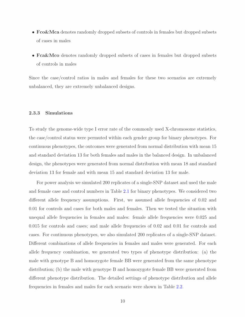
2.3.3 Simulations

To study the genome-wide type I error rate of the commonly used X-chromosome statistics,

the case/control status were permuted within each gender group for binary phenotypes. For

continuous phenotypes, the outcomes were generated from normal distribution with mean 15

and standard deviation 13 for both females and males in the balanced design. In unbalanced

design, the phenotypes were generated from normal distribution with mean 18 and standard

deviation 13 for female and with mean 15 and standard deviation 13 for male.

For power analysis we simulated 200 replicates of a single-SNP dataset and used the male

and female case and control numbers in Table 2.1 for binary phenotypes. We considered two

different allele frequency assumptions. First, we assumed allele frequencies of 0.02 and

0.01 for controls and cases for both males and females. Then we tested the situation with

unequal allele frequencies in females and males: female allele frequencies were 0.025 and

0.015 for controls and cases; and male allele frequencies of 0.02 and 0.01 for controls and

cases. For continuous phenotypes, we also simulated 200 replicates of a single-SNP dataset.

Different combinations of allele frequencies in females and males were generated. For each

allele frequency combination, we generated two types of phenotype distribution: (a) the

male with genotype B and homozygote female BB were generated from the same phenotype

distribution; (b) the male with genotype B and homozygote female BB were generated from

different phenotype distribution. The detailed settings of phenotype distribution and allele

frequencies in females and males for each scenario were shown in Table 2.2.

10

Table 2.2: The genetic models for continuous phenotypes

Scenario

Phenotype distributions ∼ N(µ =Mean, σ = 13) Allele frequency

Mean for male Mean for femaleMale Female

A B AA AB BB

diff-m01f01 15 1615 16 17 0.01 0.01

same-m01f01 15 17

diff-m015f01 15 1615 16 17 0.015 0.01

same-m015f01 15 17

diff-m02f01 15 1615 16 17 0.02 0.01

same-m02f01 15 17

diff-m01f015 15 1615 16 17 0.01 0.015

same-m01f015 15 17

diff-m01f02 15 1615 16 17 0.01 0.02

same-m01f02 15 17

2.4 RESULTS AND CONCLUSIONS

2.4.1 Type I Error Rates

Ozbek et al. (2015) [10] showed the type I error rates of all statistics for common alleles fall

in the Bradleys liberal criterion range of 0.025 to 0.075 [2] in the balanced designs for both

continuous and binary phenotypes. However, the type I error rates of Geno01 were severly

inflated. The type I error rates of all statistics for rare alleles are shown in Table 2.3 and

Table 2.4 for continuous and binary phenotypes respectively.

Table 2.3: Type I error rates for continuous phenotypes

Design Geno01 Sex01 Sex*Geno01 Geno02 Sex02 Sex*Geno02 Clayton.1df Clayton.Sex

Balanced 0.040 0.040 0.066 0.048 0.048 0.066 0.034 0.048

Unbalanced 0.058 0.039 0.040 0.040 0.034 0.040 0.055 0.034

Most results were consistent with those for the common alleles. The one major difference

we found between rare alleles and common alleles is that when the data are unbalanced, the

11

Table 2.4: Type I error rates for binary phenotypes

Design Scenario Geno01 Sex01 Sex*Geno01 Geno02 Sex02

Balanced Bal 0.053 0.056 0.047 0.056 0.059

Balanced Fco&Mco 0.068 0.066 0.043 0.063 0.064

Balanced Fca&Mca 0.058 0.055 0.027 0.056 0.055

Unbalanced Fca 0.064 0.050 0.031 0.055 0.053

Unbalanced Fco 0.055 0.051 0.051 0.051 0.055

Unbalanced Mca 0.098 0.061 0.039 0.074 0.055

Unbalanced Mco 0.074 0.064 0.045 0.051 0.076

Extreme Unbalanced Fco&Mca 0.080 0.050 0.042 0.050 0.061

Extreme Unbalanced Fca&Mco 0.092 0.068 0.042 0.069 0.066

Design Scenario Sex*Geno02 Zheng Clayton.1df Clayton.sex

Balanced Bal 0.047 0.060 0.047 0.040

Balanced Fco&Mco 0.043 0.062 0.075 0.052

Balanced Fca&Mca 0.027 0.063 0.058 0.057

Unbalanced Fca 0.031 0.058 0.035 0.039

Unbalanced Fco 0.051 0.054 0.038 0.036

Unbalanced Mca 0.039 0.059 0.069 0.044

Unbalanced Mco 0.045 0.071 0.093 0.070

Extreme Unbalanced Fco&Mca 0.042 0.056 0.069 0.048

Extreme Unbalanced Fca&Mco 0.042 0.075 0.050 0.045

type I error for Geno01 does not seem to be severely inflated for rare alleles as it was for

the common alleles. To further investigate this phenomenon, we plotted the type I error

rate over different minor allele frequencies in our data and observed that the type I error of

Geno01 is well controlled in the balanced data (Figure 2.1(a)), but it increases with the MAF

in unbalanced datasets (Figure 2.1 (b)) and it increases faster in the extreme unbalanced

datasets (Figure 2.1 (c)).

To understand this phenomenon, we considered the relative frequencies of different geno-

types, and the effect on the models. We illustrate the case of the continuous phenotype in

Figure 2.2: black dots and yellow dots indicate mean value of male phenotype and female

phenotype, respectively. The size of dots is proportional to sample sizes within the cate-

12

0.0 0.1 0.2 0.3 0.4 0.5

0.0

0.2

0.4

0.6

0.8

1.0

Balanced

MAF

Type

I E

rror

(A)

0.0 0.1 0.2 0.3 0.4 0.5

0.0

0.2

0.4

0.6

0.8

1.0

Unbalanced

MAFTy

pe I

Err

or

(B)

0.0 0.1 0.2 0.3 0.4 0.5

0.0

0.2

0.4

0.6

0.8

1.0

Extreme unbalanced

MAF

Type

I E

rror

(C)

Figure 2.1: Type I Error vs. MAF for Geno01 in the (a) balanced design, (b) unbalanced

design, and (c) extreme unbalanced design

gories. Green symbols indicate overall mean value of phenotype. Blue lines indicate fitted

lines that are estimated from the regression model. Under the true null, for the unbalanced

design (assuming the mean of the females is higher than the mean of the males), an arbitrary

positive association is apparently significantly for a common allele (Figure 2.2 (a)). However,

with a rare minor allele, the female homozygous minor allele group has very few or no data

points. The positive association is not significant, thus not affecting the type I error as much

(Figure 2.2 (b))

13

1415

1617

1819

Genotype

Phe

noty

pe

0 1 2

Common Alleles (MAF= 0.494)

458 474

223 433 205

(a)

1415

1617

1819

Genotype

Phe

noty

pe

0 1 2

Rare Alleles (MAF= 0.007)

9176

848 12

(b)

Male Mean Female Mean Overall Mean Fitted line

Figure 2.2: Genetic association for unbalanced design under null hypothesis on the (a)

common allele (b) rare allele

2.4.2 Power

Figure 2.3 shows the results of power analyses for binary phenotypes with allele frequencies

of 0.02 and 0.01 for controls and cases (same in males and females). We observed that the

power of Geno01 is very unstable across different sampling scenarios. In the balanced designs,

Sex01 has relatively higher power. In the unbalanced and extreme unbalanced designs, not

only Sex01 but also Geno02 and Clayton.1df have relatively higher power.

When the allele frequencies for controls and cases are different in males and females, in

which female allele frequencies were 0.025 and 0.015 for controls and cases, and male allele

frequencies of 0.02 and 0.01 for controls and cases, the results are shown on Figure 2.4. The

Clayton’s score-test-based statistic required equal allele frequencies in females and males,

the results for Clayton.1df and Clayton.Sex are not valid. Except the unstable power for

Geno01 that we observed previously and Clayton’s score-test-based statistics, the different

allele frequencies for controls and cases in males and females makes the power of Geno02

14

0.0

0.2

0.4

0.6

0.8

MAF: Fca=0.01 Fco=0.02 Mca=0.01 Mco=0.02

sampling scenarios

Pow

er

Bal Fco&Mco Fca&Mca Fca Fco Mca Mco Fco&Mca Fca&Mco

Geno01Sex01Sex.Geno01Geno02Sex02Sex.Geno02ZhengClayton.1dfClayton.Sex

Figure 2.3: Power analyses on binary phenotype with allele frequencies of 0.02 and 0.01 for

controls and cases (same in males and females)

The label of X-axis denotes sampling scenarios. The first three sampling scenarios are

balanced design. The next four sampling scenarios are unbalanced design. The last two

sampling scenarios are extremely unbalanced designs.

become fluctuated across different sampling scenarios. Sex01 and Sex02 are both stable

across different sampling scenarios and have relatively higher power. These results were

consistent with those for the common alleles.

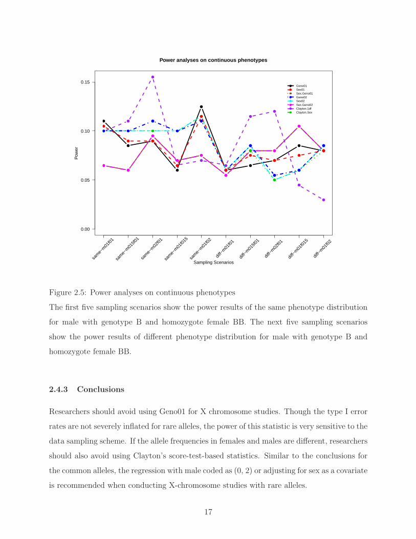
Figure 2.5 shows the results of power analyses for continuous phenotypes. Due to the

assumption of the Clayton’s score-test-based statistic with equal allele frequencies in females

and males, the results for Clayton.1df and Clayton.Sex are only valid when the allele frequen-

cies in females and males are equal. Except for the Clayton.1df and Clayton.Sex, when male

15

0.0

0.2

0.4

0.6

0.8

MAF: Fca=0.015 Fco=0.025 Mca=0.01 Mco=0.02

sampling scenarios

Pow

er

Bal Fco&Mco Fca&Mca Fca Fco Mca Mco Fco&Mca Fca&Mco

Geno01Sex01Sex.Geno01Geno02Sex02Sex.Geno02ZhengClayton.1dfClayton.Sex

Figure 2.4: Power analyses on binary phenotype with different allele frequencies in females

and males, in which female allele frequencies were 0.025 and 0.015 for controls and cases,

and male allele frequencies of 0.02 and 0.01 for controls and cases

The label of X-axis denotes sampling scenarios. The first three sampling scenarios are

balanced design. The next four sampling scenarios are unbalanced design. The last two

sampling scenarios are extremely unbalanced designs.

with genotype B and homozygote female BB were generated from the same phenotype dis-

tribution, Geno02 and Sex02, have relatively higher power. When male with genotype B and

homozygote female BB were generated from different phenotype distribution, Sex.Geno01

and Sex.Geno02 have relatively higher power.

16

0.00

0.05

0.10

0.15

Power analyses on continuous phenotypes

Pow

er

sam

e−m

01f0

1

sam

e−m

015f

01

sam

e−m

02f0

1

sam

e−m

01f0

15

sam

e−m

01f0

2

diff−

m01

f01

diff−

m01

5f01

diff−

m02

f01

diff−

m01

f015

diff−

m01

f02

Sampling Scenarios

Geno01Sex01Sex.Geno01Geno02Sex02Sex.Geno02Clayton.1dfClayton.Sex

Figure 2.5: Power analyses on continuous phenotypes

The first five sampling scenarios show the power results of the same phenotype distribution

for male with genotype B and homozygote female BB. The next five sampling scenarios

show the power results of different phenotype distribution for male with genotype B and

homozygote female BB.

2.4.3 Conclusions

Researchers should avoid using Geno01 for X chromosome studies. Though the type I error

rates are not severely inflated for rare alleles, the power of this statistic is very sensitive to the

data sampling scheme. If the allele frequencies in females and males are different, researchers

should also avoid using Clayton’s score-test-based statistics. Similar to the conclusions for

the common alleles, the regression with male coded as (0, 2) or adjusting for sex as a covariate

is recommended when conducting X-chromosome studies with rare alleles.

17

3.0 STATISTICS FOR DETECTING GENETIC ASSOCIATIONS IN THE

PRESENCE OF ENVIRONMENTAL COVARIATE EFFECT

(SIMULATION STUDY)

3.1 ABSTRACT

In the presence of an environmental covariate effect, there is no consensus on the best strat-

egy to conduct GWAS analysis. In the context of a genome-wide association study, hundreds

of thousands to millions of SNPs are tested, and whichever covariate model we specify is

likely to be imperfect. In addition, the results of the study often focus on the list of SNPs

ordered according to the statistics rather than on certain p-value cutoffs. Therefore, it is

important to investigate the behavior of the extreme values of the statistics rather than

the behavior of the expected values. Gail et al. (2008) discussed this issue and proposed

“detection probability” and “proportion positive” to measure the success of a genomic study

when ranked lists are the primary outcome [5]. In theory, the ranked lists can be dominated

by SNPs with misfit models rather than by true positive results. We conducted a compre-

hensive comparative study to investigate the behavior of different association statistics in

the presence of environmental covariate effect. Selecting the best statistics depends on the

purpose of the study and how a researcher selects disease-associated SNPs. For large studies

that seek for significant signal at a whole genome level should focus on which statistic can

provide the highest power. Exploratory studies that seek for a list of top ranking SNPs

which will be further studied in the future should focus on which statistic can provide the

highest detection probability. Adjusting for the environmental covariate effect or interaction

effect may reduce the power, but it can help with producing more accurate ranked lists.

18

3.2 INTRODUCTION

3.2.1 Common Scenarios Regarding the Environmental Covariate

There have been growing debates over the issue of whether and how to adjust for envi-

ronmental covariates when doing genetic association analysis [9]. Figure 3.1 described the

most common scenarios that discussed in the literature; first, “no covariate effect” the

environmental covariate (E) has no effect, it does not correlate to either phenotype (Y) or

genotype (G), shown in Figure 3.1(a); second, “independent covariate”, the environmen-

tal covariate correlates to phenotype but it is independent of genotype, shown in Figure

3.1(b); “interacting covariate”, the effect of genotype on phenotype depends on this co-

variate (Figure 3.1(c)); and the last, “confounder”, the environmental covariate correlates

to both phenotype and genotype, but it does not mediate their effects (Figure 3.1(d)).

3.2.2 Literature Review

Several studies have investigated the treatment of the environmental covariate in the context

of GWAS analysis. Different, sometimes inconsistent, recommendations were reached by

these studies [12, 8, 20, 21]. It is clear that the environmental covariate should be adjusted

for if it is a confounder, because including the confunder helps control bias and prevent

false discoveries [9]. When the covariate is only correlated to phenotype but not genotype,

including this non-confounding covariate can increase the power to detect genetic association

for both quantitative and binary phenotypes in common disease. However, when the disease

is rare, Pirinen et al. (2012) showed that including non-confounding covariates will reduce

the power in case-control studies [12]. Kuo and Feingold (2010) concluded that the model

without adjusting for covariate is the best model for detecting genetic effects except that

when there is a quite strong interaction between genotype and covariate [8]. Xing and

Xing (2010), however, recommended adjusting for covariates. They argued that adjusting

for covariates may lead to some loss of precision of estimates in logistic regression models,

but it does not always cause loss of power especially when the covariate effect is large [20].

19

Figure 3.1: (a) The environmental covariate (E) has no effect, it does not correlate to both

phenotype (Y) and genotype (G). (b) (E) is an independent covariate. It correlates to Y,

but it is independent of G. (C) E is an interacting covariate, the effect of G on Y depend on

E. (d) E is a confounder. It correlates to both G and Y, but it does not mediate G-Y effects.

Zaitlen et al. (2012) leveraged information from the covariates by modeling the covariates

and phenotypes first, and then evaluating the association between genotypes and model

residuals [21].

3.2.3 Conceptual Framework in Genome-Wide Scan Context

Most of the literature reviewed above focuses on single tests instead of whole genome scans.

The conceptual framework for analyzing whole genome data is different from traditional

statistical analysis. For a single test, we are able to look for the most powerful statistic and

the best fitting model for the data. In the context of GWAS, however, hundreds of thousands

20

to millions of SNPs are tested. Therefore, the model used is likely to be miss-specified for

some genes or even all the genes. The questions of “whether the truly associated genes

will still be ranked near the top” or “whether the top list will be dominated by those genes

which violated the statistical assumptions or by those genes analyzed with the wrong model”

remain unanswered.

3.2.4 Concepts of Detection Probability and Proportion Positive

Most of genome-wide association studies with moderate sample size select disease-associated

SNPs by ranking corresponding statistics instead of using certain p-value thresholds. There-

fore, it is important to investigate the behavior of the extreme values of the statistics rather

than the behavior of the expected values. Gail et al. (2008) proposed the concepts of the

“detection probability (DP)” and “proportion positive (PP)” [5]. DP is defined as the prob-

ability that the test statistic for a specific disease SNP will be among the top T statistic

values in the sample; and PP is defined as the fraction of selected SNPs that are true disease-

associated SNPs. They are related to the “power” and the “type I error” of the statistics

when the top ranked lists are the outcome of the study. Depending on how researchers select

disease-associated SNPs, the statistics with the highest power are not necessarily the same

statistics that provide the most robust ranked lists.


In this chapter, we conduct a comprehensive comparative simulation study to investigate the

behavior of different association statistics in the presence of environmental covariate effects.

We evaluate the traditional power of the statistics as well as which statistics can provide

robust ranked list. We provide guidelines for the choice of statistics and treatment of the

environmental covariate in the whole genome scan context.

21

3.3 STATISTICS AND MATERIALS

3.3.1 Statistics

In this study, we compared four likelihood ratio test based statistics including

1. Phenotype ∼ Genotype compared to the null model, denoted as G.LRT

2. Phenotype ∼ Genotype + Covariate compared to the model with only the Covariate,

denoted as G.E

3. Phenotype ∼ Genotype + Covariate + Genotype × Covariate compared to the model

with Genotype and Covariate, denoted as GE


with only the Covariate, denoted as G.GE [7]

Four chi-square test based statistics and three compound statistics that defined in Kuo and

Feingold (2010) [8] were also compared. The four chi-square test based statistics include

1. χ2 test of independence on the genotype-based table (Table 3.1(a)), denoted asTwoDF23

2. Trend test on the genotype-based table with score vector (0, 1, 2), denoted as Trend23

3. χ2 test of independence on the genotype-based table with 0 vs. 1+2, denoted as Geno22

4. χ2 test of independence on the allele-based table (Table 3.1(b)), denoted as Allele22

The three compound statistics include

1. Minimum p-value among TwoDF23, Trend23, Geno22, and REC, denoted as min4p

2. Minimum p-value among Trend23, Geno22, and REC, denoted as min3p

3. Minimum p-value among TwoDF23 and Geno22, denoted as min2p; where REC is the

trend test on the genotype-based table with score vector (0, 0, 1)

A Case-only statistic was also compared and denoted as CaOnly. The Case-only statistic

uses only the cases and models the relationship between genotype and covariate [11].

The four chi-square test based statistics, three compound statistics and the G.LRT

test for marginal genetic effects. G.E assumes an independent environmental effect (Fig-

ure 3.1(b)) while G.GE assumes an interaction between the genotype and environmental

effect (Figure 3.1(c)). GE and Case-only statistics test for the interaction effects, though in

22

Table 3.1: An illustration for (a) Genotype-based table and (b) Allele-based table

(a) Genotype-based table

AA Aa aa Total

Cases r0 r1 r2 R

Controls s0 s1 s2 S

Total n0 n1 n2 N

(b) Allele-based table

A a Total

Cases 2r0 + r1 2r2 + r1 2R

Controls 2s0 + s1 2s2 + s1 2S

Total 2n0 + n1 2n2 + n1 2N

practice, people use these two tests to detect genetic effects. Although it is hard to antici-

pate which statistics will have the highest power or detection probability, we anticipate that

the statistics that assumes the correct model would perform well. For example, we would

expect that the G.E statistic will be most powerful for the scenario that reflects the situa-

tion presented in Figure 3.1(b) while the G.GE would have the highest power for scenario

presented in Figure 3.1(c). We also anticipate that the GE and Case-only statistics may not

perform as well as the other statistics because they test for only the interaction effects. We

also suspect that the results of the comparison of power and of the comparison of the DP

will be different, since the perspectives of these two types of analyses are different.

3.3.2 Materials

We used the genotype data of chromosome 1 to 22 from the Gene Environment Associa-

tion Studies (GENEVA) pre-term birth dataset (http://www.ncbi.nlm.nih.gov/gap). In this

GWAS dataset, there are approximately 2000 mother-baby pairs genotyped using the Illu-

mina Human 660W-Quad chip. We dropped the mothers’ data and used only 1,795 babies

23

in our study. There are 844 cases (393 female babies and 451 male babies) and 951 con-

trols (470 female babies and 481 male babies) in the dataset. PLINK was used to obtain

the minor allele frequencies and the Hardy-Weinberg equilibrium p-values [13]. We filtered

out the SNPs with MAF < 0.02 and HWE p-value < 0.0001, and included the remaining

515,678 SNPs for the analyses. Sex was used as a covariate in this study. We evaluated the

optimality of statistics by having the correct genome-wide type I error rate, maximal power

and the highest detection probability.

3.4 SIMULATION

3.4.1 Type I Error Rate

To evaluate the genome-wide type I error rate of statistics, we permuted the case/control

status for each subject. To investigate how the covariate effect affects the performance

of each statistic for detecting genetic association, we permuted the case/control status for

females and males separately based on the fixed total number of cases and controls and

sampled different proportions of cases and controls in females and males to generate different

covariate effects. Different odds ratios of sex effect were investigated (ORsex =1.09, 4.58

and 33.71).

3.4.2 Generate Genetic effects

To evaluate the performance of statistics, we simulated true disease-associated SNPs by the

simulation procedure described in Wu et al. (2013) [19]. AssumeM out of N SNPs are truly

associated with disease and the disease risk in the source population is modeled by

logit{P (Yj = 1|Xij)} = µ+M∑

i=1

βiXij,

where Yj is the disease status of subject j, Xij is the number of minor alleles of SNP i for

subject j, µ is the intercept in the source population, and βi is the log odds ratio for SNP i.

24

Following Wu’s paper, βi is assumed to follow a three-component normal mixture model,

π0N(0, σ20) + π1N(0, σ2

1) + π2N(0, σ22),

where π0 = 0.6, π1 = 0.91(1− π0), π2 = 0.09(1− π0), σ20 = (0.058/3)2, σ2

1 = (4× 1502η(1−

η))−1, and σ22 = (4×127.1η(1−η))−1. η denotes the MAF of the SNP. It is a proof-of-concept

simulation and not specific to any disease, thus we chose the same empirical parameters as

Wu’s paper. As in Wu’s paper, SNPs with |β| > 0.058 are considered observable disease-

associated SNPs. Denote M0 as the number of observable disease-associated SNPs. We

generate one β at a time until M0 observable disease-associated SNPs reached, where M0 =

100, 200, or500.

3.4.3 Generate Phenotypes Based on Different Assumed Models

We randomly sampled two chromosomes from the controls to generate the genotype of a

new subject j. The risk of disease given genotype and sex of subject j followed the following

disease model,

logit(pj) =M∑

i=1

βiXij + βESexj +M∑

i=1

βGEi XijSexj.

As we discussed in section 3.2.1, there are four most common scenarios regarding the

environmental covariate. Since it is clear that the environmental covariate should be adjusted

if it is a confounder, we focused our simulation on the remaining three scenarios,

(1) no environmental covariate effect (βE = 0 and βGEi = 0)

(2) with environmental covariate effect (βE = 0.7 and βGEi = 0)

(3) with both environmental covariate effect and interaction effect (βE = 0.7 and βGEi follows

a beta distribution with parameter α = 0.1 and β = 3).

The Phenotype for subject j followed a Bernoulli distribution with probability pj. The

above procedures were repeated until 1000 cases and 1000 controls reached. The results vary

by different set of phenotypes generations. To stabilize the results, 100 sets of replicated

phenotypes were generated based on the same set of βi and Xij.

25

3.4.4 Calculation of Power, Detection Probability and Proportion Positive

We calculated Power as the fraction of observable disease-associated SNPs that reach a p-

value less than the genome-wide significance level (3×10−4/5). The genome-wide significance

level was chosen following Wu’s paper, since the same empirical parameters were used for

generating the genetic effects. The Detection Probability is calculated as the fraction of

observable disease-associated SNPs that are in the top T list and the Proportion Positive

is calculated as the fraction of top T selected SNPs that are observable disease-associated

SNPs, where T from 1 to 60. In practice, people will not be able to look for disease-associated

SNPs with a tiny bit of effect sizes, therefore, we use “observable disease-associated SNPs”

instead of “true disease-associated SNPs”.

26


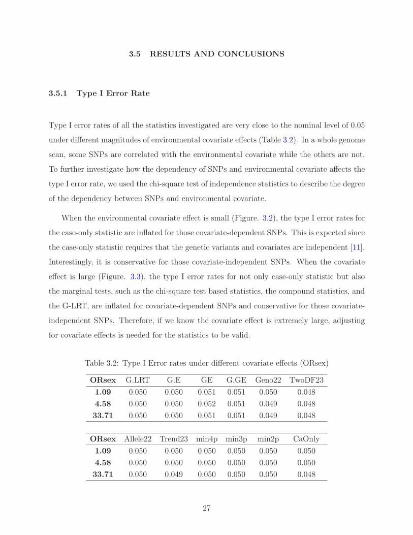
3.5.1 Type I Error Rate

Type I error rates of all the statistics investigated are very close to the nominal level of 0.05

under different magnitudes of environmental covariate effects (Table 3.2). In a whole genome

scan, some SNPs are correlated with the environmental covariate while the others are not.

To further investigate how the dependency of SNPs and environmental covariate affects the

type I error rate, we used the chi-square test of independence statistics to describe the degree

of the dependency between SNPs and environmental covariate.

When the environmental covariate effect is small (Figure. 3.2), the type I error rates for

the case-only statistic are inflated for those covariate-dependent SNPs. This is expected since

the case-only statistic requires that the genetic variants and covariates are independent [11].

Interestingly, it is conservative for those covariate-independent SNPs. When the covariate

effect is large (Figure. 3.3), the type I error rates for not only case-only statistic but also

the marginal tests, such as the chi-square test based statistics, the compound statistics, and

the G-LRT, are inflated for covariate-dependent SNPs and conservative for those covariate-

independent SNPs. Therefore, if we know the covariate effect is extremely large, adjusting

for covariate effects is needed for the statistics to be valid.

Table 3.2: Type I Error rates under different covariate effects (ORsex)

ORsex G.LRT G.E GE G.GE Geno22 TwoDF23

1.09 0.050 0.050 0.051 0.051 0.050 0.048

4.58 0.050 0.050 0.052 0.051 0.049 0.048

33.71 0.050 0.050 0.051 0.051 0.049 0.048

ORsex Allele22 Trend23 min4p min3p min2p CaOnly

1.09 0.050 0.050 0.050 0.050 0.050 0.050

4.58 0.050 0.050 0.050 0.050 0.050 0.050

33.71 0.050 0.049 0.050 0.050 0.050 0.048

27

0.00

0.05

0.10

0.15

0.20

0.25

0.30

ORsex=1.09Ty

pe I

Err

or R

ate

(0,0

.5]

(0.5

,1]

(1,1

.5]

(1.5

,2]

(2,2

.5]

(2.5

,3]

(3,3

.5]

(3.5

,4]

(4,4

.5]

(4.5

,5]

(5,5

.5]

(5.5

,6]

(6,7

8.2]

1122

08

8755

6

6999

7

5394

4

4256

9

3285

2

2608

3

1998

7

1579

0

1223

594

9574

34

2549

9# of SNPs

χGE2 value

Geno22TwoDF23Allele22Trend23min4pmin3pmin2pG.LRTG.EG.GEGECaOnly

Figure 3.2: Type I error rate v.s. GE dependency for small ORsex

28

0.00

0.05

0.10

0.15

0.20

0.25

0.30

ORsex=33.7Ty

pe I

Err

or R

ate

(0,0

.5]

(0.5

,1]

(1,1

.5]

(1.5

,2]

(2,2

.5]

(2.5

,3]

(3,3

.5]

(3.5

,4]

(4,4

.5]

(4.5

,5]

(5,5

.5]

(5.5

,6]

(6,7

8.2]

1122

08

8755

6

6999

7

5394

4

4256

9

3285

2

2608

3

1998

7

1579

0

1223

594

9574

34

2550

0# of SNPs

χGE2 value

Geno22TwoDF23Allele22Trend23min4pmin3pmin2pG.LRTG.EG.GEGECaOnly

Figure 3.3: Type I error rate v.s. GE dependency for large ORsex

29

3.5.2 Power

When the covariate effect is extremely large, we should adjust for covariate effects. Here

we aimed to compare different statistics under various scenarios, where there might exist

moderate environmental covariate effect. After taking average over 100 sets of replicated

datasets, we ranked the power for different association statistics. The exact power is data

dependent and varies significantly from dataset to dataset. The ranking of these statistics

based on the power for each dataset, however, is quite stable. The ranking of power of the

statistics for each simulation scenario were provided in Table 3.3. Three compound statistics

are excluded here, because the p-value for the statistics require dedicated permutation scheme

and the comparison of them is not the main purpose of our study.

Table 3.3: The ranking of power of the statistics for different simulation scenarios include

(1) no environmental covariate effect; (2) with environmental covariate effect; (3) with both

environmental covariate effect and interaction effect

Geno22 TwoDF23 Allele22 Trend23 G.LRT G.E G.GE GE CaOnly

Scenarios 1: βE = 0 and βGEi = 0

M0 = 100 5 7 3 4 1 2 6 9 8

M0 = 200 5 7 4 3 1 1 6 8 9

M0 = 500 5 7 3 4 1 2 6 8 9

Scenarios 2: βE = 0.7 and βGEi = 0

M0 = 100 5 7 3 3 2 1 6 9 8

M0 = 200 5 7 4 3 2 1 6 8 9

M0 = 500 5 7 3 4 1 2 6 8 9

Scenarios 3: βE = 0.7 and βGEi ∼ beta(α = 0.1, β = 3)

M0 = 100 5 7 3 4 1 2 6 9 8

M0 = 200 5 7 2 4 1 3 6 9 8

M0 = 500 5 7 2 3 1 4 6 8 9

As we expected, GE and CaOnly always have the lowest power for all three scenarios,

(1) no environmental covariate effect; (2) with environmental covariate effect; (3) with both

30

environmental covariate effect and interaction effect. G.LRT and G.E, Allele22 and Trend23

have relatively higher power for all three scenarios. More specifically, G.LRT has the highest

power when there is no environmental covariate effect and G.E has the highest power when

there is environmental covariate effect, because they both modeled the underlying true mod-

els. We observed that G.LRT still has the highest power when there are both environmental

covariate effect and interaction effect. Although G.GE modeled the underlying true models,

the extra degree of freedom might cause loss of power. This is consistent with the results

reported by Kuo and Feingold (2010) [8]. The number of observable disease-associated SNPs,

M0, does not affect the ranking of the statistics significantly.

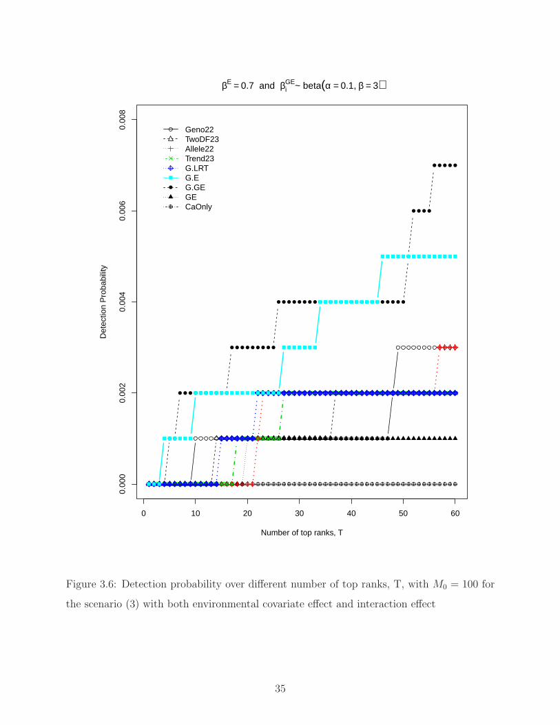
3.5.3 Detection Probability and Proportion Positive

To compare the statistics on their abilities to produce a “robust” top list, we followed Gail

et al.’s strategy and calculated the detection probability and proportion positive of the

statistics. After taking average over 100 sets of replicated datasets, we plotted the detection

probability and proportion positive over different number of top ranks, T . Figure 3.4, Figure

3.5, and Figure 3.6 showed the detection probability over different number of top ranks,

T, with M0 = 100 for the three scenarios, (1) no environmental covariate effect; (2) with

environmental covariate effect; (3) with both environmental covariate effect and interaction

effect, respectively. Consistent with Gail et al. (2008), detection probabilities are pretty

small for realistic assumption of genetic effects (DP <0.01 at T = 100 for genetic effects

β = log(1.1)), due to the large total number of SNPs (515,678 SNPs) and relatively small

number of subjects (1000 cases and 1000 controls). Detection probabilities increase as T

increases. For better visualization, we colored the four higher power statistics (G.LRT, G.E,

Allele22 and Trend23). Except the four higher power statistics, we observed that G.GE also

performs very well in terms of detection probability. The extra degree of freedom might

cause loss of power for G.GE; however, it affects all of the SNPs. Therefore, the ranks of

SNPs are not affected by that and still provide robust detection probability.

Figure 3.7, Figure 3.8, and Figure 3.9 showed the proportion positive over different

number of top ranks, T, while M0 = 100 for the three scenarios, (1) no environmental co-

31

variate effect; (2) with environmental covariate effect; (3) with both environmental covariate

effect and interaction effect, respectively. Again, due to large number of SNPs and small

number of subjects, the proportion positives are small as well. When the number of top

ranks, T, is too small, it is hard to discover true disease-associated SNPs. However, when

the number of top ranks, T, is increasing, it will introduce false positives so that the pro-

portion positives decrease with increasing number of T. Therefore, the selection of T is also

critical for researchers when providing a top list of disease-associated SNPs as study results.

As what we discovered in the detection probability, except the four higher power statistics,

G.GE also perform very well in terms of proportion positives.

However, these results are based on one set of random generated βi and Xij . Multiple

sets of random generated βi and Xij should be done in the future to provide more general

and convincing results.

3.5.4 Conclusions

Our simulation studies indicate that the relative performance of different statistics in the

presence of environmental covariate effects differs depending on whether we evaluate their

performance by simple power or detection probability. Thus, selecting the best statistics

depends on the purpose of the study and how a researcher selects disease-associated SNPs.

For large studies that seek for significant signal at a whole genome level should focus on which

statistic can provide the highest power. In our results, G.LRT, G.E, Allele22 and Trend23

have relatively higher power for all different underlying models. Exploratory studies that

seek for a list of top ranking SNPs which will be further studied in the future should focus on

which statistic can provide the highest detection probability. Our simulations indicate that

although the top performing statistics overlap largely between these two types of approach

(power and DP), there are some differences. The G.GE model does not seem to be the best

choice to optimize the power of the analysis due to the fact that an extra degree of freedom

is used. However, when ranking the SNPs by their values of the statistics, this no longer

matters. Even when there is no interaction between the genetic and environmental effect,

the ranking of the SNPs should not be affected.

32

0 10 20 30 40 50 60

0.00

00.

001

0.00

20.

003

0.00

40.

005

βE = 0 and βiGE = 0

Det

ectio

n P

roba

bilit

y

Number of top ranks, T

Geno22TwoDF23Allele22Trend23G.LRTG.EG.GEGECaOnly

Figure 3.4: Detection probability over different number of top ranks, T, with M0 = 100 for

the scenario (1) no environmental covariate effect

33

0 10 20 30 40 50 60

0.00

00.

001

0.00

20.

003

0.00

4

βE = 0.7 and βiGE = 0

Det

ectio

n P

roba

bilit

y




the scenario (2) with environmental covariate effect

34

0 10 20 30 40 50 60

0.00

00.

002

0.00

40.

006

0.00

8

βE = 0.7 and βiGE~ beta(α = 0.1, β = 3)

Det

ectio

n P

roba

bilit

y




the scenario (3) with both environmental covariate effect and interaction effect

35

0 10 20 30 40 50 60

0.00

00.

005

0.01

00.

015

0.02

00.

025

0.03

0


Pro

port

ion

Pos

itive



Figure 3.7: Proportion positive over different number of top ranks, T, with M0 = 100 for

the scenario (1) no environmental covariate effect

36

0 10 20 30 40 50 60

0.00

00.

005

0.01

00.

015

0.02

00.

025

0.03

0


Pro

port

ion

Pos

itive




the scenario (2) with environmental covariate effect

37

0 10 20 30 40 50 60

0.00

00.

005

0.01

00.

015

0.02

00.

025

0.03

0


Pro

port

ion

Pos

itive




the scenario (3) with both environmental covariate effect and interaction effect

38

4.0 ANALYTIC CALCULATION OF DETECTION PROBABILITY AND

PROPORTION POSITIVE IN THE COVARIATE MODEL

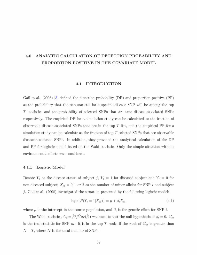
4.1 INTRODUCTION

Gail et al. (2008) [5] defined the detection probability (DP) and proportion positive (PP)

as the probability that the test statistic for a specific disease SNP will be among the top

T statistics and the probability of selected SNPs that are true disease-associated SNPs

respectively. The empirical DP for a simulation study can be calculated as the fraction of

observable disease-associated SNPs that are in the top T list, and the empirical PP for a

simulation study can be calculate as the fraction of top T selected SNPs that are observable

disease-associated SNPs. In addition, they provided the analytical calculation of the DP

and PP for logistic model based on the Wald statistic. Only the simple situation without

environmental effects was considered.

4.1.1 Logistic Model

Denote Yj as the disease status of subject j, Yj = 1 for diseased subject and Yj = 0 for

non-diseased subject; Xij = 0, 1 or 2 as the number of minor alleles for SNP i and subject

j. Gail et al. (2008) investigated the situation presented by the following logistic model:

logit{P (Yj = 1|Xij)} = µ+ βiXij, (4.1)

where µ is the intercept in the source population, and βi is the genetic effect for SNP i.

The Wald statistics, Ci = β2i /V ar(βi) was used to test the null hypothesis of βi = 0. Cm

is the test statistic for SNP m. It is in the top T ranks if the rank of Cm is greater than

N − T , where N is the total number of SNPs.

39

4.1.2 Analytic calculation of detection probability

Assume that the first M out of N SNPs are disease-associated SNPs. Let Gi be the distri-

bution of Ci and gi(c) be the density of Ci for i = 1, 2, . . . ,M . Consider a particular disease

SNP, namely SNP 1. Given c and a small interval dc, Gail et al. (2008) defined H1(c) be the

event that C1 is in the interval [c, c+dc), and H2(m; c,M) be the event that m of the remain-

ing M − 1 disease-associated SNPs have Ci values greater than c, and H3(T −m− 1; c,m)

be the event that no more than T −m− 1 non-disease SNPs have Ci values greater than c.

The intersection of these three events implies that C1 is in the top T ranks.

Conditional on the allele frequency and genetic effect, DP for SNP 1 (denote as DP1)

then is given by

DP1 =

∫

∞

0

min(M−1,T−1)∑

m=0

P (H2(m; c)|c)T−1−m∑

s=0

(

N −M

s

)

{1− F (c)}s{F (c)}N−M−s

g1(c)dc,

(4.2)

where F is the central chi-square distribution with 1 degree of freedom. P (H2(m; c)|c) needs

to be calculated recursively.

If disease SNPs have the same distribution, G(c), then (4.2) can be simplifies to

DP =

∫

∞

0

min(M−1,T−1)∑

m=0

(

M − 1

m

)

g(c){1−G(c)}m{G(c)}M−1−m

×

T−1−m∑

s=0

(

N −M

s

)

{1− F (c)}s{F (c)}N−M−s

]

dc. (4.3)

where G is a non-central chi-square distribution with 1 degree of freedom. For a fixed genetic

effect model with fixed allele frequencies, the non-centrality parameter for the Wald test is

β2/V ar(β).

40

4.1.3 Analytic calculation of proportion positive

PP is the fraction of selected SNPs that are true disease-associated SNPs. Once DP is

calculated, PP can be calculated by the following formula,

PP = (M/T )(DP ) (4.4)


Gail et al. (2008) analytically defined DP and PP based on Wald statistics. They also stud-

ied the factors that affect the performance of DP and PP such as the magnitude of genetic

effect, the number of non-disease SNPs, and number of selected SNPs. However, their works

were under a simple logistic model without considering an environmental covariate effect.

We further extended Gail et al.’s calculation to incorporate the environmental covariate ef-

fect and compare the analytical DP of the four likelihood ratio test based statistics that

were defined in chapter 3 (G.LRT, G.E, GE, G.GE) for the three scenarios, (1) no environ-

mental covariate effect; (2) with environmental covariate effect; (3) with both environmental

covariate effect and interaction effect.

4.2 ANALYTICAL CALCULATION OF DETECTION PROBABILITY

AND PROPORTION POSITIVE IN THE COVARIATE MODEL

To extend DP calculations presented in (4.2) and (4.3) to situations when the environmental

covariate effect exists, the non-centrality parameter for the distribution of disease-associated

SNPs, G, and the degree of freedom needs to be derived for each model investigated.

Self et al. (1992) [15] proposed an approach of non-central chi-square approximation to

the distribution of the likelihood ratio statistic within the framework of generalized linear

models. Shieh (2000) [16] simplified the calculation of non-centrality parameter and showed

41

that under alternative hypothesis the non-centrality parameter for a likelihood ratio statistic

can be calculated as

nEXZ

[

2

{

eθ

1 + eθ[θ − θ0]− log

[

1 + eθ

1 + eθ0

]}]

, (4.5)

where n denotes total number of subjects, X denotes genotypes, Z denotes the covariate. θ

and θ0 denote the canonical parameter values evaluated at the alternative and null models,

respectively. For example, ψ and λ are the estimated regression coefficient that evaluated at

the alternative model; ψ0 and λ0 are the estimated regression coefficient that evaluated at

the null model. The estimated non-centrality parameter (4.5) can be calculated as

n∑

X

∑

Z

[

2

{

eXψ+Zλ

1 + eXψ+Zλ[(Xψ +Zλ)− (Xψ0 +Zλ0)]− log

[

1 + eXψ+Zλ

1 + eXψ0+Zλ0

]}

f(X,Z)

]

,

(4.6)

where f(X,Z) denotes the emperical join distribution of genotype and covariate. Detailed

derivations of (4.5) are included in Appendix A.

4.3 STATISTICS AND MATERIALS

4.3.1 Statistics

In this study, we focus on comparing the analytical DPs of the following four likelihood ratio

test based statistics

1. Phenotype ∼ Genotype compared to the null model, denoted as G.LRT

2. Phenotype ∼ Genotype + Covariate compared to the model with only covariate, denoted

as G.E

42


with genotype and covariate, denoted as GE;


with only covariate, denoted as G.GE [7]

4.3.2 Materials

Data with a total of 1000 cases and 1000 controls were generated as what we described in

section 3.4. M0 = 100 out of 515,678 SNPs were observable disease-associated SNPs. The

genetic effects βi were generated from a three-component normal mixture model. The risk

of disease given genotype and sex of subject j followed the following disease model,

logit(pj) =M∑

i=1

βiXij + βESexj +M∑

i=1

βGEi XijSexj.

Phenotype for subject j followed a Bernoulli distribution with probability pj. The results

vary by different set of phenotypes generations. Ten sets of replicated phenotypes were

generated to stabilize the results. The analytical detection probabilities were calculated for

each observable disease-associated SNPs based on their MAF and genetic effects βi then

average over 100 SNPs and 10 replicated phenotypes.

The three scenarios that considered in this chapter are the same as in Chapter 3,

(1) no environmental covariate effect (βE = 0 and βGEi = 0)

(2) with environmental covariate effect (βE = 0.7 and βGEi = 0)

(3) with both environmental covariate effect and interaction effect (βE = 0.7 and βGEi follows

a beta distribution with parameter α = 0.1 and β = 3).

43


4.4.1 Results

Figure. 4.1, Figure. 4.2, and Figure. 4.3 showed the results of analytical DPs over

different number of top ranks, T, for the three scenarios, (1) no environmental covariate

effect; (2) with environmental covariate effect; (3) with both environmental covariate effect

and interaction effect, respectively. The analytical DPs are small due to the large total

number of SNPs (515,678 SNPs) and relatively small number of subjects (1000 cases and

1000 controls). The analytical DPs increase with increasing T while analytical PPs decrease

as T increases (results for analytical PPs are shown in Appendix B).

The results are similar to what was observed when using empirical calculation of DP and

PP (Chapter 3). For better visualization, we plotted the empirical DPs from section 3.5.3

with corresponding color in Figure. 4.4, Figure. 4.5, and Figure. 4.6. The analytical DPs

for G.LRT, G.E, and G.GE are very close for the first two scenarios. For the third scenario,

when there are both environmental covariate effect and interaction effect, G.E, and G.GE

perform better than G.LRT. Thus, it is important to adjust for environmental covariate

effect, especially when there is an interaction between the genetic and environmental effects.

GE has the worst analytical detection probabilities for all three scenarios as expected, given

that it only detects the interaction effect.

4.4.2 Conclusions

The analytical DPs and PPs are similar to the results for the empirical DPs and PPs. G.E

and G.GE have the highest analytical DPs and PPs for all three scenarios. The analytical

DPs and PPs for G.LRT are close to G.E and G.GE except in the case where there are both

environmental covariate effect and interaction effect. Given the above observation, to opti-

mize DP and PP, we should always adjust for environmental covariate effect in the analysis.

These results are based on one set of random generated βi and Xij . Multiple sets of random

generated βi and Xij should be done in the future to provide more general and convincing

results.

44

0 10 20 30 40 50 60

0.00

0.01

0.02

0.03

0.04

0.05



Det

ectio

n P

roba

bilit

y

G.LRTG.EG.GEGE

Figure 4.1: Analytical detection probability over different number of top ranks, T, for the

scenario (1) no environmental covariate effect

45

0 10 20 30 40 50 60

0.00

0.01

0.02

0.03

0.04

0.05

0.06



Det

ectio

n P

roba

bilit

y

G.LRTG.EG.GEGE


scenario (2) with environmental covariate effect

46

0 10 20 30 40 50 60

0.00

0.01

0.02

0.03

0.04

0.05



Det

ectio

n P

roba

bilit

y

G.LRTG.EG.GEGE


scenario (3) with both environmental covariate effect and interaction effect

47

0 10 20 30 40 50 60

0.00

00.

001

0.00

20.

003

0.00

40.

005


Det

ectio

n P

roba

bilit

y


G.LRTG.EG.GEGE

Figure 4.4: Empirical detection probability over different number of top ranks, T, for the


48

0 10 20 30 40 50 60

0.00

00.

001

0.00

20.

003

0.00

4


Det

ectio

n P

roba

bilit

y


G.LRTG.EG.GEGE



49

0 10 20 30 40 50 60

0.00

00.

002

0.00

40.

006

0.00

8


Det

ectio

n P

roba

bilit

y


G.LRTG.EG.GEGE



50

5.0 DISCUSSION AND FUTURE WORK

5.1 DISCUSSION

The analysis of the X-chromosome data is more complicated than the analysis of autosomal

chromosome data due to the fact that males have only one copy of the X-chromosome

while the females have two. Previous investigations of X-chromosome statistics focused on

common allele SNPs. In this dissertation, I studied the behavior of different X-chromosome

association statistics with rare alleles. The conclusions were mostly consistent with those

for the common alleles with the exception that the type I error for the logistic regression

with male coded as (0, 1) increases with the minor allele frequency for certain data sampling

schemes. Overall we conclude that male genotypes should be coded as (0, 2) or consider

adding sex as a covariate when conducting X chromosome studies.

In a conventional single-test context one looks for the most powerful statistic and the

best fitted model for the data. However, there is no single statistic or model that perfectly

fit for all of hundreds of thousands of SNPs in a whole genome scans. Previous works on the

comparison of different statistics have been focused on the situation without environmental

effects. In this dissertation, I investigated the behavior of different association statistics in

the presence of environmental covariate effects.

Selecting the best statistics depends on the purpose of the study and how a researcher

selects disease-associated SNPs. If the disease-associated SNPs are defined by a pre-set

p-value, then G.LRT, G.E, Allele22 and Trend23 with relatively higher power are recom-

mended. For exploratory studies that seek for a list of top ranking genes, then not only

G.LRT, G.E, Allele22 and Trend23, but also G.GE with higher detection probabilities are

recommended.

51

It is worth mentioning that GE and CaOnly are mainly testing for the gene-environment

interaction. Although occasionally used in practice, they are not a good choice to test for

genetic effects. Our simulation results also demonstrated that these two statistics perform

more poorly than all the other statistics investigated in this study. In addition, the case-

only statistics utilized only the cases and modeled the relationship between genotype and

covariate. Therefore, in term of sample size, it is not a fair comparison for the case-only

statistics.

5.2 FUTURE WORK

• Gail et al. (2008) studied the analytical DPs and PPs using a fixed genetic effect model

with fixed allele frequencies. We extended this idea to more flexible and realistic situa-

tions with various genetic effects and allele frequencies, as well as gene by environment

interaction. However, our results are still based on a limited set of randomly generated

genetic effects and genotypes. Multiple sets of randomly generated data should be used

to provide more general and convincing results.

• We evaluated the statistics for the scenarios with binary outcome and one binary envi-

ronmental covariate. The behavior of the statistics under the quantitative outcome with

a quantitative environmental covariate or even with multiple environmental covariates is

still unstudied.

• The analytical DPs and PPs calculations can be extended to the Chi-square test based

statistics that we discussed in section 3.3.

52

APPENDIX A

THE NON-CENTRALITY OF THE NON-CENTRAL CHI-SQUARE

DISTRIBUTION FOR THE LIKELIHOOD RATIO STATISTICS

Generalized linear models assume the independent response variables Yi, i = 1, . . . , n has a

probability distribution belongs to the exponential family with the form:

f(Yi) = exp

{

Y θ − b(θ)

a(φ)+ c(Y, φ)

}

The expected value of Y , E(Y ) = µ is related to the canonical parameter θ, by the equation

µ = b′(θ), where b′ is the first derivative of b. The scale parameter φ is assumed known. The

link function g links the linear predictors (η) and the mean response (µ) via the expression

η = g(µ). The linear predictors, η, can be written as XTψ + Z

Tλ, where X and Z are

p-vector and q-vector of covariates, and ψ and λ are unknown regression coefficients.

The likelihood ratio test statistics for testing the hypothesis H0 : ψ = ψ0 (λ is treated as

nuisance parameter) is given by

2[ℓ(ψ, λ)− ℓ(ψ0, λ0)]

where ℓ(ψ, λ) denotes the log-likelihood function. (ψ, λ) and (ψ0, λ0) are the maximum

53

likelihood estimators of (ψ, λ) under the alternative and null models, respectively. The

likelihood ratio test statistic under null hypothesis follows a central chi-square distribution

with p degrees of freedom; while under the alternative hypothesis, the likelihood ratio test

statistic follows a non-central chi-square distribution with p degrees of freedom. The non-

centrality parameter is calculating by equating the expected value of a non-central chi-square

random variable to an approximation of the expected value of the likelihood ratio statistic.

In Self et al. (1992) [15], the likelihood ratio statistic is decomposed into three terms,

2[ℓ(ψ, λ)− ℓ(ψ0, λ0)] = 2[ℓ(ψ, λ)− ℓ(ψ, λ)]

− 2[ℓ(ψ0, λ0)− ℓ(ψ0, λ∗

0)]

+ 2[ℓ(ψ, λ)− ℓ(ψ0, λ∗

0)] (A.1)

where λ∗0 is the limiting value of λ0 as described in Self and Mauritsen (1988) [14].

According to Cordeiro (1983) [4], the expected value of the first term in (A.1) is

E{2[ℓ(ψ, λ)− ℓ(ψ, λ)]} ≈ p+ q. (A.2)

By Self et al. (1992) [15] and references cited therein, the expected value of the second term

in (A.1) is

E{2[ℓ(ψ0, λ0)− ℓ(ψ0, λ∗

0)]} ≈ q. (A.3)

The third term in (A.1) does not involve any maximum likelihood estimators of (ψ, λ). Based

on Shieh (2000) [16], its expectation can be written as

n∆ = nEZX [2a−1(φ){b′(θ)[θ − θ0]− [b(θ)− b(θ0)]}]. (A.4)

54

For Bernouli outcomes in our case, a(φ) = 1 and b′(θ) = eθ/(1 + eθ), n∆ can be further

calculated as

nEXZ

[

2

{

eθ

1 + eθ[θ − θ0]− log

[

1 + eθ

1 + eθ0

]}]

.

The expected value of a non-central chi-square random variable with p degrees of freedom

and non-centrality parameter γ is p+ γ. Equating this to the approximations (A.2), (A.3),

and (A.4), the expected value of likelihood ratio statistics is (p+ q)− q + n∆∗, which leads

to the non-centrality parameter γ = n∆∗

55

APPENDIX B

RESULTS FOR ANALYTICAL PROPORTION POSITIVE OVER

DIFFERENT NUMBER OF TOP RANKS

56

0 10 20 30 40 50 60

0.00

00.

002

0.00

40.

006

0.00

80.

010

0.01

2



Pro

port

ion

Pos

itive

G.LRTG.EG.GEGE

Figure B1: Analytical proportion positive over different number of top ranks, T, for the


57

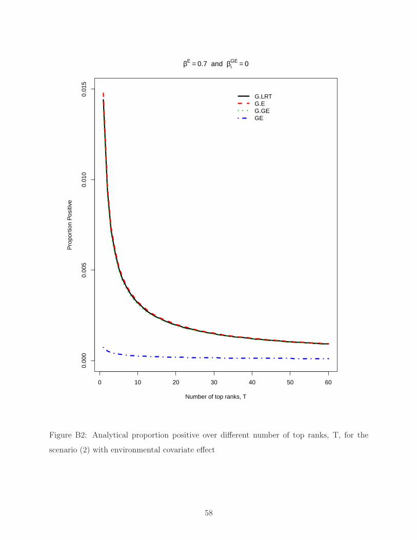
0 10 20 30 40 50 60

0.00

00.

005

0.01

00.

015



Pro

port

ion

Pos

itive

G.LRTG.EG.GEGE



58

0 10 20 30 40 50 60

0.00

00.

002

0.00

40.

006

0.00

80.

010

0.01

2



Pro

port

ion

Pos

itive

G.LRTG.EG.GEGE



59

BIBLIOGRAPHY

[1] C. E. Bonferroni. Teoria statistica delle classi e calcolo delle probabilita. Libreria inter-nazionale Seeber, 1936.

[2] J. V. Bradley. Robustness? British Journal of Mathematical and Statistical Psychology,31(2):144–152, 1978.

[3] D. Clayton. Testing for association on the x chromosome. Biostatistics, 9(4):593–600,2008.

[4] G. M. Cordeiro. Improved likelihood ratio statistics for generalized linear models. Jour-nal of the Royal Statistical Society. Series B (Methodological), pages 404–413, 1983.

[5] M. H. Gail, R. M. Pfeiffer, W. Wheeler, and D. Pee. Probability of detecting disease-associated single nucleotide polymorphisms in case-control genome-wide associationstudies. Biostatistics, 9(2):201–215, 2008.

[6] E. Gubb and R. Matthiesen. Introduction to omics. In Bioinformatics Methods inClinical Research, pages 1–23. Springer, 2010.

[7] P. Kraft, Y.-C. Yen, D. O. Stram, J. Morrison, and W. J. Gauderman. Exploiting gene-environment interaction to detect genetic associations. Human heredity, 63(2):111–119,2007.

[8] C.-L. Kuo and E. Feingold. What’s the best statistic for a simple test of genetic asso-ciation in a case-control study? Genetic epidemiology, 34(3):246–253, 2010.

[9] J. Mefford and J. S. Witte. The covariate’s dilemma. PLoS genetics, 8(11):e1003096,2012.

[10] U. Ozbek, H.-M. Lin, Y. Lin, D. E. Weeks, W. Chen, J. Shaffer, S. M. Purcell, andE. Feingold. Statistics for x-chromosome associations. submitted to xxx, 2015.

[11] W. W. Piegorsch, C. R. Weinberg, and J. A. Taylor. Non-hierarchical logistic models andcase-only designs for assessing susceptibility in population-based case-control studies.Statistics in medicine, 13(2):153–162, 1994.

60

[12] M. Pirinen, P. Donnelly, and C. C. Spencer. Including known covariates can reducepower to detect genetic effects in case-control studies. Nature genetics, 44(8):848–851,2012.

[13] S. Purcell, B. Neale, K. Todd-Brown, L. Thomas, M. A. Ferreira, D. Bender, J. Maller,P. Sklar, P. de Bakker, M. Daly, and S. Pak. Plink: a tool set for whole-genomeassociation and population-based linkage analyses. The American Journal of HumanGenetics, 81(3):559–575, 2007.

[14] S. G. Self and R. H. Mauritsen. Power/sample size calculations for generalized linearmodels. Biometrics, pages 79–86, 1988.

[15] S. G. Self, R. H. Mauritsen, and J. Ohara. Power calculations for likelihood ratio testsin generalized linear models. Biometrics, pages 31–39, 1992.

[16] G. Shieh. On power and sample size calculations for likelihood ratio tests in generalizedlinear models. Biometrics, 56(4):1192–1196, 2000.

[17] J. D. Storey. A direct approach to false discovery rates. Journal of the Royal StatisticalSociety: Series B (Statistical Methodology), 64(3):479–498, 2002.

[18] A. L. Wise, L. Gyi, and T. A. Manolio. exclusion: toward integrating the x chromo-some in genome-wide association analyses. The American Journal of Human Genetics,92(5):643–647, 2013.

[19] J. Wu, R. M. Pfeiffer, and M. H. Gail. Strategies for developing prediction models fromgenome-wide association studies. Genetic epidemiology, 37(8):768–777, 2013.

[20] G. Xing and C. Xing. Adjusting for covariates in logistic regression models. Geneticepidemiology, 34(7):769, 2010.

[21] N. Zaitlen, S. Lindstrom, B. Pasaniuc, M. Cornelis, G. Genovese, S. Pollack, A. Barton,H. Bickeboller, D. W. Bowden, S. Eyre, et al. Informed conditioning on clinical covariatesincreases power in case-control association studies. PLoS genetics, 8(11):e1003032, 2012.

[22] D. V. Zaykin and L. A. Zhivotovsky. Ranks of genuine associations in whole-genomescans. Genetics, 171(2):813–823, 2005.

[23] G. Zheng, J. Joo, C. Zhang, and N. L. Geller. Testing association for markers on the xchromosome. Genetic epidemiology, 31(8):834–843, 2007.

61

behavior of statistics for genetic association in a …

Documents