behavioral biases of investment advisors -...
TRANSCRIPT
BEHAVIORAL BIASES OFINVESTMENT ADVISORS - The Effectof Overconfidence and HindsightBias
Finance
Master's thesis
Antti Seppälä
2009
Department of Accounting and Finance
HELSINGIN KAUPPAKORKEAKOULUHELSINKI SCHOOL OF ECONOMICS
Helsinki School of Economics Abstract Master’s Thesis August 31, 2009 Antti Seppälä
BEHAVIORAL BIASES OF INVESTMENT ADVISORS: THE EFFECT OF OVERCONFIDENCE AND HINDSIGHT BIAS
PURPOSE OF THE STUDY
The objective of this thesis is to examine the effects of three behavioral biases on investment
advisors. These biases are hindsight bias, overconfidence and self-attribution bias. A survey study is
carried out to find out how the studied biases affect the investment advisors. The same survey study is
also carried out for two control groups for comparative purposes. In addition, the effects of individual
thinking style and cognitive abilities on the exposure to behavioral biases are studied.
DATA
The data in this study is collected in controlled field surveys. The surveys are carried for three
separate groups of people; financial professionals, university students and employees of an
engineering company The participants of the surveys answer a questionnaire that contains financial
market related estimation tasks.
The main insight of the survey study is the two-pronged structure of the surveys. The ability to
recollect answers and repeat the surveys enables the examination of the biases at issue. The biases
are studied by comparing observations from different phases of the surveys to each other. Hindsight
bias is observed by differences between initial answers and the recollections. Overconfidence is
studied using initial answers and realized results. Analyses of self-attribution bias use initial answers
from first and second round.
RESULTS
The main finding of this study is that people in general are exposed to the studied behavioral biases
but the degree and impact are affected by experience and other characteristics. Investment advisors
are generally less exposed to hindsight bias than other people. Moreover, professionals generally
outperform other people with lower level of confidence, which indicates lower overconfidence.
However, professionals are most exposed to self-attribution bias. The results indicate that in
addition to expertise, individual thinking style explains behavioral biases. People with high faith
in intuition are more exposed to behavioral biases. Overall, the results of this thesis provide
valuable new information on behavioral biases and investment advisors.
KEYW ORDS
Behavioral Finance, Investment advisors, overconfidence, hindsight bias, self-attribution bias

Table of Contents
1. INTRODUCTION ...................................................................................................................................................... 3
1.2. BACKGROUND AND MOTIVATION ...................................................................................................................... 3
1.3. RESEARCH QUESTIONS ....................................................................................................................................... 4
1.4. CONTRIBUTION ................................................................................................................................................... 6
1.5. RESULTS SUMMARY ............................................................................................................................................ 6
1.6. STRUCTURE OF THE STUDY ................................................................................................................................ 7
2. PSYCHOLOGICAL FACTORS IN DECISION MAKING ............................................................................... 8
2.1. HINDSIGHT BIAS .................................................................................................................................................. 9
2.2. OVERCONFIDENCE ............................................................................................................................................11
2.3. SELF-ATTRIBUTION BIAS...................................................................................................................................11
2.4. FACTORS AFFECTING EXPOSURE TO BEHAVIORAL BIASES ..............................................................................12
3. DATA AND METHODS .........................................................................................................................................16
3.1. DATA .................................................................................................................................................................16
3.2. METHODS ..........................................................................................................................................................25
4. RESULTS ..................................................................................................................................................................32
4.1. HINDSIGHT BIAS ................................................................................................................................................32
4.2. OVERCONFIDENCE ............................................................................................................................................54
4.3. SELF-ATTRIBUTION BIAS...................................................................................................................................67
4.4. COGNITIVE-EXPERIENTIAL SELF-THEORY ........................................................................................................70
5. CONCLUSIONS ......................................................................................................................................................73
6. REFERENCES .........................................................................................................................................................76
7. EXHIBITS .................................................................................................................................................................81
7.1. DISTRIBUTIONS OF THINKING STYLE SCORES ..................................................................................................81
7.2. REGRESSION STATISTICS...................................................................................................................................82
7.3. QUESTIONNAIRE SHEETS...................................................................................................................................86
2
LIST OF TABLES
Table 1 – Survey dates and return estimate periods...........................................................................................................17
Table 2 – Distribution of age ...............................................................................................................................................18
Table 3 – Return statistics....................................................................................................................................................23
Table 4 – Hindsight bias, asset selection effect 1/3 ...........................................................................................................34
Table 5 – Hindsight bias, asset selection effect 2/3 ...........................................................................................................37
Table 6 – Hindsight bias – asset selection effect 3/3 .........................................................................................................39
Table 7 – Hindsight bias, sign of return effect 1/2 .............................................................................................................43
Table 8 – Hindsight bias, sign of return effect 2/2 .............................................................................................................46
Table 9 – Hindsight bias, drift of return effect ...................................................................................................................50
Table 10 – Hindsight bias, strength of view effect ............................................................................................................53
Table 11 – Overconfidence, confidence boundaries 1/2....................................................................................................54
Table 12 – Overconfidence, confidence boundaries 1/2....................................................................................................55
Table 13 – Overconfidence, volatility estimation ..............................................................................................................56
Table 14 – Overconfidence, confidence-performance 1/3 ................................................................................................60
Table 15 – Overconfidence, confidence-performance 2/3 ................................................................................................62
Table 16 – Overconfidence, confidence-performance 3/3 ................................................................................................64
Table 17 – overconfidence, confidence ..............................................................................................................................66
Table 18 – Self-attribution bias, individual answers test ...................................................................................................67
Table 19 – Self-attribution bias, person level test ..............................................................................................................69
Table 20 – Individual thinking ............................................................................................................................................71
LIST OF FIGURES
Figure 1 – Distribution of experience .................................................................................................................................19
Figure 2 – Personal investment experience ........................................................................................................................21
Figure 3 – Return development timeline ............................................................................................................................24
Figure 4 – Hindsight bias, asset selection effect ................................................................................................................41
Figure 5 – Hindsight bias, sign of return effect ..................................................................................................................48
Figure 6 – Hindsight bias, drift of return effect .................................................................................................................51
Figure 7 – Overconfidence, volatility estimation ...............................................................................................................59
Figure 8 – overconfidence, confidence-performance 1/2 ..................................................................................................61
Figure 9 – overconfidence, confidence-performance 2/2 ..................................................................................................62
Figure 10 – Self-attribution bias, person level test ............................................................................................................69
Figure 11 – Individual thinking ...........................................................................................................................................72
3
1. Introduction
Investment advisors are professionals who assist their clients in financial decision making issues
such as investing, insurance, borrowing, taxation and retirement planning. Thus investment
advisors have a great impact on their clients’ decisions. The advices and recommendations
investment advisors give to their clients are naturally affected by the beliefs and conceptions they
possess. Biases in these beliefs and conceptions can strongly affect the decision making of the
clients and thus it is important to study investment advisors’ behavioral biases.
1.2. Background and Motivation
Previous literature shows that psychological factors have a substantial effect on people’s
decision making. Tversky and Kahneman (1974) present that people rely on a limited number of
heuristic principles which in general are quite useful, but sometimes lead to severe and systematic
biases. This study focuses to examine three such biases; hindsight bias, overconfidence and self-
attribution bias.
Hindsight bias refers to a tendency to perceive own performance better than it actually is,
after learning the realization. Biais and W eber (2008) find that for hindsight biased agents the ex-
post recollection of the initial belief will be closer to the realization than the true ex-ante
expectation. According to Buksar and Conolly (1988) hindsight bias hinders learning from past
experience. In a similar vein Biais and W eber (2008) present that hindsight biased agents also fail
to remember how ignorant they were before observing outcomes and answers This leads agents
to underestimate volatility, which again results in inefficient portfolio choice and poor risk
management. One explanation of hindsight bias is the availability heuristic: the event that did
occur is more salient in one's mind than the possible outcomes that did not.
Overconfidence refers to the habit of overestimating own ability to perform in given tasks.
People tend to be overconfident about own capabilities and level of knowledge. Overconfidence
has several forms, such as ‘better than average’, ‘optimism bias’ and ‘setting too narrow
confidence limits’. According to Barber and Odean (2000) overconfidence causes excess trading
which can be risky to financial well being.
4
Self-attribution bias refers to a tendency to overestimate the degree to which people are
responsible for their own success. Hastorf, Schneider, and Polifka (1970) write, "W e are prone to
attribute success to our own dispositions and failure to external forces”. In a similar vein, Gervais
and Odean (2001) find that success of traders leads to increased overconfidence. W hen a trader is
successful, he attributes too much of his success to his own ability and revises his beliefs about
his ability upward too much, which increases overconfidence.
However, the exposure to behavioral biases is not homogenous. Certain factors are reported
to explain the level of exposure. Lewellen, Lease and Schlarbaum (1977) find that men have
stronger tendency to overconfident behavior than woman have. Korniotis and Kumar (2007)
show that overconfidence decreases with age. Kaustia, Alho, and Puttonen (2008) find that
expertise reduces the degree of anchoring bias. Frederick (2005) presents that people with higher
cognitive abilities make more optimal decisions. This study uses a rational-experiential test by
Epstein et al (1996) to characterize individual cognitive ability and thinking style. The effect of
these psychological information processing styles in behavioral biases is studied.
1.3. Research Questions
The fact that investment advisers are commonly used when it comes to saving and investing
raises the question if their behavior is less exposed to behavioral biases than the behavior of their
potential customers’. Investment advisors have a great impact on the decisions of their customers
and if their judgment is biased, it will affect the way their customers act on financial markets (see
e.g. Bluethgen et al., 2007). Irrational decision making can lead to e.g. suboptimal asset
allocation and thus poor investment results.
To find out how these biases affect financial decision making, a field survey is conducted.
The survey is designed to enable studying the three biases. The main insight is the two-phased
structure of the survey. The biases are studied by comparing observations from different phases
of the surveys to each other. Hindsight bias is observed by differences between initial answers
and the recollections. Overconfidence is studied using initial answers and realized results.
Analyses of self-attribution bias use initial answers from first and second round. The empirical
study uses the data from the surveys and answers to the following questions:
5
1. How does the hindsight bias affect the ex-post conception of the ex-ante expectation?
Do investment advisors suffer from hindsight bias?
Does expertise reduce the hindsight bias?
W hat characteristics affect the severity of hindsight bias?
2. How does the overconfidence affect the setting of confidence limits?
Do investment advisors set too narrow confidence limits?
Does expertise reduce overconfidence?
W hat characteristics affect the severity of overconfidence?
3. How does the self-attribution bias affect confidence in repeated tasks?
Do investment advisors adjust their confidence based on the results?
Does expertise reduce the self-attribution bias?
W hat characteristics affect the severity of self-attribution bias?
The empirical research is conducted using Finnish investment advisors who can be classified
as ‘professionals’ as the participants have passed a General Securities Examination organized by
the Finnish Association of Securities Dealers (FASD). In addition to the professionals, the survey
is also carried out for two control groups, university students and employees of an engineering
company (laypeople).
In relation to the research questions, there are several hypotheses according to which the
behavior of the respondents is expected to occur. The hypotheses make the manners that the
behavioral biases suggest concrete. There are also hypothesis for the impacts of certain
characteristics. The hypotheses of this study are:
Hindsight biased people overestimate their initial ability to perform after learning the outcome
Overconfident people overestimate their initial ability to perform before a task
People suffering from self-attribution bias become more confident after a success
Expertise and experience reduce behavioral biases
o Professionals are least exposed to behavioral biases
o Students are less exposed to behavioral biases than laypeople
High cognitive ability decreases the exposure to behavioral biases
6
1.4. Contribution
In this thesis I study three behavioral biases of financial industry professionals using a field
survey. Majority of behavioral finance articles focus on one bias only (e.g. Barber and Odean
2001). In addition, the use of experimental or survey method is still relatively infrequent in
financial research. Typical experimental or survey studies on behavioral biases use samples that
include only students (Buksar and Conolly 1988) or only professionals (Montier 2006). Studies
comparing financial market professionals and other people are rare and typically concentrate on
differences between two types of respondents (Kaustia et al 2008 and Törngren and Montgomery
2004). This thesis uses a sample consisting of three separate groups of people; financial
professionals, university students and employees of an engineering company. In addition to the
diversity, the data of this thesis is also rare due timing. The surveys of this thesis are conducted
during the period of historically high uncertainty in financial markets, at the end of year 2008.
Some of the methods used in this thesis have not been used before. To demonstrate hindsight
bias I developed the ‘asset selection’ and ‘sign of return’ methods. The main insight in the new
methods is in the two-phased structure, which is rarely used (Biais and W eber 2008). The ability
to recollect answers and repeat the surveys allows studying hindsight bias and self-attribution
bias in this thesis. Both hindsight bias (Biais and W eber, 2008) and self-attribution bias (Gervais
and Odean, 2001) are relatively infrequently studied in financial context. Overall, the results of
this thesis provide valuable new information on behavioral biases and investment advisors.
1.5. Results summary
This section presents a brief summary on the results of this study. The results of this study
are in line with following statements:
People are exposed to hindsight bias
Investment advisors are generally less exposed to hindsight bias than other people
Investment advisors have a tendency to exaggerate their initial ability to predict asset
returns, after learning the realization. The exaggeration reinforces with experience.

7
People are overconfident
Professionals generally outperform other people with lower level of confidence, which
indicates lower overconfidence
People suffer from self-attribution bias
Investment advisors suffer more from self-attribution bias than other people
Experience and expertise generally reduce exposure to behavioral biases
Analytical thinking does not explain exposure to behavioral biases
Faith in intuition explains exposure to behavioral biases
Female professionals rank high in faith in intuition and bottom in analytical thinking
Male professionals rank bottom in faith in intuition and top on analytical thinking
1.6. Structure of the Study
The structure of the thesis is the following: Section 2 discusses the theoretical background.
Section 3 describes the data and methods used in the empirical test. Section 4 presents the results.
Finally, section 5 summarizes the thesis and concludes the results.
8
2. Psychological factors in decision making
The purpose of this chapter is to provide background information for the empirical tests that
are carried out. In this chapter I also describe the studied biases and discus the ways how
psychological factors affect financial decision making. I also go through the existing literature
about the issues that are related to this study.
Previous empirical evidence shows that psychological factors have a substantial effect on
people’s decision making in several fields, including finance. In their classic study, Tversky and
Kahneman (1974) present that people rely on a limited number of heuristic principles in complex
tasks involving uncertainty. In general, these heuristics are quite useful, but sometimes they lead
to severe and systematic biases. Since Tversky and Kahneman (1974) academic research has
reported numerous different biases. This study focuses on biases affecting individual conception
of person’s own ability to perform in given tasks. People have a tendency to be optimistic about
the future and their own ability to make forecasts, which indicates overconfidence.
Overconfidence leads people to i.e. take too much risk, which has severe consequences in
financial decision making.
People also tend to overestimate their own performance to make forecasts after learning the
outcome. Indeed, people remember their initial estimates to been better than those actually were,
if asked afterwards. This is called hindsight bias. Hindsight bias and overconfidence are actually
very close each other; both demonstrate such individual thinking where an agent sees himself
better than he actually is. The existence of hindsight bias hinders the individual’s composition of
realistic assumptions about own capabilities and thus strengthens overconfidence. People fail to
recognize their true capability if the conception of success is based on their own memory.
People have a tendency to attribute themselves about success but blame external issues for
failure. This bias, also related to conception about own capabilities is known as self-attribution
bias. Due to self-attribution bias people fail to recognize their true capability even if they learn
their success from an unbiased source. Even though people are told about their failure, they keep
overestimating their own capabilities as they do not attribute the failure for themselves. As a
result of hindsight and self-attribution bias, it is difficult for people to learn to avoid
overconfidence.

9
However, some previous studies show that with expertise and experience an individual is
able to learn to avoid biases. W ithin financial decision making e.g. Kaustia et al (2008) and
Alevy, Haigh, and List (2007) find that financial market professionals are less exposed to
behavioral biases than students. However, contradicting results also exists; Haigh and List (2005)
find that the behavior of traders is more biased than the behavior of students.
2.1. Hindsight bias
Hindsight bias refers to a tendency to perceive own performance better than it actually is,
after learning the realization. The first studies of hindsight bias were Fischhoff (1975) and
Fischhoff and Beyth (1975). Fischhoff (1975) finds that receipt of outcome knowledge affects
subjects’ judgments in the direction predicted by the tendency to perceive reported outcomes as
having been relatively inevitable. This tendency was called as ‘creeping determinism’ but is
nowadays better known as hindsight bias. Fischhoff (1975) concludes that unperceived creeping
determinism can seriously impair our ability to judge the past or learn from it. In a more recent
study Biais and W eber (2008) present that for hindsight biased agents the ex-post recollection of
the initial belief will be closer to the realization than the true ex-ante expectation. Such agents
also fail to remember how ignorant they were before observing outcomes and answers.
The effect of hindsight bias on learning has substantial consequences as hindered learning
leads to increased overconfidence. Camerer et al (1989) suggest that hindsight bias narrows the
gap between what occurred and what predictions are recalled, reducing valuable feedback and
inhibiting learning. This in line with the results of Buksar and Conolly (1988), who present also
that hindsight bias hinders learning from past experience. According to Biais and W eber (2008)
hindsight bias hinders learning and lead agents to underestimate volatility, which again results in
inefficient portfolio choice, loss making trades and poor risk management. In their study Biais
and W eber (2008) arrange a two phase experiment to demonstrate hindsight bias. Their results
show that people have a tendency to adjust their 2nd phase answers (i.e. the recollection of the
initial estimates) based on the realization.
Hindsight bias is not affecting only in unconscious way, like in ex-post evaluation of ex-ante
decision, but also when subject is aware of the bias. Buksar and Conolly (1988) find that student
10
subjects working on a strategic choice case, both alone and in groups, were unable to ignore what
they had been told about the actual results of a choice. As a result, they distorted their evaluations
of the original decision and the factors influencing it.
Behavior caused by Hindsight bias is also recognized in studies observing other biases.
Camerer et al (1989), who study judgmental errors in economic settings, find that asymmetric
information is not always beneficial for the better-informed agent, which violates the common
assumption of economic analyses. This effect is known as curse of knowledge. According to
Camerer et al (1989), the curse of knowledge may also influence individual decision making
under uncertainty. Exaggerating the predictability of events intensifies the regret people feel
when choices yield outcomes worse than those that would have resulted from forgone options.
This is in line with hindsight bias as people thinking behind this goes like “I knew this would
happen, why I didn’t act correctly”. In a similar vein Baron and Hershey (1988) present that the
curse of knowledge suggests that outcome information will be overused; principals will tend to
think that ex ante optimal decisions with unfavorable outcomes were nonoptimal and that
nonoptimal decisions with favorable outcomes were optimal. Camerer et al (1989) continue that
agents will be excessively penalized for negative outcomes and insufficiently rewarded for
favorable results. Buksar and Conolly (1988) present that when outcomes are poor, then, people's
evaluations of earlier decisions tend to be biased in an unflattering direction. "I should have
known it all along” they feel, puzzled at their poor decision making.
Traditional way to justify market rationality is to state that even though some investors are
irrational, markets in total are rational as the individual irrationalities are random and thus on
average cancel each other out. Camerer et al (1989) found that hindsight bias in markets was half
as large as bias in individual judgments. Their data suggest that the error-correcting power of
markets derives not from the feedback they provide, but from the disproportionate activity of
more rational traders.
Hindsight bias is also affecting performance evaluation in principal agent relation.
Mangelsdorff and W eber (1998) and Madarasz (2008) show that, in a principal agent relation, the
hindsight bias will prevent the principal from correctly evaluating the performance of the agent.
According to Biais and W eber (2008), biased principals fail to remember what was known when
the agent’s decision was taken.

11
2.2. Overconfidence
People have a tendency to be overly confident about own capabilities and level of
knowledge. Psychological research has discovered many ways how overconfidence affects
human behavior in several fields. The effects of overconfidence are strongly present in difficult
decisions that include uncertainty. Thus financial decision making is very likely affected by
overconfidence. Overconfidence appears in several forms, such as ‘better than average’,
‘optimism bias’ and ‘setting too narrow confidence limits’.
Studies of overconfidence have typically examined people’s confidence in their ability to
answer general knowledge questions, but similar results have also been found in financial
settings. Results imply that people suffer from overconfidence also in financial decision making.
The effects of overconfidence on financial decisions are serious and can be risky to financial well
being. According to Lewellen et al (1977) overconfident investors trade more, believe returns to
be highly predictable and expect higher returns than what less confident people do. In similar
vein Odean (1998) finds that overconfident investors will overestimate the value of their private
information, causing them to trade actively. However, active trading does not lead to better
performance. Indeed, Barber and Odean (2000), who study trading behavior of households, find
that households that trade frequently earn much lower net annualized geometric mean return than
those that trade infrequently. Thus overconfidence can be hazardous to individual’s wealth.
Overconfidence is not affecting only individual investors; also the professionals suffer from
it. Montier (2006) finds that 74% of fund managers perceive themselves as above average at their
jobs while only a small minority believes that they are below the average. Törngren and
Montgomery (2004) find that professionals overestimate their probability to choose the better
performing stock from two alternatives by over 20%. Olsen (1997) finds that professional
investment managers tend to overestimate probabilities of outcomes that are positive to the
respondent and to underestimate undesired outcomes.
2.3. Self-attribution bias
Self-attribution bias refers to a tendency to overestimate the degree to which people are
responsible for their own success. According to Hastorf, Schneider, and Polifka (1970) people are
12
prone to attribute success to our own dispositions and failure to external forces. In a similar vein
Gervais and Odean (2001) explain that people assess their own abilities not so much through
introspection as by observing our successes and failures. Most people tend to take too much
credit for our own successes.
Self-attribution bias affects the conception about own capabilities as it hinders the evaluation
of past performance. This leads to overconfidence. Indeed, Gervais and Odean (2001), who
studied the effects of past results in traders’ behavior, find that success leads to increased
overconfidence. W hen a trader is successful, he attributes too much of his success to his own
ability and revises his beliefs about his ability upward too much, which increases overconfidence.
Gervais and Odean (2001) also find that both volume and volatility increase with the degree of a
trader's learning bias. As a result overconfident traders behave suboptimally, thereby lowering
their expected profits
Deaves, Lüders, and Schröder (2005) study overconfidence in making stock market
expectations among German financial professionals. They find that the professionals are not just
overconfident but their level of overconfidence increases after a successful forecast measured by
90% confidence interval. In addition, the adjustment to wider confidence interval after failure is
smaller than the adjustment to narrower interval after success. This results from psychological
phenomenon of cognitive dissonance, which suggests that people prefer to forget their failures
and rather remember their successes. Cognitive dissonance is closely related to self-attribution
bias and also somewhat related to hindsight bias. Even though self-attribution bias aggravates
overconfidence Gervais and Odean (2001) present that average levels of overconfidence are
greatest in those who have been trading for a short time. W ith more experience, people develop
better self-assessments.
2.4. Factors affecting exposure to behavioral biases
The exposure to behavioral biases is individual; however it is affected by demographic and
socioeconomic factors. In this chapter I discuss how different characteristics have been found to
affect behavioral biases. The two characteristics, experience and thinking style, that are in the
focus of this study are discussed in separate sections 2.4.1 and 2.4.2.
13
The two most studied and natural demographic factors, gender and age, affect both to the
degree of exposure to behavioral biases. Psychological research has established that men are
more prone to overconfidence than women, particularly so in male-dominated realms such as
finance. Indeed Lewellen et al (1977) find that men have stronger tendency to overconfident
behavior than woman have. These findings are supported by Barber and Odean (2001), who find
that men are more active traders, which serves as a proxy for overconfidence. Using the same
database as Barber and Odean (2001), Korniotis and Kumar (2007) find that older investors have
better knowledge about investing and hold less risky and more diversified portfolio. This implies
that overconfidence decreases with age. Korniotis and Kumar (2007) also find that the negative
age effect is less apparent in the group of individuals with higher education and higher income.
2.4.1. Expertise
In the economics literature it is commonly believed that more sophisticated subjects behave
fundamentally differently, as they learn from experience to avoid biases and their behavior is also
influenced by higher incentives. However, there is no fully coherent evidence in previous
literature about the effects of expertise on behavioral biases.
Studies comparing the decision making of financial market professionals to other people find
that whether or not professionals are less biased depends on the context. According to Bradley
(1981), people with high degree of perceived expertise in the area of a general knowledge
question are likely to have unrealistically high expectations of the probability of answering
correctly. In a similar vein Törngren and Montgomery (2004), who study overconfidence of stock
market professionals and laypeople, find that both laypeople and professionals were
overconfident, but the professionals overestimated their ability by a greater margin. Their results
suggest that the information-based predictions of the professionals do not outperform the simple
heuristics used by laypeople, although the professionals expect that to happen. Haigh and List
(2005) find that the floor traders at the Chicago Board of Trade (CBOT) demonstrate a greater
degree of myopic loss aversion than students. Alevy, Haigh, and List (2007) find that students
more closely follow Bayes’ rule, whereas CBOT professionals are better at assessing the quality
of public information, and thus earn higher profits. Kaustia et al (2008) study anchoring effect
and find that the effect obtained with students is several times higher than the effect obtained
14
with professionals. Thus their results imply that expertise significantly attenuates behavioral
biases. A series of field experiments utilizing the market for sports memorabilia reported in List
(2003; 2004a; 2004b; 2006) supports the notion that experience attenuates behavioral biases in
general. However, it seems that a limit to sophistication exists as Kaustia et al (2008) do not find
difference among the professionals regardless of the level of experience.
The evidence among students implies that expertise reduces behavioral biases. Kaustia et al
(2008) find less sophisticated students to anchor their return estimates more than the group of
more sophisticated students. In the framing study of Glaser et al (2006) a further comparison
between students who study finance and those who do not study finance shows that financial
education decreases the effect of framing.
2.4.2. Cognitive ability and individual thinking style
Similarly to expertise, individual’s cognitive ability is found to reduce behavioral biases.
Lubinski and Humphreys (1997) explain that general intelligence or various more specific
cognitive abilities are important causal determinants of decision making. Frederick (2005), who
studied how the score of the cognitive reflection test (CRT)1 explains individual’s decision
making, found that CRT scores are predictive of the types of choices that feature prominently in
tests of decision-making theories, like expected utility theory and prospect theory.
In his tests of time preference Frederick (2005) found that people who scored higher on the
CRT were generally more “patient”; their decisions implied lower discount rates. For short-term
choices between monetary rewards, the high CRT group was much more inclined to choose the
later larger reward. It appears that greater cognitive reflection fosters the recognition or
appreciation of considerations favoring the later larger reward. In the test of risk preference
Frederick (2005) found that in the domain of gains, the high CRT group was more willing to
gamble, particularly when the gamble had higher expected value. For items involving losses, the
1 The cognitive reflection test (CRT) refers to a test which is designed to measure individual’s cognitive ability using
simple tasks for which intuition usually ‘offers’ wrong answer but which can be solved by systematic thinking. An
example of such task is the “bat and ball” problem (see Nagin and Pogarsky, 2003). High CRT score refers to a
tendency to think (rational system) whereas low CRT score refer to impulsive decision making (experiential system)
15
high CRT group was less risk seeking; they were more willing accept a sure loss to avoid playing
a gamble with lower (more negative) expected value. Although discount rates and perceived
utilities are individual, Frederick’s (2005) findings are so strong2 that they indicate that people
with higher cognitive abilities are more capable in making optimal decisions.
In psychological literature it is commonly accepted that people process information by two
parallel, interactive systems: a rational system and an experiential system (see i.e. Tversky and
Kahneman, 1983 and W einberger and McClelland, 1991). Based on cognitive-experiential self-
theory (CEST, Epstein 1990, 1991, 1993, 1994), Epstein et al (1996) present a test for cognitive
ability, called rational-experiential inventory (REI). The REI-test contains two dimensions, one
measuring analytic-rational processing, and the other measuring intuitive-experiential processing.
The analytic-rational processing is measured using the need for cognition (NFC) scale of
Cacioppo and Petty (1982). According to Cacioppo et al., (1996) people with higher NFC are
found to do better on arithmetic problems, anagrams, trivia tests and college coursework, to be
more knowledgeable, more influenced by the quality of an argument, to recall more of the
information to which they are exposed, to generate more “task relevant thoughts” and to engage
in greater “information-processing activity.” Thus people with high NFC scores can be expected
to be less exposed to behavioral biases.
The intuitive-experiential processing is measured using a scale called faith in intuition (FI).
According to Epstein et al (1996) strong experientiality (high FI score) may interfere with logical
thinking; that is, people who are strongly experiential tend to accept their heuristic thinking as
rational. However, the use of heuristics does not necessarily lead to rational behavior (Tversky
and Kahneman, 1974). Thus people with high FI scores are expected to be more exposed to
behavioral biases.
2 For example Frederick (2005) found that only 31% of low CRT sample chose 15% change of $1.000.000 (expected
value $150.000) over certain $500. The respective proportion of high CRT sample was 60%.
16
3. Data and methods
In order to find answers to the research questions an empirical study is conducted. In this
section I present the data and methods used in the study. In section 3.1 I describe the
characteristics of the data and the process of data collection. Section 3.1 also includes a short
description of the unique period during the surveys. In section 3.2 I discuss the tests that are
carried to measure the studied biases.
3.1. Data
The data section is divided into two subsections. The first subsection describes the process of
how the data is collected. The first subsection also discusses the characteristics of the sample
groups. The second subsection describes the events of the 2008 finance crisis, which was at its
peak during the surveys of this study.
3.1.1. Collection of the data
Data for the empirical study is collected in several controlled field surveys. In these surveys
the participants are asked to fill a questionnaire. The setting includes two phases for each group.
Time between the phases is approximately three weeks, depending on group (see table 1). The
first phase questionnaire contains questions for background information, a rational-experimental
inventory and three return estimation tasks. The background information questions include sex,
age and financial experience related questions. The rational-experimental inventory includes ten
statements about individual thinking style. Based on the answers the thinking style of the
respondent is charted. The answers for these statements are collected on a one to five scale. The
complete list of statements can be found on section 3.2.4. In the return estimation tasks the
respondents are shown a graph that contains the development of two assets’ total return indices in
last 12 months. The respondents are then asked to choose the better performing asset from the
pair during an approximately three week period and classify the strength of their view (i.e. the
certainty that their selection wins) on a one to five scale. In addition they are asked to give an
estimate for the return of the better performing asset and set a 90% confidence interval limits for
17
this return. The asset pairs used are Russian vs. Brazilian shares, EUR-GBP vs. EUR-SEK, and
oil vs. gold3. The complete phase one questionnaires can be found from the appendix 7.3.
In the second phase questionnaire the participants were asked to summon up their initial
answers and estimates from the first phase. These answers and estimates were then recollected.
The respondents were told that it is very important that they answer now even though they could
not remember their initial answers very well. The respondents were also asked to classify how
well they remember their initial answers. In addition to the recollection, the second phase
questionnaire also included the same return estimation tasks than the first phase questionnaire,
naturally with updated return periods. The complete phase two questionnaires can be found from
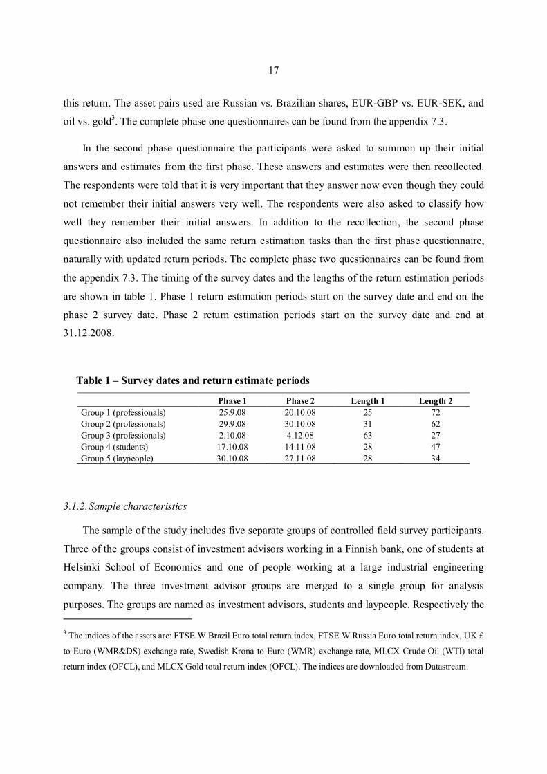
the appendix 7.3. The timing of the survey dates and the lengths of the return estimation periods
are shown in table 1. Phase 1 return estimation periods start on the survey date and end on the
phase 2 survey date. Phase 2 return estimation periods start on the survey date and end at
31.12.2008.
Table 1 – Survey dates and return estimate periods
Phase 1 Phase 2 Length 1 Length 2
Group 1 (professionals) 25.9.08 20.10.08 25 72
Group 2 (professionals) 29.9.08 30.10.08 31 62
Group 3 (professionals) 2.10.08 4.12.08 63 27
Group 4 (students) 17.10.08 14.11.08 28 47
Group 5 (laypeople) 30.10.08 27.11.08 28 34
3.1.2. Sample characteristics
The sample of the study includes five separate groups of controlled field survey participants.
Three of the groups consist of investment advisors working in a Finnish bank, one of students at
Helsinki School of Economics and one of people working at a large industrial engineering
company. The three investment advisor groups are merged to a single group for analysis
purposes. The groups are named as investment advisors, students and laypeople. Respectively the
3 The indices of the assets are: FTSE W Brazil Euro total return index, FTSE W Russia Euro total return index, UK £
to Euro (W MR&DS) exchange rate, Swedish Krona to Euro (W MR) exchange rate, MLCX Crude Oil (W TI) total
return index (OFCL), and MLCX Gold total return index (OFCL). The indices are downloaded from Datastream.
18
sizes of the groups are: 56 investment advisors, 89 students, and 55 laypeople. Thus the total
sample size is 200.
The overall sample includes 104 men, 95 women and 1 who did not want to reveal his/her
sex. The respective distributions within the groups are 20 + 35 (+1) investment advisers, 61 + 28
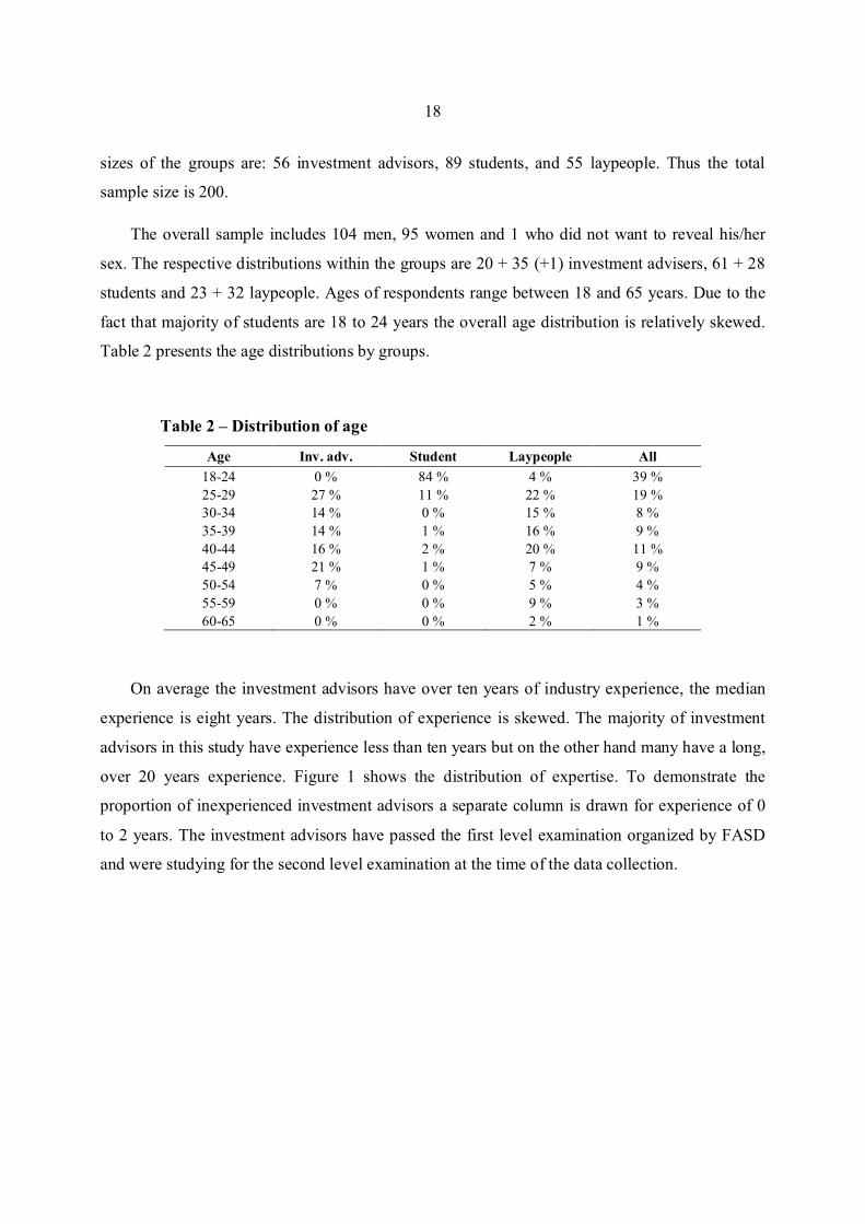
students and 23 + 32 laypeople. Ages of respondents range between 18 and 65 years. Due to the
fact that majority of students are 18 to 24 years the overall age distribution is relatively skewed.
Table 2 presents the age distributions by groups.
Table 2 – Distribution of age
Age Inv. adv. Student Laypeople All
18-24 0 % 84 % 4 % 39 %
25-29 27 % 11 % 22 % 19 %
30-34 14 % 0 % 15 % 8 %
35-39 14 % 1 % 16 % 9 %
40-44 16 % 2 % 20 % 11 %
45-49 21 % 1 % 7 % 9 %
50-54 7 % 0 % 5 % 4 %
55-59 0 % 0 % 9 % 3 %
60-65 0 % 0 % 2 % 1 %
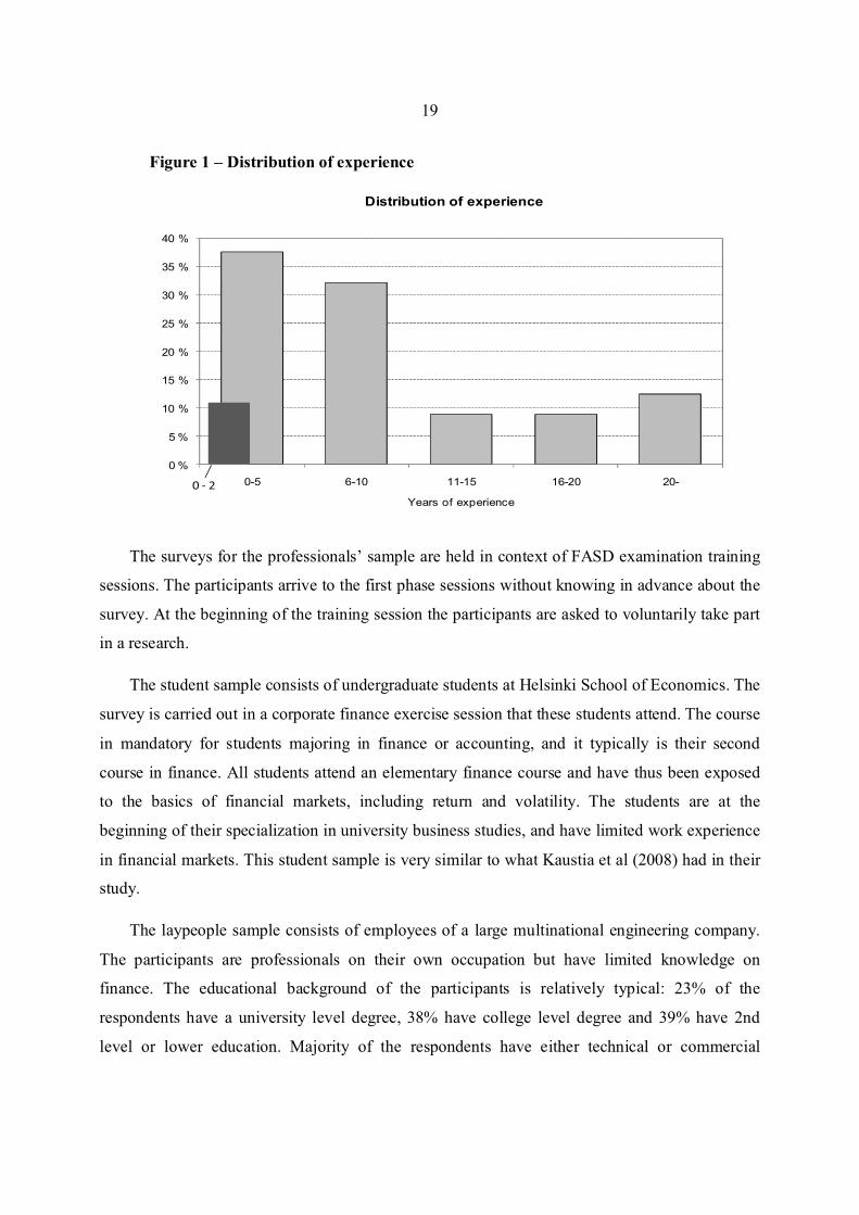
On average the investment advisors have over ten years of industry experience, the median
experience is eight years. The distribution of experience is skewed. The majority of investment
advisors in this study have experience less than ten years but on the other hand many have a long,
over 20 years experience. Figure 1 shows the distribution of expertise. To demonstrate the
proportion of inexperienced investment advisors a separate column is drawn for experience of 0
to 2 years. The investment advisors have passed the first level examination organized by FASD
and were studying for the second level examination at the time of the data collection.
19
Figure 1 – Distribution of experience
0 %
5 %
10 %
15 %
20 %
25 %
30 %
35 %
40 %
0-5 6-10 11-15 16-20 20-
Years of experience
Distribution of experience
0 -2
The surveys for the professionals’ sample are held in context of FASD examination training
sessions. The participants arrive to the first phase sessions without knowing in advance about the
survey. At the beginning of the training session the participants are asked to voluntarily take part
in a research.
The student sample consists of undergraduate students at Helsinki School of Economics. The
survey is carried out in a corporate finance exercise session that these students attend. The course
in mandatory for students majoring in finance or accounting, and it typically is their second
course in finance. All students attend an elementary finance course and have thus been exposed
to the basics of financial markets, including return and volatility. The students are at the
beginning of their specialization in university business studies, and have limited work experience
in financial markets. This student sample is very similar to what Kaustia et al (2008) had in their
study.
The laypeople sample consists of employees of a large multinational engineering company.
The participants are professionals on their own occupation but have limited knowledge on
finance. The educational background of the participants is relatively typical: 23% of the
respondents have a university level degree, 38% have college level degree and 39% have 2nd
level or lower education. Majority of the respondents have either technical or commercial

20
education: 39% have commercial education, 36% have technical and only 25% have some other
education. The sample includes participants from numerous organizational positions (e.g. senior
vice president, customer service employee and product responsible engineer).
The collection of the student and laypeople samples differ a little from the collection of
professional sample. Similarly to professional sample the participants arrive to the exercise
session / monthly briefing without prior information about the survey. For practical reasons the
questionnaires are dealt at the beginning of the session even though the actual time reserved for
the survey is at the end of the session. At the beginning the participants are briefly told the
purpose of the questionnaire and that there is time reserved for filling at the end of the session.
The survey is conducted after the normal agenda. The participants are instructed for the
questionnaire and told about the second phase. However the participants are not specifically
asked to remember their answers for the second phase. The participants are also told that all are
given a small reward for participating4. The setting for second phase is similar to the first phase,
with the exception that the participants know about the coming survey.
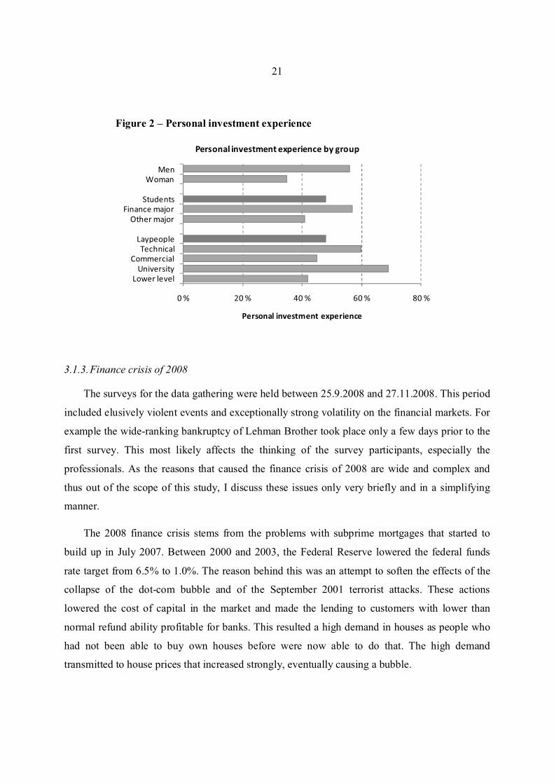
The students and laypeople were asked if they have made stock market transactions
themselves. In total 48% of non-professionals had made personal stock market transactions.
There is no difference between students and laypeople. However, men have more personal
experience in stock market investments; 56% of men have made transactions whereas only 35%
of women have. Also the major (students) and education (laypeople) affects; 57% of students
with finance major have personal experience but only 41% students with other major have.
W ithin the laypeople sample 60% of respondents with technical education has personal
investment experience. The respective proportion for respondents with commercial education is
45%. This rather surprising observation partly results from the fact that only 23% of commercial
employees have university degree whereas 35% of technical employees have university degree.
People with university degree generally are in higher positions in work organizations and thus
have more funds to invest. Accordingly, 69% of respondents with university degree have
personal investment experience. The respective proportion of people with lower level of
education is 42%. Figure 2 presents the results in graphical form.
4 All participants receive a stock market related card game at the second phase session.
21
Figure 2 – Personal investment experience
0 % 20 % 40 % 60 % 80 %
Low er level
University
Com m ercial
Technical
Laypeople
O ther m ajor
Finance m ajor
Students
W om an
M en
Personal investment experience
Personal investment experience by group
3.1.3. Finance crisis of 2008
The surveys for the data gathering were held between 25.9.2008 and 27.11.2008. This period
included elusively violent events and exceptionally strong volatility on the financial markets. For
example the wide-ranking bankruptcy of Lehman Brother took place only a few days prior to the
first survey. This most likely affects the thinking of the survey participants, especially the
professionals. As the reasons that caused the finance crisis of 2008 are wide and complex and
thus out of the scope of this study, I discuss these issues only very briefly and in a simplifying
manner.
The 2008 finance crisis stems from the problems with subprime mortgages that started to
build up in July 2007. Between 2000 and 2003, the Federal Reserve lowered the federal funds
rate target from 6.5% to 1.0%. The reason behind this was an attempt to soften the effects of the
collapse of the dot-com bubble and of the September 2001 terrorist attacks. These actions
lowered the cost of capital in the market and made the lending to customers with lower than
normal refund ability profitable for banks. This resulted a high demand in houses as people who
had not been able to buy own houses before were now able to do that. The high demand
transmitted to house prices that increased strongly, eventually causing a bubble.
22
The mortgages granted to subprime debtors were mainly securitized and diversified to a wide
range of financial market participants. These financial agreements known as mortgage-backed
securities (MBS), which derive their value from mortgage payments and housing prices, became
more and more common. The market for the MBS’s worked properly as long the housing prices
increased, however problems started to build up as prices started to decline and repayment
failures increased. The values of MBS’s started to deteriorate sharply and the holders had to
report losses. The fact that MBS’s are difficult to value and have low transparency caused a
situation where the holders of MBS’s were not able to explicitly report the value of their
holdings. This caused a market wide lack of thrust and froze the interbank debt market. This
resulted in a liquidity crisis.
Insufficient liquidity was the single most important reason behind the bankruptcies of e.g.
Bear Stearns (March 2008), Lehman Brothers and AIG (September 2008). Even though financial
institutions faced significant losses from subprime mortgages the lack of thrust and thus
negligible liquidity was the reason that made those to collapse. The market wide shortage of
liquidity increased the cost of capital dramatically and thus diminished the investments and
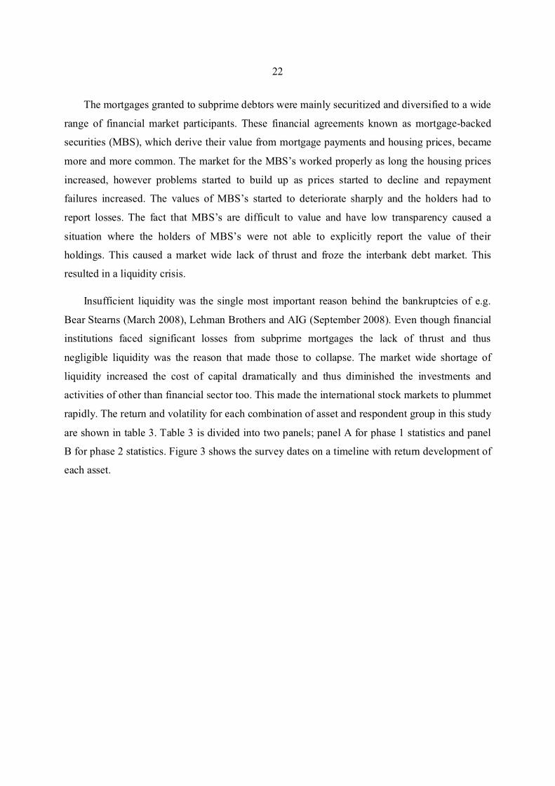
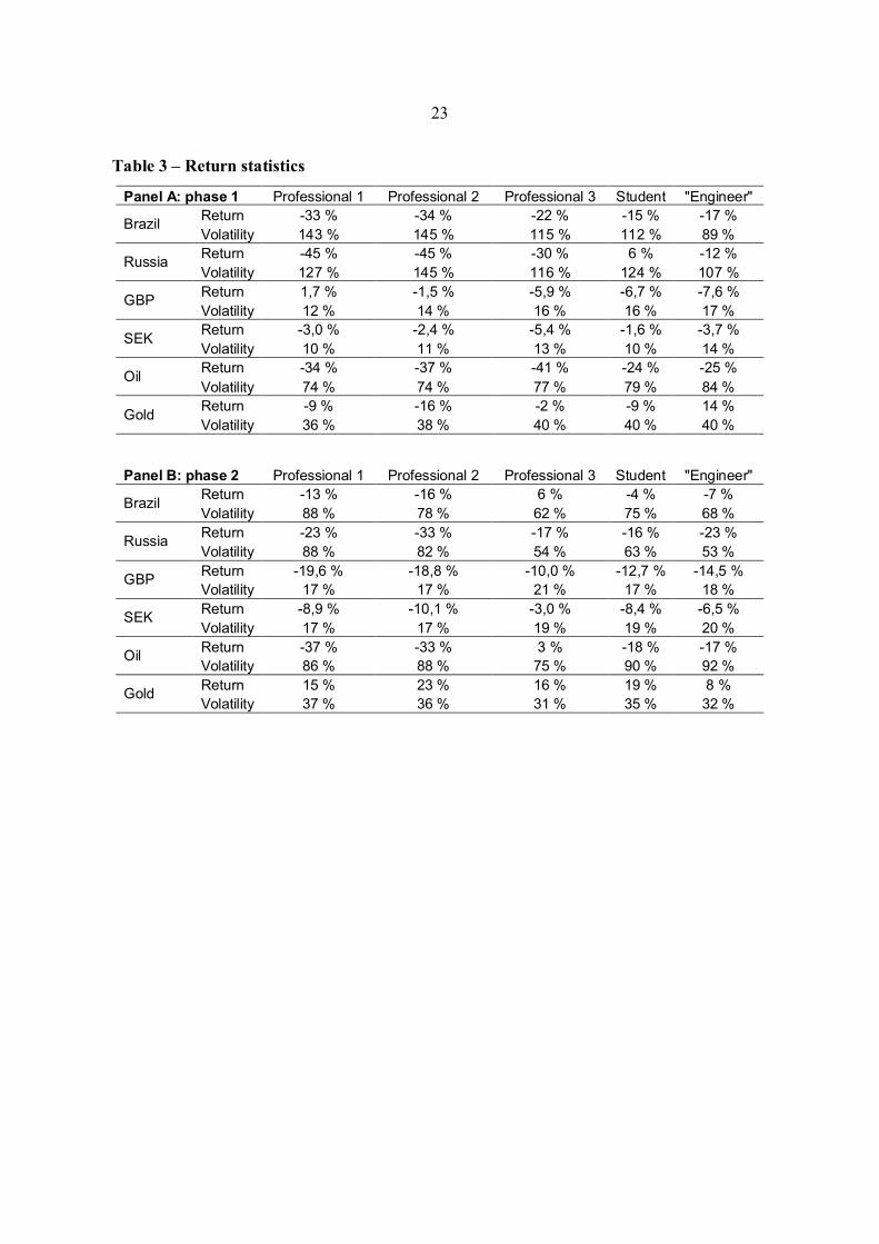
activities of other than financial sector too. This made the international stock markets to plummet
rapidly. The return and volatility for each combination of asset and respondent group in this study
are shown in table 3. Table 3 is divided into two panels; panel A for phase 1 statistics and panel
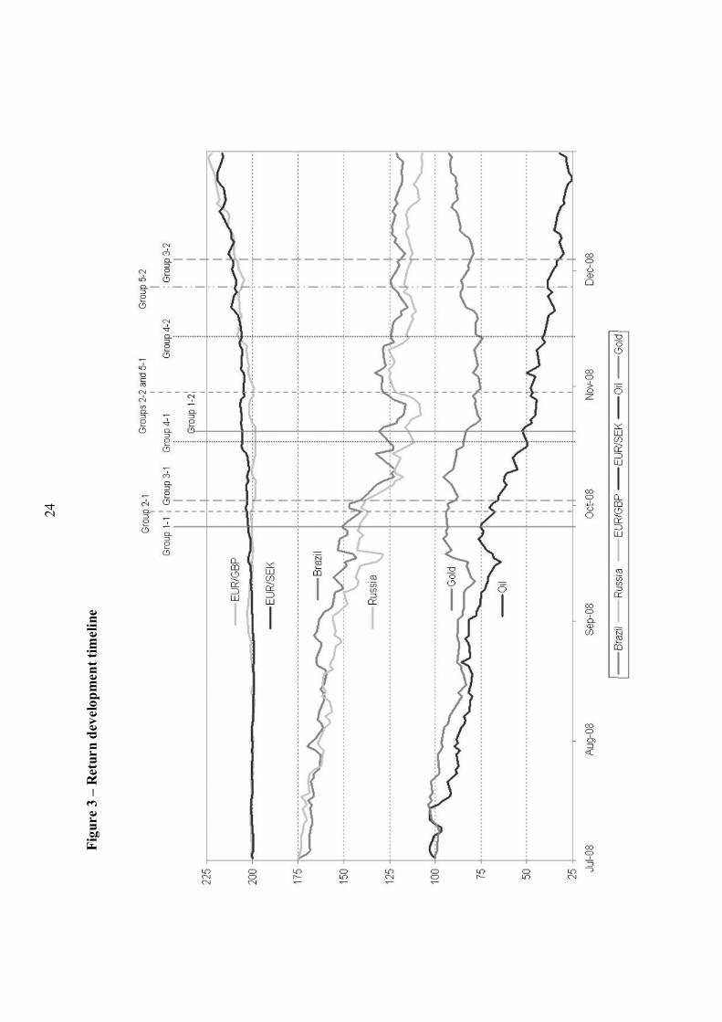
B for phase 2 statistics. Figure 3 shows the survey dates on a timeline with return development of
each asset.
23
Table 3 – Return statistics
Panel A: phase 1 Professional 1 Professional 2 Professional 3 Student "Engineer"
Brazil Return -33 % -34 % -22 % -15 % -17 %
Volatility 143 % 145 % 115 % 112 % 89 %
Russia Return -45 % -45 % -30 % 6 % -12 %
Volatility 127 % 145 % 116 % 124 % 107 %
GBP Return 1,7 % -1,5 % -5,9 % -6,7 % -7,6 %
Volatility 12 % 14 % 16 % 16 % 17 %
SEK Return -3,0 % -2,4 % -5,4 % -1,6 % -3,7 %
Volatility 10 % 11 % 13 % 10 % 14 %
Oil Return -34 % -37 % -41 % -24 % -25 %
Volatility 74 % 74 % 77 % 79 % 84 %
Gold Return -9 % -16 % -2 % -9 % 14 %
Volatility 36 % 38 % 40 % 40 % 40 %
Panel B: phase 2 Professional 1 Professional 2 Professional 3 Student "Engineer"
Brazil Return -13 % -16 % 6 % -4 % -7 %
Volatility 88 % 78 % 62 % 75 % 68 %
Russia Return -23 % -33 % -17 % -16 % -23 %
Volatility 88 % 82 % 54 % 63 % 53 %
GBP Return -19,6 % -18,8 % -10,0 % -12,7 % -14,5 %
Volatility 17 % 17 % 21 % 17 % 18 %
SEK Return -8,9 % -10,1 % -3,0 % -8,4 % -6,5 %
Volatility 17 % 17 % 19 % 19 % 20 %
Oil Return -37 % -33 % 3 % -18 % -17 %
Volatility 86 % 88 % 75 % 90 % 92 %
Gold Return 15 % 23 % 16 % 19 % 8 %
Volatility 37 % 36 % 31 % 35 % 32 %
24
Fig
ure 3
– R
etu
rn
dev
elo
pm
en
t ti
meli
ne

25
3.2. Methods
In this chapter I discuss the methods used in the empirical study. The data gathered in the
controlled field surveys enables a wide range of analyses to be carried out. The structure of the
survey makes it possible to study the three biases in question. The main insight in formulating the
tests described in this section is to compare the observations from different phases of the surveys
to each other. Hindsight bias is observed by differences between initial answers and the
recollections. Overconfidence is studied using initial answers and realized results. Analyses of
self-attribution bias use initial answers from first and second round.
3.2.1. Hindsight bias
In this study the effects of hindsight bias are examined in four aspects of behavior. The tests
are designed to versatilely utilize the data collected in the survey. The underlying logic for all of
the four tests is the main attribute of hindsight bias; people tend to percept their own initial
behavior as more optimal than it actually is after learning the future.
3.2.1.1. Asset selection effect
The first aspect is to study if remembering own selection in a winner selection task is
unbiased. This is called ‘asset selection effect’. Asset selection effect refers to an attribute of
hindsight bias where people tend to remember their initial selection incorrectly in a task where
they are asked to select a winner from two alternatives. After learning the outcome hindsight
biased agents remember that they chose the winning asset even though it may not be true.
The logic behind the asset selection test of this study is based to the effect where hindsight
biased agents fail to recognize a failure in a winner selection task, like the one in this study. The
tendency of overestimating own success is measured by comparing the actual proportion of
correct answers and the respective remembered proportion. Thus this analysis uses the initial
selections, the recollections of the initial selections and the realized results from the
questionnaire. Naturally some proportion of the recollections is incorrect simply because the
respondent has forgotten his/her initial selection. However, these falsely remembered answers
26
should distribute randomly and irrespective of the outcome and thus should not affect the results
related to hindsight bias.
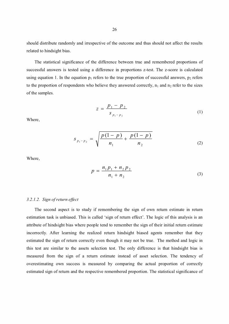
The statistical significance of the difference between true and remembered proportions of
successful answers is tested using a difference in proportions z-test. The z-score is calculated
using equation 1. In the equation p1 refers to the true proportion of successful answers, p2 refers
to the proportion of respondents who believe they answered correctly, n1 and n2 refer to the sizes
of the samples.
(1)
W here,
(2)
W here,
(3)
3.2.1.2. Sign of return effect
The second aspect is to study if remembering the sign of own return estimate in return
estimation task is unbiased. This is called ‘sign of return effect’. The logic of this analysis is an
attribute of hindsight bias where people tend to remember the sign of their initial return estimate
incorrectly. After learning the realized return hindsight biased agents remember that they
estimated the sign of return correctly even though it may not be true. The method and logic in
this test are similar to the assets selection test. The only difference is that hindsight bias is
measured from the sign of a return estimate instead of asset selection. The tendency of
overestimating own success is measured by comparing the actual proportion of correctly
estimated sign of return and the respective remembered proportion. The statistical significance of
21
21
pps
ppz
"
"#
21
)1()1(21 n
pp
n
pps pp
"$
"#"
21
2211
nn
pnpnp
$
$#
27
the difference between true and remembered proportions of correct sign of return is tested using
the exact same difference in proportions z-test as in asset selection test.
3.2.1.3. Drift of return effect
The third aspect is to study a tendency of remembering own initial estimates to be closer to
the realized figures than they actually are (i.e. moving closer to realized). This is done by
comparing the actual return estimates, the recollections of the actual estimates, and the realized
returns. In this design the subjects are first asked to report their ex-ante expectations at the first
phase of the survey. Then, they learn the realization of the return at the second phase. Finally
they are asked to report their ex-post recollection of their ex-ante expectations.
The difference between the initial return estimate and the recollection is calculated for each
respondent. To demonstrate hindsight bias the sample is divided into two groups based on the
initial answer – realization relationship. Such answers in which the initial estimate is higher than
the realized result form the first group. Answers in which the initial estimate is lower than the
realized result form the other group. The logic in this structure is to separate the answers based on
which direction the ‘drift’ is likely to affect.
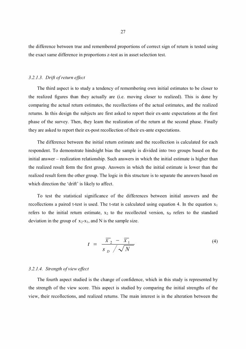
To test the statistical significance of the differences between initial answers and the
recollections a paired t-test is used. The t-stat is calculated using equation 4. In the equation x1
refers to the initial return estimate, x2 to the recollected version, sD refers to the standard
deviation in the group of x2-x1, and N is the sample size.
(4)
3.2.1.4. Strength of view effect
The fourth aspect studied is the change of confidence, which in this study is represented by
the strength of the view score. This aspect is studied by comparing the initial strengths of the
view, their recollections, and realized returns. The main interest is in the alteration between the
Ns
xxt
D
12 "#
28
initial strength of view and the recollection, not in the actual level of confidence. To demonstrate
hindsight bias the sample is divided into two groups based on success of the asset selection task.
The other group is the ones with believed correct answer and the other is the ones with believed
incorrect answer. The logic behind this is an attribute of hindsight bias according to which people
that believe they answered correctly may overestimate their initial certainty and people that
believe they answered incorrectly may underestimate it. The difference between the initial
strength of view and the recollection is tested and the statistical significance is determined using
the same paired t-test method as in drift of return test.
3.2.2. Overconfidence
Overconfidence is studied in two sets of tests. The first set of tests observes the ‘setting too
narrow limits’ –effect by examining how the respondents estimate volatility. The second set of
tests observes the relation between perceived confidence and actual ability to success in asset
selection task.
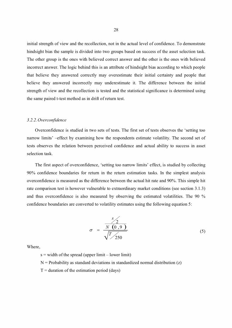
The first aspect of overconfidence, ‘setting too narrow limits’ effect, is studied by collecting
90% confidence boundaries for return in the return estimation tasks. In the simplest analysis
overconfidence is measured as the difference between the actual hit rate and 90%. This simple hit
rate comparison test is however vulnerable to extraordinary market conditions (see section 3.1.3)
and thus overconfidence is also measured by observing the estimated volatilities. The 90 %
confidence boundaries are converted to volatility estimates using the following equation 5:
(5)
W here,
s = width of the spread (upper limit – lower limit)
N = Probability as standard deviations in standardized normal distribution (z)
T = duration of the estimation period (days)
% &
250
9,02
T
N
s
#'

29
The fact that the surveys were held on different dates and the estimation periods were
unequally lengthy makes accurate volatilities difficult to calculate. Also the sample sizes for
separate asset – return period combinations would be very small. For these reasons a simplified
analysis is carried out. In this analysis the three investment advisor groups are pooled together
and the volatilities for each asset class are calculated by averaging the individual volatilities of an
asset-time combination. Student and laypeople samples are issued separately but the volatilities
for each asset class are also calculated with the same method. These converted and averaged
volatility estimates are compared to realized and previous volatilities.
The second set of overconfidence analyses uses a logit-regression to forecast success in
picking the better performing asset. Logit-regression is a convenient way to demonstrate the
effects of certain variables on a probability to succeed in a binary task. For the purpose of this
study logit-regression is appropriate method to study which factors contribute to the probability
that a respondent chooses the better performing asset from the two alternatives. The regression
uses the binary variable of success as the response (dependent) variable. The used explanatory
(independent) variables for the regression are determined based on the collected background
information. In addition to background information the strength of view score is used in the
regression. The main interest in the regression analysis is to study the effect of confidence
(strength of view score) on performance. A negative impact on the probability to succeed would
be a strong sign of overconfidence. Also the independency of success from strength of view is
interpreted as overconfidence.
The statistical significance of the regression coefficients is tested using a W ald test. The
W ald score is calculated using equation 6. The score is compared against a chi-square
distribution.
(6)
W here,
^� = the maximum likelihood estimate of an variable
�0 = Proposed value of the variable ( 0 )
)ˆ(
)ˆ( 2
0
(
((
Varw
"#
30
As the relation of confidence and success is studied and existence of overconfidence is
determined based on this relation, it is important to study factors affecting confidence. For this
reason an ordinary least square regression is carried. The purpose of this regression is to discover
factors affecting confidence. An increase in confidence for some variable while the same variable
lowers performance, indicate overconfidence. Thus the results of this OLS-regression are
compared to results of the logit-regression. The regression uses the strength of view score as the
response (dependent) variable for confidence. The used explanatory (independent) variables are
gender, profession and the thinking style scores NFC and FI. The significance of the results is
demonstrated using standard t-test.
3.2.3. Self-attribution bias
The effects self-attribution bias of are studied in two tests. Both tests measure self-attribution
bias by the change in perceived certainty of success between first and second rounds. The
difference is in the determination of success. First test uses individual answers whereas second
test uses pooled answers for a single person.
In the first test a respondent’s recollected certainty (strength of view score) of an individual
task at phase 1 is compared to the given certainty to the repetition of the same task. Self-
attribution bias is determined by the difference between these scores. The analysis uses
recollection instead of initial strength of view score to eliminate effects of hindsight bias to this
analysis. To demonstrate self-attribution bias the sample is divided into two, based on the
perceived correctness of the initial answer. The logic in this is an attribute of self-attribution bias
according to which people that believe to be successful attribute themselves on the success and
thus increase their confidence on a repetition of the task. On the contrary people who believe to
be unsuccessful may decrease their confidence on a repetition of the task. The statistical
significance of these differences is calculated using a similar paired t-test as with hindsight bias
analyses.
The second test is similar to the first test with exception that the respondents are categorized
into four groups based on how many correct answers they believe they had on the first round. The
change of confidence in each group is observed using the same method of calculating the
31
difference in the strength of view score between phase 1 (recollection) and phase 2. Also
similarly to other tests in this study, the significance of the differences is calculated using a paired
t-test.
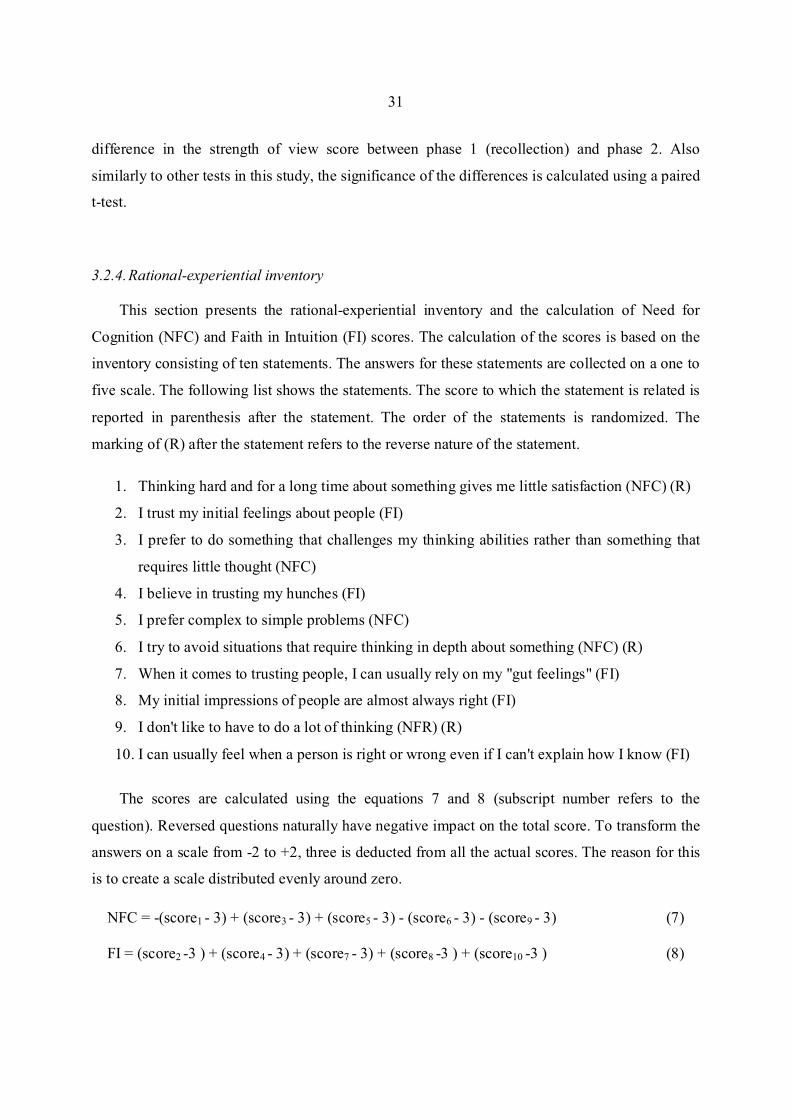
3.2.4. Rational-experiential inventory
This section presents the rational-experiential inventory and the calculation of Need for
Cognition (NFC) and Faith in Intuition (FI) scores. The calculation of the scores is based on the
inventory consisting of ten statements. The answers for these statements are collected on a one to
five scale. The following list shows the statements. The score to which the statement is related is
reported in parenthesis after the statement. The order of the statements is randomized. The
marking of (R) after the statement refers to the reverse nature of the statement.
1. Thinking hard and for a long time about something gives me little satisfaction (NFC) (R)
2. I trust my initial feelings about people (FI)
3. I prefer to do something that challenges my thinking abilities rather than something that
requires little thought (NFC)
4. I believe in trusting my hunches (FI)
5. I prefer complex to simple problems (NFC)
6. I try to avoid situations that require thinking in depth about something (NFC) (R)
7. W hen it comes to trusting people, I can usually rely on my "gut feelings" (FI)
8. My initial impressions of people are almost always right (FI)
9. I don't like to have to do a lot of thinking (NFR) (R)
10. I can usually feel when a person is right or wrong even if I can't explain how I know (FI)
The scores are calculated using the equations 7 and 8 (subscript number refers to the
question). Reversed questions naturally have negative impact on the total score. To transform the
answers on a scale from -2 to +2, three is deducted from all the actual scores. The reason for this
is to create a scale distributed evenly around zero.
NFC = -(score1 - 3) + (score3 - 3) + (score5 - 3) - (score6 - 3) - (score9 - 3) (7)
FI = (score2 -3 ) + (score4 - 3) + (score7 - 3) + (score8 -3 ) + (score10 -3 ) (8)

32
4. Results
The results section presents the results from the tests described in section 3.2. In addition to
the plain presentation of the result I discuss the possible reasons behind the results and the
consequences. The interconnection between the biases and possibly explanatory characteristics is
also discussed. The first three subsections discuss the actual behavioral biases observed in this
study. These sections are considered as the main contribution of this study. In addition the results
from the psychological test are presented in the last subsection.
As investment advisors are the most important sample of this study and stock market
estimates are most usual for investment advisors, separate analyses on investment advisors’ stock
market estimates are carried. For several of the tests, there are such extra analyses after the actual
results discussion. These analyses use the same methods as the actual tests but focus on the
impacts of professionals’ biases on their occupation.
4.1. Hindsight bias
The effects of hindsight bias are studied in four different tests. The results of the first two
tests, ‘asset selection’ and ‘sign of return’, are considered as main contribution of the hindsight
bias section of this study. However results from the latter two tests, drift of return and strength of
view also support the analysis of hindsight bias. The techniques used are discussed in more detail
in section 3.2.1.
4.1.1. Asset selection effect
Asset selection effect refers to an attribute of hindsight bias where people remember their
initial selection incorrectly in a task where they are asked to select a winner from two
alternatives. Hindsight biased agents remember that they chose the winning asset even though it
may not be true. In this study asset selection effect is tested by comparing the true and
remembered proportions of correct answers in the asset selection tasks. Table 4 shows the results
from the test. The purpose of table 4 is to show the initial selections in relation to recollected
versions of the selections. Thus both true and remembered proportions of successful answers in

33
the asset selection tasks are shown, as well as the difference. To discover the statistical
significance of the results a difference on proportions z-test is carried out. ‘True’ sample consists
of all answers that included the selection of asset and the ‘remembered’ sample consists of all
answers that included the selection of asset and the recollection. Thus the total sample sizes are
588 and 367. The sizes of the subsamples may vary depending on the number of rejected answers
sheets.
34
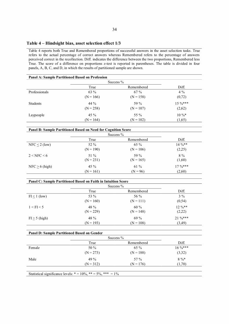
Table 4 – Hindsight bias, asset selection effect 1/3
Table 4 reports both True and Remembered proportions of successful answers in the asset selection tasks. True refers to the actual percentage of correct answers whereas Remembered refers to the percentage of answers perceived correct in the recollection. Diff. indicates the difference between the two proportions, Remembered less True. The score of a difference on proportions z-test is reported in parentheses. The table is divided in four panels, A, B, C, and D, in which the results of partitioned sample are shown.
Panel A: Sample Partitioned Based on Profession
Success %
True Remembered Diff.
Professionals 63 % 67 % 4 %
(N = 166) (N = 158) (0,72) Students 44 % 59 % 15 %***
(N = 258) (N = 107) (2,62) Laypeople 45 % 55 % 10 %*
(N = 164) (N = 102) (1,65)
Panel B: Sample Partitioned Based on Need for Cognition Score
Success %
True Remembered Diff.
NFC < 2 (low) 52 % 65 % 14 %**
(N = 190) (N = 106) (2,25)
2 < NFC < 6 51 % 59 % 8 % (N = 231) (N = 165) (1,60)
NFC > 6 (high) 45 % 61 % 17 %***
(N = 161) (N = 96) (2,60)
Panel C: Sample Partitioned Based on Faith in Intuition Score
Success %
True Remembered Diff.
FI < 1 (low) 53 % 56 % 3 %
(N = 160) (N = 111) (0,54)
1 < FI < 5 48 % 60 % 12 %**
(N = 229) (N = 148) (2,22)
FI > 5 (high) 48 % 69 % 21 %***
(N = 193) (N = 108) (3,49)
Panel D: Sample Partitioned Based on Gender
Success %
True Remembered Diff.
Female 50 % 65 % 16 %***
(N = 273) (N = 188) (3,32) Male 49 % 57 % 8 %*
(N = 312) (N = 176) (1,70)
Statistical significance levels: * = 10%, ** = 5%, *** = 1%
35
All partitions of the sample show a positive effect in change between remembered and true
rate of success. However, for some partitions the difference is not statistically significant. Panel
A shows the results for each respondent group. The professionals sample shows only a 4 %
difference which is not statistically significant even at 10 percent significance level (z = 0.72).
Students sample shows a 15 percent difference that is highly significant (z = 2.62, p < 0.01).
Laypeople sample shows a 10 percent difference that is significant at 10 percent significance
level (z = 1.65). Based on these results professionals seem to be the least exposed and student the
most exposed group, laypeople lay in between. The fact that professionals are least exposed to
asset selection effect supports the hypothesis that expertise reduces behavioral biases. However,
the support is only weak as students show stronger exposure than laypeople, although the
hypothesis that students possess more expertise than so called laypeople is not a strong one.
The effect of individual thinking style on asset selection effect is not unambiguous. The
Need for Cognition (NFC) score, that represents analytical thinking, does not explain asset
selection effect linearly. Panel B presents that both high and low NFC-score partitions show
statistically significant difference between true and remembered success rates but not for the
middle partition. The low 30 percent NFC sample shows a 14 percent difference that is
significant at 5 percent significance level (z = 2.25). The middle 40 percent sample shows an 8
percent difference (z = 1.60). The high 30 percent sample shows a 17 percent difference that is
highly significance (z = 2.60, p < 0.01). These results do not support the hypothesis that
analytical thinking reduces behavioral biases.
Unlike analytical thinking, faith in intuition shows a straightforward relationship between
asset selection effect and individual thinking style. Faith in Intuition (FI) score seems to explain
asset selection effect linearly. Panel C shows the results from tests on sample partitioned based
on FI-score. The low 30 percent FI sample shows only a 3 percent difference between true and
remembered success rates. The difference is not significant even at 10 percent significance level
(z = 0.54). The middle 40 percent sample shows a 12 percent difference that is significant at 5
percent level (z = 2.22). Finally the high 30 percent sample shows up to 21 percent difference
that is highly significant (z = 3.49, p < 0.01). The results in panel C imply that there is a strong
relationship between faith in intuition and behavioral biases.
36
Also a gender-effect seems to exist. Panel D shows the results partitioned by gender. The
female sample shows a 16 percent difference between true and remembered success rates. The
difference is highly significant (z = 3.32, p < 0.01). The respective difference for men is 8 percent
which is significant at 10 percent significance level (z = 1.70).
Overall the results in table 4 indicate that people find themselves succeeding more often they
actually do. This supports the evidence that people suffer from hindsight bias. I find that this
effect represents a strong form of hindsight bias. It requires more ‘I knew it all along’ kind of
thinking to alter one’s binary choice of selection than simply adjust a linear estimate to meet the
realization. The chosen asset is also more concrete and thus easier to remember than a return
estimate in a number format. In a binary selection task the subject can only make a right or wrong
choice.
Another issue that can be seen from table 4 is the performance of each group. The
performance is measured as the percentage of total correct answers not depending whether it is
correctly remembered. The professionals are correct in 63 % of tasks, students 44 % and
laypeople 45 %. As simple coin toss is correct 50% of times, the only group outperforming pure
randomness is the professionals group.
The results in panel A of table 4 support the hypothesis that expertise reduces behavioral
biases. However the fact that students, that are hypothesized to posses more expertise than
laypeople, seem to be the most exposed group raises a question on the sub-profession differences
on expertise. To answer this question a further analysis on experience is also carried out. Table 5
reports the same difference between true and remembered success rates as table 4, with the
exception that each of the profession samples are further partitioned based on expertise related
variables.
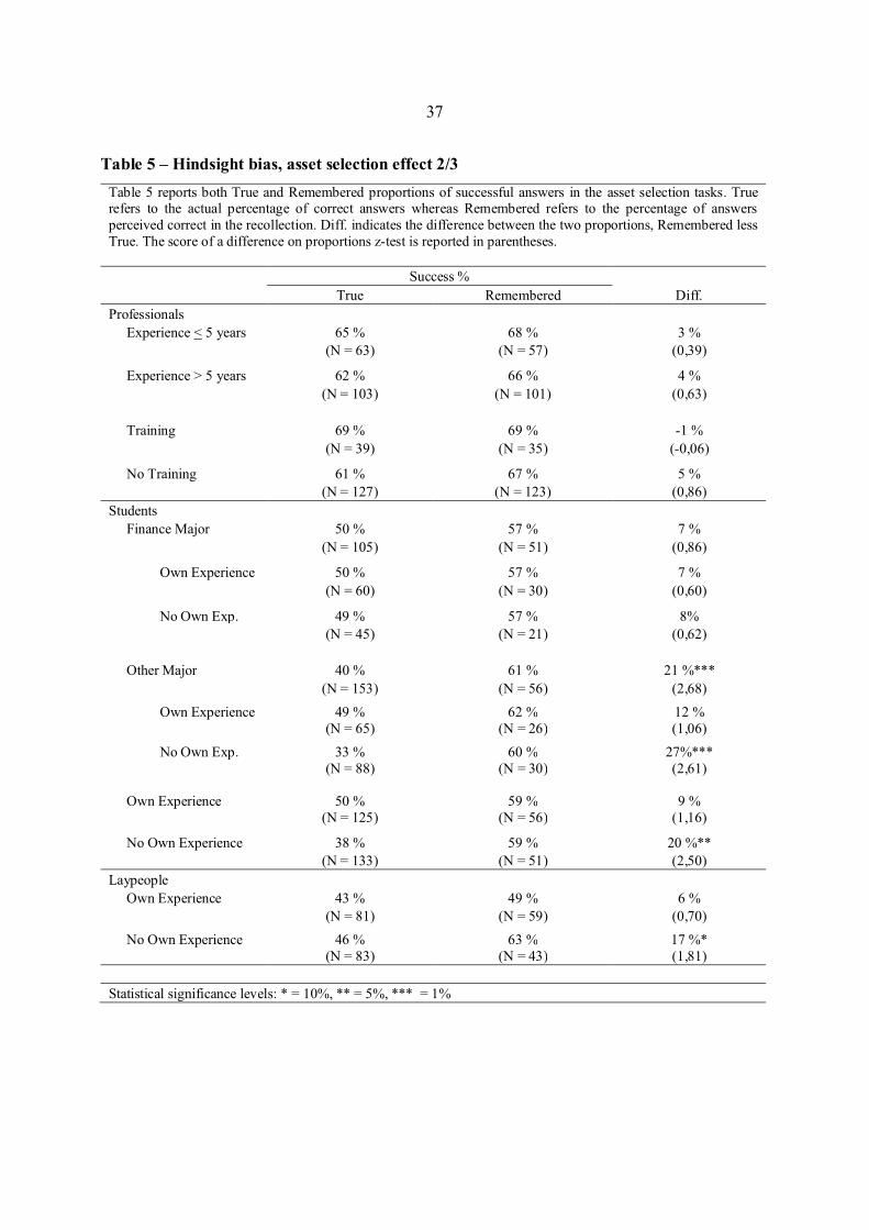
37
Table 5 – Hindsight bias, asset selection effect 2/3
Table 5 reports both True and Remembered proportions of successful answers in the asset selection tasks. True refers to the actual percentage of correct answers whereas Remembered refers to the percentage of answers
perceived correct in the recollection. Diff. indicates the difference between the two proportions, Remembered less
True. The score of a difference on proportions z-test is reported in parentheses.
Success %
True Remembered Diff.
Professionals
Experience < 5 years 65 % 68 % 3 %
(N = 63) (N = 57) (0,39)
Experience > 5 years 62 % 66 % 4 %
(N = 103) (N = 101) (0,63)
Training 69 % 69 % -1 %
(N = 39) (N = 35) (-0,06)
No Training 61 % 67 % 5 %
(N = 127) (N = 123) (0,86)
Students
Finance Major 50 % 57 % 7 %
(N = 105) (N = 51) (0,86)
Own Experience 50 % 57 % 7 %
(N = 60) (N = 30) (0,60)
No Own Exp. 49 % 57 % 8%
(N = 45) (N = 21) (0,62)
Other Major 40 % 61 % 21 %***
(N = 153) (N = 56) (2,68)
Own Experience 49 % 62 % 12 %
(N = 65) (N = 26) (1,06)
No Own Exp. 33 % 60 % 27%***
(N = 88) (N = 30) (2,61)
Own Experience 50 % 59 % 9 %
(N = 125) (N = 56) (1,16)
No Own Experience 38 % 59 % 20 %**
(N = 133) (N = 51) (2,50)
Laypeople
Own Experience 43 % 49 % 6 %
(N = 81) (N = 59) (0,70)
No Own Experience 46 % 63 % 17 %*
(N = 83) (N = 43) (1,81)
Statistical significance levels: * = 10%, ** = 5%, *** = 1%
38
The sub-profession results of the professional sample are somewhat equal with each other
and in line with the total professional sample results. The difference between true and
remembered success rates for any of the four sub-groups is not statistically significant even at 10
percent significance level. A minor difference is in training variable. Those professionals who
have participated in a behavioral finance seminar (prior to the survey session), show a practically
0 percent difference between true and remembered success rates (z = -0.06). However, the
respective difference for professionals who have not participated in such seminar is 5 percent
which is not significant (z = 0.86). Even though the observation is weak, it supports the
hypothesis that expertise reduces behavioral biases.
The sub-profession results of the student and laypeople samples seem to be rather volatile for
segregation based on expertise. In the student sample major of the respondent and personal
investment experience seem to explain the exposure to asset selection effect well. Students
studying finance as their major have a 7 percent difference between true and remembered success
rates, which is not significant (z = 0.86). On the contrary students with other than finance major
show a 21 percent difference, which is highly significant (z = 2.68, p < 0.01). In a similar vein
students that have personal investment experience show a 9 percent difference, which is not
significant (z = 1.16). Students who do not have personal investment experience show a 20
percent difference, which is significant at 5 percent significance level (z = 2.50). These results
support the hypothesis that expertise and experience reduce behavioral biases.
Similarly to the student sample, the sub-profession results of the laypeople sample are
affected by personal investment experience. Respondents that have personal investment
experience show only a 6 percent difference between true and remembered success rates. This
difference is not significant even at ten percent significance level (z = 0.70). On the contrary
respondents that do not have personal investment experience show a 17 percent difference, which
is significant at 10 percent significance level (z= 1.81). Also these results support the hypothesis
that experience reduces behavioral biases.
Overall the results in table 5 support the hypothesis that expertise reduces behavioral biases.
However, if expertise truly reduces behavioral biases, the hypothesis that students posses more
expertise that so called laypeople cannot be accepted per se. The results in table 5 show that there
are significant differences inside student and laypeople samples. This suggests that considering
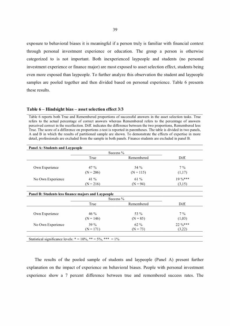
39
exposure to behavioral biases it is meaningful if a person truly is familiar with financial context
through personal investment experience or education. The group a person is otherwise
categorized to is not important. Both inexperienced laypeople and students (no personal
investment experience or finance major) are most exposed to asset selection effect, students being
even more exposed than laypeople. To further analyze this observation the student and laypeople
samples are pooled together and then divided based on personal experience. Table 6 presents
these results.
Table 6 – Hindsight bias – asset selection effect 3/3
Table 6 reports both True and Remembered proportions of successful answers in the asset selection tasks. True
refers to the actual percentage of correct answers whereas Remembered refers to the percentage of answers
perceived correct in the recollection. Diff. indicates the difference between the two proportions, Remembered less True. The score of a difference on proportions z-test is reported in parentheses. The table is divided in two panels, A and B in which the results of partitioned sample are shown. To demonstrate the effects of expertise in more
detail, professionals are excluded from the sample in both panels. Finance students are excluded in panel B.
Panel A: Students and Laypeople
Success %
True Remembered Diff.
Own Experience 47 % 54 % 7 %
(N = 206) (N = 115) (1,17)
No Own Experience 41 % 61 % 19 %***
(N = 216) (N = 94) (3,15)
Panel B: Students less finance majors and Laypeople
Success %
True Remembered Diff.
Own Experience 46 % 53 % 7 %
(N = 146) (N = 85) (1,03)
No Own Experience 39 % 62 % 22 %***
(N = 171) (N = 73) (3,22)
Statistical significance levels: * = 10%, ** = 5%, *** = 1%
The results of the pooled sample of students and laypeople (Panel A) present further
explanation on the impact of experience on behavioral biases. People with personal investment
experience show a 7 percent difference between true and remembered success rates. The
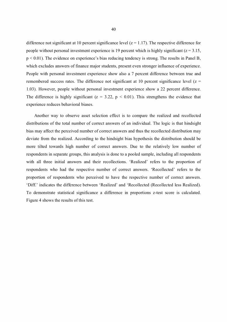
40
difference not significant at 10 percent significance level (z = 1.17). The respective difference for
people without personal investment experience is 19 percent which is highly significant (z = 3.15,
p < 0.01). The evidence on experience’s bias reducing tendency is strong. The results in Panel B,
which excludes answers of finance major students, present even stronger influence of experience.
People with personal investment experience show also a 7 percent difference between true and
remembered success rates. The difference not significant at 10 percent significance level (z =
1.03). However, people without personal investment experience show a 22 percent difference.
The difference is highly significant (z = 3.22, p < 0.01). This strengthens the evidence that
experience reduces behavioral biases.
Another way to observe asset selection effect is to compare the realized and recollected
distributions of the total number of correct answers of an individual. The logic is that hindsight
bias may affect the perceived number of correct answers and thus the recollected distribution may
deviate from the realized. According to the hindsight bias hypothesis the distribution should be
more tilted towards high number of correct answers. Due to the relatively low number of
respondents in separate groups, this analysis is done to a pooled sample, including all respondents
with all three initial answers and their recollections. ‘Realized’ refers to the proportion of
respondents who had the respective number of correct answers. ‘Recollected’ refers to the
proportion of respondents who perceived to have the respective number of correct answers.
‘Diff.’ indicates the difference between ‘Realized’ and ‘Recollected (Recollected less Realized).
To demonstrate statistical significance a difference in proportions z-test score is calculated.
Figure 4 shows the results of this test.
41
Figure 4 – Hindsight bias, asset selection effect
0 correct 1 correct 2 correct 3 correct
Realized 8,6 % 42,2 % 35,3 % 13,8 %
Recollected 3,4 % 31,0 % 47,4 % 18,1 %
Diff. -5,2 % -11,2 % 12,1 % 4,3 %
z-stat -1,65 -1,77 1,87 0,90
0 %
5 %
10 %
15 %
20 %
25 %
30 %
35 %
40 %
45 %
50 %Distribution of correct answers
As can be seen from figure 4 people tend to report a higher number of correct answers in the
recollection than they actually got right. This is in line with the hypothesis and also with the
results discussed above. There seems to be a verge of good and bad result between one and two
correct answers. People are reluctant to recognize the fact that they have only zero or one correct
answer and rather believe that they have two or three correct answers. Difference between true
and believed proportions for zero correct answers is -5.2%, which is significant at ten percent
significance level (z = -1.65). The respective difference for one correct answer is -11.2%, which
is also significant at ten percent significance level (z = -1.77). For two correct answers the
difference is positive, 12.1%. The difference is significant at ten percent level (z = 1.87). For
three correct answers the difference is 4.3%, which however is not significant (z = 0.90).
* * *
42
4.1.2. Sign of return effect
Sign of return effect refers to an attribute of hindsight bias where people remember the sign
of their initial return estimate incorrectly in a task where they are asked to predict the return of an
asset. Hindsight biased agents remember that they were able to predict the sign of the return
correctly even though it may not be true. Sign of return effect is tested by comparing the true
proportion of correctly estimated signs of return (‘True’) and remembered proportion of correct
sign of return (‘Remembered’) in return estimation task. Table 7 shows the results from the test.
The purpose of table 7 is to demonstrate the difference between ‘True’ and ‘Remembered’
proportions of correctly estimated signs of return. To discover the statistical significance of the
differences a difference on proportions z-test is carried out. The approach to this analysis is
similar to the asset selection analysis in section 4.1.1.
The conditions for answers to be included in sign of return sample are: firstly it contains the
selection of asset and the recollection; secondly it contains the return estimate and recollection in
correct format; and thirdly the recollection of asset selection is equal to the initial selection. The
reasons for first and second conditions are obvious, the reason for the third condition is in
eliminating the asset selection effect. Thus the sample size in the first phase is 428 and 264 in the
second phase. The sample consists of answers by 145 respondents.
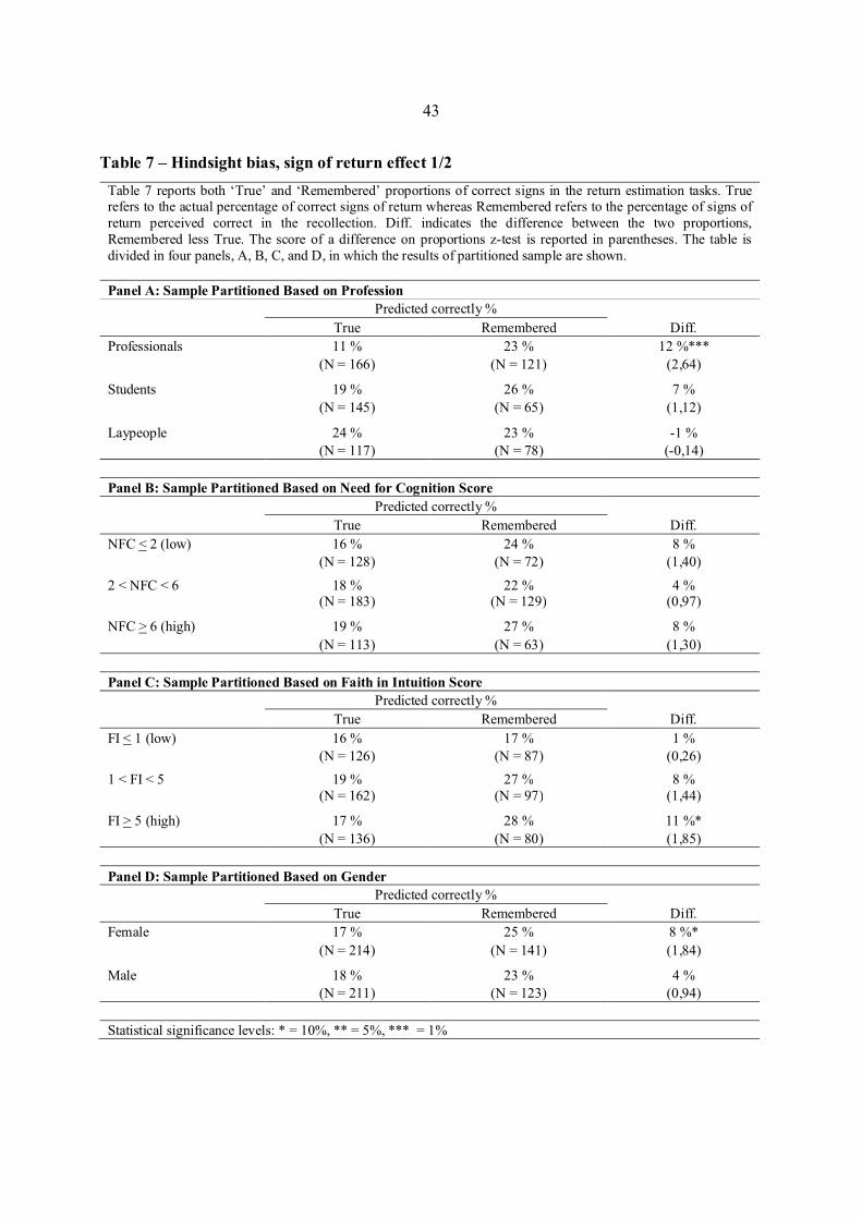
43
Table 7 – Hindsight bias, sign of return effect 1/2
Table 7 reports both ‘True’ and ‘Remembered’ proportions of correct signs in the return estimation tasks. True refers to the actual percentage of correct signs of return whereas Remembered refers to the percentage of signs of
return perceived correct in the recollection. Diff. indicates the difference between the two proportions,
Remembered less True. The score of a difference on proportions z-test is reported in parentheses. The table is
divided in four panels, A, B, C, and D, in which the results of partitioned sample are shown.
Panel A: Sample Partitioned Based on Profession
Predicted correctly %
True Remembered Diff.
Professionals 11 % 23 % 12 %***
(N = 166) (N = 121) (2,64)
Students 19 % 26 % 7 %
(N = 145) (N = 65) (1,12) Laypeople 24 % 23 % -1 %
(N = 117) (N = 78) (-0,14)
Panel B: Sample Partitioned Based on Need for Cognition Score
Predicted correctly %
True Remembered Diff.
NFC < 2 (low) 16 % 24 % 8 %
(N = 128) (N = 72) (1,40)
2 < NFC < 6 18 % 22 % 4 % (N = 183) (N = 129) (0,97)
NFC > 6 (high) 19 % 27 % 8 %
(N = 113) (N = 63) (1,30)
Panel C: Sample Partitioned Based on Faith in Intuition Score
Predicted correctly %
True Remembered Diff.
FI < 1 (low) 16 % 17 % 1 %
(N = 126) (N = 87) (0,26)
1 < FI < 5 19 % 27 % 8 %
(N = 162) (N = 97) (1,44)
FI > 5 (high) 17 % 28 % 11 %*
(N = 136) (N = 80) (1,85)
Panel D: Sample Partitioned Based on Gender
Predicted correctly %
True Remembered Diff.
Female 17 % 25 % 8 %*
(N = 214) (N = 141) (1,84) Male 18 % 23 % 4 %
(N = 211) (N = 123) (0,94)
Statistical significance levels: * = 10%, ** = 5%, *** = 1%

44
All partitions of the sample, excluding laypeople, show a positive effect in change between
remembered and true rate of success in estimating the sign of return. However, the differences are
statistically significant only for three subsamples. Panel A shows the results for each respondent
group. Interestingly professionals show the greatest difference between true and remembered
success rates. The professionals sample shows a 12 % difference which is statistically highly
significant (z = 2.64, p < 0.01). Students sample shows a 7 percent difference that is not
significant at 10 percent significance level (z = 1.12). Laypeople sample shows a -1 percent
difference that is not significant at 10 percent significance level (z = -0.14). The slightly negative
difference on laypeople can be interpreted as zero. The fact that professionals seem to be the most
exposed group can be partly explained by the timing of the surveys. As described in section 3.1
the market conditions were somewhat abnormal during the surveys, especially during the
professionals’ surveys. The realized returns of the assets in the professionals’ surveys were
negative in 17 out of 18 cases. The respective proportion for both students and laypeople is 1/6.
This combined to the fact that most of the estimates had a positive sign (92% of professionals,
80% of students, and 91% of laypeople) makes the comparison between respondent groups
difficult. The large proportion of positive signs under the prevailed market conditions is
interesting itself. It most likely results from optimism bias which however is not discussed here.
The incomparability of the groups does not however reduce the reliability of the finding that
investment advisors seem to have a tendency to perceive themselves being able to predict signs of
asset returns even though it might not be realistic.
The level of analytical thinking, measured by the Need for Cognition (NFC) score, does not
explain sign of return effect linearly. Panel B shows that both high and low NFC-score partitions
show higher difference between true and remembered success rates than the middle partition.
However, the difference is not significant for any of the groups. The low 30 percent NFC sample
shows an 8 percent difference (z = 1.40). The middle 40 percent sample shows a 4 percent
difference (z = 0.97). The high 30 percent sample shows an 8 percent difference (z = 1.30). These
results are in line with the results from the asset selection test and thus do not support the
hypothesis that analytical thinking reduces behavioral biases.
In contrast to analytical thinking, faith in intuition (FI) score seems to explain sign of return
effect linearly. Panel C shows the results from tests on sample partitioned based on FI-score. The
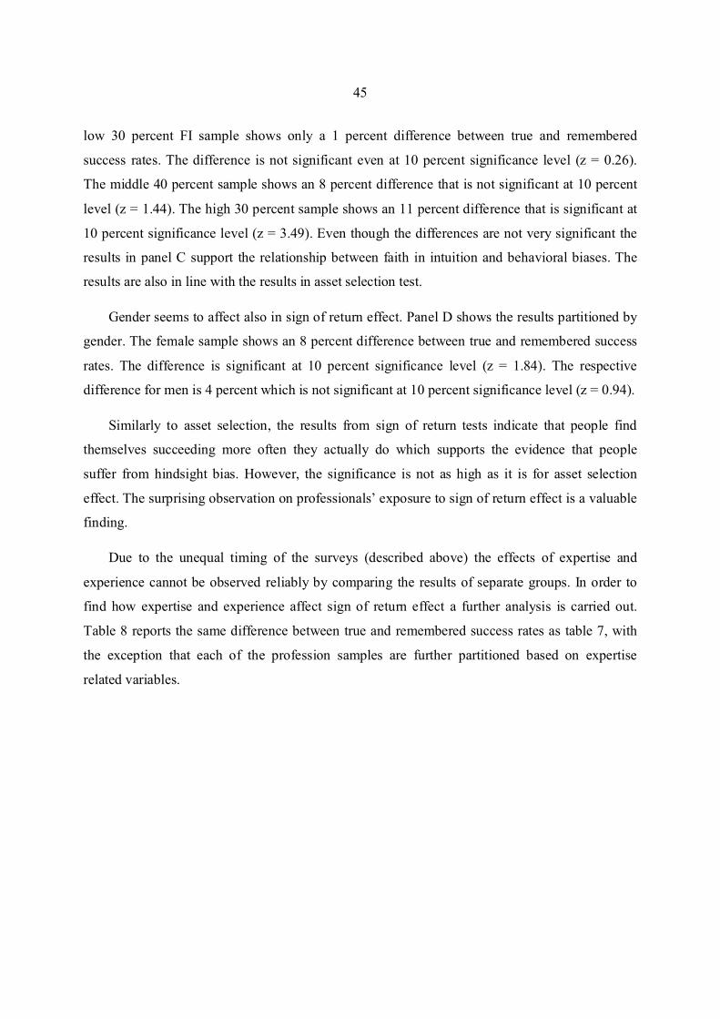
45
low 30 percent FI sample shows only a 1 percent difference between true and remembered
success rates. The difference is not significant even at 10 percent significance level (z = 0.26).
The middle 40 percent sample shows an 8 percent difference that is not significant at 10 percent
level (z = 1.44). The high 30 percent sample shows an 11 percent difference that is significant at
10 percent significance level (z = 3.49). Even though the differences are not very significant the
results in panel C support the relationship between faith in intuition and behavioral biases. The
results are also in line with the results in asset selection test.
Gender seems to affect also in sign of return effect. Panel D shows the results partitioned by
gender. The female sample shows an 8 percent difference between true and remembered success
rates. The difference is significant at 10 percent significance level (z = 1.84). The respective
difference for men is 4 percent which is not significant at 10 percent significance level (z = 0.94).
Similarly to asset selection, the results from sign of return tests indicate that people find
themselves succeeding more often they actually do which supports the evidence that people
suffer from hindsight bias. However, the significance is not as high as it is for asset selection
effect. The surprising observation on professionals’ exposure to sign of return effect is a valuable
finding.
Due to the unequal timing of the surveys (described above) the effects of expertise and
experience cannot be observed reliably by comparing the results of separate groups. In order to
find how expertise and experience affect sign of return effect a further analysis is carried out.
Table 8 reports the same difference between true and remembered success rates as table 7, with
the exception that each of the profession samples are further partitioned based on expertise
related variables.
46
Table 8 – Hindsight bias, sign of return effect 2/2
Table 8 reports both True and Remembered proportions of correct signs in the return estimation tasks. True refers to the actual percentage of correct signs of return whereas Remembered refers to the percentage of signs of return
perceived correct in the recollection. Diff. indicates the difference between the two proportions, Remembered less
True. The score of a difference on proportions z-test is reported in parentheses.
Predicted correctly %
True Remembered Diff.
Professionals
Experience < 5 years 14 % 18 % 4 %
(N = 63) (N = 50) (0,54)
Experience > 5 years 10 % 27 % 17 %***
(N = 103) (N = 71) (2,97)
Training 5 % 14 % 9 %
(N = 39) (N = 21) (1,22)
No Training 13 % 25 % 12 %**
(N = 127) (N = 100) (2,24)
Students
Finance Major 24 % 31 % 7 %
(N = 72) (N = 36) (0,78)
Other Major 15 % 21 % 6 %
(N = 73) (N = 29) (0,69)
Own Experience 22 % 24 % 3 % (N = 74) (N = 29) (0,28)
No Own Experience 17 % 28 % 11 %
(N = 71) (N = 36) (1,32)
Laypeople
Own Experience 25 % 21 % -4 %
(N = 64) (N = 47) (-0,46)
No Own Experience 23 % 26 % 3 %
(N = 53) (N = 31) (0,33)
Statistical significance levels: * = 10%, ** = 5%, *** = 1%
Further analysis on experience of the professionals reveals that ‘experienced’ (over five year
work history) investment advisors are more exposed to sign of return effect than ‘inexperienced’
(five years or less). The ‘inexperienced’ investment advisors show a 4 percent difference between
true and remembered success rates, which is not significant (z = 0.54). The respective difference
for ‘experienced’ investment advisors 17 percent, which is highly significant (z = 2.97, p < 0.01).
47
This is opposite to what the hypothesis suggests and due to high significance does probably not
result purely from coincidence. The logic behind this finding is unclear and requires further
analysis. Unfortunately, the data of this study does not enable further analysis on this issue.
The other expertise variable for investment advisors is training. Those professionals who
have participated in a behavioral finance seminar (prior to the survey session), show a 9 percent
difference between true and remembered success rates, which is not significant (z = 1.22). The
respective difference for professionals who have not participated in such seminar is 12 percent
which is significant at 5 percent significance level (z = 0.86). This supports the hypothesis that
expertise reduces behavioral biases.
In the student sample major of the respondent does not explain exposure to sign of return
effect. Both finance and other major students show practically similar difference between true
and remembered success rates. Neither of the differences is significant. Personal investment
experience seems to explain the exposure to sign of return effect moderately. Students that have
personal investment experience show a 3 percent difference, which is not significant (z = 0.28).
Students who do not have personal investment experience show an 11 percent difference, which
however is not significant (z = 1.32). As the differences are not significant, the support of these
results to the hypothesis that expertise and experience reduce behavioral biases is only weak.
The sub-profession results of the laypeople sample are weakly affected by personal
investment experience. Respondents that have personal investment experience show a negative -4
percent difference between true and remembered success rates. This difference is not statistically
significant (z = -0.46). Respondents that do not have personal investment experience show a 3
percent difference, which also is not significant (z = 0.33). Both differences are very close to zero
and the interpretation of the negative difference is dubious. Thus the support of these results to
the hypothesis that experience reduces behavioral biases is negligible.
As the professionals sample is the most important part of this study and stock market return
estimation task was the most interesting for the respondents a separate analysis for these results is
done. Figure 5 shows the proportions of market movement estimates from the initial estimates
and from the recollection. The results in figure 5 are comparable as for all professional groups the
returns of both stock markets in this study were negative.

48
Figure 5 – Hindsight bias, sign of return effect
Initial vs. Recollected market movement estimate
11 %
31 %
6 %3 %
83 %
66 %
0 %
10 %
20 %
30 %
40 %
50 %
60 %
70 %
80 %
90 %
Initial Recollection
Down Equal Up
As can be seen from figure 5 only 11% of the professionals initially estimated a drop in share
prices during the first return period. However, when recalled after the return period up to 31% of
the professionals reported that they were able to predict the drop. Thus 20% of professionals
remember that they estimated negative returns even though they actually estimated positive
returns. This supports the hypothesis of hindsight bias strongly. The result is interesting; a part of
investment advisors are unable to recognize that they were wrong in such a relevant issue for
their profession as stock market return. This enhances their belief about their own capabilities and
leads to personal overvaluation. This is very close to overconfidence and self-attribution bias.
Investment advisors’ false perception of themselves as good stock market predictors affects also
their clients. It is easier for the clients to be convinced on the talents of the professionals if they
are confident on their selves. A confidently behaving investment advisor appears more talented,
which can lead the client to take too big risks based on the advices of the professional. Taking
major risks most likely has serious impact on an individual’s wealth.
Another interesting observation that can be made from figure 5 is the level of optimism
among investment advisors. The fact that the estimates were collected during the hardest
49
‘turbulence’ in financial markets for a several years backwards makes the collection of
investment advisors’ optimism a valuable finding. Even in a situation that prevailed at the end of
September 2008, financial market professionals report such high optimism. From the
professionals 83% expected that the return of an emerging stock market (Russia or Brazil) would
be positive during the next couple weeks. The realization turned out to be something else; the
Russian shares dropped 45% and Brazilian 33%. Listening to an investment advisor can be
hazardous to individual’s wealth.
4.1.3. Drift of return
Drift of return refers to an attribution of hindsight bias which suggests that people tend to
adjust their initial return estimate closer to the realization after learning the outcome. People that
have estimated higher returns than actually realize tend to underestimate their initial answer when
asked after revealing the realization. Similarly people who have estimated lower returns than
actually realize tend overestimate their initial answer after learning the outcome. Such people are
exposed to hindsight bias. To discover the exposure of the sample in this study the answers to the
return estimation tasks and their recollections are observed. The sample is divided on two based
on the relation between initial answers and realized return. Table 9 shows the results of this test.
Both initial and recollected versions of the return estimate are reported. The exposure to hindsight
bias is observed on the difference between these two figures. To demonstrate the statistical
significance a paired t-test is carried out.
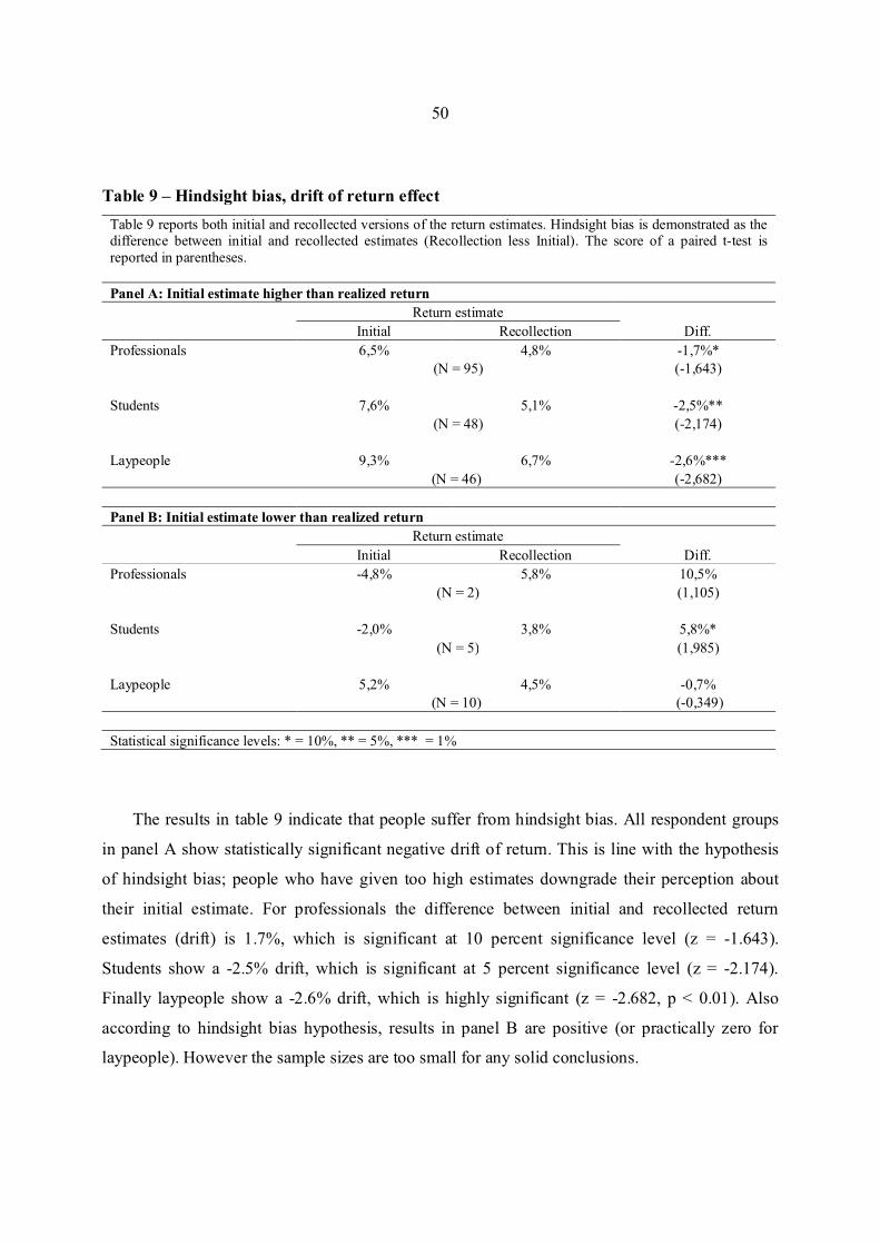
50
Table 9 – Hindsight bias, drift of return effect
Table 9 reports both initial and recollected versions of the return estimates. Hindsight bias is demonstrated as the difference between initial and recollected estimates (Recollection less Initial). The score of a paired t-test is
reported in parentheses.
Panel A: Initial estimate higher than realized return
Return estimate
Initial Recollection Diff.
Professionals 6,5% 4,8% -1,7%*
(N = 95) (-1,643)
Students 7,6% 5,1% -2,5%**
(N = 48) (-2,174)
Laypeople 9,3% 6,7% -2,6%***
(N = 46) (-2,682)
Panel B: Initial estimate lower than realized return
Return estimate
Initial Recollection Diff.
Professionals -4,8% 5,8% 10,5%
(N = 2) (1,105)
Students -2,0% 3,8% 5,8%*
(N = 5) (1,985)
Laypeople 5,2% 4,5% -0,7%
(N = 10) (-0,349)
Statistical significance levels: * = 10%, ** = 5%, *** = 1%
The results in table 9 indicate that people suffer from hindsight bias. All respondent groups
in panel A show statistically significant negative drift of return. This is line with the hypothesis
of hindsight bias; people who have given too high estimates downgrade their perception about
their initial estimate. For professionals the difference between initial and recollected return
estimates (drift) is 1.7%, which is significant at 10 percent significance level (z = -1.643).
Students show a -2.5% drift, which is significant at 5 percent significance level (z = -2.174).
Finally laypeople show a -2.6% drift, which is highly significant (z = -2.682, p < 0.01). Also
according to hindsight bias hypothesis, results in panel B are positive (or practically zero for
laypeople). However the sample sizes are too small for any solid conclusions.
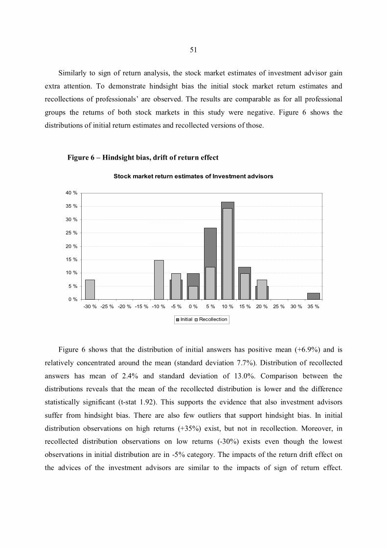
51
Similarly to sign of return analysis, the stock market estimates of investment advisor gain
extra attention. To demonstrate hindsight bias the initial stock market return estimates and
recollections of professionals’ are observed. The results are comparable as for all professional
groups the returns of both stock markets in this study were negative. Figure 6 shows the
distributions of initial return estimates and recollected versions of those.
Figure 6 – Hindsight bias, drift of return effect
Stock market return estimates of Investm ent advisors
0 %
5 %
10 %
15 %
20 %
25 %
30 %
35 %
40 %
-30 % -25 % -20 % -15 % -10 % -5 % 0 % 5 % 10 % 15 % 20 % 25 % 30 % 35 %
Initial Recollection
Figure 6 shows that the distribution of initial answers has positive mean (+6.9%) and is
relatively concentrated around the mean (standard deviation 7.7%). Distribution of recollected
answers has mean of 2.4% and standard deviation of 13.0%. Comparison between the
distributions reveals that the mean of the recollected distribution is lower and the difference
statistically significant (t-stat 1.92). This supports the evidence that also investment advisors
suffer from hindsight bias. There are also few outliers that support hindsight bias. In initial
distribution observations on high returns (+35%) exist, but not in recollection. Moreover, in
recollected distribution observations on low returns (-30%) exists even though the lowest
observations in initial distribution are in -5% category. The impacts of the return drift effect on
the advices of the investment advisors are similar to the impacts of sign of return effect.

52
Investment advisors’ false perceptions of stock market estimation abilities may cause their clients
to take too large risks.
4.1.4. Strength of view
Another way to observe hindsight bias is to study how learning the outcome affects the
perceived certainty in an estimation task. In the framework of this study this is done by asking the
respondents to classify their initial confidence in selecting the better performing asset at phase 1
and also recollecting their initial level of confidence at phase 2. The change between the initial
and recollected confidence is studied. To demonstrate hindsight bias the sample is divided into
two groups; the ones who believe they answered correctly and the ones who believe they
answered incorrectly. According to hindsight bias people who believe they answered correctly
may overestimate the initial certainty and people who believe they answered incorrectly may
underestimate it.
Table 10 presents initial and recollected average strength of view scores for each respondent
group. The difference between panels A and B is that in panel A the sample is limited to answers
where the respondent believed he/she had answered correctly whereas in panel B the sample is
limited to answers where the respondent believed he/she had answered incorrectly. As described
the logic in this is that the recollection may be affected by the realization of the result. The reason
for using the believed answers is to eliminate the effect of falsely remembering own selection.

53
Table 10 – Hindsight bias, strength of view effect
Table 10 reports both initial and recollected versions of the strength of view scores. Hindsight bias is measured as the difference between initial and recollected estimates (Recollection less Initial). The score of a paired t-test is
reported in parentheses. The sample is divided on two panels, A and B. Panel A includes the answers in which
case the respondent believes the answer to be correct. Panel B includes the answers in which case the respondent believes the answer to be correct. The reason for the separation is in the hypothesized direction of effect.
Panel A: Asset selection believed correct
Strength of view
Initial Recollection Diff.
Professionals 2,50 2,56 0,06
(N = 90) (0,52)
Students 2,95 2,77 -0,18
(N = 56) (-1,15)
Laypeople 2,11 2,13 0,02
(N = 47) (0,12)
Panel B: Asset selection believed incorrect
Strength of view
Initial Recollection Diff.
Professionals 2,34 2,11 -0,23*
(N = 47) (-1,80)
Students 2,55 2,26 -0,29**
(N = 42) (-2,14)
Laypeople 2,39 1,79 -0,61***
(N = 38) (-4,07)
Statistical significance levels: * = 10%, ** = 5%, *** = 1%
As can be seen from Panel A people who find their initial selection to be correct do not show
a clear tendency to overestimate the initial certainty. The results in Panel A are controversial; for
professional and laypeople samples the recollected average strength of view is higher than the
initial but for student sample it is lower than the initial. All of the differences are relatively close
to zero and insignificant. Thus no strong conclusions can be made based on this sample. The
evidence does not support the hypothesis that people who find themselves succeeding in a task
increase their belief about their initial confidence in succeeding.
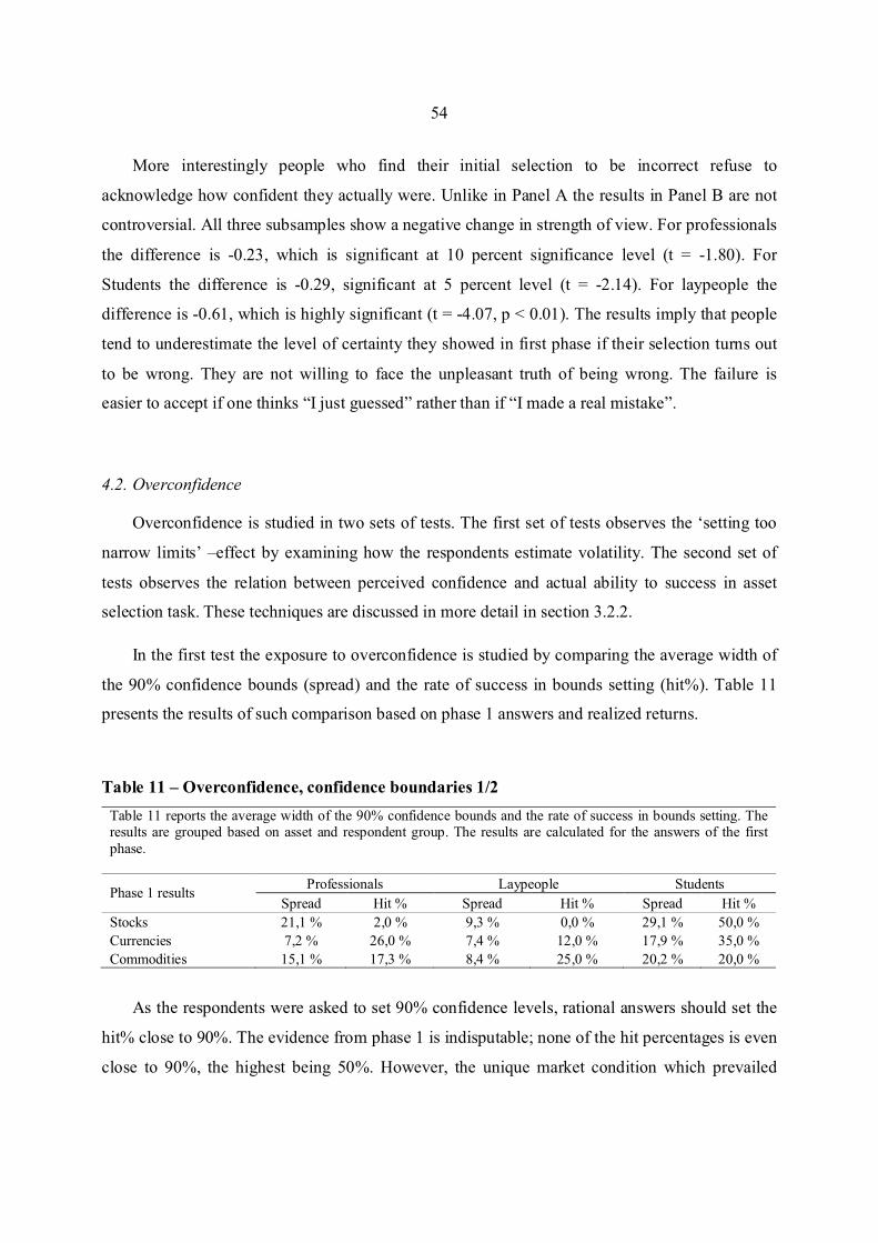
54
More interestingly people who find their initial selection to be incorrect refuse to
acknowledge how confident they actually were. Unlike in Panel A the results in Panel B are not
controversial. All three subsamples show a negative change in strength of view. For professionals
the difference is -0.23, which is significant at 10 percent significance level (t = -1.80). For
Students the difference is -0.29, significant at 5 percent level (t = -2.14). For laypeople the
difference is -0.61, which is highly significant (t = -4.07, p < 0.01). The results imply that people
tend to underestimate the level of certainty they showed in first phase if their selection turns out
to be wrong. They are not willing to face the unpleasant truth of being wrong. The failure is
easier to accept if one thinks “I just guessed” rather than if “I made a real mistake”.
4.2. Overconfidence
Overconfidence is studied in two sets of tests. The first set of tests observes the ‘setting too
narrow limits’ –effect by examining how the respondents estimate volatility. The second set of
tests observes the relation between perceived confidence and actual ability to success in asset
selection task. These techniques are discussed in more detail in section 3.2.2.
In the first test the exposure to overconfidence is studied by comparing the average width of
the 90% confidence bounds (spread) and the rate of success in bounds setting (hit%). Table 11
presents the results of such comparison based on phase 1 answers and realized returns.
Table 11 – Overconfidence, confidence boundaries 1/2
Table 11 reports the average width of the 90% confidence bounds and the rate of success in bounds setting. The results are grouped based on asset and respondent group. The results are calculated for the answers of the first
phase.
Phase 1 results Professionals Laypeople Students
Spread Hit % Spread Hit % Spread Hit %
Stocks 21,1 % 2,0 % 9,3 % 0,0 % 29,1 % 50,0 %
Currencies 7,2 % 26,0 % 7,4 % 12,0 % 17,9 % 35,0 %
Commodities 15,1 % 17,3 % 8,4 % 25,0 % 20,2 % 20,0 %
As the respondents were asked to set 90% confidence levels, rational answers should set the
hit% close to 90%. The evidence from phase 1 is indisputable; none of the hit percentages is even
close to 90%, the highest being 50%. However, the unique market condition which prevailed
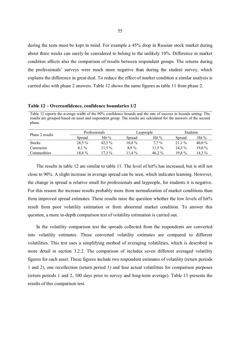
55
during the tests must be kept in mind. For example a 45% drop in Russian stock market during
about three weeks can surely be considered to belong to the unlikely 10%. Difference in market
condition affects also the comparison of results between respondent groups. The returns during
the professionals’ surveys were much more negative than during the student survey, which
explains the difference in great deal. To reduce the effect of market condition a similar analysis is
carried also with phase 2 answers. Table 12 shows the same figures as table 11 from phase 2.
Table 12 – Overconfidence, confidence boundaries 1/2
Table 12 reports the average width of the 90% confidence bounds and the rate of success in bounds setting. The results are grouped based on asset and respondent group. The results are calculated for the answers of the second
phase.
Phase 2 results Professionals Laypeople Students
Spread Hit % Spread Hit % Spread Hit %
Stocks 28,5 % 42,3 % 10,8 % 7,7 % 21,1 % 40,0 %
Currencies 8,1 % 11,5 % 8,9 % 11,5 % 14,3 % 19,0 %
Commodities 18,8 % 17,3 % 11,4 % 46,2 % 19,8 % 14,3 %
The results in table 12 are similar to table 11. The level of hit% has increased, but is still not
close to 90%. A slight increase in average spread can be seen, which indicates learning. However,
the change in spread is relative small for professionals and laypeople, for students it is negative.
For this reason the increase results probably more from normalization of market conditions than
from improved spread estimates. These results raise the question whether the low levels of hit%
result from poor volatility estimation or from abnormal market condition. To answer this
question, a more in-depth comparison test of volatility estimation is carried out.
In the volatility comparison test the spreads collected from the respondents are converted
into volatility estimates. These converted volatility estimates are compared to different
volatilities. This test uses a simplifying method of averaging volatilities, which is described in
more detail in section 3.2.2. The comparison of includes seven different averaged volatility
figures for each asset. These figures include two respondent estimates of volatility (return periods
1 and 2), one recollection (return period 1) and four actual volatilities for comparison purposes
(return periods 1 and 2, 100 days prior to survey and long-term average). Table 13 presents the
results of this comparison test.
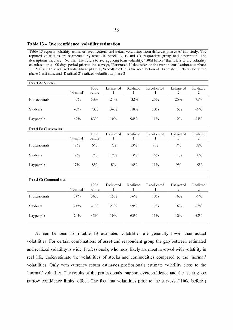
56
Table 13 – Overconfidence, volatility estimation
Table 13 reports volatility estimates, recollections and actual volatilities from different phases of this study. The reported volatilities are segmented by asset (in panels A, B and C), respondent group and description. The
descriptions used are: ‘Normal’ that refers to average long term volatility, ‘100d before’ that refers to the volatility
calculated on a 100 days period prior to the surveys, ‘Estimated 1’ that refers to the respondents’ estimate at phase
1, ‘Realized 1’ is realized volatility at phase 1, ‘Recollected 1’ is the recollection of ‘Estimate 1’, ‘Estimate 2’ the phase 2 estimate, and ‘Realized 2’ realized volatility at phase 2
Panel A: Stocks
‘Normal’ 100d
before Estimated
1 Realized
1 Recollected
1 Estimated
2 Realized
2
Professionals 47% 53% 21% 132% 25% 25% 75%
Students 47% 73% 34% 118% 20% 15% 69%
Laypeople 47% 83% 10% 98% 11% 12% 61%
Panel B: Currencies
‘Normal’ 100d
before Estimated
1 Realized
1 Recollected
1 Estimated
2 Realized
2
Professionals 7% 6% 7% 13% 9% 7% 18%
Students 7% 7% 19% 13% 15% 11% 18%
Laypeople 7% 8% 8% 16% 11% 9% 19%
Panel C: Commodities
‘Normal’
100d
before
Estimated
1
Realized
1
Recollected
1
Estimated
2
Realized
2
Professionals 24% 36% 15% 56% 18% 16% 59%
Students 24% 41% 23% 59% 17% 16% 63%
Laypeople 24% 43% 10% 62% 11% 12% 62%
As can be seen from table 13 estimated volatilities are generally lower than actual
volatilities. For certain combinations of asset and respondent group the gap between estimated
and realized volatility is wide. Professionals, who most likely are most involved with volatility in
real life, underestimate the volatilities of stocks and commodities compared to the ‘normal’
volatilities. Only with currency return estimates professionals estimate volatility close to the
‘normal’ volatility. The results of the professionals’ support overconfidence and the ‘setting too
narrow confidence limits’ effect. The fact that volatilities prior to the surveys (‘100d before’)
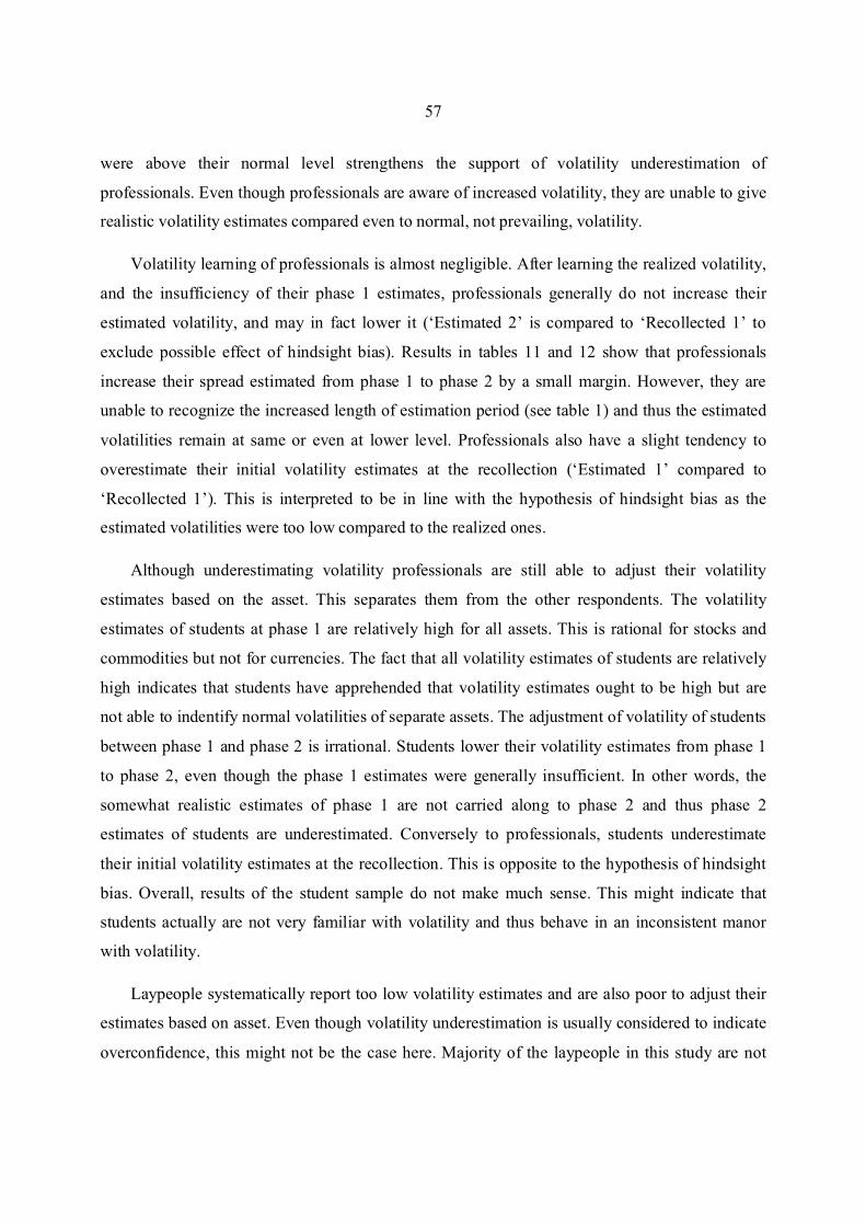
57
were above their normal level strengthens the support of volatility underestimation of
professionals. Even though professionals are aware of increased volatility, they are unable to give
realistic volatility estimates compared even to normal, not prevailing, volatility.
Volatility learning of professionals is almost negligible. After learning the realized volatility,
and the insufficiency of their phase 1 estimates, professionals generally do not increase their
estimated volatility, and may in fact lower it (‘Estimated 2’ is compared to ‘Recollected 1’ to
exclude possible effect of hindsight bias). Results in tables 11 and 12 show that professionals
increase their spread estimated from phase 1 to phase 2 by a small margin. However, they are
unable to recognize the increased length of estimation period (see table 1) and thus the estimated
volatilities remain at same or even at lower level. Professionals also have a slight tendency to
overestimate their initial volatility estimates at the recollection (‘Estimated 1’ compared to
‘Recollected 1’). This is interpreted to be in line with the hypothesis of hindsight bias as the
estimated volatilities were too low compared to the realized ones.
Although underestimating volatility professionals are still able to adjust their volatility
estimates based on the asset. This separates them from the other respondents. The volatility
estimates of students at phase 1 are relatively high for all assets. This is rational for stocks and
commodities but not for currencies. The fact that all volatility estimates of students are relatively
high indicates that students have apprehended that volatility estimates ought to be high but are
not able to indentify normal volatilities of separate assets. The adjustment of volatility of students
between phase 1 and phase 2 is irrational. Students lower their volatility estimates from phase 1
to phase 2, even though the phase 1 estimates were generally insufficient. In other words, the
somewhat realistic estimates of phase 1 are not carried along to phase 2 and thus phase 2
estimates of students are underestimated. Conversely to professionals, students underestimate
their initial volatility estimates at the recollection. This is opposite to the hypothesis of hindsight
bias. Overall, results of the student sample do not make much sense. This might indicate that
students actually are not very familiar with volatility and thus behave in an inconsistent manor
with volatility.
Laypeople systematically report too low volatility estimates and are also poor to adjust their
estimates based on asset. Even though volatility underestimation is usually considered to indicate
overconfidence, this might not be the case here. Majority of the laypeople in this study are not
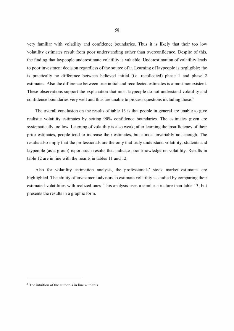
58
very familiar with volatility and confidence boundaries. Thus it is likely that their too low
volatility estimates result from poor understanding rather than overconfidence. Despite of this,
the finding that laypeople underestimate volatility is valuable. Underestimation of volatility leads
to poor investment decision regardless of the source of it. Learning of laypeople is negligible; the
is practically no difference between believed initial (i.e. recollected) phase 1 and phase 2
estimates. Also the difference between true initial and recollected estimates is almost nonexistent.
These observations support the explanation that most laypeople do not understand volatility and
confidence boundaries very well and thus are unable to process questions including those.5
The overall conclusion on the results of table 13 is that people in general are unable to give
realistic volatility estimates by setting 90% confidence boundaries. The estimates given are
systematically too low. Learning of volatility is also weak; after learning the insufficiency of their
prior estimates, people tend to increase their estimates, but almost invariably not enough. The
results also imply that the professionals are the only that truly understand volatility; students and
laypeople (as a group) report such results that indicate poor knowledge on volatility. Results in
table 12 are in line with the results in tables 11 and 12.
Also for volatility estimation analysis, the professionals’ stock market estimates are
highlighted. The ability of investment advisors to estimate volatility is studied by comparing their
estimated volatilities with realized ones. This analysis uses a similar structure than table 13, but
presents the results in a graphic form.
5 The intuition of the author is in line with this.

59
Figure 7 – Overconfidence, volatility estimation
47 %53 %
21 %
132 %
25 % 25 %
75 %
0 %
20 %
40 %
60 %
80 %
100 %
120 %
140 %
'Normal' 100d before Estimated 1 Realized 1 Recollected 1 Estimated 2 Realized 2
Vo
lati
lity
Professionals' stock m arket volatility estim ation
Results in figure 7 are in line with the results in table 13; investment advisors underestimate
volatility by a wide margin. The estimated volatility for return period 1 is significantly lower than
‘normal’ or prevailing (100d before) volatility. Volatility learning is also poor; estimated
volatility for return period 2 is equal to the respondents’ perceived period 1 volatility (i.e.
recollected). The difference between the initial and recollected volatility is slightly positive,
which is line with the hypothesis of hindsight bias.
W hen interpreting the results of figure 7, it should be noticed that the ‘normal’ refers to the
average volatilities of Brazilian and Russian stock market. The ‘normal’ annual long term
volatility of U.S. stock market is significantly lower, about 15%6. It might be that investment
advisors are simply unable to devolve the information that emerging markets are riskier than
developed markets, which they surely agree on, to their volatility estimates. Even so, the finding
that investment advisors underestimate volatility and are unable to learn is valuable. The fact that
it holds also for stock market estimates affects the quality of investment advisors’ advices to their
customers. As even the professionals are not able to assess risk in proper way, it is almost
impossible for the clients who have faith in the abilities of their advisors. The fact that investment
advisor are unaware of their tendency to underestimate volatility prevents them from controlling
6 Dow Jones Industrials Average Price Index between 2.1.1951 and 6.8.2009
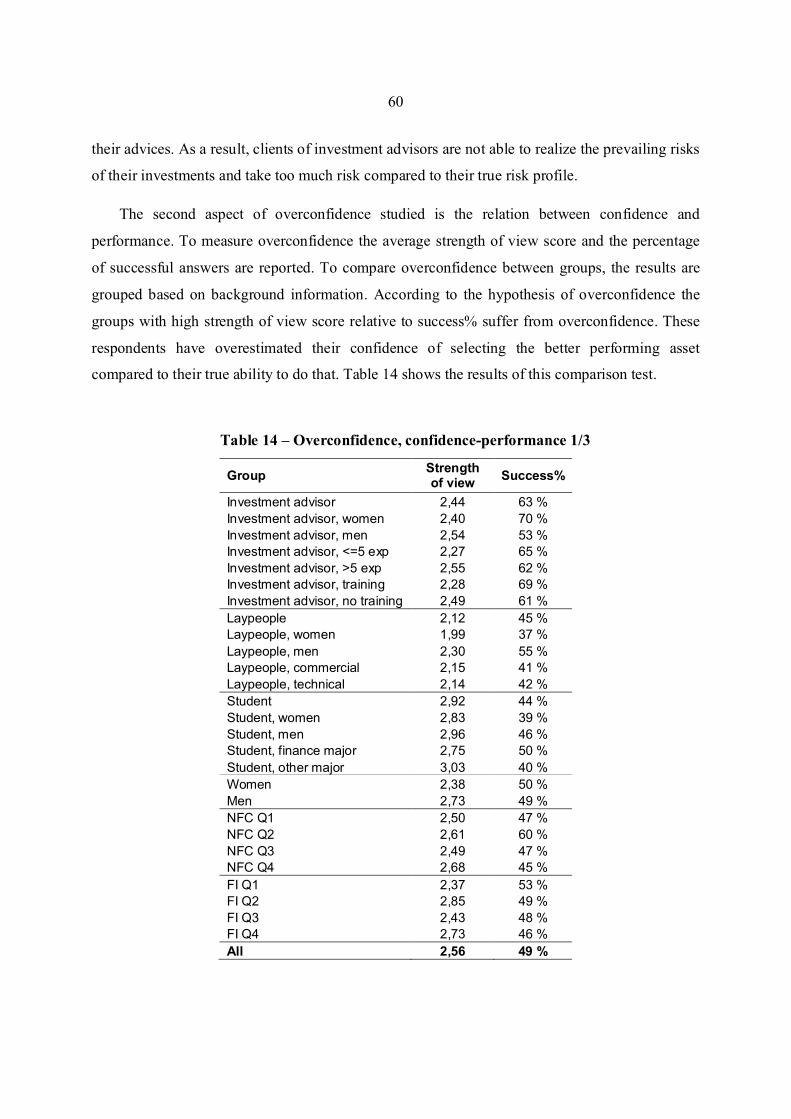
60
their advices. As a result, clients of investment advisors are not able to realize the prevailing risks
of their investments and take too much risk compared to their true risk profile.
The second aspect of overconfidence studied is the relation between confidence and
performance. To measure overconfidence the average strength of view score and the percentage
of successful answers are reported. To compare overconfidence between groups, the results are
grouped based on background information. According to the hypothesis of overconfidence the
groups with high strength of view score relative to success% suffer from overconfidence. These
respondents have overestimated their confidence of selecting the better performing asset
compared to their true ability to do that. Table 14 shows the results of this comparison test.
Table 14 – Overconfidence, confidence-performance 1/3
Group Strength of view
Success%
Investment advisor 2,44 63 %
Investment advisor, women 2,40 70 %
Investment advisor, men 2,54 53 %
Investment advisor, <=5 exp 2,27 65 %
Investment advisor, >5 exp 2,55 62 %
Investment advisor, training 2,28 69 %
Investment advisor, no training 2,49 61 %
Laypeople 2,12 45 %
Laypeople, women 1,99 37 %
Laypeople, men 2,30 55 %
Laypeople, commercial 2,15 41 %
Laypeople, technical 2,14 42 %
Student 2,92 44 %
Student, women 2,83 39 %
Student, men 2,96 46 %
Student, finance major 2,75 50 %
Student, other major 3,03 40 %
W omen 2,38 50 %
Men 2,73 49 %
NFC Q1 2,50 47 %
NFC Q2 2,61 60 %
NFC Q3 2,49 47 %
NFC Q4 2,68 45 %
FI Q1 2,37 53 %
FI Q2 2,85 49 %
FI Q3 2,43 48 %
FI Q4 2,73 46 %
All 2,56 49 %
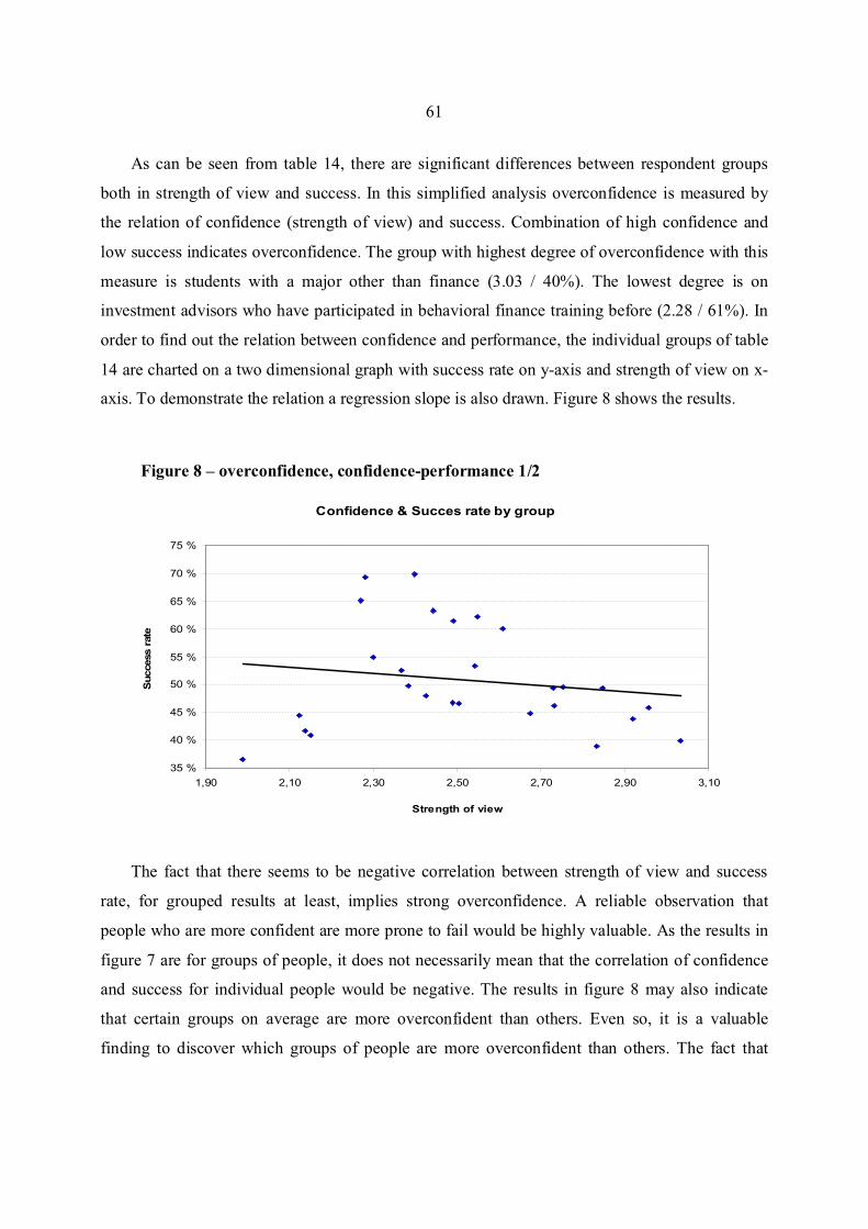
61
As can be seen from table 14, there are significant differences between respondent groups
both in strength of view and success. In this simplified analysis overconfidence is measured by
the relation of confidence (strength of view) and success. Combination of high confidence and
low success indicates overconfidence. The group with highest degree of overconfidence with this
measure is students with a major other than finance (3.03 / 40%). The lowest degree is on
investment advisors who have participated in behavioral finance training before (2.28 / 61%). In
order to find out the relation between confidence and performance, the individual groups of table
14 are charted on a two dimensional graph with success rate on y-axis and strength of view on x-
axis. To demonstrate the relation a regression slope is also drawn. Figure 8 shows the results.
Figure 8 – overconfidence, confidence-performance 1/2
Confidence & Succes rate by group
35 %
40 %
45 %
50 %
55 %
60 %
65 %
70 %
75 %
1,90 2,10 2,30 2,50 2,70 2,90 3,10
Strength of view
Success r
ate
The fact that there seems to be negative correlation between strength of view and success
rate, for grouped results at least, implies strong overconfidence. A reliable observation that
people who are more confident are more prone to fail would be highly valuable. As the results in
figure 7 are for groups of people, it does not necessarily mean that the correlation of confidence
and success for individual people would be negative. The results in figure 8 may also indicate
that certain groups on average are more overconfident than others. Even so, it is a valuable
finding to discover which groups of people are more overconfident than others. The fact that
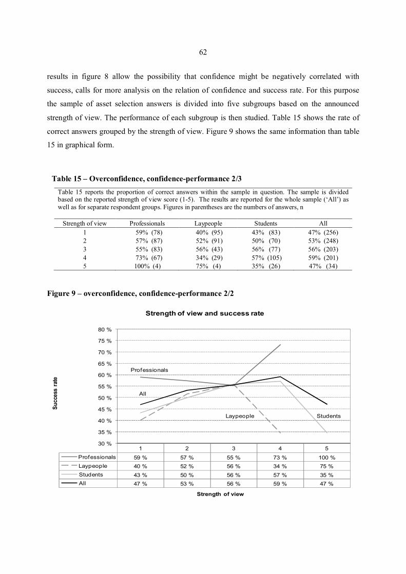
62
results in figure 8 allow the possibility that confidence might be negatively correlated with
success, calls for more analysis on the relation of confidence and success rate. For this purpose
the sample of asset selection answers is divided into five subgroups based on the announced
strength of view. The performance of each subgroup is then studied. Table 15 shows the rate of
correct answers grouped by the strength of view. Figure 9 shows the same information than table
15 in graphical form.
Table 15 – Overconfidence, confidence-performance 2/3
Table 15 reports the proportion of correct answers within the sample in question. The sample is divided based on the reported strength of view score (1-5). The results are reported for the whole sample (‘All’) as
well as for separate respondent groups. Figures in parentheses are the numbers of answers, n
Strength of view Professionals Laypeople Students All
1 59% (78) 40% (95) 43% (83) 47% (256)
2 57% (87) 52% (91) 50% (70) 53% (248)
3 55% (83) 56% (43) 56% (77) 56% (203)
4 73% (67) 34% (29) 57% (105) 59% (201)
5 100% (4) 75% (4) 35% (26) 47% (34)
Figure 9 – overconfidence, confidence-performance 2/2
1 2 3 4 5
Professionals 59 % 57 % 55 % 73 % 100 %
Laypeople 40 % 52 % 56 % 34 % 75 %
Students 43 % 50 % 56 % 57 % 35 %
All 47 % 53 % 56 % 59 % 47 %
Professionals
Laypeople Students
All
30 %
35 %
40 %
45 %
50 %
55 %
60 %
65 %
70 %
75 %
80 %
Su
cce
ss r
ate
Strength of view
Strength of view and success rate
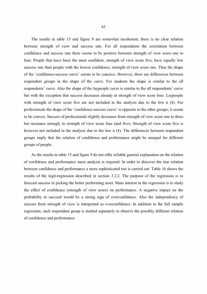
63
The results in table 15 and figure 9 are somewhat incoherent; there is no clear relation
between strength of view and success rate. For all respondents the correlation between
confidence and success rate there seems to be positive between strength of view score one to
four. People that have been the most confident, strength of view score five, have equally low
success rate than people with the lowest confidence, strength of view score one. Thus the shape
of the ‘confidence-success curve’ seems to be concave. However, there are differences between
respondent groups in the shape of the curve. For students the shape is similar to the all
respondents’ curve. Also the shape of the laypeople curve is similar to the all respondents’ curve
but with the exception that success decreases already at strength of view score four. Laypeople
with strength of view score five are not included in the analysis due to the low n (4). For
professionals the shape of the ‘confidence-success curve’ is opposite to the other groups; it seems
to be convex. Success of professionals slightly decreases from strength of view score one to three
but increases strongly in strength of view score four (and five). Strength of view score five is
however not included in the analysis due to the low n (4). The differences between respondent
groups imply that the relation of confidence and performance might be unequal for different
groups of people.
As the results in table 15 and figure 9 do not offer reliable general explanation on the relation
of confidence and performance more analysis is required. In order to discover the true relation
between confidence and performance a more sophisticated test is carried out. Table 16 shows the
results of the logit-regression described in section 3.2.2. The purpose of the regression is to
forecast success in picking the better performing asset. Main interest in the regression is to study
the effect of confidence (strength of view score) on performance. A negative impact on the
probability to succeed would be a strong sign of overconfidence. Also the independency of
success from strength of view is interpreted as overconfidence. In addition to the full sample
regression, each respondent group is studied separately to observe the possibly different relation
of confidence and performance.
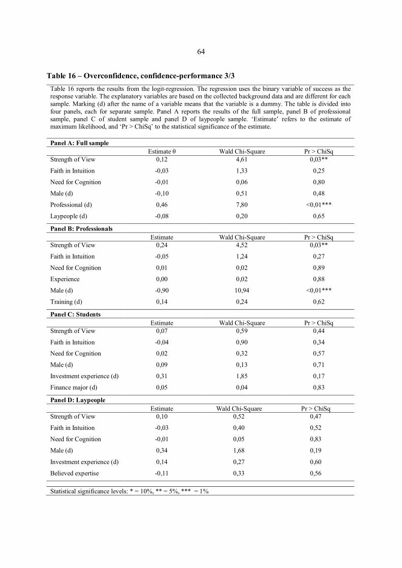
64
Table 16 – Overconfidence, confidence-performance 3/3
Table 16 reports the results from the logit-regression. The regression uses the binary variable of success as the response variable. The explanatory variables are based on the collected background data and are different for each
sample. Marking (d) after the name of a variable means that the variable is a dummy. The table is divided into
four panels, each for separate sample. Panel A reports the results of the full sample, panel B of professional
sample, panel C of student sample and panel D of laypeople sample. ‘Estimate’ refers to the estimate of maximum likelihood, and ‘Pr > ChiSq’ to the statistical significance of the estimate.
Panel A: Full sample
Estimate � W ald Chi-Square Pr > ChiSq
Strength of View 0,12 4,61 0,03**
Faith in Intuition -0,03 1,33 0,25
Need for Cognition -0,01 0,06 0,80
Male (d) -0,10 0,51 0,48
Professional (d) 0,46 7,80 <0,01***
Laypeople (d) -0,08 0,20 0,65
Panel B: Professionals
Estimate W ald Chi-Square Pr > ChiSq
Strength of View 0,24 4,52 0,03**
Faith in Intuition -0,05 1,24 0,27
Need for Cognition 0,01 0,02 0,89
Experience 0,00 0,02 0,88
Male (d) -0,90 10,94 <0,01***
Training (d) 0,14 0,24 0,62
Panel C: Students
Estimate W ald Chi-Square Pr > ChiSq
Strength of View 0,07 0,59 0,44
Faith in Intuition -0,04 0,90 0,34
Need for Cognition 0,02 0,32 0,57
Male (d) 0,09 0,13 0,71
Investment experience (d) 0,31 1,85 0,17
Finance major (d) 0,05 0,04 0,83
Panel D: Laypeople
Estimate W ald Chi-Square Pr > ChiSq
Strength of View 0,10 0,52 0,47
Faith in Intuition -0,03 0,40 0,52
Need for Cognition -0,01 0,05 0,83
Male (d) 0,34 1,68 0,19
Investment experience (d) 0,14 0,27 0,60
Believed expertise -0,11 0,33 0,56
Statistical significance levels: * = 10%, ** = 5%, *** = 1%
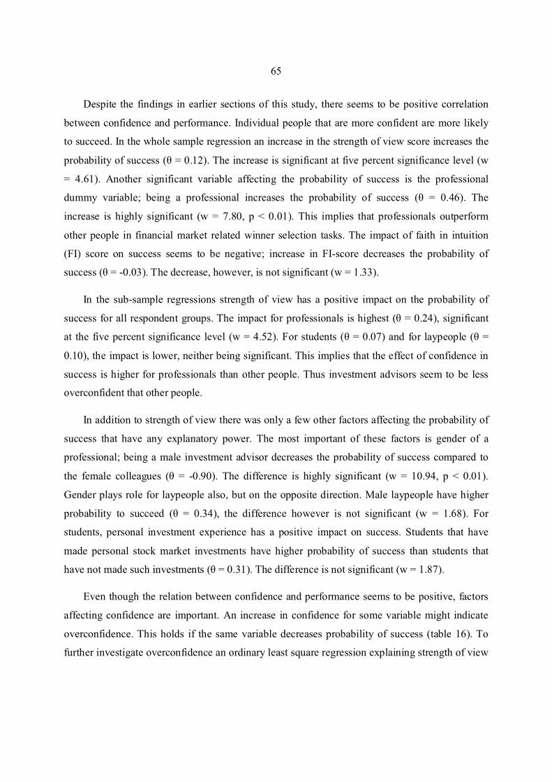
65
Despite the findings in earlier sections of this study, there seems to be positive correlation
between confidence and performance. Individual people that are more confident are more likely
to succeed. In the whole sample regression an increase in the strength of view score increases the
probability of success (� = 0.12). The increase is significant at five percent significance level (w
= 4.61). Another significant variable affecting the probability of success is the professional
dummy variable; being a professional increases the probability of success (� = 0.46). The
increase is highly significant (w = 7.80, p < 0.01). This implies that professionals outperform
other people in financial market related winner selection tasks. The impact of faith in intuition
(FI) score on success seems to be negative; increase in FI-score decreases the probability of
success (� = -0.03). The decrease, however, is not significant (w = 1.33).
In the sub-sample regressions strength of view has a positive impact on the probability of
success for all respondent groups. The impact for professionals is highest (� = 0.24), significant
at the five percent significance level (w = 4.52). For students (� = 0.07) and for laypeople (� =
0.10), the impact is lower, neither being significant. This implies that the effect of confidence in
success is higher for professionals than other people. Thus investment advisors seem to be less
overconfident that other people.
In addition to strength of view there was only a few other factors affecting the probability of
success that have any explanatory power. The most important of these factors is gender of a
professional; being a male investment advisor decreases the probability of success compared to
the female colleagues (� = -0.90). The difference is highly significant (w = 10.94, p < 0.01).
Gender plays role for laypeople also, but on the opposite direction. Male laypeople have higher
probability to succeed (� = 0.34), the difference however is not significant (w = 1.68). For
students, personal investment experience has a positive impact on success. Students that have
made personal stock market investments have higher probability of success than students that
have not made such investments (� = 0.31). The difference is not significant (w = 1.87).
Even though the relation between confidence and performance seems to be positive, factors
affecting confidence are important. An increase in confidence for some variable might indicate
overconfidence. This holds if the same variable decreases probability of success (table 16). To
further investigate overconfidence an ordinary least square regression explaining strength of view
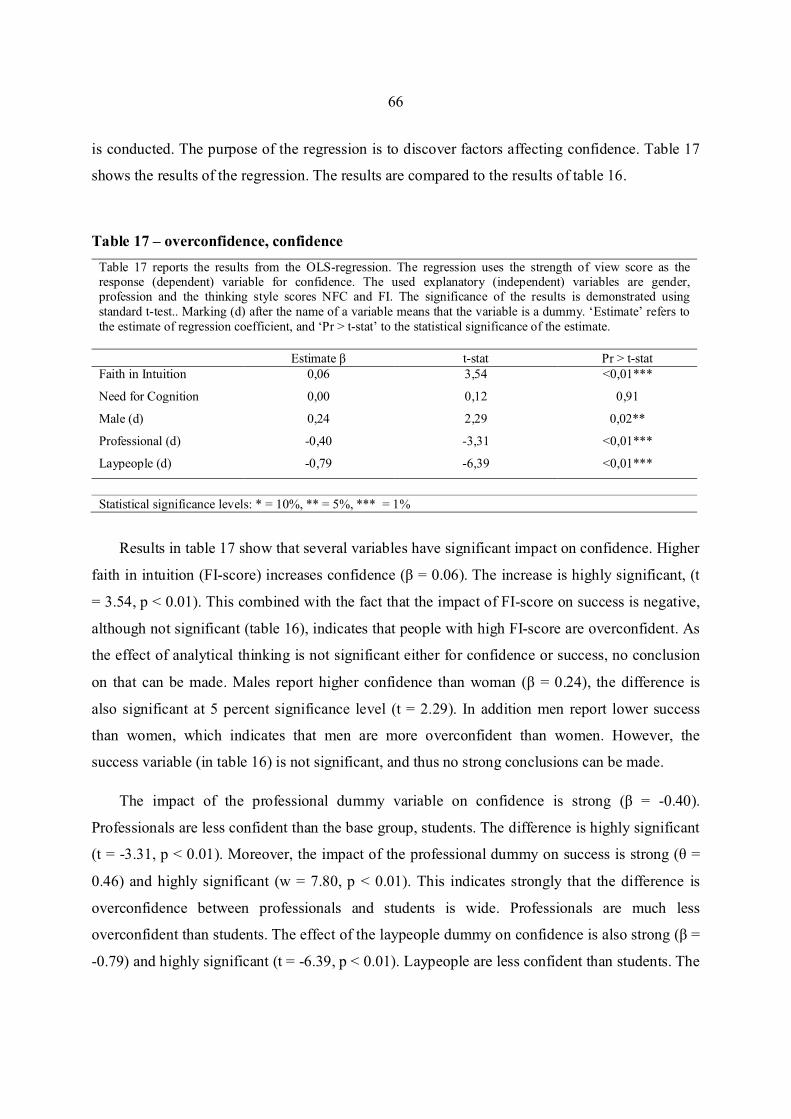
66
is conducted. The purpose of the regression is to discover factors affecting confidence. Table 17
shows the results of the regression. The results are compared to the results of table 16.
Table 17 – overconfidence, confidence
Table 17 reports the results from the OLS-regression. The regression uses the strength of view score as the response (dependent) variable for confidence. The used explanatory (independent) variables are gender, profession and the thinking style scores NFC and FI. The significance of the results is demonstrated using
standard t-test.. Marking (d) after the name of a variable means that the variable is a dummy. ‘Estimate’ refers to
the estimate of regression coefficient, and ‘Pr > t-stat’ to the statistical significance of the estimate.
Estimate ! t-stat Pr > t-stat
Faith in Intuition 0,06 3,54 <0,01***
Need for Cognition 0,00 0,12 0,91
Male (d) 0,24 2,29 0,02**
Professional (d) -0,40 -3,31 <0,01***
Laypeople (d) -0,79 -6,39 <0,01***
Statistical significance levels: * = 10%, ** = 5%, *** = 1%
Results in table 17 show that several variables have significant impact on confidence. Higher
faith in intuition (FI-score) increases confidence (! = 0.06). The increase is highly significant, (t
= 3.54, p < 0.01). This combined with the fact that the impact of FI-score on success is negative,
although not significant (table 16), indicates that people with high FI-score are overconfident. As
the effect of analytical thinking is not significant either for confidence or success, no conclusion
on that can be made. Males report higher confidence than woman (! = 0.24), the difference is
also significant at 5 percent significance level (t = 2.29). In addition men report lower success
than women, which indicates that men are more overconfident than women. However, the
success variable (in table 16) is not significant, and thus no strong conclusions can be made.
The impact of the professional dummy variable on confidence is strong (! = -0.40).
Professionals are less confident than the base group, students. The difference is highly significant
(t = -3.31, p < 0.01). Moreover, the impact of the professional dummy on success is strong (� =
0.46) and highly significant (w = 7.80, p < 0.01). This indicates strongly that the difference is
overconfidence between professionals and students is wide. Professionals are much less
overconfident than students. The effect of the laypeople dummy on confidence is also strong (! =
-0.79) and highly significant (t = -6.39, p < 0.01). Laypeople are less confident than students. The

67
effect of laypeople dummy on success is slightly negative (� = -0.08), but not significant. Thus
the results indicate that laypeople are less overconfident than students. The difference, however,
is not as significant as between professionals and students.
4.3. Self-attribution bias
Self-attribution bias is studied in two tests. Both tests measure self-attribution bias by the
change in perceived certainty of success between first and second rounds. The difference is in the
determination of success. First test uses individual answers whereas second test uses pooled
answers for a single person. The techniques used are discussed in more detail in section 3.2.3.
The first test bases on an attribution of self-attribution bias according to which people who
believe they have succeeded in a winner selection task attribute themselves on the success. As a
result of this, such people overestimate their own capability and become more confident.
Similarly people who believe they failed in a winner selection task attribute themselves on the
failure and become less confident. To demonstrate self-attribution bias the sample of asset
selection answers of this study is divided into two sub-samples based on the believed correctness.
Self-attribution bias is measured by the change in strength of view score between the rounds.
Table 18 presents the results. To demonstrate the statistical significance a paired t-test is carried.
Table 18 – Self-attribution bias, individual answers test
Table 18 reports both the recollected phase 1 and phase 2 strength of view scores. Self-attribution bias is
measured by the difference between these (Phase 2 less Phase 1). The score of a paired t-test is reported in parentheses. The sample is divided on two panels, A and B. Panel A includes the answers in which case the
respondent believes the answer to be correct. Panel B includes the answers in which case the respondent believes
the answer to be correct. The reason for the separation is in the hypothesized direction of effect.
Panel A: Asset selection believed correct
Strength of view
Phase 1 (recollection) Phase 2 Diff.
Professionals 2,50 2,68 0,18*
(N = 90) (1,666)
Students 2,74 2,80 0,06
(N = 50) (0,401)
Laypeople 2,09 2,14 0,05
(N = 44) (0,443)
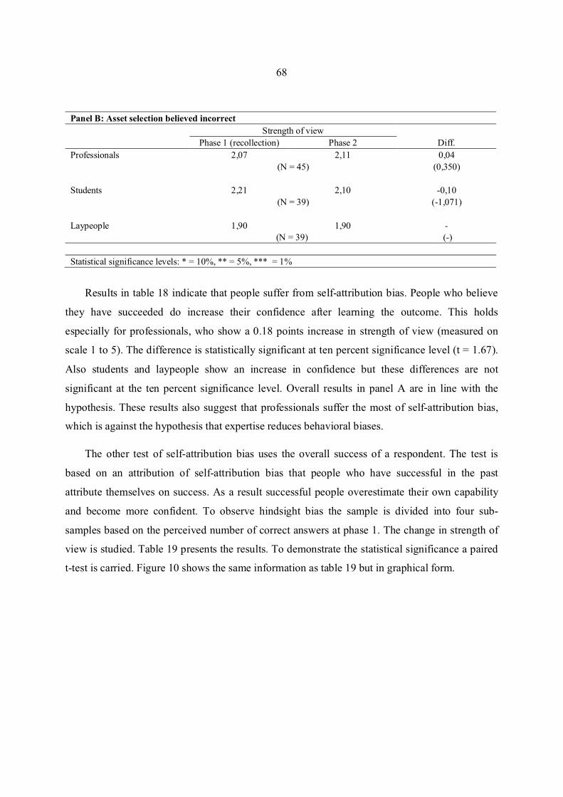
68
Panel B: Asset selection believed incorrect
Strength of view
Phase 1 (recollection) Phase 2 Diff.
Professionals 2,07 2,11 0,04
(N = 45) (0,350)
Students 2,21 2,10 -0,10
(N = 39) (-1,071)
Laypeople 1,90 1,90 -
(N = 39) (-)
Statistical significance levels: * = 10%, ** = 5%, *** = 1%
Results in table 18 indicate that people suffer from self-attribution bias. People who believe
they have succeeded do increase their confidence after learning the outcome. This holds
especially for professionals, who show a 0.18 points increase in strength of view (measured on
scale 1 to 5). The difference is statistically significant at ten percent significance level (t = 1.67).
Also students and laypeople show an increase in confidence but these differences are not
significant at the ten percent significance level. Overall results in panel A are in line with the
hypothesis. These results also suggest that professionals suffer the most of self-attribution bias,
which is against the hypothesis that expertise reduces behavioral biases.
The other test of self-attribution bias uses the overall success of a respondent. The test is
based on an attribution of self-attribution bias that people who have successful in the past
attribute themselves on success. As a result successful people overestimate their own capability
and become more confident. To observe hindsight bias the sample is divided into four sub-
samples based on the perceived number of correct answers at phase 1. The change in strength of
view is studied. Table 19 presents the results. To demonstrate the statistical significance a paired
t-test is carried. Figure 10 shows the same information as table 19 but in graphical form.
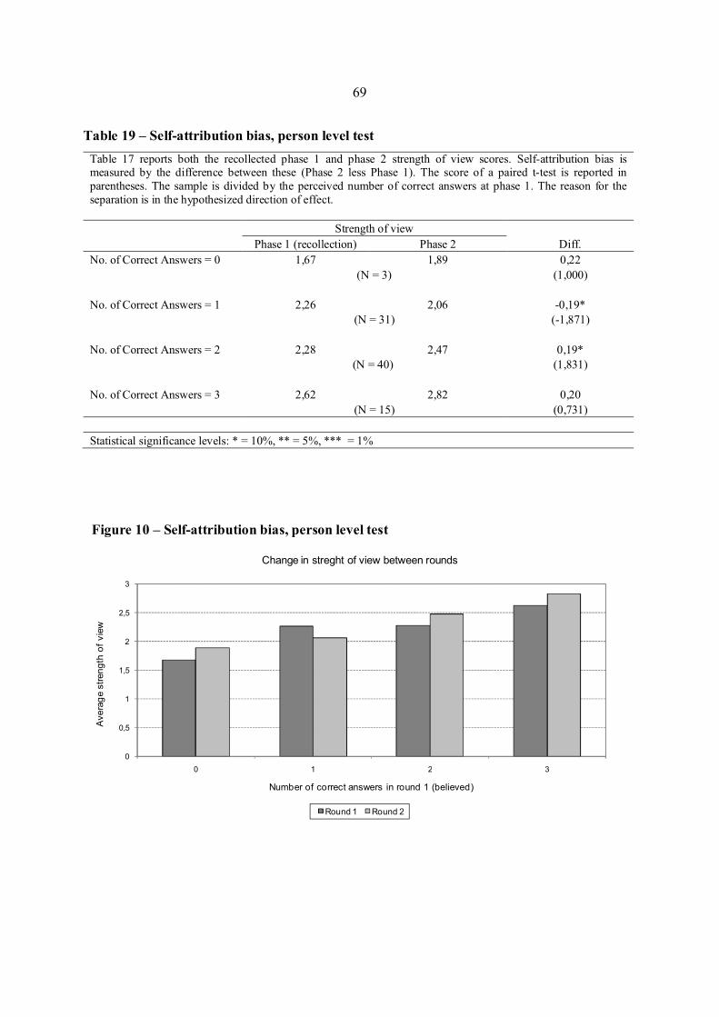
69
Table 19 – Self-attribution bias, person level test
Table 17 reports both the recollected phase 1 and phase 2 strength of view scores. Self-attribution bias is measured by the difference between these (Phase 2 less Phase 1). The score of a paired t-test is reported in
parentheses. The sample is divided by the perceived number of correct answers at phase 1. The reason for the
separation is in the hypothesized direction of effect.
Strength of view
Phase 1 (recollection) Phase 2 Diff.
No. of Correct Answers = 0 1,67 1,89 0,22
(N = 3) (1,000)
No. of Correct Answers = 1 2,26 2,06 -0,19*
(N = 31) (-1,871)
No. of Correct Answers = 2 2,28 2,47 0,19*
(N = 40) (1,831)
No. of Correct Answers = 3 2,62 2,82 0,20
(N = 15) (0,731)
Statistical significance levels: * = 10%, ** = 5%, *** = 1%
Figure 10 – Self-attribution bias, person level test
0
0,5
1
1,5
2
2,5
3
0 1 2 3
Ave
rag
e s
tren
gth
of
vie
w
Number of correct answers in round 1 (believed)
Change in streght of view between rounds
Round 1 Round 2
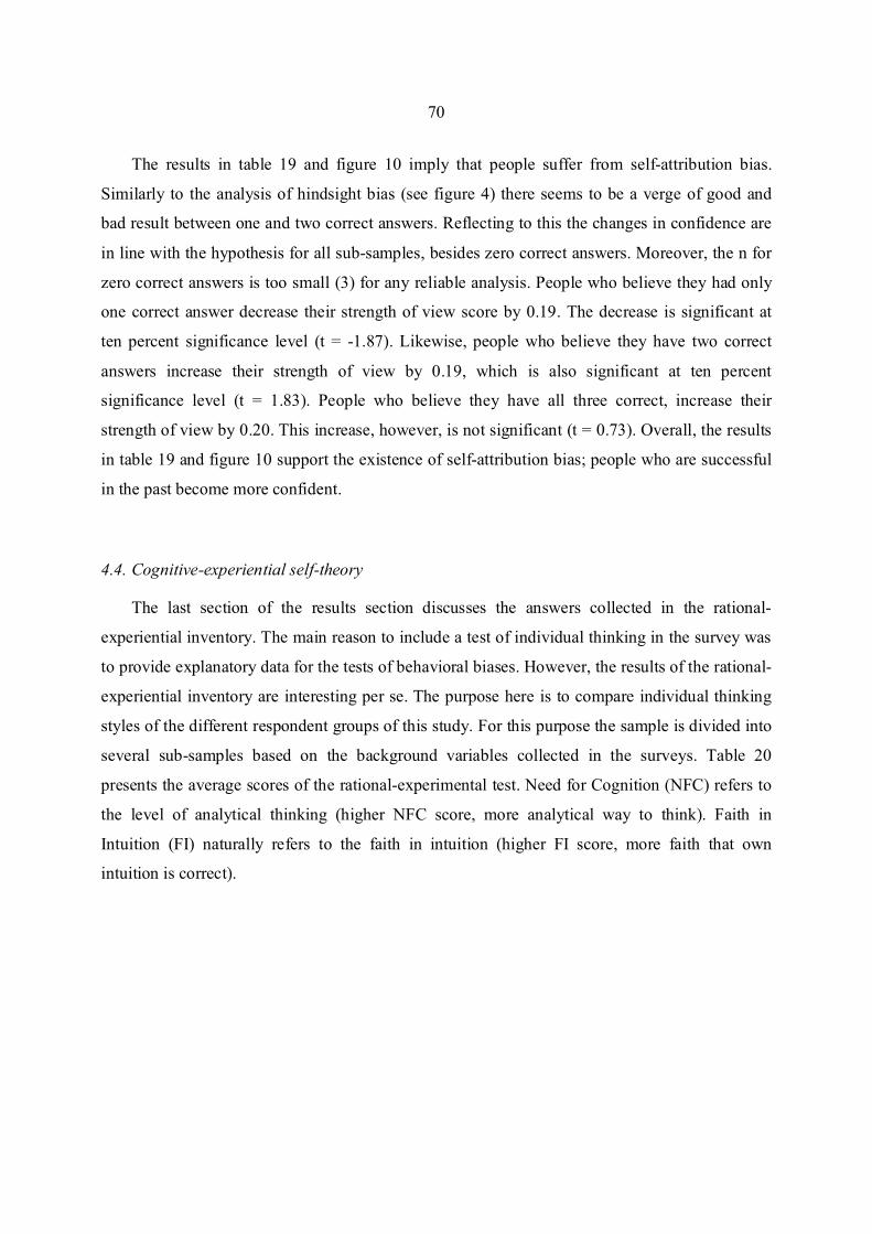
70
The results in table 19 and figure 10 imply that people suffer from self-attribution bias.
Similarly to the analysis of hindsight bias (see figure 4) there seems to be a verge of good and
bad result between one and two correct answers. Reflecting to this the changes in confidence are
in line with the hypothesis for all sub-samples, besides zero correct answers. Moreover, the n for
zero correct answers is too small (3) for any reliable analysis. People who believe they had only
one correct answer decrease their strength of view score by 0.19. The decrease is significant at
ten percent significance level (t = -1.87). Likewise, people who believe they have two correct
answers increase their strength of view by 0.19, which is also significant at ten percent
significance level (t = 1.83). People who believe they have all three correct, increase their
strength of view by 0.20. This increase, however, is not significant (t = 0.73). Overall, the results
in table 19 and figure 10 support the existence of self-attribution bias; people who are successful
in the past become more confident.
4.4. Cognitive-experiential self-theory
The last section of the results section discusses the answers collected in the rational-
experiential inventory. The main reason to include a test of individual thinking in the survey was
to provide explanatory data for the tests of behavioral biases. However, the results of the rational-
experiential inventory are interesting per se. The purpose here is to compare individual thinking
styles of the different respondent groups of this study. For this purpose the sample is divided into
several sub-samples based on the background variables collected in the surveys. Table 20
presents the average scores of the rational-experimental test. Need for Cognition (NFC) refers to
the level of analytical thinking (higher NFC score, more analytical way to think). Faith in
Intuition (FI) naturally refers to the faith in intuition (higher FI score, more faith that own
intuition is correct).
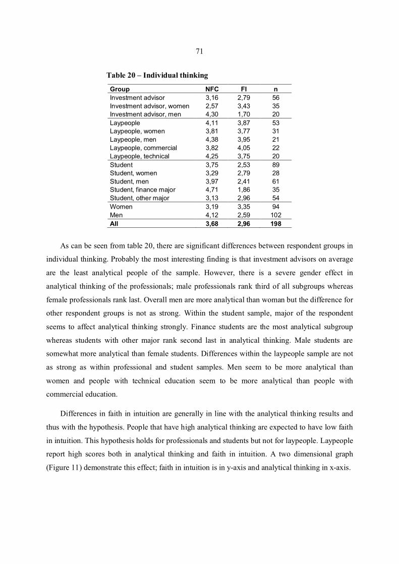
71
Table 20 – Individual thinking
Group NFC FI n
Investment advisor 3,16 2,79 56
Investment advisor, women 2,57 3,43 35
Investment advisor, men 4,30 1,70 20
Laypeople 4,11 3,87 53
Laypeople, women 3,81 3,77 31
Laypeople, men 4,38 3,95 21
Laypeople, commercial 3,82 4,05 22
Laypeople, technical 4,25 3,75 20
Student 3,75 2,53 89
Student, women 3,29 2,79 28
Student, men 3,97 2,41 61
Student, finance major 4,71 1,86 35
Student, other major 3,13 2,96 54
W omen 3,19 3,35 94
Men 4,12 2,59 102
All 3,68 2,96 198
As can be seen from table 20, there are significant differences between respondent groups in
individual thinking. Probably the most interesting finding is that investment advisors on average
are the least analytical people of the sample. However, there is a severe gender effect in
analytical thinking of the professionals; male professionals rank third of all subgroups whereas
female professionals rank last. Overall men are more analytical than woman but the difference for
other respondent groups is not as strong. W ithin the student sample, major of the respondent
seems to affect analytical thinking strongly. Finance students are the most analytical subgroup
whereas students with other major rank second last in analytical thinking. M ale students are
somewhat more analytical than female students. Differences within the laypeople sample are not
as strong as within professional and student samples. Men seem to be more analytical than
women and people with technical education seem to be more analytical than people with
commercial education.
Differences in faith in intuition are generally in line with the analytical thinking results and
thus with the hypothesis. People that have high analytical thinking are expected to have low faith
in intuition. This hypothesis holds for professionals and students but not for laypeople. Laypeople
report high scores both in analytical thinking and faith in intuition. A two dimensional graph
(Figure 11) demonstrate this effect; faith in intuition is in y-axis and analytical thinking in x-axis.
72
Figure 11 – Individual thinking
1,00
1,50
2,00
2,50
3,00
3,50
4,00
4,50
5,00
2,00 2,50 3,00 3,50 4,00 4,50 5,00
Fait
h i
n In
tuit
ion
Need for Cognition
StudentStudent, finance major
W oman
Student, other major
Investment advisor
Student, womanStudent, man
Man
Investment advisor, man
Investment advisor, woman
Laypeople, woman
Laypeople, commercialLaypeople, men
Laypeople, technical
Laypeople
Figure 11 clearly shows the incoherence of laypeople thinking measures compared to other
people. Laypeople report higher faith in intuition scores than any other subgroup even though this
is not justified with low analytical thinking. One possible explanation for the effect could link to
overconfidence. The questions in the rational-experiential inventory are composed in a way that
if a respondent for some reason believes that performance is measured based on those answers,
he/she might overestimate own performance by skewing own answers towards the perceived
good performance. An example is better to clarify this logic; in the question of statement: “M y
initial impressions of people are almost always right”, it is relatively easy to mentally connect
good performance to a high score. Thus overconfident people, that believe to be good performers,
tend to report high scores. The statements measuring faith in intuition, like the one above, could
follow this logic. However, tests of overconfidence in this study do not support this; laypeople
are generally not reported to have the highest degree of overconfidence. For this reason no strong
conclusions about the high faith in intuition of laypeople can be made.
73
5. Conclusions
This section summarizes the empirical study of this thesis and concludes the results. In
addition, this section discusses the implications of the results. The purpose of the thesis is to
study three behavioral biases; hindsight bias, overconfidence, and self-attribution bias. To study
these biases an empirical study is carried out. The purpose of the empirical study is to answer the
following research questions:
1. How does the hindsight bias affect the ex-post conception of the ex-ante expectation?
Do investment advisors suffer from hindsight bias?
Does expertise reduce the hindsight bias?
W hat characteristics affect the severity of hindsight bias?
2. How does the overconfidence affect the setting of confidence limits?
Do investment advisors set too narrow confidence limits?
Does expertise reduce overconfidence?
W hat characteristics affect the severity of overconfidence?
3. How does the self-attribution bias affect confidence in repeated tasks?
Do investment advisors adjust their confidence based on the results?
Does expertise reduce the self-attribution bias?
W hat characteristics affect the severity of self-attribution bias?
The empirical study of this thesis uses a controlled field survey to collect data for the tests.
The survey is carried for three separate groups of people; financial professionals, university
students and employees of an engineering company. The structure of the survey is two-phased,
which enables studying the three biases. The biases are studied by comparing observations from
different phases of the surveys to each other. Hindsight bias is observed by differences between
initial answers and the recollections. Overconfidence is studied using initial answers and realized
results. Analyses of self-attribution bias use initial answers from first and second round.
74
The results on hindsight bias suggest that all people, including investment advisors, suffer
from it. People tend to perceive their initial performance better than it actually is, after learning
the outcome. The tests of this study show that people tend to overestimate their initial capability
to choose the better performing asset from two alternatives or estimate the return of an asset, after
learning the realization. People tend to underestimate their initial confidence if they find out they
have been unsuccessful. Investment advisors are in general less exposed to hindsight bias than
other people. Thus expertise is interpreted to reduce hindsight bias. However, investment
advisors have the strongest tendency to exaggerate their initial ability to predict asset returns,
after learning the realization. The exaggeration reinforces with experience.
The results on overconfidence imply that people are overconfident. The evidence on the
‘setting too narrow limits’ effect is strong. All respondent groups on average report much lower
success percentages than the required confidence boundaries. This indicates overconfidence.
Moreover, the results imply that people systematically underestimate volatility and the learning
of volatility is poor. The differences on overconfidence are significant between groups of people.
In general people with more expertise are less confident compared to their true capabilities.
Professionals outperform other people with lower level of confidence, which indicates lower
overconfidence.
The results on self-attribution bias indicate that people suffer from it. People who believe
they have been successful in a task on initial round increase their confidence to the second round.
Thus they attribute their selves on the success, which is in line with self-attribution bias. Opposite
to the hypothesis that expertise reduces behavioral biases, investment advisors are the most
exposed to self-attribution bias.
The results of individual thinking style indicate that certain characteristics affect the
exposure to behavioral biases. The results show that people with high faith in intuition are in
general more exposed to behavioral biases. However, people with high level of analytical
thinking are not less exposed. This is against the hypothesis that people with high cognitive
abilities are less exposed. The analytical thinking and faith in intuition scores of the professional
are generally relatively close to whole sample averages. However, there is significant difference
in thinking styles between male and female investment advisors. Female professionals have high
faith in intuition and low analytical thinking. Male professionals on the contrary have low faith in
75
intuition and high analytical thinking. The gender effect for the professionals is stronger than for
other people.
The exposure to any of the studied biases alone deteriorates decision making. However, the
biases are not independent to each other. The exposure to either hindsight or self-attribution bias
is likely to increase overconfidence. This results from the hindering of learning both these biases
cause. Moreover, hindsight and self-attribution bias also reinforce each other. Thus the joint
impact of hindsight and self-attribution bias on overconfidence is strong. Firstly, hindsight bias
leads people to perceive their behavior as optimal and secondly self-attribution bias excessively
enforces their confidence due to the perception of optimal behavior. As a result, people that have
actually performed poorly become overconfident as they falsely attribute themselves on good
performance. The fact that both hindsight bias and self-attribution bias lead to overconfidence has
serious impacts on the financial decisions of clients depending on the advices of investment
advisors. As investment advisors are exposed to these biases, their advices for their clients are not
optimal. As a result, their clients end up making decisions that might be hazardous to their
wealth. However, knowledge about behavioral biases seems to reduce investment advisors biases.
This highlights the importance of training.
76
6. References
Alevy, J.E., Haigh, M.S. and List, J.A., 2007, “Information Cascades: Evidence from a Field
Experiment with Financial Market Professionals”, Journal of Finance, 62, pp.151-180.
Barber, B and Odean, T, 2000, “Trading Is Hazardous to Your W ealth: The Common Stock
Investment Performance of Individual Investors”, Journal of Finance, 55, No. 2, pp. 773-806
Barber, B and Odean, T, 2001, “Boys W ill Be Boys: Gender, Overconfidence, and Common
Stock Investment”, Quarterly Journal of Economics, Feb 2001, pp.261-290
Baron, J. and Hershey J.C., 1988, “Outcome Bias in Decision Evaluation”, Journal of Personality
and Social Psychology, Vol. 54, April, pp.569-579
Biais, B. and W eber, M , 2008, “Hindsight bias, risk perception and investment performance”, to
appear in. Management Science
Bluethgen, R., Gintschel, A., Hackethal, A. and Müller, A., 2007, “Financial Advice and
Individual Investors Portfolios”, European Business School W orking paper
Bradley, J.V., 1981, "Overconfidence in Ignorant Experts" Bulletin of the Psychonomic Society,
17, pp.82-84
Bukszar, E. and Connolly, T., 1988, “Hindsight bias and investment performance”, W orking
paper #476 IDEI, Toulouse
Camerer, C.F., Loewenstein, G. and W eber, M ., 1989, “The Curse of Knowledge in Economic
Settings: An Experimental Analysis”, Journal of Political Economy, 97, pp.1232-1254
Cacioppo, J.T., Petty, R. E., 1982, “The need for cognition”, Journal of Personality and Social
Psychology, 42, 116-131

77
Cacioppo, J.T., Petty, R.E., Feinstein, J.A. and Jarvis, W .B.G., 1996, “Dispositional Differences
in Cognitive Motivation: The Life and Times of Individuals Varying in Need for Cognition.”
Psychological Bulletin, 119:2, pp.197–253
Deaves R., Lüders, E., and Schröder, M ., 2005, “The Dynamics of Overconfidence: Evidence
from Stock Market Forecasters”, ZEW Discussion Paper, No. 05-83
Epstein, S., 1990, “Cognitive-experiential self-theory”, In L. Pervin (Ed.), Handbook of
personality theory and research, pp.165-192, New York: Guilford Press
Epstein, S., 1991, “Cognitive-experiential self-theory: An integrative theory of personality”, In R.
Curtis (Ed.), The relational self: Convergences in psychoanalysis and social psychology pp.111-
137, New York: Guilford Press
Epstein, S., 1993, “Implications of cognitive-experiential self-theory for personality and
developmental psychology”, In D. Funder, R. Parke, C. Tomlinson-Keasey, & K. W idaman
(Eds.), Studying lives through time: Personality and development, pp.399-438, W ashington, DC:
American Psychological Association
Epstein, S., 1994, “Integration of the cognitive and the psychodynamic unconscious”, American
Psychologist, 49, pp.709-724
Epstein, S, Pacini, R, Denes-Raj, V and Heier, H, 1996, “Individual Differencies in Intuitive-
Experiential and Analytic-Rational Thinking Styles”, Journal of Personality and Social
Psychology, Vol. 71, No. 2, pp.390-405
Fischhoff, B, 1975, “Hindsight " Foresight: The Effect of Outcome Knowledge on Judgement
Under Uncertainty”, Journal of Experimental Psychology: Human Perception and Performance,
1, 288-299
78
Fischhoff, B and Beyth, R, 1975, “I knew it would happen – Remembered probabilities of once-
future things”, Organizational Behavior and Human Performance, 13, 1-16
Frederick, S., 2005, “Cognitive Reflection and Decision Making”, Journal of Economic
Perspectives, Vol 19, No. 4, Fall 2005, pp.25-42
Gervais, S and Odean, T, 2001, “Learning to Be Overconfident”, The Review of Financial
Studies, Vol 14, No. 1 (spring 2001), pp. 1-27
Hastorf, A.H., Schneider, D.J. and Polefka, J., 1970, “Person Perception”, Addison-W esley,
Reading, Mass
Haigh, M.S. and. List, J.A, 2005, “Do Professional Traders Exhibit M yopic Loss Aversion? An
Experimental Analysis”, Journal of Finance, 60, pp.523-534
Kaustia, M , Alho, E and Puttonen V, 2008, ”How Much Does Expertise Reduce Behavioral
Biases? The Case of Anchoring Effects in Stock Return Estimates”, Financial Management,
Autumn 2008, pp.391-411
Korniotis, G., and Kumar, A., 2007, “Does Investment Skill Decline due to Cognitive Aging or
Improve with Experience?”, Unpublished paper, University of Notre Dame
Lewellen, W .G., Lease, R.C. and Schlarbaum, G.G., 1977, “Patterns of Investment Strategy and
Behavior among Individual Investors,” Journal of Business, L 1997, 296–333.
List, J.A., 2003, “Does Market Experience Eliminate Market Anomalies?” Quarterly Journal of
Economics 118, pp.41-71
List, J.A., 2004a, “Neoclassical Theory Versus Prospect Theory: Evidence from the
M arketplace,” Econometrica 72, pp.615-625
79
List, J.A., 2004b, “Substitutability, Experience, and the Value Disparity: Evidence from the
Marketplace,” Journal of Environmental Economics and Management 47, pp.486-509
List, J.A., 2006, “Using Hicksian Surplus Measures to Examine Consistency of Individual
Preferences: Evidence from a Field Experiment,” Scandinavian Journal of Economics 108,
pp.115-134
Lubinski, D. and Humphreys, L., 1997, “Incorporating General Intelligence into Epidemiology
and the Social Sciences”, Intelligence, 24:1, pp.159–201
Madarasz, K, 2008, “Information projection: Model and applications”, W orking paper, Berkeley
Mangelsdorff, L and W eber, M , 1998, “Hindsight bias im Prinzipal Agent Kontext”,
Organisation im W andel der Märkte, pp.461-478
Montier, J., 2006, “Global Equity Strategy”, Dresdner Kleinwort W asserstein, February 2006
Nagin, D.S. and Pogarsky, G., 2003. “An Experimental Investigation of Deterrence: Cheating,
Self-Serving Bias, and Impulsivity”, Criminology, 41:1, pp.501–27
Odean, T., 1998, “Volume, volatility, price, and profit when all traders are above average”,
Journal of Finance, 53, pp.1887–1934.
Olsen, R, 1997, "Desirability Bias Among Professional Investment Managers," Journal of
Behavioral Decision Making, 10, pp.65-72,
Tversky, A. and D. Kahneman, D. 1974, “Judgment under Uncertainty: Heuristics and Biases”;
Science 185, pp.1124-1130
Tversky, A. and Kahneman, D., 1983, “Extensional versus intuitive reasoning. The conjunction
fallacy in probability judgment”, Psychological Review, 90, pp.293-315

80
Törngren, G. and Montgomery, H., 2004, “W orse Than Chance? Performance and Confidence
Among Professionals and Laypeople in Stock Market”, The Journal of Behavioral Finance, Vol
5, No. 3, pp.148-153
W einberger, J., M cClelland, D. C. 1991, “Cognitive versus traditional motivational models:
Irreconcilable or complementary?”, In E. T. Higgins & R. M . Sorrentino (Eds.), Handbook of
motivation and cognition (Vol. 2, pp. 562-597). New York: Guilford Press.

81
7. Exhibits
7.1. Distributions of thinking style scores
This section includes the distributions of the individual thinking style scores, NFC and FI.
Distribution of Need for Cognition Score
0 %
2 %
4 %
6 %
8 %
10 %
12 %
14 %
16 %
18 %
-5 -4 -3 -2 -1 0 1 2 3 4 5 6 7 8 9 10 11 12
Distribution Normal distrbution
Distribution of Faith in Intuition Score
0 %
2 %
4 %
6 %
8 %
10 %
12 %
14 %
16 %
18 %
-6 -5 -4 -3 -2 -1 0 1 2 3 4 5 6 7 8 9 10 11
Distribution Normal distrbution
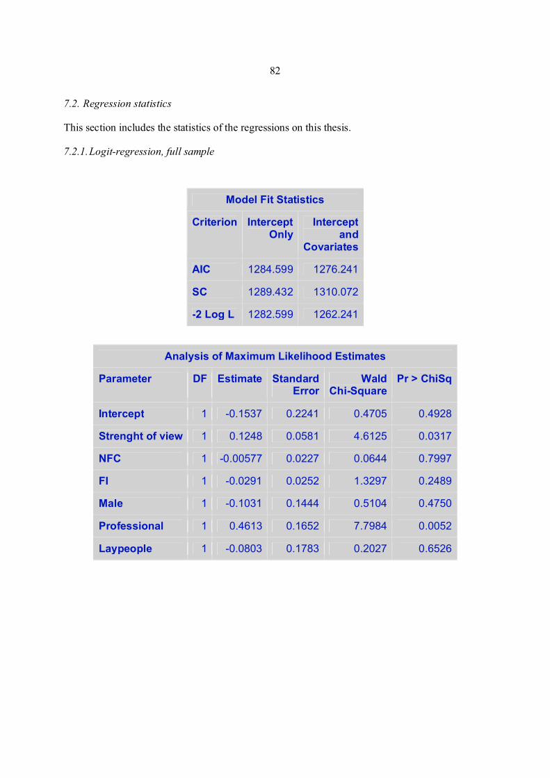
82
7.2. Regression statistics
This section includes the statistics of the regressions on this thesis.
7.2.1. Logit-regression, full sample
Model Fit Statistics
Criterion Intercept Only
Intercept and
Covariates
AIC 1284.599 1276.241
SC 1289.432 1310.072
-2 Log L 1282.599 1262.241
Analysis of Maximum Likelihood Estimates
Parameter DF Estimate Standard Error
W ald Chi-Square
Pr > ChiSq
Intercept 1 -0.1537 0.2241 0.4705 0.4928
Strenght of view 1 0.1248 0.0581 4.6125 0.0317
NFC 1 -0.00577 0.0227 0.0644 0.7997
FI 1 -0.0291 0.0252 1.3297 0.2489
Male 1 -0.1031 0.1444 0.5104 0.4750
Professional 1 0.4613 0.1652 7.7984 0.0052
Laypeople 1 -0.0803 0.1783 0.2027 0.6526
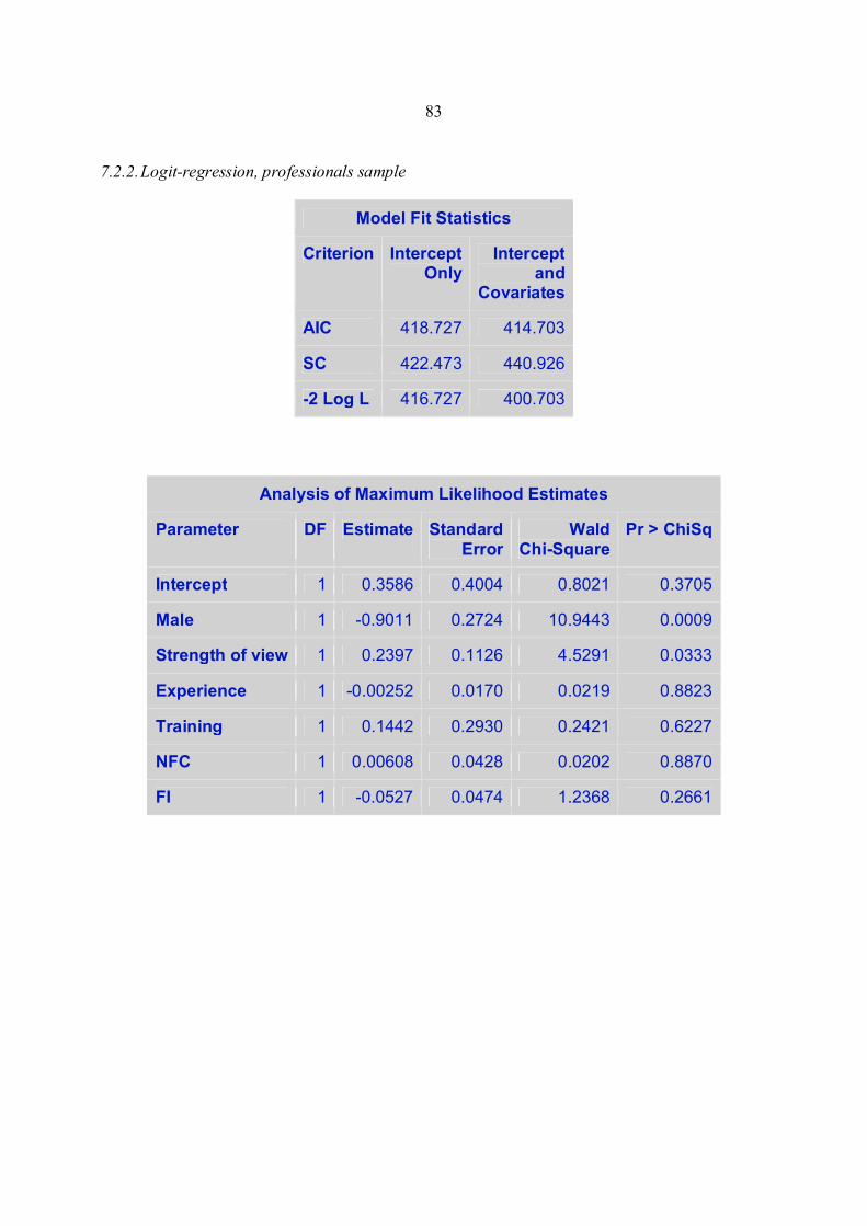
83
7.2.2. Logit-regression, professionals sample
Model Fit Statistics
Criterion Intercept Only
Intercept and
Covariates
AIC 418.727 414.703
SC 422.473 440.926
-2 Log L 416.727 400.703
Analysis of Maximum Likelihood Estimates
Parameter DF Estimate Standard Error
W ald Chi-Square
Pr > ChiSq
Intercept 1 0.3586 0.4004 0.8021 0.3705
Male 1 -0.9011 0.2724 10.9443 0.0009
Strength of view 1 0.2397 0.1126 4.5291 0.0333
Experience 1 -0.00252 0.0170 0.0219 0.8823
Training 1 0.1442 0.2930 0.2421 0.6227
NFC 1 0.00608 0.0428 0.0202 0.8870
FI 1 -0.0527 0.0474 1.2368 0.2661
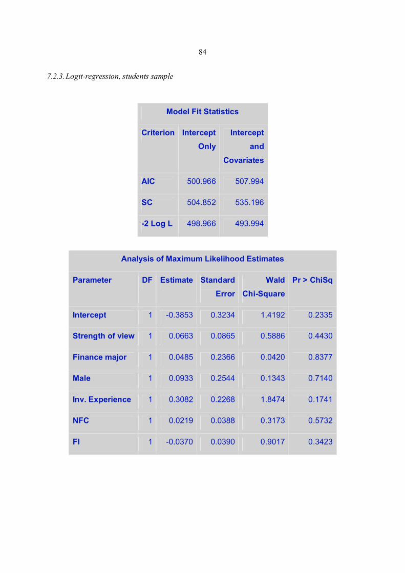
84
7.2.3. Logit-regression, students sample
Model Fit Statistics
Criterion Intercept
Only
Intercept
and
Covariates
AIC 500.966 507.994
SC 504.852 535.196
-2 Log L 498.966 493.994
Analysis of Maximum Likelihood Estimates
Parameter DF Estimate Standard
Error
W ald
Chi-Square
Pr > ChiSq
Intercept 1 -0.3853 0.3234 1.4192 0.2335
Strength of view 1 0.0663 0.0865 0.5886 0.4430
Finance m ajor 1 0.0485 0.2366 0.0420 0.8377
Male 1 0.0933 0.2544 0.1343 0.7140
Inv. Experience 1 0.3082 0.2268 1.8474 0.1741
NFC 1 0.0219 0.0388 0.3173 0.5732
FI 1 -0.0370 0.0390 0.9017 0.3423
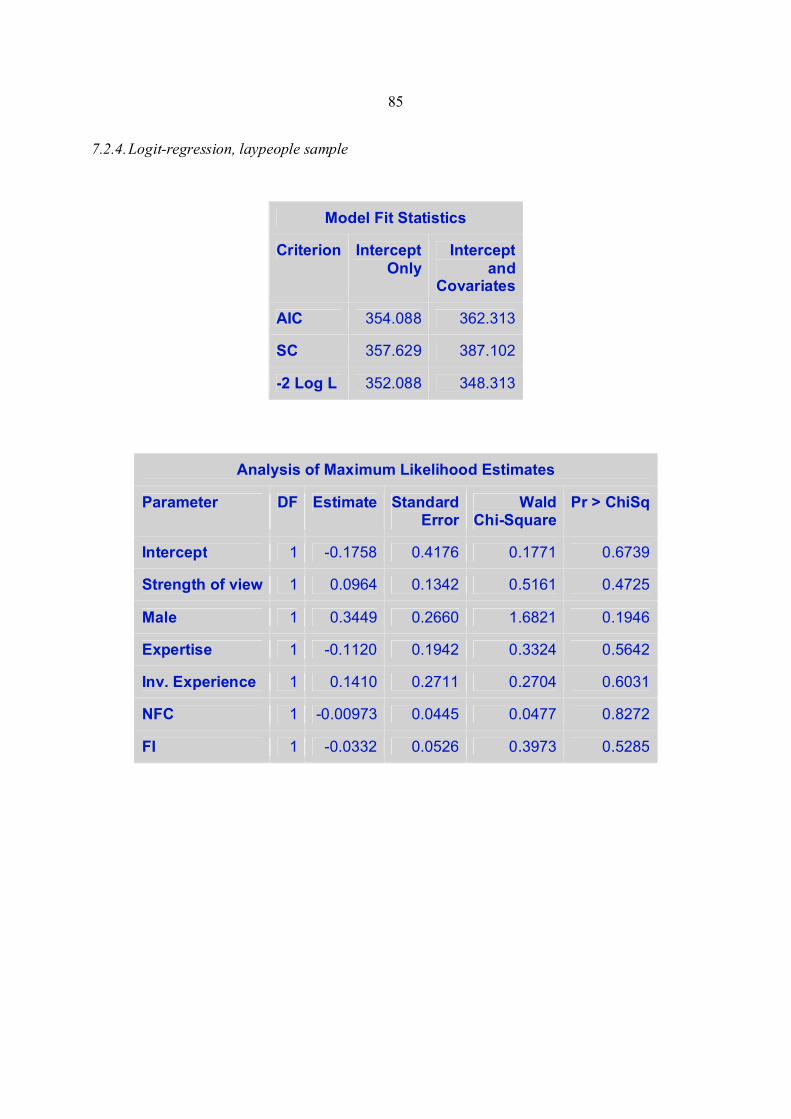
85
7.2.4. Logit-regression, laypeople sample
Model Fit Statistics
Criterion Intercept Only
Intercept and
Covariates
AIC 354.088 362.313
SC 357.629 387.102
-2 Log L 352.088 348.313
Analysis of Maximum Likelihood Estimates
Parameter DF Estimate Standard Error
W ald Chi-Square
Pr > ChiSq
Intercept 1 -0.1758 0.4176 0.1771 0.6739
Strength of view 1 0.0964 0.1342 0.5161 0.4725
Male 1 0.3449 0.2660 1.6821 0.1946
Expertise 1 -0.1120 0.1942 0.3324 0.5642
Inv. Experience 1 0.1410 0.2711 0.2704 0.6031
NFC 1 -0.00973 0.0445 0.0477 0.8272
FI 1 -0.0332 0.0526 0.3973 0.5285

86
7.2.5. OLS-regression
Regression Statistics
Multiple R 0,31277622
R Square 0,09782896
Adjusted R Square 0,08997033
Standard Error 1,17047615
Observations 580
ANOVA
df SS MS F Significance F
Regression 5 85,274 17,055 12,449 0,000
Residual 574 786,388 1,370
Total 579 871,662
Coefficients Standard Error t Stat P-value Lower 95% Upper 95%
Intercept 2,584 0,125 20,722 0,000 2,339 2,829
Professional (d) -0,404 0,122 -3,314 0,001 -0,643 -0,165
Laypeople (d) -0,794 0,124 -6,385 0,000 -1,038 -0,550
Male (d) 0,239 0,104 2,286 0,023 0,034 0,444
NFC 0,002 0,016 0,115 0,908 -0,030 0,034
FI 0,063 0,018 3,537 0,000 0,028 0,099
7.3. Questionnaire sheets
This section includes the questionnaire sheets used in the field surveys. The order of the
questionnaires is:
1. professional group 1, phase 1
2. professional group 1, phase 2
3. professional group 2, phase 1
4. professional group 2, phase 2
5. professional group 3, phase 1
6. professional group 3, phase 2
7. student group, phase 1
8. student group phase 2
9. laypeople group, phase 1
10. laypeople group, phase 2
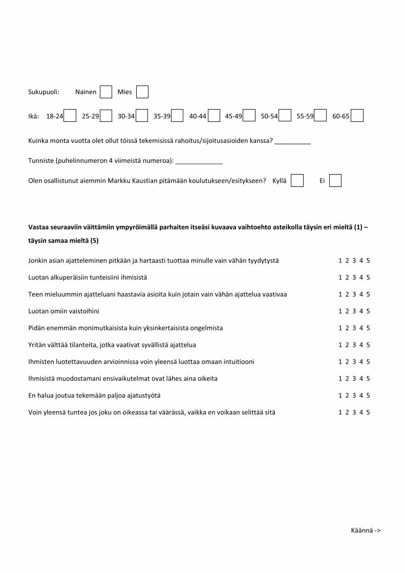
�
�
���������� ��� �� �� �� �
����� ������ ������ ������ ������ ������ ������ ������ ������ ������
���������������������� ��������� ������ � ��������!�"�����#��$����������% ��������&�''''''''''�
(������ �)��" ������ !��������� �������� !��*�'''''''''''''�
+� ����������������� �������!������������������������������� �# ���,�� �&� �,���� -��
�
�
������������������� ��� ���� ������������������������������������������������������ �����������
�������� ��� ���������
.�������������$��� � ��� ����������$��"�!��������������������� ��������"����,,%,�,���� � � ��������������
/����������� !����������� ��������"��������� � � � � � � � ��������������
( ���� ���������$��� ������"����������������������$�������������"����$��� ������������� � � ��������������
/�������������������"����� � � � � � � � � � ��������������
0�%��� � ��������������������������,����� !�����������1 ������� � � � � ��������������
2!������������������� ���3�$���������������,����������$��� ���� � � � � � ��������������
�"���� ������ ������% ���!����������������,� ������������������������������ � � � ��������������
�"�����������%��������� ��������� ������������" ���������� ����� � � � � ��������������
-��"�����$������� � ��������$����$�����, ��� � � � � � � � ��������������
4����,� �������� ��$���$���������� ������������!����3�������� ����������� ������������ � � ��������������
�
�
�
�
�
�
��������5�

��
��
7�
��
��
���
���
���
���
���
���������������������������������
4 ������ ������� � 8!���������� ������� �
� �!�������� �������� ��� ����� ���� �� ��"% ��!��� � "��,�� ���� �� ���� ��� ������% ���9� ( "������� ��� ������� ��!�����
� !��%����� ��9�� :� �79��� ��! ����� � � ��,��� ��"% 3� ������ ���� ��� �,�� ��� ����������3� �������� ��! �����
� "���,���� ��"� �� ������� � !��%����� � ��� �� ����� � ����� �� !�$���!���3������� �������� ��"� �� ������� � !��%����� ��� ��;�
��% ���� ��,,% ���9� � � � �
� � � � � � � � � �
�
�
�
�
�
� � � � � � � � � �
�
�
� � � � � � � � � �
�
�
�
� � � � � � � � � �
�
�
�
�
� � � � � � � � � �
� � � � � � � � � �
�
�
�
�
�
�
������������� ��������
��
��
���
���
���
���
���
��!"#��������!"$�%
-<=��-� -<=�>80
��
���
���
���
���
���
&�'����������
8! ���?�$, �����
/����� !��%�������! ������ � ��,,3�,��,! ��
4 ��$�� � 8!�������
4�!����� ����� �������� ���3�,��,! ��
0�"%����!���������������������������4�"������ �,��
-����� �������$�����������3�;� ''''''''''�
2��!�$��������$���������� 3�;� ''''''''''�
@��!�$��������$���������� 3�;� ''''''''''�
/����� !��%�������! ������ � ��,,3�,��,! ��
-<=��-�� -<=�>80�
4�!����� ����� �������� ���3�,��,! ��
0�"%����!���������������������������4�"������ �,��
-����� �������$�����������3�;� ''''''''''�
2��!�$��������$���������� 3�;� ''''''''''�
@��!�$��������$���������� 3�;� ''''''''''�
/����� !��%�������! ������ � ��,,3�,��,! ��
?�$,� � ������
4�!����� ����� �������� ���3�,��,! ��
0�"%����!���������������������������4�"������ �,��
-����� �������$�����������3�;� ''''''''''�
2��!�$��������$���������� 3�;� ''''''''''�
@��!�$��������$���������� 3�;� ''''''''''�

Tunniste (puhelinnumeron 4 viimeistä numeroa): _____________
Tutkimuksen ensimmäisessä vaiheessa pyysimme teitä valitsemaan periodilla 26.9.2008 – 17.10.2008 paremmin
menestyvät kohteet kolmesta parista, ennustamaan paremmin kehittyvien kohteiden tuotot periodilla sekä
asettamaan tuotoille 90% varmuutta vastaavat raja-arvot. Alla näet kohteiden toteutuneet tuotot (paremmin
menestynyt kohde ympyröity).
Venäläiset osakkeet, tuotto: Brasilialaiset osakkeet, tuotto:
SEK, tuotto: GBP, tuotto:
Öljy, tuotto: Kulta, tuotto:
Palauta nyt mieleesi edellisellä kerralla tekemäsi valinnat sekä antamasi arviot. Tehtäväsi on täyttää edellisellä kerralla
antamasi vastaukset alla oleviin laatikoihin.
Valintani paremmin menestyväksi kohteesta, ympyröi Venäjä Brasilia
Varmuus ennusteen osumisesta, ympyröi Puhdas arvaus 1 2 3 4 5 Vahva näkemys
Ennuste voittajan tuotosta, % __________
Yläraja voittajan tuotolle, % __________ Alaraja voittajan tuotolle, % __________
Valintani paremmin menestyväksi kohteesta, ympyröi SEK GBP
Varmuus ennusteen osumisesta, ympyröi Puhdas arvaus 1 2 3 4 5 Vahva näkemys
Ennuste voittajan tuotosta, % __________
Yläraja voittajan tuotolle, % __________ Alaraja voittajan tuotolle, % __________
Valintani paremmin menestyväksi kohteesta, ympyröi Öljy Kulta
Varmuus ennusteen osumisesta, ympyröi Puhdas arvaus 1 2 3 4 5 Vahva näkemys
Ennuste voittajan tuotosta, % __________
Yläraja voittajan tuotolle, % __________ Alaraja voittajan tuotolle, % __________
Käännä ->
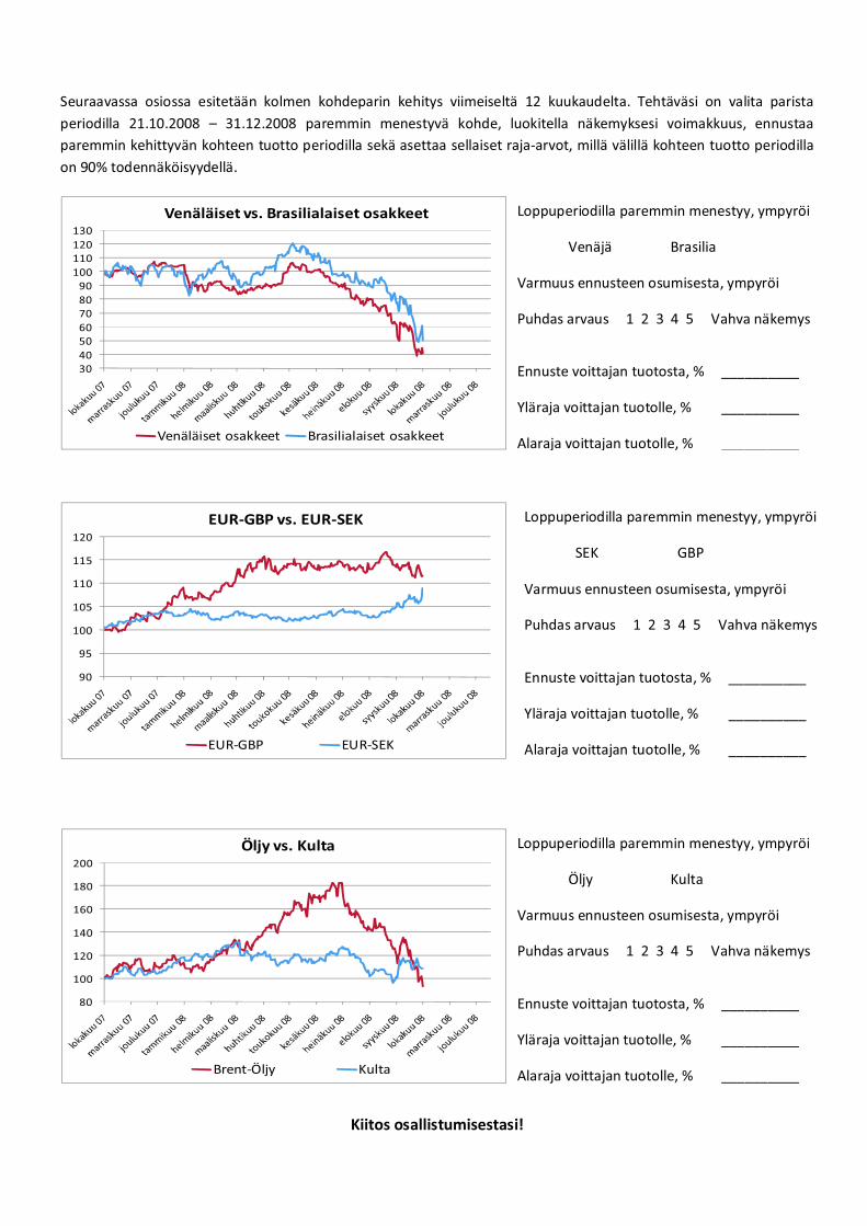
Seuraavassa osiossa esitetään kolmen kohdeparin kehitys viimeiseltä 12 kuukaudelta. Tehtäväsi on valita parista
periodilla 21.10.2008 – 31.12.2008 paremmin menestyvä kohde, luokitella näkemyksesi voimakkuus, ennustaa
paremmin kehittyvän kohteen tuotto periodilla sekä asettaa sellaiset raja-arvot, millä välillä kohteen tuotto periodilla
on 90% todennäköisyydellä.
Kiitos osallistum isestasi!
Loppuperiodilla paremmin menestyy, ympyröi
Venäjä Brasilia
Varmuus ennusteen osumisesta, ympyröi
Puhdas arvaus 1 2 3 4 5 Vahva näkemys
Ennuste voittajan tuotosta, % __________
Yläraja voittajan tuotolle, % __________
Alaraja voittajan tuotolle, % __________
Loppuperiodilla paremmin menestyy, ympyröi
SEK GBP
Varmuus ennusteen osumisesta, ympyröi
Puhdas arvaus 1 2 3 4 5 Vahva näkemys
Ennuste voittajan tuotosta, % __________
Yläraja voittajan tuotolle, % __________
Alaraja voittajan tuotolle, % __________
Loppuperiodilla paremmin menestyy, ympyröi
Öljy Kulta
Varmuus ennusteen osumisesta, ympyröi
Puhdas arvaus 1 2 3 4 5 Vahva näkemys
Ennuste voittajan tuotosta, % __________
Yläraja voittajan tuotolle, % __________
Alaraja voittajan tuotolle, % __________
30
40
50
60
70
80
90
100
110
120
130
Venäläiset vs. Brasilialaiset osakkeet
Venäläiset osakkeet Brasilialaiset osakkeet
90
95
100
105
110
115
120
EU R-GBP vs. EU R-SEK
EU R-GBP EU R-SEK
80
100
120
140
160
180
200
Ö ljy vs. Kulta
Brent-Öljy Kulta

�
�
���������� ��� �� �� �� �
����� ������ ������ ������ ������ ������ ������ ������ ������ ������
���������������������� ��������� ������ � ��������!�"�����#��$����������% ��������&�''''''''''�
(������ �)��" ������ !��������� �������� !��*�'''''''''''''�
+� ����������������� �������!������������������������������� �# ���,�� �&� �,���� -��
�
�
������������������� ��� ���� ������������������������������������������������������ �����������
�������� ��� ���������
.�������������$��� � ��� ����������$��"�!��������������������� ��������"����,,%,�,���� � � ��������������
/����������� !����������� ��������"��������� � � � � � � � ��������������
( ���� ���������$��� ������"����������������������$�������������"����$��� ������������� � � ��������������
/�������������������"����� � � � � � � � � � ��������������
0�%��� � ��������������������������,����� !�����������1 ������� � � � � ��������������
2!������������������� ���3�$���������������,����������$��� ���� � � � � � ��������������
�"���� ������ ������% ���!����������������,� ������������������������������ � � � ��������������
�"�����������%��������� ��������� ������������" ���������� ����� � � � � ��������������
-��"�����$������� � ��������$����$�����, ��� � � � � � � � ��������������
4����,� �������� ��$���$���������� ������������!����3�������� ����������� ������������ � � ��������������
�
�
�
�
�
�
��������5�
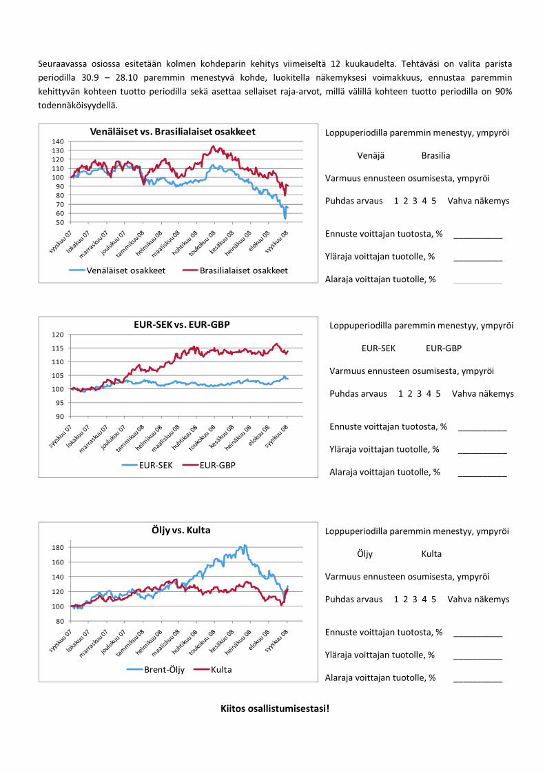
��
��
7�
��
��
���
���
���
���
���
���������������������������������
4 ������ ������� � 8!���������� ������� �
� �!�������� �������� ��� ����� ���� �� ��"% ��!��� � "��,�� ���� �� ���� ��� ������% ���9� ( "������� ��� ������� ��!�����
� !��%����� ��9�� :� ��9��� ��! ����� � � ��,��� ��"% 3� ������ ���� ��� �,�� ��� ����������3� �������� ��! �����
� "���,���� ��"� �� ������� � !��%����� � ��� �� ����� � ����� �� !�$���!���3������� �������� ��"� �� ������� � !��%����� ��� ��;�
��% ���� ��,,% ���9� � � � �
� � � � � � � � � �
�
�
�
�
�
� � � � � � � � � �
�
�
� � � � � � � � � �
�
�
�
� � � � � � � � � �
�
�
�
�
� � � � � � � � � �
� � � � � � � � � �
�
�
�
�
�
�
������������� ��������
��
��
���
���
���
���
���
��!"#��������!"$�%
-<=��-� -<=�>80
��
���
���
���
���
���
&�'����������
8! ���?�$, �����
/����� !��%�������! ������ � ��,,3�,��,! ��
4 ��$�� � 8!�������
4�!����� ����� �������� ���3�,��,! ��
0�"%����!���������������������������4�"������ �,��
-����� �������$�����������3�;� ''''''''''�
2��!�$��������$���������� 3�;� ''''''''''�
@��!�$��������$���������� 3�;� ''''''''''�
/����� !��%�������! ������ � ��,,3�,��,! ��
-<=��-�� -<=�>80�
4�!����� ����� �������� ���3�,��,! ��
0�"%����!���������������������������4�"������ �,��
-����� �������$�����������3�;� ''''''''''�
2��!�$��������$���������� 3�;� ''''''''''�
@��!�$��������$���������� 3�;� ''''''''''�
/����� !��%�������! ������ � ��,,3�,��,! ��
?�$,� � ������
4�!����� ����� �������� ���3�,��,! ��
0�"%����!���������������������������4�"������ �,��
-����� �������$�����������3�;� ''''''''''�
2��!�$��������$���������� 3�;� ''''''''''�
@��!�$��������$���������� 3�;� ''''''''''�

�
�
�
���������� ����������� � ���� � �������� ����� � ����� � �������� � ���������� �� ����������� � �����
�������� ������ ������ � � ���� �� ��� � � � ����� ��������� ������� ������� �������� � ����
��� � � ��������� ���� � ������ � � �� � �� � � ������ !�� � ��� ������� �������� ������� "� �����
�����������������#���$��
�
%��������� �����������&� '(�� � � � )� ���� � ������ �����������&� �'��
*+,��������&� ��'�� � � � � � -).��������&� ��(��
/�����������&� �0�� � � � � � ,��� ��������&� �1��
�
. � �� ���������������������� �� ��������� �� ������ � � ��� �������������������������������������� �� �
� � ���� �� ����� �� �������� ���������2�������������� �� ��� ��� ���� �� ��������� ���� ���� �� �� ���� ����
� ����� �� � �����3��������� �� ��� ��� �� �������4����������#��������� ����������� ��� �� �������
�
�
�
�
�
�
�
�
�
�
�
�
�
�
5���� ���������������� ���������'��(� 5���� ��������� �� ����
% ��� ��� ��������������������� �������#��� � %���� � )� ���� �
% ������������������ �������#�� � � .��� �� �� ����������������'��(�����% �� �������
+��������� � �������� ����6666666666�
7��� � ������ � ������������6666666666� � � !� � � ������ � ������������6666666666�
% ��� ��� ��������������������� �������#��� � *+,� � -).�
% ������������������ �������#�� � � .��� �� �� ����������������'��(�����% �� �������
+��������� � �������� ����6666666666�
7��� � ������ � ������������6666666666� � � !� � � ������ � ������������6666666666�
% ��� ��� ��������������������� �������#��� � /���� � ,��� �
% ������������������ �������#�� � � .��� �� �� ����������������'��(�����% �� �������
+��������� � �������� ����6666666666�
7��� � ������ � ������������6666666666� � � !� � � ������ � ������������6666666666�
,���� 8�
������"����������'�������������� $&�6666666666666�
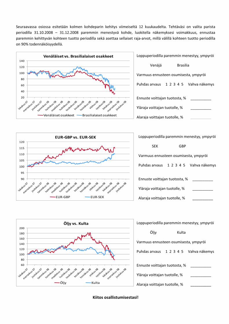
*�� � �� � ������ � ������� ����� ����� ��� ������� ���������� ��� ���� ���� �� ��������� �� � ��� � � ���� �
�������� � ����������� �� ����������� � ����� ������� ������ �������� � ��������� ���� ������� ��� �
� ���������������������������������� ����� ��� ���� ����� � ���������������������������������������� �
�����������#���������� � � � �
� � � � � � � � � �
�
�
�
�
�
� � � � � � � � � �
�
�
� � � � � � � � � �
�
�
�
� � � � � � � � � �
�
�
�
�
� � � � � � � � � �
� � � � � � � � � �
�
�
�
�
�
�
�������������������������
4������������ �� �����������������#��
%���� � )� ���� �
% ������������������ �������#��
.��� �� �� ����������������'��(�����% �� �������
+��������� � �������� ���� 6666666666�
7��� � ������ � ������������ 6666666666�
!� � � ������ � ������������ 6666666666�
4������������ �� �����������������#��
*+,� � -).�
% ������������������ �������#��
.��� �� �� ����������������'��(�����% �� �������
+��������� � �������� ���� 6666666666�
7��� � ������ � ������������ 6666666666�
!� � � ������ � ������������ 6666666666�
4������������ �� �����������������#��
/���� � ,��� �
% ������������������ �������#��
.��� �� �� ����������������'��(�����% �� �������
+��������� � �������� ���� 6666666666�
7��� � ������ � ������������ 6666666666�
!� � � ������ � ������������ 6666666666�
��
'�
1�
��
���
���
�'�
�������������������������������������
%��������� ��� )� ���� � ������ ���
��
�(
���
��(
���
��(
���
�������������������
+ :"-). + :"*+,
1�
��
���
���
�'�
�1�
���
���
�������������
/��� ,���
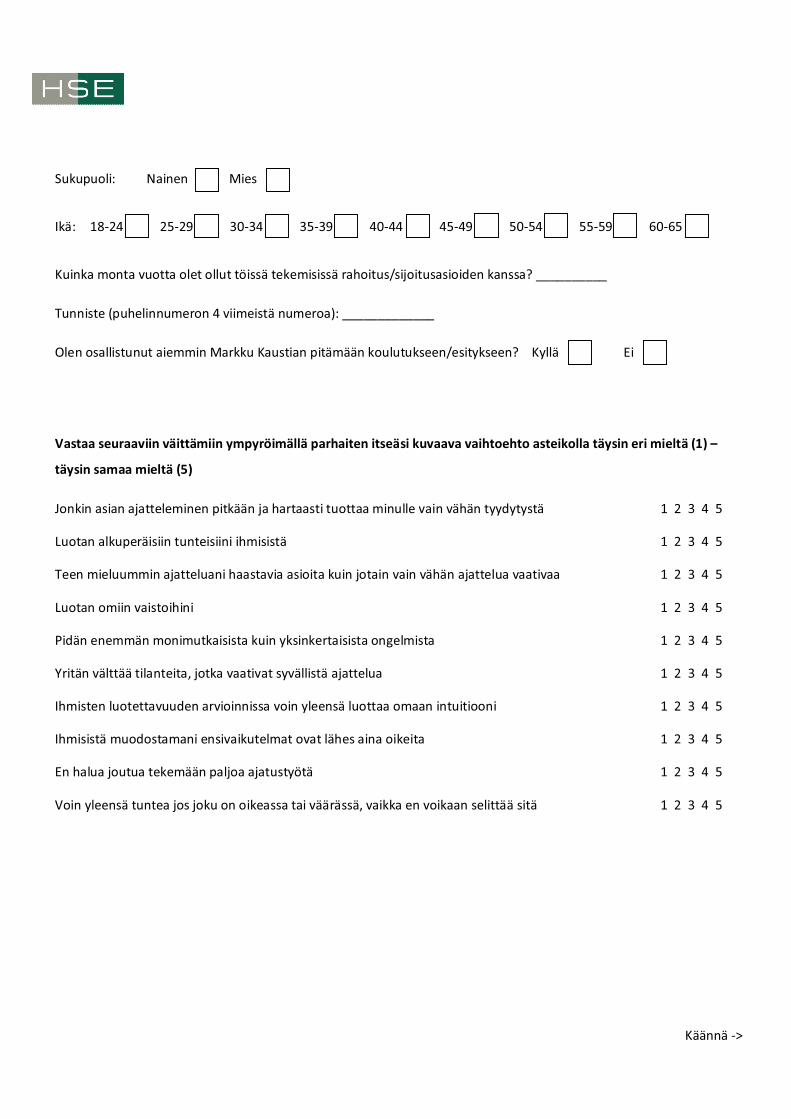
Sukupuoli: Nainen Mies
Ikä: 18-24 25-29 30-34 35-39 40-44 45-49 50-54 55-59 60-65
Kuinka monta vuotta olet ollut töissä tekemisissä rahoitus/sijoitusasioiden kanssa? __________
Tunniste (puhelinnumeron 4 viimeistä numeroa): _____________
Olen osallistunut aiemmin Markku Kaustian pitämään koulutukseen/esitykseen? Kyllä Ei
Vastaa seuraaviin väittämiin ympyröimällä parhaiten itseäsi kuvaava vaihtoehto asteikolla täysin eri mieltä (1) –
täysin samaa mieltä (5)
Jonkin asian ajatteleminen pitkään ja hartaasti tuottaa minulle vain vähän tyydytystä 1 2 3 4 5
Luotan alkuperäisiin tunteisiini ihmisistä 1 2 3 4 5
Teen mieluummin ajatteluani haastavia asioita kuin jotain vain vähän ajattelua vaativaa 1 2 3 4 5
Luotan omiin vaistoihini 1 2 3 4 5
Pidän enemmän monimutkaisista kuin yksinkertaisista ongelmista 1 2 3 4 5
Yritän välttää tilanteita, jotka vaativat syvällistä ajattelua 1 2 3 4 5
Ihmisten luotettavuuden arvioinnissa voin yleensä luottaa omaan intuitiooni 1 2 3 4 5
Ihmisistä muodostamani ensivaikutelmat ovat lähes aina oikeita 1 2 3 4 5
En halua joutua tekemään paljoa ajatustyötä 1 2 3 4 5
Voin yleensä tuntea jos joku on oikeassa tai väärässä, vaikka en voikaan selittää sitä 1 2 3 4 5
Käännä ->
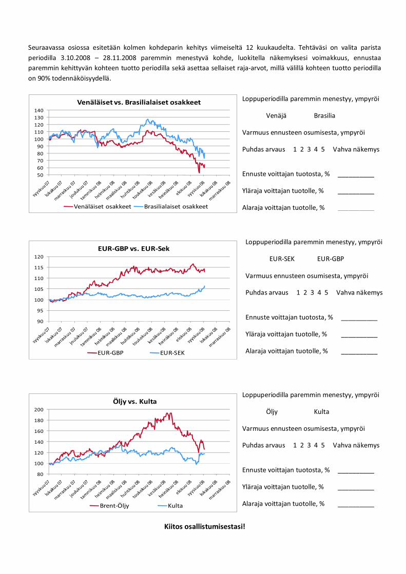
Seuraavassa osiossa esitetään kolmen kohdeparin kehitys viimeiseltä 12 kuukaudelta. Tehtäväsi on valita parista
periodilla 3.10.2008 – 28.11.2008 paremmin menestyvä kohde, luokitella näkemyksesi voimakkuus, ennustaa
paremmin kehittyvän kohteen tuotto periodilla sekä asettaa sellaiset raja-arvot, millä välillä kohteen tuotto periodilla
on 90% todennäköisyydellä.
Kiitos osallistumisestasi!
Loppuperiodilla paremmin menestyy, ympyröi
Venäjä Brasilia
Varmuus ennusteen osumisesta, ympyröi
Puhdas arvaus 1 2 3 4 5 Vahva näkemys
Ennuste voittajan tuotosta, % __________
Yläraja voittajan tuotolle, % __________
Alaraja voittajan tuotolle, % __________
Loppuperiodilla paremmin menestyy, ympyröi
EU R-SEK EU R-G BP
Varmuus ennusteen osumisesta, ympyröi
Puhdas arvaus 1 2 3 4 5 Vahva näkemys
Ennuste voittajan tuotosta, % __________
Yläraja voittajan tuotolle, % __________
Alaraja voittajan tuotolle, % __________
Loppuperiodilla paremmin menestyy, ympyröi
Ö ljy Kulta
Varmuus ennusteen osumisesta, ympyröi
Puhdas arvaus 1 2 3 4 5 Vahva näkemys
Ennuste voittajan tuotosta, % __________
Yläraja voittajan tuotolle, % __________
Alaraja voittajan tuotolle, % __________
50
60
70
80
90
100
110
120
130
140
Venäläiset vs. Brasilialaiset osakkeet
Venäläiset osakkeet Brasilialaiset osakkeet
90
95
100
105
110
115
120
EU R-GBP vs. EU R-Sek
EU R-G BP EU R-SEK
80
100
120
140
160
180
200
Ö ljy vs. Kulta
Brent-Ö ljy Kulta

Tutkimuksen ensimmäisessä vaiheessa pyysimme teitä valitsemaan periodilla 3.10.2008 – 28.11.2008 paremmin
menestyvät kohteet kolmesta parista, ennustamaan paremmin kehittyvien kohteiden tuotot periodilla sekä
asettamaan tuotoille 90% varmuutta vastaavat raja-arvot. Alla näet kohteiden toteutuneet tuotot (paremmin
menestynyt kohde ympyröity).
Venäläiset osakkeet, tuotto: -30% Brasilialaiset osakkeet, tuotto: -22%
SEK, tuotto: -5,4% G BP, tuotto: -5,9%
Ö ljy, tuotto: -41% Kulta, tuotto: -2%
Palauta nyt mieleesi edellisellä kerralla tekemäsi valinnat sekä antamasi arviot. Tehtäväsi on täyttää edellisellä kerralla
antamasi vastaukset alla oleviin laatikoihin. On tärkeää, että vastaat vaikka et tarkasti muistaisikaan omia vastauksiasi.
Tarvittaessa arvioi/päättele omat aiemmat vastauksesi. Luokittele myös se, kuinka hyvin muistat vastauksesi.
Muistan hyvin huonosti 1 2 3 4 5 Muistan erittäin tarkasti
Valintani paremmin menestyväksi kohteesta, ympyröi Venäjä Brasilia
Varmuus ennusteen osumisesta, ympyröi Puhdas arvaus 1 2 3 4 5 Vahva näkemys
Ennuste voittajan tuotosta, % __________
Yläraja voittajan tuotolle, % __________ A laraja voittajan tuotolle, % __________
Valintani paremmin menestyväksi kohteesta, ympyröi SEK G BP
Varmuus ennusteen osumisesta, ympyröi Puhdas arvaus 1 2 3 4 5 Vahva näkemys
Ennuste voittajan tuotosta, % __________
Yläraja voittajan tuotolle, % __________ A laraja voittajan tuotolle, % __________
Valintani paremmin menestyväksi kohteesta, ympyröi Ö ljy Kulta
Varmuus ennusteen osumisesta, ympyröi Puhdas arvaus 1 2 3 4 5 Vahva näkemys
Ennuste voittajan tuotosta, % __________
Yläraja voittajan tuotolle, % __________ A laraja voittajan tuotolle, % __________
Käännä ->
Tunniste (puhelinnumeron 4 viimeistä numeroa): _____________
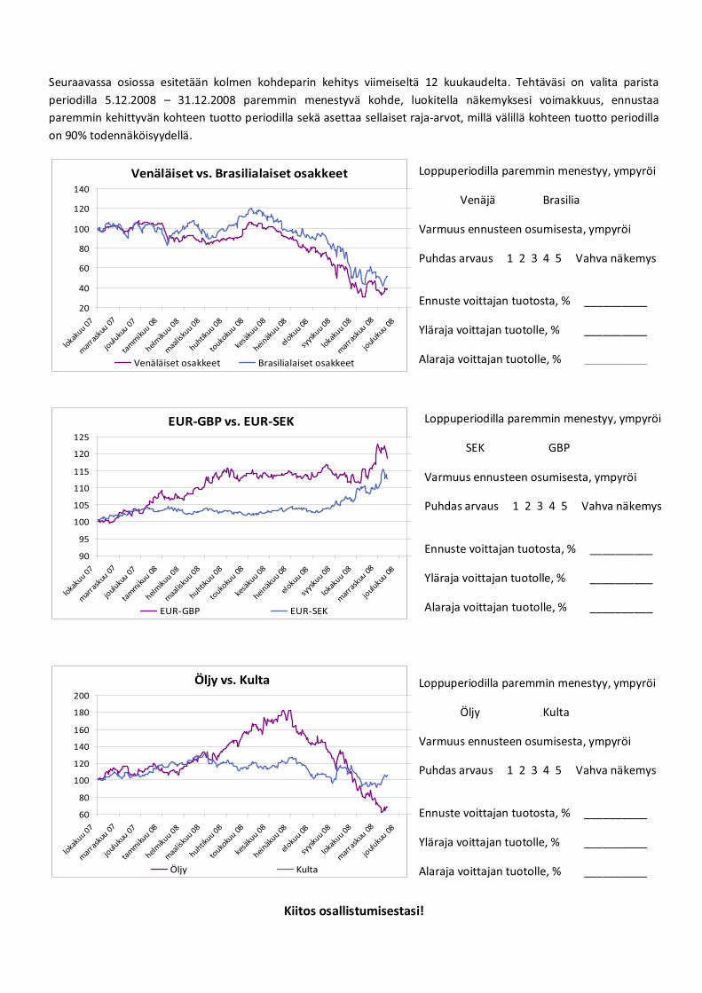
Seuraavassa osiossa esitetään kolmen kohdeparin kehitys viimeiseltä 12 kuukaudelta. Tehtäväsi on valita parista
periodilla 5.12.2008 – 31.12.2008 paremmin menestyvä kohde, luokitella näkemyksesi voimakkuus, ennustaa
paremmin kehittyvän kohteen tuotto periodilla sekä asettaa sellaiset raja-arvot, millä välillä kohteen tuotto periodilla
on 90% todennäköisyydellä.
Kiitos osallistumisestasi!
Loppuperiodilla paremmin menestyy, ympyröi
Venäjä Brasilia
Varmuus ennusteen osumisesta, ympyröi
Puhdas arvaus 1 2 3 4 5 Vahva näkemys
Ennuste voittajan tuotosta, % __________
Yläraja voittajan tuotolle, % __________
Alaraja voittajan tuotolle, % __________
Loppuperiodilla paremmin menestyy, ympyröi
SEK G BP
Varmuus ennusteen osumisesta, ympyröi
Puhdas arvaus 1 2 3 4 5 Vahva näkemys
Ennuste voittajan tuotosta, % __________
Yläraja voittajan tuotolle, % __________
Alaraja voittajan tuotolle, % __________
Loppuperiodilla paremmin menestyy, ympyröi
Ö ljy Kulta
Varmuus ennusteen osumisesta, ympyröi
Puhdas arvaus 1 2 3 4 5 Vahva näkemys
Ennuste voittajan tuotosta, % __________
Yläraja voittajan tuotolle, % __________
Alaraja voittajan tuotolle, % __________
Venäläiset vs. Brasilialaiset osakkeet
20
40
60
80
100
120
140
loka
kuu 0
7
mar
rask
uu 0
7
joul
ukuu
07
tam
mik
uu 08
helm
ikuu 0
8
maa
lisku
u 08
huhtikuu 0
8
touko
kuu 0
8
kesä
kuu 0
8
heinäk
uu 08
eloku
u 08
syys
kuu 0
8
loka
kuu 0
8
mar
rask
uu 0
8
joul
ukuu
08
Venäläiset osakkeet Brasilialaiset osakkeet
EU R-GBP vs. EU R-SEK
90
95
100
105
110
115
120
125
loka
kuu 0
7
mar
rask
uu 0
7
joul
ukuu
07
tam
mik
uu 08
helm
ikuu 0
8
maa
lisku
u 08
huhtikuu 0
8
touko
kuu 0
8
kesä
kuu 0
8
heinäk
uu 08
eloku
u 08
syys
kuu 0
8
loka
kuu 0
8
mar
rask
uu 0
8
joul
ukuu
08
EU R-GBP EU R-SEK
Ö ljy vs. Kulta
60
80
100
120
140
160
180
200
loka
kuu 0
7
mar
rask
uu 0
7
joul
ukuu
07
tam
mik
uu 08
helm
ikuu 0
8
maa
lisku
u 08
huhtikuu 0
8
touko
kuu 0
8
kesä
kuu 0
8
heinäk
uu 08
eloku
u 08
syys
kuu 0
8
loka
kuu 0
8
mar
rask
uu 0
8
joul
ukuu
08
Ö ljy Kulta

This questionnaire is part of a Master’s Thesis study at H SE. The questionnaire contains tw o sides. The first side asks
for background information. The second side contains investment related questions. Please make sure you answer all
questions on both sides of the paper, otherw ise your answ ers can not be used. If you are unsure about some answ ers,
make a guess anyw ay. The study has tw o phases, the first one today and the second one on 14.11.2008 (also a CoFi
exercise session). It is important to participate in both phases – there w ill be a reward for everyone participating in the
second phase. How ever, please answ er now even if you can’t participate in the second phase.
Sex: Female Male
Age: 18-24 25-29 30-34 35-39 40-44 45-49 50-54 55-59 60-65
Major: _________________________________
H ave you made any stock market investments yourself? Yes No
D o you have any w ork experience in the field of finance? If yes, how many years? ____________
Matching code (= last 4 digits of your phone number): _____________ (needed to match your 2nd phase answ ers)
A nsw er the follow ing statements by circulating the choice that best describes yourself on the scale totally disagree (1) – totally agree (5)
Thinking hard and for a long time about something gives me little satisfaction 1 2 3 4 5
I trust my initial feelings about people 1 2 3 4 5
I prefer to do something that challenges my thinking abilities rather
than something that requires little thought 1 2 3 4 5
I believe in trusting my hunches 1 2 3 4 5
I prefer complex to simple problems 1 2 3 4 5
I try to avoid situations that require thinking in depth about something 1 2 3 4 5
W hen it comes to trusting people, I can usually rely on my "gut feelings" 1 2 3 4 5
My initial impressions of people are almost alw ays right 1 2 3 4 5
I don't like to have to do a lot of thinking 1 2 3 4 5
I can usually feel w hen a person is right or w rong even if I can't explain how I know 1 2 3 4 5
Turn ->
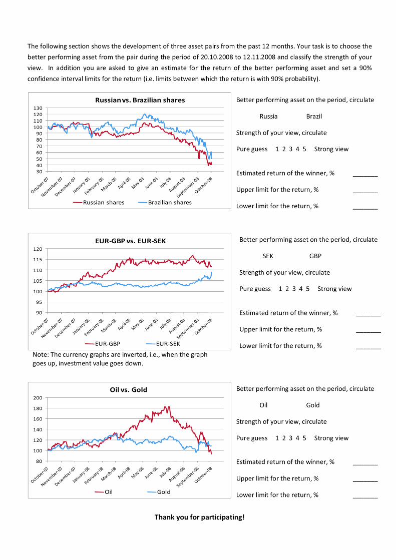
The follow ing section show s the development of three asset pairs from the past 12 months. Your task is to choose the
better performing asset from the pair during the period of 20.10.2008 to 12.11.2008 and classify the strength of your
view . In addition you are asked to give an estimate for the return of the better performing asset and set a 90%
confidence interval limits for the return (i.e. limits betw een w hich the return is w ith 90% probability).
Thank you for participating!
Note: The currency graphs are inverted, i.e., w hen the graph
goes up, investment value goes dow n.
Better performing asset on the period, circulate
Russia Brazil
Strength of your view , circulate
Pure guess 1 2 3 4 5 Strong view
Estimated return of the w inner, % _______
U pper limit for the return, % _______
Low er limit for the return, % _______
Better performing asset on the period, circulate
SEK G BP
Strength of your view , circulate
Pure guess 1 2 3 4 5 Strong view
Estimated return of the w inner, % _______
U pper limit for the return, % _______
Low er limit for the return, % _______
Better performing asset on the period, circulate
Oil G old
Strength of your view , circulate
Pure guess 1 2 3 4 5 Strong view
Estimated return of the w inner, % _______
U pper limit for the return, % _______
Low er limit for the return, % _______
30
40
50
60
70
80
90
100
110
120
130
Russian vs. Brazilian shares
Russian shares Brazilian shares
90
95
100
105
110
115
120
EU R-G BP vs. EU R-SEK
EU R-GBP EU R-SEK
80
100
120
140
160
180
200
O il vs. Gold
Oil Gold

Matching code (= last 4 digits of your phone number): _____________ (needed to match your 1st phase answ ers)
In first phase of the study you w ere asked to choose the better performing assets from the three pairs on 20.10.2008
to 12.11.2008 period. In addition you w ere asked to estimate the return of the better performing asset and set 90%
confidence interval limits for the return. H ere you can see the realized returns (asset w ith higher return is circulated,
i.e. the w inner).
Russian shares, return: +6% Brazilian shares, return: -15%
SEK, return: -1.6% G BP, return: -6.7%
Oil, return: -24% G old, return: -9%
Now try to remember the answ ers and estimates you gave last time. Your task now is to fill the answ ers from the first
phase to the boxes below . It is very important that you answ er now even though you could not remember you initial
answ ers very w ell. If so, please estimate/conclude your initial answ ers. Classify also how w ell you can remember your
initial answ ers.
Turn ->
My selection for the better performing asset, circulate Russia Brazil
Strength of your view , circulate Pure guess 1 2 3 4 5 Strong view
Estimated return of the w inner, % __________
U pper limit for the return, % __________ Low er limit for the return, % __________
My selection for the better performing asset, circulate SEK G BP
Strength of your view , circulate Pure guess 1 2 3 4 5 Strong view
Estimated return of the w inner, % __________
U pper limit for the return, % __________ Low er limit for the return, % __________
My selection for the better performing asset, circulate Oil G old
Strength of your view , circulate Pure guess 1 2 3 4 5 Strong view
Estimated return of the w inner, % __________
U pper limit for the return, % __________ Low er limit for the return, % __________
I remember poorly 1 2 3 4 5 I remember clearly
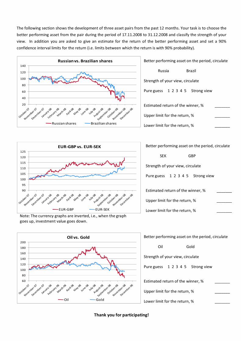
The follow ing section show s the development of three asset pairs from the past 12 months. Your task is to choose the
better performing asset from the pair during the period of 17.11.2008 to 31.12.2008 and classify the strength of your
view . In addition you are asked to give an estimate for the return of the better performing asset and set a 90%
confidence interval limits for the return (i.e. limits betw een w hich the return is w ith 90% probability).
Thank you for participating!
Note: The currency graphs are inverted, i.e., w hen the graph
goes up, investment value goes dow n.
Better performing asset on the period, circulate
Russia Brazil
Strength of your view , circulate
Pure guess 1 2 3 4 5 Strong view
Estimated return of the w inner, % _______
U pper limit for the return, % _______
Low er limit for the return, % _______
Better performing asset on the period, circulate
SEK G BP
Strength of your view , circulate
Pure guess 1 2 3 4 5 Strong view
Estimated return of the w inner, % _______
U pper limit for the return, % _______
Low er limit for the return, % _______
Better performing asset on the period, circulate
Oil G old
Strength of your view , circulate
Pure guess 1 2 3 4 5 Strong view
Estimated return of the w inner, % _______
U pper limit for the return, % _______
Low er limit for the return, % _______
20
40
60
80
100
120
140
Russian vs. Brazilian shares
Russian shares Brazilian shares
90
95
100
105
110
115
120
125
EU R-G BP vs. EU R-SEK
EU R-G BP EU R-SEK
60
80
100
120
140
160
180
200
O il vs. G old
Oil G old
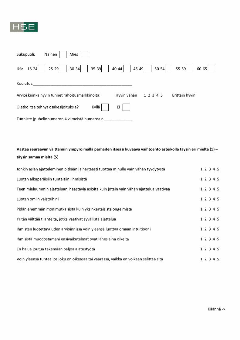
Sukupuoli: Nainen Mies
Ikä: 18-24 25-29 30-34 35-39 40-44 45-49 50-54 55-59 60-65
Koulutus:______________________________________________
Arvioi kuinka hyvin tunnet rahoitusmarkkinoita: H yvin vähän 1 2 3 4 5 Erittäin hyvin
Oletko itse tehnyt osakesijoituksia? Kyllä Ei
Tunniste (puhelinnumeron 4 viimeistä numeroa): _____________
Vastaa seuraaviin väittämiin ympyröimällä parhaiten itseäsi kuvaava vaihtoehto asteikolla täysin eri mieltä (1) –
täysin samaa mieltä (5)
Jonkin asian ajatteleminen pitkään ja hartaasti tuottaa minulle vain vähän tyydytystä 1 2 3 4 5
Luotan alkuperäisiin tunteisiini ihmisistä 1 2 3 4 5
Teen mieluummin ajatteluani haastavia asioita kuin jotain vain vähän ajattelua vaativaa 1 2 3 4 5
Luotan omiin vaistoihini 1 2 3 4 5
Pidän enemmän monimutkaisista kuin yksinkertaisista ongelmista 1 2 3 4 5
Yritän välttää tilanteita, jotka vaativat syvällistä ajattelua 1 2 3 4 5
Ihmisten luotettavuuden arvioinnissa voin yleensä luottaa omaan intuitiooni 1 2 3 4 5
Ihmisistä muodostamani ensivaikutelmat ovat lähes aina oikeita 1 2 3 4 5
En halua joutua tekemään paljoa ajatustyötä 1 2 3 4 5
Voin yleensä tuntea jos joku on oikeassa tai väärässä, vaikka en voikaan selittää sitä 1 2 3 4 5
Käännä ->
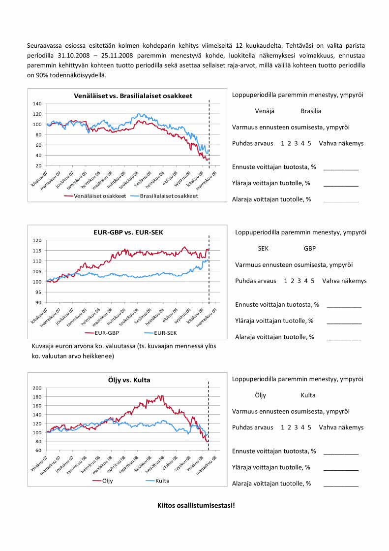
Seuraavassa osiossa esitetään kolmen kohdeparin kehitys viimeiseltä 12 kuukaudelta. Tehtäväsi on valita parista
periodilla 31.10.2008 – 25.11.2008 paremmin menestyvä kohde, luokitella näkemyksesi voimakkuus, ennustaa
paremmin kehittyvän kohteen tuotto periodilla sekä asettaa sellaiset raja-arvot, millä välillä kohteen tuotto periodilla
on 90% todennäköisyydellä.
Kiitos osallistumisestasi!
Loppuperiodilla paremmin menestyy, ympyröi
Venäjä Brasilia
Varmuus ennusteen osumisesta, ympyröi
Puhdas arvaus 1 2 3 4 5 Vahva näkemys
Ennuste voittajan tuotosta, % __________
Yläraja voittajan tuotolle, % __________
Alaraja voittajan tuotolle, % __________
Loppuperiodilla paremmin menestyy, ympyröi
SEK G BP
Varmuus ennusteen osumisesta, ympyröi
Puhdas arvaus 1 2 3 4 5 Vahva näkemys
Ennuste voittajan tuotosta, % __________
Yläraja voittajan tuotolle, % __________
Alaraja voittajan tuotolle, % __________
Loppuperiodilla paremmin menestyy, ympyröi
Ö ljy Kulta
Varmuus ennusteen osumisesta, ympyröi
Puhdas arvaus 1 2 3 4 5 Vahva näkemys
Ennuste voittajan tuotosta, % __________
Yläraja voittajan tuotolle, % __________
Alaraja voittajan tuotolle, % __________
20
40
60
80
100
120
140
Venäläiset vs. Brasilialaiset osakkeet
Venäläiset osakkeet Brasilialaiset osakkeet
90
95
100
105
110
115
120
EU R-GBP vs. EU R-SEK
EU R-G BP EU R-SEK
60
80
100
120
140
160
180
200
Ö ljy vs. Kulta
Ö ljy Kulta
Kuvaaja euron arvona ko. valuutassa (ts. kuvaajan mennessä ylös
ko. valuutan arvo heikkenee)

Tutkimuksen ensimmäisessä vaiheessa pyysimme teitä valitsemaan periodilla 31.10.2008 – 25.11.2008 paremmin
menestyvät kohteet kolmesta parista, ennustamaan paremmin kehittyvien kohteiden tuotot periodilla sekä
asettamaan tuotoille 90% varmuutta vastaavat raja-arvot. Alla näet kohteiden toteutuneet tuotot (paremmin
menestynyt kohde ympyröity).
Venäläiset osakkeet, tuotto: -12% Brasilialaiset osakkeet, tuotto: -17%
SEK, tuotto: -3,7% G BP, tuotto: -7,6%
Ö ljy, tuotto: -25% Kulta, tuotto: +14%
Palauta nyt mieleesi edellisellä kerralla tekemäsi valinnat sekä antamasi arviot. Tehtäväsi on täyttää edellisellä kerralla
antamasi vastaukset alla oleviin laatikoihin. On tärkeää, että vastaat vaikka et tarkasti muistaisikaan omia vastauksiasi.
Tarvittaessa arvioi/päättele omat aiemmat vastauksesi. Luokittele myös se, kuinka hyvin muistat vastauksesi.
Muistan hyvin huonosti 1 2 3 4 5 Muistan erittäin tarkasti
Valintani paremmin menestyväksi kohteesta, ympyröi Venäjä Brasilia
Varmuus ennusteen osumisesta, ympyröi Puhdas arvaus 1 2 3 4 5 Vahva näkemys
Ennuste voittajan tuotosta, % __________
Yläraja voittajan tuotolle, % __________ A laraja voittajan tuotolle, % __________
Valintani paremmin menestyväksi kohteesta, ympyröi SEK G BP
Varmuus ennusteen osumisesta, ympyröi Puhdas arvaus 1 2 3 4 5 Vahva näkemys
Ennuste voittajan tuotosta, % __________
Yläraja voittajan tuotolle, % __________ A laraja voittajan tuotolle, % __________
Valintani paremmin menestyväksi kohteesta, ympyröi Ö ljy Kulta
Varmuus ennusteen osumisesta, ympyröi Puhdas arvaus 1 2 3 4 5 Vahva näkemys
Ennuste voittajan tuotosta, % __________
Yläraja voittajan tuotolle, % __________ A laraja voittajan tuotolle, % __________
Käännä ->
Tunniste (puhelinnumeron 4 viimeistä numeroa): _____________
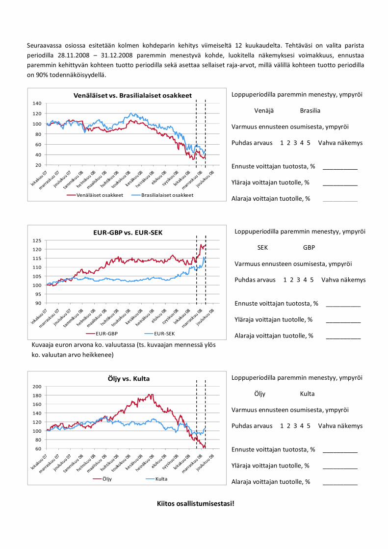
Seuraavassa osiossa esitetään kolmen kohdeparin kehitys viimeiseltä 12 kuukaudelta. Tehtäväsi on valita parista
periodilla 28.11.2008 – 31.12.2008 paremmin menestyvä kohde, luokitella näkemyksesi voimakkuus, ennustaa
paremmin kehittyvän kohteen tuotto periodilla sekä asettaa sellaiset raja-arvot, millä välillä kohteen tuotto periodilla
on 90% todennäköisyydellä.
Kiitos osallistumisestasi!
Loppuperiodilla paremmin menestyy, ympyröi
Venäjä Brasilia
Varmuus ennusteen osumisesta, ympyröi
Puhdas arvaus 1 2 3 4 5 Vahva näkemys
Ennuste voittajan tuotosta, % __________
Yläraja voittajan tuotolle, % __________
Alaraja voittajan tuotolle, % __________
Loppuperiodilla paremmin menestyy, ympyröi
SEK G BP
Varmuus ennusteen osumisesta, ympyröi
Puhdas arvaus 1 2 3 4 5 Vahva näkemys
Ennuste voittajan tuotosta, % __________
Yläraja voittajan tuotolle, % __________
Alaraja voittajan tuotolle, % __________
Loppuperiodilla paremmin menestyy, ympyröi
Ö ljy Kulta
Varmuus ennusteen osumisesta, ympyröi
Puhdas arvaus 1 2 3 4 5 Vahva näkemys
Ennuste voittajan tuotosta, % __________
Yläraja voittajan tuotolle, % __________
Alaraja voittajan tuotolle, % __________
20
40
60
80
100
120
140
Venäläiset vs. Brasilialaiset osakkeet
Venäläiset osakkeet Brasilialaiset osakkeet
60
80
100
120
140
160
180
200
Ö ljy vs. Kulta
Ö ljy Kulta
Kuvaaja euron arvona ko. valuutassa (ts. kuvaajan mennessä ylös
ko. valuutan arvo heikkenee)
90
95
100
105
110
115
120
125
EU R-G BP vs. EU R-SEK
EU R-G BP EU R-SEK