belief propagation tutorialquestions • what is the most probable conﬁguration? • what is the...

Belief Propagation Tutorial

Jonathan YedidiaMitsubishi Electric Research Labs

Outline

• Factor Graphs

• Message Passing Algorithms

• Free Energy Approximations

A B C

1 2 3 4

Variable Nodes

Factor Nodes

A B C

1 2 3 4

A B C

1 2 3 4

Brief Article

The Author

March 20, 2008

p(X) =1Z

exp

!!

"

a

Ea(Xa)

#(1)

1

Questions• What is the most probable configuration?

• What is the marginal probability for a node or group of nodes?

These questions can be attacked by Simulated Annealing or Monte Carlo Simulation, but there are often much more efficient methods.

Belief propagation is one method, but one should remember that there are others!

Marginal Probabilities = local magnetization

Ising Model

Computer Vision and Signal Processing

Marginal Probabilities = “beliefs” about possible underlying scenes

Observed Variables

=

Observed Variables induce a local “evidence” factor node.

Error-correcting Codes

+ + +

Marginal Probabilities = A posteriori bit probabilities

(Tanner, 1981 Gallager, 1963)

Inference Engines

A S

T L B

E

D

X(example adapted from Lauritzen, 1992)

Marginal Probabilities = “beliefs” about possible diagnoses

(Pearl, 1988)

Equivalent Graphical Models

• Markov Random Fields: Use only variable nodes. Factor nodes are defined implicitly when all nodes in a “clique” are connected to each other.

• Forney Factor Graphs: Use only factor nodes. Variables live on edges. Use equality factor nodes to convert ordinary factor graphs into Forney factor graphs

• Bayesian Networks: Use directed graphs which imply conditional probabilities.

Outline

• Factor Graphs



Brief Article

The Author

March 20, 2008

p(X) =1Z

exp

!!

"

a

Ea(Xa)

#(1)

F = U ! TS ="

s

psEs + T"

s

ps log ps (2)

G(bs) ="

s

bsEs + T"

s

bs log bs (3)

bs =1Z

exp (!Es/T ) (4)

bi(xi) "$

a!N(i)

ma"i(xi) (5)

1

Belief Propagation

i

“beliefs” “messages”

a

The “belief” is the BP approximation of the marginal probability.

Brief Article

The Author

March 20, 2008

p(X) =1Z

exp

!!

"

a

Ea(Xa)

#(1)

F = U ! TS ="

s

psEs + T"

s

ps log ps (2)

G(bs) ="

s

bsEs + T"

s

bs log bs (3)

bs =1Z

exp (!Es/T ) (4)

bi(xi) "$

a!N(i)

ma"i(xi) (5)

ba(Xa) " fa(Xa)$

i!N(a)

$

b!N(i)\a

mb"i(xi) (6)

1

BP Message-update Rules

Using we get the “Sum-Product” message-update rules:

aii a=

Brief Article

The Author

March 20, 2008

p(X) =1Z

exp

!!

"

a

Ea(Xa)

#(1)

F = U ! TS ="

s

psEs + T"

s

ps log ps (2)

G(bs) ="

s

bsEs + T"

s

bs log bs (3)

bs =1Z

exp (!Es/T ) (4)

bi(xi) "$

a!N(i)

ma"i(xi) (5)

ba(Xa) " fa(Xa)$

i!N(a)

$

b!N(i)\a

mb"i(xi) (6)

bi(xi) ="

Xa\xi

ba(Xa), (7)

1

Brief Article

The Author

March 20, 2008

p(X) =1Z

exp

!!

"

a

Ea(Xa)

#(1)

F = U ! TS ="

s

psEs + T"

s

ps log ps (2)

G(bs) ="

s

bsEs + T"

s

bs log bs (3)

bs =1Z

exp (!Es/T ) (4)

bi(xi) "$

a!N(i)

ma"i(xi) (5)

ba(Xa) " fa(Xa)$

i!N(a)

$

b!N(i)\a

mb"i(xi) (6)

bi(xi) ="

Xa\xi

ba(Xa), (7)

ma"i(xi) ="

Xa\xi

fa(Xa)$

j!N(a)\i

$

b!N(j)\a

mb"j(xj) (8)

1

BP Is Exact for Trees

A B C

1 2 3 4

Brief Article

The Author

March 20, 2008

p(X) =1Z

exp

!!

"

a

Ea(Xa)

#(1)

F = U ! TS ="

s

psEs + T"

s

ps log ps (2)

G(bs) ="

s

bsEs + T"

s

bs log bs (3)

bs =1Z

exp (!Es/T ) (4)

bi(xi) "$

a!N(i)

ma"i(xi) (5)

ba(Xa) " fa(Xa)$

i!N(a)

$

b!N(i)\a

mb"i(xi) (6)

bi(xi) ="

Xa\xi

ba(Xa), (7)

ma"i(xi) ="

Xa\xi

fa(Xa)$

j!N(a)\i

$

b!N(j)\a

mb"j(xj) (8)

b1(x1) " mA"1(x1) (9)

""

x2

fA(x1, x2)mB"2(x2) (10)

""

x2,x3,x4

fA(x1, x2)fB(x2, x3, x4)mC"4(x4) (11)

""

x2,x3,x4

fA(x1, x2)fB(x2, x3, x4)fC(x4) (12)

1

Max-Product BP

Max-Product (a.k.a. min-sum) message-update rules provably give the most probable configuration for graphs without cycles. This algorithm is also known as the Viterbi algorithm.

Outline

• Factor Graphs



Variational Free Energies

Brief Article

The Author

March 20, 2008

p(X) =1Z

exp

!!

"

a

Ea(Xa)

#(1)

F = U ! TS ="

s

psEs + T"

s

ps log ps (2)

1

Variational Free Energies

Brief Article

The Author

March 20, 2008

p(X) =1Z

exp

!!

"

a

Ea(Xa)

#(1)

F = U ! TS ="

s

psEs + T"

s

ps log ps (2)

1

Brief Article

The Author

March 20, 2008

p(X) =1Z

exp

!!

"

a

Ea(Xa)

#(1)

F = U ! TS ="

s

psEs + T"

s

ps log ps (2)

G(bs) ="

s

bsEs + T"

s

bs log bs (3)

1

Optimizing G(bs), with a normalized bs,we obtain Boltzmann’s Law:

Brief Article

The Author

March 20, 2008

p(X) =1Z

exp

!!

"

a

Ea(Xa)

#(1)

F = U ! TS ="

s

psEs + T"

s

ps log ps (2)

G(bs) ="

s

bsEs + T"

s

bs log bs (3)

bs =1Z

exp (!Es/T ) (4)

1

Variational Derivation of Mean-Field Theory

Choose the bs from a limited and tractable sub-space:

Brief Article

The Author

March 20, 2008

p(X) =1Z

exp

!!

"

a

Ea(Xa)

#(1)

F = U ! TS ="

s

psEs + T"

s

ps log ps (2)

G(bs) ="

s

bsEs + T"

s

bs log bs (3)

bs =1Z

exp (!Es/T ) (4)

bi(xi) "$

a!N(i)

ma"i(xi) (5)

ba(Xa) " fa(Xa)$

i!N(a)

$

b!N(i)\a

mb"i(xi) (6)

bi(xi) ="

Xa\xi

ba(Xa), (7)

ma"i(xi) ="

Xa\xi

fa(Xa)$

j!N(a)\i

$

b!N(j)\a

mb"j(xj) (8)

b1(x1) " mA"1(x1) (9)

""

x2

fA(x1, x2)mB"2(x2) (10)

""

x2,x3,x4

fA(x1, x2)fB(x2, x3, x4)mC"4(x4) (11)

""

x2,x3,x4

fA(x1, x2)fB(x2, x3, x4)fC(x4) (12)

bs =$

i

bi(xi) (13)

1

Minimizing the free energy over beliefs from this limited sub-space will give a rigorous

upper-bound on the true free energy.

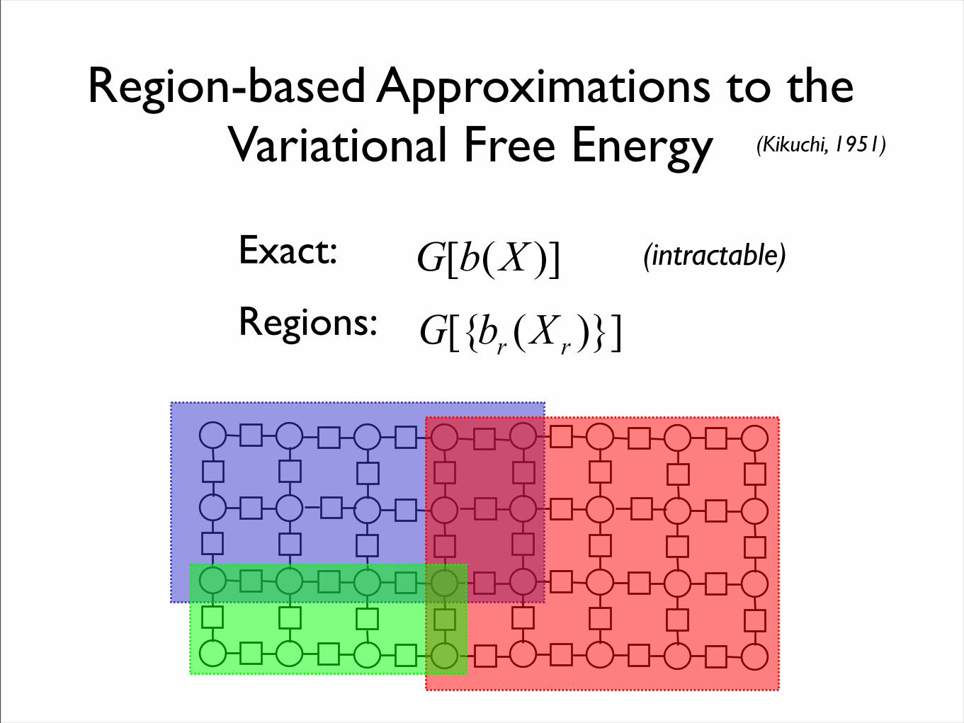
Region-based Approximations to the Variational Free Energy

Exact:

Regions:

(intractable)

(Kikuchi, 1951)

Defining a “Region” A region r is a set of variable nodes Vr and factor nodes

Fr such that if a factor node a belongs to Fr , all variable nodes neighboring a must belong to Vr . A region free energy can be naturally defined. The overall free energy will be the sum of the region free energies, weighted by their counting numbers.

Regions

Not a Region

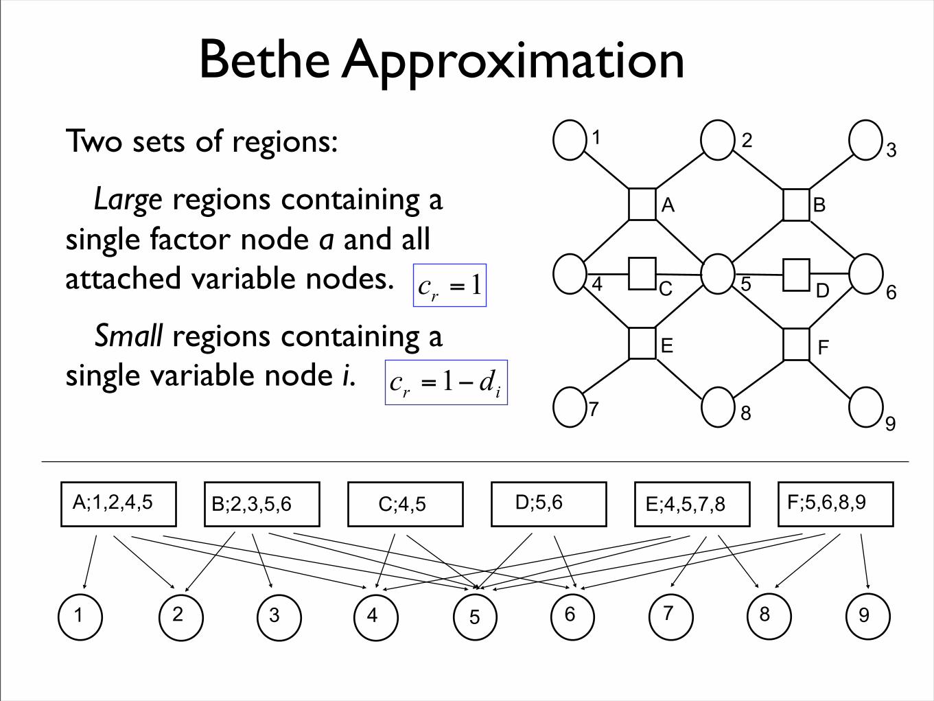
Bethe ApproximationTwo sets of regions:

Large regions containing a single factor node a and all attached variable nodes.

Small regions containing a single variable node i.

3

6

9

1 2

4 5

7 8

A B

C D

E F

A;1,2,4,5 B;2,3,5,6 C;4,5 D;5,6 E;4,5,7,8 F;5,6,8,9

1 2 3 4 5 6 7 8 9

bs =!

i

bi(xi) (13)

GBethe ="

a

"

Xa

ba(Xa) log#

ba(Xa)fa(Xa)

$+

"

i

(1! di)"

xi

bi log bi(xi) (14)

2

Bethe Free Energy

Minimizing the Bethe Free Energy, subject to the normalization and consistency constraints, gives a set of equations that is equivalent to the Belief Propagation message update rules!

Improving on BP• Generalized Belief Propagation: Using larger regions, construct a more

accurate region-based free energy, or equivalent message-passing algorithm. Particularly useful for factor graphs defined on a square lattice.

• Survey Propagation: Account for the possibility of many thermodynamic states by keeping a probability distribution over messages. Particularly useful for constraint-satisfaction problems.

• Loop Calculus: An expansion where the zeroth order term is BP, and the corrections can be systematically computed.

• Convexified Free Energies: approximations, with a unique global minimum which can be used to obtain rigorous lower bounds on the free energy.

• Expectation Propagation: an algorithm, with a different derivation but very close connections to Generalized Belief Propagation; it also can be used to derive message-passing algorithms for factor graphs with continuous variables.

Pointers to the Literature• “Information, Physics, and Computation,” M. Mézard and A. Montanari, Oxford University

Press, forthcoming--draft available online.

• “Factor Graphs and the Sum-Product Algorithm,” F.R. Kschischang, B.J. Frey, and H.-A. Loeliger, IEEE Trans. Info. Theory, 47:498-519, (2001).

• “Constructing Free Energy Approximations and Generalized Belief Propagation Algorithms,” J.S. Yedidia, W.T. Freeman, and Y. Weiss, IEEE Trans. Info. Theory, 51:2282-2312, (2005).

• “A New Class of Upper Bounds on the Log Partition Function,” M.J. Wainwright, T. S. Jaakkola, and Alan S. Willsky, IEEE Trans. Info Theory, 51: 2313-2335 (2005).

• “Structured Region Graphs: Morphing EP into GBP,” M. Welling, T. Minka, and Y.W. Teh, UAI (2005).

• “Survey Propagation: an Algorithm for Satisifiability,” A. Braunstein, M. Mézard, and R. Zecchina, Random Structures and Algorithms, 27: 201-226 (2005).

• “Loop Series for Discrete Statistical Models on Graphs” M. Chertkov and V. Chernyak, cond-mat/0603189, JSTAT P06009 (2006).

• and references in these papers and more recent papers by all these authors. (Apologies to all those I’ve neglected.)

belief propagation tutorialquestions • what is the most probable conﬁguration? • what is the...

Documents