beliefs and consumer search in a vertical industry

Economics Working Paper Series

Working Paper No. 1605

Beliefs and consumer search in a vertical industry

Maarten Janssen and Sandro Shelegia

March 2018

Beliefs and Consumer Search in a Vertical Industry∗

Maarten Janssen†and Sandro Shelegia‡

March 20, 2018

Abstract

This paper studies vertical relations in a search market. As the wholesale ar-

rangement between a manufacturer and its retailers is typically unobserved by con-

sumers, their beliefs about who is to be blamed for a price deviation play a crucial

role in determining wholesale and retail prices. The common assumption in the con-

sumer search literature is that consumers exclusively blame an individual retailer

for a price deviation. We show that in the vertical relations context, predictions

based on this assumption are not robust in the sense that if consumers assign just a

small probability to the event that the upstream manufacturer is responsible for the

deviation, equilibrium predictions are qualitatively different. For the robust beliefs,

the vertical model can explain a variety of observations, such as retail price rigidity

(or, alternatively, low cost pass-through), non-monotonicity of retail prices in search

costs, and (seemingly) collusive retail behavior. The model can be used to study a

monopoly online platform that sells access to final consumers.

JEL Classification: D40; D83; L13

Keywords: Vertical Relations, Consumer Search, Double Marginalization, Product

Differentiation, Price Rigidities

∗We have benefitted from comments by Natalia Fabra, Doh-Shin Jeon, Dmitry Lubensky, Jose-LuisMoraga-Gonzalez, Alexei Parakhonyak, Patrick Rey, Andrew Rhodes, Anton Sobolev, Chris Wilson andparticipants to the IV workshop on Consumer Search (Moscow) and seminars in Barcelona, Milan andParis, Toulouse, XXIX Jornadas de Economia Industrial 2014 and EARIE 2017. Shelegia acknowledgesfinancial support from the Spanish Ministry of Science and Innovation grant MINECO ECO2014-59225-P. Shelegia acknowledges financial support from the Spanish Ministry of Economy and Competitiveness,through the Severo Ochoa Programme for Centres of Excellence in RD (SEV-2015-0563).†Department of Economics, University of Vienna and State University Higher School of Economics.

Email: [email protected]‡Department of Economics and Business, Universitat Pompeu Fabra and Barcelona GSE. Email:

[email protected].

1

1 Introduction

In consumer search markets, the market power of firms depends on consumers’ willingness

to search. When at a firm, consumers compare the benefit of buying now with the expected

benefit of continuing to search. The expected benefit of search crucially depends on the

price consumers believe the next firm charges. As beliefs determine how consumers react

to price changes, they are important in determining how profitable price changes are.

If consumers are pessimistic about whether the next search will yield a good offer (low

price), they are more likely to accept the current offer, giving firms incentives to set higher

prices.

This basic insight is important in any search market, but – as we will argue in this

paper – it is particularly important in vertically related markets where a supplier (or

manufacturer) sells an input to firms (or retailers) who sell to final consumers searching

for good product matches and prices. One may think of a variety of product markets,

such as the ones for electronic products, where retailers’ marginal cost to a large extent

is determined by the wholesale price that is chosen by the manufacturer. In these envi-

ronments, the final retail price a consumer observes is the product of the input price set

by the manufacturer and the way the retailer reacts to that price. As consumers typically

do not know the wholesale arrangement between retailers and manufacturers, consumers

may ‘blame’ either the retailer or the manufacturer or both for any deviation from the

price they anticipated to observe. Consumers’ beliefs about retail prices that are not yet

observed may then depend on the retail prices consumers observe at the firm they are

visiting currently as consumers may reason that these prices move together in response

to the wholesale price that is set by the common manufacturer.

To focus on this key idea, we model the interaction between one monopoly input

supplier who offers a (possibly) non-linear contract to two independent retailers who

compete in a search market a la Wolinsky (1986). We then make two key contributions.

First, we make a methodological contribution by demonstrating that the behavior

of firms in vertically related markets critically depends on whom consumers blame for

deviations from equilibrium prices. In the literature following Wolinsky (1986),1 the

typical assumption is that if consumers observe an unexpected (i.e., non-equilibrium)

price, they believe that firms that are not yet visited sell at the equilibrium price. We

show that using this assumption in a vertical industry leads to predictions that are not

robust, in the sense that, if consumers believe that there is even an arbitrarily small chance

that the common supplier is responsible for an unexpected retail price they observe, then

the equilibrium is qualitatively different. In particular, we show that if consumers fully

1Starting from Anderson and Renault (1999), there is a wide range of recent papers that build onthe Wolinsky model. See, e.g., Anderson and Renault (2006), Bar-Isaac, Caruana and Cunat (2011),Armstrong, Vickers and Zhou (2009), Zhou (2014), and Armstrong and Zhou (2015), among others. Allthese papers employ what we will call in this paper the standard or typical assumption.

2

blame individual retailer for deviations from the equilibrium price, then a pure strategy

equilibrium does not exist if the search costs are intermediate, whereas for larger search

costs the market will partially break down in the sense that consumers who are unsatisfied

with their product match at the first firm drop out of the market rather than search

further. If consumers (at least partially) blame the monopoly supplier for observed non-

equilibrium prices, then a pure strategy equilibrium always exists and the supplier is

largely able to prevent the market breakdown.

Our second contribution is more substantial. We show that combining the vertical

relations literature with the search literature a la Wolinsky (1986) yields new explanations

for such diverse phenomena as price rigidities and other forms of low cost pass-through

rates, a non-cooperative explanation for seemingly collusive behavior at the retail level,

and non-monotonicity of retail prices in search costs.

To fully explain these results, it is convenient to first explain an intermediate result

regarding downstream market. In particular, there is a discontinuous drop in retail sales

(partial market break down) if search cost surpasses a threshold value. To understand

how this happens, it is important to relate the Wolinsky model to the Diamond Paradox

(Diamond, 1971). Diamond showed that with homogenous goods, for any positive search

cost, there will be no search beyond the first firm and all firms will charge the monopoly

price. As pointed out By Anderson and Renault (1999), Wolinsky solved the paradox by

introducing product differentiation, giving some consumers incentives to search. However,

when the search cost is sufficiently high and so prices are high, Wolinsky’s solution fails

because even consumers with very low utility draws are not willing to pay the search cost

to try their luck at a second firm if they expect prices to be high. As a result, when the

search cost exceeds a threshold, firms’ demand consists of first visits only which leads to

a demand drop because consumers discover fewer favorable matches. The existence of

such a search cost threshold, and the associated partial market breakdown has not been

explored in the search literature before. Without the interaction with an upstream firm,

this partial market breakdown is independent of the assumption concerning consumer

beliefs, but it plays an important role in explaining the non-robustness of the equilibrium

predictions under the assumption that consumers exclusively blame the individual retailer

they visit for deviations from the expected (equilibrium) price.

Using this intermediate result, we now explain that if consumers at least partially

blame the monopoly supplier for deviations from an anticipated retail price, the retail price

is non-monotonic in search cost. For relatively small search costs, the price is increasing

in search cost (as in the standard model). At intermediate values of the search cost,

firms charge prices that are equal to the reservation utility. Since the latter is decreasing

in the search cost, so are prices.2 Overall, in this range the price is hump-shaped in

2This inverse relationship between search cost and prices is unlike the earlier contributions with thesame conclusion. In Janssen, Moraga-Gonzalez and Wildenbeest (2005), the search cost changes the

3

search cost. Interestingly, at the maximum, both firms set the price that a monopolist

selling both goods would set. This price is higher than the single-good monopoly price

because a joint profit maximization internalizes demand externalities between the two

(substitute) goods. Thus, for intermediate search costs when consumers blame a common

supplier for unexpected retail prices a fully collusive outcome results even though firms

act non-cooperatively!

Another way in which this intermediate result is used is in demonstrating that re-

tail prices may be sticky relative to changes in the supplier’s wholesale price (or other

components of retailers’ marginal cost). Fixing the search cost, we may investigate how

the downstream equilibrium changes as the downstream marginal cost increases. This

perspective is important in vertically related markets where the input price set by the

supplier plays the key role. Under the typical assumption where consumers exclusively

blame individual retailers for unexpected prices, the final consumer price is always in-

creasing in a firm’s marginal cost. When consumers hold the supplier at least partially

responsible for unexpected prices, there is an intermediate level of the retailers’ marginal

cost where the retail price equals the reservation utility, and because the reservation util-

ity does not depend on the marginal cost, neither does the retail price. So, under these

robust consumer beliefs, the retail price is first increasing in retailers’ cost, then constant,

and then increasing again.

Equipped with these results in the downstream market, we can investigate the verti-

cally related market where retailers’ cost is partially determined by an upstream supplier.

Under the typical assumption where consumers exclusively blame the individual retailer

they visited for setting an unexpected price, the equilibrium structure is as follows. For

low search costs, the manufacturer sets a wholesale price such that retail prices are smaller

than the reservation utility and consumers search beyond the first firm if the utility draw

at the first firm they visited was low. For high search costs, the supplier’s optimal price

is such that retail prices will be higher than the reservation utility, consumers do not

search beyond the first firm and (despite the possibility of offering non-linear wholesale

contracts) a classic double-marginalization outcome results. For intermediate search cost,

a pure strategy equilibrium does not exist.

For any other belief, where consumers assign a positive probability to the event that

the common supplier is responsible for an unexpected price change, market outcomes

are very different. The behavioral patterns we have already discussed (price rigidities,

seemingly collusive behavior, non-monotonicity in search cost) remain, and get even fur-

ther strengthened when we include the optimal pricing behavior of the supplier. As the

supplier’s indirect demand consists of the demand of both retailers, the supplier has an

composition of heterogeneous consumers and may result in lower prices at higher search cost. In Zhou(2014) consumers search for multiple products. In this environment, products are search complementsand if the search cost increases, firms may compete more intensely to prevent consumers searching further.

4

incentive to induce the retailers to charge the joint profit maximizing prices. As he affects

the retail prices through the choice of the per unit wholesale price, he is also in partial

control of the beliefs consumers have. Given this incentive and the ability to implement

it, he sets an input price that maximizes the profits of the vertical structure (and extracts

all the profits with the fixed fee). For larger search cost, to avoid market breakdown, he

will make sure that the retail prices are not larger than the reservation utility. Retailers

would not by themselves do so because they are not interested in encouraging their own

consumers to search further. The upstream supplier does care because more search means

results in higher total demand. The fact that beliefs move with prices conveniently pre-

vents the upstream firm from deviating to inducing higher retail prices because consumers

update their beliefs and stop searching. To the best of our knowledge, there is no other

paper where a firm proactively seeks to prevent the Diamond Paradox from arising.

There is a small, but growing literature that combines consumer search with verti-

cal relations. Janssen and Shelegia (2015) demonstrates that the fact that wholesale

price arrangements are unknown to consumers has an important qualitative and large

quantitative impact on market outcomes. They use the Stahl (1989) search model for

homogeneous goods to make this point. Garcia, Janssen and Honda (2017) extend the

analysis to multiple manufacturers and show that the vertical search model can explain

the frequently observed phenomenon of bimodal retail prices. Lubensky (2017) introduces

vertical relations in the model of Wolinsky (1986) to study the role of recommended retail

prices, while Asker and Bar-Isaac (2017) focus on the impact of another vertical restraint,

namely minimum advertised prices (MAPs).

The paper is also related to the nascent literature on competition on platforms, like

amazon.com or booking.com (see, e.g., Wang and Wright (2017)). That literature studies

the interaction between the fees platform(s) set to allow firms sell through their website

and the pricing policies of the firms themselves in a world where consumers search for

products on the platform(s), but may also buy from the firms directly. An important

policy debate in this regard is on whether most favored nation clauses lead to higher

prices or not. In terms of this literature, our paper can be re-interpreted in the following

way. The input provider is the platform and the essential input he provides is the access to

consumers. In our paper, the firms cannot sell to consumers outside of the platform. This

captures the fact that for certain products in the online world many sellers are not Known

to consumers and therefore firms will not be able to sell to them without being listed on

the platform.3 As we have a monopoly supplier, we do not model platform competition,

unlike e.g., Karle, Peitz and Reisinger (2017), but what we bring to the literature is the

3? review evidence by the UK’s Competition and Market Authority (CMA) showing thatprice comparison websites have heavily invested in establishing a brand name and that depend-ing on the product, many consumers are loyal to a platform and search only there. See, e.g.,https://assets.publishing.service.gov.uk/media/58e224f5e5274a06b3000099/

dcts-consumer-research-final-report.pdf.

5

focus on consumers not knowing the pricing arrangement between firms and the platform

and how their ignorance affects search behavior and, as a consequence, the pricing policies

of firms and platform. The above literate has not focused on this issue.4

The rest of the paper is organized as follows. In Section 2 we set up the model, discuss

the equilibrium concept used and explain the search and demand behavior of consumers

and how this depends on the information consumers possess and the beliefs they hold.

In Section 3 we analyze the downstream market and show how firms’ pricing depends

on whom consumers hold responsible for unexpected price observations. In Section 4, we

provide the full equilibrium analysis by analyzing the optimal behavior of the supplier and

show what type of equilibrium predictions result for different beliefs. Section 5 concludes.

Proofs are contained in the Appendix.

2 The Model and Equilibrium Concept

The retail side of the model we study follows Wolinsky (1986). There are two firms, 1

and 2, who have a common cost c per unit. The firms transform the input into a final

differentiated good, using a one-for-one technology. There is a unit mass of consumers

per firm. Utility to a consumer from buying the good at firm i is vi. This utility is drawn

from the distribution function G(v), with the corresponding density g(v) , which is the

same for both firms and defined over the (possibly infinite) interval [v, v]. As is standard

in the literature (see e.g., Anderson and Renault (1999)), we require that 1 − G(v) is

log-concave. A consumer’s valuation for firm 1’s product is independent of his valuation

for firm 2’s product. A consumer visits one of the firms at random and finds out vi and pi.

After observing the match value vi and the price pi the consumer decides whether or not

to visit the second firm. If she does so, she makes her purchase to get the best available

surplus vi−pi, provided that it exceeds zero, the outside option. We assume that the first

visit is free.5 The second visit is costly, and the cost is denoted by s. If after visiting the

first firm, a consumer decides to search the second firm, she can always go back to the

first firm at no additional cost (free recall). The above set-up is common to all consumer

search models based on Wolinsky (1986).

We now turn to the monopolist supplier. The supplier offers both downstream firms

a common two-part tariff consisting of a unit wholesale price w and a fixed fee F . Firms

have to spend t to transform the homogenous input into the differentiated output they

sell, so that each firm’s marginal cost is given by c = w + t. We can interpret the two

levels of the supply chain in different ways: two firms with a common supplier, or two

retailers selling a product of the same manufacturer, or two firms buying access to final

4Wang and Wright (2017) assume that the fee charged by the platform is known to consumers.5Most of our results continue to hold if the first search is costly. There is a slight difference in results

when s (or t -see below) is large and in Section 4 we comment on how the results would change if thefirst search is also costly.

6

consumers via a monopoly platform. Accordingly, we can interpret t as the marginal cost

of transformation, or a retailer’s shelving cost or a unit sales tax, or the firms’ own cost

of production (on top of the access fee to consumers) or a combination of these. We use

these interpretations interchangeably.

As consumers do not know firms’ prices (before observing them), it is natural to also

assume that consumers do not observe the wholesale contract.6 Note that the final price

consumers observe is the end result of the wholesale price set by the supplier and the

firm’s pricing strategy (a price for any given input price). After observing an out-of-

equilibrium retail price, consumers may hold any belief regarding who has deviated from

the equilibrium path. They may put full responsibility on either the downstream firm or

the upstream firm, or they may hold both parties partly responsible. If they believe that

the firm they visited has deviated, then they aught to think that the other downstream

firm’s price is unchanged. At the other extreme, if they believe that the supplier has

charged a different wholesale price affecting all firms, then they may expect the other

downstream firms to react in the same way to the upstream firm’s deviation.7

To study the role of consumer beliefs in sustaining market outcomes, we introduce the

following notation. Denote by p∗ the equilibrium price a consumer expects to encounter

at both stores in the symmetric equilibrium. If a consumer, on his first search, encounters

an out-of-equilibrium price pi 6= p∗, he has to form a (point) belief pej of the price set by

firm j that has not been yet visited. If the consumer only ‘blames’ the firm he has visited

first for the deviation, then he believes that the firm not yet visited has set pej = p∗.

On the other hand, if the consumer blames the upstream firm, then he believes that the

firm not yet visited sets pej = pi. In general, if the consumer holds both parties partly

responsible, their beliefs may be a convex combination of the previous two cases, i.e.,

pej = αp∗ + (1− α)pi for a given α ∈ [0, 1]. Any other relationship between pej and pi and

p∗ may hold, provided that for pi = p∗ we have pej = p∗, but in this paper, for expositional

simplicity, we focus on the linear form provided here.8

The equilibrium notion we employ is formally defined as follows.

Definition 1. For a given t, a symmetric perfect Bayesian equilibrium is a wholesale

6In the context of the Stahl (1989) sequential search model for homogeneous goods, Janssen andShelegia (2015) focus on the comparison of markets where consumers observe the wholesale price andmarkets where they do not observe the wholesale price. We focus here on the role of consumer beliefs whereconsumers do not observe the wholesale price. In the earlier version of this paper we also considered thevertical relations model where the wholesale price is observed by consumers, and confirmed Janssen andShelegia’s finding that, holding beliefs the same, prices are higher when the wholesale price is unobserved.

7Without vertical relations, the consumer search literature implicitly or explicitly uses “passive” be-liefs. In terms of the notation to be introduced shortly, passive beliefs imply pej is independent of pi(corresponding to α = 1). The vertical contracting literature (see, e.g., Hart et al. (1990) and McAfeeand Schwartz (1994)) also considers “symmetric” beliefs, which in our setting can be described as pej = pi:consumers who first visit firm i believe that firm j charges the same price as i.

8As will become apparent later, most of our results depend on the derivative of pej with respect to piaround pi = p∗, which in the linear formulation is simply equal to 1− α.

7

contract (w∗, F ∗), a contract acceptance strategy and a retail pricing strategy p∗(c) for the

firms, and a reservation utility r(p) such that

1. The supplier chooses (w,F ) so as to maximize its profit given the contract acceptance

strategy and the pricing strategy p∗(c) of the firms, and consumers’ reservation utility

r(p);

2. Each firm i decides to accept or reject (w,F ). If the firm accepts, it chooses pi(c) =

p∗(c) to maximize its expected profit given the pricing strategy p∗(c) of the other firm

and consumers’ reservation utility r(p);

3. Consumers follow an optimal reservation search rule given their beliefs, the match

value vi and the price pi they observe at firm i;

4. Consumers’ common belief about the price set by the firm that is not yet visited, pej,

given the price they have observed, pi, satisfies pej = αp∗(c∗) + (1 − α)pi for some

α ∈ [0, 1].

It is important to understand why we focus on the duopoly case. First, focusing on

duopoly allows us to avoid the issue of belief formation after two different prices have

been observed. As there is no obvious way to do this, the focus on duopoly simplifies the

analysis considerably. In particular, with two firms, a consumer can update her belief only

once (after visiting the first firm) making belief formation relatively straightforward. For

three or more firms, it may be the case that, after having searched two firms, a consumer

has observed two different prices and needs to update his belief in order to decide whether

to continue to search or not. Second, regardless of how subsequent beliefs are formed,

the issues we uncover in the duopoly model are still relevant because they concern the

first search. In fact, by virtue of the fact that consumers are more, and often much more,

likely to search once rather than to search two or more times, our analysis is of first-order

relevance even in oligopoly models.

2.1 Consumer Behavior

Given that the wholesale contract is unobserved by consumers (who move last), there

are no subgames of the model that can be analyzed on their own. However, before

analyzing the supplier’s behavior, it is still useful to first analyze the behavior of consumers

and downstream firms for a given input price w. In this subsection, we specify how the

downstream firms’ demand depends on consumer beliefs.

Consider a consumer who visits firm i. A reservation utility strategy is a strategy where

the consumer continues to search if the utility drawn is below a certain threshold, and stops

if the utility exceeds this threshold. This threshold depends on the utility realization, firm

i’s price and the belief about firm j’s price. Before finding it, we determine the reservation

8

utility r, a utility level at which a consumer is indifferent between searching the second

firm, or accepting r, assuming that both firms charge equal prices. The reservation utility

r is the solution to ∫ v

r

(v − r)g(v) dv = s, (1)

if the solution exists, and is equal to r = v if it does not.

The threshold utility level is then simply computed as r plus the (expected) price

difference. Formally, a consumer who draws vi and pi prefers to search rather than to

accept the current offer if

vi < r + (pi − pej).

The consumer has, however, a third option, namely not to continue to search and not to

buy. For the consumer to continue to search we need an additional condition to hold,

namely that her reservation utility exceeds the price expected at the other firm, r ≥ pej ;

otherwise the expected benefit from search is negative and the consumer does not search

beyond the first firm.

Given the optimal search behavior above, we can write down firm i’s demand. As the

expression below shows this demand differs from the standard expression in the literature

following Wolinsky (1986) in several respects. The expression allows firm i, whose demand

is being computed, to set a price pi, which may differ from all of the following: (i) the

price pj of its rival, (ii) the belief pei consumers who make their first visit to firm j hold

about the price of firm i, and (iii) the belief pej consumers who make their first visit to firm

i first hold about firm j’s price. When deriving the equilibrium price, the search literature

based on the Wolinsky model sets all pj, pej and pei equal to the candidate equilibrium price

p∗. We need to isolate all four because in the vertical relations model upon a deviation

by the supplier from w∗, if firm i is itself deciding whether to deviate or not, it may find

itself in a situation where all four terms are different from each other.

Firm i’s demand is given by

qi(pi, pj, p∗) = (1−G(pi + max{r − pej , 0})) +

∫ pi+max{r−pej ,0}

pi

G(pj − pi + v)g(v)dv

+

[G(r − pei + pj)(1−G(r − pei + pi)) +

∫ r−pei +pi

pi


]· Ir≥pei .

(2)

The first term is the demand from consumers who visit firm i and buy outright because

their utility draw is higher than the threshold r−pej +pi. The second term is the demand

from those consumers who first visit firm i, draw a utility below r − pej + pi, visit firm j,

but come back and buy from firm i. The first two groups of consumers only search when

r ≥ pej , and otherwise the firm’s demand from them is simply 1−G(pi).9 The first term

in square brackets is the demand from consumers who first visit firm j, draw a value vj

9This is the reason why we write max{r − pej , 0}.

9

that is lower than the threshold value r − pei + pj, decide to visit firm i, find a utility

draw vi that is higher than r − pei + pi and buy from firm i. The second term inside

the square brackets is similar to the first one, but accounts for those consumers who first

visit firm j, decide to search firm i, also draw a relatively low value at firm i, but still

buy at firm i as that price/product offer is better than that offered by firm j. These two

terms are multiplied by an indicator function Ir≥pei that is equal to 1 when r ≥ pei . In the

opposite case consumers arriving first to firm j never continue to search, and thus they

never purchase from firm i.

The demand expression for firm i is illustrated in Figure 2 in (vI , vj) space for the

case where r ≥ pek, k = i, j. Area A corresponds to the first term in (2) which refers to

consumers who arrive at firm i first, draw vi above r − pi + pej and buy outright. Area B

corresponds to consumers who arrive at firm i first but continue to search because their

utility draw vi is smaller than r− pi + pej and then come back to buy because their utility

draw at firm j is even worse (the second term in (2)). Areas C and D correspond to

consumers who first visit firm j, draw a utility level vj that is smaller than r − pj + pei ,

continue to search firm i and purchase there as their utility at firm i is higher than pi and

higher than the utility at firm j. Note that consumer beliefs affect who searches, but not

whether consumers buy or not.

A

B

vj

vi

pi

pj

pi � pj

v j+

p i� p j

pi

pjvj

vi

v j+

p i� p j

pi � pj

i) ii)

C

D

r + pi � pej r + pi � pe

i

r + pj � peir + pj � pe

j

Figure 1: Figures i) and ii) depict consumers who buy from firm i after having made afirst visit to firm i and firm j, respectively.

3 Downstream Behavior

In this section we study how the downstream pricing behavior depends on the wholesale

price w. This is important for several reasons. First, as we will show, the downstream

behavior is interesting in its own right. Namely, low cost pass through and seemingly

10

collusive behavior emerge as the result of this isolated analysis of the downstream level.

Second, to determine the overall equilibrium for the vertical model, when choosing the

wholesale arrangement (w∗, F ∗) optimally, the supplier needs to consider how retailers

would react to deviations from the equilibrium wholesale arrangement.

Thus, consider the downstream market for a given input price w and consumers that

have a prior belief (before searching any firm) that the symmetric equilibrium downstream

price is p∗. (This belief corresponds to the equilibrium wholesale price w∗). Each firm

observes (w,F ) and has to decide whether to accept this wholesale contract, and if so,

what price to set. If they accept, they will set a price p(w) to sell to consumers. At this

stage we allow both that p(w) 6= pi 6= p∗ and that w 6= w∗, so that once we want to study

the supplier’s optimal pricing strategy we can calculate the supplier’s deviation payoff for

any w 6= w∗. As the outside option of a downstream firm is not to sell anything, it will

accept any contract if the expected profit of setting p(w) is larger than or equal to 0,

provided that the other players acts according to the equilibrium.

For a given expected (equilibrium) downstream price p∗ by consumers and a wholesale

contract (w,F ) we define a downstream market equilibrium as follows. Note that as

consumers do not observe the same wholesale contract (w,F ), the downstream behavior

cannot be analyzed as a separate subgame of the whole game. Still, and this will be

important in the next section, as both downstream firms observe (w,F ) there is some

strategic interaction between them. To clarify that consumers do not observe the wholesale

contract, this strategic interaction is conditional on consumer beliefs, represented by p∗.

Definition 2. Fix α and s. For a given expected downstream price p∗ and a wholesale

contract (w,F ), a symmetric downstream market equilibrium is a function p(w) and an

acceptance decision such that (i) p(w) is the optimal pricing decision given that the other

firm chooses the same price, the wholesale contract is given by (w,F ) and demand is given

by (2) and (ii) each firm makes nonnegative profits given both firms choose p(w).

In this section, we will derive the symmetric equilibrium price p(w) which may be

different from p∗ if w 6= w∗. To this end, consider firm i who is contemplating to charge pi

when the other firm is expected to charge the equilibrium price p(w). In order to facilitate

this derivation, we will first define for α < 1

p ≡ r − αp∗1− α

as the threshold price such that when pi = p we have pej(pi) = r. Since∂pej(pi)

∂pi= 1−α,

for α < 1 if pi exceeds p consumers who first visit firm i will not search further if their

match value with firm i is too low. For future reference, note that p is (weakly) decreasing

in s. This is because the higher the search cost, the lower the reservation utility, and

therefore the lower is the threshold price r at which consumers stop searching. The

11

case where α = 1 is special and in the next section we show that taking the upstream

manufacturer into account, the equilibrium predictions of the vertical model for α = 1

are not robust and they differ in important qualitative ways from the model where α < 1.

For now, to characterize the downstream equilibrium laying the groundwork for the next

section, we will define p to be −∞ when p∗ > r and +∞ for p∗ ≤ r for the case where

α = 1.

For a general utility distribution, it is difficult to prove a downstream equilibrium

exists. The difficulty is that for general beliefs p∗ and for 0 < α < 1 one has to evaluate

the profit function at different values of G(.). The next Proposition shows that equilibrium

existence is not an issue if G(.) is uniform.

Proposition 1. If the utility distribution G(v) is uniformly distributed on [0, 1], then a

symmetric downstream equilibrium exists and is unique.

The proof shows that the profit function πi(pi, pj, p∗) = qi(pi, pj, p

∗)(pi − c) is concave

for pi p. It is also overall concave because the

left derivative of the profit function at pi = p strictly exceeds the right derivative at the

same point implying there is a kink in the profit function at p. The proof shows that

this latter property holds true independently of the uniformity assumption. Thus, the

uniform distribution is only used to show the (quasi-)concavity on both sides of the kink.

In the rest of the paper we assume that G(.) is such that a symmetric equilibrium exists

and is unique. From the above proposition we know that this is the case for the uniform

distribution.

In general, there are three possibilities for the symmetric equilibrium price p(w): (i)

p(w) p and each firm is a local monopolist

with demand 1−G(pi).

Let us start characterizing the first case. If demand is as in (2), then for any w the

equilibrium price in the downstream market is characterized by the following condition

(where we omit the dependence of p on w):

p− c =qi(p, p, p

∗)

− ∂qi∂pi

(p, p, p∗).

This is a standard pricing condition for a firm with demand qi and marginal cost c.

What is worth commenting on is that both the demand, and its derivative with respect

to i’s own price are evaluated at pi = pj = p, and the initial belief of consumers is allowed

to be different from both. After some simple algebra, the above condition transforms into

p− c =1−G(p)2

2∫ α∆p+r

pg(v)2 dv + 2g(p)G(p) + α(1−G(α∆p+ r))g(α∆p+ r)

, (3)

12

where ∆p = p − p∗. In the overall equilibrium of the vertical industry, the price

difference ∆p is zero. For future reference, the solution to (3) will be denoted by p.

In the standard model where α = 1 and ∆p = 0, this pricing rule induces the same

price as in Wolinsky (1986), but in general, it is different in two respects. First, the

candidate equilibrium price is smaller than in the standard model for any α < 1. Second,

the equilibrium price is decreasing in ∆p, and therefore is increasing in p∗. Thus, the

lower is the price that consumers expect before embarking on search, the lower is the

equilibrium price. This is intuitive in that if consumers are more optimistic about finding

lower prices in the market, they are more willing to search and thus firms are forced to

charge lower prices.

It is trivially true that the solution to (3) is increasing in c, so for p < p to hold, we

need that c is sufficiently low. The threshold, denoted by c1(p∗), is found by substituting

p = p into (3) and solving for c, which gives

c1(p∗) ≡ p− 1−G(p)2

(α + (2− α)G(p))g(p).

If c < c1(p∗), then provided that firm j charges pj = p(w), firm i will maximize the

section of its profits to the left of p by also charging pi = p(w). In fact, it cannot do

better with any pi > p.

Now consider case (iii) where p(w) > p, i.e., if the match value at the first firm is low,

consumers do not search beyond the first firm. Each firm is then effectively a monopolist

facing demand 1−G(p), and so the equilibrium price p(w) = pMc where pMc is the standard

monopoly price for marginal cost c that solves

pMc = c+1−G(pMc )

g(pMc ). (4)

The situation is now reversed. If firm j charges pj = pMc , firm i will maximize the

section of its profits to the right of p by also charging pi = pMc . This situation occurs

when p(w) = pMc > p which holds when c exceeds c2(p∗) found by substituting p in (4)

for pMc and solving for c. This yields

c2(p∗) ≡ p− 1−G(p)

g(p).

We can now proceed to case (ii) by noting that c2(p∗) > c1(p∗) for α < 1.10 When

c ∈ (c1(p∗), c2(p∗)), if firm j charges pj = p, firm i also maximizes its profits with pi = p.

As explained, this is because now the kink at p is the maximizer of the overall profits.

Given the above discussion, we characterize the symmetric downstream equilibrium

price p as follows.

10Note that c1(p∗)→ c2(p∗) if α→ 1, so the region between the two threshold values disappears.

13

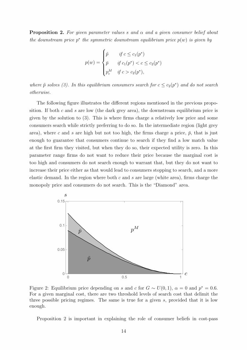
Proposition 2. For given parameter values s and α and a given consumer belief about

the downstream price p∗ the symmetric downstream equilibrium price p(w) is given by

p(w) =

p if c ≤ c1(p∗)

p if c1(p∗) < c ≤ c2(p∗)

pMc if c > c2(p∗),

where p solves (3). In this equilibrium consumers search for c ≤ c2(p∗) and do not search

otherwise.

The following figure illustrates the different regions mentioned in the previous propo-

sition. If both c and s are low (the dark grey area), the downstream equilibrium price is

given by the solution to (3). This is where firms charge a relatively low price and some

consumers search while strictly preferring to do so. In the intermediate region (light grey

area), where c and s are high but not too high, the firms charge a price, p, that is just

enough to guarantee that consumers continue to search if they find a low match value

at the first firm they visited, but when they do so, their expected utility is zero. In this

parameter range firms do not want to reduce their price because the marginal cost is

too high and consumers do not search enough to warrant that, but they do not want to

increase their price either as that would lead to consumers stopping to search, and a more

elastic demand. In the region where both c and s are large (white area), firms charge the

monopoly price and consumers do not search. This is the “Diamond” area.

0 0.5 10

0.05

0.1

0.150 0.5 1

0

0.05

0.1

0.15

c

s

p pM

p

Figure 2: Equilibrium price depending on s and c for G ∼ U(0, 1), α = 0 and p∗ = 0.6.For a given marginal cost, there are two threshold levels of search cost that delimit thethree possible pricing regimes. The same is true for a given s, provided that it is lowenough.

Proposition 2 is important in explaining the role of consumer beliefs in cost-pass

14

0 0.6

0.5

0.65

0.8

p

cc1(p

⇤) c2(p⇤)

pMc

pIMc

p

p1

p0

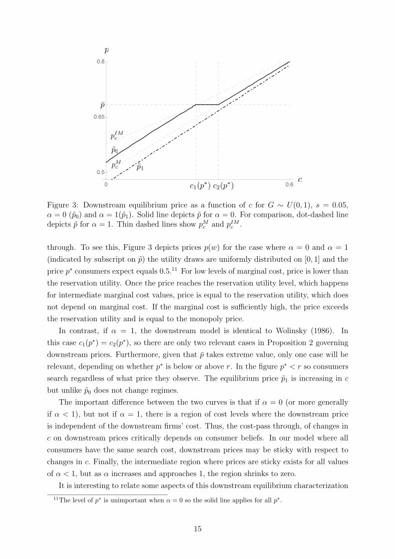
Figure 3: Downstream equilibrium price as a function of c for G ∼ U(0, 1), s = 0.05,α = 0 (p0) and α = 1(p1). Solid line depicts p for α = 0. For comparison, dot-dashed linedepicts p for α = 1. Thin dashed lines show pMc and pIMc .

through. To see this, Figure 3 depicts prices p(w) for the case where α = 0 and α = 1

(indicated by subscript on p) the utility draws are uniformly distributed on [0, 1] and the

price p∗ consumers expect equals 0.5.11 For low levels of marginal cost, price is lower than

the reservation utility. Once the price reaches the reservation utility level, which happens

for intermediate marginal cost values, price is equal to the reservation utility, which does

not depend on marginal cost. If the marginal cost is sufficiently high, the price exceeds

the reservation utility and is equal to the monopoly price.

In contrast, if α = 1, the downstream model is identical to Wolinsky (1986). In

this case c1(p∗) = c2(p∗), so there are only two relevant cases in Proposition 2 governing

downstream prices. Furthermore, given that p takes extreme value, only one case will be

relevant, depending on whether p∗ is below or above r. In the figure p∗ < r so consumers

search regardless of what price they observe. The equilibrium price p1 is increasing in c

but unlike p0 does not change regimes.

The important difference between the two curves is that if α = 0 (or more generally

if α < 1), but not if α = 1, there is a region of cost levels where the downstream price

is independent of the downstream firms’ cost. Thus, the cost-pass through, of changes in

c on downstream prices critically depends on consumer beliefs. In our model where all

consumers have the same search cost, downstream prices may be sticky with respect to

changes in c. Finally, the intermediate region where prices are sticky exists for all values

of α < 1, but as α increases and approaches 1, the region shrinks to zero.

It is interesting to relate some aspects of this downstream equilibrium characterization

11The level of p∗ is unimportant when α = 0 so the solid line applies for all p∗.

15

to the literature on sticky prices and incomplete cost pass-through. Starting with the

seminal contributions by Sheshinski and Weiss (1977), Akerlof and Yellen (1985a,b) and

Mankiw (1985), there is a large literature that explains why firms do not adjust prices

following cost shocks assuming an exogenous cost of price adjustment, the menu cost. Our

model generates price stickiness without assuming menu cost. Instead, prices are sticky

because, for a range of marginal costs, firms find it optimal to set prices equal to the

consumers’ reservation utility that is independent of marginal cost. Sherman and Weiss

(2015) empirically find that retailers in the Shuk Mahane Yehuda market in Jerusalem

do not react to cost changes. They explain this finding with a dynamic model where

consumers are not informed about the cost and do not adjust their expectations about

prices charged by other retailers. In this world, if retailers were to increase their prices

consumers would walk away to the next store. Compared to their paper, we have a static

model with product differentiation where beliefs are endogenously specified. Cabral and

Fishman (2012) have also proposed a search theoretic foundation for price stickiness.

Their framework relies, however, on some stickiness in retailers’ cost and they show that

consumer search may lead to retail prices that are even stickier. Our Proposition 2 does

not rely in any way on stickiness of retailers’ cost. The result that prices are fully rigid

does depend, however, on the assumption that all consumers have identical search costs.

If search costs are heterogeneous (see, also, Moraga-Gonzalez, Sandor and Wildenbeest

(2017)), but the search cost distribution is concentrated around a certain value, prices will

be “almost” sticky, and we would obtain a search theoretic explanation for incomplete

cost pass-through (Weyl and Fabinger (2013)).

One can also describe the results on downstream pricing in relation to search cost s

for a given marginal cost c. It is clear from Figure 3, but also from a close inspection of

the conditions in Proposition 2, that for a given c, there are two threshold levels of s,

whereby if s is smaller than the smallest threshold the price is p, if it is in between the

two thresholds the price is p, and if it is above the highest of the two threshold values,

the price is pMc . The next corollary restates proposition 2 for a given c by varying s. To

this end, let s1(p∗) denote the search cost such that c = p − 1−G(p)2

(α+(2−α)G(p))g(p), where r

(implicitly presented through its impact on p) depends on s, and is strictly decreasing in

s. Similarly, s2(p∗) solves c = p− 1−G(p)g(p)

.

Corollary 3. For given parameter values c and α and a given consumer belief about the

downstream price p∗, there exist s1(p∗) and s2(p∗) defined above, with s1(p∗) ≤ s2(p∗),

such that

p =

p if s ≤ s1(p∗)

p if s1(p∗) < s ≤ s2(p∗)

pMc if s > s2(p∗),

Figure 4 illustrates corollary 3 emphasizing the role of consumer beliefs again. If α = 1,

16

there are two cases as s1 = s2.12 If s is small, the price is smaller than the monopoly

price and increasing in s. For larger values of s, firms charge the monopoly price which is

independent of s. For α = 0 (and any α < 1) there are three cases again. For low search

costs, the price is increasing in the search cost and larger than when α = 1, but still small

enough so that consumers continue to search if they encountered a low match value on

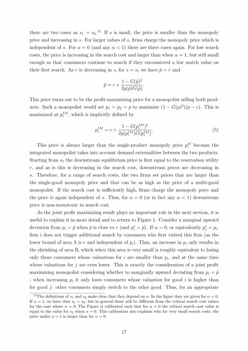
their first search. As r is decreasing in s, for s = s1 we have p = r and

p = c+1−G(p)2

2g(p)G(p).

This price turns out to be the profit-maximizing price for a monopolist selling both prod-

ucts. Such a monopolist would set p1 = p2 = p to maximize (1 − G(p)2)(p − c). This is

maximized at pIMc , which is implicitly defined by

pIMc = c+1−G(pIMc )2

2g(pIMc )G(pIMc ). (5)

This price is always larger than the single-product monopoly price pMc because the

integrated monopolist takes into account demand externalities between the two products.

Starting from s1 the downstream equilibrium price is first equal to the reservation utility

r, and as is this is decreasing in the search cost, downstream prices are decreasing in

s. Therefore, for a range of search costs, the two firms set prices that are larger than

the single-good monopoly price and that can be as high as the price of a multi-good

monopolist. If the search cost is sufficiently high, firms charge the monopoly price and

the price is again independent of s. Thus, for α = 0 (or in fact any α < 1) downstream

price is non-monotonic in search cost.

As the joint profit maximizing result plays an important role in the next section, it is

useful to explain it in more detail and to return to Figure 1. Consider a marginal upward

deviation from pi = p when p is close to r (and pei = p). If α = 0, or equivalently pej = pi,

firm i does not trigger additional search by consumers who first visited this firm (as the

lower bound of area A is r and independent of pi). Thus, an increase in pi only results in

the shrinking of area B, which when this area is very small is roughly equivalent to losing

only those consumers whose valuations for i are smaller than pi, and at the same time

whose valuations for j are even lower. This is exactly the consideration of a joint profit

maximizing monopolist considering whether to marginally upward deviating from pi = p

- when increasing pi it only loses consumers whose valuation for good i is higher than

for good j: other consumers simply switch to the other good. Thus, for an appropriate

12The definitions of s1 and s2 make clear that they depend on α. In the figure they are given for α = 0.If α = 1, we have that s1 = s2, but in general these will be different from the critical search cost valuesfor the case where α = 0. The Figure is calibrated such that for α = 0 the critical search cost value isequal to the value for s2 when α = 0. This calibration also explains why for very small search costs, theprice under α = 1 is larger than for α = 0.

17

0 0.2

0.4

0.5

0.6

0.7

s1(p⇤) s2(p

⇤)s

pIMc

pMc

p

p1

p0

Figure 4: Downstream equilibrium price as a function of s for G ∼ U(0, 1), c = 0, andp∗ = 0.5. Solid line depicts p for α = 0. For comparison, dot-dashed line depicts p forα = 1.

choice of s, firms act as if they are jointly maximizing profits. It is surprising that a

”collusive” outcome is achieved via consumer beliefs, while firms act independently, given

these beliefs.

4 Full Equilibrium Analysis

With two-part tariffs, the upstream manufacturer maximizes total vertical industry profit

subject to consumers’ search behavior. In particular, conditional on consumers searching,

the upstream firm would like to induce downstream firms to charge pIMt . This is the

integrated monopoly price for two substitutes when the downstream marginal cost is t.

It is clear that this equals the joint downstream profit maximizing price given the true

marginal cost of the manufacturer (which is normalized to 0).

When the search cost s is small enough such that pIMt ≤ r, the upstream firm can

safely induce pIMt by charging an appropriate wholesale price w and then extracting all of

the downstream profits through F . The exact level of w∗ and F ∗ depends on s, t and α.

In particular, the upstream firm has to set w∗ such that p(w∗) = pIMt for p = p∗ and then

set F ∗ = (1−G(pIMt )2)(pIMt −c∗). Interestingly, even if s = 0, the upstream manufacturer

needs to charge w∗ > 0 as by themselves the downstream firms do not take into account

the positive externality of a price increase on the demand of the substitute, and the

positive effect this has for the manufacturer (as he sells anyway whether a consumer buys

from one or the other retailer, and can set a higher fixed fee if retailers make more profits).

In order to find w∗, we have to take (3) and impose p(w∗) = p∗. The resulting pricing

18

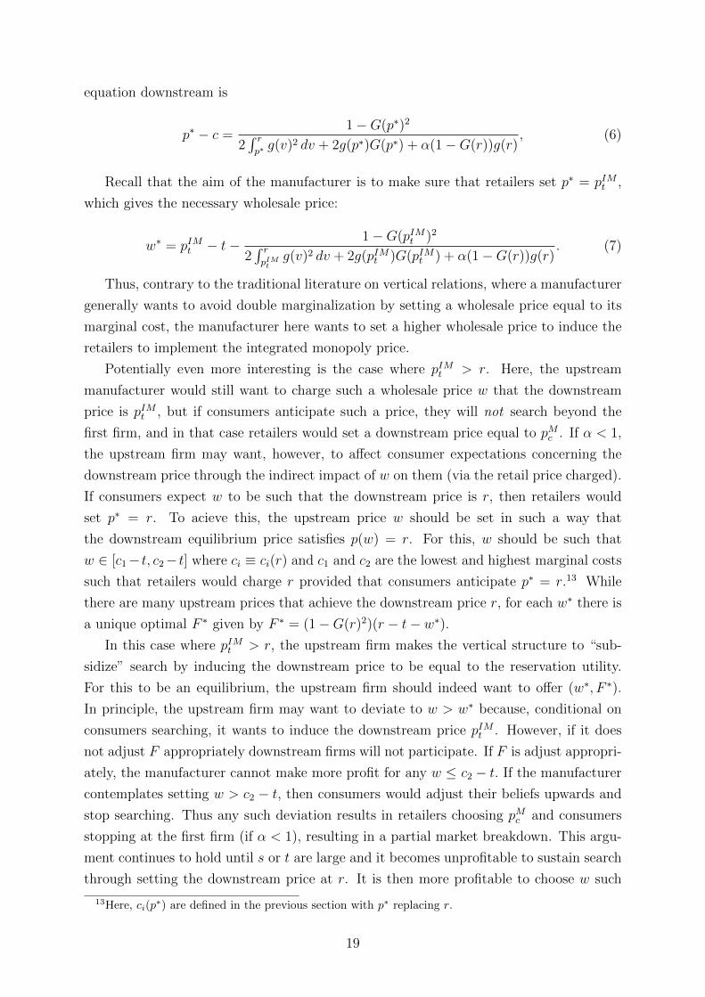
equation downstream is

p∗ − c =1−G(p∗)2

2∫ rp∗g(v)2 dv + 2g(p∗)G(p∗) + α(1−G(r))g(r)

, (6)

Recall that the aim of the manufacturer is to make sure that retailers set p∗ = pIMt ,

which gives the necessary wholesale price:

w∗ = pIMt − t− 1−G(pIMt )2

2∫ rpIMt

g(v)2 dv + 2g(pIMt )G(pIMt ) + α(1−G(r))g(r). (7)

Thus, contrary to the traditional literature on vertical relations, where a manufacturer

generally wants to avoid double marginalization by setting a wholesale price equal to its

marginal cost, the manufacturer here wants to set a higher wholesale price to induce the

retailers to implement the integrated monopoly price.

Potentially even more interesting is the case where pIMt > r. Here, the upstream

manufacturer would still want to charge such a wholesale price w that the downstream

price is pIMt , but if consumers anticipate such a price, they will not search beyond the

first firm, and in that case retailers would set a downstream price equal to pMc . If α < 1,

the upstream firm may want, however, to affect consumer expectations concerning the

downstream price through the indirect impact of w on them (via the retail price charged).

If consumers expect w to be such that the downstream price is r, then retailers would

set p∗ = r. To acieve this, the upstream price w should be set in such a way that

the downstream equilibrium price satisfies p(w) = r. For this, w should be such that

w ∈ [c1− t, c2− t] where ci ≡ ci(r) and c1 and c2 are the lowest and highest marginal costs

such that retailers would charge r provided that consumers anticipate p∗ = r.13 While

there are many upstream prices that achieve the downstream price r, for each w∗ there is

a unique optimal F ∗ given by F ∗ = (1−G(r)2)(r − t− w∗).In this case where pIMt > r, the upstream firm makes the vertical structure to “sub-

sidize” search by inducing the downstream price to be equal to the reservation utility.

For this to be an equilibrium, the upstream firm should indeed want to offer (w∗, F ∗).

In principle, the upstream firm may want to deviate to w > w∗ because, conditional on

consumers searching, it wants to induce the downstream price pIMt . However, if it does

not adjust F appropriately downstream firms will not participate. If F is adjust appropri-

ately, the manufacturer cannot make more profit for any w ≤ c2 − t. If the manufacturer

contemplates setting w > c2 − t, then consumers would adjust their beliefs upwards and

stop searching. Thus any such deviation results in retailers choosing pMc and consumers

stopping at the first firm (if α < 1), resulting in a partial market breakdown. This argu-

ment continues to hold until s or t are large and it becomes unprofitable to sustain search

through setting the downstream price at r. It is then more profitable to choose w such

13Here, ci(p∗) are defined in the previous section with p∗ replacing r.

19

that the downstream price is pMt > r, and no consumer searches beyond the first firm. By

the definition of pMt , the upstream price that induces it is w∗ = 0.

Given the discussion above, we can characterize the pricing decision of the upstream

manufacturer. For α < 1 we do this in a proposition characterizing the equilibrium in

terms of t, while a corollary restates the result in terms of s. We then show (only for

the characterization in terms of t) that the result is very different for α = 1. Finally, we

analyze cost pass-through in the vertical industry structure.

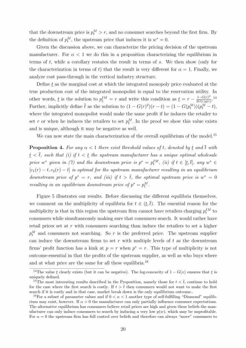
Define t as the marginal cost at which the integrated monopoly price evaluated at the

true production cost of the integrated monopolist is equal to the reservation utility. In

other words, t is the solution to pIMt = r and write this condition as t = r − 1−G(r)2

2G(r)g(r).14

Further, implicitly define t as the solution to (1− G(r)2)(r − t) = (1− G(pMt ))(pMt − t),where the integrated monopolist would make the same profit if he induces the retailer to

set r or when he induces the retailers to set pMt. In the proof we show this value exists

and is unique, although it may be negative as well.

We can now state the main characterization of the overall equilibrium of the model.15

Proposition 4. For any α < 1 there exist threshold values of t, denoted by t and t with

t < t, such that (i) if t < t the upstream manufacturer has a unique optimal wholesale

price w∗ given in (7) and the downstream price is p∗ = pIMt , (ii) if t ∈ [t, t], any w∗ ∈[c1(r)− t, c2(r)− t] is optimal for the upstream manufacturer resulting in an equilibrium

downstream price of p∗ = r, and (iii) if t > t, the optimal upstream price is w∗ = 0

resulting in an equilibrium downstream price of p∗ = pMt .

Figure 5 illustrates our results. Before discussing the different equilibria themselves,

we comment on the multiplicity of equilibria for t ∈ (t, t). The essential reason for the

multiplicity is that in this region the upstream firm cannot have retailers charging pIMt to

consumers while simultaneously making sure that consumers search. It would rather have

retail prices set at r with consumers searching than induce the retailers to set a higher

pMt and consumers not searching. So r is the preferred price. The upstream supplier

can induce the downstream firms to set r with multiple levels of t as the downstream

firms’ profit function has a kink at p = r when p∗ = r. This type of multiplicity is not

outcome-essential in that the profits of the upstream supplier, as well as who buys where

and at what price are the same for all these equilibria.16

14The value t clearly exists (but it can be negative). The log-concavity of 1 − G(x) ensures that t isuniquely defined.

15The most interesting results described in the Proposition, namely those for t < t, continue to holdfor the case where the first search is costly. If t > t then consumers would not want to make the firstsearch if it is costly and in that case, market break down is the only equilibrium outcome..

16For a subset of parameter values and if 0 < α < 1 another type of self-fulfilling “Diamond” equilib-rium may exist, however. If α > 0 the manufacturer can only partially influence consumer expectations.The alternative equilibrium has consumers believe retail prices are high and given these beliefs the man-ufacturer can only induce consumers to search by inducing a very low p(w), which may be unprofitable.For α = 0 the upstream firm has full control over beliefs and therefore can always “move” consumers to

20

��

-��

��

��

��

�

��

-��

��

��

��

�

r

tt1 t2

pMt

pIMt

p⇤

��

��

-��

��

��

��

�

p*

w*

c*c⇤w⇤

r

t

pMt

pIMt

p⇤

��

��

-��

��

��

��

�

p*

w*

c*c⇤w⇤

tt

Figure 5: Downstream and upstream prices as the function of t for G ∼ U(0, 1), s = 0.05,and α = 0. Shaded areas correspond to upstream price multiplicity.

In the range of t where the multiplicity is present, there always are equilibria where

w∗ < 0. The reason should be clear: in this range the upstream firm has to subsidize

search via very low unit price inducing downstream firms to charge r and consumers to

search the second time.

The upstream supplier does not directly control retail prices, however. Conditional

on consumers searching, the supplier has an incentive to increase the retail price to pIM .

However, any deviation to w > c2(r)− t triggers a change in pei used by consumers. The

result is that pe1 = pe2 > r and consumers who draw vi below r at the first firm expect

negative utility from continuing to search and they stop searching. It is clear that α < 1

is essential to this: for passive beliefs (α = 1) the supplier’s temptation to deviate once

consumers have made up their mind about searching (via p∗ ≤ r) is not restrained by

anything, and therefore unavoidable. We will elaborate on the case where α = 1 below.

Note also how at t = t , the optimal upstream supplier’s price w∗ equals 0, which is

when downstream firms are able to charge the integrated monopoly price on their own.

They are effectively able to “collude” aided by beliefs that discourage downward price

deviations. This is true because α = 0 so a unit reduction in price induces consumers to

believe that the firm they have not yet visited had also reduced its price by one unit. Such

a highly collusive price is not feasible for any α > 0 because only a perfect combination of

price-increase friendly beliefs and sufficiently high marginal cost allows retailers to charge

the integrated monopoly price. When t = t , by the definition of t , p∗ = r therefore all

the consumers who search are those who would not buy the good from the first firm they

have visited. This means that firms are setting p1 and p2 knowing that the only consumers

the equilibrium where p∗ = r. As beliefs become less responsive, the range where there is co-existenceof Diamond equilibria without second search and equilibria were the downstream price equals r grows.We do not focus on these equilibria as it is clear that these are not optimal from the monopoly manu-facturer’s point of view. Moreover, the range of parameter values for which these equilibria exist is noteasily characterized.

21

they are losing to the other firm are those who wouldn’t buy from them anyway. This

leads to the firms charging the integrated monopoly price. As the next figure illustrates

in the context of the comparative statics with respect to the search cost s, for α = 0.5 the

downstream firms are not able to charge pIMt without the help of the upstream supplier.

The supplier induces downstream firms to charge pIMt by setting w∗ > 0.

We now restate this result in terms of search cost s. The key finding is that, because r

is inversely related to s, there may be a range of search costs where the equilibrium down-

stream price is decreasing in the search cost. Although we have found a similar pattern in

our earlier paper on vertical relations in a search market with homogeneous goods (Janssen

and Shelegia (2015)), the reason for this result is very different. In Janssen and Shelegia

(2015) the mechanism is as follows: when consumers search for the lowest downstream

price without knowing the upstream price, they have to blame downstream firms for price

deviations above the reservation price, or else equilibrium would break down.17 This then

makes the upstream firm wants to secretly deviate and eat up downstream margins. This

incentive to secretly squeeze retailers results in excessively high equilibrium prices. The

effect is mitigated when downstream firms have more market power and higher margins,

i.e., when search costs are higher, so overall an increase in search costs may result in a

downstream price reduction. In the current model, beliefs are key, and downstream price

is decreasing in the search cost because when α < 1 the upstream firm is able to subsidize

search via low upstream price (inducing retailers to follow suit choosing low downstream

prices).

To state our next result more formally, implicitly define s and s in a similar way to

t and t, i.e., s is the search cost at which the integrated monopoly price evaluated at

the true production cost of the integrated monopolist is equal to the reservation utility.

Furthermore, implicitly define s to be the solution where the integrated monopolist would

make the same profit if it induces the retailers to set r compared to when it induces them

to set pMt .18

Corollary 5. For any α < 1 there exist threshold values of s, denoted by s and s,

with s < s, such that (i) if s < s, the upstream manufacturer has a unique optimal

wholesale price w∗ that is such that the downstream price is p∗ = pIMt , (ii) if s ∈ [s, s],

any w∗ ∈ [c1−t, c2−t] is optimal for the upstream manufacturer resulting in an equilibrium

downstream price of r, and (iii) if s > s, the optimal upstream price is w∗ = 0 resulting

in an equilibrium downstream price of pMt .

The proposition is illustrated in Figure 6 for G ∼ U(0, 1), α = 0.5 and t = 0.1 where

for preservation of space we depict c∗ = w∗ + t instead of w∗. For low search costs the

17If consumers were to accept such prices, then downstream firms would indeed deviate and chargeprices above the reservation price.

18Similar to the previous Proposition, results for s < s continue to hold for the case where the firstsearch is costly.

22

��

-��

��

��

ss3 s4

rpM

tpIM

t

p⇤

c⇤

r

Figure 6: Downstream and upstream prices as the function of s for G ∼ U(0, 1), t = 0.1,and α = 0.5. Shaded areas correspond to upstream price multiplicity.

downstream price is constant, while the wholesale price is decreasing in s. This is because

as s increases, downstream margins grow and therefore the manufacturer does not need to

push the downstream price as much up as it does for lower values of s. In the intermediate

region of search costs the downstream price is equal to r and therefore decreasing in s.

To keep the downstream price at r, the manufacturer has to charge lower and lower

wholesale prices, which may even become negative. For each s in this region there are

multiple values of the equilibrium w∗ because the downstream price as a function of c is

flat (as per Proposition 3). If s is sufficiently high, the upstream firm no longer subsidizes

search, and induces a single-good monopoly price that is above r. That is, even though

the manufacturer is still able to prevent partial market breakdown, it is not in his interest

to do so as he has to distort the retail price too much to make it possible.

It is interesting to observe that the two-part tariff we imposed is actually also the

optimal contract in the general class of non-linear contracts. Industry profits are highest

if retailers price at the integrated profit maximizing pIMt . With the nonlinear contract we

specified, for s < s1(r) the manufacturer will set its wholesale price per unit w such that

retailers find it optimal to choose r and extract all retailers’ profit by choosing the fixed

fee appropriately. For larger s, the manufacturer is constrained by retail and consumer

behavior, but sets w such that retail prices are as close as possible to pIMt given these

constraints.

Finally, we should note that the manufacturer does not have any incentive to foreclose

one of the retailers by setting a contract the retailer will not accept. The main reason is

that the manufacturer benefits from the diversity that is offered by the retailers, where

different consumers prefer buying from different retailers creating more demand for the

manufacturer than would be the case with only one retailer. Interestingly, a similar

argument holds true for the question whether the manufacturer wants to sell through

retailers at all, or prefers to sell directly. As long as retailers can create diversity that

is difficult to replicate by one single manufacturer, where this diversity is important to

23

attract different types of consumers that would otherwise not buy or not continue to

search, the manufacturer benefits by selling through retailers.

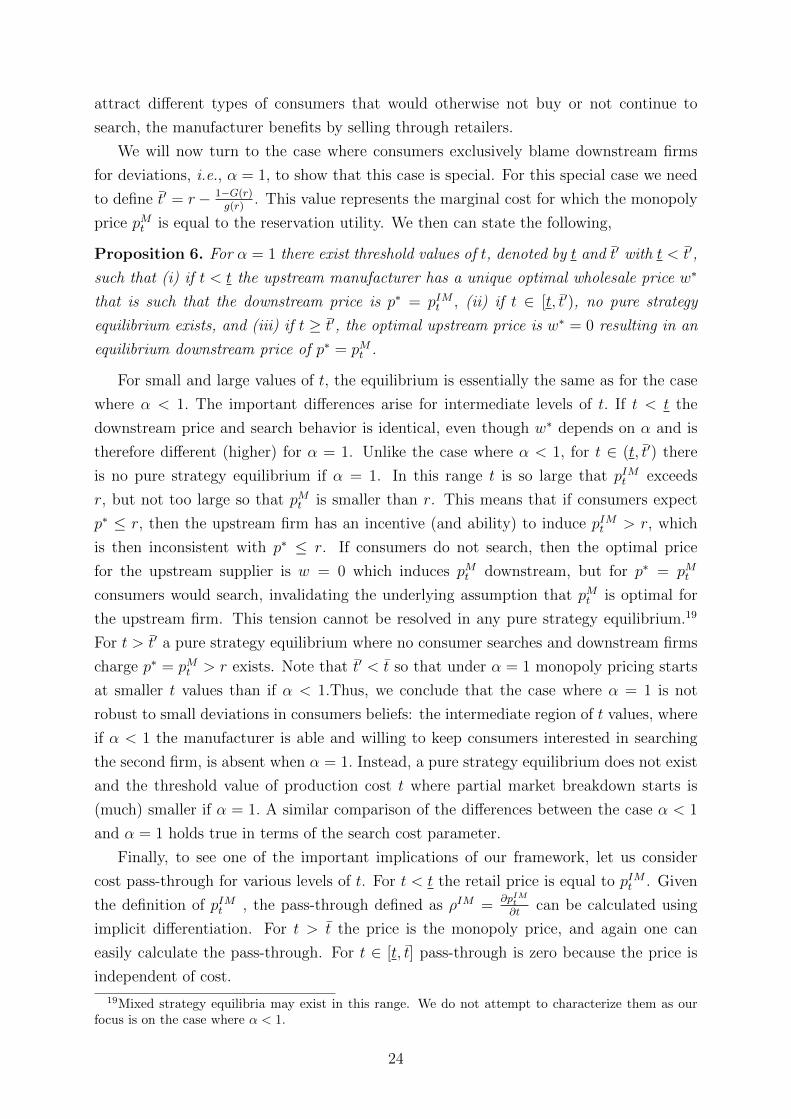
We will now turn to the case where consumers exclusively blame downstream firms

for deviations, i.e., α = 1, to show that this case is special. For this special case we need

to define t′ = r− 1−G(r)g(r)

. This value represents the marginal cost for which the monopoly

price pMt is equal to the reservation utility. We then can state the following,

Proposition 6. For α = 1 there exist threshold values of t, denoted by t and t′ with t < t′,

such that (i) if t < t the upstream manufacturer has a unique optimal wholesale price w∗

that is such that the downstream price is p∗ = pIMt , (ii) if t ∈ [t, t′), no pure strategy

equilibrium exists, and (iii) if t ≥ t′, the optimal upstream price is w∗ = 0 resulting in an

equilibrium downstream price of p∗ = pMt .

For small and large values of t, the equilibrium is essentially the same as for the case

where α < 1. The important differences arise for intermediate levels of t. If t < t the

downstream price and search behavior is identical, even though w∗ depends on α and is

therefore different (higher) for α = 1. Unlike the case where α < 1, for t ∈ (t, t′) there

is no pure strategy equilibrium if α = 1. In this range t is so large that pIMt exceeds

r, but not too large so that pMt is smaller than r. This means that if consumers expect

p∗ ≤ r, then the upstream firm has an incentive (and ability) to induce pIMt > r, which

is then inconsistent with p∗ ≤ r. If consumers do not search, then the optimal price

for the upstream supplier is w = 0 which induces pMt downstream, but for p∗ = pMt

consumers would search, invalidating the underlying assumption that pMt is optimal for

the upstream firm. This tension cannot be resolved in any pure strategy equilibrium.19

For t > t′ a pure strategy equilibrium where no consumer searches and downstream firms

charge p∗ = pMt > r exists. Note that t′ < t so that under α = 1 monopoly pricing starts

at smaller t values than if α < 1.Thus, we conclude that the case where α = 1 is not

robust to small deviations in consumers beliefs: the intermediate region of t values, where

if α < 1 the manufacturer is able and willing to keep consumers interested in searching

the second firm, is absent when α = 1. Instead, a pure strategy equilibrium does not exist

and the threshold value of production cost t where partial market breakdown starts is

(much) smaller if α = 1. A similar comparison of the differences between the case α < 1

and α = 1 holds true in terms of the search cost parameter.

Finally, to see one of the important implications of our framework, let us consider

cost pass-through for various levels of t. For t < t the retail price is equal to pIMt . Given

the definition of pIMt , the pass-through defined as ρIM =∂pIMt∂t

can be calculated using

implicit differentiation. For t > t the price is the monopoly price, and again one can

easily calculate the pass-through. For t ∈ [t, t] pass-through is zero because the price is

independent of cost.

19Mixed strategy equilibria may exist in this range. We do not attempt to characterize them as ourfocus is on the case where α < 1.

24

� ��

��

��

��

t1 t2

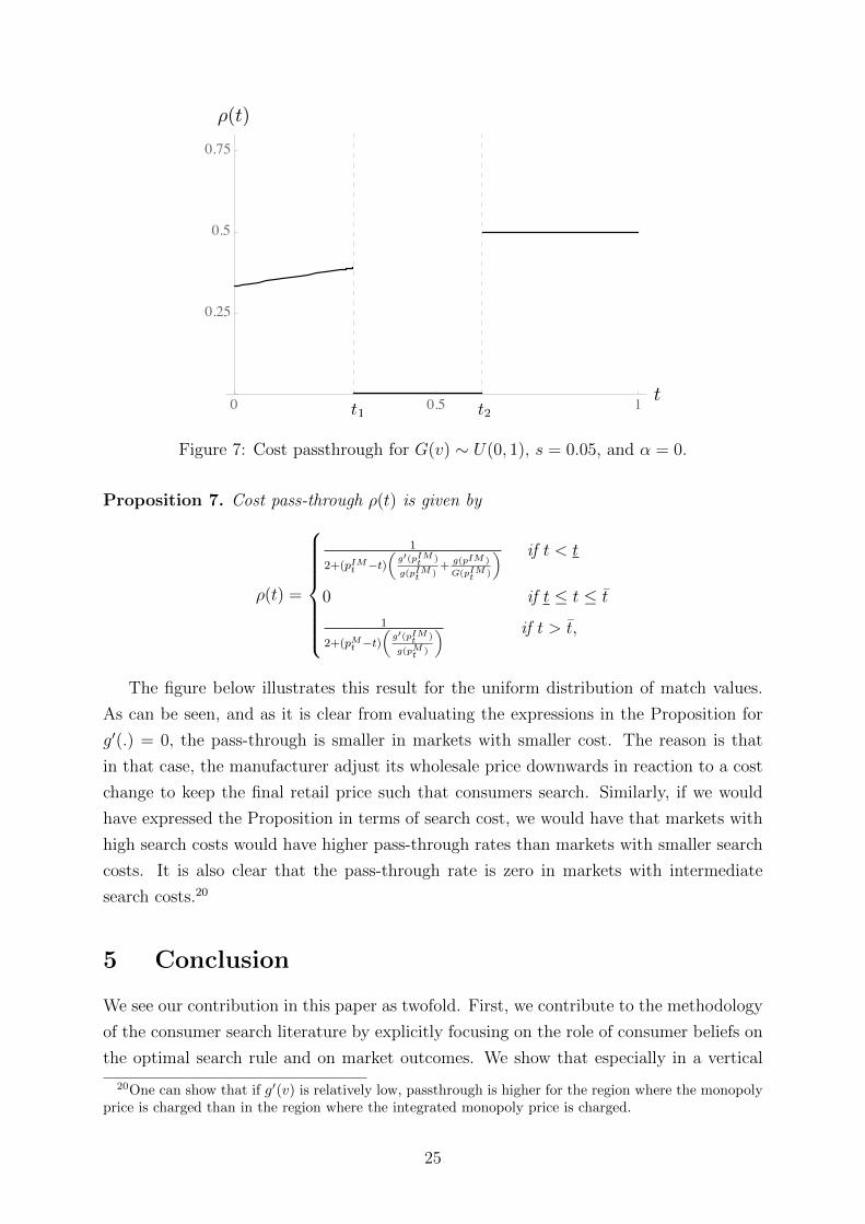
⇢(t)

t

Figure 7: Cost passthrough for G(v) ∼ U(0, 1), s = 0.05, and α = 0.

Proposition 7. Cost pass-through ρ(t) is given by

ρ(t) =

1

2+(pIMt −t)(

g′(pIMt )

g(pIMt )+

g(pIM )

G(pIMt )

) if t < t

0 if t ≤ t ≤ t

1

2+(pMt −t)(

g′(pIMt )

g(pMt )

) if t > t,

The figure below illustrates this result for the uniform distribution of match values.

As can be seen, and as it is clear from evaluating the expressions in the Proposition for

g′(.) = 0, the pass-through is smaller in markets with smaller cost. The reason is that

in that case, the manufacturer adjust its wholesale price downwards in reaction to a cost

change to keep the final retail price such that consumers search. Similarly, if we would

have expressed the Proposition in terms of search cost, we would have that markets with

high search costs would have higher pass-through rates than markets with smaller search

costs. It is also clear that the pass-through rate is zero in markets with intermediate

search costs.20

5 Conclusion

We see our contribution in this paper as twofold. First, we contribute to the methodology

of the consumer search literature by explicitly focusing on the role of consumer beliefs on

the optimal search rule and on market outcomes. We show that especially in a vertical

20One can show that if g′(v) is relatively low, passthrough is higher for the region where the monopolyprice is charged than in the region where the integrated monopoly price is charged.

25

market, this role is important. In particular, the standard assumption in the consumer

search literature following Wolinsky (1986) is that, upon any observed price deviation,

consumers believe that non-observed prices are equal to their equilibrium values. In the

terminology of the vertical relations literature: consumers exclusively blame individual

retailers they visited for observing an unexpected price. We show that the equilibrium

predictions using this assumption are not robust to slight changes in beliefs: assuming that

consumers attach a non-zero probability to the possibility that the upstream supplier’s

deviation is the cause of the unexpected retail price leads to qualitatively different results.

Second, using robust beliefs, we provide a number of new explanations for a range

of different observations. For example, we show why the downstream (and wholesale)

market price can be non-monotonic in search cost and independent of the marginal cost

for a range of parameter values. We also show that retailers may price at the joint profit

maximizing price even if they choose their pricing strategies in a noncooperative way.

Finally, we show how our model with homogeneous search costs generates price rigidities

in a natural way as firms have an incentive to charge prices so that consumers do not

continue to search the next firm. This phenomenon occurs as the manufacturer has an

incentive and the ability to pro-actively prevent a partial market breakdown by lowering

its price. It is not difficult to see that for a small search cost heterogeneity (see, also,

Moraga-Gonzalez, Sandor and Wildenbeest (2014)) retail prices will not react much to

changes in marginal cost. Many industries are characterized by incomplete cost pass-

through (Weyl and Fabinger (2013)), i.e., higher wholesale prices induce lower margins

at the retail level. In our model, low levels of cost pass-through arise because of retailers,

but especially manufacturers, optimally reacting to consumer search.

Our model is purposefully simple in nature. We did not study retail oligopoly, or

wholesale competition, or other arrangements (such as exclusive dealing) that are typically

found in wholesale markets. We see our paper as building the foundations for a literature

studying the implications of consumer search in a vertical supply channel. We have shown

the basic issues to be addressed to understand pricing in the vertical channel. We have

shown that these issues are nontrivial, and fundamentally different from when consumers

have full information (as is typically the case in the vertical relations literature). In

subsequent research other non-price issues that are important in the vertical relations

literature can be added to the model we have outlined.

References

Akerlof, George A., and Janet L. Yellen. 1985a. “Can Small Deviations from Ra-

tionality Make Significant Differences to Economic Equilibria?” American Economic

Review, 75(4): 708–720.

26

Akerlof, George A., and Janet L. Yellen. 1985b. “A Near-rational Model of the

Business Cycle, with Wage and Price Intertia.” The Quarterly Journal of Economics,

100(5): 823–838.

Anderson, Simon P., and Regis Renault. 1999. “Pricing, Product Diversity, and

Search Costs: A Bertrand-Chamberlin-Diamond Model.” RAND Journal of Economics,

30(4): 719–735.

Anderson, Simon P., and Regis Renault. 2006. “Advertising Content.” American

Economic Review, 96(1): 93–113.

Armstrong, Mark, and Jidong Zhou. 2015. “Search deterrence.” The Review of Eco-

nomic Studies, 83(1): 26–57.

Armstrong, Mark, John Vickers, and Jidong Zhou. 2009. “Prominence and Con-

sumer Search.” The RAND Journal of Economics, 40(2): 209–233.

Asker, John, and Heski Bar-Isaac. 2017. “Vertical Information Restraints: Pro- and

Anti-Competitive Impacts of Minimum Advertised Price Restrictions.” Mimeo.

Bar-Isaac, Heski, Guillermo Caruana, and Vicente Cunat. 2011. “Search, Design

and Market Structure.” American Economic Review, 102(2): 1140–60.

Cabral, Luıs, and Arthur Fishman. 2012. “Business as Usual: A Consumer Search

Theory of Sticky Prices and Asymmetric Price Adjustment.” International Journal of

Industrial Organization, 30(4): 371–376.

Diamond, Peter A. 1971. “A Model of Price Adjustment.” Journal of Economic Theory,

3(2): 156–168.

Garcia, Daniel, Maarten C.W. Janssen, and Jun Honda. 2017. “The Double

Diamond Paradox.” AEJ Microeconomics, 9(3): 63–99.

Hart, Oliver, Jean Tirole, Dennis W. Carlton, and Oliver E. Williamson. 1990.

“Vertical integration and Market Foreclosure.” Brookings Papers on Economic Activity.

Microeconomics, 205–286.

Janssen, Maarten C.W., and Sandro Shelegia. 2015. “Consumer Search and Double

Marginalization.” American Economic Review, 105(6): 1683–1710.

Janssen, Maarten C.W., Jose Luis Moraga-Gonzalez, and Matthijs R. Wilden-

beest. 2005. “Truly Costly Sequential Search and Oligopolistic Pricing.” International

Journal of Industrial Organization, 23(5-6): 451–466.

27

Karle, Heiko, Martin Peitz, and Markus Reisinger. 2017. “Segmentation versus

Agglomeration: Competition between Platforms with Competitive Sellers.” Mimeo.

Lubensky, Dmitry. 2017. “A model of recommended retail prices.” The RAND Journal

of Economics, 48(2): 358–386.

Mankiw, N. Gregory. 1985. “Small Menu Costs and Large Business Cycles: A Macroe-

conomic Model of Monopoly.” The Quarterly Journal of Economics, 100(2): 529–538.

McAfee, R. Preston, and Marius Schwartz. 1994. “Opportunism in Multilateral

Vertical Contracting: Nondiscrimination, Exclusivity, and Uniformity.” American Eco-

nomic Review, 84(1): 210–30.

Moraga-Gonzalez, Jose Luis, Zsolt Sandor, and Matthijs R. Wildenbeest. 2014.

“Prices, Product Differentiation, And Heterogeneous Search Costs.”

Moraga-Gonzalez, Jose Luis, Zsolt Sandor, and Matthijs R Wildenbeest.

2017. “Prices and Heterogeneous Search Costs.” The RAND Journal of Economics,

48(1): 125–146.

Sherman, Joshua, and Avi Weiss. 2015. “Price Response, Asymmetric Information

and Competition.” The Economic Journal, 125(589): 2077–2115.

Sheshinski, Eytan, and Yoram Weiss. 1977. “Inflation and Costs of Price Adjust-

ment.” Review of Economic Studies, 44(2): 287–303.

Stahl, Dale O. 1989. “Oligopolistic Pricing with Sequential Consumer Search.” Ameri-

can Economic Review, 79(4): 700–712.

Wang, Chengsi, and Julian Wright. 2017. “Search Platforms: Showrooming and

Price Parity Clauses.” Mimeo.

Weyl, E Glen, and Michal Fabinger. 2013. “Pass-through as an Economic Tool:

Principles of Incidence Under Imperfect Competition.” Journal of Political Economy,

121(3): 528–583.

Wolinsky, Asher. 1986. “True Monopolistic Competition as a Result of Imperfect In-

formation.” Quarterly Journal of Economics, 101(3): 493–511.

Zhou, Jidong. 2014. “Multiproduct search and the joint search effect.” The American

Economic Review, 104(9): 2918–2939.

28

Appendix: Proofs

Proposition 1. If the utility distribution G(v) is uniformly distributed on [0, 1], then a

symmetric downstream equilibrium exists and is unique.

Proof. Consider the match function to be the uniform distribution over [0, 1]. We first

prove the strict concavity of the profit function when pi < p. We distinguish two cases:

(i) pj p.

In the first case the demand qi(pi, pj, p∗) of firm i observing w 6= w∗ and setting price

pi believes the other firm sets pj = p(w) while the ex ante consumer expectation of prices

is p∗, is given by the four components in Figure 1 where we set pej = αp∗ + (1− α)pi and

pei = αp∗ + (1 − α)pj. Thus, (assuming the regions are not empty) the size of the four

regions being A,B,C and D is equal to, respectively

1− r + α(p∗ − pi)

(r − αp∗ − (1− α)pi)

(pj +

1

2(r − αp∗ − (1− α)pi)

)[1− r − pi + αp∗ + (1− α)pj)] (r − α(p∗ − pj))

[r − αp∗ − (1− α)pj)]

(pj +

1

2(r − α(p∗ − pj)− pj)

).

Thus, the profit function πi = qi(pi, pj, p∗)(pi−c) is concave if ∂2πi/∂p

2i = 2∂qi(pi, pj, p

∗)/∂pi+

(pi− c)∂q2i (pi, pj, p

∗)/∂p2i < 0, where we have to take into account that ∂pej/∂pi = (1−α)

as pej = αp∗ + (1− α)pi. As

∂qi(pi, pj, p∗)

∂pi= −α− (1− α) (pj + r − αp∗ − (1− α)pi)− (r − α(p∗ − pj))

= −α + (1− α)2pi − (2− α)(r − αp∗)− pj

and∂q2

i (pi, pej , p∗)

∂p2i

= (1− α)2.

Thus,

∂2πi/∂p2i = 2

[−α + (1− α)2pi − (2− α)(r − αp∗)− pj

]+ (1− α)2(pi − c).

As pi − c < pi < p = r−αp∗1−α it is clear that this expression is smaller than

2 [−α + (1− α)(r − αp∗)− (2− α)(r − αp∗)− pj] + (1− α)(r − αp∗)= −2 [α + (r − αp∗) + pj] + (1− α)(r − αp∗) < 0

Hence, the profit function is strictly concave for pi p. in this case, firm i does not attract any consumer

29

who first visited firm j as these consumers believe that firm i sets such a high price that

it is not worthwhile to incur the search cost s. Thus, only regions A and B are relevant

for consumer demand. In this case, using pi − c < pi p we have

∂2πi/∂p2i = 2 [−α− (1− α)(r − αp∗ − (1− α)pi)− (1− α)pj] + (1− α)2(pi − c)< 2 [−α− (1− α)pj] + (1− α)(r − αp∗)< −2α− (1− α)pj − α(r − αp∗) < 0.

Thus, we have now proved that the profit function is strictly concave for pi < p.

Next consider prices such that pi > p. In this case as p = r−αp∗1−α we have that pi >

r−α(p∗−pi) such that region B is empty: firm i does not get any returning consumers as

no consumer who first visited firm i continues to search firm j in the first place. Again,

we have to distinguish two cases: (i) pj p.

If pj < p, then firm i receives demand from regions A,C and D. Thus,

∂qi(pi, pj, p∗)

∂pi= −α− (r − α(p∗ − pj))

and

∂2πi/∂p2i = 2 [−α− (r − αp∗)− αpj] + (1− α)2(pi − c).

This expression is clearly increasing in pi, while it is negative at pi = p. Thus, either

∂2πi/∂p2i < 0 for all values of pi or there is a cut-off value for pi such that for larger values

∂2πi/∂p2i > 0, while for smaller values it is negative. In the former case the profit function

is strictly concave, while in the latter case it is strictly quasi-concave due to the fact that

qi(1, pj, p∗) = 0, while qi(pi, pj, p

∗) > 0 for all pi < 1.

If pj > p, then firm i effectively also does not get any demand from consumers who

first visited firm j. Demand is therefore (1 − G(pi)) = 1 − pi and it is clear the profit

function is strictly concave.

Finally, we need to establish that for any given pj the overall profit function is (at

least) strictly quasi-concave. We show that for each pj the left-hand side derivative

of the profit function at pi = p is larger than or equal to the right-hand side deriva-

tive of the profit function, i.e., limpi↑p ∂πi/∂pi > limpi↓p ∂πi/∂pi. Together with the

strict concavity of the profit function for pi p (and limpi↓p ∂2πi/∂p

2i < 0 if pj < p) this establishes the overall strict quasi-

concavity of the profit function. Consider pj ≤ p first. We have seen above that the

demand for firm i comprises the areas C and D, independent of whether or not pI < p.

Thus, if there is a difference in the left- and right-hand derivatives it should be rela-

tive to the demand regions A and B. Similarly, if we consider pj > p, then anyway

only the demand regions A and B are relevant as no consumer that first visited firm

30

j would visit firm i. Thus, independent of whether or not pj ≤ p we only need to

establish that limpi↑p ∂qi(pi, pj, p∗)/∂pi ≥ limpi↓p ∂qi(pi, pj, p

∗)/∂pti as ∂πi/∂pi = (pi −c)∂qi(pi, pj, p

∗)/∂pi + qi(pi, pj, p∗) and limpi↑p qi(pi, pj, p

∗) = limpi↓p qi(pi, pj, p∗). It is clear

that limpi↑p ∂qi(pi, pj, p∗)/∂pi = −G(r + pj − αp∗ − (1 − α)pi) − αg(r − α(p∗ − pi))(1 −

G(r + pj − αp∗ − (1 − α)pi)) ≥ −1, whereas limpi↓p ∂qi(pi, pj, p∗)/∂pi = −1. Thus, for

any utility distribution function G(.) the left-hand side derivative of the profit function

at pi = p is larger than or equal to the right-hand side derivative of the profit function.

If the inequality is strict, there is a kink in the profit function.

As the profit function is strictly quasi-concave in pi the best response function pi(pj; p∗, c)

is well defined for each value of consumer expectation p∗ and each value of the firm’s cost

c. As the profit function πi = qi(pi, pj, p∗)(pi − c) is continuous in pi and pj the best re-

sponse functions are also continuous and a standard fixed point argument then establishes

the existence of a symmetric equilibrium.

Uniqueness of a symmetric equilibrium follows from the following considerations. First,

within the two regions pi = pj p an equilibrium is unique if the slope

of the best response function

dpidpj

= −∂2πi/∂pi∂pj∂2πi/∂p2

i

< 1.

In the region pi = pj < p,

∂2qi/∂pj = (1− α)(r − α(p∗ − pj)) + α [1− r − pi + αp∗ + (1− α)pj)]

−1

2(1− α) (pj + (r − α(p∗ − pj))) +

1

2(1− α) [r − αp∗ − (1− α)pj)]

= (1− α)2(p− pj) + α(1− pi).

Thus, as ∂2πi/∂pi∂pj = ∂qi(pi, pj, p∗)/∂pj + (pi − c)∂q2

i (pi, pj, p∗)/∂pi∂pj,

dpidpj

< 1 if , and

only if,

(1− α)2(p− pj) + α(1− pi)− (pi − c)< 2

[α− (1− α)2pi + (2− α)(r − αp∗) + pj

]− (1− α)2(pi − c)

As in a symmetric equilibrium pi = pj this reduces to

(p− pi) + α(1− pi) < α(2− α)(pi − c) + 2α + 2(2− α)p,

which is always the case.

Clearly, as in the region pi = pj > p, ∂2πi/∂pi∂pj = 0 and there is a unique monopoly

price, there can only be a unique equilibrium in this region.

Proposition 2. For given parameter values s and α and a given consumer belief about

31

the downstream price p∗ the symmetric downstream equilibrium price p(w) is given by

p(w) =

p if c ≤ c1(p∗)

p if c1(p∗) < c ≤ c2(p∗)

pMc if c > c2(p∗),

where p solves (3). In this equilibrium consumers search for c ≤ c2(p∗) and do not search

otherwise.

Proof. Let us start with c > c2(p∗). We first establish that p = pMc is indeed an equi-

librium. If firm j charges pj = pMc then firm i does not receive any second visits from j

because by definition of c2(p∗) we have pMc > p and therefore consumers arriving to j set

pei > r and do not search. Given that no second visits occur, firm i cannot do better than

to charge the monopoly price, and sell to all consumers who arrive to it. In this case,

consumers who make first visits to i will not search either, giving i (maximum possible)

monopoly profits. Having verified that pi = pj = pMc is an equilibrium, we now show that

no other equilibrium exists. Assume the equilibrium price p satisfies p > p but p 6= pMc .

This cannot be an equilibrium because no consumers search, and therefore each firm is

better off charging the monopoly price pMc . Assume now that p ≤ p. In such equilibrium

consumers would search. Conditional on consumers searching (Ir≥pei = 1) the symmetric

equilibrium price has to satisfy (3). Moving the RHS to the left and taking derivative with

respect to p reveals that the derivative is positive by log-concavity of 1−G(x). Plugging

p instead of p yields p− 1−G(p)2

(α+(2−α)G(p))g(p)− c, which is negative by c > c2(p∗) ≥ c1(p∗) and

the definition of c1(p∗). It is therefore impossible that p that solves (3) simultaneously

satisfies p < p.

Assume now that c < c1(p∗). Given that consumers search, the symmetric equilibrium

price has to be p. For this to be true, we need that p ≤ p. This follows using similar

steps as above. If consumers do not search, then both firms aught to charge pMc , but c <

c1(p∗) ≤ c2(p∗) and therefore pMc < p so consumers would search in such an equilibrium,

a contradiction.

Finally, assume c1(p∗) < c ≤ c2(p∗). First let us prove that p = p is indeed an

equilibrium. Assume firm j charges pj = p. Then for firm i demand is given by

qi(pi, pj, p∗) = (1−G(pi + max{r − pej , 0})) +

∫ pi+max{r−pej ,0}

pi


+G(pj)(1−G(pi))

Assume that pi ≤ p so that consumers who visit i first and draw low utility go on to

search j, and then evaluate the derivative of profit of i at pi = p, to get ∂πi∂pi

(pi = p) =

32

(p − c)g(p)((1 − a)G(p) + a + G(r)) + (1 − G(p))(1 + G(r)) > 0, which by concavity of

profits to the left of p means that the maximizer cannot be pi < p. Now assume pi > p.

In this region the profit is proportional to the monopoly one, and is therefore maximized

at pMc . By the definition of c2(p∗), pMc < p, therefore the profit is decreasing for all p > p

and is again maximized at p. That no equilibrium with p c1(p∗) and similar steps as above. For p > p there would be no search, so both firms

would optimally charge pMc which by c < c2(p∗) contradicts p > p.

Corollary 3. For given parameter values c and α and a given consumer belief about

the downstream price p∗, there exist s1(p∗) and s2(p∗) defined above, with s1(p∗) ≤ s2(p∗),

such that

p =

p if s ≤ s1(p∗)

p if s1(p∗) < s ≤ s2(p∗)

pMc if s > s2(p∗),

Proof. Proof follows essentially the same steps as the proof of Proposition 3. This is

because r is strictly decreasing in s which means that p is also strictly decreasing in s. It is

therefore true that s ≤ s1(p∗) iff c < c1(p∗), s1(p∗) < s ≤ s2(p∗) iff c1(p∗) < c ≤ c2(p∗) and

s > s2(p∗) iff c > c2(p∗). Once this is established, the proof of Proposition 3 suffices.

Proposition 4. For any α < 1 there exist threshold values of t, denoted by t and

t with t < t, such that (i) if t < t the upstream manufacturer has a unique optimal

wholesale price w∗ given in (7) and the downstream price is p∗ = pIMt , (ii) if t ∈ [t, t],

any w∗ ∈ [c1(r) − t, c2(r) − t] is optimal for the upstream manufacturer resulting in an

equilibrium downstream price of p∗ = r, and (iii) if t > t, the optimal upstream price is

w∗ = 0 resulting in an equilibrium downstream price of p∗ = pMt .

Proof. Let us first prove that t and t and are uniquely defined. For t existence and

uniqueness is trivial. For t note that (1−G(r)2)(r − t) = (1−G(pMt ))(pMt − t), can only

hold for pMt > r, which then means that where it holds (1−G(r)2) > (1−G(pMt )). The

derivative of the LHS is −(1−G(r)2), and of the RHS is −(1−G(pMt )). Therefore, if the

equation holds for some t, given that (1−G(pMt )) is decreasing in t, for any t′ > t we have

−(1−G(pMt′ )) > −(1−G(r)2) so that for no such t′ will the equality hold. Therefore the

solution is unique. For existence note that at t = r the LHS is zero, whereas the RHS

is strictly positive. For t sufficiently low, the LHS will exceed the RHS. To prove this,

find x such that (1 − G(x)) > (1 − G(r)2), then we can find t sufficiently low so that

(1 − G(x))(x − t) > (1 − G(r)2)(r − t), then for this t by the definition of pMt we have

(1−G(pMt ))(pMt − t) ≥ (1−G(x))(x− t) > (1−G(r)2)(r− t). Therefore the solution has

to exist.

33

For t < t, note that by the definition of t, at t = t the LHS of (1 − G(r)2)(r − t) =

(1−G(pMt ))(pMt − t) has to exceed the RHS. We cannot have t > t because for any t > t

the RHS has to exceed the LHS (see the argument above), which then contradicts the

statement that at t the opposite is true, therefore t < t.

Assume t < t, then pIMt < r by the definition of pIMt and t. First let us prove that

w∗ = pIMt − t− 1−G(pIMt )2

2∫ r

pIMtg(v)2 dv+2g(pIMt )G(pIMt )+α(1−G(r))g(r)

with p(w∗) = p∗ = pIMt is indeed an

equilibrium. For downstream firms pricing was characterized earlier, and indeed for c =

pIMt − 1−G(pIMt )2

2∫ r

pIMtg(v)2 dv+2g(pIMt )G(pIMt )+α(1−G(r))g(r)

they will set p(w∗) = pIMt . The upstream sup-

plier has no profitable deviation because the vertical structure achieves maximum possible

profits with p(w∗) = pIMt . To show that no other equilibria exists, assume that consumers

expect p∗ 6= pIMt . There are two cases. First consider p∗ < pIMt . For this to be equilib-

rium, the upstream supplier has to charge w∗ = p∗− t− 1−G(p∗)2

2∫ rp∗ g(v)2 dv+2g(p∗)G(p∗)+α(1−G(r))g(r)

,

but then a upward deviation in w (with a corresponding increase in F ) would increase

p∗and would thus increase the upstream supplier’s profits. For p∗ > pIMt there are further

two cases, with p∗ ≤ r and p∗ > r. In the first case the upstream supplier can marginally

reduce w and increase total and thus its own profits. In the second case, consumers would

not search if prices were equal to p∗, but then each downstream firm would charge pMc ,

therefore it would be optimal for the upstream supplier to set w∗ = 0, which then means

that p∗ = pMt , which by t < t then contradicts p∗ > r because r is the integrated monopoly

price for t, so pMt has to be lower both because it is a single-product monopoly price and

for a lower marginal cost t.

Now consider t ∈ [t, t]. Here we have to prove that w∗ ∈ [c1−t, c2−t] is an equilibrium.

There may be another equilibrium where consumers do not search, w∗ = 0 and p(w∗) = pMt

for α > 0, but we ignore them here as explained above. Given that t ∈ [t, t], p∗ = r

and downstream pricing behavior, the upstream supplier cannot do better by lowering

w (there is no change in p(w) or there is a reduction, which then reduces total profits).

An increase in w may again have no effect, or lead to an increase of p(w) which the

triggers an increase in pe above r and thus no consumer searches. The best possible profit

of the vertical structure in that case is 2(1 − G(pMt ))(pMt − t), which by t < t is lower

than 2(1 − G(r)2)(r − t), the latter being the equilibrium profit of the upstream firm,

so no deviation is profitable. As for downstream firms, their pricing for p∗ = r given in

Proposition 2 induces them to charge p(w) = p = r for all w∗ ∈ [c1 − t, c2 − t].Finally, when t > t, if the upstream supplier charges w∗ = 0 and p∗ = pMt consumers

would not search because pMt > r by the definition of t as the solution to (1−G(r)2)(r−t) =

(1 − G(pMt ))(pMt − t) which implies that form t = t we should have r < pMt , and so for

t > t this inequality is preserved. Conditional on consumers not searching, and w∗ = 0,

the downstream firms will indeed optimally charge p(w∗) = pMt . The upstream firm

cannot deviate profitably. A deviation to w > 0 is unprofitable because it will increase

already optimal downstream price. A deviation to w < 0 may at best lead to consumers

34

searching, which given that pIMt > r can at most generate 2(1 − G(r)2)(r − t) for the

vertical structure, which by the definition of t is lower than 2(1 − G(pMt ))(pMt − t). No

other equilibrium may exist. For p∗ > r and p∗ 6= pMt , consumers would not search, and

then the upstream firm would induce p(w) = pMt . For p∗ < r, conditional on consumers

searching, the upstream firm would want to increase p(w) to move it closer to pIM , which

is a profitable deviation.

Corollary 5. For any α < 1 there exist threshold values of s, denoted by s and

s, with s < s, such that (i) if s < s, the upstream manufacturer has a unique optimal

wholesale price w∗ that is such that the downstream price is p∗ = pIMt , (ii) if s ∈ [s, s], any

w∗ ∈ [c1 − t, c2 − t] is optimal for the upstream manufacturer resulting in an equilibrium

downstream price of r, and (iii) if s > s, the optimal upstream price is w∗ = 0 resulting

in an equilibrium downstream price of pMt .

Proof. First let us show that s < s. Both exist by pIMt ∈ [v, v] and the definition of r.

The inequality follows from pIMt > pMt and (1−G(x)2)(x− t) > (1−G(x))(x− t).The rest of the proof follows the same lines as the proof of Proposition 4. For this

note that s < s iff t < t, and s < s iff t < t.

Proposition 6. For α = 1 there exist threshold values of t, denoted by t and t′ with

t < t′, such that (i) if t < t the upstream manufacturer has a unique optimal wholesale

price w∗ that is such that the downstream price is p∗ = pIMt , (ii) if t ∈ [t, t′), no pure

strategy equilibrium exists, and (iii) if t ≥ t′, the optimal upstream price is w∗ = 0

resulting in an equilibrium downstream price of p∗ = pMt .

Proof. We first show t′ > t. This follows from respective definitions and the fact that1−G(r)2

2G(r)g(r)− 1−G(r)

g(r)= (1−G(r))2

2G(r)g(r)> 0. For t ≤ t, the proof is very similar to the proof for

α < 1. Namely, the upstream supplier can charge such w that downstream firms charge

p(w) = pIMt , which then achieves maximal profits for the supplier and thus it has no

profitable deviation. For w∗ = pIMt − t − 1−G(pIMt )2

2∫ r

pIMtg(v)2 dv+2g(pIMt )G(pIMt )+(1−G(r))g(r)

, as shown

in the previous section, downstream equilibrium will result in pIMt charged downstream,

and because t ≤ t, pIMt ≤ r, so consumers will search, thus we have an equilibrium. For

t > t′, it is easy to see that w∗ = 0 is optimal for the upstream firm. In this case the only

equilibrium downstream is such that p(w∗) = pMt , and consumers do not search because

by the definition of t′ we have pMt > r. Since beliefs do not change with prices, there can

be no equilibrium where consumers set p∗ < r because then they would search, and so

the upstream supplier would induce p(w) = pIMt > r which then would contradict p∗ < r.

Given that consumers will not search in equilibrium, the upstream firm cannot do better

than w∗ = 0 and extract all downstream profits with F . Finally, for t ∈ (t, t′] we need to

prove that no pure strategy equilibrium exists. Assume to the contrary that there is w∗

35

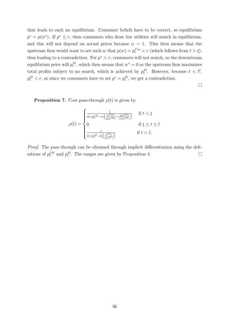
that leads to such an equilibrium. Consumer beliefs have to be correct, so equilibrium

p∗ = p(w∗). If p∗ ≤ r, then consumers who draw low utilities will search in equilibrium,

and this will not depend on actual prices because α = 1. This then means that the

upstream firm would want to set such w that p(w) = pI′mt > r (which follows from t > t),

thus leading to a contradiction. For p∗ > r, consumers will not search, so the downstream

equilibrium price will pMc , which then means that w∗ = 0 so the upstream firm maximizes

total profits subject to no search, which is achieved by pMt . However, because t < t′,

pMt < r, so since we consumers have to set p∗ = pMt , we get a contradiction.

Proposition 7. Cost pass-through ρ(t) is given by

ρ(t) =

1

2+(pIMt −t)(

g′IM )

g(pIM )+

g(pIM )

G(pIM )

) if t < t

0 if t ≤ t ≤ t

1

2+(pMt −t)(

g′M )

g(pM )

) if t > t,

Proof. The pass through can be obtained through implicit differentiation using the defi-

nitions of pIMt and pMt . The ranges are given by Proposition 4.

36

beliefs and consumer search in a vertical industry

Documents