benchmark computations of 3d laminar flow around a ... · benchmark computations of 3d laminar flow...

Benchmark Computations of 3D Laminar FlowAround a Cylinder with CFX, OpenFOAM and FeatFlow

E. Bayraktar∗, O. Mierka and S. Turek

Institute of Applied Mathematics (LS III), TU DortmundVogelpothsweg 87, D-44227, Dortmund, Germany.

E-mail: [email protected]

Abstract

Numerically challenging, comprehensive benchmark cases are of great importance forresearchers in the field of CFD. Numerical benchmark cases offer researchers frameworks toquantitatively explore limits of the computational tools and to validate them. Therefore,we focus on simulation of numerically challenging benchmark tests, laminar and transient3D flows around a cylinder, and aim to establish a new comprehensive benchmark case bydoing direct numerical simulations with three distinct CFD software packages. Although theunderlying benchmark problems have been defined firstly in 1996, the first case which wasa steady simulation of flow around a cylinder at Re = 20 could be accurately solved first in2002 by John. Moreover, there is no precisely determined results for non-stationary case, thesimulation of transient flow with time varying Reynolds number. The benchmark problemsare studied with three CFD software packages, OpenFOAM, Ansys-CFX and FeatFlowwhich employ different numerical approaches to the discretization of the incompressibleNavier-Stokes equations, namely finite volume method, element based finite volume methodand finite element method respectively. The first benchmark test is considered as the“necessary condition” for the software tools, then they are compared according to theiraccuracy and performance in the second benchmark test. All the software tools successfullypass the first test and show well agreeing results for the second case such that the benchmarkresult was precisely determined. As a main result, the CFD software package with highorder finite element approximation has been found to be computationally more efficient andaccurate than the ones adopting low order space discretization methods.

∗Corresponding author

1

1. Introduction

Despite all the developments in computer technology and in the field of numerics, thenumerical solution of incompressible Navier-Stokes equations is still very challenging. Ef-ficient and accurate simulation of incompressible flows is very important and prerequisitefor the simulation of more complex applications, for instance, polymerization, crystalliza-tion or mixing phenomena. Numerous open-source or commercial CFD software packagesare available to study these complex applications. Nonetheless, it is often observed thatsome of these software tools which produce colorful pictures as results of the simulations,fail in some benchmark tests subject to laminar flow around obstacles. Therefore, we aremotivated to quantitatively compare performances of well known software packages bystudying benchmark problems for laminar flow in 3D.

A set of benchmark problems had been defined within a DFG High-Priority ResearchProgram by Schafer & Turek [1] and these test cases have been studied by many re-searchers [2, 3]. One of the most studied 3D cases from the mentioned study is the flowaround a cylinder with Reynolds number being 20. Although it is a low Reynolds numberwith steady solution problem and it had been formulated many years ago, the exact solu-tions could have been determined first by John in 2002 [3] and later by Braack & Richter[2]. Regarding existence of the very precise results for this benchmark test, we expect theemployed software tools to accurately reproduce the results, which is considered as nec-essary condition for the software packages to continue with solving a second benchmarktest for higher Reynolds numbers.

The second benchmark problem is unsteady and corresponds to a time-varying Reynoldsnumber. There are not many studies on this benchmark test, one of the most recent stud-ies is from 2005 by John [4]. However, in John’s study the benchmark computation isperformed to verify the developed methodology and software rather than improving thebenchmark results, and his study is focused on the numerical approaches to the solutionof incompressible Navier-Stokes equations. In this study, we aim to establish a new com-prehensive benchmark case by doing direct numerical simulations with three distinct CFDsoftware packages.

The benchmark problems are studied with the open-source software package Open-FOAM, the widely used commercial code ANSYS-CFX (CFX) and our in-house codeFeatFlow. OpenFOAM (version 1.6) is a C++ library used primarily to crate executa-bles, known as applications. The applications fall into two categories: solvers that areeach designed to solve a specific problem in continuum mechanics; and utilities that aredesigned to perform tasks that involve data manipulation (see http://www.openfoam.com).From the available solvers, icoFoam which is designed to solve the incompressible Navier-Stokes equations with a Finite Volume approach, is employed. CFX (version 12.0 ServicePack 1) is a commercial general purpose fluid dynamics program that has been appliedto solve wide-ranging fluid flow problems with the element based Finite Volume Method.

2

The transient solver of CFX is employed for the benchmark computations. FeatFlowis an open source, multipurpose CFD software package which was firstly developed asa part of the FEAT project by Stefan Turek at the University of Heidelberg in begin-ning of the 1990s based on the Fortran77 finite element packages FEAT2D and FEAT3D(see http://www.featflow.de). FeatFlow is both a user oriented as well as general pur-pose subroutine system which uses the finite element method (FEM) to treat generalizedunstructured quadrilateral (in 2-D) and hexahedral (in 3-D) meshes.

Studying benchmark problem with these three different software packages which em-ploy different numerical techniques also give an insight to answer of the following ques-tions:

1. Can one construct an efficient solver for incompressible flow without employingmultigrid components, at least for the pressure Poisson equation?

2. What is the “best” strategy for time stepping: fully coupled iteration or operatorsplitting (pressure correction scheme)?

3. Does it pay to use higher order discretization in space or time?

These questions are considered to be crucial in the construction of efficient and reliablesolvers, particularly in 3D. Every researcher who is involved in developing fast, accurateand efficient flow solvers should be interested. The authors had put their honest effortto obtain the most accurate results with the most optimal settings for all the codes;nevertheless, this benchmark study is especially meant to motivate future works by otherresearch groups and the presented results are opened to discussion.

The paper continues with the benchmark configuration and the definition of compari-son criteria. In Section 3, the software packages and the employed numerical approachesare described. The results are presented within the subsequent section and the paper isconcluded with a discussion of the results.

2. Benchmark Configurations

The solvers are tested in two benchmark configurations with an incompressible Newtonianfluid whose kinematic viscosity (ν) is equal to 10-3 m2/s and for which the conservationequations of mass and momentum are written as follows,

∂u

∂t+ u · ∇u = −∇p+ ν∆u,

∇ · u = 0(1)

3

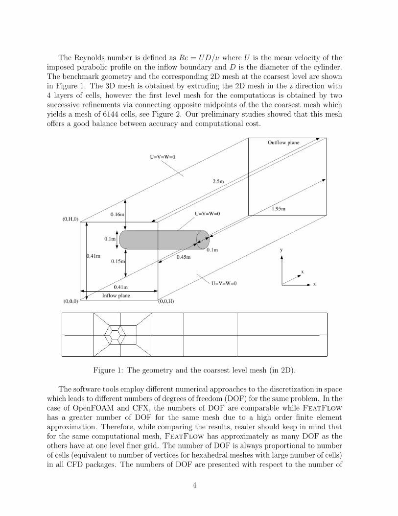
The Reynolds number is defined as Re = UD/ν where U is the mean velocity of theimposed parabolic profile on the inflow boundary and D is the diameter of the cylinder.The benchmark geometry and the corresponding 2D mesh at the coarsest level are shownin Figure 1. The 3D mesh is obtained by extruding the 2D mesh in the z direction with4 layers of cells, however the first level mesh for the computations is obtained by twosuccessive refinements via connecting opposite midpoints of the the coarsest mesh whichyields a mesh of 6144 cells, see Figure 2. Our preliminary studies showed that this meshoffers a good balance between accuracy and computational cost.

Figure 1: The geometry and the coarsest level mesh (in 2D).

The software tools employ different numerical approaches to the discretization in spacewhich leads to different numbers of degrees of freedom (DOF) for the same problem. In thecase of OpenFOAM and CFX, the numbers of DOF are comparable while FeatFlowhas a greater number of DOF for the same mesh due to a high order finite elementapproximation. Therefore, while comparing the results, reader should keep in mind thatfor the same computational mesh, FeatFlow has approximately as many DOF as theothers have at one level finer grid. The number of DOF is always proportional to numberof cells (equivalent to number of vertices for hexahedral meshes with large number of cells)in all CFD packages. The numbers of DOF are presented with respect to the number of

4

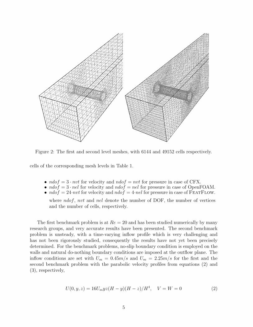
Figure 2: The first and second level meshes, with 6144 and 49152 cells respectively.

cells of the corresponding mesh levels in Table 1.

• ndof = 3 · nvt for velocity and ndof = nvt for pressure in case of CFX.• ndof = 3 · nel for velocity and ndof = nel for pressure in case of OpenFOAM.• ndof = 24·nvt for velocity and ndof = 4·nel for pressure in case of FeatFlow.

where ndof , nvt and nel denote the number of DOF, the number of verticesand the number of cells, respectively.

The first benchmark problem is at Re = 20 and has been studied numerically by manyresearch groups, and very accurate results have been presented. The second benchmarkproblem is unsteady, with a time-varying inflow profile which is very challenging andhas not been rigorously studied, consequently the results have not yet been preciselydetermined. For the benchmark problems, no-slip boundary condition is employed on thewalls and natural do-nothing boundary conditions are imposed at the outflow plane. Theinflow conditions are set with Um = 0.45m/s and Um = 2.25m/s for the first and thesecond benchmark problem with the parabolic velocity profiles from equations (2) and(3), respectively,

U(0, y, z) = 16Umyz(H − y)(H − z)/H4, V = W = 0 (2)

5

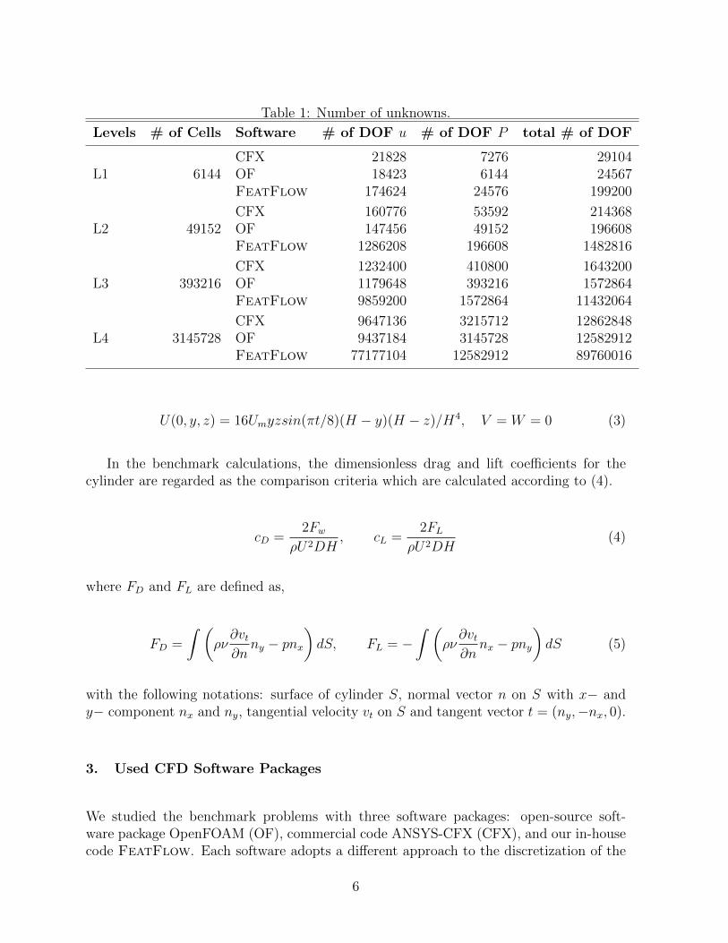
Table 1: Number of unknowns.

Levels # of Cells Software # of DOF u # of DOF P total # of DOF

CFX 21828 7276 29104L1 6144 OF 18423 6144 24567

FeatFlow 174624 24576 199200

CFX 160776 53592 214368L2 49152 OF 147456 49152 196608

FeatFlow 1286208 196608 1482816

CFX 1232400 410800 1643200L3 393216 OF 1179648 393216 1572864

FeatFlow 9859200 1572864 11432064

CFX 9647136 3215712 12862848L4 3145728 OF 9437184 3145728 12582912

FeatFlow 77177104 12582912 89760016

U(0, y, z) = 16Umyzsin(πt/8)(H − y)(H − z)/H4, V = W = 0 (3)

In the benchmark calculations, the dimensionless drag and lift coefficients for thecylinder are regarded as the comparison criteria which are calculated according to (4).

cD =2Fw

ρU2DH, cL =

2FL

ρU2DH(4)

where FD and FL are defined as,

FD =

∫ (ρν∂vt∂n

ny − pnx

)dS, FL = −

∫ (ρν∂vt∂n

nx − pny

)dS (5)

with the following notations: surface of cylinder S, normal vector n on S with x− andy− component nx and ny, tangential velocity vt on S and tangent vector t = (ny,−nx, 0).

3. Used CFD Software Packages

We studied the benchmark problems with three software packages: open-source soft-ware package OpenFOAM (OF), commercial code ANSYS-CFX (CFX), and our in-housecode FeatFlow. Each software adopts a different approach to the discretization of the

6

Navier-Stokes equations. The first adopts a conventional Finite Volume Method (FVM),ANSYS-CFX is developed on an element based FVM (ebFVM) and the last adopts ahigh order Galerkin Finite Element approach. Their approaches to the discretization ofNavier-Stokes equations are one of the main differences between the codes. Moreover,their solution approach to the resulting linear and non-linear systems of equations af-ter discretization is another distinction which influences the computational performancerather than the accuracy of the results. Nevertheless, in the case of our in-house code, thespace discretization method is also effective regarding the performance of the solvers, thefinite element spaces were chosen such that the linear solvers would be the most efficient.

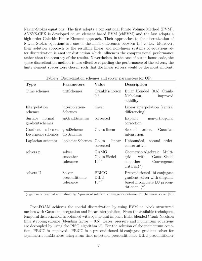
Table 2: Discretization schemes and solver parameters for OF.

Type Parameters Value Description

Time schemes ddtSchemes CrankNicholson0.5

Euler blended (0.5) Crank-Nicholson, improvedstability.

Interpolationschemes

interpolation-Schemes

linear Linear interpolation (centraldifferencing).

Surface normalgradientschemes

snGradSchemes corrected Explicit non-orthogonalcorrection.

Gradient schemesDivergence schemes

gradSchemesdivSchemes

Gauss linear Second order, Gaussianintegration.

Laplacian schemes laplacianSchemes Gauss linearcorrected

Unbounded, second order,conservative.

solvers p solversmoothertolerance

GAMGGauss-Siedel10−7

Geometric-Algebraic Multi-grid with Gauss-Siedelsmoother. Convergencecriteria.(*)

solvers U Solverpreconditionertolerance

PBICGDILU10−6

Preconditioned bi-conjugategradient solver with diagonalbased incomplete LU precon-ditioner. (*)

(L2norm of residual normalized by L2norm of solution, convergence criterion for the linear solver [6].)

OpenFOAM achieves the spatial discretization by using FVM on block structuredmeshes with Gaussian integration and linear interpolation. From the available techniques,temporal discretization is obtained with equidistant implicit Euler blended Crank-Nicolsontime stepping scheme (blending factor = 0.5). Later, pressure and momentum equationsare decoupled by using the PISO algorithm [5]. For the solution of the momentum equa-tion, PBiCG is employed. PBiCG is a preconditioned bi-conjugate gradient solver forasymmetric lduMatrices using a run-time selectable preconditioner. DILU preconditioner

7

which is a simplified diagonal-based incomplete LU preconditioner for asymmetric ma-trices was chosen. Then, the pressure equation is solved by using a Geometric-AlgebraicMultigrid solver with a Gauss-Seidel type smoother. The details of the chosen discretiza-tion schemes and solver tolerances are presented in Table 2.

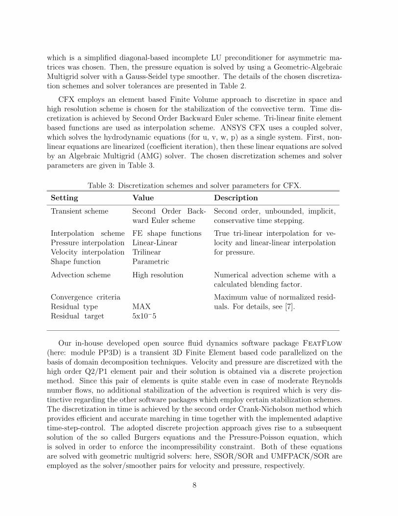
CFX employs an element based Finite Volume approach to discretize in space andhigh resolution scheme is chosen for the stabilization of the convective term. Time dis-cretization is achieved by Second Order Backward Euler scheme. Tri-linear finite elementbased functions are used as interpolation scheme. ANSYS CFX uses a coupled solver,which solves the hydrodynamic equations (for u, v, w, p) as a single system. First, non-linear equations are linearized (coefficient iteration), then these linear equations are solvedby an Algebraic Multigrid (AMG) solver. The chosen discretization schemes and solverparameters are given in Table 3.

Table 3: Discretization schemes and solver parameters for CFX.

Setting Value Description

Transient scheme Second Order Back-ward Euler scheme

Second order, unbounded, implicit,conservative time stepping.

Interpolation schemePressure interpolationVelocity interpolationShape function

FE shape functionsLinear-LinearTrilinearParametric

True tri-linear interpolation for ve-locity and linear-linear interpolationfor pressure.

Advection scheme High resolution Numerical advection scheme with acalculated blending factor.

Convergence criteriaResidual typeResidual target

MAX5x10−5

Maximum value of normalized resid-uals. For details, see [7].

Our in-house developed open source fluid dynamics software package FeatFlow(here: module PP3D) is a transient 3D Finite Element based code parallelized on thebasis of domain decomposition techniques. Velocity and pressure are discretized with thehigh order Q2/P1 element pair and their solution is obtained via a discrete projectionmethod. Since this pair of elements is quite stable even in case of moderate Reynoldsnumber flows, no additional stabilization of the advection is required which is very dis-tinctive regarding the other software packages which employ certain stabilization schemes.The discretization in time is achieved by the second order Crank-Nicholson method whichprovides efficient and accurate marching in time together with the implemented adaptivetime-step-control. The adopted discrete projection approach gives rise to a subsequentsolution of the so called Burgers equations and the Pressure-Poisson equation, whichis solved in order to enforce the incompressibility constraint. Both of these equationsare solved with geometric multigrid solvers: here, SSOR/SOR and UMFPACK/SOR areemployed as the solver/smoother pairs for velocity and pressure, respectively.

8

4. Results

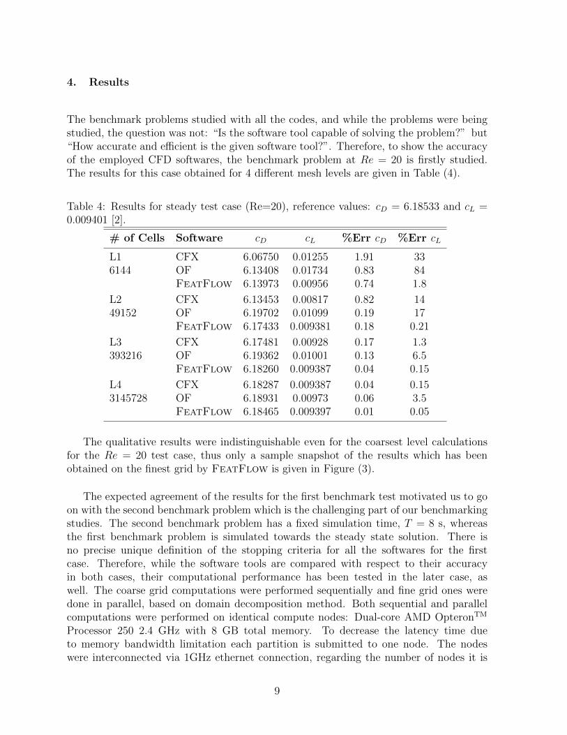
The benchmark problems studied with all the codes, and while the problems were beingstudied, the question was not: “Is the software tool capable of solving the problem?” but“How accurate and efficient is the given software tool?”. Therefore, to show the accuracyof the employed CFD softwares, the benchmark problem at Re = 20 is firstly studied.The results for this case obtained for 4 different mesh levels are given in Table (4).

Table 4: Results for steady test case (Re=20), reference values: cD = 6.18533 and cL =0.009401 [2].

# of Cells Software cD cL %Err cD %Err cL

L1 CFX 6.06750 0.01255 1.91 336144 OF 6.13408 0.01734 0.83 84

FeatFlow 6.13973 0.00956 0.74 1.8

L2 CFX 6.13453 0.00817 0.82 1449152 OF 6.19702 0.01099 0.19 17

FeatFlow 6.17433 0.009381 0.18 0.21

L3 CFX 6.17481 0.00928 0.17 1.3393216 OF 6.19362 0.01001 0.13 6.5

FeatFlow 6.18260 0.009387 0.04 0.15

L4 CFX 6.18287 0.009387 0.04 0.153145728 OF 6.18931 0.00973 0.06 3.5

FeatFlow 6.18465 0.009397 0.01 0.05

The qualitative results were indistinguishable even for the coarsest level calculationsfor the Re = 20 test case, thus only a sample snapshot of the results which has beenobtained on the finest grid by FeatFlow is given in Figure (3).

The expected agreement of the results for the first benchmark test motivated us to goon with the second benchmark problem which is the challenging part of our benchmarkingstudies. The second benchmark problem has a fixed simulation time, T = 8 s, whereasthe first benchmark problem is simulated towards the steady state solution. There isno precise unique definition of the stopping criteria for all the softwares for the firstcase. Therefore, while the software tools are compared with respect to their accuracyin both cases, their computational performance has been tested in the later case, aswell. The coarse grid computations were performed sequentially and fine grid ones weredone in parallel, based on domain decomposition method. Both sequential and parallelcomputations were performed on identical compute nodes: Dual-core AMD OpteronTM

Processor 250 2.4 GHz with 8 GB total memory. To decrease the latency time dueto memory bandwidth limitation each partition is submitted to one node. The nodeswere interconnected via 1GHz ethernet connection, regarding the number of nodes it is

9

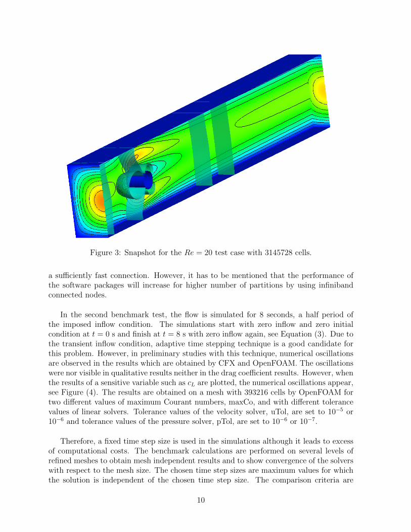
Figure 3: Snapshot for the Re = 20 test case with 3145728 cells.

a sufficiently fast connection. However, it has to be mentioned that the performance ofthe software packages will increase for higher number of partitions by using infinibandconnected nodes.

In the second benchmark test, the flow is simulated for 8 seconds, a half period ofthe imposed inflow condition. The simulations start with zero inflow and zero initialcondition at t = 0 s and finish at t = 8 s with zero inflow again, see Equation (3). Due tothe transient inflow condition, adaptive time stepping technique is a good candidate forthis problem. However, in preliminary studies with this technique, numerical oscillationsare observed in the results which are obtained by CFX and OpenFOAM. The oscillationswere nor visible in qualitative results neither in the drag coefficient results. However, whenthe results of a sensitive variable such as cL are plotted, the numerical oscillations appear,see Figure (4). The results are obtained on a mesh with 393216 cells by OpenFOAM fortwo different values of maximum Courant numbers, maxCo, and with different tolerancevalues of linear solvers. Tolerance values of the velocity solver, uTol, are set to 10−5 or10−6 and tolerance values of the pressure solver, pTol, are set to 10−6 or 10−7.

Therefore, a fixed time step size is used in the simulations although it leads to excessof computational costs. The benchmark calculations are performed on several levels ofrefined meshes to obtain mesh independent results and to show convergence of the solverswith respect to the mesh size. The chosen time step sizes are maximum values for whichthe solution is independent of the chosen time step size. The comparison criteria are

10

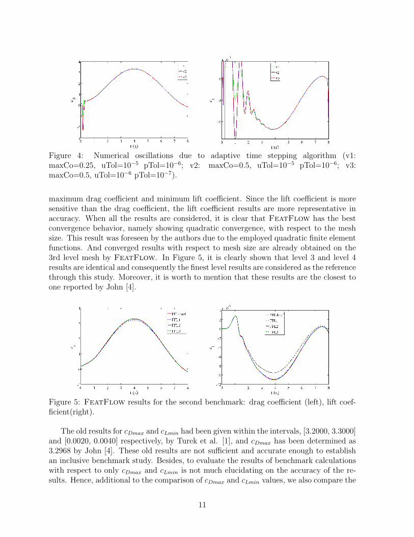
Figure 4: Numerical oscillations due to adaptive time stepping algorithm (v1:maxCo=0.25, uTol=10−5 pTol=10−6; v2: maxCo=0.5, uTol=10−5 pTol=10−6; v3:maxCo=0.5, uTol=10−6 pTol=10−7).

maximum drag coefficient and minimum lift coefficient. Since the lift coefficient is moresensitive than the drag coefficient, the lift coefficient results are more representative inaccuracy. When all the results are considered, it is clear that FeatFlow has the bestconvergence behavior, namely showing quadratic convergence, with respect to the meshsize. This result was foreseen by the authors due to the employed quadratic finite elementfunctions. And converged results with respect to mesh size are already obtained on the3rd level mesh by FeatFlow. In Figure 5, it is clearly shown that level 3 and level 4results are identical and consequently the finest level results are considered as the referencethrough this study. Moreover, it is worth to mention that these results are the closest toone reported by John [4].

Figure 5: FeatFlow results for the second benchmark: drag coefficient (left), lift coef-ficient(right).

The old results for cDmax and cLmin had been given within the intervals, [3.2000, 3.3000]and [0.0020, 0.0040] respectively, by Turek et al. [1], and cDmax has been determined as3.2968 by John [4]. These old results are not sufficient and accurate enough to establishan inclusive benchmark study. Besides, to evaluate the results of benchmark calculationswith respect to only cDmax and cLmin is not much elucidating on the accuracy of the re-sults. Hence, additional to the comparison of cDmax and cLmin values, we also compare the

11

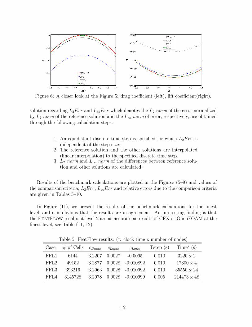
Figure 6: A closer look at the Figure 5: drag coefficient (left), lift coefficient(right).

solution regarding L2Err and L∞Err which denotes the L2 norm of the error normalizedby L2 norm of the reference solution and the L∞ norm of error, respectively, are obtainedthrough the following calculation steps:

1. An equidistant discrete time step is specified for which L2Err isindependent of the step size.

2. The reference solution and the other solutions are interpolated(linear interpolation) to the specified discrete time step.

3. L2 norm and L∞ norm of the differences between reference solu-tion and other solutions are calculated.

Results of the benchmark calculations are plotted in the Figures (5–9) and values ofthe comparison criteria, L2Err, L∞Err and relative errors due to the comparison criteriaare given in Tables 5–10.

In Figure (11), we present the results of the benchmark calculations for the finestlevel, and it is obvious that the results are in agreement. An interesting finding is thatthe FeatFlow results at level 2 are as accurate as results of CFX or OpenFOAM at thefinest level, see Table (11, 12).

Table 5: FeatFlow results. (∗: clock time x number of nodes)

Case # of Cells cDmax cLmax cLmin Tstep (s) Time∗ (s)

FFL1 6144 3.2207 0.0027 -0.0095 0.010 3220 x 2

FFL2 49152 3.2877 0.0028 -0.010892 0.010 17300 x 4

FFL3 393216 3.2963 0.0028 -0.010992 0.010 35550 x 24

FFL4 3145728 3.2978 0.0028 -0.010999 0.005 214473 x 48

12

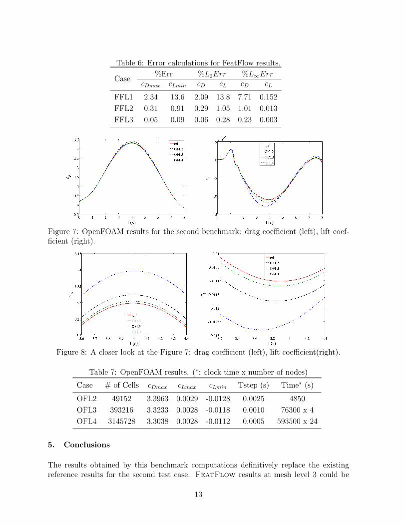
Table 6: Error calculations for FeatFlow results.

Case%Err %L2Err %L∞Err

cDmax cLmin cD cL cD cL

FFL1 2.34 13.6 2.09 13.8 7.71 0.152

FFL2 0.31 0.91 0.29 1.05 1.01 0.013

FFL3 0.05 0.09 0.06 0.28 0.23 0.003

Figure 7: OpenFOAM results for the second benchmark: drag coefficient (left), lift coef-ficient (right).


Table 7: OpenFOAM results. (∗: clock time x number of nodes)


OFL2 49152 3.3963 0.0029 -0.0128 0.0025 4850

OFL3 393216 3.3233 0.0028 -0.0118 0.0010 76300 x 4

OFL4 3145728 3.3038 0.0028 -0.0112 0.0005 593500 x 24

5. Conclusions

The results obtained by this benchmark computations definitively replace the existingreference results for the second test case. FeatFlow results at mesh level 3 could be

13

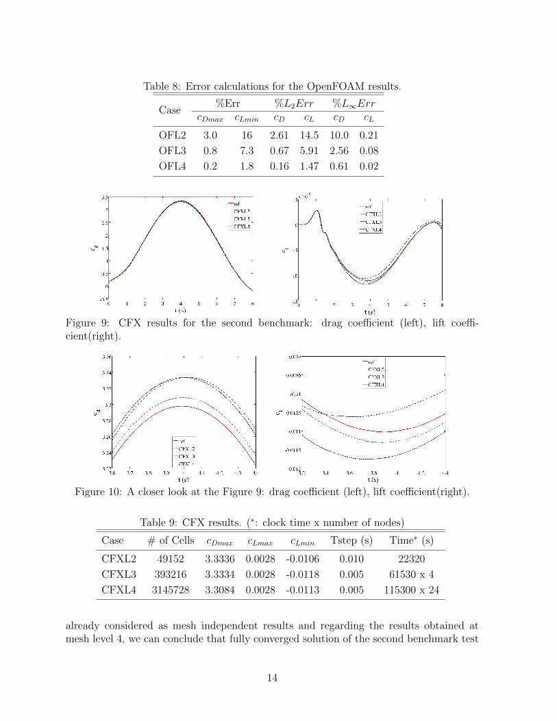
Table 8: Error calculations for the OpenFOAM results.



OFL2 3.0 16 2.61 14.5 10.0 0.21

OFL3 0.8 7.3 0.67 5.91 2.56 0.08

OFL4 0.2 1.8 0.16 1.47 0.61 0.02

Figure 9: CFX results for the second benchmark: drag coefficient (left), lift coeffi-cient(right).


Table 9: CFX results. (∗: clock time x number of nodes)


CFXL2 49152 3.3336 0.0028 -0.0106 0.010 22320

CFXL3 393216 3.3334 0.0028 -0.0118 0.005 61530 x 4

CFXL4 3145728 3.3084 0.0028 -0.0113 0.005 115300 x 24

already considered as mesh independent results and regarding the results obtained atmesh level 4, we can conclude that fully converged solution of the second benchmark test

14

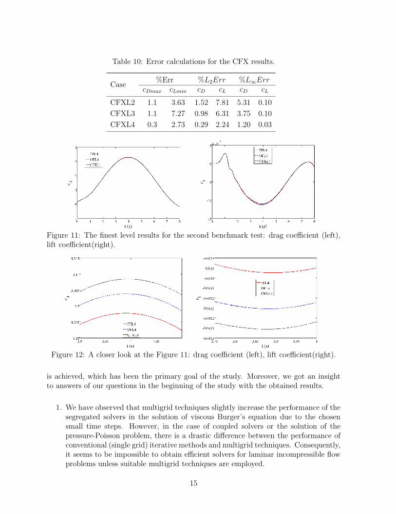
Table 10: Error calculations for the CFX results.



CFXL2 1.1 3.63 1.52 7.81 5.31 0.10

CFXL3 1.1 7.27 0.98 6.31 3.75 0.10

CFXL4 0.3 2.73 0.29 2.24 1.20 0.03

Figure 11: The finest level results for the second benchmark test: drag coefficient (left),lift coefficient(right).


is achieved, which has been the primary goal of the study. Moreover, we got an insightto answers of our questions in the beginning of the study with the obtained results.

1. We have observed that multigrid techniques slightly increase the performance of thesegregated solvers in the solution of viscous Burger’s equation due to the chosensmall time steps. However, in the case of coupled solvers or the solution of thepressure-Poisson problem, there is a drastic difference between the performance ofconventional (single grid) iterative methods and multigrid techniques. Consequently,it seems to be impossible to obtain efficient solvers for laminar incompressible flowproblems unless suitable multigrid techniques are employed.

15

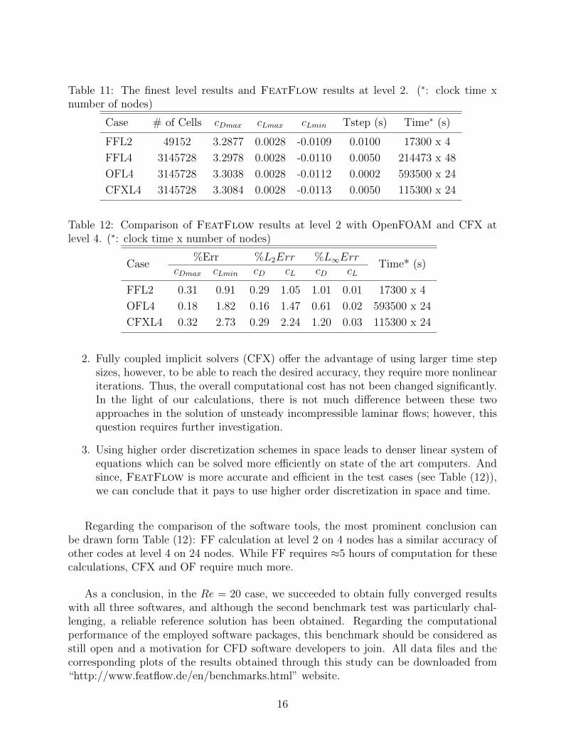
Table 11: The finest level results and FeatFlow results at level 2. (∗: clock time xnumber of nodes)


FFL2 49152 3.2877 0.0028 -0.0109 0.0100 17300 x 4

FFL4 3145728 3.2978 0.0028 -0.0110 0.0050 214473 x 48

OFL4 3145728 3.3038 0.0028 -0.0112 0.0002 593500 x 24

CFXL4 3145728 3.3084 0.0028 -0.0113 0.0050 115300 x 24

Table 12: Comparison of FeatFlow results at level 2 with OpenFOAM and CFX atlevel 4. (∗: clock time x number of nodes)

Case%Err %L2Err %L∞Err Time* (s)


FFL2 0.31 0.91 0.29 1.05 1.01 0.01 17300 x 4

OFL4 0.18 1.82 0.16 1.47 0.61 0.02 593500 x 24

CFXL4 0.32 2.73 0.29 2.24 1.20 0.03 115300 x 24

2. Fully coupled implicit solvers (CFX) offer the advantage of using larger time stepsizes, however, to be able to reach the desired accuracy, they require more nonlineariterations. Thus, the overall computational cost has not been changed significantly.In the light of our calculations, there is not much difference between these twoapproaches in the solution of unsteady incompressible laminar flows; however, thisquestion requires further investigation.

3. Using higher order discretization schemes in space leads to denser linear system ofequations which can be solved more efficiently on state of the art computers. Andsince, FeatFlow is more accurate and efficient in the test cases (see Table (12)),we can conclude that it pays to use higher order discretization in space and time.

Regarding the comparison of the software tools, the most prominent conclusion canbe drawn form Table (12): FF calculation at level 2 on 4 nodes has a similar accuracy ofother codes at level 4 on 24 nodes. While FF requires ≈5 hours of computation for thesecalculations, CFX and OF require much more.

As a conclusion, in the Re = 20 case, we succeeded to obtain fully converged resultswith all three softwares, and although the second benchmark test was particularly chal-lenging, a reliable reference solution has been obtained. Regarding the computationalperformance of the employed software packages, this benchmark should be considered asstill open and a motivation for CFD software developers to join. All data files and thecorresponding plots of the results obtained through this study can be downloaded from“http://www.featflow.de/en/benchmarks.html” website.

16

Acknowledgements

The authors like to thank the German Research Foundation (DFG) for partially sup-porting the work under grants Sonderforschungsbereich SFB708 (TP B7) and SPP1423(Tu102/32-1), and Sulzer Innotec, Sulzer Markets and Technology AG for supportingEvren Bayraktar with a doctoral scholarship.

References

[1] M. Schafer and S.Turek, Benchmark computations of laminar flow around a cylinder(With support by F. Durst, E. Krause and R. Rannacher). In E. Hirschel, editor, FlowSimulation with High-Performance Computers II. DFG priority research programresults 1993-1995, number 52 in Notes Numer. Fluid Mech., pp.547–566. Vieweg,Weisbaden, 1996.

[2] M. Braack and T. Richter, Solutions of 3D Navier-Stokes benchmark problems withAdaptive Finite Elements. Computers and Fluids, 2006, 35(4), pp.372–392.

[3] V.John, Higher order finite element methods and multigrid solvers in a benchmarkproblem for 3D Navier-Stokes equations, Int. J. Numer. Math. Fluids, 2002, 40,pp.755–798.

[4] V.John, On the efficiency of linearization schemes and coupled multigrid methods inthe simulation of a 3D flow around a cylinder, Int. J. Numer. Math. Fluids, 2006,50, pp. 845–862.

[5] J.H Ferziger and M.Peric, Computational Methods for Fluid Dynamics, 3rd ed.Springer, 2002.

[6] OpenFOAM User’s guide (version 1.6), 2009, http://www.openfoam.com/docs/

[7] ANSYS CFX-Solver, Release 10.0:Theory, http://www.ansys.com/cfx

17

benchmark computations of 3d laminar flow around a ... · benchmark computations of 3d laminar flow...

Documents