BENCHMARK RESULTS FOR TESTING ADAPTIVE FINITE ELEMENT

EIGENVALUE PROCEDURES II (CLUSTER ROBUST EIGENVECTOR AND

EIGENVALUE ESTIMATES)

STEFANO GIANI, LUKA GRUBISIC, AND JEFFREY S. OVALL

Abstract. As a model benchmark problem for this study we consider a highly singular transmission typeeigenvalue problem which we study in detail both analytically as well as numerically. In order to justify our

claim of cluster robust and highly accurate approximation of a selected groups of eigenvalues and associated

eigenfunctions, we give a new analysis of a class of direct residual eigenspace/vector approximation estimatesUnlike in the first part of the paper, we now use conforming higher order finite elements, since the canonical

choice of an appropriate norm to measure eigenvector approximation by discontinuous Galerkin methods is

an open problem.

1. Introduction

Accurate computation of eigenvalues and eigenvectors of differential operators defined in planar regionshas attracted considerable attention recently. A central paper in this body of work is the 2005 contributionof Trefethen and Betcke [10] on computing eigenpairs for the Laplacian on a variety of planar domains, bythe method of particular solutions. This approach produced highly accurate eigenvalues—correct to 13 or14 digits in some cases—but the approach is limited in its application scope to differential operators whosehighest order coefficients are constant and lower order coefficients are analytic, see the discussion from [15].In particular this means that handling anisotropic diffusion operators is excluded. For further discussion ofrecent research in this area see [9, 8, 30].

This limitation excludes many interesting eigenvalue model problems for composite materials, such asthose which are of interest for methods of nondestructive sensing (cf. [1, 2]). Our interest in problems ofthis sort is motivated by considerations of photonic crystals and related problems, cf. [3, 16]. Althoughsuch problems are not directly addressed in this work, we do consider examples which have jump discon-tinuities in the coefficients of the highest and lowest order derivatives and therefore capture some of thecomputational difficulties which arise in photonic crystal applications. In [17], we used an hp-adaptive dis-continuous Galerkin method, with duality-based (goal-oriented) adaptive refinement, to efficiently produceeigenvalue approximations having at least 10 correct digits for several model problems, including those withdiscontinuous coefficients.

Our experience thus far indicates that such hp-DG methods provide the most efficient means of computingeigenvalues in the discontinuous-coefficient case in terms of flops-per-correct-digit. However, the structureof DG-methods is such that only limited results are available on the accuracy of computed eigenvectorapproximations. This is, in part, due to the difficulty in choosing an appropriate norm for the analysis. Theanalytical framework that we have developed elsewhere for lower-order continuous elements ([7, 20]) usesnative Hilbert space norms in an essential way, so standard DG norms appear very difficult to incorporatein this kind of analysis.

Motivated by this work on h adaptive finite element approximations we show a way to obtain reliable andefficient a-posteriori estimates in the hp-setting. As is standard for a-posteriori error analysis of eigenvalueproblems, this task is reduced to analysis of associate boundary value problems. Our approach to thisreduction from eigenvalue to boundary value problems is derived from operator-theoretic considerations,and very naturally leads to estimates of both eigenvalue and invariant subspace errors which are robust withrespect to degenerate eigenvalues. The idea to reduce the study of the eigenvalue problem to the study of

Date: November 29, 2013.2000 Mathematics Subject Classification. Primary: 65N30, Secondary: 65N25, 65N15.

Key words and phrases. eigenvalue problems, finite element methods, a posteriori error estimates, hp-apaptivity .

1

the associated boundary value problem is not new. However, the analysis from [7, 20] allows us to explicitlyshow that our bound are independent of the distances between clustered eigenvalues, but rather depend onthe distance to the unwanted component of the spectrum. We obtain estimates which are both reliable aswell as efficient. Furthermore, results from [7] indicate that the influence of the spectral separation is ofhigher order in the norm of the residual.

Because it is straight-forward to apply our framework in the analysis of approximations of eigenvectorsof low regularity, H1+α for some (small) α > 0, as well as invariant subspaces corresponding to degenerateeigenvalues (those having multiplicity greater than one or clustered groups of eigenvalues), it seems usefulto develop a continuous hp-adaptive scheme based on this approach. The aim is that a more robust theorymight soon be complemented with computational efficiency which is competitive with its DG counterpart.The present work is a significant step in that direction.

For more information on hp-adaptive approximation methods for eigenvalue problems see [5, 24, 28]. Thesereferences mostly address a priori analysis of the eigenvalue/vector approximation problem. For a recentcomprehensive treatment of a priori eigenvalue approximation error estimation see [13] and the referencescited therein. For a recent account of a posteriori error analysis of hp-adaptive eigenvalue approximationssee [4].

The rest of this paper is organized as follows. In Section 2 we introduce our model problem and basicnotation related to its continuous and discrete versions, as well as some basic theory related to such eigenvalueproblems. The notion of approximation defects and their relevance is discussed in Section 3, with resultsfrom [7, 20] extended for use in the present context. These extensions make possible the incorporation ofresults from [26, Section 3], which pertain to boundary value problem error estimation, to obtain efficientand reliable estimates of eigenvalue approximations, which is discussed in Section 4. Also in this section wepresent a subspace perturbation type result for the accuracy of eigenvectors—to assess the accuracy of theangle operator we use the Hilbert-Schmidt norm. In Section 4.2 we compare our results with other referencesin the literature. Section 5, which constitutes the bulk of the paper, is devoted to numerical experiments ona variety of different kinds of problems to assess the practical behavior of the proposed approach.

2. Model Problem and Discretization

Let Ω ⊂ R2 be a bounded polygonal domain, possibly with re-entrant corners, and let ∂ΩD ⊂ ∂Ω havepositive (1D) Lebesgue measure. We define the space H = v ∈ H1(Ω) : v|∂ΩD

= 0, where these boundary

values are understood in the sense of trace. We are interested in the eigenvalue problem:

Find (λ, ψ) ∈ R×H so that B(ψ, v) = λ(ψ, v) and ψ 6= 0 for all v ∈ H .(1)

Here we have assumed

(2) B(w, v) =

∫Ω

A∇w · ∇v + cwv dx,

and

(3) (w, v) =

∫Ω

wv dx

is the standard L2 inner-product. We will also assume that the diffusion matrix A is piecewise constant anduniformly positive definite a.e., the scalar c is also piecewise constant and non-negative. These assumptionsare sufficient to guarantee that there are constants β0, β1 > 0 such that B(v, w) ≤ β1‖v‖1‖w‖1 and B[v]

.=

B(v, v) ≥ β0‖v‖21 for all v, w ∈ H. In other words B(·, ·) is an inner product on H, whose induced “energy”-norm ||| · ||| is equivalent to ‖ · ‖1. The numbers β0 and β1 are referred to, respectively, as the coercivity andcontinuity constants for B.

Here and elsewhere, we use the following standard notation for norms and seminorms: for k ∈ N andS ⊂ Ω we denote the standard norms and semi-norms on the Hilbert spaces Hk(S) by

‖v‖2k,S =∑|α|≤k

‖Dαv‖2S |v|2k,S =∑|α|=k

‖Dαv‖2S ,(4)

2

where ‖ · ‖S denotes the L2 norm on S. Additionally, we define ||| · |||S by

|||v|||2S =

∫S

A∇v · ∇v + cv2 dx ,(5)

recognizing that this may be a semi-norm. When S = Ω we omit it from the subscript. Our assumptionson A and c guarantee that there are local constants β0S , γ1S > 0 such that β0S |v|21,S ≤ |||v|||2S ≤ β1S‖v‖21,S ,

and the seminorm in the lower bound can be replaced with the full norm (after modifying β0S if necessary)if c(x) ≥ cS > 0 on S.

2.1. Notational conventions for eigenvalues and eigenvectors. The variational eigenvalue problem(1)–(3) is attained by the positive sequence of eigenvalues

(6) 0 < λ1 ≤ λ2 ≤ · · · ≤ λq ≤ · · ·and the sequence of eigenvectors (ψi)i∈N such that

B(ψi, v) = λi(ψi, v), ∀v ∈ H, and (ψi, ψj) = δij .(7)

Here we have counted the eigenvalues according to their multiplicity and we will also use the notation ψi ⊥ ψjwhen (ψi, ψj) = 0 (when i 6= j). Furthermore, the sequence (λi)i∈N has no finite accumulation point; anddue to the Peron-Frobenius theorem we know that, in the case in which Ω is a path-wise connected domain,the inequality λ1 < λ2 holds and the eigenvector ψ1 can be chosen so that ψ1 is continuous and ψ1 > 0 holdspointwise in Ω. We will also use the notation

SpecB := λi : i ∈ Nto denote the spectrum of the variational eigenvalue problem (7) and we use

M(λ) := spanψ : B(ψ, φ) = λ(ψ, φ), ∀φ ∈ Hto denote the spectral subspace associated to λ ∈ SpecB . For variational eigenvalue problems like (7), whichare defined by the form (2), the subspaces M(λ), λ ∈ SpecB are finite dimensional. Furthermore, let Eλ bethe L2 orthogonal projection onto M(λ). Then ∑

λ∈SpecB

Eλ = I

and the spaces M(λ) = RanEλ and M(µ) = RanEµ are mutually orthogonal for λ, µ ∈ SpecB and λ 6= µ.Finally, note that

B(ψ, φ) =∑

λ∈Spec(A)

λ(ψ,Eλφ), ψ, φ ∈ H

and so we obtain an alternative representation of the energy norm

(8) |||ψ|||2 = B(ψ,ψ) =∑

λ∈Spec(A)

λ(ψ,Eλψ), ψ ∈ H.

2.2. Discrete eigenvalue/eigenvector approximations. We discretize (1) using hp-finite element spaces,which we now briefly describe. Let T = Th be a triangulation of Ω with the piecewise-constant mesh functionh : Th → (0, 1), h(K) = diam(K) for K ∈ Th. Throughout we implicitly assume that the mesh is alignedwith all discontinuities of the data A and c, as well as any locations where the (homogeneous) boundaryconditions change between Dirichlet and Neumann. Given a piecewise-constant distribution of polynomialdegrees, p : Th → N, we define the space

V = V ph = v ∈ H ∩ C(Ω) : v∣∣K∈ Pp(K) for each K ∈ Th ,

where Pj is the collection of polynomials of total degree no greater than j on a given set. Suppressing themesh parameter h for convenience, we also define the set of edges E in T , and distinguish interior edges EI ,and edges on the Neumann boundary EN (if there are any). Additionally, we let T (e) denote the one or twotriangles having e ∈ E as an edge, and we extend p to E by p(e) = maxK∈T (e) p(K). As is standard, weassume that the family of spaces satisfy the following regularity properties on Th and p: There is a constantγ > 0 for which

(C1) γ−1[h(K)]2 ≤ area(K) for K ∈ T ,3

(C2) γ−1(p(K) + 1) ≤ p(K ′) + 1 ≤ γ(p(K) + 1) for adjacent K,K ′ ∈ T , K ∩K ′ 6= ∅.It is really just a matter of notational convenience that a single constant γ is used for all of these upper andlower bounds. The shape regularity assumption (C1) implies that the diameters of adjacent elements arecomparable.

In what follows we consider the discrete versions of (1):

Find (λ, ψ) ∈ R× V such that B(ψ, v) = λ(ψ, v) for all v ∈ V .(9)

We also assume, without further comment, that the solutions are ordered and indexed as in (6), with

(ψi, ψj) = δij . We are interested in assessing approximation errors in collections of computed eigenvaluesand associated invariant subspaces. Let sm = µkmk=1 ⊂ (a, b) be the set of all eigenvalues of B, countingmultiplicities, in the interval (a, b), and let Sm = spanφkmk=1 be the associated invariant subspace, with(φi, φj) = δij . The discrete problem (9) is used to compute corresponding approximations sm = µkmk=1

and Sm = spanφkmk=1, with (φi, φj) = δij .

Remark 2.1. When sm consists of the smallest m eigenvalues, we use the absolute labelling sm = λkmk=1

and Sm = spanψkmk=1 instead of the relative labelling involving (µk, φk); and the analogous statement

holds for the discrete approximations sm and Sm. This distinction is used in some of our results, such asTheorems 3.1 and 3.3.

3. Approximation Defects

3.1. Approximation defects. Let the finite element space V ⊂ H be given and let sm and Sm be theapproximations which are computed from V . We define the corresponding approximation defects as:

η2i (Sm) = max

S⊂SmdimS=m−i+1

minf∈Sf 6=0

|||u(f)− u(f)|||2

|||u(f)|||2,(10)

where u(f) and u(f) satisfy the boundary value problems:

B(u(f), v) = (f, v) for every v ∈ H(11)

B(u(f), v) = (f, v) for every v ∈ V .(12)

In Theorems 3.1 and 3.3 below, we state key theorems from [20, 7], which show that these approximationdefects would yield ideal error estimates for eigenvalue and eigenvector computation if they could becomputed. This motivates the use of a posteriori error estimation techniques for boundary value problemsto efficiently and reliably estimate approximation defects. In [20, 7], we used hierarchical bases to estimatethe approximation defects when V was the space of continuous, piecewise affine functions. In Section 4 weshow how to utilize the theory of residual based estimates for hp-finite elements from [26] in a similar fashion.

The following result concerns approximations sm and Sm of the (complete) lower part of the spectrum.This is the reason why we have capitalized the dimension parameter m ∈ N, which is associated to the clusterof lowermost eigenvalues, as opposed to a given cluster of eigenvalues contained in the interval

(a, b).

Theorem 3.1. Assume that λm < λm+1, and let Sm be the span of first m ∈ N eigenvectors of (9). If

Sm = spanψ1, · · · , ψM is such that ηm(Sm)

1−ηm(Sm)< λm+1−λm

λm+1+λmthen

(13)λ1

2λm

m∑i=1

η2i (Sm) ≤

m∑i=1

λi − λiλi

≤ CM

m∑i=1

η2i (Sm).

The constant CM depends solely on the relative distance to the unwanted component of the spectrum (e.g.λM−λM+1

λM+λM+1).

The constant CM is given by an explicit formula which is a reasonable practical overestimate, see [20, 7]for details. A similar result holds for the eigenvectors. We point the interested reader to [20, Theorem 4.1and equation (3.10)] and [7, Theorem 3.10].

4

Remark 3.2. Although λ1 < λ2 for the particular problems we consider numerically in the present work,much of the theory carries over to problems where Ω is not pathwise connected, or the boundary conditionsare periodic (as examples). In these cases the Peron-Frobenius theorem does not apply, and it is quitepossible that the smallest eigenvalue is degenerate. If this is the case, and λ1 = λm, then the constant

λ1/2λm in (13) can be replaced by 1.

An important feature of these ideal estimates is that they are asymptotically exact, both as eigenvectoras well as as eigenvalue estimators, as the following theorem indicates in the case of a single degenerateeigenvalue and its corresponding invariant subspace.

Theorem 3.3. Let λq be a degenerate eigenvalue of multiplicty m, λq−1 < λq = λq+m−1 < λq+m. Let Sm =

Sm(T ) = span(φk) ⊂ V = V (T ) be the computed approximation of the invariant subspace corresponding to

λq. Then, taking the pairing of eigenvectors φi and Ritz vectors φi as in [20], we have

limh→0

∑mi=1

|µi−λq|µi∑m

i=1 η2i (Sm)

= 1 , limh→0

∑mi=1

B[φi−φi]B[φi]∑m

i=1 η2i (Sm)

= 1 .(14)

3.2. A relationship with the residual estimates for a Ritz vector basis. This section addresses theissue of the computability of ηi(Sm) by relating these quantities to the standard dual energy norm estimates

of the residuals associated to the Ritz vector basis of Sm.In our notation the energy norm was denoted by ||| · ||| and we use u(·) and u(·) to denote the solution

operators from (11) and (12). We assume φ1, . . . , φm are the Ritz vectors from Sm, then for i, j = 1, . . . ,m,we define the matrices

Eij = B(u(φi)− u(φi), u(φj)− u(φj)

)(15)

Gij = B(u(φi), u(φj)

).(16)

These matrices were introduced in [20] under the name of the error and the gradient matrix. It was shown

in [20] that ηi(Sm) = λi(E,G), where λ1(E,G) ≤ · · · ≤ λm(E,G) are the eigenvalues of the generalizedeigenproblem for the matrix pair (E,G). Furthermore, since G is a positive definite matrix it also holds

that ηi(Sm) = λi(E,G) = λi(G−1/2EG−1/2), where λ1(G−1/2EG−1/2) ≤ · · · ≤ λm(G−1/2EG−1/2) are the

eigenvalues of the matrix G−1/2EG−1/2.

We further assume that φi, i = 1, · · · ,m are among the Ritz vectors from the finite element subspace V ,

V ⊃ Sm from (12). The identity (15) implies that E is a Gram matrix for the set of vectors u(φi)− u(φi),

i = 1, . . . ,m. If we assume that Sm does not contain any eigenvectors, then we conclude that E must bepositive definite matrix. Furthermore, it always holds

η2i (Sm) = λi(G

−1/2EG−1/2)

Eii = µ−2i |||u(µiφi)− u(µiφi)|||2, i = 1, . . . ,m(17)

Dµ ≤ G ≤ (1 + Dl)Dµ,

where Dµ = diag(µ−11 , . . . , µ−1

m ) and Dl = ‖D−1/2µ (G−Dµ)D

−1/2µ ‖. Let us note that Dl is a relative estimate,

so it is expected that even for very crude finite element spaces V we have Dl < 1.We now compute

m∑i=1

λi(D−1/2µ ED−1/2

µ ) = trace(D−1/2µ ED−1/2

µ ) =

m∑i=1

Eiiµi,

and so conclude that

1

1 + Dl

m∑i=1

Eiiµi ≤m∑i=1

η2i (Sm) ≤

m∑i=1

Eiiµi .(18)

We summarize these considerations — using the identity (17) — in the following lemma.5

Lemma 3.4. It holds that

1

1 + Dl

m∑i=1

µ−1i |||u(µiφi)− u(µiφi)|||2 ≤

m∑i=1

η2i (Sm) ≤

m∑i=1

µ−1i |||u(µiφi)− u(µiφi)|||2 .(19)

4. hp-Error Estimation and Adaptivity in the Eigenvalue Context

Using Lemma 3.4, we have reduced the problem of estimating the approximation defects, and hencethe error in our eigenvalue/eigenvector computations, to that of estimating error in associated boundary

value problems. In particular, we must estimate |||u(µiφi) − u(µiφi)|||2 for each Ritz vector, where Sm =

spanφ1, . . . , φm is our approximation of Sm = spanφ1, . . . , φm. We modify key results from [26], which

were stated only for the Laplacian, to our context. The identity u(µiφi) = φi, makes our job easier. Wedefine the element residuals Ri for K ∈ T , and the edge (jump) residuals ri for e ∈ E , by

Ri|K = µiφi − cφi +∇ ·A∇φi ,(20)

ri|e =

−(A∇φi)|K · nK − (A∇φi)|K′ · nK′ , e ∈ EI−(A∇φi)|K · nK , e ∈ EN

.(21)

For interior edges e ∈ EI , K and K ′ are the two adjacent elements, having outward unit normals nK andnK′ , respectively; and for Neumann boundary edges e ∈ EN (if there are any), K is the single adjacentelement, having outward unit normal nK . We note that R is a polynomial of degree no greater than p(K)on K, and r is a polynomial of degree no greater than p(e) on e.

Our estimate of ε2i =

∑K∈T ε

2i (K) ≈ |||u(µiφi)− u(µiφi)|||2 is computed from local quantities,

ε2i (K) =

(h(K)

p(K)

)2

‖Ri‖20,K +1

2

∑e∈EI(K)

h(e)

p(e)‖ri‖20,e +

∑e∈EN (K)

h(e)

p(e)‖ri‖20,e ,(22)

where EI(K) and EN (K) denote the interior edges and Neumann boundary edges of K, respectively. Aninspection the proof of [26, Lemma 3.1] (which was stated for the Laplacian) makes the following assertionclear.

Lemma 4.1. There is a constant C > 0 depending only on the hp-constant γ and the coercivity constant

β0, such that |||u(µiφi)− u(µiφi)|||2 ≤ Cε2i .

A few remarks are in order concerning the lemma above and how it relates to [26, Lemma 3.1]. First, thebound in [26, Lemma 3.1] includes an additional term involving the difference between the righthand side (inour case φi) and its projection on K into a space of polynomials. This additional term only arises in theirresult because they have chosen to use the projection of the righthand side, instead of the righthand sideitself, to define the element residual (here called Ri). They do this in order to employ certain polynomialinverse estimates, which hold in our case outright because our righthand sides are piecewise polynomial.Their result also involves a parameter α ∈ [0, 1], which we have taken to be 0. The result [26, Lemma3.1] is based on Scott-Zhang type quasi-interpolation, which naturally gives rise to errors measured in H1.Mimicking their arguments with our indicator, one would arrive at a result of the form

|||u(µiφi)− u(µiφi)||| ≤ Cεi‖u(µiφi)− u(µiφi)‖1 ,

where C depends only on γ. The constant in the coercivity bound β0‖v‖21 ≤ |||v|||2 enters Lemma 4.1 at thisfinal stage. Similarly, a careful reading of the proofs of [26, Lemma 3.4 and 3.5] show that their efficiencyresults are readily extended to elliptic operators of the type considered here.

Lemma 4.2. For any ε > 0, there is a constant c = c(ε) > 0 depending only on the hp-constant γ and the

global continuity constant β1, such that ε2i (K) ≤ cp2+2ε

K |||u(µiφi)− u(µiφi)|||2ωK.

Here, ωK is the patch of elements which share an edge with K. The global continuity constant β1 could bereplaced in Lemma 4.2 by a local continuity constant β1ωK

if desired.6

Remark 4.3. The p-dependence in local efficiency bound of Lemma 4.2 is unfortunately unavoidable in theproof, and would suggest decreased efficiency of the estimator as pK is increased if this estimate were sharp.Our numerical experiments do seem to indicate that there may be a modest decrease in the efficiency of theestimator under hp-refinement in practical computations.

With these results we now state the main theorem.

Theorem 4.4. Under the assumptions of Theorem 3.1, we have the following upper- and lower-bounds oneigenvalue error,

(23) C1

m∑i=1

λ−1i ε2

i ≤m∑i=1

λi − λiλi

≤ C2

m∑i=1

λ−1i ε2

i .

The constant C1 depends solely on the ratio λ1/(2λM), the hp-regularity constant γ, the continuity constantβ1, and the maximal polynomial degree p = maxK∈T p(K). The constant C2 depends solely on the relativedistance to the unwanted component of the spectrum, the hp-regularity constant γ and the coercivity constantβ0.

Proof. These assertions follow directly from Theorem 3.1, Lemma 3.4, and Lemmas 4.1 and 4.2.

Remark 4.5. It is relative local indicators µ−1i ε2

i (K) which will be used to mark elements for refinement,as will be described in Section 5.

4.1. Eigenvector estimates. A similar result holds for the eigenvectors and eigenspaces. Let now

E(λm) =∑

λ≤λm, λ∈SpecB

Eλ

be the L2 orthogonal projection onto the eigenspace belonging to the first m eigenvalues of the form B asgiven in Theorem 4.4. Let also ‖ · ‖S2

be the Hilbert-Schmidt norm on the ideal of all Hilbert-Schmidtoperators, see [29]. Note that we are considering subsets of the space of bounded (compact) operators fromL2 to L2. In the matrix analysis the Hilblert-Schmidt norm is known as the Frobenius norm and it can beexpressed as ‖A‖S2

=√

trace(A∗A), where we have assumed that A is such that trace(A∗A) is finite. Wenow have the subspace approximation result.

Theorem 4.6. Let Sm = Sm(T ) = span(φk) ⊂ V = V (T ) be the computed approximation of the invariant

subspace corresponding to λi, i = 1, · · · ,m and let P (T ) be the L2 orthogonal projection onto Sm(T ). If theassumptions of Theorem 3.1 hold. Then

(24) ‖E(λm)− P (T )‖S2≤ Cm,T

√√√√ m∑i=1

λ−1i ε2

i .

The constant Cm,T depends solely on the relative distance to the unwanted component of the spectrum (e.g.λM−λm+1

λm+λM+1), the hp-regularity constant γ and the continuity constant β1.

Proof. The conclusion follows readily from [19, Theorem 4.2] and Lemmas 3.4 and 4.1.

This result is a robust reliability estimate which ensures the convergence of invariant subspaces. Withadditional information on eigenvalue separation we present more detailed efficiency and reliability estimatein an eigenvector setting. Let λ1 = λs1 < · · · < λsk be all elements of the set λi : i = 1, · · · ,m. We definethe following gap measure

Gapm := maxi 6=j

λsi + λsj|λsi − λsj |

.

Theorem 4.7. Let ψi and ψi ∈ V ph , i = 1, · · · ,m be eigenvectors and Ritz vectors which satisfy both the

assumptions of Theorem 3.1 and the paring of Theorem 3.3, that is let ηm(Sm) < 1/2 minGapm,λM+λM+1

λM−λM+1.

Then there exist constants CV and cV such that

cV

m∑i=1

λ−1i ε2

i ≤m∑i=1

B[ψi − ψi]B[ψi]

≤ CV

m∑i=1

λ−1i ε2

i .

7

The constant cV depends solely on the ratio λ1/(2λ2), the hp-regularity constant γ, the continuity constantβ1, and the maximal polynomial degree p = maxK∈T p(K). The constant CV depends solely on the relativedistance to the unwanted component of the spectrum, the hp-regularity constant γ and the coercivity constantβ0.

Proof. Let us assume that

ηm(Sm) < 1/2 minGapm,λM + λM+1

λM − λM+1.

Then according to [18, Theorem 6.2] and [20, Proposition 2.5] we may chose eigenvectors ψi and Ritz vectors

ψi, i = 1, · · · ,m such that the paring of Theorem 3.3 holds for every λsi , i = 1, · · · , k. Using [20, Proposition2.5] and [7, Section 4.1] we establish, using the notation from [7, Section 4.1], the estimate

λ1

2λm

m∑i=1

η2i (Sm) ≤

m∑i=1

B[ψi − ψi]B[ψi]

≤ 2 GapmCvec

m∑i=1

η2i (Sm).

The conclusion of the theorem now follows from Lemmas 3.4, 4.1 and 4.2.

4.2. Further references and concluding remarks. Let us close the theoretical part of the paper bymaking some comparisons with other works in the literature. Our a posteriori error estimator is based onthe consideration of the associated boundary value problems (11) and (12) and so we are able to naturallyrelate our error estimation technique to the results on the boundary value problem error estimator from [26].Any improvement in the analysis of the boundary value approximation error estimator will readily lead tothe improvement of our estimator.

A further claim to this end are results like Theorem 3.3 which indicate that the underlying ideal contin-uous eigenvalue approximation error estimator is asymptotically exact. The computable error estimator ε2

i

is expected to better replicate its behavior as asymptotically sharper estimators of the associated bound-ary value problem become available. Our eigenvalue/eigenvector estimation frameworks is such that anyboundary value error estimator can be readily included providing a result like Lemmas 4.1 and 4.2 exist.

A similar eigenvalue/eigenvector approximation error estimator, also based on the estimator from [26],has been presented in [4]. In comparison we provide a more robust analysis of the reliability of the eigen-value/eigenvector estimator (results from [4] were primarily for single eigenvalues, cf [4, Proposition 3.1]).Furthermore, our analysis provides error estimates for the multiple and clustered eigenvalues where stabilityof the estimates depends only on the separation of a multiple eigenvalue (cluster of eigenvalues) from therest of the spectrum. Note that multiple or clustered eigenvalues appear as result of symmetries or nearsymmetries of the problem and are a typical feature of 2D or 3D eigenvalue problems.

As has been pointed out in [4], lower (the so called efficiency) estimates of the error are still suboptimal(cf. Remark 4.3 and the lower estimate cV from Theorem 4.7) in the sense that the lower “error equivalence”constants depend on the maximal polynomial degree of the approximating hp finite element space. As aconsequence, we do not use our estimator to decide on the p refinement. To decide on the choice betweenh and p refinements we use the technique of estimating the local analyticity of the solution as described in[14, 21], for further discussion see Section 5.

5. Benchmarks

In the numerical experiments we illustrate the efficiency of the estimator (23) on several problems of thegeneral form

Lψ = λψ in Ω , ‖ψ‖ = 1 ,(25)

for a second-order, linear elliptic operator L, where homogeneous Dirichlet or Neumann conditions areimposed on the boundary. We then proceed to give benchmark results for eigenvalues which are accompaniedby the eigenvector approximation estimates. We do not report timing, since a discontinuous Galerkin methodis mostly computationally more efficient at the expense of less robust error estimation theory.

Following [6], we assume an error model of the form

λi = λi + Ce−2α√

DOFs

8

for problems whose eigenvectors are expected to be smooth, and

λi = λi + Ce−2α3√

DOFs,

for problems such as those on non-convex polygonal domains and/or discontinuous coefficients, whose eigen-vectors are expected to have isolated singularities. We use DOFs = dim(V pk ) to denote the size of thediscrete problem. The constants C and α are determined by least-squares fitting, and α is reported for eachproblem. Plots are given of the total relative error, its a posteriori estimate, and the associated effectivityindex, shown, respectively, below:

m∑i=1

λi − λiλi

,

m∑i=1

λ−1i ε2

i ,

∑mi=1

λi−λi

λi∑mi=1 λ

−1i ε2

i

.

In the case of a single eigenvalue λi the effectivity index reduces (λi − λi)/ε2i , and we make the following

comparison with what is presented in [4], in which hp-adaptivity is also used for eigenvalue problems. Theeffectivities reported in [4] are in terms of eigenfunction error, which corresponds closely with the squareroot of the effectivities reported here. This difference should be taken into consideration when comparing theeffectivities reported here with those in [4] or other similar contributions. For problems in which the exacteigenvalues are known, we use these values in our error analysis. For most problems, we use highly accuratecomputations on very large problems to produce “exact eigenvalues” for our comparisons, as discussed inthe introduction.

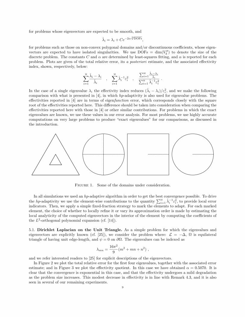
Figure 1. Some of the domains under consideration.

In all simulations we used an hp-adaptive algorithm in order to get the best convergence possible. To drive

the hp-adaptivity we use the element-wise contributions to the quantity∑mi=1 λ

−1i ε2

i , to provide local errorindicators. Then, we apply a simple fixed-fraction strategy to mark the elements to adapt. For each markedelement, the choice of whether to locally refine it or vary its approximation order is made by estimating thelocal analyticity of the computed eigenvectors in the interior of the element by computing the coefficients ofthe L2-orthogonal polynomial expansion (cf. [14]).

5.1. Dirichlet Laplacian on the Unit Triangle. As a simple problem for which the eigenvalues andeigenvectors are explicitly known (cf. [25]), we consider the problem where: L = −∆, Ω is equilateraltriangle of having unit edge-length, and ψ = 0 on ∂Ω. The eigenvalues can be indexed as

λmn =16π2

9(m2 +mn+ n2) ,

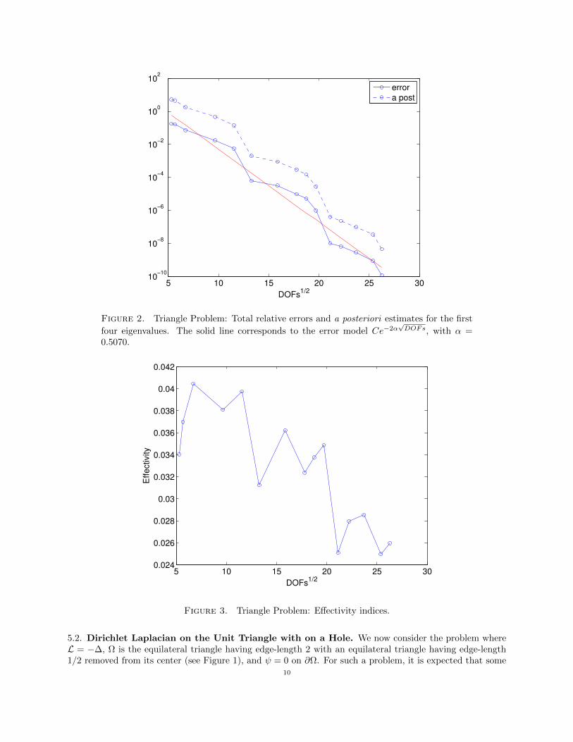
and we refer interested readers to [25] for explicit descriptions of the eigenvectors.In Figure 2 we plot the total relative error for the first four eigenvalues, together with the associated error

estimate; and in Figure 3 we plot the effectivity quotient. In this case we have obtained α = 0.5070. It isclear that the convergence is exponential in this case, and that the effectivity undergoes a mild degradationas the problem size increases. This modest decrease in effectivity is in line with Remark 4.3, and it is alsoseen in several of our remaining experiments.

9

5 10 15 20 25 3010

−10

10−8

10−6

10−4

10−2

100

102

DOFs1/2

error

a post

Figure 2. Triangle Problem: Total relative errors and a posteriori estimates for the first

four eigenvalues. The solid line corresponds to the error model Ce−2α√DOFs, with α =

0.5070.

5 10 15 20 25 300.024

0.026

0.028

0.03

0.032

0.034

0.036

0.038

0.04

0.042

DOFs1/2

Effectivity

Figure 3. Triangle Problem: Effectivity indices.

5.2. Dirichlet Laplacian on the Unit Triangle with on a Hole. We now consider the problem whereL = −∆, Ω is the equilateral triangle having edge-length 2 with an equilateral triangle having edge-length1/2 removed from its center (see Figure 1), and ψ = 0 on ∂Ω. For such a problem, it is expected that some

10

5 10 15 20 25 30 35 4010

−7

10−6

10−5

10−4

10−3

10−2

10−1

100

101

DOFs1/3

error

a post

Figure 4. Triangle with Hole: Total relative errors and a posteriori estimates for the first

three eigenvalues. The solid line corresponds to the error model Ce−2α3√DOFs, with α =

0.2190

5 10 15 20 25 30 35 400.03

0.035

0.04

0.045

0.05

0.055

0.06

0.065

0.07

0.075

DOFs1/3

Effectivity

hp

Figure 5. Triangle with Hole: Effectivity indices

of the eigenvectors will have an r3/5-type singularity at each of the three interior corners, where r is thedistance to the nearest corner. In this case, the exact eigenvalues are unknown, so we computed the followingreference values of them on a very large problem: 40.4650426 for the first eigenvalue and 43.4868466 for thesecond and third, which form a double eigenvalue. These values are accurate at least up to 1e-6.

11

In Figure 4 we plot the relative error and error estimates together, for the first three eigenvalues, and inFigures 5 we plot the corresponding values of the effectivity quotient. We again see exponential convergencewith α = 0.2190 and a modest deterioration of effectivity.

5.3. Square Domain with Discontinuous Reaction Term. For this pair of problems we take Ω =(0, 1)2, ∇ψ · n = 0 on ∂Ω, and Lψ = −∆ψ + κVMD · ψ, where VMD is the characteristic function of thetouching squares labelled M1 in Figure 6. We consider two values of the constant parameter, κ = 10, 100.It is straightforward to see that the corresponding bilinear form is an inner-product in this case (no zeroeigenvalues), and that all eigenvectors are at least in H2.

M2

M2

M1

M1

Figure 6. A modification of the touching squares example of M. Dauge.

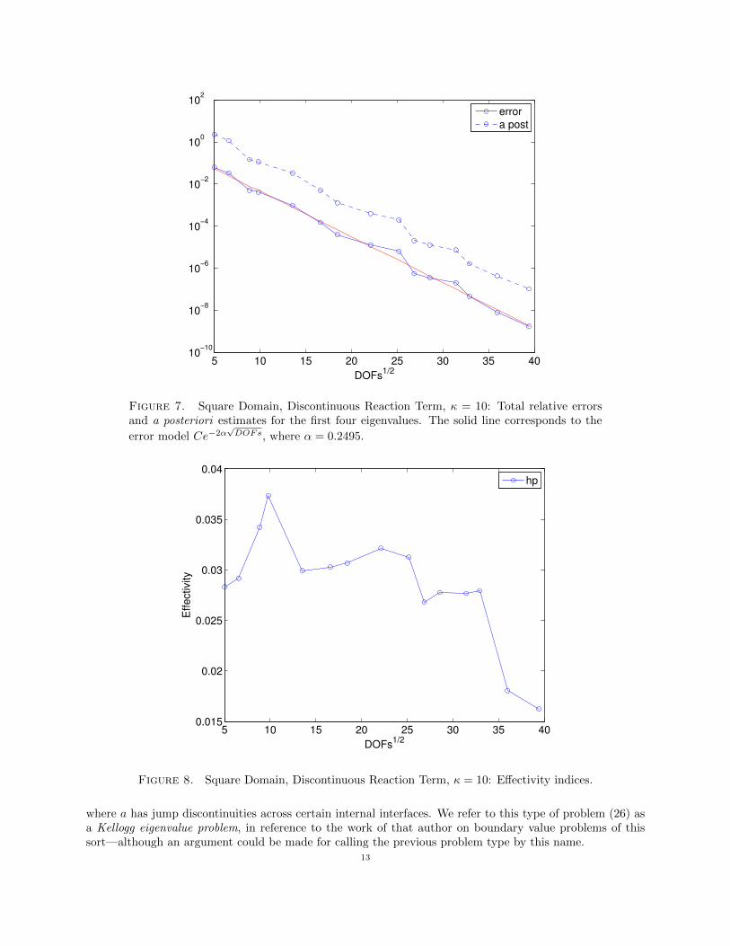
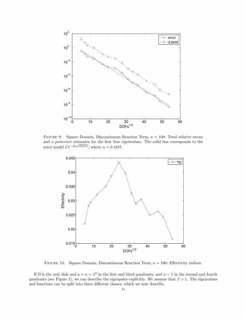
For κ = 10, we have in Figure 7 the total relative error and error estimates for the first four eigenvalues;and the effectivity quotient is given in Figure 8. For these simulations we used the following referencevalues for the first four eigenvalues, which are 1e-8 accurate: 4.150242455, 10.706070962, 18.779725462,25.150325247. The analogous plots for the first four eigenvalues in the case κ = 100 are given in Figure 9and Figure 10. For these simulations, we used the following reference values for the first four eigenvalues,which are 1e-8 accurate: 13.210576406, 13.990033964, 60.294151672, 64.840268299. In both cases we seeapparent exponential convergence with α = 0.2495 and α = 0.1827 respectively, and reasonable effectivitybehavior. It is clear from the error plots that for both values of κ the convergence is exponential.

5.4. Square Domain with Discontinuous Diffusion Term. Using the domain Ω = (0, 1)2, partitionedinto regions M1 and M2 as in Figure 6, and homogeneous Dirichlet conditions ψ = 0 on ∂Ω, we considerthe operator L = −∇ · (a∇), where a = 1 in M2 and a = κ in M1. Such problems can have arbitrarily badsingularities at the cross-point of the domain depending on the relative sizes of a in the two subdomains—see,for example, [22, 23, 11, 12] and [27, Example 5.3].

We have considered two values for κ in M1: 10 and 100. Since the exact eigenvalues are not available,we computed the following three reference values for the first three eigenvalues when κ = 10: 64.226529416,75.028156269, 141.161506328; and the following three reference values for the first three eigenvalues whenκ = 100: 77.800981966, 78.564198245, 193.916538067. All reference values are at least 1e-8 accurate. Therelative error and effectivity plots for both cases are given in Figures 11-14, and again we see apparentexponential convergence with α = 0.5630 and α = 0.5669 respectively. Moreover in Figure 15 we reportedthe final mesh and the final distribution of polynomials orders for κ = 100.

5.5. A Kellogg Problem. We here consider a variant of the previous problem type for which we can givemore specific information about the kinds of singularities which can be expected in terms of the size of thejump discontinuity. More specifically, we consider problems of the form

(26)

∫Ω

a∇ψ · ∇v dx = λ

∫Ω

aψv dx ,

12

5 10 15 20 25 30 35 4010

−10

10−8

10−6

10−4

10−2

100

102

DOFs1/2

error

a post

Figure 7. Square Domain, Discontinuous Reaction Term, κ = 10: Total relative errorsand a posteriori estimates for the first four eigenvalues. The solid line corresponds to the

error model Ce−2α√DOFs, where α = 0.2495.

5 10 15 20 25 30 35 400.015

0.02

0.025

0.03

0.035

0.04

DOFs1/2

Effectivity

hp

Figure 8. Square Domain, Discontinuous Reaction Term, κ = 10: Effectivity indices.

where a has jump discontinuities across certain internal interfaces. We refer to this type of problem (26) asa Kellogg eigenvalue problem, in reference to the work of that author on boundary value problems of thissort—although an argument could be made for calling the previous problem type by this name.

13

0 10 20 30 40 50 6010

−10

10−8

10−6

10−4

10−2

100

102

DOFs1/2

error

a post

Figure 9. Square Domain, Discontinuous Reaction Term, κ = 100: Total relative errorsand a posteriori estimates for the first four eigenvalues. The solid line corresponds to the

error model Ce−2α√DOFs, where α = 0.1827.

0 10 20 30 40 50 600.015

0.02

0.025

0.03

0.035

0.04

0.045

DOFs1/2

Effectivity

hp

Figure 10. Square Domain, Discontinuous Reaction Term, κ = 100: Effectivity indices.

If Ω is the unit disk and a = κ = β2 in the first and third quadrants, and a = 1 in the second and fourthquadrants (see Figure 1), we can describe the eigenpairs explicitly. We assume that β > 1. The eigenvaluesand functions can be split into three different classes, which we now describe.

14

4 6 8 10 12 14 16 18 20 2210

−10

10−8

10−6

10−4

10−2

100

102

DOFs1/3

error

a post

Figure 11. Square Domain, Discontinuous Diffusion Term, κ = 10: Total relative errorsand a posteriori estimates for the first three eigenvalues. The solid line corresponds to the

error model Ce−2α3√DOFs, where α = 0.5630.

0 5 10 15 20 250.005

0.01

0.015

0.02

0.025

0.03

0.035

0.04

0.045

0.05

DOFs1/3

Effectivity

hp

Figure 12. Square Domain, Discontinuous Diffusion Term, κ = 10: Effectivity indices.

Class 1. For k ≥ 0 and m ≥ 1, let z(1)km be the mth positive root of the first-kind Bessel function J2k. The

eigenvalues of this class are λ(1)km = (z

(1)km)2, and each of them, with the exception of those for k = 0, are

15

4 6 8 10 12 14 16 18 20 2210

−10

10−8

10−6

10−4

10−2

100

102

DOFs1/3

error

a post

Figure 13. Square Domain, Discontinuous Diffusion Term, κ = 100: Total relative errorsand a posteriori estimates for the first three eigenvalues. The solid line corresponds to the

error model Ce−2α3√DOFs, where α = 0.5669.

0 5 10 15 20 250

0.005

0.01

0.015

0.02

0.025

0.03

0.035

0.04

DOFs1/3

Effe

ctivity

hp

Figure 14. Square Domain, Discontinuous Diffusion Term, κ = 100: Effectivity indices.

double-eigenvalues. The corresponding eigenvectors are

ψ(1)km = J2k(z

(1)kmr) cos(2kθ) , Ψ

(1)km = a−1/2J2k(z

(1)kmr) sin(2kθ) .

16

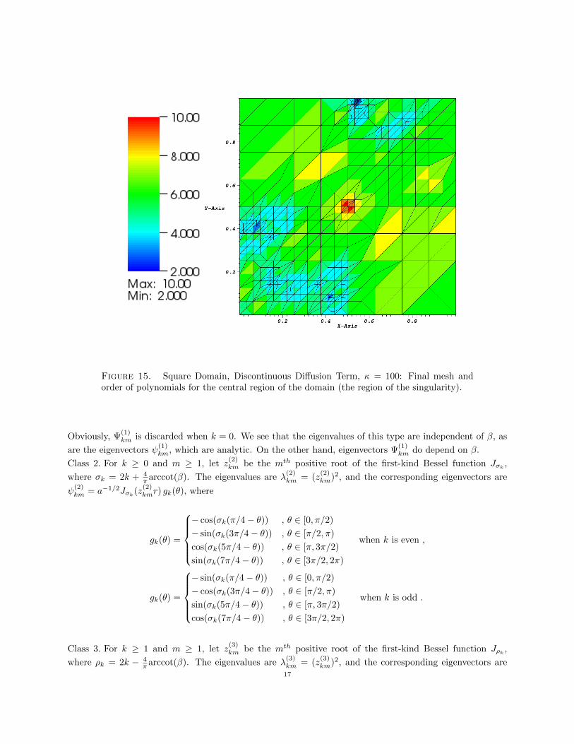
Figure 15. Square Domain, Discontinuous Diffusion Term, κ = 100: Final mesh andorder of polynomials for the central region of the domain (the region of the singularity).

Obviously, Ψ(1)km is discarded when k = 0. We see that the eigenvalues of this type are independent of β, as

are the eigenvectors ψ(1)km, which are analytic. On the other hand, eigenvectors Ψ

(1)km do depend on β.

Class 2. For k ≥ 0 and m ≥ 1, let z(2)km be the mth positive root of the first-kind Bessel function Jσk

,

where σk = 2k + 4πarccot(β). The eigenvalues are λ

(2)km = (z

(2)km)2, and the corresponding eigenvectors are

ψ(2)km = a−1/2Jσk

(z(2)kmr) gk(θ), where

gk(θ) =

− cos(σk(π/4− θ)) , θ ∈ [0, π/2)

− sin(σk(3π/4− θ)) , θ ∈ [π/2, π)

cos(σk(5π/4− θ)) , θ ∈ [π, 3π/2)

sin(σk(7π/4− θ)) , θ ∈ [3π/2, 2π)

when k is even ,

gk(θ) =

− sin(σk(π/4− θ)) , θ ∈ [0, π/2)

− cos(σk(3π/4− θ)) , θ ∈ [π/2, π)

sin(σk(5π/4− θ)) , θ ∈ [π, 3π/2)

cos(σk(7π/4− θ)) , θ ∈ [3π/2, 2π)

when k is odd .

Class 3. For k ≥ 1 and m ≥ 1, let z(3)km be the mth positive root of the first-kind Bessel function Jρk ,

where ρk = 2k − 4πarccot(β). The eigenvalues are λ

(3)km = (z

(3)km)2, and the corresponding eigenvectors are

17

ψ(3)km = a−1/2Jρk(z

(3)kmr)hk(θ), where

hk(θ) =

cos(ρk(π/4− θ)) , θ ∈ [0, π/2)

− sin(ρk(3π/4− θ)) , θ ∈ [π/2, π)

− cos(ρk(5π/4− θ)) , θ ∈ [π, 3π/2)

sin(ρk(7π/4− θ)) , θ ∈ [3π/2, 2π)

when k is even ,

hk(θ) =

sin(ρk(π/4− θ)) , θ ∈ [0, π/2)

− cos(ρk(3π/4− θ)) , θ ∈ [π/2, π)

− sin(ρk(5π/4− θ)) , θ ∈ [π, 3π/2)

cos(ρk(7π/4− θ)) , θ ∈ [3π/2, 2π)

when k is odd .

It is clear from these expressions that singularities of type rγ for any γ ∈ (0, 1) may be achieved by choosingβ large enough—these may be obtained by Class 2 eigenvectors when k = 0, for example.

If we choose κ = β2 = 10 for the circle domain, the eigenvectors associated with the smallest threeeigenvalues are

ψ(1)01 = J0(z

(1)01 r) z

(1)01 ≈ 2.40482555769577276862163187933

ψ(2)01 = a−1/2Jσ0

(z(2)01 r) g0(θ) z

(2)01 ≈ 2.98441716493307959785930755397

ψ(3)11 = a−1/2Jρ1

(z(3)11 r)h1(θ) z

(3)11 ≈ 4.63619589773483218127343087762

The second of these has an rσ0 -type singularity at the origin, where σ0 ≈ 0.389964; the third of these has anrρ1-type singularity at the origin, where ρ1 ≈ 1.61004. So it is clear that the second eigenvector is the mostsingular.

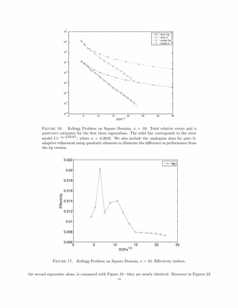
We compute eigenvalues on the analogous square domain (Figure 6), with a = 1 in M2 and a = κ =β2 = 10 in M1. The singular behavior of the eigenvectors near the cross point will be the same as for thecircular domain. In Figures 16-17 we report the total relative error and error estimates for the first threeeigenvalues, and the effectivity index. For these simulations we used the following reference values for thefirst three eigenvalues: 19.739208802 (1e-8), 30.264820 (1e-5), 70.310149038 (1e-8). Again we see apparentexponential convergence, with α = 0.2624.

5.6. Square Domain with a Slit. For this problem, L = −∆ and Ω = (0, 1)2 \ S, where S = (x, 1/2) :1/2 ≤ x ≤ 1; this is pictured in Figure 1, with S as the dashed segment. Homogeneous Neumann conditionsare imposed on both “sides” of S and homogeneous Dirichlet boundary conditions are imposed on the rest ofthe boundary of Ω. For this example we used the following reference values for the first four eigenvalues, withaccuracies given in parentheses: 20.739208802 (1e-8), 34.485320 (1e-5), 50.348022005 (1e-8), 67.581165196(1e-8).

To give some indication of the nature of the eigenvectors in the interior, we briefly consider a relatedproblem where Ω is the unit disk with a slit along the positive x-axis, as pictured in Figure 1, with the sameboundary conditions. In this case, the eigenvalues and eigenvectors are known explicitly. For k ≥ 0 andm ≥ 1, let zkm be the mth positive root of the first-kind Bessel function Jk/2. It is straightforward to verifythat, up to renormalization of eigenvectors, the eigenpairs can be indexed by

λkm = z2km , ψkm = Jk/2(zkmr) cos(kθ/2) , k ≥ 0 , m ≥ 1 .

We see that ψkm ∼ cos(kθ/2)(zkmr

2

)k/2as r → 0, so singularities of type rk/2 occur infinitely many times in

the spectrum. The strongest of these singularities is of type r1/2, and it occurs in the eigenvector associatedwith the second eigenvalue, for example. The same asymptotic behavior of the eigenvectors near the cracktip is expected for the square and circular domains, and in Figure 18 we show a contour plot of the secondeigenvalue for the square domain.

In Figure 19 we plot the total relative errors and error estimates for the first four eigenvalues withα = 0.3314, and in Figure 20 the individual eigenvalue errors are shown. It is clear from the second of thesefigures that the second eigenvalue, which corresponds to the most singular eigenvector, clearly has the worstconvergence rate (as expected), and that this is what “spoils” the convergence of the cluster of the first foureigenvalues. This becomes even more apparent when Figure 21 (with α = 0.3121), which corresponds to

18

0 5 10 15 20 25 30 3510

−6

10−5

10−4

10−3

10−2

10−1

100

101

102

DOFs1/3

error−hp

error−h

a post−hp

a post−h

Figure 16. Kellogg Problem on Square Domain, κ = 10: Total relative errors and aposteriori estimates for the first three eigenvalues. The solid line corresponds to the error

model Ce−2α3√DOFs, where α = 0.2642. We also include the analogous data for pure h-

adaptive refinement using quadratic elements to illustrate the difference in performance fromthe hp version.

0 5 10 15 20 250.006

0.008

0.01

0.012

0.014

0.016

0.018

0.02

0.022

DOFs1/3

Effectivity

hp

Figure 17. Kellogg Problem on Square Domain, κ = 10: Effectivity indices.

the second eigenvalue alone, is compared with Figure 19—they are nearly identical. Moreover in Figures 2219

Figure 18. Square Domain with Neumann-Neumann Slit: Contour plot of second eigenvector.

2 4 6 8 10 12 14 16 1810

−5

10−4

10−3

10−2

10−1

100

101

102

DOFs1/3

error

a post

Figure 19. Square Domain with Neumann-Neumann Slit: Total relative errors and aposteriori estimates for first four eigenvalues. The solid line corresponds to the error model

Ce−2α3√DOFs, where α = 0.3314.

20

2 4 6 8 10 12 14 16 1810

−10

10−8

10−6

10−4

10−2

100

DOFs1/3

err

or

eig 1

eig 2

eig 3

eig 4

Figure 20. Square Domain with Neumann-Neumann Slit: Relative errors for each of thefirst four eigenvalues individually.

2 4 6 8 10 12 14 16 1810

−5

10−4

10−3

10−2

10−1

100

101

DOFs1/3

error

a post

Figure 21. Square Domain with Neumann-Neumann Slit: Relative errors and a posterioriestimates for the second eigenvalue only. The solid line corresponds to the error model

Ce−2α3√DOFs, where α = 0.121.

and 23 we report the final mesh and the final distribution of polynomials orders for the second eigenvalue.As can be seen, the adaptive procedure has automatically heavily refined in the center, where the singularityis located.

21

Figure 22. Square Domain with Neumann-Neumann Slit: Final mesh and order of poly-nomials for the second eigenvalue only.

Acknowledgements

The work of L. Grubisic was supported by the grant: “Spectral decompositions – numerical methods andapplications”, Grant Nr. 037-0372783-2750 of the Croatian MZOS. The authors thank anonymous reviewersfor their valuable comments which improved the presentation of the paper.

References

[1] H. Ammari, Y. Capdeboscq, H. Kang, and A. Kozhemyak, Mathematical models and reconstruction methods in

magneto-acoustic imaging, European J. Appl. Math., 20 (2009), pp. 303–317.[2] H. Ammari, H. Kang, E. Kim, and H. Lee, Vibration testing for anomaly detection, Math. Methods Appl. Sci., 32 (2009),

pp. 863–874.

[3] H. Ammari, H. Kang, and H. Lee, Asymptotic analysis of high-contrast phononic crystals and a criterion for the band-gapopening, Arch. Ration. Mech. Anal., 193 (2009), pp. 679–714.

[4] M. G. Armentano, C. Padra, R. Rodrıguez, and M. Scheble, An hp finite element adaptive scheme to solve the

Laplace model for fluid-solid vibrations, Comput. Methods Appl. Mech. Engrg., 200 (2011), pp. 178–188.[5] M. Azaıez, M. O. Deville, R. Gruber, E. H. Mund, A new hp method for the −grad(div) operator in non-Cartesian

geometries, Appl. Numer. Math., 58 (2008), pp. 985–998.[6] I. Babuska and B. Q. Guo, The h-p version of the finite element method for domains with curved boundaries, SIAM

Journal on Numerical Analysis, 25 (1988), pp. 837–861.

[7] R. Bank, L. Grubisic, and J. S. Ovall, A framework for robust eigenvalue and eigenvector error estimation and ritzvalue convergence enhancement, Applied Numerical Mathematics, Volume 66 (2013), pp. 1–29.

[8] A. H. Barnett and T. Betcke, Stability and convergence of the method of fundamental solutions for Helmholtz problems

on analytic domains, J. Comput. Phys., 227 (2008), pp. 7003–7026.[9] T. Betcke, A GSVD formulation of a domain decomposition method for planar eigenvalue problems, IMA J. Numer.

Anal., 27 (2007), pp. 451–478.

22

Figure 23. Square Domain with Neumann-Neumann Slit: Final mesh and order of poly-nomials for the second eigenvalue only, showing a close-up of the central portion of thedomain (near the singularity).

[10] T. Betcke and L. N. Trefethen, Reviving the method of particular solutions, SIAM Rev., 47 (2005), pp. 469–491(electronic).

[11] M. Blumenfeld, Interface-Eigenwertprobleme auf polaren Gittern, Z. Angew. Math. Mech., 64 (1984), pp. 266–268.[12] , The regularity of interface-problems on corner-regions, in Singularities and constructive methods for their treatment

(Oberwolfach, 1983), vol. 1121 of Lecture Notes in Math., Springer, Berlin, 1985, pp. 38–54.[13] D. Boffi, F inite element approximation of eigenvalue problems, Acta Numer. 19 (2010), 1120.[14] T. Eibner and J. Melenk, An adaptive strategy for hp-FEM based on testing for analyticity, Comp. Mech., 39 (2007),

pp. 575–595.

[15] S. C. Eisenstat, On the rate of convergence of the Bergman-Vekua method for the numerical solution of elliptic boundaryvalue problems, SIAM J. Numer. Anal., 11 (1974), pp. 654–680.

[16] S. Giani and I. G. Graham, Adaptive finite element methods for computing band gaps in photonic crystals, Numer. Math.,(2011).

[17] S. Giani, L. Grubisic, and J. S. Ovall, Benchmark results for testing adaptive finite element eigenvalue procedures,

Appl. Numer. Math., Volume 62, Issue 2 (2012),pp. 121–140.[18] L. Grubisic, On eigenvalue and eigenvector estimates for nonnegative definite operators, SIAM J. Matrix Anal. Appl., 28

(2006), pp. 1097–1125 (electronic).

[19] L. Grubisic and K. Veselic, On weakly formulated Sylvester equations and applications, Integral Equations OperatorTheory, 58 (2007), pp. 175–204.

[20] L. Grubisic and J. S. Ovall, On estimators for eigenvalue/eigenvector approximations, Math. Comp., 78 (2009), pp. 739–

770.[21] P. Houston and E. Suli. A note on the design of hp-adaptive finite element methods for elliptic partial differential equations.

Comp. Methods in Appl. Mech. Eng., 194(2-5):229–243, Feb. 2005.

[22] R. B. Kellogg, On the Poisson equation with intersecting interfaces, Applicable Anal., 4 (1974/75), pp. 101–129.[23] A. Knyazev and O. Widlund, Lavrentiev regularization + Ritz approximation = uniform finite element error estimates

for differential equations with rough coefficients, Math. Comp., 72 (2003), pp. 17–40.

23

[24] P. D. Ledger, K. Morgan, The application of the hp-finite element method to electromagnetic problems, Arch. Comput.Methods Engrg., 12 (2005), pp. 235–302.

[25] B. J. McCartin, Eigenstructure of the equilateral triangle, part i: The dirichlet problem, SIAM Review, 45 (2003), pp. pp.

267–287.[26] J. M. Melenk and B. I. Wohlmuth, On residual-based a posteriori error estimation in hp-FEM, Adv. Comput. Math.,

15 (2001), pp. 311–331 (2002).

[27] P. Morin, R. H. Nochetto, and K. G. Siebert, Data oscillation and convergence of adaptive FEM, SIAM J. Numer.Anal., 38 (2000), pp. 466–488.

[28] S. Sauter, hp-finite elements for elliptic eigenvalue problems: error estimates which are explicit with respect to λ, h, andp, SIAM J. Numer. Anal., 48 (2010), 95108.

[29] B. Simon, Trace ideals and their applications, vol. 35 of London Mathematical Society Lecture Note Series, Cambridge

University Press, Cambridge, 1979.[30] R. Tankelevich, G. Fairweather, and A. Karageorghis, Three-dimensional image reconstruction using the PF/MFS

technique, Eng. Anal. Bound. Elem., 33 (2009), pp. 1403–1410.

Durham University, School of Engineering and Computing Sciences, South Road, Durham DH1 3LE, United

KingdomE-mail address: stefano.giani@durham.ac.uk

University of Zagreb, Department of Mathematics, Bijenicka 30, 10000 Zagreb, CroatiaE-mail address: luka.grubisic@math.hr

Portland State University 315 Neuberger Hall Portland, OR 97201, USAE-mail address: jovall@pdx.edu

24