Bernard MettlerThe Robotics Institute

Carnegie Mellon UniversityPittsburgh, PA

Takeo KanadeThe Robotics Institute

Carnegie Mellon UniversityPittsburgh. PA

Mark B. TischlerAeroftightdynamics Directorate (AMRDEC)

US Army Aviation and Missile CommandAmes Research Center, CA

This paper describes the development of a parameterized model for a small-scale unmanned helicopter (Yamaha R-50 with10 ft rotor diameter) and its identification using a frequency domain identification technique. The model explicitly accountsfor the stabilizer bar, which has a strong influence on the flight dynamics characteristics. The accuracy of the identified modelis verified by comparing the model-predicted responses with the responses collected during flight experiments. Furthermore,the values of key identified parameters are compared with the values predicted by helicopter theory to show that the modelhas a physically meaningful parameterization. Both hover and cruise flight conditions are examined.

Nomenclature

0, b longitudinal and lateral rotor flapping anglesc, d longitudinal and lateral stabilizer bar flapping anglesKd stabilizer bar gearingN scale factor; helicopter with 1/ N -th rotor diameterp, q, r roll, pitch, and yaw rates in helicopter reference frameu, v, w longitudinal, lateral, and vertical speed in helicopter

reference frame8col collective control input8/at cyclic lateral control input8/on cyclic longitudinal control input8 ped directional control inputy blade Lock numberYeff effective Lock numberYyu coherence function between system input u and output yr f main rotor time constantr, stabilizer bar time constant

Introduction

Small-scale helicopters are increasingly popular platforms for un-manned aerial vehicles (UAVs). The ability of helicopters to take off andland vertically, to perform hover flight as well as cruise flight, and theiragility, makes them ideal vehicles for a range of applications in a varietyof environments. Existing small-scale rotorcraft-based UAVs (RUAVs),however, exploit only a modest part of the helicopter's inherent qualities.For example, their operation is generally limited to hover and slow-speedflight, and their control performance is, in most cases, sluggish. Theselimitations on RUAV operation are mainly due to flight control systemsthat are designed without precise knowledge of the vehicle dynamics.

Throughout the 1990s, most RUAVs used classical control systemssuch as single-input-single-output proportional-derivative (PD) feedback

control systems. Their controller parameters were usually tuned empiri-cally. For more advanced multivariable controller synthesis approaches,an accurate model of the dynamics is recquired. Such models, however,are not readily available and are difficult to develop.

The dynamic models used for controller synthesis or controller op-timization have strict requirements. The model must capture the effectsthat govern the performance and maneuverability of the vehicle. High-bandwidth multivariable control requires models with high-bandwidthaccuracy. For helicopters, this implies that such a model must explicitlyaccount for effects such as the rotor-fuselage coupling. At the same time,however, the model must be simple enough to be insightful and practicalfor the controller synthesis.

Using a standard modeling approach based on first principles, consid-erable knowledge ofiotorcraft flight dynamics is required, and compre-hensive flight validations and model refinements are necessary to attainsufficient accuracy. System identification represents an attractive alter-native and has already been used successfully for full-scale helicopters(Refs. 1,2).

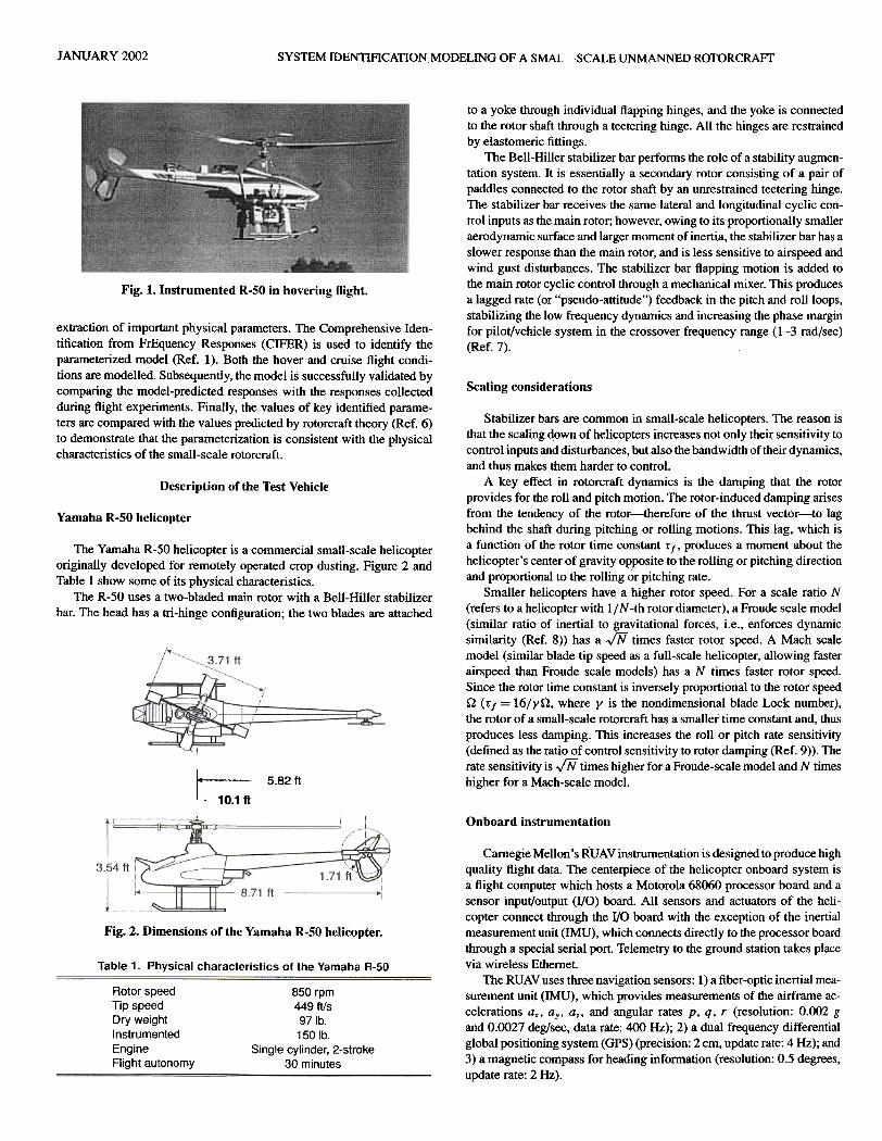
A few examples of the application of system identification techniquesto the modeling of small-scale helicopters exist. The results obtained arelimited compared with what is regularly achieved with full-scale heli-copters. For example, as shown in Ref. 3, to support model-based controldesign, the authors identified the rigid-body angular dynamics of the ve-hicle using measurements collected from a rigged helicopter. In anotherexample (Ref. 4), the authors developed a simulation model to evaluatevarious control strategies. They identified the vertical-longitudinal air-craft dynamics, with second-order pitch angle dynamics, from flight datacollected on a free-flying helicopter.. This paper describes the first comprehensive application of systemidentification techniques to a small-scale helicopter. Carnegie Mellon'sautonomous Yamaha R-50 helicopter (Ref. 5), shown in Fig. I, is usedto conduct the experiments. A complete parameterized model describingthe dynamics of the vehicle about its six degrees of freedom is devel-oped. The model includes the rotor and stabilizer bar dynamics, whichallow for improved high-bandwidth fidelity and, at the same time, for the~Manuscript received February 2000; accepted October 2001

50

JANUARY 2002 SYSTEM IDENTIFICATION MODELING OF A SMAL -SCALE UNMANNED ROTORCRAFf

to a yoke through individual flapping hinges, and the yoke is connectedto the rotor shaft through a teetering hinge. All the hinges are restrainedby elastomeric fittings.

The Bell-Hiller stabilizer bar performs the role of a stability augmen-tation system. It is essentially a secondary rotor consisting of a pair ofpaddles connected to the rotor shaft by an unrestrained teetering hinge.The stabilizer bar receives the same lateral and longitudinal cyclic con-trol inputs as the main rotor; however, owing to its proportionally smalleraerodynamic surface and larger moment of inertia, the stabilizer bar has aslower response than the main rotor, and is less sensitive to airspeed andwind gust disturbances. The stabilizer bar flapping motion is added tothe main rotor cyclic control through a mechanical mixer. This producesa lagged rate (or "pseudo-attitude") feedback in the pitch and roll loops,stabilizing the low frequency dynamics and increasing the phase marginfor pilot/vehicle system in the crossover frequency range (1-3 rad/sec)(Ref. 7).

Fig. 1. Instrumented R-50 in hovering flight.

extraction of important physical parameters. The Comprehensive Iden-tification from FrEquency Responses (CIFER) is used to identify theparameterized model (Ref. 1). Both the hover and cruise flight condi-tions are modelled. Subsequently, the model is successfully validated bycomparing the model-predicted responses with the responses collectedduring flight experiments. Finally, the values of key identified parame-ters are compared with the values predicted by rotorcraft theory (Ref. 6)to demonstrate that the parameterization is consistent with the physicalcharacteristics of the small-scale rotorcraft.

Scaling considerations

Description of the Test Vehicle

Yamaha R-SO helicopter

Stabilizer bars are common in small-scale helicopters. The reason isthat the scaling ~own of helicopters increases not only theil: sensitivity tocontrol inputs and disturbances, but also the bandwidth of their dynamics,and thus makes them harder to control.

A key effect in rotorcra,ft dynamics is the damping that the rotorprovides for the roll and pitch motion. The rotor-induced damping arisesfrom the tendency of the rotor-therefore of the thrust vector-to lagbehind the shaft during pitching or rolling motions. This lag, which isa function of the rotor time constant T I, produces a moment about thehelicopter's center of gravity opposite to the rolling or pitching directionand proportional to the rolling or pitching rate.

Smaller helicopters have a higher rotor speed. For a scale ratio N(refers to a helicopter with II N -th rotor diameter), a Froude scale model(similar ratio of inertial to gravitational forces, i.e., enforces dynamicsimilarity (Ref. 8» has a J"N" times faster rotor speed. A Mach scalemodel (similar blade tip speed as a full-scale helicopter, allowing fasterairspeed than Froude scale models) has a N times faster rotor speed.Since the rotor time constant is inversely proportional to the rotor speedQ (TI = 161yQ, where y is the nondimensional blade Lock number),

the rotor of a small-scale rotorcraft has a smaller time constant and, thusproduces less damping. This increases the roll or pitch rate sensitivity(defined as the ratio of control sensitivity to rotor damping (Ref. 9». Therate sensitivity is J"N" times higher for a Froude-scale model and N timeshigher for a Mach-scale model.

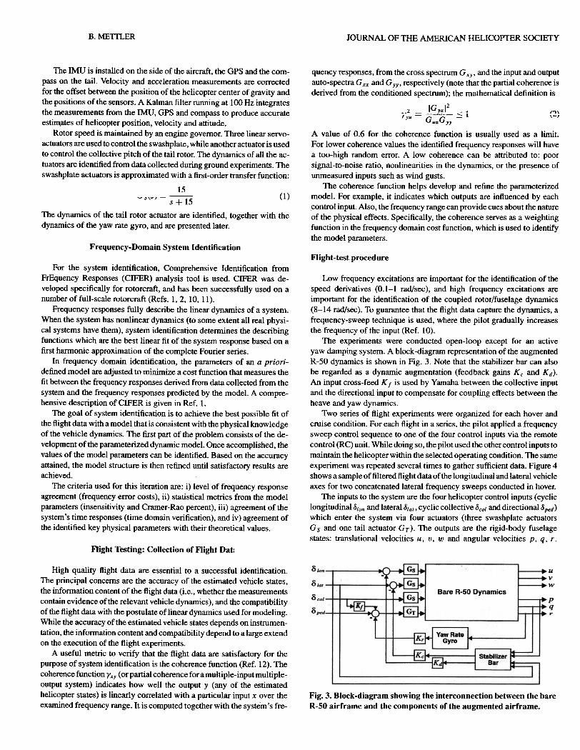
The Yamaha R-50 helicopter is a commercial small-scale helicopteroriginally developed for remotely operated crop dusting. Figure 2 andTable I show some of its physical characteristics.

The R-50 uses a two-bladed main rotor with a Bell-Hiller stabilizerbar. The head has a tri-hinge configuration; the two blades are attached

~ 5.82 ft

Onboard instrumentation

Fig. 2. Dimensions of the Yamaha R-50 helicopter.

Table 1. Physical characteristics of the Yamaha A-50

Carnegie Mellon's RUA V instrumentation is designed to produce highquality flight data. The centerpiece of the helicopter onboard system isa flight computer which hosts a Motorola 68060 processor board and asensor input/output (I/O) board. All sensors and actuators of the heli-copter connect through the I/O board with the exception of the inertialmeasurement unit (IMU), which connects directly to the processor boardthrough a special serial port. Telemetry to the ground station takes placevia wireless Ethernet.

The RUAV uses three navigation sensors: I) a fiber-optic inertial mea-surement unit (IMU), which provides measurements of the airframe ac-celerations ax, ay, az, and angular rates p, q, r (resolution: 0.002 gand 0.0027 deg/sec, data rate: 400 Hz); 2) a dual frequency differentialglobal positioning system (GPS) (precision: 2 cm, update rate: 4 Hz); and3) a magnetic compass for heading information (resolution: 0.5 degrees,update rate: 2 Hz).

Rotor speedTip speedDry weightInstrumentedEngineFlight autonomy

850 rpm449 fils97 lb.150 lb.

Single cylinder, 2-stroke30 minutes

B. MElTLER JOURNAL OF THE AMERICAN HELICOPTER SOCIETY

quency responses, from the cross spectrum G xy' and the input and outputauto-spectra G xx and G yy' respectively (note that the partial coherence isderived from the conditioned spectrum); the mathematical definition is

v2 = IGyuf -. (?)

The IMU is installed on the side of the aircraft, the GPS and the com-pass on the tail. Velocity and acceleration measurements are correctedfor the offset between the position of the helicopter center of gravity andthe positions of the sensors. A Kalman filter running at 100 Hz integratesthe measurements from the IMU, GPS and compass to produce accurateestimates of helicopter position, velocity and attitude.

Rotor speed is maintained by an engine governor. Three linear servo-actuators are used to control the swashplate, while another actuator is usedto control the collective pitch of the tail rotor. The dynamics of all the ac-tuators are identified from data collected during ground experiments. Theswashplate actuators is approximated with a first-order transfer function:

15r..(~) =

fyu -G G ::: 1 ,-/UU yy

A value of 0.6 for the coherence function is usually used as a limit.For lower coherence values the identified frequency responses will havea too-high random error. A low coherence can be attributed to; poorsignal-to-noise ratio, nonlinearities in the dynamics, or the presence ofunmeasured inputs such as wind gusts.

The coherence function helps develop and refine the parameterizedmodel. For example, it indicates which outputs are influenced by eachcontrol input. Also, the frequency range can provide cues about the natureof the physical effects. Specifically, the coherence serves as a weightingfunction in the frequency domain cost function, which is used to identifythe model parameters.

-",-, ;+l5 (1)

The dynamics of the tail rotor actuator are identified, together with thedynamics of the yaw rate gyro, and are presented later.

Frequency-Domain System IdentificationFlight-test procedure

Low frequency excitations are important for the identification of thespeed derivatives (0.1-1 rad/sec), and high frequency excitations areimportant for the identification of the coupled rotor/fuselage dynamics(8-14 rad/sec). To guarantee that the flight data capture the dynamics, afrequency-sweep technique is used, where the pilot gradually increasesthe frequency of the input (Ref. 10).

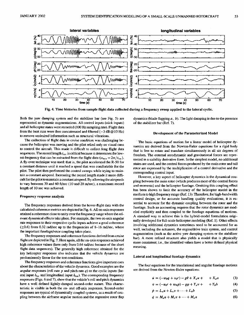
The experiments were conducted open-loop except for an activeyaw damping system. A block-diagram representation of the augmentedR-50 dynamics is shown in Fig. 3. Note that the stabilizer bar can alsobe regarded as a dynamic augmentation (feedback gains Kc and Kd).An input cross-feed K f is used by Yamaha between the collective inputand the directional input to compensate for coupling effects between theheave and yaw dynamics.

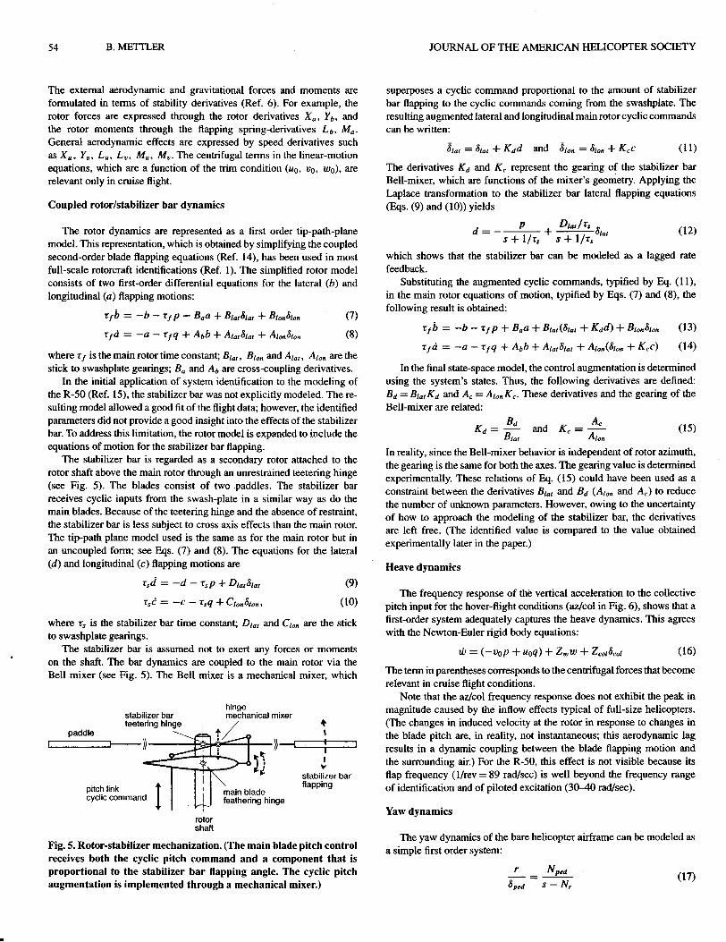
Two series of flight experiments were organized for each hover andcruise condition. For each flight in a series, the pilot applied a frequencysweep control sequence to one of the four control inputs via the remotecontrol (RC) unit. While doing so, the pilot used the other control inputs tomaintain the helicopter within the selected operating condition. The sameexperiment was repeated several times to gather sufficient data. Figure 4shows a sample of filtered flight data of the longitudinal and lateral vehicleaxes for two concatenated lateral frequency sweeps conducted in hover.

The inputs to the system are the four helicopter control inputs (cyclic10ngitudinalcS1on and lateralcS1at, cyclic collective cScoI and directionalcSped)which enter the system via four actuators (three swashplate actuatorsG s and one tail actuator GT ). The outputs are the rigid-body fuselagestates: translational velocities u, v, w and angular velocities p, q, r.

For the system identification, Comprehensive Identification fromFrEquency Responses (CIFER) analysis tool is used. CIFER was de-veloped specifically for rotorcraft, and has been successfully used on anumber of full-scale rotorcraft (Refs. 1,2, 10, II).

Frequency responses fully describe the linear dynamics of a system.When the system has nonlinear dynamics (to some extent all real physi-cal systems have them), system identification determines the describingfunctions which are the best linear fit of the system response based on afirst harmonic approximation of the complete Fourier series.

In frequency domain identification, the parameters of an a priori-defined model are adjusted to minimize a cost function that measures thefit between the frequency responses derived from data collected from thesystem and the frequency responses predicted by the model. A compre-hensive description of CIFER is given in Ref. I.

The goal of system identification is to achieve the best possible fit ofthe flight data with a model that is consistent with the physical knowledgeof the vehicle dynamics. The first part of the problem consists of the de-velopment of the parameterized dynamic model. Once accomplished, thevalues of the model parameters can be identified. Based on the accuracyattained, the model structure is then refined until satisfactory results areachieved.

The criteria used for this iteration are: i) level of frequency responseagreement (frequency error costs), ii) statistical metrics from the modelparameters (insensitivity and Crarner-Rao percent), iii) agreement of thesystem's time responses (time domain verification), and iv) agreement ofthe identified key physical parameters with their theoretical values.

Flight Testing: Collection of Flight Dat:

High quality flight data are essential to a successful identification.The principal concerns are the accuracy of the estimated vehicle states,the infonnation content of the flight data (i.e., whether the measurementscontain evidence of the relevant vehicle dynamics), and the compatibilityof the flight data with the postulate of linear dynamics used for modeling.While the accuracy of the estimated vehicle states depends on instrumen-tation, the infonnation content and compatibility depend to a large extendon the execution of the flight experiments.

A useful metric to verify that the flight data are satisfactory for thepurpose of system identification is the coherence function (Ref. 12). Thecoherence function Yxy (or partial coherence for a multiple-input multiple-output system) indicates how well the output y (any of the estimatedhelicopter states) is linearly correlated with a particular input x over theexamined frequency range. It is computed together with the system's fre-

Fig. 3. Block-diagram showing the interconnection between the bareR-SO airframe and the components of the augmented airframe.

JANUARY 2002 SYSTEM IDENnFICATION MODELING OF A SMALL-SCALE UNMANNED ROTORCRAFI 53

lateral variables longitudinal variables~ 40 ~~J\j\M~~,f"'Vv~Jv\/\f~~~'t~ 1 ~ 40

~ ~--~_.~-,\~~""---v~-..,,-~-"""\,.i~VJ~~~ - c

~-40 .Q -40

150 k:A J\ A/\lIhAAAA~~ ~ A /\ f\ 'AAAM~ 150 I=====:::::::::::;;::===~=====:=~Jo.-50~ - ,""'" ""',"v'Y'V'.llq -, ~.'1 \J~~II"'I".~ C"-50~' ,','. , , ,~

i20~ 1\ J\~AI\'AAAA'"..,.A.:-A {\ /\I\' ~ ~ i20r -="~' --'- '--'""'.~~

-a.-20r::- V, V ~V'Y""~ ~ V.. V v~vv"-'-,l :s-20r:::::::~==:::=====::~~ ~ ,1

i 4~ !\ 1\ ~AAJ\AMA~I'..,.-"\ ~ f'\ /\ A"AAAl'I~j i 4~' - ~. '--'~ : ~ :-J

.~ -4~ - V, ~ v,v'v"",!"" v:v. V v~VV"VWfr, l.~ -4f====, ~ -: ~ ~ , 1

-;;- 4~ r\i\j~-v--"""""-:'", ~--/\I\f\~YJ-~~ 1 ~ 4

~ .-~---~-"",--~/~~~ ~ \.-//~"'-_r1 E E

~-4 ~-410 20 30 40 50 60 70 10 20 30 40 50 60 70

time (s) time (s)

Fig. 4. Time histories from sample flight data collected during a frequency sweep applied to the lateral cyclic.

dynamics (blade flapping a, b). The light damping is due to the presenceof the stabilizer bar (Ref. 7).

Development of the Parameterized Model

Both the yaw damping system and the stabilizer bar (see Fig. 5) arerepresented as dynamic augmentations. All control inputs (stick inputs)and all helicopter states were recorded (I ()() Hz sampling rate). Flight datafrom the best runs were then concatenated and filtered (-3 dB@ 10 Hz)to remove undesired information such as structural vibrations.

The collection of flight data in cruise condition was challenging be-cause the helicopter was moving and the pilot relied only on visual cuesto control the aircraft. This made it difficult to collect long flight datasequences. The record length trec is critical because it determines the low-est frequency that can be extracted from the flight data (Wmin = 27f / trec)'

A fly-over technique was used: that is, the pilot accelerated the R-50 fora constant distance until it reached a speed that was comfortable for thepilot. The pilot then performed the control sweeps while trying to main-tain a constant airspeed. Increasing the record length made it morediffi-cult for the pilot to maintain a constant airspeed. By allowing the airspeedsto vary between 30 and 60 ft/sec (10 and 20 m/sec), a maximum recordlength of 10 sec was achieved.

The basic equations of motion for a linear model of helicopter dy-namics are derived from the Newton-Euler equations for a rigid bodythat is free to rotate and translate simultaneously in all six degrees offreedom. The external aerodynamic and gravitational forces are repre-sented in a stability derivative form. In the simplest model, no additionalstates are used, and the control forces produced by the main rotor and tailrotor are expressed by the multiplication of a control derivative and thecorresponding control input.

However, a key aspect of helicopter dynamics is the dynamical cou-pling between the main rotor (which produces most of the control forcesand moments) and the helicopter fuselage. Omitting this coupling effecthas been shown to limit the accuracy of the helicopter model in themedium to high frequency range (Ref. 13). Therefore, for high-bandwidthcontrol design, or for accurate handling quality evaluations, it is es-sential to account for the dynamic coupling between the rotor and thefuselage. Such an accounting requires that the rotor dynamics are mod-eled explicitly and then coupled to the fuselage equations of motions.A standard way to achieve this is the hybrid-model formulation origi-nally developed for full-scale helicopter modeling (Ref. I). Other effectsinvolving additional dynamics sometimes need to be accounted for aswell, including the actuators, the engine/drive train system, and controlaugmentation (such as the active yaw damping system or the stabilizerbar). A more refined structure also yields a model that is physicallymore consistent; i.e., the identified values have a better defined physicalmeaning;.

Frequency response analysis

Lateral and longitudinal fuselage dynamics

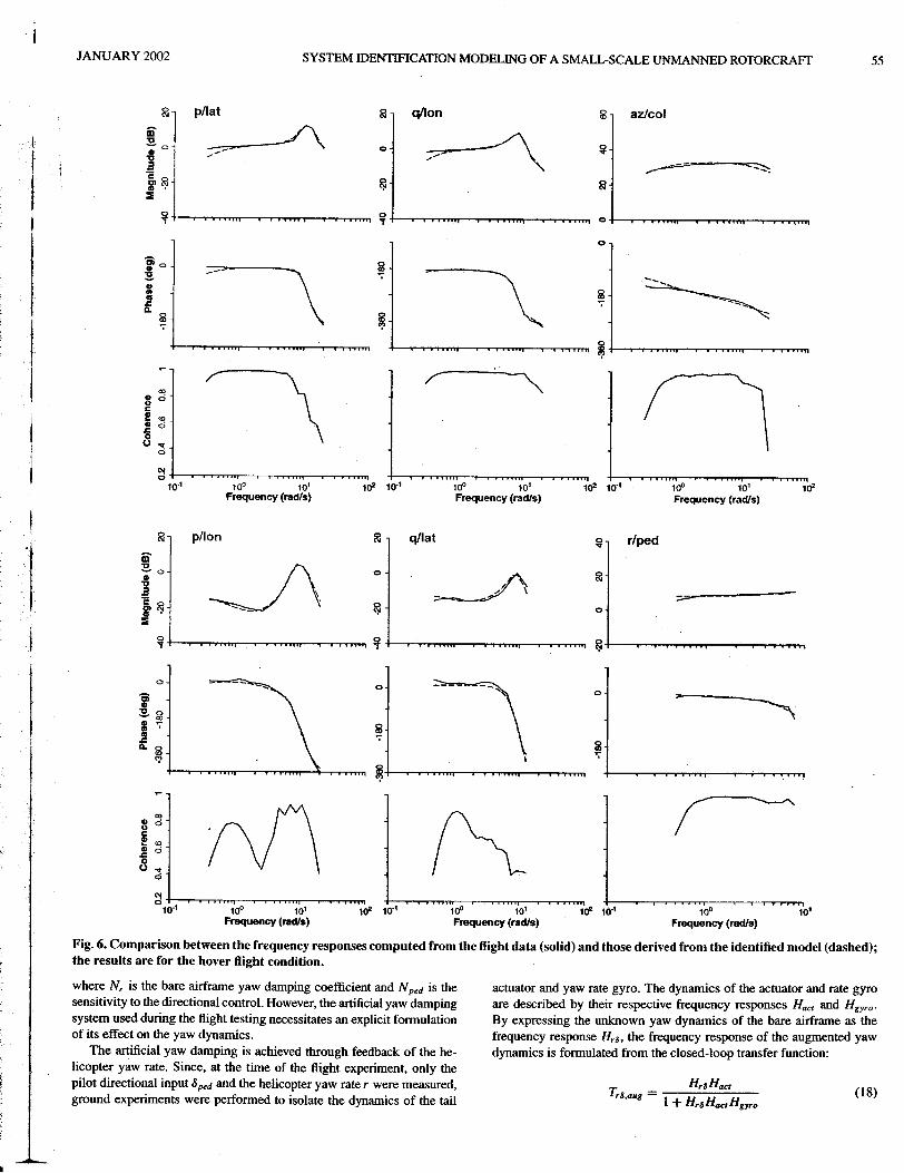
The frequency responses derived from the hover-flight data with thecalculated coherence metrics are depicted in Fig. 6. All on-axis responsesattained a coherence close to unity over the frequency range where the rel-evant dynamical effects take place. For example, the two on-axis angularrate responses to their respective cyclic inputs achieve a good coherence(?:0.6) from 0.32 rad/sec up to the frequencies of 8-16 rad/sec, wherethe important fuselage/rotor coupling takes place.

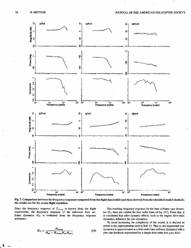
The frequency responses and coherence functions derived from cruiseflight are depicted in Fig. 7. Here again, all the on-axis responses achievedhigh coherence values (here only from 0.64 rad/sec because of the shortflight data sequences). The generally high coherence obtained for thekey helicopter responses also indicates that the vehicle dynamics arepredominantly linear for the test conditions.

The frequency responses and coherence functions give important cuesabout the characteristics of the vehicle dynamics. Good examples are theangular responses (roll rate p and pitch rate q) to the cyclic inputs (lat-eral input 81at and longitudinal input 810/1). The corresponding frequencyresponses (Figs. 6 and 7), show that the vehicle's roll and pitch dynamicshave a well defined lightly-damped second-order nature. This charac-teristic is visible in both the on- and off-axis responses. Second-orderresponses are typical of dynamically coupled systems, as a result of cou-pling between the airframe angular motion and the regressive rotor flap

The four equations for the translational and angular fuselage motionsare derived from the Newton-Euler equations:

+Xaa

+Ybb

(3)

(4)

(5)

(6)

It = (-woq + vor) - g() + Xuu +

Ii = (-uor + wop) - g<p + Yvv +

p = Luu+Lvv+...+Lbh

q = Mu~ + Mvv + ... + Maa

54 B. ME1TLER JOURNAL OF THE AMERICAN HELICOPTER SOCIETY

The external aerodynamic and gravitational forces and moments are superposes a cyclic command proportional to the amount of stabilizerformulated in terms of stability derivatives (Ref. 6). For example, the bar flapping to the cyclic commands coming from the swashplate. Therotor forces are expressed through the rotor derivatives Xa, Yb, and resulting augmented lateral and longitudinal main rotor cyclic co mmandsthe rotor moments through the flapping spring-derivatives Lb. Ma. can be written:General aerodynamic effects are expressed by speed derivatives such . -. + K d d . -. + K (11). .". Ulat - alar d an ulan - ulon cCas Xu,, Y v, Lu. Lv, Mu, Mv. The centnfugal terms m the lInear-motIon

equations, which are a function of the trim condition (uo, va, wo), are The derivatives Kd and Kc represent the gearing of the stabilizer barrelevant only in cruise flight. Bell-mixer, which are functions of the mixer's geometry. Applying the

Laplace transformation to the stabilizer bar lateral flapping equationsCoupled rotor/stabilizer bar dynamics (Eqs. (9) and (10» yields

. . P Dlat/l", 2The rotor dynamics are represented as a first order tIp-path-plane d = - + 8lot (1 )model. This representation, which is obtained by simplifying the coupled S + 1/1", S + 1/1",

second-order blade flapping equations (Ref. 14), has been used in most which shows that the stabilizer bar can be modeled as a lagged ratefull-scale rotorcraft identifications (Ref. I). The simplified rotor model feedback.consists of two first-order differential equations for the lateral (b) and Substituting the augmented cyclic commands, typified by Eq. (11),longitudinal (a) flapping motions: in the main rotor equations of motion, typified by Eqs. (7) and (8), the

b. - b B B . B . 7 following result is obtained:I"f - - - I"fP - oa + lotalat + lonalon ( )

'- +Ab A . A . (8) t"fb=-b-t"fp+Baa+Blat(8lat+Kdd)+Blon8lon (13)t"fa - -a - I"fq b + latUlat + 10nUIon. . . t"fa = -a - t"fq + Abb + Alat8lat + Alon(8lon + Kcc) (14)

where I" f IS the maIn rotor tIme constant; Blat, Blon and Alot, Alon are the

stick to swashplate gearings; Ba and Ab are cross-coupling derivatives. In the final state-space model, the control augmentation is determinedIn the initial application of system identification to the modeling of using the system's states. Thus, the following derivatives are defined:

the R-50 (Ref. 15), the stabilizer bar was not explicitly modeled. The re- Bd = BlatKd and Ac = AlonKc. These derivatives and the gearing of thesuiting model allowed a good fit of the flight data; however, the identified Bell-mixer are related:parameters did not provide a good insight into the effects of the stabilizer Bd Acbar. To address this limitation, the rotor model is expanded to include the Kd = ~ and Kc = ~ (15)

equations of motion for the stabilizer bar flapping. I I.t . th B II . beh . .. d d t f t .th. . n rea I y, sInce e e -mixer avlor IS m epen en 0 ro or azlmu ,

The stabilIZer bar is regarded as a secondary rotor attached to the th .. th " bothth Th . I " d t . de geanng IS e same lor e axes. e geanng va ue IS e ermInerotor shaft above the main rotor through an unrestrained teetering hinge . t II Th I t . f Eq (15) Id h be dexpenmen a y. ese re a Ions 0 . cou ave en use as a

(see Fig. 5). The blades consist of two paddles. The stabilizer bar t . t bet th d . tI. B d B (A d A ) t d. . . . .. cons ram ween e enva ves lat an d Ion an core ucereceives cyclic mputs from the swash-plate m a similar way as do the th be f nkn t H " t th rt . te num r 0 u own parame ers. owever, owmg 0 e unce am y

main blades. Because of the teetering hinge and the absence of restraint, f h t h th od I. f th tab.l . b th d . t.. . . 0 ow 0 approac e m e mg 0 e s I lzer ar, e enva Ives

the stabilizer bar IS less subject to cross axis effects than the main rotor. I ft f (Th .d t.fi d I . ed t th I btam.d.. are e ree. e I en I e va ue IS compar 0 e va ue 0 e

The tIp-path plane model used IS the same as for the main rotor but in . tall I t . th )expenmen y a er m e paper.an uncoupled form; see Eqs. (7) and (8). The equations for the lateral(d) and longitudinal (c) flapping motions are Heave dynamics

I",d = -d - 1", P + Dlat8lat (9). The frequency response of the vertical acceleration to the collective

t",C = -c - t",q + Clon8lon, (10) pitch input for the hover-flight conditions (az/col in Fig. 6), shows that a

where I" is the stabilizer bar time constant D and C are the stick first-order system adequately captures the heave dynamics. This agrees, , lat Ion . . . .

to swashplate gearings. with the Newton-Euler ngld body equatIons:

The stabilizer bar is assumed not to exert any forces or moments iii = (-vop + uoq) + Zww + Zco/8col (16). on the shaft. The bar dynamics are coupled to the main rotor via the. .Bell mixer (see Fig. 5). The Bell mixer is a mechanical mixer which The term m parentheses corresponds to the centnfugal forces that become

, relevant in cruise flight conditions.

Note that the az/col frequency response does not exhibit the peak intab ' l " b hinge h . I " magnitude caused by the inflow effects typical of full-size helicopters.

s Ilzer ar mec amca mixerteetering hinge / It (The changes in induced velocity at the rotor in response to changes in

paddle t / - I the blade pitch are, in reality, not instantaneous; this aerodynamic lagI I-- ~ ))-: I results in a dynamic coupling between the blade flapping motion and

I i ~ the surrounding air.) For the R-50, this effect is not visible because its~ stabilizer bar flap frequency (I/rev = 89 rad/sec) is well beyond the frequency range

pitc~ link I de flapping of identification and of piloted excitation (30--40 rad/sec).cyclic command ng hinge

I Yaw dynamicsrotorshaft

. . . . . .. The yaw dynamics of the bare helicopter airframe can be modeled asFig. 5. Rotor-stabilizer mechanIzation. (The mam blade pitch control a simple first order system:receives both the cyclic pitch command and a component that isproportional to the stabilizer bar flapping angle. The cyclic pitch ~ = ~ (17)augmentation is implemented through a mechanical mixer.) 8ped S - Nr

.

.jJANUARY 2002 SYSTEM IDENTIFICATION MODELING OF A SMALL-SCALE UNMANNED ROTORCRAFf 55

@ pIlat ~ q/lon ~ az/col

~ 0 ?= ~/\ 0::::;~---"'/-\, ~'U - ...

; ~ ..-==-' ---~: -g,@ ~ ~c ' .~

0 0 0.,. .,.

0

i 0 ::-::~ \ a! \fa! - \: ~ ~ :.:::.:::_--~="..",.",~

';- .~

'I .

J g~ ~ /---~ II' ! <0I' e ci.c0<J ...

ci

j "I

010" 10° 10' 10' 10-' 10° 10' 10' 10" 100 10' 10'Frequency (rad's) Frequency (rad/s) Frequency (rad/s)

.I: ~ pIlon ~ q/lat ~ r/ped

m'U -."",.~ --0 0 0 j II, ;:: ?~!~ '" =- --

s.@ -- @ 0! C . .~

I 0 Q ~.,. .,. .

fO - 0 \- - -- 0 ~ ~--a!e ~ 0e . '"c ~.c . 2

Q. 0 ~<0 \ .c:> ~

g ~r\r\ ~ (" '"

! <0e '.c 0

0<J...

ci

"I010" 10° 10' 10' 10" 100 10' 10' 10" 10° 10'

Frequency (rad/s) Frequency (rad/s) Frequency (radls)

Fig. 6. Comparison between the frequency responses computed from the flight data (solid) and those derived from the identified model (dashed);the results are for the hover flight condition.

where N r is the bare airframe yaw damping coefficient and N ped is the actuator and yaw rate gyro. The dynamics of the actuator and rate gyrosensitivity to the directional control. However, the artificial yaw damping are described by their respective frequency responses Hac! and H gyra'system used during the flight testing necessitates an explicit formulation By expressing the unknown yaw dynamics of the bare airframe as theof its effect on the yaw dynamics. frequency response Hr6, the frequency response of the augmented yaw

The artificial yaw damping is achieved through feedback of the he- dynamics is formulated from the closed-loop transfer function:licopter yaw rate. Since, at the time of the flight experiment, only thepilot directional input Oped and the helicopter yaw rate r were measured, 7: = Hr&Hac! (18)ground experiments were performed to isolate the dynamics of the tail r6,a..g 1 + Hr6HacrHgyro

!

56 B. MElTLER JOURNAL OF THE AMERICAN HELICOIYrER SOCIETY

@ p/lat @ q/lon ~ az/col

i -=-./\ - --,-0 0 0. ..'C ===~~ --~ -e010 @ 0. ')' . C\j

~

~ ~ 0

0

I : \ : \ ~ ""' ~~

~i : \ ---'""-""\ ~u.. \

ci

C\jci

10-' 10° 10' 100 10-' 100 10' 100 10-' 10° 10' 100Frequency (rad/s) Frequency (rad/s) Frequency (rad/s)

@ p/lon @ q/lat ~ r/ped

m'C-0 0 @! ~ - - - .,.,." = ~ =e 0 0 001", C\j. . .~

~ ~ ~

~ ~ ====""'-:::~- -01 ---3 0 -~ = =, , 0 =~-~~-~:::~~,,- - - - - 0 - - -- -- , ,...m~II.

2 ~ 2~ ~ ~. , .

i : --~/-V ( "",,~ I-/-/-"---~.c 00u..

ci

C\jci

10-' 10° 10' 100 10' 100 10'Frequency (rad/e) Frequency (rad/s) Frequency (rad/e)

Fig. 7. Comparison between the frequency responses computed from the ftight data (solid) and those derived from the identified model (dashed);the results are for the cruise ftight condition.

Since the frequency response of T r8.aug is known from the flight The resulting frequency response for the bare airframe yaw dynam-experiments, the frequency response of the unknown bare air- ics Hr8 does not exhibit the first order form of Eq. (17). From this, itframe dynamics Hr8 is evaluated from the frequency response is concluded that other dynamic effects, such as the engine drive-trainarithmetic: dynamics, influence the yaw dynamics.

To avoid increasing the complexity of the model, it is decided torevert to the representation used in Ref. 15. That is, the augmented yaw

Hr8 = Hr8.aug (19) dynamics is approximated as a first-order bare airframe dynamics with aHact - Hr8.augHactHgyro yaw rate feedback represented by a simple first-order low-pass filter:

l-""-'--I

!

I

.. JANUARY 2002 SYSTEM illENTIFICATION MODELING OF A SMALL-SCALE UNMANNED ROTORCRAFT 57jJ.r

Ii Xu 0: 0 0:0 -g Xa 0 0 0 0: 0 0 u 0 0 I 0 0I I I I

-~- 0 y,,! 0 0: gOO Yb 0 0 0: 0 0 v 0 o! YfMd 0I . ' T ~ -- , p ~ 4:00:000 £,,£,;. 00:00 p 00; 0 0

I I I 1

q M" M,,: 0 0: 0 0 Ma 0 Mw 0 0: 0 0 q 0 0: 0 Mcol--- ~ ~ ~-- ~;p 0 0: 1 0: 0 0 0 0 0 0 0: 0---0 -i -0 0- :--0 0-

1 I I 1 [ 8 ]iJ 0 0: 0 1:0 0 0 0 0 0 0: 0 0 8 0 0: 0 0 Iat- I I I - I 8'rIa = 0 0: 0 -1"1: 0 0 -I ~ 0 0 0: Ac 0 a + ~ ~! 0 0 Ion

. I I I I 8fMd'rIb 0 0: -1"1 0: 0 0 Ba -I 0 0 0: 0 Bd b Blat BIon: 0 0~ 0 0: 0 0: 0 0 Za ~ Zw Z, 0: 0 0 -; 0 0: 0 ~I 8col-~- ~ + ~ -- J f 0 N" I Np 0 10 0 0 0 Nw N, N I 0 0 rOO: N N

colI. I "JV I I YO"I I 1 I

rj/J 0 0: 0 0: 0 0 0 0 0 K, KIj#1: 0 0 rj/J 0 0: 0 0--- ~ ~ ~ -- ~ 'rsi: 0 0: 0 -1"8: 0 0 0 0 0 0 0: -I 0 c 0 Cion: 0 0

I I I I. " I'r8d 0 o! -1"8 O! 0 0 0 0 0 0 O! 0 -I d DIal 0: 0 0

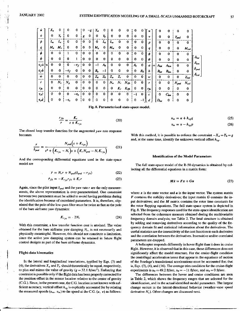
Fig. 8. Parameterized state-space model.

~ = ~ (20) Um = U + hcgq (25)r s + K'fb Vm = v - hcgp (26)

The closed loop transfer function for the augmented yaw rate responsebecomes With this method, it is possible to enforce the constraint - Xa = Y b = g

( ) and, at the same time, identify the unknown vertical offset hcg.r Nped S + K'fb

- = (21)8ped S2 + (K'fb - N,)s + (K,Nped - N,K'fb)

Identification of the Model ParametersAnd the corresponding differential equations used in the state-spacemodel are The full state-space model of the R-50 dynamics is obtained by col-

lecting all the differential equations in a matrix form:r = N,r + N ped«(,ped - rIb) (22)

rIb = -K'fbrfb + K,r (23) Mot = Fx + Gu (27)

Again, since the pilot input (,ped and the yaw rate r are the only measure-ments, the above representation is over-parameterized. One constraint where x is the state vector and u is the input vector. The system matrixbetween two parameters must be added to avoid having problems during F contains the stability derivatives; the input matrix G contains the in-the identification because of correlated parameters. It is, therefore, stip- put derivatives; and the M matrix contains the rotor time constants forulated that the pole of the low-pass filter must be twice as fast as the pole the rotor flapping equations. The full state-space system is depicted inof the bare airframe yaw dynamics: Fig. 8. The frequency responses used for the state-space identificatiQn are

selected from the coherence measure obtained during the multivariableK'fb = -2N, (24) frequency domain analysis; see Table 2. The final structure is obtained

... .. . by adding and removing derivatives according to the quality of the fre-With this constraint, a low transfer function cost IS attained. The value d . fi d .. al . " . bo th d . .

Th. . .. . quency omaln t an StatIStiC InlOrmatIon a ut e envatlves. eobtained for the bare airframe yaw damping N" IS not necessarily and . . .. . . . . .

h . 11 . ti 1 H h. h Id . 1... useful statIstIcs are the insensItIvity of the cost functIon to each denvatIvep yslca y meamng u. owever, t IS S ou not constItute a ImitatIon, . ... .. th . dam . be . d . ti fl . h and the correlatIon between the denvatIves. InsensItIve and/or correlated

since e actIve yaw ping system can retalne In uture Ig td dI d . f h b .rf . parameters are roppe .

contro eslgns as part 0 t e are aI rame dynamics. A h I. d d."" I . h fl . h h . d . .e Icopter respon s Illerent y In over Ig t t an It oes In cruIse

flight. However, it is observed that in this case, these differences does notI Flight-data kinematics significantly affect the model structure. For the cruise-flight condition

the centrifugal acceleration terms that appear in the equations of motion,. In the lateral and longitudinal translations, typified by Eqs. (3) and of the fuselage's translational accelerations must be accounted for; thati (4), the derivatives Xa and Y b should theoretically be equal, respectively, is, Eqs. (3), (4), and (16). The average trim condition for the cruise-flight

to plus and minus the value of gravity (g = 32.1 ftlsec2). Enforcing that experiments is Uo = 49.2 ft/sec, Vo = -II ft/sec, and Wo = 0 ft/sec.! constraint is possible only if the flight data has been properly corrected for The differences between the hover and cruise conditions are seen

the position offset in the sensor location relative to the center of gravity in Table 2, which shows the frequency ranges that are selected for the(C.G.). Since, in the present case, the C.G.location is not known with suf- identification, and in the actual identified model parameters. The largest

! ficient accuracy, vertical offset hcg is explicitly accounted for by relating change occurs in the lateral-directional behavior (weather-vane speedthe measured speeds (um, vm) to the speed at the C.G. (u, v) as follows: derivative Nv). Other changes are discussed next.

:.,..;, !

58 B. METI1..ER JOURNAL OF THE AMERICAN HELICOPTER SOCIETY

Table 2. Frequency responses and frequency ranges selected for Table 3. Transfer function costs attained for each input-output pairthe identification process. (First row: hover condition; second row: during the identification

cruise flight condition). Notice that not all input-output pairsare used Hover Cruise

vx/lat 15.7b'at blan bcol bped vy/lat 18.4

p 0.32-20 0.4-20 - vz/lat 71..10.7-20 0.7-14 2.4-16 - p/lat 61.5 13

q 0.4-20 0.32-20 q/lat 50.4 18.51.6-10 0.7-20 0.7-18 ax/lat 15.7

r 0.4-1.6 0.7-3 0.5-8 ay/lat 17.4 23.50.7-11 r/lat 27.4

ax 0.4-8 0.32-14 - - az/lat 250.7-12 - - vx/lon 27.9 -

ay 0.32-20 - vy/lon 350.7-19 vz/lon 48.5

az 3-16 6-16 0.32-30 4-8 p/lon 37.1 15.60.7-5 0.7-24 q/lon 41.3 9.7

u 0.4-8 0.32-14 - - ax/Ion 27.9 48.8- - ay/lon 35

v 0.32-16 0.4-16 - - az/lon 33.8 44.20.63-9 - - p/col 45.8

w - - - - q/col 19.1

1.4-9 0.63-12 - - r/col 35.2az/col 55.3 78.2

ay/ped 10.3vy/ped 39.1

r/ped 18.8 23.5az/ped 19.4

Results and Discussion Average 31.5 33.9

Frequency response agreement

The predicted frequency responses from the identified model agree 0 36 d 0 053 d" d f th t b' l . b d. t"s =. sec an t"f =. sec, pre Icte rom e s a 1 Izer- ar anwell with the frequency responses from the flight-data in both hover and . Lock be d th d ..., Th t .

. d. . Th " f ' .. main rotor num r y, an e rotor spee ... a IS,cruise con Itions. e transler unctIon costs are gIven In Table 3 and the

. frequency response comparison is depicted in Figs. 6 and 7. Compared 16with the results obtained for the lumped rotor/stabilizer bar (Ref. 15), t" = yn (28)

the off-axis angular responses (p to Olon and q to O'D') are significantly .. .improved by explicitly modeling the stabilizer bar (costs: 37 vs. 101 and The blade Lock number descnbes the ratIo between the aerodynamIc and50 vs. 100, respectively). inertial forces acting on the blade:

This close agreement is better than what is usually achieved for full- (R4 - r4)PCbCascale helicopters where an average cost of 70 is considered excellent. y = I (29)

This is due to the dynamics of small-scale rotorcraft being governed .8by first-order effects. In particular, the rotor forces and moments clearly It is defined by air density p, blade chord length Cb, lift curve slope Ca,dominate the vehicle dynamics, as demonstrated by the distinctly second- inside and outside radii of the blade r, and R, and blade inertia lb.order characteristic of the roll and pitch dynamics. For the hover condition, the main blade Lock number is corrected for

the inflow effects (Ref. 11). The effective Lock number is

Identified model parameters Yeff = Y (30)I +caufl6vo

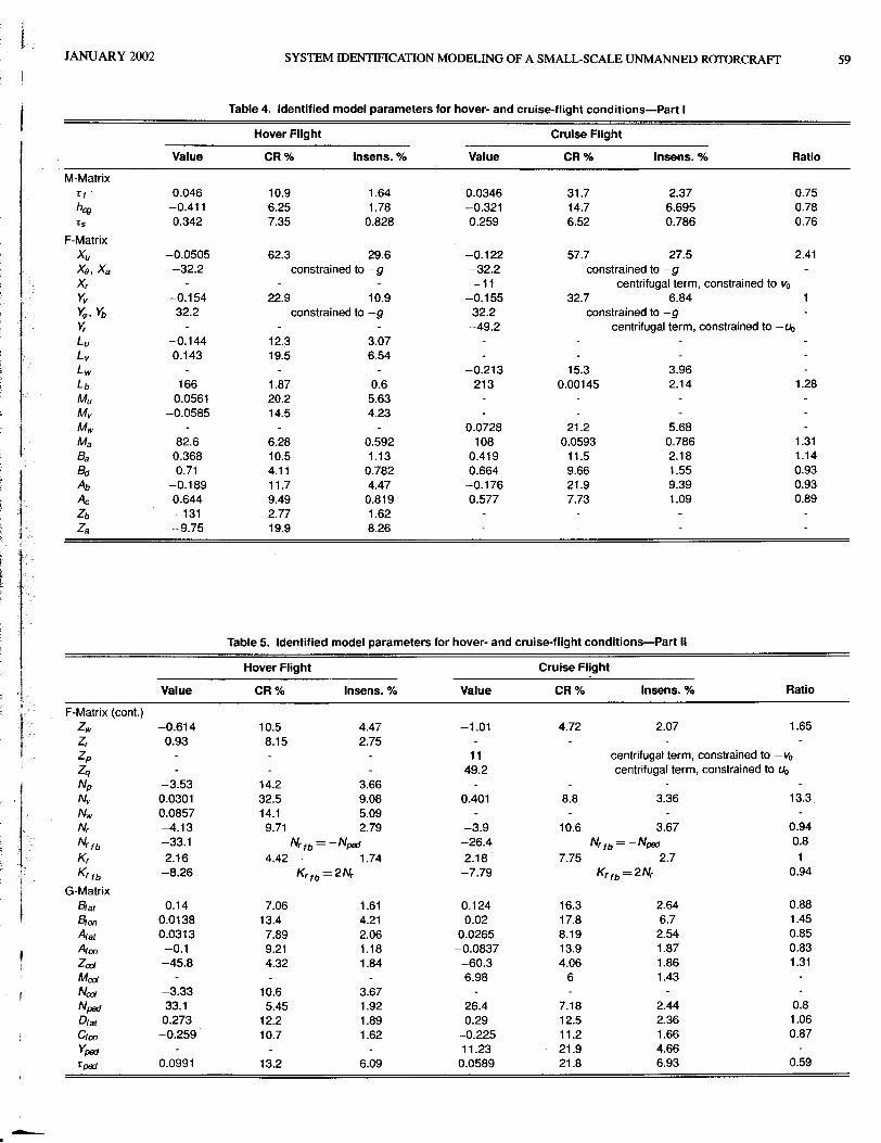
Tables 4 and 5 give the values of the identified derivatives as well where u is rotor soliditY, and Vo is inflow ratio derived from the thrustas two statistical metrics: the Cramer-Rao percent (CR%) and the insen- coefficient (vo = ~). These results also validate the results from

sitivity (Insens.%). The values of these metrics indicate that all of the the earlier work (Ref. 15), where the main rotor and stabilizer bar werekey control and response parameters are extracted with a high degree of modeled as a lumped system. It can now be stated that the time constantsprecision (Ref. 10). Notice that most of the quasi-steady derivatives are identified at the time (t" =0.38 sec) belonged to the stabilizer bar. Thisdropped, thus showing that the rotor forces dominate the dynamics of identification shows that the stabilizer bar dominates the rotor response.small-scale helicopters. This dominance is also reflected by the number In cruise condition the rotor time constants decrease to t"s = 0.26 sec andof rotor flapping derivatives ( )b and ( )a. The term actuated helicopter is t" f = 0.035 sec.a good idealization of the dynamics of the small-scale helicopter, wherethe rotor dominates the response. Coupling derivatives. The stabilizer bar couples to the main rotor through

the derivatives Bd and Ac. Application of Eq. (15), gives the equiv-Rotor parameters. The identified stabilizer-bar and main-rotor time con- alent Bell-mixer gearing. The results of Kd = 10.92 and Kc = 12.88slants for the hover conditions are t"s = 0.34 sec and t" f = 0.046 sec, for, respectively, the lateral and longitudinal axes, are close to the realrespectivelly. These values are close to the theoretical values of gearing K = 13.58 determined experimentally. In forward flight, the

"!

jJANUARY 2002 SYSTEM IDENTIFICATION MODELING OF A SMALL-SCALE UNMANNED ROTORCRAFr 59

i

t Table 4. Identified model parameters for hover- and cruise-flight conditions-Part I

Hover Flight Cruise Flight

I Value CR % Insens. % Value CR % Insens. % Ratio

M-Matrix'f 0.046 10.9 1.64 0.0346 31.7 2.37 0.75hcg -0.411 6.25 1.78 -0.321 14.7 6.695 0.78'5 0.342 7.35 0.828 0.259 6.52 0.786 0.76

F-MatrixXu -0.0505 62.3 29.6 -0.122 57.7 27.5 2.41Xe, Xa -32.2 constrained to -g -32.2 constrained to -gX, -11 centrifugal term, constrained to Vo

'Yv -0.154 22.9 10.9 -0.155 32.7 6.84 1r ~, Yb 32.2 constrained to -g 32.2 constrained to -gI Y;: - -49.2 centrifugal term, constrained to -Uo, Lu -0.144 12.3 3.07 --

Lv 0.143 19.5 6.54 -

Lw -0.213 15.3 3.96Lb 166 1.87 0.6 213 0.00145 2.14 1.28Mu -0.0561 20.2 5.63

, Mv -0.0585 14.5 4.23" Mw - 0.0728 21.2 5.68

Ma 82.6 6.28 0.592 108 0.0593 0.786 1.31.. Ba 0.368 10.5 1.13 0.419 11.5 2.18 1.14.I B<t 0.71 4.11 0.782 0.664 9.66 1.55 0.93

~ -0.189 11.7 4.47 -0.176 21.9 9.39 0.93Ac 0.644 9.49 0.819 0.577 7.73 1.09 0.89

J Zb -131 2.77 1.62Za -9.75 19.9 8.26

\

' I Table 5. Identified model parameters for hover- and cruise-flight conditions-Part II

Hover Flight Cruise FlightI Value CR % Insens. % Value CR % - Insens. % Ratio

.I F-Matrix (cont.) Zw -0.614 10.5 4.47 -1.01 4.72 2.07 1.65

l Z, 0.93 8.15 2.75 "

Zp 11 centrifugal term, constrained to -Voj Zq - 49.2 centrifugal term, constrained to Uo

I Np -3.53 14.2 3.66 -Nv 0.0301 32.5 9.08 0.401 8.8 3.36 13.3Nw 0.0857 14.1 5.09 -N, -4.13 9.71 2.79 -3.9 10.6 3.67 0.94N'fb -33.1 N'fb=-Np«i -26.4 N'fb=-Np«i 0.8K, 2.16 4.42 1.74 2.18 7.75 2.7 1

:'j K'fb -8.26 K'fb=2N, -7.79 K'fb=2N, 0.94"j G-MatrixI Stal 0.14 7.06 1.61 0.124 16.3 2.64 0.88

Ston 0.0138 13.4 4.21 0.02 17.8 6.7 1.45AlaI 0.0313 7.89 2.06 0.0265 8.19 2.54 0.85

I Alon -0.1 9.21 1.18 -0.0837 13.9 1.87 0.83J Zaj -45.8 4.32 1.84 -60.3 4.06 1.86 1.31

Maj - 6.98 6 1.43

I Naj -3.33 10.6 3.67Np«i 33.1 5.45 1.92 26.4 7.18 2.44 0.8DIal 0.273 12.2 1.89 0.29 12.5 2.36 1.06

i CIon -0.259 10.7 1.62 -0.225 11.2 1.66 0.87Yp«i 11.23 21.9 4.66'p«i 0.0991 13.2 6.09 0.0589 21.8 6.93 0.59

-.

60 B. METfLER JOURNAL OF THE AMERICAN HELICOIYrER SOCIETY

~ ;j:::I~::::~:=::;:::l::~ fu :t:~:::~~:~c= ~; t::;~==:~~~::_~=

- :t~~:~~~~~::'~:~::~ ~ r=::=:==~~:~~~:::: j=:::~~~~:~::=~:::::::: t::=~==:::=~.:===

:E:= b:;::: E= r=:==========

:t=:~::~:~::::::~~ = t~:~~==:::::::=~ j==~:~=:==::::::= t~~:~:=:::::~:~~:

:t~=~::===:=:::~ : [=~;;:~::~:~~::~: t~~.~~===~::::== t~:==::::==~::::

;!~~:~~:~::~==:: = t~:~~~=:==:~:=: t~:~:~:::::::~:~= t~~~~:~~::::::~:~:, .

~t====:=:ax (ft/s2) t=::~~~~ax (ft/s2) ~ \II (deg) . ~ t~~:::::::;:===;L:\II (deg) 0 - 0 t===:~~:==c0 ~ -

~ A- D0N 0 0. ~ ~

:t~~~:~~::::::{ ~ t=:~~=:~=~:~==: :t;~~=:~:~~:::: ~: r::~::~=:=::::=:0 I 2 3 4 5 6 0 I 2 3 4 5 6'0 1 2 3 4 5 6' 0 I 2 3 4 5 6

Time (s) Time (s) Time (s) Time (s)

Fig. 9. Comparison between the responses predicted by the identified hover model (dashed) and the responses obtained during flight testing inhover condition (solid).

~-

JANUARY 2002 SYSTEM IDENTIFICATION MODELING OF A SMALL-SCALE UNMANNED RafORCRAFT 61

! . ;1::I;~~~~~;O",,"_L~~~ lli :t~::~~~:~~:::= ,:t:~:=:==~~~~~:::~:

; , ";'

ii ~~~::=~~(j) (deg) ht~~:::~~==(j) (deg)t~======(j) (deg) (j) (deg)~' t~:=::== . c..' '" 0 ..., --- /i ~ ..'i! :L~-=- h :~g) ~=)--~ ( . == 1 ,:~::::=:::::~::: t===:== t:=====:=jr~,~ ~t~~~=~=[p (deg/s)t~~:===p (deg/s)t::=::=:::p (deg/s)t==::~::::p (deg/S)J!c"." II -,;I0 . -v -0I ...,, ,I:E::::: ~ E::= r=:~::=:::::::i ;t~~~~~=:::=:=: t~:~~~=~===::~:= l:== t~~:~:::~=~~==~: :r::~~::::::=: t~~::::~~::::::: t:::::=:l;~:~:::;o;,;,;['::: :, .I:t~:::~:::~~:~~: l~:~:;::~:~::2 ~ t~:~~::::=::::'0 1 2 3 4 5 0 I 2 3 4 5 0 I 2 3 4 5 0 I 2 3 4 5TlnIe (s) Tillie (s) Time (s) T~ (s)

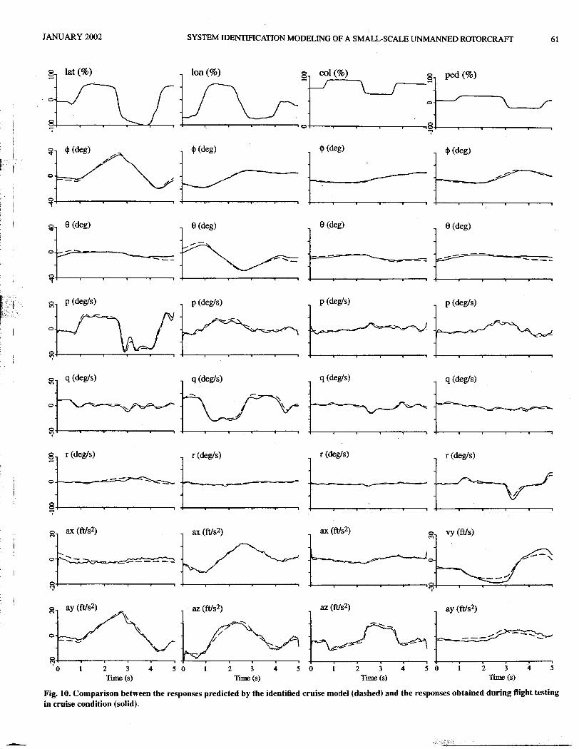
Fig. to. Comparison between the responses predicted by the identified cruise model (dashed) and the responses obtained during flight testingin cruise condition (solid).-- '!i!';!,

62 B. METTLER JOuRNAL OF THE AMERICAN HELICOfYrER SOCIETY

equivalent gearing results are: Kd = 10.73 and Kc = 13.79, and agree flight. Both results are anticipated. A time delay of 0.099 sec is identifiedwith the reality that the gearing is a mechanical constant. The identi- to account for the unmodeled high-frequency dynamics.fied roll and pitch rotor spring derivatives are, respectively, Lb = 166.1and Ma = 82.57, for hover conditions. These values for cruise condi- Heave dynamics. The heave damping derivative Zw has the correct sign.tion are about 30% larger: Lb = 213.2 and Ma = 108. The lateral and In cruise flight, the larger heave damping and heave control sensitivitylongitudinal main rotor control derivatives have reasonable values with Zco/ are anticipated. The latter is directly related to the reduction in in-only slight changes between hover and cruise conditions. The only ex- duced velocity in cruise flight.ception is B1on, which is 45% larger in cruise flight, indicating a highercross axis activity. The stabilizer bar control derivatives are almost iden- Time domain verificationtical for both flight conditions. These physically meaningful resultsindicat~ that the hybrid model structure with the stabilizer bar aug- For the time domain verification special flight experiments usingmenta~on accurately captures the coupled fuselage/rotor/stabilizer bar doublet-like control inputs are perfo~ed in hover and forward flight.dynamIcs. The recorded inputs are used as inputs to the identified model, and the

model-predicted responses are compared with the recorded helicopterQuasi-steady and speed derivatives. The speed derivatives Xu, and Y v, responses. For both the hover and cruise conditions, the results fromin the translational equations, Eqs. (3) and (4), have the sign and rel- the comparison are presented in Figs. 9 and 10, and overall, excellentative magnitudes expected for a hovering helicopter, but the absolute agreement is achieved.magnitudes are all considerably larger (2-5 times) than those for full Two areas exhibit some missmatch between model-predicted and ac-scale aircraft. This is expected since the weight of the small-scale he:. tual recorded responses: first, in the yaw rate response to the lateral cycliclicopters is proportionally smaller (weight scales by 1/ N3). In cruise input for the hover condition (Fig. 9); second, in the lateral velocity re-flight, the longitudinal speed derivative Xu increases significantly. Note sponse to the directional input for the cruise condition (Fig. 10). Notethat this derivative has the highest insensitivity of all the derivatives that both missmatches involve the lateral directional dynamics. Further-(29.6 and 27.5 for, respectively, hover and cruise flight), as well as a more, the accuracy of the identified linear model is excellent for largevery high Cramer-Rao values. Therefore, the identified value is unreli- attitudes and large excursions from the nominal operating conditions. Forable. This weak result is due to the insufficient low-frequency informa- example, the helicopter reac:hes bank angles up to 40 degrees and pitchtion content of the flight data caused by the short flight-data sequences attitudes up to 20 degrees. Note also that the cruise-flight experiments(10 sec). covered a range from 30 to 60 ft/sec (10 to 20 rn/sec).

The speed derivatives L u, Lv, M u and M v in angular rate equations,Eqs. (5) and (6), contribute a destabilizing influence on the phugoid Eigenvalues and dynamic modesdynamics. These derivatives are dropped for the cruise conditions becauseof excessive Cramer-Rao values . . .

. h' Important dynamIc charactenstics of the R-50 can be understood:WIt.h t e help of th~ offset Equ~tions (25) and (26), the force coupling from eigenvalues and eigenvectors computed from the identified model.

denvatives are constraIned to gravIty (- X = Yb =g) At the same time .. ..a. 'Tables 6 and 7 lIst the eIgenvalues and the dynamIc modes obtaIned forthe vertical C.G offset is identified to be hcg = -0.41 ft for hover and the hover and cruise conditions.hcg = -0.32 ft for cruise. The small difference of 0.09 ft (2.7 cm) is due Some of the modal characteristics can be related to the identifiedto changes in configuration and other unmodeled factors. derivatives. For example, the frequency of the pitch and roll coupled

fuselage/rotor/stabilizer modes can be related to the square root of theYaw dynamics. Little can be said with regard to the yaw dynamics because pitch flap spring (.,fM;; = 9.1 rad/sec) and the square root of the roll flapof the approximations used. Note that the yaw damping has the correct spring (~ = 12.9 rad/sec), respectively. Moreover, it can be shown thatnegative sign, and that the yaw rate feedback coefficients stay virtually the small damping ratio of these modes directly reflects the large effectiveconstant between hover and cruise conditions. The major changes are rotor time constant introduced by the stabilizer bar; for example, in thethose affecting the yaw control derivative N ped, which decreases, and roll axis: 'l;ro/l- flap = 2Ts~ = 0.11, and in the pitch axis: 'l;pilch- flap =the lateral speed derivative N v, which increases significantly in forward 2Ts.,fM;; = 0.16.

Table 6. Eigenvalues and modes in hover-flight condition

Eigenvalue Location Mode Description

}.1.2 0.306:1: 0.094i Unstable, damped, long period oscillatory, phugoid type mode. The main components are the(~ = -0.96; (J) = 0.32 rad/sec) longitudinal and lateral velocities and the roll and pitch angles

}.3.4 -0.401 :I: 0.086i Damped, long period oscillatory, phugoid type mode. The main components are the longitudinal(~ = 0.98; (J) = 0.41 rad/sec) and lateral velocities, the vertical velocity, and the roll, pitch, and yaw angles

}.5 -0.608 Damped yaw-heave mode}.6.7 -1.7 :I: 8.19i Lightly damped short period pitch mode. The main components are the pitch and roll rate. The mode

(~ = 0.20; (J) = 8.4 rad/sec) has a 25% roll rate component. This mode is related to the coupledfuselage/rotor/stabilizer bar dynamics

}.8.9 -6.2:1: 8.2i Underdamped short period yaw mode (effect of active yaw damping)(~ = 0.60; (J) = 10.3 rad/sec)

}.10.11 -2.66:1: 11.6i Lightly damped short period roll mode. The main components are the roll rate, the yaw rate and the(~ = 0.22; (J) = 11.9 rad/sec) pitch rate. This mode is related to the coupled fuselage/rotor/stabilizer bar dynamics

}.12,13 -20.2:1: 4.7i Nearly critically damped short period oscillatory roll mode. The main components are the roll and(~ = 0.97; (J) = 20.7 rad/sec) pitch (40%) rate. This mode is related to the coupled fuselage/rotor/stabilizer bar dynamics

"-~'- -

JANUARY 2002 SYSTEM IDENTIFICATION MODELING OF A SMALL-SCALE UNMANNED ROTORCRAFT 63

Table 7. Eigenvalues and modes in cruise-flight condition

Eigenvalue Location Mode Description

; A1 0.122 Damped longitudinal modeI ,A2 -0.96 Damped yaw-heave mode with a component of roll motion.. A3 -1.84 Damped lateral-directional mode 0 .

.t A45 -2.32:i: 8.79i Lightly damped short period pitching mode with a large (90%) rolling component. ThIs mode ISi' (t, = 0.26; w = 9.1 rad/sec) related to the coupledofuselagoe/rotor/stabili~er bar dynam!cs

t. A6.7 -5.0:i: 8.13i Underdamped short period yawIng mode (active yaw damping effect)I (t, =0.52;w=9.5 rad/sec) 0 0

A8.9 -3.4:i: 12.4i Lightly damped short period rolling mode with a small (10%) pitching component. This mode IS. (" = 0.26; w = 12.9 rad/sec) related to the coupled fuselage/rotor/stabilizer bar dynamics

A10.11 -27.04:i: 7.02i Nearly critically damped short period rolling mode with a 40% pitching component(t, = 0.97;w = 27.9 rad/sec)

Concluding Remarks 2Fletcher, J. W., "Identification ofUH-60 Stability Derivative Modelsin Hover from Flight Test Data," Journal of the American Helicopter

A parameterized model of a small-scale rotorcraft dynamics was de- Society, Vol. 40, (1), 1995.

velopedandsuccessfullyidentifiedusingfrequencydomainidentification 3Morris, J., Nieuwstadt, M. V., and Bendotti, P., "Identification andmethods. The key results are: Control of a Model Helicopter in Hover," Proceedings of the American

1) A coupled fuselage-rotor model based on the hybrid model formu- Control Conference, June 1994.lation, augmented to account for the presence of a stabilizer bar, allows 4Bruce,P. B., Silva, J. E. F., and Kellett, M.G., "Maximum Likelihoodan accurate fit of the frequency responses derived from the flight data for Identification of a Rotary-Wing RPV Simulation Model From Flight-Testboth hover and cruise conditions. Data," AIAA Paper No. 98-4157, Proceedings of the AIAA Atmospheric

2) The identification results are better than what is usually attained Flight Mechanics Conference and Exhibit, Boston, MA, 1998.in full-scale identification. The dynamics of the R-50 are governed by 5 Amidi, 0., Kanade, T., and Miller, R., "Vision-based Autonomousfirst-order effects; the rotor forces and moments dominate the dynamics. Helicopter Research at Carnegie Mellon Robotics Institute," Proceedings

3) The model has a minimum number of parameters. Most of which of Heli Japan'98, Japan, April 1998.have a well defined physical meaning. This enabled the extraction of 6Johnson, W.,HelicopterTheory, Dover Publications, New York, NY,key system parameters, including the main rotor and stabilizer bar time 1994, Chapter 15.constants"[ f and "[s, the stabilizer bar gearings Kc and Kd, and the flapping 7Heffley, R. K., "Compilation and Analysis of Helicopter Handlingspring derivatives L b and Ma. Qualities Data; Volume I: Data Compilation," Technical Report CR -3144,

4) Time domain verification showed that the model accuratl y predicts NASA, 1979.the response of the helicopter to control inputs. The identified model 8Langhaar, H. L., Dimensional Analysis and Theory of Models, Johnshould be well suited to flight control design, handling quality evaluation, Wiley & Sons, New York, 1951.and simulation applications. 9Padfield, G. D., Helicopter Flight Dynamics: The Theory and Ap-

5) The validation of the value of the key model parameters by heli- plication of Flying Qualities and Simulation Modeling, AIAA Educationcopter theory demonstrates that the model is physicaly meaningful and Series, Washington, 1996, pp. 38-40.should be applicable to the identification of other small-scale helicopters. loHam, J. A., Gardner, G. K., and Tischler, M. B., "Flight-Testing and

6) To improve the identification of the quasi-steady derivatives, longer Frequency-Domain Analysis for Rotorcraft Handling Qualities," Jour-flight-data sequences should be used in the future. This will require be tter nal of the American Helicopter Society, Vol. 40, (2), 1995, pp. 28-flight test techniques for the collection of flight data in cruise conditions. 38.

II Tomashofski, C. A., and Tischler, M. B., "Flight Test Identification

of SH-2G Dynamics in Support of Digital Flight Control System Devel-Acknowledgments . . . A 1 F P d .

opment," Amencan Helicopter Society 55th nnua orum rocee mgs,

0 A .do M k D L . d Montreal, Canada, May 1999.The authors are grateful to Drs. mead ml I, ar e OUIS an 12B d t J S d P. I A G E . eering Annlications Oif Corre- . . I , 50 .lbl d " hl . ena,..,an lerso,..,ngm ,..,..

RyanMillerformakmgCamegleMelonsR- avala ean lor epmg ,. dS ' A '. J h Wil &S New " ork NY 19930 . 0 ,atlon an pectra, na'YSlS, 0 n I ey ons., "" ,with the collection of the flight data. This work was supported by Yamaha 43-77Motor Corporation and by NASA under Grant NAG2-1276. PPi3H .

R S "T d B tte Understanding of Helicopter Sta-ansen, . ., .owar a e rbility Derivatives," Journal of the American Helicopter Society, Vol. 29,

References (1), 1982, pp. 15-24.14Chen, R., "Effects of Primary Rotor Parameters on Flapping Dy-

I Tischler, M. B., and Cauffman, M. G., "Frequency-Response namics," Technical Report TP-1431, NASA, 1980.

Method for Rotorcraft System Identification: Flight Application to 15Mettler, B., Tischler, M. B., and Kanade, T., "System IdentificationBO-I05 Coupled Rotor/Fuselage Dynamics," Journal of the American of Small-Size Unmanned Helicopter Dynamics," American HelicopterHelicopter Society, Vol. 37, (3), 1992, pp. 3-17. Society 55th Annual Forum Proceedings, Montreal, Canada, May 1999.

~