bernek noise control

CHAPTER 1

Basic Acoustical Quantities: Levelsand Decibels

LEO L. BERANEK

ConsultantCambridge, Massachusetts

1.1 BASIC QUANTITIES OF SOUND WAVES

Sound Waves and Noise

In the broadest sense, a sound wave is any disturbance that is propagated inan elastic medium, which may be a gas, a liquid, or a solid. Ultrasonic, sonic,and infrasonic waves are included in this definition. Most of this text deals withsonic waves, those sound waves that can be perceived by the hearing sense of ahuman being. Noise is defined as any perceived sound that is objectionable to ahuman being. The concepts basic to this chapter can be found in references 1–7.Portions are further expanded in Chapter 2.

Sound Pressure

A person who is not deaf perceives as sound any vibration of the eardrum in theaudible frequency range that results from an incremental variation in air pressureat the ear. A variation in pressure above and below atmospheric pressure is calledsound pressure, in units of pascals (Pa).∗ A young person with normal hearingcan perceive sound in the frequency range of roughly 15 Hz (hertz) to 16,000 Hz,defined as the normal audible frequency range.

Because the hearing mechanism responds to sound pressure, it is one of twoquantities that is usually measured in engineering acoustics. The normal ear ismost sensitive at frequencies between 3000 and 6000 Hz, and a young person candetect pressures as low as about 20 µPa, which, when compared to the normalatmospheric pressure (101.3 × 103 Pa) around which it varies, is a fractionalvariation of 2 × 10−10.

∗One pascal (Pa) = 1 newton/meter squared (N/m2) = 10 dynes/cm2

1

COPYRIG

HTED M

ATERIAL

2 BASIC ACOUSTICAL QUANTITIES: LEVELS AND DECIBELS

Pure Tone

A pure tone is a sound wave that can be represented by the equation,

p(t) = p0 sin(2πf )t (1.1)

where p(t) is the instantaneous, incremental, sound pressure (above and belowatmospheric pressure), p0 is the maximum amplitude of the instantaneous soundpressure, and f is the frequency, that is, the number of cycles per second,expressed in hertz. The time t is in seconds.

Period

A full cycle occurs when t varies from zero to 1/f . The 1/f quantity is knownas the period T . For example, the period T of a 500-Hz wave is 0.002 sec.

Root-Mean-Square Amplitude

If we wish to determine the mean value of a full cycle of the sine wave ofEq. (1.1.) (or any number of full cycles), it will be zero because the positivepart equals the negative part. Thus, the mean value is not a useful measure. Wemust look for a measure that permits the effects of the rarefactions to be addedto (rather than subtracted from) the effects of the compressions.

One such measure is the root-mean-square (rms) sound pressure prms. It isobtained, first, by squaring the value of the sound pressure disturbance p(t) ateach instant of time. Next the squared values are added and averaged over oneor more periods. The rms sound pressure is the square root of this time average.The rms value is also called the effective value. Thus

p2rms = 1

2p20 (1.2)

orprms = 0.707p0 (1.3)

In the case of nonperiodic sound pressures, the integration interval should belong enough to make the rms value obtained essentially independent of smallchanges in the length of the interval.

Sound Spectra

A sound wave may be comprised of a pure tone (single frequency, e.g., 1000 Hz),a combination of single frequencies harmonically related, or a combination ofsingle frequencies not harmonically related, either finite or infinite in number.A combination of a finite number of tones is said to have a line spectrum. Acombination of an infinite (large) number of tones has a continuous spectrum.A continuous-spectrum noise for which the amplitudes versus time occur with a

BASIC QUANTITIES OF SOUND WAVES 3

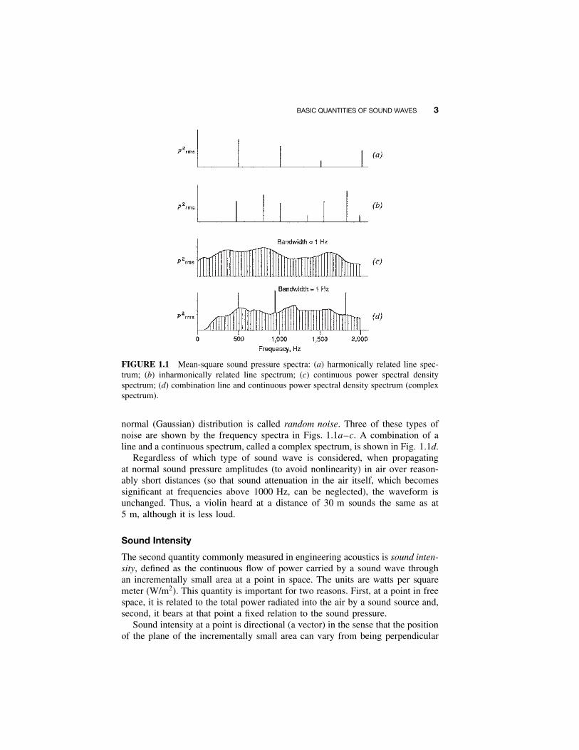
FIGURE 1.1 Mean-square sound pressure spectra: (a) harmonically related line spec-trum; (b) inharmonically related line spectrum; (c) continuous power spectral densityspectrum; (d) combination line and continuous power spectral density spectrum (complexspectrum).

normal (Gaussian) distribution is called random noise. Three of these types ofnoise are shown by the frequency spectra in Figs. 1.1a–c. A combination of aline and a continuous spectrum, called a complex spectrum, is shown in Fig. 1.1d.

Regardless of which type of sound wave is considered, when propagatingat normal sound pressure amplitudes (to avoid nonlinearity) in air over reason-ably short distances (so that sound attenuation in the air itself, which becomessignificant at frequencies above 1000 Hz, can be neglected), the waveform isunchanged. Thus, a violin heard at a distance of 30 m sounds the same as at5 m, although it is less loud.

Sound Intensity

The second quantity commonly measured in engineering acoustics is sound inten-sity, defined as the continuous flow of power carried by a sound wave throughan incrementally small area at a point in space. The units are watts per squaremeter (W/m2). This quantity is important for two reasons. First, at a point in freespace, it is related to the total power radiated into the air by a sound source and,second, it bears at that point a fixed relation to the sound pressure.

Sound intensity at a point is directional (a vector) in the sense that the positionof the plane of the incrementally small area can vary from being perpendicular


to the direction in which the wave is traveling to being parallel to that direction.It has its maximum value, Imax, when its plane is perpendicular to the directionof travel. When parallel, the sound intensity is zero. In between, the componentof Imax varies as the cosine of the angle formed by the direction of travel and aline perpendicular to the incremental area.

Another equation, which we shall develop in the next chapter, relates soundpressure to sound intensity. In an environment in which there are no reflectingsurfaces, the sound pressure at any point in any type of freely traveling (plane,cylindrical, spherical, etc.) wave is related to the maximum intensity Imax by

p2rms = Imax · ρc Pa2 (1.4)

where prms = rms sound pressure, Pa (N/m2)ρ = density of air, kg/m3

c = speed of sound in air, m/s [see Eq. (1.7)]N = force, N

Sound Power

A sound source radiates a measurable amount of power into the surroundingair, called sound power, in watts. If the source is nondirectional, it is said to bea spherical sound source (see Fig. 1.2). For such a sound source the measured(maximum) sound intensities at all points on an imaginary spherical surfacecentered on the acoustic center of the source are equal. Mathematically,

Ws = (4πr2)Is(r) W (1.5)

where Is(r) = maximum sound intensity at radius r at surface of an imaginarysphere surrounding source, W/m2

Ws = total sound power radiated by source in watts, W (N · m/s)r = distance from acoustical center of source to surface of imaginary

sphere, m

A similar statement can be made about a line source; that is, the maximumsound intensities at all points on an imaginary cylindrical surface around a cylin-drical sound source, Ic(r), are equal:

Wc = (2πrl)Ic(r) W (1.6)

where Wc = total sound power radiated by cylinder of length l, Wr = distance from acoustical centerline of cylindrical source to

imaginary cylindrical surface surrounding source

Inverse Square Law

With a spherical source, the radiated sound wave is spherical and the total powerradiated in all directions is W . The sound intensity I (r) must decrease with

BASIC QUANTITIES OF SOUND WAVES 5

Area ofthe wavefrontat d1 (1 m)

The area of thewavefront is 4 timesgreater at d2 (2 m)

1 m 2 m

72 dB 66 dB

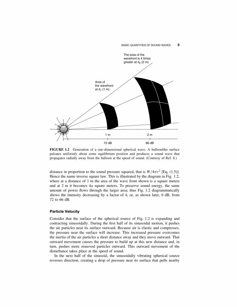
FIGURE 1.2 Generation of a one-dimensional spherical wave. A balloonlike surfacepulsates uniformly about some equilibrium position and produces a sound wave thatpropagates radially away from the balloon at the speed of sound. (Courtesy of Ref. 8.)

distance in proportion to the sound pressure squared, that is W/4πr2 [Eq. (1.5)].Hence the name inverse square law. This is illustrated by the diagram in Fig. 1.2,where at a distance of 1 m the area of the wave front shown is a square metersand at 2 m it becomes 4a square meters. To preserve sound energy, the sameamount of power flows through the larger area; thus Fig. 1.2 diagrammaticallyshows the intensity decreasing by a factor of 4, or, as shown later, 6 dB, from72 to 66 dB.

Particle Velocity

Consider that the surface of the spherical source of Fig. 1.2 is expanding andcontracting sinusoidally. During the first half of its sinusoidal motion, it pushesthe air particles near its surface outward. Because air is elastic and compresses,the pressure near the surface will increase. This increased pressure overcomesthe inertia of the air particles a short distance away and they move outward. Thatoutward movement causes the pressure to build up at this new distance and, inturn, pushes more removed particles outward. This outward movement of thedisturbance takes place at the speed of sound.

In the next half of the sinusoid, the sinusoidally vibrating spherical sourcereverses direction, creating a drop of pressure near its surface that pulls nearby


air particles toward it. This reverse disturbance also propagates outward withthe speed of sound. Thus, at any one point in space, there will be sinusoidalto-and-fro movement of the particles, called the particle velocity. Also at anypoint, there will be sinusoidal rise and fall of sound pressure.

From the basic equations governing the propagation of sound, as is shown inthe next chapter, we can say the following:

1. In a plane wave (approximated at a large distance from a point source)propagated in free space (no reflecting surfaces) the sound pressure andthe particle velocity reach their maximum and minimum values at the sameinstant and are said to be in phase.

2. In such a wave the particles move back and forth along the line in which thewave is traveling. In reference to the spherical radiation discussed above,this means that the particle velocity is always perpendicular to the imagi-nary spherical surface (the wave front) in space. This type of wave is calleda longitudinal, or compressional, wave. By contrast, a transverse wave isillustrated by a surface wave in water where the particle velocity is per-pendicular to the water surface while the wave propagates in a directionparallel to the surface.

Speed of Sound

A sound wave travels outward at a rate dependent on the elasticity and densityof the air. Mathematically, the speed of sound in air is calculated as

c =√

1.4Ps

ρm/s (1.7)

where Ps = atmospheric (ambient) pressure, Paρ = density of air, kg/m3

For all practical purposes, the speed of sound is dependent only on the absolutetemperature of the air. The equations for the speed of sound are

c = 20.05√

T m/s (1.8)

c = 49.03√

R ft/s (1.9)

where T = absolute temperature of air in degrees Kelvin, equal to 273.2plus the temperature in degrees Celsius

R = absolute temperature in degrees Rankine, equal to 459.7 plus thetemperature in degrees Fahrenheit

For temperatures near 20◦C (68◦F), the speed of sound is

c = 331.5 + 0.58◦C m/s (1.10)

c = 1054 + 1.07◦F ft/s (1.11)

SOUND SPECTRA 7

Wavelength

Wavelength is defined as the distance the pure-tone wave travels during a fullperiod. It is denoted by the Greek letter λ and is equal to the speed of sounddivided by the frequency of the pure tone:

λ = cT = c

fm (1.12)

Sound Energy Density

In standing-wave situations, such as sound waves in closed, rigid-wall tubes,rooms containing little sound-absorbing material, or reverberation chambers, thequantity desired is not sound intensity, but rather the sound energy density,namely, the energy (kinetic and potential) stored in a small volume of air in theroom owing to the presence of the standing-wave field. The relation between thespace-averaged sound energy density D and the space-averaged squared soundpressure is

D = p2av

ρc2= p2

av

1.4Ps

W · s/m3 (J/m3 or simply N/m2) (1.13)

where p2av = space average of mean-square sound pressure in a space,

determined from data obtained by moving a microphone alonga tube or around a room or from samples at various points, Pa2

Ps = atmospheric pressure, Pa; under normal atmospheric conditions,at sea level, Ps = 1.013 × 105 Pa

1.2 SOUND SPECTRA

In the previous section we described sound waves with line and continuousspectra. Here we shall discuss how to quantify such spectra.

Continuous Spectra

As stated before, a continuous spectrum can be represented by a large number ofpure tones between two frequency limits, whether those limits are apart 1 Hz orthousands of hertz (see Fig. 1.3). Because the hearing system extends over a largefrequency range and is not equally sensitive to all frequencies, it is customary tomeasure a continuous-spectrum sound in a series of contiguous frequency bandsusing a sound analyzer.

Customary bandwidths are one-third octave and one octave (see Fig. 1.4 andTable 1.1). The rms value of such a filtered sound pressure is called the one-third-octave-band or the octave-band sound pressure, respectively. If the filter bandwidthis 1 Hz, a plot of the filtered mean-square pressure of a continuous-spectrum


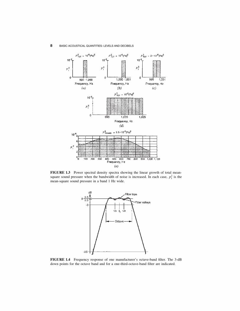
FIGURE 1.3 Power spectral density spectra showing the linear growth of total mean-square sound pressure when the bandwidth of noise is increased. In each case, p2

1 is themean-square sound pressure in a band 1 Hz wide.

FIGURE 1.4 Frequency response of one manufacturer’s octave-band filter. The 3-dBdown points for the octave band and for a one-third-octave-band filter are indicated.

SOUND SPECTRA 9

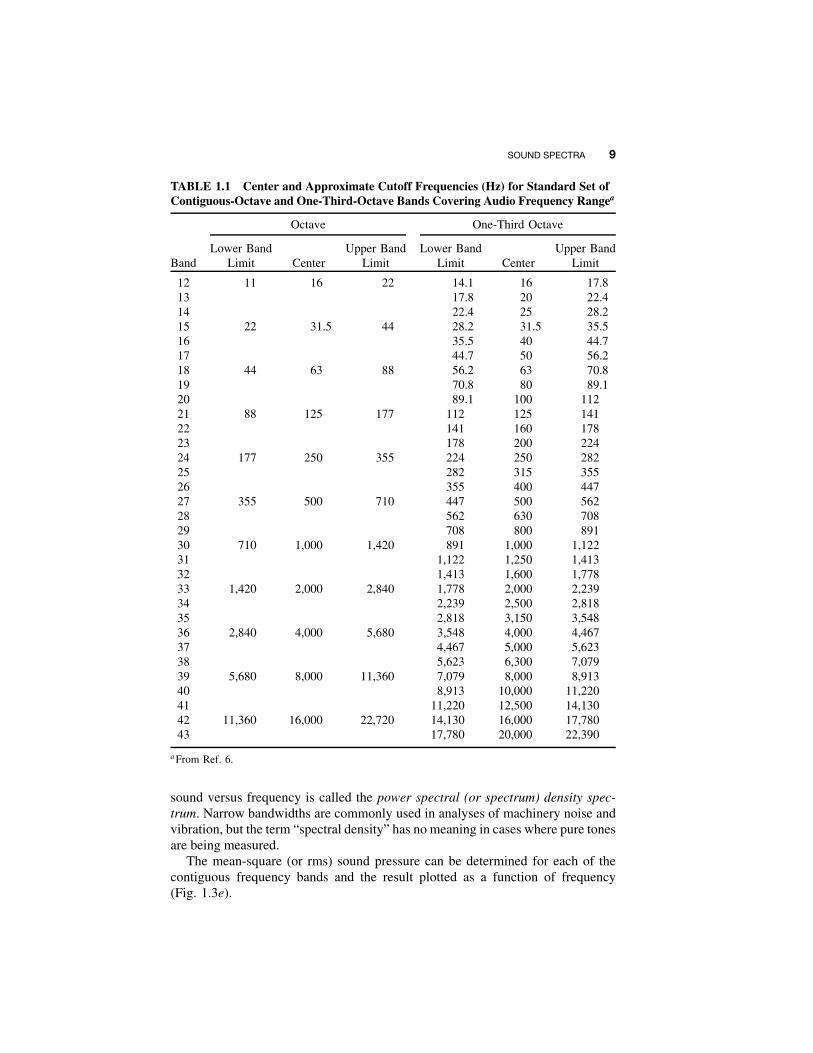
TABLE 1.1 Center and Approximate Cutoff Frequencies (Hz) for Standard Set ofContiguous-Octave and One-Third-Octave Bands Covering Audio Frequency Rangea

Octave One-Third Octave

BandLower Band

Limit CenterUpper Band

LimitLower Band

Limit CenterUpper Band

Limit

12 11 16 22 14.1 16 17.813 17.8 20 22.414 22.4 25 28.215 22 31.5 44 28.2 31.5 35.516 35.5 40 44.717 44.7 50 56.218 44 63 88 56.2 63 70.819 70.8 80 89.120 89.1 100 11221 88 125 177 112 125 14122 141 160 17823 178 200 22424 177 250 355 224 250 28225 282 315 35526 355 400 44727 355 500 710 447 500 56228 562 630 70829 708 800 89130 710 1,000 1,420 891 1,000 1,12231 1,122 1,250 1,41332 1,413 1,600 1,77833 1,420 2,000 2,840 1,778 2,000 2,23934 2,239 2,500 2,81835 2,818 3,150 3,54836 2,840 4,000 5,680 3,548 4,000 4,46737 4,467 5,000 5,62338 5,623 6,300 7,07939 5,680 8,000 11,360 7,079 8,000 8,91340 8,913 10,000 11,22041 11,220 12,500 14,13042 11,360 16,000 22,720 14,130 16,000 17,78043 17,780 20,000 22,390

a From Ref. 6.

sound versus frequency is called the power spectral (or spectrum) density spec-trum. Narrow bandwidths are commonly used in analyses of machinery noise andvibration, but the term “spectral density” has no meaning in cases where pure tonesare being measured.

The mean-square (or rms) sound pressure can be determined for each of thecontiguous frequency bands and the result plotted as a function of frequency(Fig. 1.3e).


Bandwidth Conversion. It is frequently necessary to convert sounds measuredwith one set of bandwidths to a different set of bandwidths or to reduce bothsets of measurements to a third set of bandwidths. Let us imagine that we havea machine that at a point in space produces a mean-square sound pressure ofp2

1 = 10−6 Pa2 in a 1-Hz bandwidth between 999 and 1000 Hz (Fig. 1.3a). Nowimagine that we have a second machine the same distance away that radiatesthe same power but is confined to a bandwidth between 1000 and 1001 Hz(Fig. 1.3b). The total spectrum now becomes that shown in Fig. 1.3c and thetotal mean-square pressure is twice that in either band. Similarly, 10 machineswould produce 10 times the mean-square sound pressure of any one (Fig. 1.3d).

In other words, if the power spectral density spectrum in a frequency band ofwidth �f is flat (the mean-square sound pressures in all the 1-Hz-wide bands,p2

1, within the band are equal), the total mean-square sound pressure for the bandis given by

p2tot = p2

1�f

�f0Pa2 (1.14)

where �f0 = 1 Hz.As an example, assume that we wish to convert the power spectral density

spectrum of Fig. 1.3e, which is a plot of p21(f ), the mean-square sound pressure

in 1-Hz bands, to a spectrum for which the mean-square sound pressure in 100-Hzbands, p2

tot, is plotted versus frequency. Let us consider only the 700–800-Hzband. Because p2

1(f ) is not equal throughout this band, we could painstakinglydetermine and add together the actual p2

1’s or, as is more usual, simply takethe average value for the p2

1’s in that band and multiply by the bandwidth.Thus, for each 100-Hz band, the total mean-square sound pressure is given byEq. (1.14), where p2

1 is the average 1-Hz band quantity throughout the band. Forthe 700–800-Hz band, the average p2

1 is 5.5 × 10−6 and the total is 5.5 × 10−6 ×100 Hz = 5.5 × 10−4 Pa2.

If mean-square sound pressure levels have been measured in a specific set ofbandwidths such as one-third-octave bands, it is possible to present accurately thedata in a set of wider bandwidths such as octave bands by simply adding togetherthe mean-square sound pressures for the component bands. Obviously, it is notpossible to reconstruct a narrower bandwidth spectrum accurately (e.g., one-third-octave bands) from a wider bandwidth spectrum (e.g., octave bands.) However,it is sometimes necessary to make such a conversion in order to compare sets ofdata measured differently. Then the implicit assumption has to be made that thenarrower band spectrum is continuous and monotonic within the larger band. Ineither direction, the conversion factor for each band is

p2B = p2

A

�fB

�fA

(1.15)

where p2A is the measured mean-square sound pressure in a bandwidth �fA and

p2B is the desired mean-square sound pressure in the desired bandwidth �fB .

SOUND SPECTRA 11

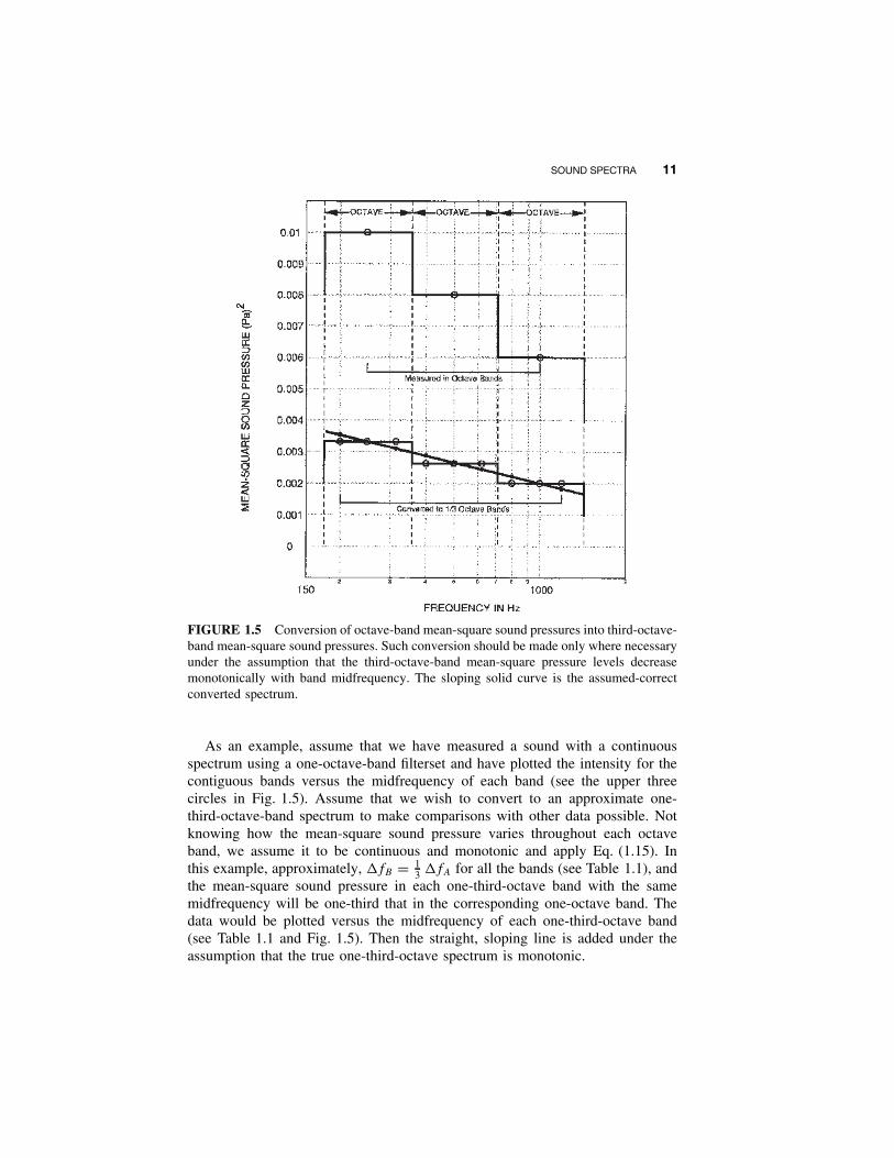
FIGURE 1.5 Conversion of octave-band mean-square sound pressures into third-octave-band mean-square sound pressures. Such conversion should be made only where necessaryunder the assumption that the third-octave-band mean-square pressure levels decreasemonotonically with band midfrequency. The sloping solid curve is the assumed-correctconverted spectrum.

As an example, assume that we have measured a sound with a continuousspectrum using a one-octave-band filterset and have plotted the intensity for thecontiguous bands versus the midfrequency of each band (see the upper threecircles in Fig. 1.5). Assume that we wish to convert to an approximate one-third-octave-band spectrum to make comparisons with other data possible. Notknowing how the mean-square sound pressure varies throughout each octaveband, we assume it to be continuous and monotonic and apply Eq. (1.15). Inthis example, approximately, �fB = 1

3 �fA for all the bands (see Table 1.1), andthe mean-square sound pressure in each one-third-octave band with the samemidfrequency will be one-third that in the corresponding one-octave band. Thedata would be plotted versus the midfrequency of each one-third-octave band(see Table 1.1 and Fig. 1.5). Then the straight, sloping line is added under theassumption that the true one-third-octave spectrum is monotonic.


Complex Spectra

The mean-square sound pressure resulting from the combination of two or morepure tones of different amplitudes p1, p2, p3 and different frequencies f1, f2, f3

is given byp2

rms(total) = p21 + p2

2 + p23 + · · · (1.16)

The mean-square sound pressure of two pure tones of the same frequency butdifferent amplitudes and phases is found from

p2rms(total) = p2

1 + p22 + 2p1p2 cos(θ1 − θ2) (1.17)

where the phase angle of each wave is represented by θ1 or θ2.Comparison of Eqs. (1.16) and (1.17) reveals the importance of phase when

combining two sine waves of the same frequency. If the phase difference θ1 − θ2

is zero, the two waves are in phase and the combination is at its maximumvalue. If θ1 − θ2 = 180◦, the third term becomes −2p1p2 and the sum is at itsminimum value. If the two waves are equal in amplitude, the minimum valueis zero.

If one wishes to find the mean-square sound pressure of a number of wavesall of which have different frequencies except, say, two, these two are addedtogether according to Eq. (1.17) to obtain a mean-square pressure for them. Thenthis mean-square pressure and the mean-square pressures of the remainder of thecomponents are summed according to Eq. (1.16).

1.3 LEVELS6

Because of the wide range of sound pressures to which the ear responds (aratio of 105 or more for a normal person), sound pressure is an inconvenientquantity to use in graphs and tables. This is also true for the other acousticalquantities listed above. Early in the history of the telephone it was decided toadopt logarithmic scales for representing acoustical quantities and the voltagesencountered in associated electrical equipment.

As a result of that decision, sound powers, intensities, pressures, velocities,energy densities, and voltages from electroacoustic transducers are commonlystated in terms of the logarithm of the ratio of the measured quantity to anappropriate reference quantity. Because the sound pressure at the threshold ofhearing at 1000 Hz is about 20 µPa, this was chosen as the fundamental referencequantity around which the other acoustical references have been chosen.

Whenever the magnitude of an acoustical quantity is given in this logarithmicform, it is said to be a level in decibels (dB) above or below a zero referencelevel that is determined by a reference quantity. The argument of the logarithm isalways a ratio and, hence, is dimensionless. The level for a very large ratio, forexample the power produced by a very powerful sound source, might be givenwith the unit bel, which equals 10 dB.

LEVELS 13

Power and Intensity Levels

Sound Power Level. Sound power level is defined as

LW = 10 log10W

W0dB re W0 (1.18)

and conversely

W = W0 antilog10LW

10= W0 × 10LW /10 W (1.19)

where W = sound power, W (watts)W0 = reference sound power, standardized at 10−12 W

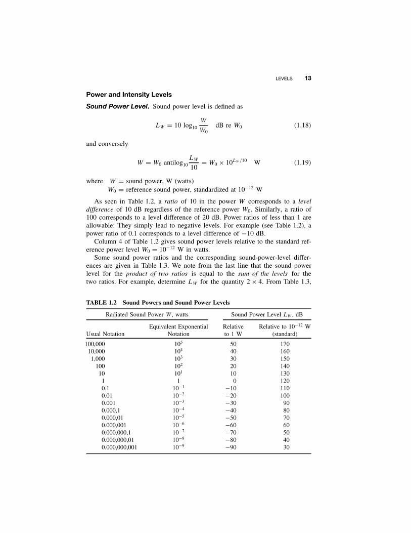
As seen in Table 1.2, a ratio of 10 in the power W corresponds to a leveldifference of 10 dB regardless of the reference power W0. Similarly, a ratio of100 corresponds to a level difference of 20 dB. Power ratios of less than 1 areallowable: They simply lead to negative levels. For example (see Table 1.2), apower ratio of 0.1 corresponds to a level difference of −10 dB.

Column 4 of Table 1.2 gives sound power levels relative to the standard ref-erence power level W0 = 10−12 W in watts.

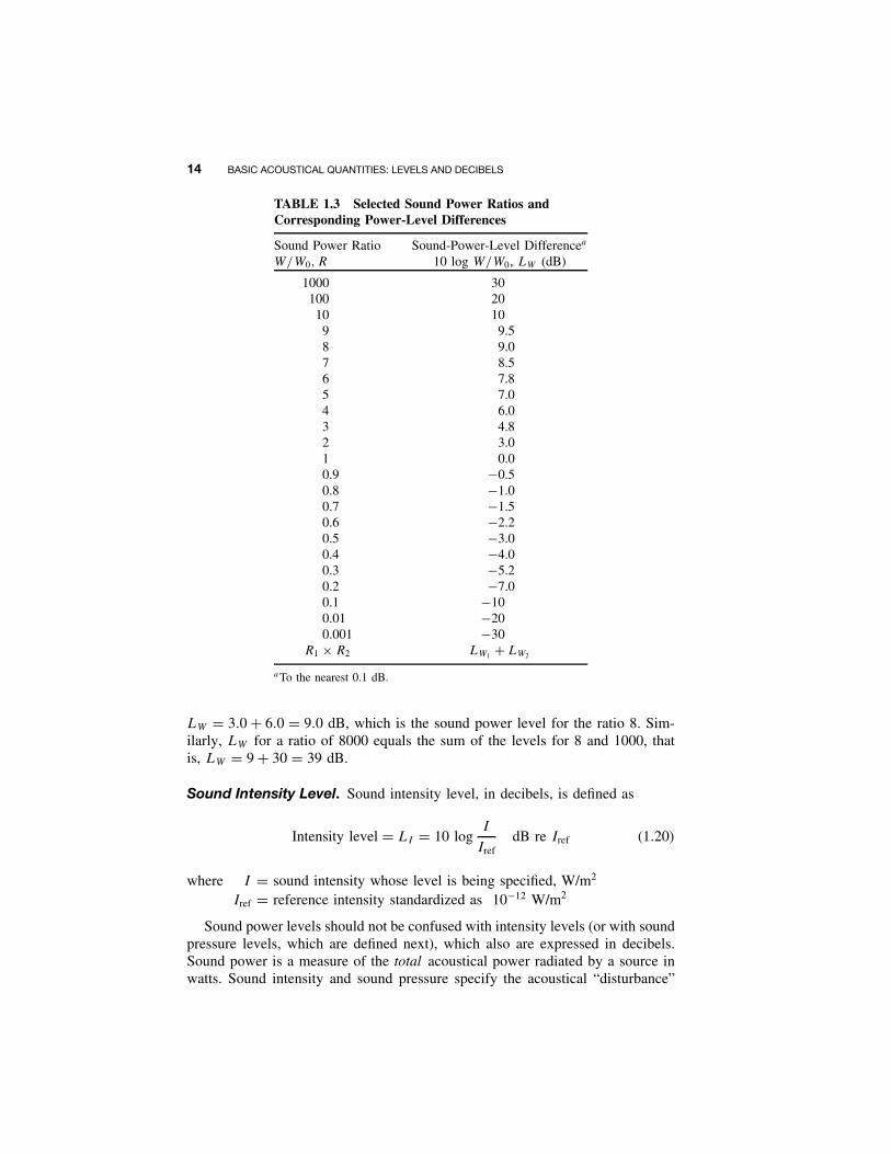
Some sound power ratios and the corresponding sound-power-level differ-ences are given in Table 1.3. We note from the last line that the sound powerlevel for the product of two ratios is equal to the sum of the levels for thetwo ratios. For example, determine LW for the quantity 2 × 4. From Table 1.3,

TABLE 1.2 Sound Powers and Sound Power Levels

Radiated Sound Power W , watts Sound Power Level LW , dB

Usual NotationEquivalent Exponential

NotationRelativeto 1 W

Relative to 10−12 W(standard)

100,000 105 50 17010,000 104 40 1601,000 103 30 150

100 102 20 14010 101 10 130

1 1 0 1200.1 10−1 −10 1100.01 10−2 −20 1000.001 10−3 −30 900.000,1 10−4 −40 800.000,01 10−5 −50 700.000,001 10−6 −60 600.000,000,1 10−7 −70 500.000,000,01 10−8 −80 400.000,000,001 10−9 −90 30


TABLE 1.3 Selected Sound Power Ratios andCorresponding Power-Level Differences

Sound Power RatioW/W0, R

Sound-Power-Level Differencea

10 log W/W0, LW (dB)

1000 30100 20

10 109 9.58 9.07 8.56 7.85 7.04 6.03 4.82 3.01 0.00.9 −0.50.8 −1.00.7 −1.50.6 −2.20.5 −3.00.4 −4.00.3 −5.20.2 −7.00.1 −100.01 −200.001 −30

R1 × R2 LW1 + LW2

a To the nearest 0.1 dB.

LW = 3.0 + 6.0 = 9.0 dB, which is the sound power level for the ratio 8. Sim-ilarly, LW for a ratio of 8000 equals the sum of the levels for 8 and 1000, thatis, LW = 9 + 30 = 39 dB.

Sound Intensity Level. Sound intensity level, in decibels, is defined as

Intensity level = LI = 10 logI

IrefdB re Iref (1.20)

where I = sound intensity whose level is being specified, W/m2

Iref = reference intensity standardized as 10−12 W/m2

Sound power levels should not be confused with intensity levels (or with soundpressure levels, which are defined next), which also are expressed in decibels.Sound power is a measure of the total acoustical power radiated by a source inwatts. Sound intensity and sound pressure specify the acoustical “disturbance”

DEFINITIONS OF OTHER COMMONLY USED LEVELS AND QUANTITIES IN ACOUSTICS 15

produced at a point removed from the source. For example, their levels depend onthe distance from the source, losses in the intervening air path, and room effects(if indoors). A helpful analogy is to imagine that sound power level is related tothe total rate of heat production of a furnace, while either of the other two levelsis analogous to the temperature produced at a given point in a dwelling.

Sound Pressure Level

Almost all microphones used today respond to sound pressure, and in the publicmind, the word decibel is commonly associated with sound pressure level or A-weighted sound pressure level (see Table 1.4). Strictly speaking, sound pressurelevel is analogous to intensity level, because, in calculating it, pressure is firstsquared, which makes it proportional to intensity (power per unit area):

Sound pressure level = Lp = 10 log

[p(t)

pref

]2

= 20 logp(t)

prefdB re pref (1.21)

where pref = reference sound pressure, standardized at 2 × 10−5 N/m2 (20 µPa)for airborne sound; for other media, references may be 0.1 N/m2

(1 dyn/cm2) or 1 µN/m2 (1 µPa)p(t) = instantaneous sound pressure, Pa

Note that Lp re 20 µPa is 94 dB greater than Lp re 1 Pa.As we shall show shortly, p(t)2 is only proportional to sound intensity if its

mean-square value is taken. Thus, in Eq. (1.21), p(t) would be replaced by prms.The relations among sound pressure levels (re 20 µPa) for pressures in the

meter-kilogram-second (mks), centimeter-gram-second (cgs), and English sys-tems of units are shown by the four nomograms of Fig. 1.6.

1.4 DEFINITIONS OF OTHER COMMONLY USED LEVELSAND QUANTITIES IN ACOUSTICS

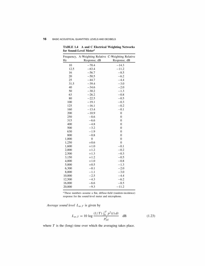
Analogous to sound pressure level given in Eq. (1.21), A-weighted sound pressurelevel LA is given by

LA = 10 log

[pA(t)

pref

]2

dB (1.22)

where pA(t) is the instantaneous sound pressure measured using the standardfrequency-weighting A (see Table 1.4).


TABLE 1.4 A and C Electrical Weighting Networksfor Sound-Level Metera

Frequency,Hz

A-Weighting RelativeResponse, dB

C-Weighting RelativeResponse, dB

10 −70.4 −14.312.5 −63.4 −11.216 −56.7 −8.520 −50.5 −6.225 −44.7 −4.431.5 −39.4 −3.040 −34.6 −2.050 −30.2 −1.363 −26.2 −0.880 −22.5 −0.5

100 −19.1 −0.3125 −16.1 −0.2160 −13.4 −0.1200 −10.9 0250 −8.6 0315 −6.6 0400 −4.8 0500 −3.2 0630 −1.9 0800 −0.8 0

1,000 0 01,250 +0.6 01,600 +1.0 −0.12,000 +1.2 −0.22,500 +1.3 −0.33,150 +1.2 −0.54,000 +1.0 −0.85,000 +0.5 −1.36,300 −0.1 −2.08,000 −1.1 −3.0

10,000 −2.5 −4.412,500 −4.3 −6.216,000 −6.6 −8.520,000 −9.3 −11.2

a These numbers assume a flat, diffuse-field (random-incidence)response for the sound-level meter and microphone.

Average sound level Lav,T is given by

Lav,T = 10 log(1/T )

∫ T

0 p2(t) dt

p2ref

dB (1.23)

where T is the (long) time over which the averaging takes place.

DEFINITIONS OF OTHER COMMONLY USED LEVELS AND QUANTITIES IN ACOUSTICS 17

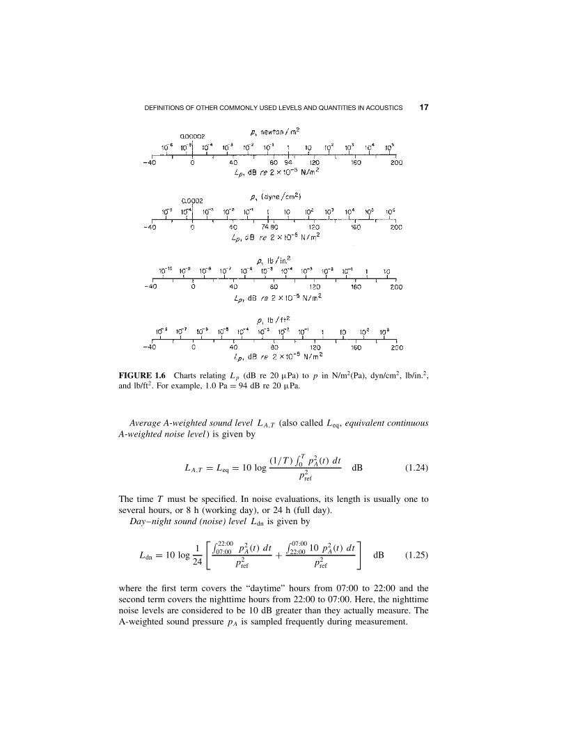
FIGURE 1.6 Charts relating Lp (dB re 20 µPa) to p in N/m2(Pa), dyn/cm2, lb/in.2,and lb/ft2. For example, 1.0 Pa = 94 dB re 20 µPa.

Average A-weighted sound level LA,T (also called Leq, equivalent continuousA-weighted noise level ) is given by

LA,T = Leq = 10 log(1/T )

∫ T

0 p2A(t) dt

p2ref

dB (1.24)

The time T must be specified. In noise evaluations, its length is usually one toseveral hours, or 8 h (working day), or 24 h (full day).

Day–night sound (noise) level Ldn is given by

Ldn = 10 log1

24

[∫ 22:0007:00 p2

A(t) dt

p2ref

+∫ 07:00

22:00 10 p2A(t) dt

p2ref

]dB (1.25)

where the first term covers the “daytime” hours from 07:00 to 22:00 and thesecond term covers the nighttime hours from 22:00 to 07:00. Here, the nighttimenoise levels are considered to be 10 dB greater than they actually measure. TheA-weighted sound pressure pA is sampled frequently during measurement.


A-weighted sound exposure EA,T is given by

EA,T =∫ t2

t1

p2A(t) dt Pa2 · s (1.26)

This equation is not a level. The term EA,T is proportional to the energy flow(intensity times time) in a sound wave in the time period T . The period T startsand stops at t1 and t2, respectively.

A-weighted noise exposure level LEA,T is given by

LEA,T = 10 log

(EA,T

E0

)dB (1.27)

where E0 is a reference quantity, standardized at (20 µPa)2 · s= (4 × 10−10 Pa)2 · s.However, the International Organization for Standardization standard ISO 1999:1990-01-5, on occupational noise level, uses E0 = (1.15 × 10−5 Pa)2 · s, because,for an 8-h day, LEA,T , with that reference, equals the average A-weighted soundpressure level LA,T . The two reference quantities yield levels that differ by 44.6 dB.For a single impulse, the time period T is of no consequence provided T is longerthan the impulse length and the background noise is low.

Hearing threshold for setting “zero” at each frequency on a pure-toneaudiometer is the standardized, average, pure-tone threshold of hearing for apopulation of young persons with no otological irregularities. The standardizedthreshold sound pressure levels at the frequencies 250, 500, 1000, 2000, 3000,4000, 6000, and 8000 Hz are, respectively, 24.5, 11.0, 6.5, 8.5, 7.5, 9.0, 8.0,and 9.5 dB measured under an earphone. An audiometer is used to determinethe difference at these frequencies between the threshold values of a person (thelowest sound pressure level of a pure tone the person can detect consistently)and the standardized threshold values. Measurements are sometimes also madeat 125 and 1500 Hz.7

Hearing impairment (hearing loss) is the number of decibels that the perma-nent hearing threshold of an individual at each measured frequency is abovethe zero setting on an audiometer, in other words, a change for the worseof the person’s threshold of hearing compared to the normal for youngpersons.

Hearing threshold levels associated with age are the standardized pure-tonethresholds of hearing associated solely with age. They were determined from testsmade on the hearing of persons in a certain age group in a population with nootological irregularities and no appreciable exposure to noise during their lives.

Hearing threshold levels associated with age and noise are the standardizedpure-tone thresholds determined from tests made on the hearing of individualswho had histories of higher than normal noise exposure during their lives. Theaverage noise levels and years of exposure were determined by questioning andmeasurement of the exposure levels.

Noise-induced permanent threshold shift (NIPTS) is the shift in the hearingthreshold level caused solely by exposure to noise.

REFERENCE QUANTITIES USED IN NOISE AND VIBRATION 19

1.5 REFERENCE QUANTITIES USED IN NOISE AND VIBRATION

American National Standard

The American National Standards Institute has issued a standard (ANSI S1.8-1989, Reaffirmed 2001) on “Reference Quantities for Acoustical Levels.” Thisstandard is a revision of ANSI S1.8-1969. The authors of this book have beensurveyed for their opinions on preferred reference quantities. Table 1.5 is a com-bination of the standard references and of references preferred by the authors.The two references are clearly distinguished. All quantities are stated in terms ofthe International System of units (SI) and in British units.

Relations among Sound Power Levels, Intensity Levels, and SoundPressure Levels

As a practical matter, the reference quantities for sound power, intensity, andsound pressure (in air) have been chosen so that their corresponding levels areinterrelated in a convenient way under certain circumstances.

The threshold of hearing at 1000 Hz for a young listener with acute hearing,measured under laboratory conditions, was determined some years ago as a soundpressure of 2 × 10−5 Pa. This value was then selected as the reference pressurefor sound pressure level.

Intensity at a point is related to sound pressure at that point in a free fieldby Eq. (1.14). A combination of Eqs. (1.4), (1.20), and (1.21) yields the soundintensity level

LI = 10 logI

Iref= 10 log

p2

ρcIref

= 10 logp2

p2ref

+ 10 logp2

ref

ρcIref

LI = Lp − 10 log K dB re 10−12 W/m2 (1.28)

where K = const = Irefρc/p2ref, which is dependent upon ambient pressure and

temperature; quantity 10 log K may be found from Fig. 1.7, or,K = ρc/400

The quantity 10 log K will equal zero, that is, K = 1, when

ρc = p2ref

Iref= 4 × 10−10

10−12= 400 mks rayls (1.29)

We may also rearrange Eq. (1.28) to give the sound pressure level

Lp = LI + 10 log K dB re 2 × 10−5 Pa (1.30)

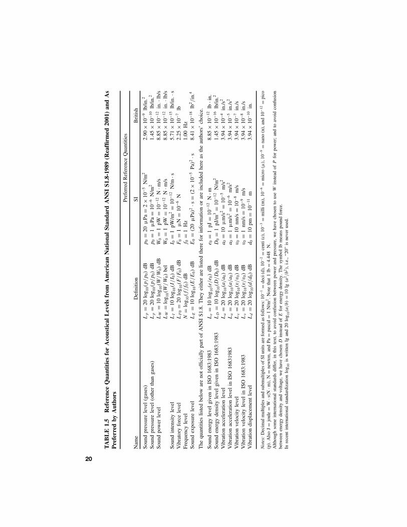
TA

BL

E1.

5R

efer

ence

Qua

ntit

ies

for

Aco

usti

cal

Lev

els

from

Am

eric

anN

atio

nal

Stan

dard

AN

SIS1

.8-1

989

(Rea

ffirm

ed20

01)

and

As

Pre

ferr

edby

Aut

hors

Pref

erre

dR

efer

ence

Qua

ntiti

es

Nam

eD

efini

tion

SIB

ritis

h

Soun

dpr

essu

rele

vel

(gas

es)

Lp

=20

log 1

0(p

/p

0)

dBp

0=

20µ

Pa=

2×

10−5

N/m

22.

90×

10−9

lb/in

.2

Soun

dpr

essu

rele

vel

(oth

erth

anga

ses)

Lp

=20

log 1

0(p

/p

0)

dBp

0=

1µ

Pa=

10−6

N/m

21.

45×

10−1

0lb

/in.2

Soun

dpo

wer

leve

lL

W=

10lo

g 10(W

/W

0)

dBW

0=

1pW

=10

−12

N·m

/s8.

85×

10−1

2in

.·lb

/sL

W=

log 1

0(W

/W

0)

bel

W0

=1

pW=

10−1

2N

·m/s

8.85

×10

−12

in.·lb

/sSo

und

inte

nsity

leve

lL

I=

10lo

g 10(I

/I 0

)dB

I 0=

1pW

/m2

=10

−12

N/m

·s5.

71×

10−1

5lb

/in.·s

Vib

rato

ryfo

rce

leve

lL

F0

=20

log 1

0(F

/F

0)

dBF

0=

1µ

N=

10−6

N2.

25×

10−7

lbFr

eque

ncy

leve

lN

=lo

g 10(f

/f0)

dBf

0=

1H

z1.

00H

zSo

und

expo

sure

leve

lL

E=

10lo

g 10(E

/E

0)

dBE

0=

(20

µPa

)2·s

=(2

×10

−5Pa

)2·s

8.41

×10

−18

lb2/in

.4

The

quan

titie

slis

ted

belo

war

eno

tof

ficia

llypa

rtof

AN

SIS1

.8.

The

yei

ther

are

liste

dth

ere

for

info

rmat

ion

orar

ein

clud

edhe

reas

the

auth

ors’

choi

ce.

Soun

den

ergy

leve

lgi

ven

inIS

O16

83:1

983

Le=

10lo

g 10(e

/e 0

)dB

e 0=

1pJ

=10

−12

N·m

8.85

×10

−12

lb·in

.So

und

ener

gyde

nsity

leve

lgi

ven

inIS

O16

83:1

983

LD

=10

log 1

0(D

/D

0)

dBD

0=

1pJ

/m3

=10

−12

N/m

21.

45×

10−1

6lb

/in.2

Vib

ratio

nac

cele

ratio

nle

vel

La

=20

log 1

0(a

/a

0)

dBa

0=

10µ

m/s

2=

10−5

m/s

23.

94×

10−4

in./s

2

Vib

ratio

nac

cele

ratio

nle

vel

inIS

O16

8319

83L

a=

20lo

g 10(a

/a

0)

dBa

0=

1µ

m/s

2=

10−6

m/s

23.

94×

10−5

in./s

2

Vib

ratio

nve

loci

tyle

vel

Lv

=20

log 1

0(v

/v

0)

dBv

0=

10nm

/s=

10−8

m/s

3.94

×10

−7in

./sV

ibra

tion

velo

city

leve

lin

ISO

1683

:198

3L

v=

20lo

g 10(v

/v

0)

dBv

0=

1nm

/s=

10−9

m/s

3.94

×10

−8in

./sV

ibra

tion

disp

lace

men

tle

vel

Ld

=20

log 1

0(d

/d

0)

dBd

0=

10pm

=10

−11

m3.

94×

10−1

0in

.

Not

es:

Dec

imal

mul

tiple

san

dsu

bmul

tiple

sof

SIun

itsar

efo

rmed

asfo

llow

s:10

−1=

deci

(d),

10−2

=ce

nti(

c),1

0−3=

mill

i(m

),10

−6=

mic

ro(µ

),10

−9=

nano

(n),

and

10−1

2=

pico

(p).

Als

oJ

=jo

ule

=W

·s(N

·m),

N=

new

ton,

and

Pa=

pasc

al=

1N

/m2.

Not

eth

at1

lb=

4.44

8N

.A

lthou

ghso

me

inte

rnat

iona

lst

anda

rds

diff

er,

inth

iste

xt,

toav

oid

conf

usio

nbe

twee

npo

wer

and

pres

sure

,w

eha

vech

osen

tous

eW

inst

ead

ofP

for

pow

er;

and

toav

oid

conf

usio

nbe

twee

nen

ergy

dens

ityan

dvo

ltage

,w

eha

vech

osen

Din

stea

dof

Efo

ren

ergy

dens

ity.

The

sym

bol

lbm

eans

poun

dfo

rce.

Inre

cent

inte

rnat

iona

lst

anda

rdiz

atio

nlo

g 10

isw

ritte

nlg

and

20lo

g 10(a

/b)=

10lg

(a2/b

2),

i.e.,

“20”

isne

ver

used

.

20

REFERENCE QUANTITIES USED IN NOISE AND VIBRATION 21

TABLE 1.6 Ambient Pressures and Temperatures for Which ρc(Air) = 400 mksrayls

Ambient Pressure Ambient Temperature T

ps ,Pa

m ofHg, 0◦C

in. ofHg, 0◦C ◦C ◦F

0.7 × 105 0.525 20.68 −124.3 −1920.8 × 105 0.600 23.63 −78.7 −1100.9 × 105 0.675 26.58 −27.0 −171.0 × 105 0.750 29.54 +30.7 +871.013 × 105 0.760 29.9 38.9 1021.1 × 105 0.825 32.5 94.5 2021.2 × 105 0.900 35.4 164.4 3281.3 × 105 0.975 38.4 240.4 4651.4 × 105 1.050 41.3 322.4 613

FIGURE 1.7 Chart determining the value of 10 log(ρc/400) = 10 log K as a functionof ambient temperature and ambient pressure. Values for which ρc = 400 are also givenin Table 1.6.

In Table 1.6, we show a range of ambient pressures and temperatures forwhich ρc = 400 mks rayls. We see that for average atmospheric pressure, namely,1.013 × 105 Pa, the temperature must equal 38.9◦C (102◦F) for ρc = 400 mksrayls. However, if T = 22◦C and ps = 1.013 × 105 Pa2, ρc ≈ 412. This yields


a value of 10 log(ρc/400) = 10 log 1.03 = 0.13 dB, an amount that is usuallynot significant in acoustics.

Thus, for most noise measurements, we neglect 10 log K and in a free pro-gressive wave let

Lp ≈ LI (1.31)

Otherwise, the value of 10 log K is determined from Fig. 1.7 and used inEq. (1.28) or (1.30).

Under the condition that the intensity is uniform over an area S, the soundpower and the intensity are related by W = IS. Hence, the sound power level isrelated to the intensity level as follows:

10 logW

10−12= 10 log

I

10−12+ 10 log

S

S0

LW = LI + 10 log S dB re 10−12 W (1.32)

where S = area of surface, m2

S0 = 1 m2

Obviously, only if the area S = 1.0 m2 will LW = LI . Also, observe that therelation of Eq. (1.32) is not dependent on temperature or pressure.

1.6 DETERMINATION OF OVERALL LEVELS FROM BAND LEVELS

It is necessary often to convert sound pressure levels measured in a series of con-tiguous bands into a single-band level encompassing the same frequency range.The level in the all-inclusive band is called the overall level L(OA) given by

Lp(OA) = 20 logn∑

i=1

10Lpi/20 dB (1.33)

Lp(OA) = 10 logn∑

i=1

10Lli/10 dB (1.34)

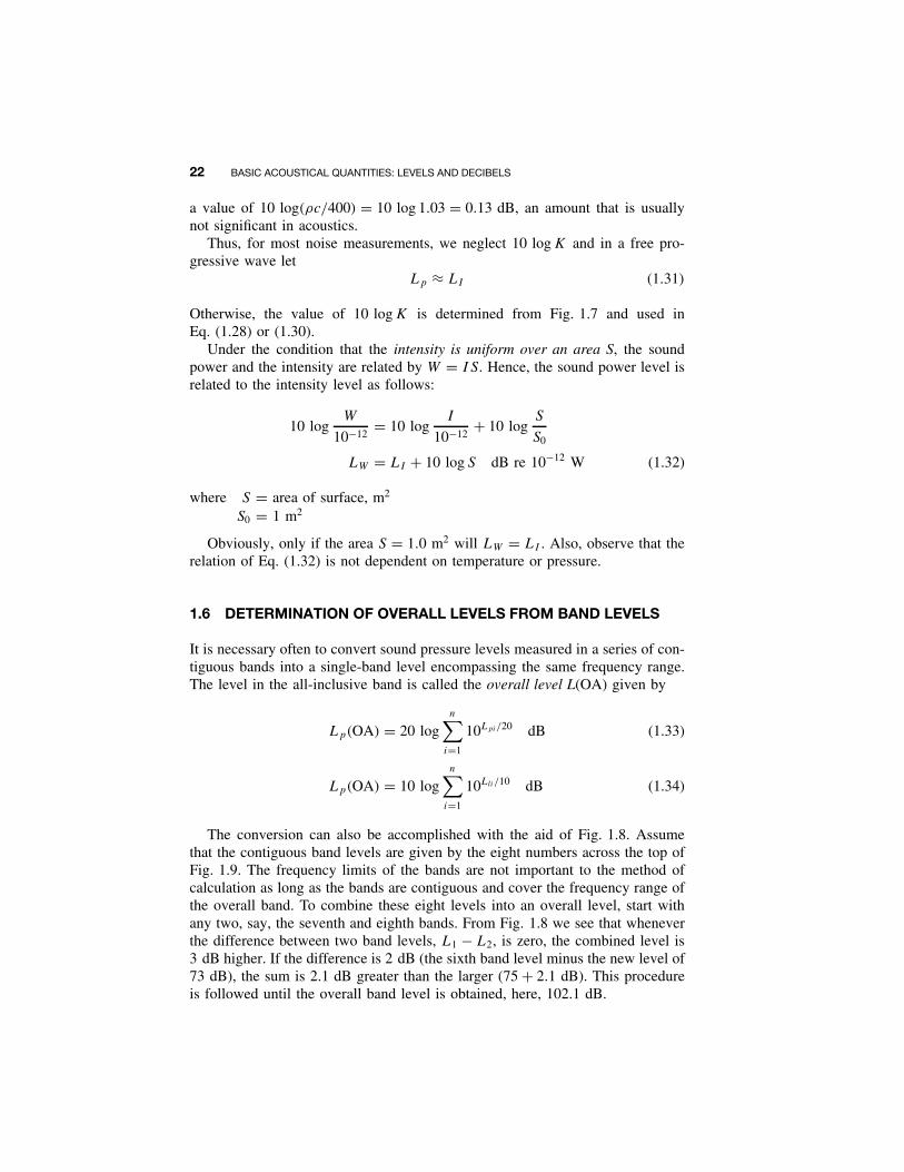
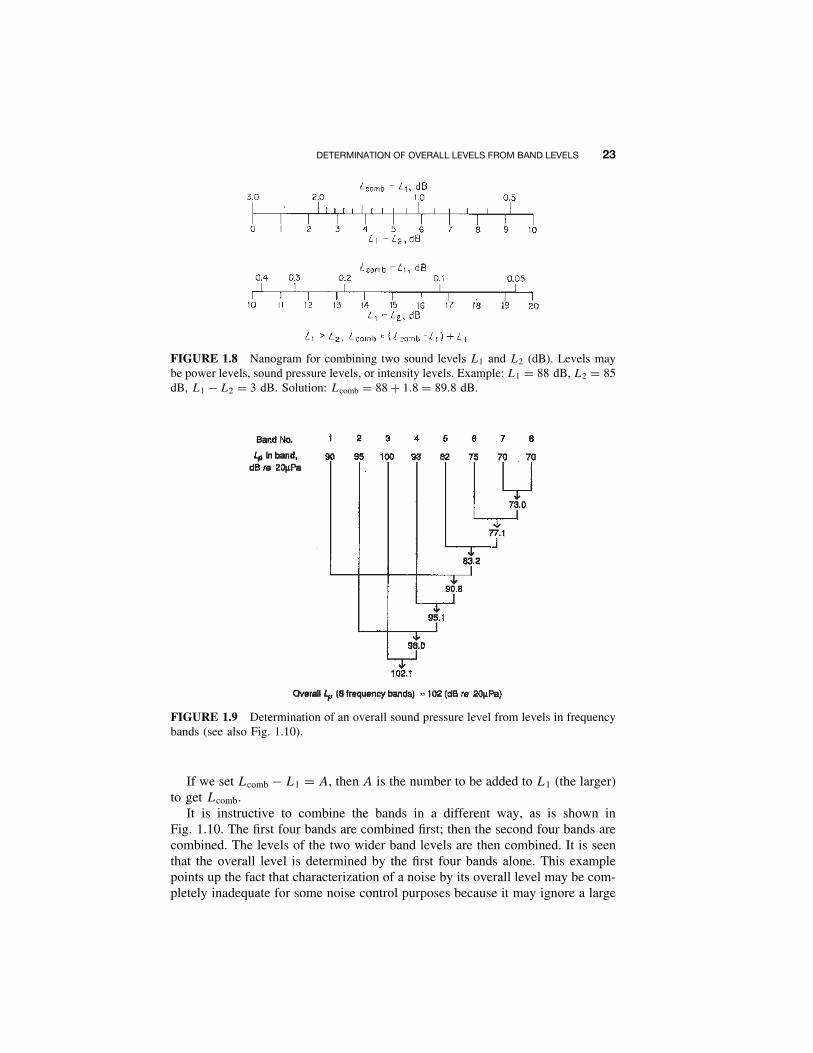
The conversion can also be accomplished with the aid of Fig. 1.8. Assumethat the contiguous band levels are given by the eight numbers across the top ofFig. 1.9. The frequency limits of the bands are not important to the method ofcalculation as long as the bands are contiguous and cover the frequency range ofthe overall band. To combine these eight levels into an overall level, start withany two, say, the seventh and eighth bands. From Fig. 1.8 we see that wheneverthe difference between two band levels, L1 − L2, is zero, the combined level is3 dB higher. If the difference is 2 dB (the sixth band level minus the new level of73 dB), the sum is 2.1 dB greater than the larger (75 + 2.1 dB). This procedureis followed until the overall band level is obtained, here, 102.1 dB.

DETERMINATION OF OVERALL LEVELS FROM BAND LEVELS 23

FIGURE 1.8 Nanogram for combining two sound levels L1 and L2 (dB). Levels maybe power levels, sound pressure levels, or intensity levels. Example: L1 = 88 dB, L2 = 85dB, L1 − L2 = 3 dB. Solution: Lcomb = 88 + 1.8 = 89.8 dB.

FIGURE 1.9 Determination of an overall sound pressure level from levels in frequencybands (see also Fig. 1.10).

If we set Lcomb − L1 = A, then A is the number to be added to L1 (the larger)to get Lcomb.

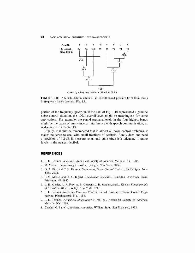
It is instructive to combine the bands in a different way, as is shown inFig. 1.10. The first four bands are combined first; then the second four bands arecombined. The levels of the two wider band levels are then combined. It is seenthat the overall level is determined by the first four bands alone. This examplepoints up the fact that characterization of a noise by its overall level may be com-pletely inadequate for some noise control purposes because it may ignore a large


FIGURE 1.10 Alternate determination of an overall sound pressure level from levelsin frequency bands (see also Fig. 1.9).

portion of the frequency spectrum. If the data of Fig. 1.10 represented a genuinenoise control situation, the 102.1 overall level might be meaningless for someapplications. For example, the sound pressure levels in the four highest bandsmight be the cause of annoyance or interference with speech communication, asis discussed in Chapter 19.

Finally, it should be remembered that in almost all noise control problems, itmakes no sense to deal with small fractions of decibels. Rarely does one needa precision of 0.2 dB in measurements, and quite often it is adequate to quotelevels to the nearest decibel.

REFERENCES

1. L. L. Beranek, Acoustics, Acoustical Society of America, Melville, NY, 1986.

2. M. Moeser, Engineering Acoustics, Springer, New York, 2004.

3. D. A. Bies and C. H. Hansen, Engineering Noise Control, 2nd ed., E&FN Spon, NewYork, 2002.

4. P. M. Morse and K. U. Ingard, Theoretical Acoustics, Princeton University Press,Princeton, NJ, 1987.

5. L. E. Kinsler, A. R. Frey, A. B. Coppens, J. B. Sanders, and L. Kinsler, Fundamentalsof Acoustics, 4th ed., Wiley, New York, 1999.

6. L. L. Beranek, Noise and Vibration Control, rev. ed., Institute of Noise Control Engi-neering, Poughkeepsie, NY, 1988.

7. L. L. Beranek, Acoustical Measurements, rev. ed., Acoustical Society of America,Melville, NY, 1988.

8. Charles M. Salter Associates, Acoustics, William Stout, San Francisco, 1998.

bernek noise control

Documents