BEST LINEAR UNBIASED PREDICTION OF PERFORMANCE AND BREEDING VALUE

C. R. Henderson, Cornell University and the University of Illinois

Introduction

Genetic progress in traits of economic importance has been im-

pressive during the past few decades. This has been due to a combina-

tion of (1) selection, primarily on additive genetic merit, (2) changes

in breed structure, and (3) crossbreeding; the relative importance

of these factors varying from species to species. This paper is

concerned with the first of these factors and is restricted to linear

models and approximate normality of distributions. It should be

understood that a linear model can include dominance and epistasis

and also interaction between genotypes and environments. This paper

presents methods for predicting both performance and breeding value.

This is a somewhat arbitrary dichotomy since breeding values are

defined in terms of average performance of progeny, and prediction

of breeding values requires performance records.

Assuming linearity, the mixed model method for best linear un-

biased prediction (BLUP) provides a powerful and flexible tool for

predictions that have very desirable properties.

I. In the class of linear, translation invariant functions

of records, the variances of errors of prediction are smaller

than any other such predictor, least-squares or selection

index for example.

2. The corelations between predictors and predictands are larger

than for any other predictor.

172

I

3. The probabilityof selectingthe better of any pair of candi-

dates for selectionis maximized (Henderson,1963).

4. If a fixed number of individualsis selectedfrom a fixed

number of candidates,the expected mean of the breeding

values of the selected individualsis maximized (Bulmer,

]980; Goffinet, 1983; Fernandoand Gianola, 1984).

These desirablepropertiesof BLUP would seem to provide compelling

reason for utilizingthe technique,provided,of course, that it

is computableat reasonablecost. Some computationalstrategies

are listed at the end of this paper.

If the model is not linear,nonlinearmethods are required,

but often linear approximationsare quite satisfactory. See Gianola

and Foulley (]983) for a good discussionof such methods.

Se|ectionIndex

Selection index has been used widely for many years. Since

BLUP is closely relatedto it, selectionindex is described in this

sectioneven though there is littlejustificationfor its use since

BLUP is no more difficult,and in some cases is easier to compute.

A linearmodel appropriatefor both selection index and BLUP is the

following.

y = XB + Zu + e. [l]

y is an n x I vector of recordsto use in the predictions.

E(y) = XB, where X is a known matrix, and B is a fixed vector

assumed known in selection index,but not in BLUP. u is a random

vector with null means and variance-covariancematrix = G. The vector,

u, includes breeding values,performance,etc.

.173

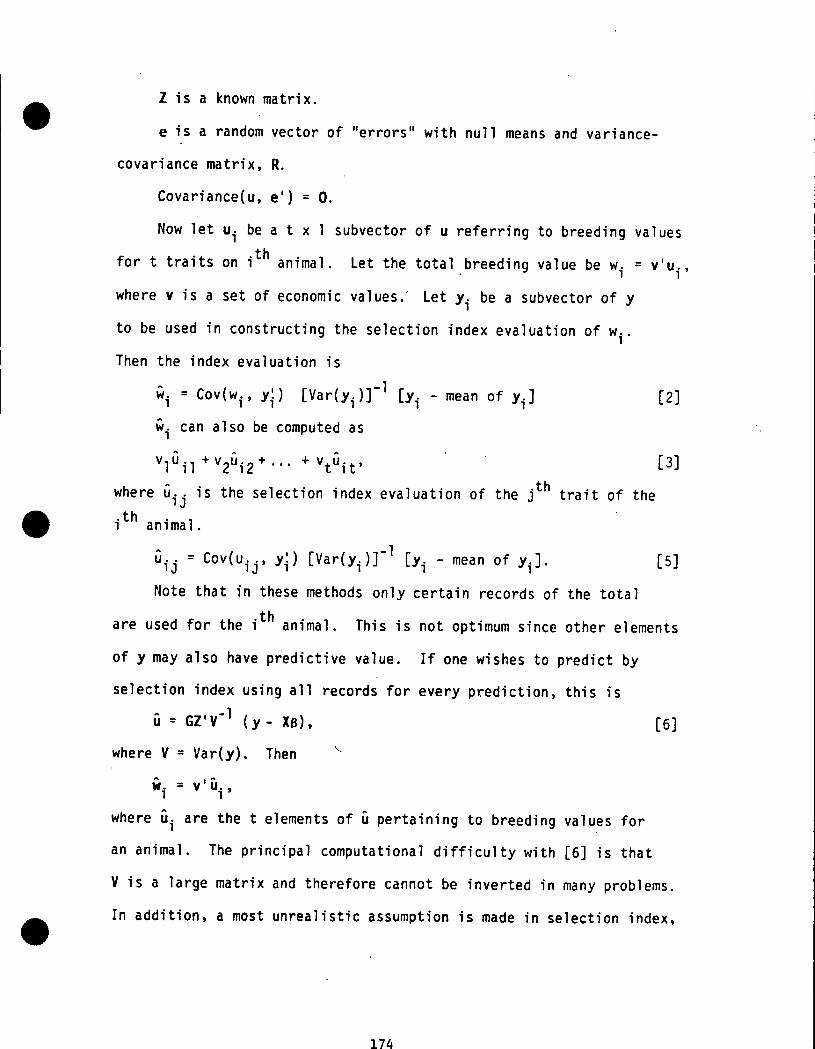
Z is a known matrix.

e is a random vector of "errors" with null means and variance-

covariance matrix, R.

Covariance(u, e') = O.

Now let ui be a t x I subvector of u referring to breeding values

for t traits on ith animal. Let the total breeding value be wi = v'u.• I'

where v is a set of economic values Let Yi be a subvector of y

to be used in constructing the selection index evaluation of wi.

Then the index evaluation is

wi = C°v(wi' Yi) [Var(Yi)]-l [Yi - mean of yi] [2]

_i can also be computed as

VlUil +v2ui2+... + vtuit, [3]

where uij is the selection index evaluation of the jthtrait of the

.th1 animal.

uij = C°v(uij' Yi)[gar(Yi)]-I [Yi - mean of yi]. [5]

Note that in these methods only certain records of the total

are used for the ith animal. This is not optimum since other elements

of y may also have predictive value. If one wishes to predict by

selection index using all records for every prediction, this is

= GZ'V-I (y- XB), [6]

where V = Var(y). Then \

wi = v'ui'

where ui are the t elements of u pertaining to breeding values for

an animal. The principal computational difficulty with [6] is that

V is a large matrix and therefore cannot be inverted in many problems.

In addition, a most unrealistic assumption is made in selection index,

174

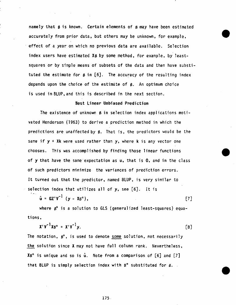
namely that B is known. Certain elements of B may have been estimated

accurately from prior data, but others may be unknown,for example,'i

effect of a year on which no previous data are available. Selection

index users have estimatedXB by some method, for example, by least-

squares or by simplemeans of subsetsof the data and then have substi-

tuted the estimatefor B in [6]. The accuracy of the resultingindex

depends upon the choice of the estimate of B. An optimumchoice

is used inBLUP,and this is described in the next section.

Best Linear Unbiased Prediction

The existenceof unknown B in selectionindex applicationsmoti-

vated Henderson (1963)to derive a predictionmethod in which the

predictionsare unaffectedby B. That is, the predictorswould be the

same if y + Xk were used rather than y, where k is any vector one

chooses. This was accomplishedby finding those linear functions

of y that have the same expectationas u, that is O, and in the class

of such predictorsminimize the variancesof predictionerrors.

It turned out that the predictor,named BLUP, is very similarto

selection index that utilizesall of y, see [6]. It is

= GZ'V"l (y- XB°), [7]

where B° is a solutionto GLS {generalizedleast-squares}equa-

tions,

X'V'IxB° = X'V-ly. [8]

The notation, B°, is used to denote some solution, not necessarily

the solution since X may not have full column rank. Nevertheless,

XB° is unique and so is G. Note from a comparison of [6] and [7]

that BLUP is simply selectionindex with B° substitutedfor B.

175•

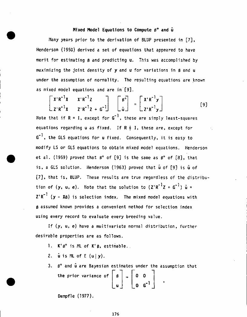
Mixed Model Equations to Compute B° and

Many years prior to the derivation of BLUP presentedin [7],

Henderson(1950)deriveda set of equations that appeared to have

merit for estimatingB and predictingu. This was accomplishedby

maximizing the joint density of y and u for variationsin B and u

under the assumptionof normality. The resultingequationsare known

as mixed model equationsand are in[9].

= [g]LZ'R'Ix Z'R'Iz + G- Z'R-ly

Note that if R = I, except for G-l, these are simply least-squares

equationsregardingu as fixed. If R + I, these are, except for -

G-l, the GLS equationsfor u fixed. Consequently,it is easy to

modify LS or GLS equationsto obtain mixed model equations. Henderson

et al. (1959)proved that B° of [9] is the same as B° of [8], that

is, a GLS solution. Henderson (1963) proved that u of [9] is u of

[7], that is, BLUP. These resultsare true regardlessof the distribu-

tion of (y, u, e). Note that the solutionto (Z'R-Iz+ G-l) _ =

Z'R-l (y - XB) is selectionindex..The mixed model equationswith

B assumed known providesa convenientmethod for selectionindex

using every recordto evaluate every breeding value.

If (y, u, e) have a multivariatenormal distribution,further

desirablepropertiesare as follows.

I. K'B° is ML of K'B, estimable.

2. _ is ML of E (uly).

3. B° and u are Bayesian estimatesunder the assumptionthat

[:][ ithe prior variance of _ 0 0

0 G-l

Dempfle(1977).

176

It appears,therefore,that if a linear model and approximate

normalitycan be invoked,BLUP should be used as the selectioncri-

terion provided it can be computed. Certainly [9] is usuallyeasier

to computethan [7]. First, R-l is ordinarilymuch easier than V-l

even though they have the same dimension. R usually has some simple

form such as Io_ or is block diagonal. Similarly,G-l is often simple,

and, in particular,when G = Ao_- sihce A"l can be computed very rapidly

with no need for A (Henderson,1976). Finally, the coefficientmatrix

and particularlythe u part usuallyexhibits diagonal or block diagonal

dominancetherebyresultingin equationswell suited to iterative

solution. Animal breeders, particularlyat Guelph and Cornell, have

been successfullysolving very large sets of equationsfor dairy

sire and cow evaluationsby BLUP.

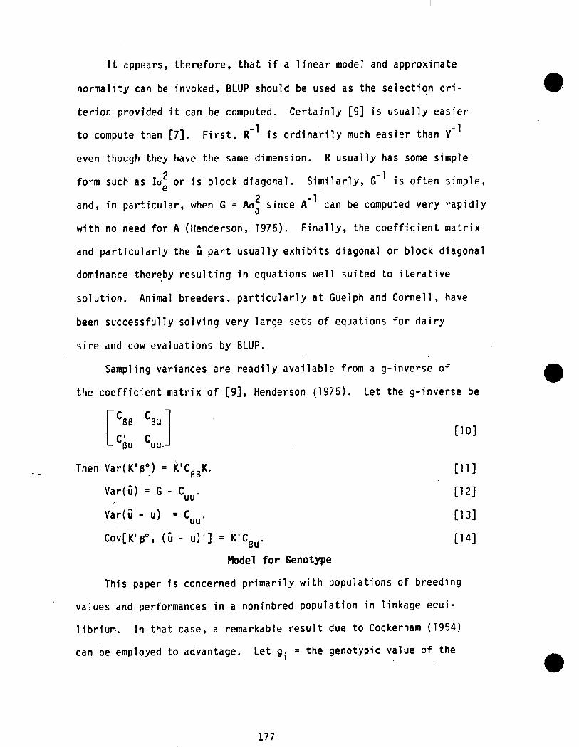
Samplingvariancesare readily availablefrom a g-inverseof

the coefficientmatrix of [9], Henderson (1975). Let the g-inverse be

[CBB CBu_ [lO]CuuJ

Then Var(K'B°) '._ : KC BK. Ill]

Var(_) = G - Cuu. [12]

Var(_ - u) = Cuu. [13]

Cov[K'B°, (u- u)'] : K'CBu. [14]

_del for _notype

This paper is concerned primarilywith populationsof breeding

• values and perfomances in a noninbredpopulation in linkageequi-

librium. In that case, a remarkableresult due to Cockerham (1954)

can be employed to advantage. Let gi = the genotypicvalue of the

177II

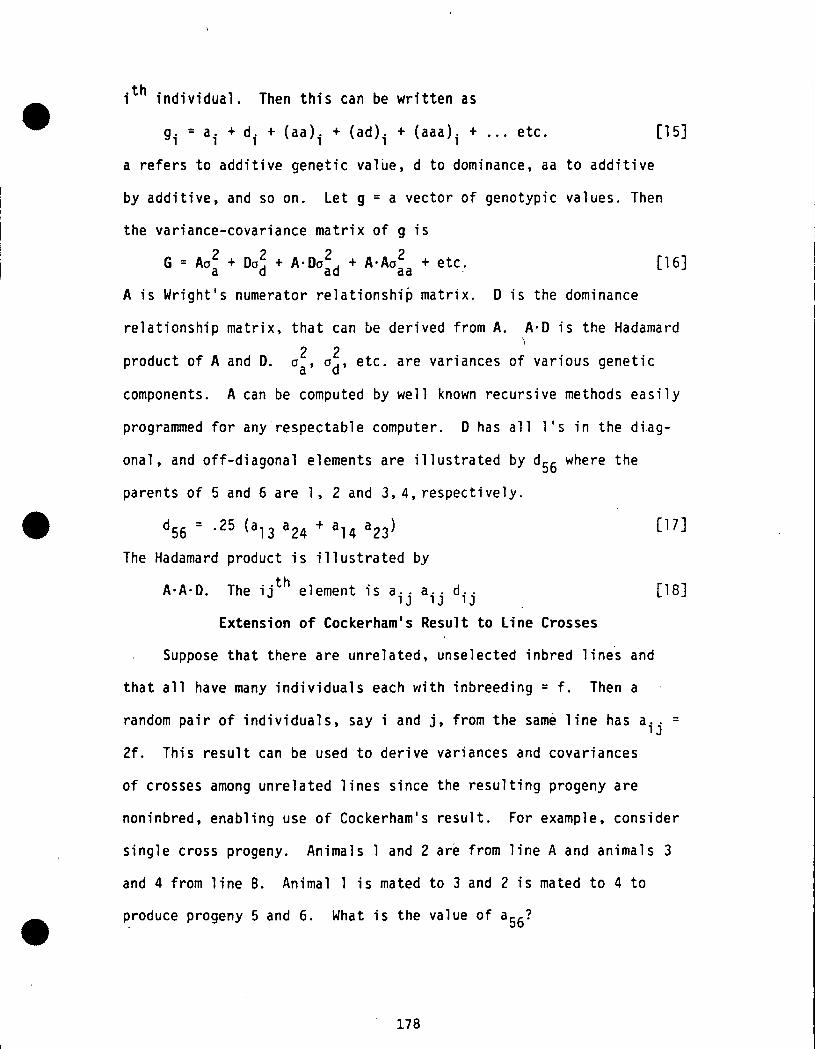
ith individual. Then this can be written as

gi = ai + di + (aa)i + (ad)i + (aaa)i + "'" etc. [15]

a refers to additive genetic value, d to dominance, aa to additive

by additive, and so on. Let g = a vector of genotypic values. Then

the variance-covariance matrix of g is

G = Ao_ . Da_ + A.Da_d . A.A_a .etc. [163

A is Wright's numerator relationship matrix. D is the dominance

relationship matrix, that can be derived from A. A.D is the Hadamard

2 2product of A and D. _a' Od' etc. are variances of various genetic

components. A can be computed by well known recursive methods easily

programmed for any respectable computer. D has all l's in the diag-

onal, and off-diagonal elements are illustrated by d56 where the

parents of 5 and 6 are l, 2 and 3, 4, respectively.

d56 = .25 (al3 a24 + al4 a23) [17]

The Hadamard product is illustrated by

A.A.D. The ijth element is aij aij dij [18]

Extension of Cockerham's Result to Line Crosses

Suppose that there are unrelated, unselected inbred lines and

that all have many individuals each with inbreeding = f. Then a

random pair of individuals, say i and j, from the same line has aij =

2f. This result can be used to derive variances and covariances

of crosses among unre]ated lines since the resulting progeny are

noninbred, enabling use of Cockerham's result. For example, consider

single cross progeny. Animals l and 2 are from line A and animals 3

and 4 from line B. Animal l is mated to 3 and 2 is mated to 4 to

produce progeny 5 and 6. What is the value of a56?

178

2f J• 2

_ 3---_ 62f 174

Then by path coefficientmethodology,a56 = .25(2f)+ .25(2f)= f

d56 = .25(2f.2f+ 0.0) = f2.

Then (ad)56= f.f2 = f3.

(aa)56= f.f = f2.

etc.

But since the varianceof-a line cross is the covariancebetween

any pair of individualsfrom that cross, the varianceof single cross

means is

2 2 f3 2 + etc / [19]fo_ + f2o + f Oaa + Oad

Note that when f = |, this is the same as the varianceof individual

genotypesin the population from which the lines were derived. By

the same principles,the variance of 3-way crosses and 4-way cresses are

.75 f 2 + 5 f2od2+ 9 2 + 3 2 + etc. [20]°a " T6 °aa 8 °ad '

l 2 l 22 +__ 32and _ fOa +_ f2o2 +_ f Oaa f Oad + ..respectively. [21]

BLUP of PerformanceRecordson One Trait

Let the model for recordson a single trait be

y = XB + ZlW + Z2g + e [22]

XB is the fixed mean of y,

w is a random vector of effectsother than g,

g is a vector of random genotypicvalues,and

e is the error vector.

179

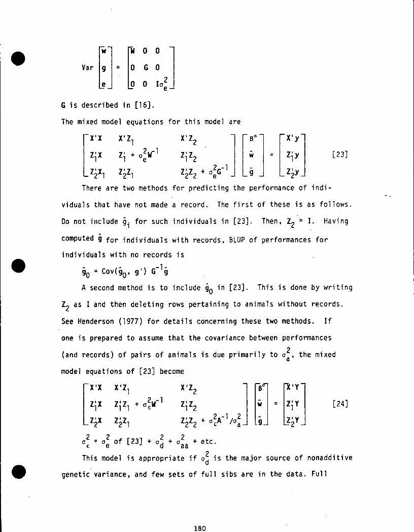
E°°]Var = G 0

O Ioe2

G is describedin [16].

The mixed model equations for this model are

l'l X'Z1 X'Z2 X'y

LZ_XI z_z_ z_z2+o_G"l z_yThere are two methods for predicting the performance of indi-

viduals that have not made a record. The first of these is as follows.

Do not include gi for such individuals in [23]. Then, Z2 : I. Having

computed g for individuals with records, BLUPof performances for

individuals with no records is

go=c°v(go'g')G-Ig

A secondmethod is to includego in [23]. This is done by writing

Z2 as I and then deleting rows pertainingto animals without records.

See Henderson(1977) for details concerningthese two methods. If

one is prepared to assume that the covariancebetween performances

(and records)of pairs of animals is due primarilyto 02 the mixeda'

model equationsof [23] become

zlxzlz+o w zlz2 : lZiY2 -LZ_yLZ_X Z_Z1 Z_Z2 + o2EA"I/oa

ac °aa

This model is appropriate if o2 is the major source of nonadditive

genetic variance, and few sets of full sibs are in the data. Full

180

sibs are the only relatives in noninbredpopulationswith appreciable

2_d in their covariance. The advantageof [24] over [23] computa-

tionally is that the rapid method for computingA"l can be used.

Meaning of BreedingValues of Individuals

The breedingva]ue (b.v.)of an individualis the mean performance

of many progeny resultingfrom matingswith a large random sample

fromaspecifiedpopulation. Note that b.v. has no meaning uniess

the populationof mates is defined. If a longer view is taken, b.v.

could be definedas the mean performanceof descendants_ generations

removed. Under the first definition,the covariancebetween parental

genotype and progeny performanceis

.5o_ + .25_a + .125O_aa+ ... [25]

Note that dominancedoes not contributeto covariance. If the second

definitionis used, the covariance is

-n 2 2-2no2 -3n 22 oa + + 2 + [26]aa °aaa "'"2a dominatesthis covariance. Consequently,apart from thea

sca]ar 2-n, additive genetic value and breeding value are almost

the same. This must be the reason why breeders generally use the

terms breedingvalue and additive geneticvalue interchangeably. Under

this assumption,a can be predictedfrom [24] and then the predictionil

of theperformance of a random progenyof an individual is .5_.

A Possib|y More Accurate Method for Breeding Values

If one is not prepared to accept a = b.v., one can solve equation

[23] for g and from this predict,a, aa, etc. These are simp|e.

2 -i= aaAG g,

2 (A.A) G'I_,aa : Caa

181.

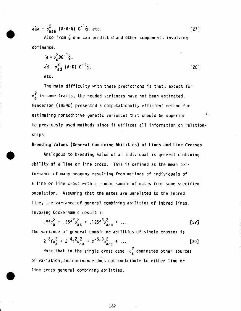
a_a = Oaaa2 (A.A.A)G-l_, etc. [27]

Also from g one can predictd and other components involving

dominance.

"_ = o_DG-I_,2

id = aad (A.D) G-l_, [28]

etc.

The main difficulty with these predictionsis that, except for

2aa in some traits, the needed varianceshave not been estimated.

Henderson (1984b) presenteda computationallyefficientmethod for

estimatingnonadditivegenetic variancesthat should be superior "-

to previously used methods since it utilizesall informationon relation-

ships.

Breeding Values (GeneralCombiningAbilities)of Lines and Line Crosses

Analogous to breeding value of an individualis general combining

ability of a line or line cross. This is defined as the mean per-

formanceof many progeny resultingfrom matingsof individualsof

a line or line cross with a randomsample of mates from some specified

population. Assuming that the mates are unrelatedto the inbred

line, the variance of general combiningabilitiesof inbred lines,

invokingCockerham'sresult is

22 32.5fa_ + .25f aaa + .125f aaaa + ... [29]

The varianceof general combiningabilitiesof single crosses is

-2 2 4_2 2 _-6_3 22 faa + 2- T aaa + _ T aaaa + ... [30]

single cross case, o_ dominatesother sourcesNote that in the

of variation,and dominance does not contributeto either line or

line cross general combining abilities.

182

Specific BreedingValue

Specific breeding value has meaning only in the context of a

pair of mates. It is defined as the mean performance of many progeny

of a specific mating. If the genetic model contains important non-

additive genetic components, prediction of the specific breeding

Value with appreciablelaccuracy requires a large set of full-sib

progeny. In the absence of such progeny, the prediction of the spe-

cific value of i mated with j is essentially

.5(_i + _j) + .25(_ai + aaj) + .125(aaai + aaaj) + ... [31].

That is, no contributionof dominanceto specific breeding value

is present. In contrast, if full-sibprogeny are available, the

predictionis some function like [31] plus some linear function of

the predicteddominancevalues of these full sibs.

Specific breeding values of cattle and sheep are obtained largely

from predictionsof the additivevalues of the two mates, since few

full-sib sets are available for prediction. Pigs, of course, provide

substantialnumbersof full-sib sets, but these are usually litter-

mates, and consequentlyspecificbreeding values and maternal effects

are seriouslyconfounded. Poultrycertainlyprovide the greatest

opportunityfor capitalizingon specificbreeding va]ues.

Specific CombiningAbilitiesof Line Crosses

Maximum utilizationof nonadditivegenetic variance requires

testingof crosses among highly inbred lines. Equations [19];,[20]

and [2l] emphasize two importantaspectsof line crossing. First,

high levels of inbreedingare requiredsince the contributionof

_ nonadditivecomponents to linecross differencesare functionsof

183iiI

powers of f. Thus, the contribution of high order interactions rises

almost exponentially with increases in inbreeding. Second, single

cross differences contain much larger functions of nonadditive variance

than three-way crosses, and the latter more than four-way crosses.

It is not surprising that single cross hybrids have become increasingly

used in corn production. It is doubtful if the technique is useful

in large animal breeding considering the cost of producing, testing,

and maintaining highly inbred lines.

Multiple Trait Evaluation

Two general methods have been used for prediction of breeding

values of correlated traits; first, sire evaluation, and second,

individual animal evaluation under the animal model (AM) described

thbelow. Let the AM for the set of records on the i trait be Yi

= XiBi + Ziai + ei (i = l, ... , t) [32]

Then if breeding values are ordered animals in traits and all are

included regardless of whether there is a record,

I!]rVar " [33]

LAgit Agtt

The gij are variances and covariances in the t x t genetic covariance

matrix for a noninbred, unselected population. If all traits are

observed on all animals and records are ordered animals within traits,

[i!IE!Var = " [34]

it "'" Irtt

184

The rij are elements of the usual environmentalcovariancematrix.

Thus hi2= gii/(gii + rii)' geneticcorrelationbetween i and j traits

= gij/(giigjj) "5, and phenotypic correlation = (gij + rij)/(gii +

rii)'5(gjj+ rjj)"5 Then if we includeall elements of a in the

mixed model equations, the inverseof G needed is simply

A'IgII ... A'IgIt]

G'l= " " [35]

[A-lglt ... A-lgtt

A-l is easy to compute and the gij are elements of the inverse

of the t x t genetic variance-covariancematrix. If all records

are present,

rll "'" irltl

R'I: " " [36]

r It ... Ir tt

If recordsare missing, it is easier computationallyto order

the data traits in animals. Then R and R°l are block diagonalmatrices

with the block for the ith animal having order equal to the number

of traits recordedon that animal. Using these ideas, Henderson

and Quass (1976)described in detail multiple trait BLUP evaluationI

for the animal model.

Maternal Effects

Maternal effects can be includedeasily in mixed model equations,

for exampleQuaas and Pollak (1980). The principaldifficultywith

this is that good estimatesof maternal variances are available for

few, if any, traits. Some of the newer methods for variance estimation

show promise for estimatingthese variancesas well as additiveand

185

nonadditivegeneticvariances. ProbablyMIVQUE, REML or ML are the

methods of choice. See Henderson(1984a)for detailsof the methods

and for numericalexamples.

The Problemof SelectionBias

The precedingsectionsassume that the varianceof additive

genetic values is Ao_ and breeding values,a, areuncorrelatedwith

the error vector that is assumed to have variance,la_ for a single

trait. Also, it is assumed that the mean of a is null. Now if selec-

tion has been practicedand it has been effective,these assumptions- °

quite clearly are not true. The breeding values in later generations

will have means greaterthan O. Further, it is well known that selec-

tion tends to reduce genetic varianceand to alter geneticcorrela-

tions. It is not correct to assume that after selectionthe variance

of a is A times the new genetic variance. The A matrix is also al-

tered. In fact, unrelatedanimals can have nonzero correlations

between their breedingvalues. To furthercomplicatethe situation,

nonzero covariancesbetweena and e can be generated. It has sometimes

been suggestedthat geneticparametersshould be re-estimatedper-

iodicallyand these new estimates used in predictionfrom later data.

From the foregoingit can be seen that this is not a sufficienttool

because ofalterationof A and presenceof covariancesbetween a and

e. Fortunately,there is a simple solutionto this seeminglyintract-

able problem. Henderson(1975) proved that if the followingconditions

hold, mixed mode] equationswritten as if no selectionhad occurred

and using parametervalues existing before selectionbegan yields

BLUE and BLUP under the selectionmodel that has alteredVar(u'_e')

186

and the means.

I. Multivariatenormal distribution.

2. Selectiondecisionsbased on linear, translationinvariant

functionsof the records.

3. G and R prior to selectionknown at least to proportionality.

4. All data used in the mixed model equations, includingdata

used both to select anima]sand to reject animals.

This method for dealing with the selectionproblem requires

that we have good estimatesof the base population G and R. Is this

possiblewhen the data availablefor estimation have arisen from

a selectionprogram? It appearsthat REML applied to data that meet

the requirements], 2 and 4 for prediction listed above yields esti-

mates of the base populationparametersthat are not biased by.selec-

tion.

Some ComputingProblemsand Possible So]utions

It is obvious that a multiple trait evaluationof a large number

of animalsby BLUP requires the solution to a very large set of equa-

tions. In most cases, these cannot be solved by the conventional ° _

reductionmethod since for efficientcomputing the coefficientmatrix

needs to be stored in core. Fortunately,however, iterativemethods

for solutionusuallywork very well. In single trait problems the

coefficientmatrix pertainingto a has large diagonal elements as

compared to off-diagonal. Consequently,Gauss-Seide]iterationworks

well. With this method, it is easy to retrieve the coefficientmatrix

from auxiliarystorage. Also coefficientsthat are 0 need not be

stored. At Cornell we solve a set of equations involvingapproximately

187

ii

7,000 sires, after absorbing many tens of thousands of equations

for herd-year-seasons, in about 15 minutes. As evaluations proceed

from one year to another, one can use to advantage starting values

for iteration that were the converged values in the previous run

for those animals that continue on the system.

For multiple trait problems it is desirable to order the a vector

by traits within anima]s. Then the mixed model coefficient matrix

exhibits blocks of coefficients down the diagonal that dominate the

other coefficients. Thus, at any round, the solution for the breeding

values for the ith-_nimal is

1Bi r i ,

where Bi is the block of coefficients of order equal to the number

of traits and _ is the corresponding right hand sides adjusted for

the current solutions for the other animals. Of course, the Bilremains

fixed and these can be computed at the start of iteration and stored

for subsequent use.

Quaas and Pollak (1980) have described a reduced animal model

(RAM) that can markedly reduce the number of equations. By this

method, the only breeding values included in the equations are those

of animals that have one or more progeny with records. After solving

for the breeding values of these parents, the breeding values of

the progeny are predicted by a back solution. Henderson (1984)

has developed MIVQUE and REML algorithms for estimation of additive

genetic and error variances using these reduced sets of equations.

This should enable estimation of additive genetic variance from large

data sets and taking advantage of the power of the A matrix to control

188

on selectionbias.

Anotherdevelopmentthat should eliminate some of the pessimism

concerningcomputingproblems is the spectacularlyrapid improvement

in the speed and memory size of computers. We are now carrying out

computationsthat would have been consideredimpossiblea few years

ago. Some computerexperts regard the industryas still being in

its infancy.

189

LiteratureCited

Bulmer, M. G. 1980. The _|athematicalTheory of QuantitativeGenetics.

Oxford Univ. Press.

Cockerham,C. C. 1954. An extensionof the conceptof partitioning

hereditaryvariance for analysis of covariancesamong relatives

when epistasisis present. Genetics39:859.

Dempfle, L. 1977. Relation entre BLUP (Best Linear Unbiased Pre-

diction)et estimateursBayesians. Ann. Genet. Sel. Anim. 9"27.

Fernando,R. L. and D. Gianola. 1984. Optimum rules for selection.

Mimeo, Dept. of Animal Science,Univ. of Illinois.

" Gianola,D. and J. L. Foulley. 1983. New techniquesof prediction

of breeding value for discontinuoustraits. 32nd Annu. Natl.

BreedersRoundtable.

Goffinet,B. ]983. Selection on selectedrecords. Genet. Sel.

Eval. 15:91.

Henderson,C. R. 1950. Estimationof geneticparameters. Ann.

Math. Star. 21:309.

Henderson,C. R. 1963. Selectionindex and expected genetic advance.

NAS-NRC Publ. 982.

Henderson,C. R. 1975. Best ]inear unbiasedestimationand prediction

under a selectionmodel. Biometrics31:423.

Henderson,C. R. 1976. A simp|e method for computingthe inverse

of a numeratorrelationshipmatrix used in predictionof breeding

values. Biometrics32:69.

Henderson,C. R. 1977. Best linear unbiasedpredictionof breeding

values not in the model for records. J. Dairy Sci. 60:783.

190

Henderson,C. R. 1984a. Applicationsof Linear _Iodeisin Animali

Breeding. Univ. of Guelph (in press).

Henderson,C. R. 1984b. Best linear unbiased predictionof non-

additive geneticmerits in noninbredpopulations. J. Anim.

Sci. (in press).

Henderson,C. R., O. Kempthorne,S. R. Searle and C. M. von Krosigk.

1959. The estimationof environmentaland genetictrends from

recordssubject to culling. Biometrics15:192.

Henderson,C. R. and R. L. Quaas. 1976. _ultipIe trait evaluation

using relatives'records. J. Anim. Sci. 43:1188.

Quaas, R. L. and E. J. Pollak. 1980. Mixed mode] methodologyfor

farm and ranch beef cattle testing programs. J. Anim. Sci.

51:1277.

M2:0027984

191

BEST LINEAR UNBIASED PREDICTION OF PERFORMANCE AND BREEDING VALUE

Questions and Answers

i. Alan Emsley

What is the potential improvement in accuracy from BLUP over least squares etc?

C.R. Henderson

The principal alternatives to BLUP are least squares, regressed least squares,and selection index. All of these have similarities, but in the case of linear,

unbiased predictions BLUP is always more accurate, how much more depends upon

the data set and upon the underlying parameters. Least squares and regressed

least squares are not suitable for multiple traits. In the case of single

traits, and with all candidates for selection having the same amount of infor-mation and unrelated to one another, least squares and BLUP rank animals the

same, With unequal information least squares selects too high a proportionof animal with limited information. Regressed least squares solves this problem

by regressing least squares predictions by amount inversely according to theamount of information. Regressed least squares as used in practice does not

utilize all of the information. However, an appropriate set of linear functions

of least squares predictions is, in fact, BLUP, but cumbersome to compute.

Selection index has two deficiencies, first B is assumed known even though it

never is. Consequently, it is estimated, and unless the estimate is GLS, the

resulting predictions are less accurate than BLUP. Consequently, selection

index as compared to BLUP depends upon how B is estimated. Also in practice,

selection index, in contrast t_ BLUP, does not use all information. If onewanted to do this, adjust the u equation of [92 for the estimate of B and

• _

then solve.

As described in my paper, BLUP has optimum properties for selection and is as

easy to compute as alternatives. Consequently, why use anything else?-i ^

(Z'R Z+G) u = ZjR-l(y-X_).2. John Keele _ _ N_ _ _ _ _ _

How does one incorporate genotype x environmental interaction into BLUP?

Genotype x environmental interaciton is easy to incorporate. Include in the

model a vector, say_y, referring to this interaction. We would usually assume

t_at it has variance _y. Therefore we would add i/4_to the diagonals of thesubmatrix of coefficients in equations [23] a_gmented for this factor.

Since this submatrix is diagnoal, absorption of y is easy.

192