best subset selection via a modern optimization lensdbertsim/papers/machine learning under a...
TRANSCRIPT

The Annals of Statistics2016, Vol. 44, No. 2, 813–852DOI: 10.1214/15-AOS1388© Institute of Mathematical Statistics, 2016
BEST SUBSET SELECTION VIA A MODERNOPTIMIZATION LENS
BY DIMITRIS BERTSIMAS, ANGELA KING AND
RAHUL MAZUMDER1
Massachusetts Institute of Technology
In the period 1991–2015, algorithmic advances in Mixed Integer Opti-mization (MIO) coupled with hardware improvements have resulted in anastonishing 450 billion factor speedup in solving MIO problems. We presenta MIO approach for solving the classical best subset selection problem ofchoosing k out of p features in linear regression given n observations. Wedevelop a discrete extension of modern first-order continuous optimizationmethods to find high quality feasible solutions that we use as warm starts to aMIO solver that finds provably optimal solutions. The resulting algorithm (a)provides a solution with a guarantee on its suboptimality even if we terminatethe algorithm early, (b) can accommodate side constraints on the coefficientsof the linear regression and (c) extends to finding best subset solutions for theleast absolute deviation loss function. Using a wide variety of synthetic andreal datasets, we demonstrate that our approach solves problems with n inthe 1000s and p in the 100s in minutes to provable optimality, and finds nearoptimal solutions for n in the 100s and p in the 1000s in minutes. We alsoestablish via numerical experiments that the MIO approach performs betterthan Lasso and other popularly used sparse learning procedures, in terms ofachieving sparse solutions with good predictive power.
1. Introduction. We consider the linear regression model with response vec-tor yn×1, model matrix X = [x1, . . . ,xp] ∈ R
n×p , regression coefficients β ∈ Rp×1
and errors ε ∈ Rn×1: y = Xβ + ε. We will assume that the columns of X have
been standardized to have zero means and unit �2-norm. In many important clas-sical and modern statistical applications, it is desirable to obtain a parsimoniousfit to the data by finding the best k-feature fit to the response y. Especially in thehigh-dimensional regime with p � n, in order to conduct statistically meaningfulinference, it is desirable to assume that the true regression coefficient β is sparse.Quite naturally, the last few decades have seen a flurry of activity in estimating
Received June 2014; revised August 2015.1Supported by ONR-N00014-15-1-2342 and an Interface grant from the Moore Sloan Foundation.MSC2010 subject classifications. Primary 62J05, 62J07, 62G35; secondary 90C11, 90C26,
90C27.Key words and phrases. Sparse linear regression, best subset selection, �0-constrained minimiza-
tion, lasso, least absolute deviation, algorithms, mixed integer programming, global optimization,discrete optimization.
813

814 D. BERTSIMAS, A. KING AND R. MAZUMDER
sparse linear models with good explanatory power. Central to this statistical tasklies the best subset problem [Miller (2002)] with subset size k, which is given bythe following optimization problem:
minβ
1
2‖y − Xβ‖2
2 subject to ‖β‖0 ≤ k,(1.1)
where the �0 (pseudo)norm of a vector β counts the number of nonzeros in βand is given by ‖β‖0 = ∑p
i=1 1(βi �= 0), where 1(·) denotes the indicator func-tion. The cardinality constraint makes problem (1.1) NP-hard [Natarajan (1995)].Indeed, state-of-the-art algorithms to solve problem (1.1), as implemented in popu-lar statistical packages, like leaps in R, do not scale to problem sizes larger thanp = 30. Due to this reason, it is not surprising that the best subset problem hasbeen widely dismissed as being intractable by the greater statistical community.
In this paper, we address problem (1.1) using modern optimization methods,specifically mixed integer optimization (MIO) and a discrete extension of first-order continuous optimization methods. Using a wide variety of synthetic and realdatasets, we demonstrate that our approach solves problems with n in the 1000sand p in the 100s in minutes to provable optimality, and finds near optimal solu-tions for n in the 100s and p in the 1000s in minutes. To the best of our knowledge,this is the first time that MIO has been demonstrated to be a tractable solutionmethod for problem (1.1). We note that we use the term tractability not to meanthe usual polynomial solvability for problems, but rather the ability to solve prob-lems of realistic size with associated certificates of optimality, in times that areappropriate for the applications we consider.
Brief context and background. As there is a vast literature on the best sub-set problem, we present a brief and selective overview of related approaches. Toovercome the computational difficulties of the best subset problem, computation-ally friendlier convex optimization based methods like Lasso [Chen, Donoho andSaunders (1998), Tibshirani (1996)] have been proposed as a surrogate for prob-lem (1.1). For the linear regression problem, the Lagrangian form of Lasso solves
minβ
1
2‖y − Xβ‖2
2 + λ‖β‖1,(1.2)
where the �1 penalty on β , that is, ‖β‖1 = ∑i |βi | shrinks the coefficients toward
zero and produces a sparse solution by setting many coefficients to be exactly zero.There has been a substantial amount of impressive work on Lasso [Bickel, Ri-tov and Tsybakov (2009), Candès and Plan (2009), Donoho (2006), Efron et al.(2004), Greenshtein and Ritov (2004), Knight and Fu (2000), Meinshausen andBühlmann (2006), Wainwright (2009), Zhang and Huang (2008), Zhao and Yu(2006)] in terms of algorithms and understanding of its theoretical properties; seealso the excellent books or surveys [Bühlmann and van de Geer (2011), Hastie,

BEST SUBSET SELECTION VIA A MODERN OPTIMIZATION LENS 815
Tibshirani and Friedman (2009), Tibshirani (2011)]. Indeed, Lasso enjoys sev-eral attractive statistical properties. Under various conditions on the model matrixX and n,p,β , it can be shown that Lasso delivers a sparse model with goodpredictive performance [Bühlmann and van de Geer (2011), Hastie, Tibshirani andFriedman (2009)]. In order to perform exact variable selection, much stronger as-sumptions are required [Bühlmann and van de Geer (2011)]. Sufficient conditionsunder which Lasso gives a sparse model with good predictive performance arethe restricted eigenvalue conditions and compatibility conditions [Bühlmann andvan de Geer (2011)]. These involve statements about the spectrum of submatricesof X and are difficult to verify [Bandeira et al. (2013)] for a given data-matrix X.An important reason behind the popularity of Lasso is perhaps its computationalefficiency and scalability to practical sized problems. Problem (1.2) is a convexquadratic optimization problem and there are several efficient solvers for it; see,for example, Efron et al. (2004), Friedman et al. (2007), Nesterov (2013).
In spite of its favorable statistical properties, Lasso has several shortcomings.In the presence of noise and correlated variables, in order to deliver a model withgood predictive accuracy, Lasso brings in a large number of nonzero coefficients(all of which are shrunk toward zero) including noise variables. Lasso leads tobiased regression coefficient estimates, since the �1-norm penalizes the large coef-ficients more severely than the smaller coefficients. In contrast, if the best subsetselection procedure decides to include a variable in the model, it brings it in with-out any shrinkage thereby draining the effect of its correlated surrogates. Uponincreasing the degree of regularization, Lasso sets more coefficients to zero, butin the process ends up leaving out true predictors from the active set. Thus, assoon as certain sufficient regularity conditions on the data are violated, Lassobecomes suboptimal as (a) a variable selector and (b) in terms of delivering amodel with good predictive performance. The shortcomings of Lasso are alsoknown in the statistics literature. In fact, there is a significant gap between whatcan be achieved via best subset selection and Lasso: this is supported by em-pirical (for small problem sizes, i.e., p ≤ 30) and theoretical evidence; see, forexample, Greenshtein (2006), Mazumder, Friedman and Hastie (2011), Raskutti,Wainwright and Yu (2011), Shen et al. (2013), Zhang, Wainwright and Jordan(2014), Zhang and Zhang (2012) and the references therein. Some discussion isalso presented in Section 4.
To address the shortcomings, nonconvex penalized regression is often used to“bridge” the gap between the convex �1 penalty and the combinatorial �0 penalty[Candès, Wakin and Boyd (2008), Fan and Li (2001), Frank and Friedman (1993),Friedman (2008), Mazumder, Friedman and Hastie (2011), Zhang (2010a, 2010b),Zhang and Huang (2008), Zou (2006), Zou and Li (2008)]. Written in Lagrangianform, this gives rise to continuous nonconvex optimization problems of the form
1
2‖y − Xβ‖2
2 + ∑i
p(|βi |;γ ;λ)
,(1.3)

816 D. BERTSIMAS, A. KING AND R. MAZUMDER
where p(|β|;γ ;λ) is a nonconvex function in β with λ and γ denoting the degreeof regularization and nonconvexity, respectively. Typical examples of nonconvexpenalties include the minimax concave penalty (MCP), the smoothly clipped ab-solute deviation (SCAD) and �γ penalties [see, e.g., Fan and Li (2001), Frank andFriedman (1993), Mazumder, Friedman and Hastie (2011), Zou and Li (2008)].There is strong statistical evidence indicating the usefulness of estimators obtainedas minimizers of nonconvex penalized problems (1.3) over Lasso; see, for ex-ample, Fan and Lv (2011, 2013), Loh and Wainwright (2013), Lv and Fan (2009),van de Geer, Bühlmann and Zhou (2011), Zhang (2010a), Zhang and Zhang(2012), Zheng, Fan and Lv (2014). In a recent paper, Zheng, Fan and Lv (2014) dis-cuss the usefulness of nonconvex penalties over convex penalties (like Lasso) inidentifying important covariates, leading to efficient estimation strategies in highdimensions. They describe interesting connections between �0 regularized leastsquares and least squares with the hard thresholding penalty; and in the processdevelop comprehensive global properties of hard thresholding regularization interms of various metrics. Fan and Lv (2013) establish asymptotic equivalence of awide class of regularization methods in high dimensions with comprehensive sam-pling properties on both global and computable solutions. Problem (1.3) mainlyleads to a family of continuous and nonconvex optimization problems. Various ef-fective nonlinear optimization based methods [see, e.g., Candès, Wakin and Boyd(2008), Fan and Li (2001), Loh and Wainwright (2013), Mazumder, Friedman andHastie (2011), Zhang (2010a), Zou and Li (2008) and the references therein] havebeen proposed in the literature to obtain good local minimizers to problem (1.3).In particular, Mazumder, Friedman and Hastie (2011) propose Sparsenet, acoordinate-descent procedure to trace out a surface of local minimizers for prob-lem (1.3) for the MCP penalty using effective warm start procedures.
The Lagrangian version of (1.1) given by
1
2‖y − Xβ‖2
2 + λ
p∑i=1
1(βi �= 0),(1.4)
may be seen as a special case of (1.3). Note that, due to nonconvexity, prob-lems (1.4) and (1.1) are not equivalent. Problem (1.1) allows one to control theexact level of sparsity via the choice of k, unlike (1.4) where there is no clear cor-respondence between λ and k. Problem (1.4) is a discrete optimization problemunlike continuous optimization problems (1.3) arising from continuous nonconvexpenalties. Insightful statistical properties of problem (1.4) have been explored froma theoretical viewpoint in Greenshtein (2006), Greenshtein and Ritov (2004), Shenet al. (2013), Zhang and Zhang (2012), for example. Shen et al. (2013) points outthat (1.1) is preferable over (1.4) in terms of superior statistical properties of theresulting estimator. The aforementioned papers, however, do not discuss methodsto obtain provably optimal solutions to problems (1.4) or (1.1), and to the best ofour knowledge, computing optimal solutions to problems (1.4) and (1.1) is deemedas intractable.

BEST SUBSET SELECTION VIA A MODERN OPTIMIZATION LENS 817
Our approach. In this paper, we propose a novel framework via which thebest subset selection problem can be solved to optimality or near optimality inproblems of practical interest within a reasonable time frame. At the core of ourproposal is a computationally tractable framework that brings to bear the power ofmodern discrete optimization methods: discrete first-order methods motivated byfirst-order methods in convex optimization [Nesterov (2004)] and mixed integeroptimization (MIO); see Bertsimas and Weismantel (2005). We do not guaranteepolynomial time solution times as these do not exist for the best subset problemunless P = NP. Rather, our view of computational tractability is the ability of amethod to solve problems of practical interest in times that are appropriate for theapplication addressed. An advantage of our approach is that it adapts to variants ofthe best subset regression problem of the form
minβ
1
2‖y − Xβ‖q
q s.t. ‖β‖0 ≤ k,Aβ ≤ b,
where Aβ ≤ b represents polyhedral constraints and q ∈ {1,2} refers to a leastabsolute deviation or the least squares loss function on the residuals r := y − Xβ .
Approaches in the mathematical optimization literature. In a seminal pa-per Furnival and Wilson (1974), the authors describe a leaps and bounds proce-dure for computing global solutions to problem (1.1) (for the classical n > p case)which can be achieved with computational effort significantly less than completeenumeration. leaps, a state-of-the-art R package uses this principle to performbest subset selection for problems with n > p and p ≤ 30. Bertsimas and Shioda(2009) proposed a tailored branch-and-bound scheme that can be applied to prob-lem (1.1) using ideas from Furnival and Wilson (1974) and techniques in quadraticoptimization, extending and enhancing the proposal of Bienstock (1996). The pro-posal of Bertsimas and Shioda (2009) concentrates on obtaining high quality upperbounds for problem (1.1) and is less scalable than the methods presented in thispaper.
Contributions. We summarize our contributions in this paper below:
1. We use MIO to find a provably optimal solution for the best subset problem.Our approach has the appealing characteristic that if we terminate the algorithmearly, we obtain a solution with a guarantee on its suboptimality. Furthermore, ourframework can accommodate side constraints on β and also extends to finding bestsubset solutions for the least absolute deviation loss function.
2. We introduce a general algorithmic framework based on a discrete extensionof modern first-order continuous optimization methods that provide near-optimalsolutions for the best subset problem. The MIO algorithm significantly benefitsfrom solutions obtained by the first-order methods and problem specific informa-tion that can be computed in a data-driven fashion.

818 D. BERTSIMAS, A. KING AND R. MAZUMDER
3. We report computational results with both synthetic and real-world datasetsthat show that our proposed framework can deliver provably optimal solutions forproblems of size n in the 1000s and p in the 100s in minutes. For high-dimensionalproblems with n ∈ {50,100} and p ∈ {1000,2000}, with the aid of warm starts andfurther problem-specific information, our approach finds nearly optimal solutionsin minutes but takes hours to provide certificates on the quality of the solution.
4. We investigate the statistical properties of best subset selection proceduresfor practical problem sizes, which to the best of our knowledge, have remainedlargely unexplored to date. We demonstrate the favorable predictive performanceand sparsity-inducing properties of the best subset selection procedure over itscompetitors in a wide variety of real and synthetic examples for the least squaresand absolute deviation loss functions.
The structure of the paper is as follows. In Section 2, we present a brief overviewof MIO, including a summary of the computational advances it has enjoyed in thelast twenty-five years. We present the proposed MIO formulations for the best sub-set problem as well as some connections with the compressed sensing literaturefor estimating parameters and providing lower bounds for the MIO formulationsthat improve their computational performance. In Section 3, we develop a discreteextension of first-order methods in convex optimization to obtain near optimal so-lutions for the best subset problem and establish its convergence properties—theproposed algorithm and its properties may be of independent interest. Section 4briefly reviews some of the statistical properties of the best-subset solution, high-lighting the performance gaps in prediction error, over regular Lasso-type esti-mators. In Section 5, we perform a variety of computational tests on synthetic andreal datasets to assess the algorithmic and statistical performances of our approachfor the least squares loss function for both the classical overdetermined case n > p,and the high-dimensional case p � n. In Section 6, we report computational re-sults for the least absolute deviation loss function. In Section 7, we include ourconcluding remarks. Due to space limitations, some of the material has been rele-gated to the supplemental article [Bertsimas, King and Mazumder (2015)].
2. Mixed integer optimization formulations. We present a brief overviewof MIO, including the simply astonishing advances it has enjoyed in the lasttwenty-five years. We then present the proposed MIO formulations for the bestsubset problem as well as some connections with the compressed sensing litera-ture for estimating parameters. We also present completely data driven methodsto estimate parameters in the MIO formulations that improve their computationalperformance.
2.1. Brief background on MIO. The general form of a Mixed Integer Quadra-tic Optimization (MIO) problem is as follows:
min αT Qα + αT a
s.t. Aα ≤ b,

BEST SUBSET SELECTION VIA A MODERN OPTIMIZATION LENS 819
αi ∈ {0,1}, i ∈ I,
αj ≥ 0, j /∈ I,
where a ∈ Rm,A ∈ R
k×m,b ∈ Rk and Q ∈ R
m×m (positive semidefinite) are thegiven parameters of the problem; the symbol “≤” denotes element-wise inequal-ities and we optimize over α ∈ R
m containing both discrete (αi, i ∈ I) and con-tinuous (αi, i /∈ I) variables, with I ⊂ {1, . . . ,m}. For background on MIO, seeBertsimas and Weismantel (2005). Subclasses of MIO problems include convexquadratic optimization problems (I = ∅), mixed integer (Q = 0m×m) and linearoptimization problems (I = ∅,Q = 0m×m). Some examples of modern integeroptimization solvers include CPLEX, GLPK, MOSEK and GUROBI.
In the period 1991–2015, the computational power of MIO solvers has increasedat an astonishing rate. In Bixby (2012), to measure the speedup of MIO solvers, thesame set of MIO problems were tested on the same computers using twelve con-secutive versions of CPLEX and version-on-version speedups were reported. Theversions tested ranged from CPLEX 1.2, released in 1991 to CPLEX 11, released in2007. Each version released in these years produced a speed improvement on theprevious version, leading to a total speedup factor of more than 29,000 betweenthe first and last version tested [see Bixby (2012), Nemhauser (2013) for details].GUROBI 1.0, an MIO solver which was first released in 2009, was measured tohave similar performance to CPLEX 11. Version-on-version speed comparisonsof successive GUROBI releases have shown a speedup factor of nearly 27 betweenGUROBI 6.0, released in 2015, and GUROBI 1.0 [Bixby (2012), Nemhauser (2013),Optimization Inc. (2015)]. The combined machine-independent speedup factor inMIO solvers between 1991 and 2015 is 780,000. This impressive speedup factor isdue to incorporating both theoretical and practical advances into MIO solvers. Cut-ting plane theory, disjunctive programming for branching rules, improved heuristicmethods, techniques for preprocessing MIOs, using linear optimization as a blackbox to be called by MIO solvers, and improved linear optimization methods haveall contributed greatly to the speed improvements in MIO solvers [Bixby (2012)].In addition, the past twenty years have also brought dramatic improvements inhardware. Figure 1 shows the exponentially increasing speed of supercomputersover the past twenty years, measured in billion floating point operations per second[Top500 Supercomputer Sites (2015)]. The hardware speedup from 1994 to 2015is approximately 105.75 ∼ 570,000. When both hardware and software improve-ments are considered, the overall speedup is approximately 450 billion. Note thatthe speedup factors cited here refer to mixed integer linear optimization problems.The speedup factors for mixed integer quadratic problems are similar. MIO solversprovide both feasible solutions as well as lower bounds to the optimal value. As theMIO solver progresses toward the optimal solution, the lower bounds improve andprovide an increasingly better guarantee of suboptimality, which is especially use-ful if the MIO solver is stopped before reaching the global optimum. In contrast,heuristic methods do not provide such a certificate of suboptimality.

820 D. BERTSIMAS, A. KING AND R. MAZUMDER
FIG. 1. Peak supercomputer speed in GFlop/s (log scale) from 1994–2015.
The belief that MIO approaches to problems in statistics are not practically rel-evant was formed in the 1970s and 1980s and it was at the time justified. Given theastonishing speedup of MIO solvers and computer hardware in the last twenty-fiveyears, the mindset of MIO as theoretically elegant but practically irrelevant per-haps needs to be revisited. In this paper, we provide empirical evidence of this factin the context of the best subset selection problem.
2.2. MIO formulations for the best subset selection problem. We first present asimple reformulation to problem (1.1) as a MIO (in fact, a mixed integer quadraticoptimization) problem:
Z1 = minβ,z
1
2‖y − Xβ‖2
2
s.t. −MUzi ≤ βi ≤ MUzi, i = 1, . . . , p,(2.1)
zi ∈ {0,1}, i = 1, . . . , p,
p∑i=1
zi ≤ k,
where z ∈ {0,1}p is a binary variable and MU is a constant such that if β is aminimizer of problem (2.1), then MU ≥ ‖β‖∞. If zi = 1, then |βi | ≤ MU and ifzi = 0, then βi = 0. Thus,
∑pi=1 zi is an indicator of the number of nonzeros in β .
Provided that MU is chosen to be sufficiently large with MU ≥ ‖β‖∞, a so-lution to problem (2.1) will be a solution to problem (1.1). Of course, MU isnot known a priori, and a small value of MU may lead to a solution differentfrom (1.1). The choice of MU affects the strength of the formulation and is criti-cal for obtaining good lower bounds in practice. In Section 2.3, we describe how tofind appropriate values for MU . Note that there are other MIO formulations, pre-sented herein [see problem (2.4)] that do not rely on a-priori specifications of MU .However, we will stick to formulation (2.1) for the time being, since it provides

BEST SUBSET SELECTION VIA A MODERN OPTIMIZATION LENS 821
some interesting connections to the Lasso. Formulation (2.1) leads to interestinginsights, especially via the structure of the convex hull of its constraints:
Conv
({β : |βi | ≤MUzi, zi ∈ {0,1}, i = 1, . . . , p,
p∑i=1
zi ≤ k
})= {
β : ‖β‖∞ ≤ MU,‖β‖1 ≤ MUk} ⊆{
β : ‖β‖1 ≤ MUk}.
Thus, the minimum of problem (2.1) is lower-bounded by the optimum objectivevalue of both the following convex optimization problems:
Z2 := minβ
1
2‖y − Xβ‖2
2 subject to ‖β‖∞ ≤ MU,‖β‖1 ≤ MUk,(2.2)
Z3 := minβ
1
2‖y − Xβ‖2
2 subject to ‖β‖1 ≤ MUk,(2.3)
where (2.3) is the familiar Lasso in constrained form. This is a weaker relax-ation than formulation (2.2), which in addition to the �1 constraint on β , has box-constraints controlling the values of the βi ’s. It is easy to see that the followingordering exists: Z3 ≤ Z2 ≤ Z1, with the inequalities being strict in most instances.In terms of approximating the optimal solution to problem (2.1), the MIO solverbegins by first solving a continuous relaxation of problem (2.1). The Lasso for-mulation (2.3) is weaker than this root node relaxation. Additionally, MIO is typi-cally able to significantly improve the quality of the root node solution as the MIOsolver progresses toward the optimal solution. To motivate the reader, we providean example of the evolution (see Figure 2) of the MIO formulation (2.4) for theDiabetes dataset [Efron et al. (2004)], with n = 350,p = 64 (for further details onthe dataset see Section 5).
Since formulation (2.1) is sensitive to the choice of MU , we consider an alterna-tive MIO formulation based on Specially Ordered Sets [Bertsimas and Weismantel(2005)] as described next.
Formulations via specially ordered sets. Any feasible solution to formula-tion (2.1) will have (1 − zi)βi = 0 for every i ∈ {1, . . . , p}. This constraint canbe modeled via integer optimization using Specially Ordered Sets of Type 1[Bertsimas and Weismantel (2005)] (SOS-1), as follows:
(1 − zi)βi = 0 ⇐⇒ (βi,1 − zi) : SOS-1,
for every i = 1, . . . , p. This leads to the following formulation of (1.1):
minβ,z
1
2‖y − Xβ‖2
2
s.t. (βi,1 − zi) : SOS-1, i = 1, . . . , p,(2.4)
zi ∈ {0,1}, i = 1, . . . , p,p∑
i=1
zi ≤ k.

822 D. BERTSIMAS, A. KING AND R. MAZUMDER
FIG. 2. The typical evolution of the MIO formulation (2.4) for the diabetes dataset withn = 350,p = 64 with k = 6 (left panel) and k = 7 (right panel). The top panel shows the evolu-tion of upper and lower bounds with time. The lower panel shows the evolution of the correspondingMIO gap with time. Optimal solutions for both the problems are found in a few seconds in both ex-amples, but it takes 10–20 minutes to certify optimality via the lower bounds. Note that the time takenfor the MIO to certify convergence to the global optimum increases with increasing k.
Problem (2.4) can also be used obtain global solutions to problem (1.1)—problem (2.4) unlike problem (2.1) does not require any specification of the pa-rameter MU .
We now present a more structured representation of problem (2.4):
minβ,z
1
2βT (
XT X)β − ⟨
X′y,β⟩ + 1
2‖y‖2
2
s.t. (βi,1 − zi) : SOS-1, i = 1, . . . , p,
zi ∈ {0,1}, i = 1, . . . , p,(2.5)
p∑i=1
zi ≤ k,
−MU ≤ βi ≤MU, i = 1, . . . , p,
‖β‖1 ≤ M�.
We also provide problem-dependent constants MU and M� ∈ [0,∞]. MU pro-vides an upper bound on the absolute value of the regression coefficients and M�
provides an upper bound on the �1-norm of β . Adding these bounds typically leads

BEST SUBSET SELECTION VIA A MODERN OPTIMIZATION LENS 823
to improved performance of the MIO, especially in delivering lower bound certifi-cates. In Section 2.3, we describe several approaches to compute these parametersfrom the data.
We also consider another formulation for (2.5):
minβ,z,ζ
1
2ζ T ζ − ⟨
X′y,β⟩ + 1
2‖y‖2
2
s.t. ζ = Xβ,
(βi,1 − zi) : SOS-1, i = 1, . . . , p,
zi ∈ {0,1}, i = 1, . . . , p,
p∑i=1
zi ≤ k,(2.6)
−MU ≤ βi ≤ MU, i = 1, . . . , p,
‖β‖1 ≤ M�,
−MζU ≤ ζi ≤ Mζ
U , i = 1, . . . , n,
‖ζ‖1 ≤ Mζ� ,
where the optimization variables are β ∈ Rp, ζ ∈ R
n, z ∈ {0,1}p and MU,M�,
MζU ,Mζ
� ∈ [0,∞] are problem specific parameters. Problem (2.6) is equivalentto the following variant of the best subset problem:
minβ
1
2‖y − Xβ‖2
2
s.t. ‖β‖0 ≤ k,(2.7)
‖β‖∞ ≤ MU, ‖β‖1 ≤ M�,
‖Xβ‖∞ ≤ MζU , ‖Xβ‖1 ≤ Mζ
� .
Formulations (2.5) and (2.6) differ in the size of the quadratic forms that are in-volved. The current state-of-the-art MIO solvers are better equipped to handlemixed integer linear over quadratic optimization problems. Formulation (2.5) hasfewer variables but has a quadratic form in p variables—we find this formulationmore useful in the n > p regime, with p in the 100s. Formulation (2.6) on the otherhand, has more variables, but involves a quadratic form in n variables—making itmore useful for high-dimensional problems p � n, with n in the 100s and p in the1000s.
As we said earlier, the bounds on β and ζ are not required, but if these con-straints are provided, they improve the strength of the MIO formulation. In otherwords, formulations with tightly specified bounds provide better lower bounds to

824 D. BERTSIMAS, A. KING AND R. MAZUMDER
the global optimization problem in a specified amount of time, when comparedto a MIO formulation with loose bound specifications. We next show how thesebounds can be computed from given data.
2.3. Specification of parameters. We present herein methods to estimate thequantities MU,M�,Mζ
U ,Mζ� such that an optimal solution to problem (2.7) is
also an optimal solution to problem (1.1).
2.3.1. Specification of parameters via coherence and restricted eigenvalues.Herein, we describe methods relating the parameters to the notions of coherenceand restricted strong convexity [Candes and Tao (2006), Donoho and Huo (2001)].
Coherence and restricted eigenvalues of a model matrix. Given a model ma-trix X, Tropp (2006) introduced the cumulative coherence function
μ[k] := max|I |=kmaxj /∈I
∑i∈I
∣∣〈Xj ,Xi〉∣∣,
where, Xj , j = 1, . . . , p represent the columns of X, that is, features. For k = 1,we obtain the notion of coherence introduced in Donoho and Elad (2003), Donohoand Huo (2001) as a measure of the maximal pairwise correlation in absolute valueof the columns of X: μ := μ[1] = maxi �=j |〈Xi ,Xj 〉|. Candès (2008), Candes andTao (2006) [see also Bühlmann and van de Geer (2011) and references therein]introduced the notion that a matrix X satisfies a restricted eigenvalue condition if
λmin(X′
I XI
) ≥ γk for every I ⊂ {1, . . . , p} such that |I | ≤ k,(2.8)
where λmin(X′I XI ) denotes the smallest eigenvalue of the matrix X′
I XI . An in-equality linking μ[k] and γk is as follows.
PROPOSITION 1. The following bounds hold:
(a) [Tropp (2006)]: μ[k] ≤ μ · k.(b) [Donoho and Elad (2003)]: γk ≥ 1 − μ[k − 1] ≥ 1 − μ · (k − 1).
The computations of μ[k] and γk for general k are difficult, while μ is sim-ple to compute. Proposition 1 provides bounds for μ[k] and γk in terms of thecoherence μ.
Operator norms of submatrices. The (p, q) operator norm of matrix A is givenby ‖A‖p,q := max‖u‖q=1 ‖Au‖p . We will use extensively here the (1,1) operatornorm. We assume that each column vector of X has unit �2-norm. The resultsderived in the next proposition (for a proof see Section 8.3 in the supplementarymaterial [Bertsimas, King and Mazumder (2015)]) borrow and enhance techniquesdeveloped by Tropp (2006) in the context of analyzing the �1-�0 equivalence incompressed sensing.

BEST SUBSET SELECTION VIA A MODERN OPTIMIZATION LENS 825
PROPOSITION 2. For any I ⊂ {1, . . . , p} with |I | = k, we have:
(a) ‖X′I XI − I‖1,1 ≤ μ[k − 1].
(b) If X′I XI is invertible and ‖X′
I XI − I‖1,1 < 1, then ‖(X′I XI )
−1‖1,1 ≤1
1−μ[k−1] .
We note that part (b) also appears in Tropp (2006) for the operator norm‖(X′
I XI )−1‖∞,∞.
Given a set I ⊂ {1, . . . , p} with |I | = k, we let βI denote the least squares re-gression coefficients obtained by regressing y on XI , that is, βI = (X′
I XI )−1X′
I y.If we append βI with zeros in the remaining coordinates we obtain β , where, wesuppress the dependence on I for notational convenience.
Recall that Xj , j = 1, . . . , p represent the columns of X; and we will use xi , i =1, . . . , n to denote the rows of X. As discussed above ‖Xj‖ = 1. We order thecorrelations |〈Xj ,y〉|:∣∣〈X(1),y〉∣∣ ≥ ∣∣〈X(2),y〉∣∣ ≥ · · · ≥ ∣∣〈X(p),y〉∣∣.(2.9)
We finally denote by ‖xi‖1:k the sum of the top k absolute values of the en-tries of xij , j ∈ {1,2, . . . , p}. The following theorem (for a proof, see Section 8.4[Bertsimas, King and Mazumder (2015)]).
THEOREM 2.1. For any k ≥ 1 such that μ[k − 1] < 1 any optimal solution βto (1.1) satisfies:
(a) ‖β‖1 ≤ 1
1 − μ[k − 1]k∑
j=1
∣∣〈X(j),y〉∣∣,(2.10)
(b) ‖β‖∞ ≤ min
{1
γk
√√√√√ k∑j=1
∣∣〈X(j),y〉∣∣2, 1√γk
‖y‖2
},(2.11)
(c) ‖Xβ‖1 ≤ min
{n∑
i=1
‖xi‖∞‖β‖1,√
k‖y‖2
},(2.12)
(d) ‖Xβ‖∞ ≤(
maxi=1,...,n
‖xi‖1:k)‖β‖∞.(2.13)
Note that, above, the upper bound in part (a) becomes infinite as soon as μ[k −1] ≥ 1. In such a case, we can obtain bounds by using techniques described inSection 2.3.2. The interesting message conveyed by Theorem 2.1 is that the upperbounds on ‖β‖1, ‖β‖∞, ‖Xβ‖1 and ‖Xβ‖∞, corresponding to the problem (2.7)can all be obtained in terms of γk and μ[k − 1], quantities of fundamental inter-est appearing in the analysis of �1 regularization methods and understanding howclose they are to �0 solutions [Candès (2008), Candes and Tao (2006), Donoho

826 D. BERTSIMAS, A. KING AND R. MAZUMDER
and Elad (2003), Donoho and Huo (2001), Tropp (2006)]. On a different note,Theorem 2.1 arises from a purely computational motivation and quite curiously, in-volves the same quantities: cumulative coherence and restricted eigenvalues. Whilequantities μ[k − 1], γk are difficult to compute exactly, they can be approximatedby Proposition 1 which provides bounds commonly used in the compressed sens-ing literature.
2.3.2. Specification of parameters via convex quadratic optimization. Wepresent alternative purely data-driven way to compute the upper bounds to theparameters by solving several simple convex quadratic optimization problems.
Bounds on βi ’s. For the case n > p, upper and lower bounds on βi can beobtained by solving the following pair of convex optimization problems:
u+i := max
ββi u−
i := minβ
βi
(2.14)
s.t.1
2‖y − Xβ‖2
2 ≤ UB, s.t.1
2‖y − Xβ‖2
2 ≤ UB,
for i = 1, . . . , p. Above, UB is an upper bound to the minimum of problem (1.1).u+
i is an upper bound to βi , since the cardinality constraint ‖β‖0 ≤ k does notappear in the optimization problem. Similarly, u−
i is a lower bound to βi . Thequantity Mi
U = max{|u+i |, |u−
i |} serves as an upper bound to |βi |. A reasonablechoice for UB is obtained by using the discrete first-order methods (as describedin Section 3) in combination with the MIO formulation (2.4) (for a predefinedamount of time). Having obtained Mi
U as described above, we can obtain an upper
bound to ‖β‖∞ and ‖β‖1 as follows: MU = maxi MiU and ‖β‖1 ≤ ∑k
i=1 M(i)U
where, M(1)U ≥ M(2)
U ≥ · · · ≥ M(p)U . Similarly, bounds corresponding to parts (c)
and (d) in Theorem 2.1 can be obtained by using the upper bounds on ‖β‖∞,‖β‖1as described above.
Note that the quantities u+i and u−
i are finite when the level sets of the leastsquares loss function are bounded—the bounds are loose when p > n. In thefollowing, we describe methods to obtain nontrivial bounds on 〈xi ,β〉, for i =1, . . . , n that apply for arbitrary n,p.
Bounds on 〈xi , β〉’s. Consider the following convex quadratic optimizationproblems:
v+i := max
β〈xi ,β〉 v−
i := minβ
〈xi ,β〉(2.15)
s.t.1
2‖y − Xβ‖2
2 ≤ UB, s.t.1
2‖y − Xβ‖2
2 ≤ UB,
for i = 1, . . . , n. Note that the bounds obtained from (2.15) are nontrivial forboth the under-determined and overdetermined cases. These bounds are upper

BEST SUBSET SELECTION VIA A MODERN OPTIMIZATION LENS 827
and lower bounds since we drop the cardinality constraint on β . The quantityvi = max{|v+
i |, |v−i |} serves as an upper bound to |〈xi ,β〉|. In particular, this leads
to simple upper bounds on ‖Xβ‖∞ ≤ maxi vi and ‖Xβ‖1 ≤ ∑i vi and can be
thought of completely data-driven methods to estimate bounds appearing in (2.12)and (2.13). Problems (2.14) and (2.15) can be computed efficiently, as we dis-cuss in Section 8.1 in the supplementary material [Bertsimas, King and Mazumder(2015)].
2.3.3. Parameter specifications from advanced warm-starts. The methods inSections 2.3.1 and 2.3.2 lead to provable bounds on the parameters: with thesebounds problem (2.7) provides an optimal solution to problem (1.1). We now de-scribe some alternatives that lead to excellent parameter specifications in practice.
The discrete first-order methods described in Section 3 provide good upperbounds to problem (1.1). These solutions when supplied as a warm-start to theMIO formulation (2.4) are often improved by MIO, thereby leading to high qual-ity solutions to problem (1.1) within several minutes. If βhyb denotes an estimateobtained from this hybrid approach, then MU := τ‖βhyb‖∞ with τ a multipliergreater than one (e.g., τ ∈ {1.5,2,5}) provides a good estimate for the parameterMU . A reasonable upper bound to ‖β‖1 is kMU . Bounds on the other quantities:‖Xβ‖1,‖Xβ‖∞ can be derived by using expressions appearing in Theorem 2.1,with aforementioned bounds on ‖β‖1 and ‖β‖∞.
2.3.4. Some generalizations and variants. Some variations and improvementsof the procedures described above are presented in Section 8.2 in the supplemen-tary material [Bertsimas, King and Mazumder (2015)].
Recommendations. We summarize our observations about the parameterchoices based on some numerical experiments. For n > p examples, when X isfull rank, methods in Sections 2.3.1, 2.3.2 are often quite similar—we thus rec-ommend computing bounds via both these methods and taking the tighter of thetwo. For n < p examples, when k is small, Section 2.3.1 provides useful boundson β , which are not available via Section 2.3.2. We recommend computing theimplied bounds on all parameters appearing in parts (a)–(b) (Theorem 2.1) andtaking the tightest bound. Bounds obtained via Section 2.3.3 are generally alwaystighter (provided τ is small) and are readily available as a by-product of our al-gorithmic framework—we recommend these bounds in practice, unless provablyoptimal bounds are of the essence. We remind the reader that these bounds areparticularly useful while proving optimality of the solutions obtained via MIO.They are not as critical in obtaining good upper bounds to problem (1.1).
3. Discrete first-order algorithms. We develop a discrete extension of first-order methods in convex optimization [Nesterov (2004, 2013)] to obtain near opti-

828 D. BERTSIMAS, A. KING AND R. MAZUMDER
mal solutions for problem (1.1) and the least absolute deviation (LAD) loss func-tion. Our approach applies to the problem of minimizing any smooth convex func-tion subject to cardinality constraints. In Section 5, we demonstrate how thesemethods enhance the performance of MIO.
Our framework borrows ideas from projected gradient descent methods in first-order convex optimization problems [Nesterov (2004)] and generalizes them tothe discrete optimization problem (3.1). We also derive new global convergenceresults for our proposed algorithms as presented in Theorem 3.1. In the signalprocessing literature [Blumensath and Davies (2008, 2009)] proposed iterativehard-thresholding algorithms for problem (1.4). The authors establish convergenceproperties of the algorithm when X satisfies a coherence [Blumensath and Davies(2008)] or Restricted Isometry Property [Blumensath and Davies (2009)]. In thecontext of problem (1.1), our algorithm and its convergence analysis do not requireany such condition on X. Our framework, with some novel modifications also ap-plies to the nonsmooth least absolute deviation loss with cardinality constraints asdiscussed in Section 3.2.
Consider the following optimization problem:
minβ
g(β) subject to ‖β‖0 ≤ k,(3.1)
where, g(β) ≥ 0 is2 convex and has Lipschitz continuous gradient:∥∥∇g(β) − ∇g(β)∥∥ ≤ �‖β − β‖.(3.2)
The first ingredient of our approach is the observation that when g(β) = ‖β − c‖22
for a given c, problem (3.1) admits a closed form solution (for completeness wepresent a proof in Section 9.2 of the supplementary material [Bertsimas, King andMazumder (2015)]).
PROPOSITION 3. If β is an optimal solution to the following problem:
β ∈ arg min‖β‖0≤k
‖β − c‖22,(3.3)
then it can be computed as follows: β retains the k largest (in absolute value)elements of c ∈ R
p and sets the rest to zero, i.e., if |c(1)| ≥ |c(2)| ≥ · · · ≥ |c(p)|,denote the ordered values of the absolute values of the vector c, then
βi ={
ci, if i ∈ {(1), . . . , (k)
},
0, otherwise,(3.4)
where, βi is the ith coordinate of β . We will denote the set of solutions to prob-lem (3.3) by the notation Hk(c).
2The lower bound of zero in g(β) ≥ 0, can be relaxed to be any finite number.

BEST SUBSET SELECTION VIA A MODERN OPTIMIZATION LENS 829
The notation “argmin” [appearing in problem (3.3) and other places that fol-low] denotes the set of minimizers. Operator (3.4) is also known as the hard-thresholding operator [Donoho and Johnstone (1994)]—a notion that arises in thecontext of the following related optimization problem:
β ∈ arg minβ
‖β − c‖22 + λ‖β‖0,(3.5)
where, β admits a simple closed form expression given by βi = ci if |ci | >√
λ
and βi = 0 otherwise, for i = 1, . . . , p.
REMARK 1. There is a subtle difference between the minimizers of prob-lems (3.3) and (3.5). For problem (3.5), the smallest (in absolute value) nonzeroelement in β is greater than
√λ in absolute value. On the other hand, in prob-
lem (3.3) there is no lower bound to the minimum (in absolute value) nonzeroelement of a minimizer. This issue arises while analyzing the convergence proper-ties of Algorithm 1 (see Section 3.1).
Given a current solution β , the second ingredient of our approach is to up-per bound the function g(η) around g(β). To do so, we use ideas from projectedgradient descent methods in first-order convex optimization problems [Nesterov(2004, 2013)].
PROPOSITION 4 [Nesterov (2013, 2004)]. For a convex function g(β) satisfy-ing condition (3.2) and for any L ≥ �, we have
g(η) ≤ QL(η,β) := g(β) + L
2‖η − β‖2
2 + ⟨∇g(β),η − β⟩
(3.6)
for all β,η with equality holding at β = η.
Applying Proposition 3 to the upper bound QL(η,β) in Proposition 4, we obtain
arg min‖η‖0≤k
QL(η,β)
= arg min‖η‖0≤k
(L
2
∥∥∥∥η −(β − 1
L∇g(β)
)∥∥∥∥2
2− 1
2L
∥∥∇g(β)∥∥2
2 + g(β)
)(3.7)
= arg min‖η‖0≤k
∥∥∥∥η −(β − 1
L∇g(β)
)∥∥∥∥2
2
= Hk
(β − 1
L∇g(β)
),
where Hk(·) is defined in (3.4). In light of (3.7), we are now ready to presentAlgorithm 1 to find a stationary point (see Definition 1) of problem (3.1).

830 D. BERTSIMAS, A. KING AND R. MAZUMDER
ALGORITHM 1. Input: g(β), parameter: L and convergence tolerance: ε.Output: A first-order stationary solution β∗.
1. Initialize with β1 ∈ Rp such that ‖β1‖0 ≤ k.
2. For m ≥ 1, apply (3.7) with β = βm to obtain βm+1 as:
βm+1 ∈ Hk
(βm − 1
L∇g(βm)
).(3.8)
3. Repeat step 2, until g(βm) − g(βm+1) ≤ ε.
3.1. Convergence analysis of Algorithm 1. We first define the notion of first-order optimality for problem (3.1).
DEFINITION 1. Given an L ≥ �, the vector η ∈ Rp is said to be a first-order
stationary point of problem (3.1) if ‖η‖0 ≤ k and it satisfies the following fixed-point equation:
η ∈ Hk
(η − 1
L∇g(η)
).(3.9)
We provide some intuition associated with the above definition. Consider η asin Definition 1. Since ‖η‖0 ≤ k, there is a set I ⊂ {1, . . . , p} such that ηi = 0, i ∈ I
and the size of I c (complement of I ) is k. Since η ∈ Hk(η − 1L∇g(η)), for i /∈ I
we have: ηi = ηi − 1L∇ig(η), where, ∇ig(η) is the ith coordinate of ∇g(η). It thus
follows: ∇ig(η) = 0, i /∈ I . Since g(η) is convex in η, this means that η solves thefollowing convex optimization problem:
minη
g(η) s.t. ηi = 0, i ∈ I.(3.10)
Note, however, that the converse of the above statement is not true. That is, if I ⊂{1, . . . , p} is an arbitrary subset with |I c| = k then a solution η
Ito the restricted
convex problem (3.10) with I = I need not correspond to a first-order stationarypoint. Any global minimizer to problem (3.1) is also a first-order stationary point(see Proposition 7). The following proposition (for its proof see Section 9.3 in thesupplementary material [Bertsimas, King and Mazumder (2015)]) sheds light on afirst-order stationary point η for which ‖η‖0 < k (i.e., the inequality is strict).
PROPOSITION 5. If η satisfies the first-order stationary condition (3.9) and‖η‖0 < k, then η ∈ arg minβ g(β).
We define the notion of an ε-approximate first-order stationary point of prob-lem (3.1).

BEST SUBSET SELECTION VIA A MODERN OPTIMIZATION LENS 831
DEFINITION 2. Given an ε > 0 and L ≥ � we say that η satisfies an ε-approximate first-order optimality condition of problem (3.1) if ‖η‖0 ≤ k and forsome η ∈ Hk(η − 1
L∇g(η)), we have ‖η − η‖2 ≤ ε.
We now introduce some notation. Let βm = (βm1, . . . , βmp) and 1m = (e1, . . . ,
ep) with ej = 1, if βmj �= 0, and ej = 0, if βmj = 0, j = 1, . . . , p, that is, 1m repre-sents the sparsity pattern of the support of βm. Suppose, we order the coordinatesof βm by their absolute values: |β(1),m| ≥ |β(2),m| ≥ · · · ≥ |β(p),m|. Note that bydefinition (3.8), β(i),m = 0 for all i > k and m ≥ 2. We denote αk,m = |β(k),m| tobe the kth largest (in absolute value) entry in βm for all m ≥ 2. Clearly, if αk,m > 0then ‖βm‖0 = k and if αk,m = 0 then ‖βm‖0 < k. Let αk := lim supm→∞ αk,m andαk := lim infm→∞ αk,m.
The following proposition, the proof of which can be found in Section 9.1[Bertsimas, King and Mazumder (2015)], describes the asymptotic convergenceproperties of Algorithm 1.
PROPOSITION 6. Consider g(β) and � as defined in (3.2). Let βm,m ≥ 1 bethe sequence generated by Algorithm 1. Then we have:
(a) For any L ≥ �, the sequence g(βm) is decreasing, converges and satisfies
g(βm) − g(βm+1) ≥ L − �
2‖βm+1 − βm‖2
2.(3.11)
(b) If L > �, then βm+1 − βm → 0 as m → ∞.(c) If L > � and αk > 0, then the sequence 1m converges after finitely many
iterations, that is, there exists an iteration index M∗ such that 1m = 1m+1 for allm ≥ M∗. Furthermore, the sequence βm is bounded and converges to a first-orderstationary point.
(d) If L > � and αk = 0 then lim infm→∞ ‖∇g(βm)‖∞ = 0.(e) Let L > �, αk = 0 and suppose that the sequence βm has a limit point. Then
g(βm) → minβ g(β).
REMARK 2. Note that the existence of a limit point in Proposition 6, part (e)is guaranteed under fairly weak conditions. One such condition is that sup{β :‖β‖0 ≤ k, f (β) ≤ f0} < ∞, for any finite value f0. In words, this means that thek-sparse level sets of the function g(β) is bounded. In the special case where g(β)
is the least squares loss function, the above condition is equivalent to every k-submatrix (XJ ) of X comprising of k columns being full rank. In particular, thisholds with probability one when the entries of X are drawn from a continuousdistribution and k < n.
REMARK 3. Parts (d) and (e) of Proposition 6 correspond to unregularizedsolutions of the problem ming(β). The conditions assumed in part (c) imply that

832 D. BERTSIMAS, A. KING AND R. MAZUMDER
the support of βm stabilizes and Algorithm 1 behaves like vanilla gradient descentthereafter. The support of βm need not stabilize for parts (d), (e) and thus Algo-rithm 1 may not behave like vanilla gradient descent after finitely many iterations.However, the objective values (under minor regularity assumptions) converge toming(β).
The following proposition, the proof of which can be found in Section 9.4,establishes some additional properties of the fixed-point equation (3.9).
PROPOSITION 7. Suppose L > �. We have the following:
(a) If η satisfies a first-order stationary point as in Definition 1, then the setHk(η − 1
L∇g(η)) has exactly one element: η.
(b) If β is a global minimizer of problem (3.1), then it is a first-order stationarypoint.
While Proposition 6 establishes the asymptotic convergence properties of Al-gorithm 1, the following theorem, the proof of which can be found in Section 9.5[Bertsimas, King and Mazumder (2015)], characterizes the rate of convergence ofthe algorithm to a first-order stationary point.
THEOREM 3.1. Let L > � and β∗ denote a first-order stationary point of Al-gorithm 1. After M iterations, Algorithm 1 satisfies
minm=1,...,M
‖βm+1 − βm‖22 ≤ 2(g(β1) − g(β∗))
M(L − �),(3.12)
where g(βm) ↓ g(β∗) as m → ∞.
Theorem 3.1 implies that for any ε > 0 there exists M = O(1ε) such that for
some 1 ≤ m∗ ≤ M , we have ‖βm∗+1 − βm∗‖22 ≤ ε. Note that the convergence
rates derived above apply for a large class of problems (3.1), where, the functiong(β) ≥ 0 is convex with Lipschitz continuous gradient (3.2). Tighter rates may beobtained under additional structural assumptions on g(·). For example, the adap-tation of Algorithm 1 for problem (1.4) was analyzed in Blumensath and Davies(2008, 2009) with X satisfying coherence [Blumensath and Davies (2008)] or Re-stricted Isometry Property (RIP) [Blumensath and Davies (2009)]. In these cases,the algorithm can be shown to have a linear convergence rate [Blumensath andDavies (2008, 2009)], where the rate depends upon the RIP constants.
Note that by Proposition 6 the support of βm stabilizes after finitely many it-erations, after which Algorithm 1 behaves like gradient descent on the stabilizedsupport. If g(β) restricted to this support is strongly convex, then Algorithm 1will enjoy a linear rate of convergence [Nesterov (2004)], as soon as the support

BEST SUBSET SELECTION VIA A MODERN OPTIMIZATION LENS 833
stabilizes. This behavior is adaptive, that is, Algorithm 1 does not need to be mod-ified after the support stabilizes. We next describe practical schemes via whichfirst-order stationary points of Algorithm 1 can be obtained by solving a low di-mensional convex optimization problem, as soon as the support stabilizes. In ourexperiments, this algorithm (with multiple starting points) took at most 1–2 min-utes for p = 2000 and a few seconds for smaller values of p.
Polishing coefficients on the active set. Algorithm 1 detects the active set aftera few iterations. Once the active set stabilizes, the algorithm may take a number ofiterations to estimate the values of the regression coefficients on the active set to ahigh accuracy level. In this context, we found the following simple method to bequite useful. When the algorithm has converged to a tolerance of ε (≈ 10−4), wefix the current active set, I , and solve a lower-dimensional convex optimizationproblem (3.10) with I = Ic—for the least squares and least absolute deviationproblems, this can be solved very efficiently.
We observed in our experiments that Algorithm 2, a minor variant of Algo-rithm 1 had better empirical performance. Algorithm 2 modifies step 2 of Algo-rithm 1 by using a simple line search, as described below:
ALGORITHM 2. Replace step 2 in Algorithm 1 by:
2. βm+1 = λmηm + (1 −λm)βm,where, ηm ∈ Hk(βm − 1L∇g(βm)), with λm ∈
arg minλ g(ληm + (1 − λ)βm).
ηm produced by Algorithm 2 is k-sparse and the updates satisfy: g(βm+1) ≤g(ηm). Algorithm 2 may be perceived as one that restarts Algorithm 1 with multi-ple starting points: βm. We observed empirically that λm ≈ 0 after a few iterationsin which case, ηm,βm+1 have the same support, and thus Algorithm 2 behaveslike Algorithm 1. For Algorithm 2, we use the following convergence criterion:we exit if |g(ηm+1) − g(ηm)| ≤ ε or run the algorithm for a maximum of N itera-tions and exit with ηm∗ , where, m∗ ∈ arg min1≤m≤N g(ηm). Algorithm 1 is then runwith the resultant estimate—this usually takes at most a few additional iterationsto converge.3
3.2. Application to least squares subset selection. For problem (1.1), we haveg(β) = 1
2‖y − Xβ‖22, ∇g(β) = −X′(y − Xβ) and � = λmax(X′X)—and the frame-
work described above, applies readily. The polishing of coefficients in the activeset can be performed via a least squares problem on y,XJ , where J denotes thesupport of the k-sparse regression coefficient.
3We note that this step is hardly necessary in practice, but might be used to ensure a convergentalgorithm.
834 D. BERTSIMAS, A. KING AND R. MAZUMDER
3.3. Application to least absolute deviation subset selection. We consider theLAD problem with support constraints in β:
minβ
g1(β) := ‖y − Xβ‖1 s.t. ‖β‖0 ≤ k.(3.13)
Since g1(β) is nonsmooth, our framework does not apply directly. We smooththe non-differentiable g1(β) so that we can apply Algorithms 1 and 2. Observ-ing that g1(β) = sup‖w‖∞≤1〈y − Xβ,w〉 we make use of the smoothing tech-nique of Nesterov (2005) to obtain g1(β; τ) = sup‖w‖∞≤1(〈y − Xβ,w〉− τ
2‖w‖22).
g1(β; τ) is a smooth approximation of g1(β), with � = λmax(X′X)/τ and our al-gorithmic framework applies.
In order to obtain a good approximation to problem (3.13), we found the fol-lowing strategy to be useful in practice:
1. Fix τ > 0, initialize with β0 ∈ Rp and repeat the following steps 2–3 till
convergence:2. Apply Algorithm 1 (or Algorithm 2) to the smooth function g1(β; τ). Let β∗
τ
be the limiting solution.3. Decrease τ ← τγ for some predefined constant γ = 0.8 (say), and go back
to step 1 with β0 = β∗τ . Exit if τ < TOL, for some predefined tolerance.
4. A brief tour of statistical properties of problem (1.1). For the sake ofcompleteness, we briefly review some statistical properties of problem (1.1) andcontrast it with Lasso based solutions. Suppose, data is generated via a linear
model: y = Xβ0 +ε, with εii.i.d.∼ N(0, σ 2) and let β be a solution to (1.1). In terms
of the expected (worst case) predictive risk, it is well known [Bunea, Tsybakovand Wegkamp (2007), Raskutti, Wainwright and Yu (2011), Zhang, Wainwrightand Jordan (2014)] that the following upper bound holds:
maxβ0:‖β0‖0≤k
1
nE
(∥∥Xβ0 − Xβ∥∥2
2
)� σ 2 k log(p)
n,(4.1)
where, “�” stands for “≤” up to universal constants. A natural question is: howdo the bounds for Lasso-based solutions compare with (4.1)? Following Zhang,Wainwright and Jordan (2014), we define, for any subset S ∈ {1,2, . . . , p}, withsize |S| = k; C(S) := {β : ∑
j /∈S |βj | ≤ 3∑
j∈S |βj |}. X is said to satisfy a re-
stricted eigenvalue type condition with parameter γ (X) if it satisfies:4 1n‖Xβ‖2
2 ≥γ (X)‖β‖2
2 for β ∈ ⋃S C(S). Suppose β�1
solves (1.2) with λ = 4nσ
√logp
nand let
βTL denote its thresholded version, which retains the top k entries of β�1in abso-
lute value and sets the remaining to zero. Zhang, Wainwright and Jordan (2014)
4Note that γ (X) ≤ 1 and γ (X) is related to the so called compatibility condition [Bühlmann andvan de Geer (2011)].

BEST SUBSET SELECTION VIA A MODERN OPTIMIZATION LENS 835
show that under such restricted eigenvalue type conditions the following holds:
σ 2
γ (Xbad)2
k1−δ log(p)
n� max
β0:‖β0‖0≤k
1
nE
(∥∥Xβ0 − XβTL∥∥2
2
)(4.2)
� σ 2
γ (X)2
k log(p)
n.
In particular, the lower bounds apply to bad design matrices Xbad for some ar-bitrarily small scalar δ > 0. In light of (4.1) and (4.2), there is a significant gapbetween the predictive performances of subset selection procedures and Lassobased k-sparse solutions.5 If γ (X) is small (occurring, e.g., if the pairwise corre-lations between the features is quite high) this gap can be quite large.
Zhang and Zhang (2012) study statistical properties of solutions to prob-lem (1.4). Raskutti, Wainwright and Yu (2011), Zhang and Zhang (2012) studyestimation errors in regression coefficients, under additional minor assumptionson X. Shen et al. (2013), Zhang and Zhang (2012) provide interesting theoreti-cal analysis of the variable selection properties of (1.1) and (1.4), demonstratingtheir superior variable selection properties over Lasso based methods. In passing,we remark that Zhang and Zhang (2012) develop statistical properties of inexactsolutions to problem (1.4). This may serve as theoretical support for near globalsolutions to problem (1.1), where the certificates of suboptimality are delivered byour MIO framework in terms of global lower bounds.
5. Computational experiments for subset selection with least squares loss.We present a variety of computational experiments to assess the algorithmic andstatistical performances of our approach. We consider both the classical overdeter-mined case with n > p (Section 5.2) and the high-dimensional p � n case (Sec-tion 5.3) for the least squares loss function with support constraints.
5.1. Description of experimental data. We perform a series of experiments onboth synthetic and real data.
Synthetic datasets. We consider a collection of problems where xi ∼ N(0, ),
i = 1, . . . , n are independent realizations from a p-dimensional multivariate nor-mal distribution with mean zero and covariance matrix := (σij ). The columnsof the X matrix were subsequently standardized to have unit �2 norm. For a fixed
X, we generated y = Xβ0 + ε, with εii.i.d.∼ N(0, σ 2). We denote the number of
nonzeros in β0 by k0. We define the Signal-to-Noise Ratio (SNR) of the problem
as: SNR = var(x′β0)
σ 2 . We consider the following examples.
5In fact Zhang, Wainwright and Jordan (2014) establish a result stronger than (4.2), where βTLcan be replaced by a k-sparse estimate delivered by a polynomial time method.

836 D. BERTSIMAS, A. KING AND R. MAZUMDER
EXAMPLE 1. We took σij = ρ|i−j | for i, j ∈ {1, . . . , p}× {1, . . . , p}. We con-sider different values of k0 ∈ {5,10} and β0
i = 1 for k0 equispaced values; roundingthe indices to the nearest large integer value of i ∈ {1,2, . . . , p} when required.
EXAMPLE 2. We took � = Ip×p , k0 = 5 and β0 = (1′5×1,0′
p−5×1)′ ∈ R
p .
EXAMPLE 3. We took � = Ip×p , k0 = 10 and β0i = 1
2 + (10 − 12) (i−1)
k0, i =
1, . . . ,10 and β0i = 0,∀i > 10—i.e., a vector with ten nonzero entries, with the
nonzero values being equally spaced in the interval [12 ,10].
EXAMPLE 4. We took � = Ip×p , k0 = 6 and β0 = (−10,−6,−2,2,6,10,
0p−6), that is, a vector with six nonzero entries, equally spaced in the interval[−10,10].
Real datasets. We considered the Diabetes dataset [Efron et al. (2004)] withall the second order interactions included in the model, which resulted in 64 pre-dictors. We reduced the sample size to n = 350 by taking a random sample andstandardized the response and the columns of the model matrix to have zero meansand unit �2-norm.
In addition to the above, we also considered a real microarray dataset: theLeukemia data [Dettling (2004)] downloaded from http://stat.ethz.ch/~dettling/bagboost.html, with n = 72 binary responses and more than 3000 predictors. Westandardized the response and features to have zero means and unit �2-norm.We reduced the set of features to 1000 by retaining the features maximally cor-related (in absolute value) to the response. From the resulting matrix X withn = 72,p = 1000, we generated a semisynthetic dataset with continuous responseas y = Xβ0 + ε, where the first five coefficients of β0 were taken as one and the
rest as zero. The noise was distributed as εii.i.d.∼ N(0, σ 2), with σ 2 chosen to get a
SNR = 7.
Computer specifications and software. Computations were carried out in alinux 64 bit server—Intel(R) Xeon(R) eight-core processor @ 1.80 GHz, 16 GBof RAM for the overdetermined n > p case. For the p > n examples, all compu-tations were carried out on Columbia University’s high performance computingfacility, http://hpc.cc.columbia.edu/, on the Yeti cluster computing environmentin a Dell Precision T7600 computer with an Intel Xeon E52687 sixteen-core pro-cessor @ 3.1 GHz, 128 GB of Ram. The discrete first-order methods were imple-mented in MATLAB 2012b. We used GUROBI [Gurobi (2013)] version 5.5, for theMIO solvers.

BEST SUBSET SELECTION VIA A MODERN OPTIMIZATION LENS 837
5.2. The overdetermined regime: n > p. Herein, we study the combined effectof using the discrete first-order methods with the MIO approach using the Diabetesdataset and synthetic datasets. Together, these methods show improvements in ob-taining good upper bounds and in closing the MIO gap to certify global optimality.Using synthetic datasets where we know the true linear regression model, we per-form side-by-side comparisons of this method with several other state-of-the-artalgorithms designed to estimate sparse linear models.
5.2.1. Obtaining good upper bounds. We conducted experiments to evaluatethe performance of our methods in terms of obtaining high quality solutions forproblem (1.1). The following three algorithms were considered:
(a) Algorithm 2 with fifty random initializations.6 We took the solution corre-sponding to the best objective value.
(b) MIO with cold start, that is, formulation (2.4) with a time limit of 500 sec-onds.
(c) MIO with warm start. This was the MIO formulation (2.4) initialized witha solution obtained from (a). The combined run was for a total of 500 seconds.
For the MIO formulation (2.4) above, since n > p, we massaged the objectivefunction into the form (2.5), that is, a quadratic problem in p variables.
To compare the different algorithms in terms of the quality of upper bounds, werun for every instance all the algorithms and obtain the best solution among them,say, f∗. If falg denotes the value of the best subset objective function for methodalg ∈ {(a), (b), (c)}, we define the relative accuracy of the solution obtained by“alg” as
Relative accuracy = (falg − f∗)/f∗.(5.1)
Table 1 shows results for the Diabetes dataset for different values of k. For eachalgorithm, we report the time taken by it to reach the best objective value duringthe time of 500 seconds. Using the discrete first-order methods in combinationwith the MIO algorithm resulted in finding the best possible relative accuracy in amatter of a few minutes.
5.2.2. Improving MIO performance via warm starts. We performed a series ofexperiments on the Diabetes dataset to obtain a globally optimal solution to prob-lem (1.1) via our approach and to understand the implications of using advancedwarm starts to the MIO formulation in terms of certifying optimality. For each k,we ran Algorithm 2 with fifty random initializations, which took less than a few
6we took fifty random starting values around 0 of the form min(i − 1,1)ε, i = 1, . . . ,50, whereε ∼ N(0p×1,4I). We chose Algorithm 2 since it provided better upper bounds than Algorithm 1.However, if Algorithm 1 is run with many more initializations, the best solution obtained is similarto Algorithm 2.

838 D. BERTSIMAS, A. KING AND R. MAZUMDER
TABLE 1Quality of upper bounds for problem (1.1) for the Diabetes dataset, for different values of k. We
observe that MIO equipped with warm starts deliver the best upper bounds in the shortest overalltimes. The run time for the MIO with warm start includes the time taken by the discrete
first-order method
Discrete first-order MIO cold start MIO warm start
k Accuracy Time Accuracy Time Accuracy Time
9 0.1306 1 0.0036 500 0 34620 0.1541 1 0.0042 500 0 7749 0.1915 1 0.0015 500 0 8757 0.1933 1 0 500 0 2
seconds to run. We used the best solution as an advanced warm start to the MIOformulation (2.5). The MIO solver was provided with problem-specific bounds ob-tained via Section 2.3.3 with τ = 2. For each of these examples, we also ran theMIO formulation without any such additional problem-specific information, thatis, formulation (2.4)—we refer to this as “Cold Start.” Figure 3 presents a represen-tative subset of the results. We also experimented (not reported here, for brevity)with bounds implied by Sections 2.3.1, 2.3.2 and observed that the MIO formula-tion (2.5) armed with warm-starts and additional bounds closed the optimality gapfaster than their “Cold Start” counterpart.
FIG. 3. The evolution of the MIO optimality gap [in log10(·) scale] for problem (1.1), for theDiabetes dataset with n = 350,p = 64, for different values of k. Here, “Warm Start” indicatesthat the MIO was provided with warm starts and parameter specifications as in Section 2.3; and“Cold Start” indicates that MIO was not provided with any such problem-specific information. MIO(“Warm Start”) is found close the optimality gap much faster. In all of these examples, the globaloptimum was found within a very small fraction of the total time, but the proof of global optimalitycame later.

BEST SUBSET SELECTION VIA A MODERN OPTIMIZATION LENS 839
5.2.3. Statistical performance. We considered datasets as described in Exam-ple 1, Section 5.1—we took different values of n,p with n > p, ρ with k0 = 10.
Competing methods and performance measures. For every example, we con-sidered the following learning procedures for comparison purposes: (a) the MIO7
formulation (2.4) equipped with warm starts from Algorithm 2 (annotated as“MIO” in the figure), (b) the Lasso, (c) Sparsenet and (d) stepwise regres-sion (annotated as “Step” in the figure). In addition to the above, we have alsoperformed comparisons with an unshrunk version of the Lasso, that is, perform-ing unrestricted least squares on the Lasso support to mitigate the bias impartedby Lasso shrinkage.
We used R to compute Lasso, Sparsenet and stepwise regression using theglmnet 1.7.3, Sparsenet and Stats 3.0.2 packages, respectively, which were alldownloaded from CRAN at http://cran.us.r-project.org/.
We note that Sparsenet [Mazumder, Friedman and Hastie (2011)] considersa penalized likelihood formulation of the form (1.3), where the penalty is given bythe generalized MCP penalty family (indexed by λ,γ ) for a family of values ofγ ≥ 1 and λ ≥ 0. The family of penalties used by Sparsenet is thus given by:
p(t;γ ;λ) = λ(|t |− t2
2λγ)I(|t | < λγ )+ λ2γ
2 I(|t | ≥ λγ ) for γ,λ described as above.As γ = ∞ with λ fixed, we get the penalty p(t;γ ;λ) = λ|t |. This family includesas a special case (γ = 1), the hard thresholding penalty, recommended in Zheng,Fan and Lv (2014) for its useful statistical properties.
For each procedure, we obtained the “optimal” tuning parameter by selectingthe model that achieved the best predictive performance on a held out validationset. Once the model β was selected, we obtained the prediction error as
Prediction error = ∥∥Xβ − Xβ0∥∥22/
∥∥Xβ0∥∥22.(5.2)
Note that, if the (sample) features are highly correlated, the selected model, maydecide to choose a feature instead of its correlated surrogate—in such cases, vari-able selection error, measured in terms of Hamming distance with respect to thedata-generating model, may be misleading. Size of the optimal model selectedserves as a measure of the number of redundant variables selected by the model;and prediction error measures good data-fidelity. Thusly motivated, we report “pre-diction error” and number of nonzeros in the optimal model in our results. Theresults were averaged over ten random instances: for every run, the training andvalidation data had a fixed X but the noise ε was random.
Figure 4 presents results for data generated as per Example 1 with n = 500 andp = 100. We see that the MIO procedure performs very well across all the ex-amples. Among the methods, MIO performs the best, followed by Sparsenet,
7Note that MIO formulation (2.6) with parameter bounds as in Section 2.3 may also be used here,with similar results.

840 D. BERTSIMAS, A. KING AND R. MAZUMDER
FIG. 4. Figure showing the sparsity (upper panel) and predictive performances (bottom panel) fordifferent subset selection procedures for the least squares loss. Here, we consider data generatedas per Example 1, with n = 500,p = 100, k0 = 10, for three different SNR values with (left panel)ρ = 0.5, (middle panel) ρ = 0.8, and (right panel) ρ = 0.9. The dashed line in the top panel repre-sents the true number of nonzero values. For each of the procedures, the optimal model was selectedas the one which produced the best prediction accuracy on a separate validation set, as describedin Section 5.2.3.
Lasso with Step(wise) exhibiting the worst performance—MIO consistentlychose the sparsest model. Lasso delivers quite dense models and pays the pricein predictive performance too, by selecting wrong variables. As the value of SNRincreases, the predictive power of the methods improve, as expected. The differ-ences in predictive errors between the methods diminish with increasing SNR val-ues. With increasing values of ρ (from left panel to right panel in the figure), thenumber of nonzeros selected by the Lasso in the optimal model increases.
We also performed experiments with the unshrunk version of the Lasso. Theunrestricted least squares solution on the optimal model selected by Lasso (asshown in Figure 4) had worse predictive performance than the Lasso, with thesame sparsity pattern. This is probably due to overfitting since the model selectedby the Lasso is quite dense compared to n,p. We also tried some variants ofunshrunk Lasso which led to models with better performances than the Lassobut the results were inferior compared to MIO—we provide a detailed descriptionin Section 10.2 in the supplementary material [Bertsimas, King and Mazumder(2015)].

BEST SUBSET SELECTION VIA A MODERN OPTIMIZATION LENS 841
We also did experiments (not reported here, for brevity) with n = 1000,p = 50for Example 1 and found that MIO performed better compared to other competingmethods.
5.2.4. MIO model training. We trained a sequence of best subset models (in-dexed by k) by applying the MIO approach with warm starts. Instead of runningthe MIO solvers from scratch for different values of k, we used the callback fea-ture of integer optimization solvers. For each k, the MIO best subset algorithmwas terminated the first time either an optimality gap of 1% was reached or a timelimit of 15 minutes was reached.8 Additionally, we considered values of k from 5through 25.
5.3. The high-dimensional regime: p � n. Herein, we investigate (a) the evo-lution of upper bounds in the high-dimensional regime (see Section 5.3.1) (b) theeffect of a bounding box formulation on closing the optimality gap (see Sec-tion 5.3.2) and (c) the statistical performance of the MIO approach in comparisonto other sparse learning methods (see Section 5.3.3).
5.3.1. Obtaining good upper bounds. We performed experiments similar tothose in Section 5.2.1, demonstrating the effectiveness of warm-starting MIOsolvers with discrete first-order methods. We considered a synthetic dataset cor-responding to Example 2 with n = 30,p = 2000 for varying SNR values (seeTable 2) over a time of 500 s. As before, using the discrete first-order methods incombination with the MIO formulation (2.4) resulted in finding the best possibleupper bounds in the shortest possible times.
Figure 5 shows the evolution of the objective value of problem (1.1) for differentvalues of k, for the Leukemia dataset. For each k, we warm-started the MIO solverfor formulation (2.4) with the solution obtained by Algorithm 2 and allowed theMIO solver to run for 4000 seconds—the resultant solution is denoted by f∗. Weplot Relative Accuracy, that is, (ft − f∗)/f∗, where ft is the objective value ob-tained after t seconds. The figure shows that the solution obtained by Algorithm 2is improved by the MIO on various instances and the time taken to improve theupper bounds depends upon k. In general, for smaller values of k the upper boundsobtained by the MIO algorithm stabilize earlier, that is, MIO finds improved solu-tions faster than larger values of k.
8We observed that it was possible to obtain speedups of a factor of 2–4 by carefully tuning theoptimization solver for a particular problem, but chose to maintain generality by solving with defaultparameters. Thus, we do not report times with the intention of accurately benchmarking the bestpossible time but rather to show that it is computationally tractable to solve problems to optimalityusing modern MIO methods.

842 D. BERTSIMAS, A. KING AND R. MAZUMDER
TABLE 2The quality of upper bounds for problem (1.1) obtained by Algorithm 2, MIO with cold start andMIO warm-started with Algorithm 2. We consider Example 2 with n = 30,p = 2000 and different
values of SNR. The MIO method, when warm-started with the first-order solution performs the bestin terms of getting a good upper bound in the shortest time. Here, “Accuracy” is the same metric as
defined in (5.1). The first-order methods work well, but need not lead to best quality solutions ontheir own. MIO improves the quality of upper bounds delivered by the first-order methods and their
combined effect leads to the best performance
Discrete first-order MIO cold start MIO warm start
k Accuracy Time Accuracy Time Accuracy Time
SNR = 3 5 0.1647 37.2 1.0510 500 0 72.26 0.6152 41.1 0.2769 500 0 77.17 0.7843 40.7 0.8715 500 0 160.78 0.5515 38.8 2.1797 500 0 295.89 0.7131 45.0 0.4204 500 0 96.0
SNR = 7 5 0.5072 45.6 0.7737 500 0 65.66 1.3221 40.3 0.5121 500 0 82.37 0.9745 40.9 0.7578 500 0 210.98 0.8293 40.5 1.8972 500 0 262.59 1.1879 44.2 0.4515 500 0 254.2
5.3.2. Bounding box formulation. With the aid of advanced warm starts asprovided by Algorithm 2, the MIO obtains a very high quality solution veryquickly—in most of the examples the solution thus obtained turns out to be the
FIG. 5. Behavior of MIO aided with warm start in obtaining good upper bounds for the Leukemiadataset (n = 72,p = 1000). The vertical axis shows relative accuracy, that is, (ft − f∗)/f∗, whereft is the objective value after t seconds and f∗ denotes the best objective value obtained by themethod after 4000 seconds. The colored diamonds correspond to the locations where the MIO (withwarm start) attains the best solution. Note that MIO improves the solution obtained by the first-ordermethod in all the instances.

BEST SUBSET SELECTION VIA A MODERN OPTIMIZATION LENS 843
global minimum. However, in the typical “high-dimensional” regime, with p � n,we observe that the certificate of global optimality comes later as the lower boundsof the problem “evolve” slowly. This is observed even in the presence of warmstarts and using the implied bounds as developed in Section 2.3 and is aggravatedfor the cold-started MIO formulation (2.4).
To address this, we consider a more structured MIO formulation (5.3) (presentedbelow) obtained by adding bounding boxes around a local solution. These restric-tions guide the MIO in restricting its search space and enable the MIO to certifyglobal optimality inside that bounding box. We consider the following additionalbounding box constraints to the MIO formulation (2.6):{
β : ‖Xβ − Xβ0‖1 ≤ Lζ�,loc
} ∩ {β : ‖β − β0‖1 ≤ Lβ
�,loc
},
where, β0 is a candidate sparse solution. The radii of the two �1-balls above,namely, Lζ
�,loc and Lβ�,loc are user-defined parameters and control the size of the
feasible set. Using the notation ζ = Xβ , we have the following MIO formulation(equipped with the additional bounding boxes):
minβ,z,ζ
1
2ζ T ζ − ⟨
X′y,β⟩ + 1
2‖y‖2
2
s.t. ζ = Xβ,
(βi,1 − zi) : SOS type-1, i = 1, . . . , p,
zi ∈ {0,1}, i = 1, . . . , p,
p∑i=1
zi ≤ k,
−MU ≤ βi ≤MU, i = 1, . . . , p,(5.3)
‖β‖1 ≤ M�,
−MζU ≤ ζi ≤ Mζ
U , i = 1, . . . , n,
‖ζ‖1 ≤ Mζ� ,
‖ζ − ζ 0‖1 ≤ Lζ�,loc,
‖β − β0‖1 ≤ Lβ�,loc.
For large values of Lζ�,loc (resp., Lβ
�,loc) the constraints on Xβ (resp., β) become in-effective and one gets back formulation (2.6). To see the impact of these additionalcutting planes in the MIO formulation, we consider a few examples as shown inFigures 6, 7 and Figure 11 (which can be found in the supplementary material[Bertsimas, King and Mazumder (2015)]).

844 D. BERTSIMAS, A. KING AND R. MAZUMDER
FIG. 6. The effect of MIO formulation (5.3) for the Leukemia dataset. Here, Lζ�,loc = ∞ and
Lβ�,loc = Frac. For each k, the minimum obtained was the same for the different choices of Lβ
�,loc.
Interpretation of the bounding boxes. A local bounding box in the variable ζ =Xβ directs the MIO solver to seek for candidate solutions that deliver models withpredictive accuracy “similar” (controlled by the radius of the ball) to a referencepredictive model, given by ζ 0. In our experiments, we typically chose ζ 0 as thesolution delivered by running MIO (warm-started with a first-order solution) fora few hundred to a few thousand seconds. More generally, ζ 0 may be selected byany other sparse learning method. In our experiments, we found that the run-timebehavior of the MIO depends upon how correlated the columns of X are—more
FIG. 7. The effect of the MIO formulation (5.3) for a synthetic dataset as in Example 1 with ρ = 0.9,
k0 = 5, n = 50,p = 500, for different values of k. (Left panel) Lζ�,loc = 0.5‖Xβ0‖1, Lβ
�,loc = ∞ and
SNR = 3. (Middle panel) Lζ�,loc = ∞, Lβ
�,loc = ‖β0‖1/k and SNR = 1. (Right panel) Lζ�,loc = ∞,
Lβ�,loc = ‖β0‖1/k and SNR = 3. The figure shows that the bounding boxes in terms of Xβ (left–
panel) make the problem harder to solve, when compared to bounding boxes around β (middle andright panels). A possible reason is due to the strong correlations among the columns of X. The SNRvalues do not seem to have a big impact on the run-times of the algorithms (middle and right panels).

BEST SUBSET SELECTION VIA A MODERN OPTIMIZATION LENS 845
correlation leading to longer run-times. Similarly, a bounding box around β directsthe MIO to look for solutions in the neighborhood of a reference point β0. In ourexperiments, we chose the reference β0 as the solution obtained by MIO (warm-started with a first-order solution) and allowing it to run for a few hundred to a fewthousand seconds. We observed that the MIO solver in presence of bounding boxesin the β-space certified optimality and in the process finding better solutions; muchfaster than the ζ -bounding box method. Note that the β-bounding box constraintleads to O(p) and the ζ -box leads to O(n) constraints. Thus, when p � n theadditional ζ constraints add a fewer number of extra variables when compared tothe β constraints.
Experiments. In the first set of experiments, we consider the Leukemia datasetwith n = 72,p = 1000. We took two different values of k ∈ {5,10} and for eachcase we ran Algorithm 2 with several random restarts. The best solution thus ob-tained was used to warm start the MIO formulation (2.6), which we ran for anadditional 3600 seconds. The solution thus obtained is denoted by β0. We then
consider formulation (5.3) with Lζ�,loc = ∞ and different values of Lβ
�,loc = Frac(as annotated in Figure 6)—the results are displayed in Figure 6.
We consider another set of experiments demonstrating the performance of MIOin certifying global optimality for different synthetic datasets with varying n,p, k
as well as with different structures on the bounding box. In the first case, we gen-erated data as per Example 1 with ρ = 0.9, k0 = 5. We consider the case withζ 0 = Xβ0, Lβ
�,loc = ∞ and Lζ�,loc = 0.5‖Xβ0‖1, where β0 is a k-sparse solution
obtained from the MIO formulation (2.6) run with a time limit of 1000 seconds, af-ter being warm-started with Algorithm 2. The results are displayed in Figure 7 (leftpanel). In the second case (with data same as before), we obtained β0 in the samefashion as described before—we took a bounding box around β0, and left the boxconstraint around Xβ0 inactive, that is, we set Lζ
�,loc = ∞ and Lβ�,loc = ‖β0‖1/k.
We performed two sets of experiments, where the data were generated based ondifferent SNR value—the results are displayed in Figure 7 with SNR = 1 (middlepanel) and SNR = 3 (right panel).
In the same vein, we have Figure 11 [Bertsimas, King and Mazumder (2015)]studying the effect of formulations (5.3) for synthetic datasets generated as perExample 1 with n = 50,p = 1000, ρ = 0.9 and k0 = 5.
5.3.3. Statistical performance. To understand the statistical behavior of MIOwhen compared to other approaches for learning sparse models, we consideredsynthetic datasets for values of n ranging from 30–50 and values of p rangingfrom 1000–2000. The following methods were used for comparison purposes (a)Algorithm 2. Here, we used fifty different random initializations around 0, of theform min(i − 1,1)N(0p×1,4I), i = 1, . . . ,50 and took the solution correspondingto the best objective value; (b) The MIO approach with warm starts from part (a);(c) The Lasso solution and (d) The Sparsenet solution.
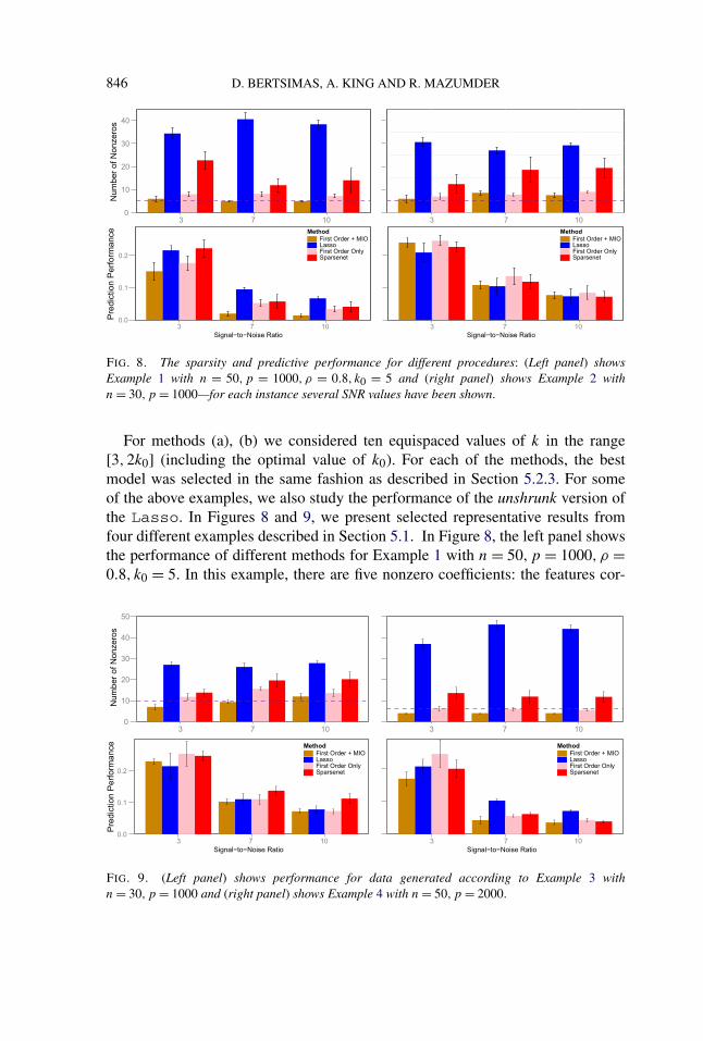
846 D. BERTSIMAS, A. KING AND R. MAZUMDER
FIG. 8. The sparsity and predictive performance for different procedures: (Left panel) showsExample 1 with n = 50,p = 1000, ρ = 0.8, k0 = 5 and (right panel) shows Example 2 withn = 30,p = 1000—for each instance several SNR values have been shown.
For methods (a), (b) we considered ten equispaced values of k in the range[3,2k0] (including the optimal value of k0). For each of the methods, the bestmodel was selected in the same fashion as described in Section 5.2.3. For someof the above examples, we also study the performance of the unshrunk version ofthe Lasso. In Figures 8 and 9, we present selected representative results fromfour different examples described in Section 5.1. In Figure 8, the left panel showsthe performance of different methods for Example 1 with n = 50,p = 1000, ρ =0.8, k0 = 5. In this example, there are five nonzero coefficients: the features cor-
FIG. 9. (Left panel) shows performance for data generated according to Example 3 withn = 30,p = 1000 and (right panel) shows Example 4 with n = 50,p = 2000.

BEST SUBSET SELECTION VIA A MODERN OPTIMIZATION LENS 847
responding to the nonzero coefficients are weakly correlated and a feature havinga nonzero coefficient is highly correlated with a feature having a zero coefficient(in the generating model). In this situation, the Lasso selects a very dense modelsince it fails to distinguish between a zero and a nonzero coefficient when the vari-ables are correlated—it brings both the coefficients in the model (with shrinkage).MIO (with warm-start) performs the best—both in terms of predictive accuracyand in selecting a sparse set of coefficients. MIO obtains the sparsest model amongthe four methods and seems to find better solutions in terms of statistical propertiesthan the models obtained by the first-order methods alone. Interestingly, the “op-timal model” selected by the first-order methods is more dense than that selectedby the MIO. The number of nonzero coefficients selected by MIO remains fairlystable across different SNR values, unlike the other three methods. For this ex-ample, we also experimented with the different versions of unshrunk Lasso [seeresults in Bertsimas, King and Mazumder (2015), Section 10.2 for details]. In sum-mary: the best unshrunk Lasso models had performance marginally better thanLasso but quite inferior to MIO. Figure 8 (right panel) shows Example 2, withn = 30,p = 1000, k0 = 5 and all nonzero coefficients equal one. Here, all methodsperform similarly in terms of predictive accuracy. In fact, for the smallest value ofSNR, the Lasso achieves the best predictive model. In all of the cases, however,the MIO achieves the sparsest model with favorable predictive accuracy. In Fig-ure 9, for both the examples, the model matrix is an i.i.d. Gaussian ensemble. Theunderlying regression coefficient β0 however, is structurally different than Exam-ple 2 (as in Figure 8, right-panel). The alternating signs of β0 is responsible for dif-ferent statistical behaviors of the four methods across Figures 8 (right-panel) andFigure 9 (both panels). The MIO (with warm-starts) seems to be the best amongall the methods. For Example 3 (Figure 9, left panel), the predictive performancesof Lasso and MIO are comparable—the MIO, however, delivers much sparsermodels than the Lasso.
The key conclusions are as follows:
1. The MIO best subset algorithm has a significant edge in detecting the cor-rect sparsity structure for all examples compared to Lasso, Sparsenet and thestand-alone discrete first-order method.
2. For data generated as per Example 1 with large values of ρ, the MIO bestsubset algorithm gives better predictive performance compared to its competitors.
3. For data generated as per Examples 2 and 3, MIO delivers similar predictivemodels like the Lasso, but produces much sparser models. In fact, Lasso seemsto perform marginally better than MIO, as a predictive model for small values ofSNR.
4. For Example 4, MIO performs the best both in terms of predictive accuracyand delivering sparse models.

848 D. BERTSIMAS, A. KING AND R. MAZUMDER
6. Computations for subset selection with least absolute deviation loss.Herein, we study the properties of the best subset selection problem with LADobjective (3.13) via a few representative examples. The LAD loss is appropriatewhen the error follows a heavy-tailed distribution. The datasets used for the exper-iments parallel those described in Section 5.1, the difference being in the distribu-tion of ε. We took εi i.i.d. from a double exponential distribution with variance σ 2.The value of σ 2 was adjusted to get different values of SNR.
Datasets analysed. We consider a set-up similar to Example 1 (Section 5.1)with k0 = 5 and ρ = 0.9. Different choices of (n,p) were taken to cover boththe overdetermined (n = 500,p = 100) and high-dimensional cases (n = 50,p =1000 and n = 500,p = 1000).
Other methods used for comparison were (a) discrete first-order method (Sec-tion 3.3) (b) MIO warm-started with the first-order solutions and (c) the LAD losswith �1 regularization:
min‖y − Xβ‖1 + λ‖β‖1,
which we denote by LAD-Lasso. The training, validation and testing were donein the same fashion as in the least squares case. For each method, we report thenumber of nonzeros in the optimal model and associated prediction accuracy (5.2).
Figure 10 (left panel) compares the MIO approach with others for the overdeter-mined case (n > p). Figure 10 (middle and right panels) do the same for the high-dimensional case (p � n). The conclusions parallel those for the least squares
FIG. 10. Figure showing the number of nonzero values and predictive performance for differentvalues of n and p for problem (3.13). The data is generated as per Example 1 with ρ = 0.9, k0 = 5,for different problem sizes—(left panel) n = 500,p = 100; (middle panel) n = 50,p = 1000 and(right panel) n = 500,p = 1000. The acronym “Lasso” refers to LAD-Lasso. MIO is seen todeliver sparser models with better predictive accuracy when compared to the LAD-Lasso.

BEST SUBSET SELECTION VIA A MODERN OPTIMIZATION LENS 849
case. Since, in the example considered, the features corresponding to the nonzerocoefficients are weakly correlated and a feature having a nonzero coefficient ishighly correlated with a feature having a zero coefficient—the LAD-Lasso se-lects an overly dense model and misses out in terms of prediction error. Both theMIO (with warm-starts) and the discrete first-order methods behave similarly—much better than �1 regularization schemes. As expected, we observed that subsetselection with least squares loss leads to inferior models for these examples, dueto a heavy-tailed distribution of the errors.
Our findings here are similar to that in the least squares case. The MIO approachprovides an edge both in terms of sparsity and predictive accuracy compared toLasso both for the overdetermined and the high-dimensional case.
7. Conclusions. In this paper, we have revisited the classical best subset se-lection problem of choosing k out of p features in linear regression given n obser-vations using a modern optimization lens—MIO and a discrete extension of first-order methods from continuous optimization. Exploiting the astonishing progressof MIO solvers in the last twenty-five years, we have shown that this approachsolves problems with n in the 1000s and p in the 100s in minutes to provable opti-mality, and finds near optimal solutions for n in the 100s and p in the 1000s in min-utes. Importantly, the solutions provided by the MIO approach often significantlyoutperform other state of the art methods like Lasso in achieving sparse modelswith good predictive power. Unlike all other methods, the MIO approach alwaysprovides a guarantee on its suboptimality even if the algorithm is terminated early.Moreover, it can accommodate side constraints on the coefficients of the linearregression and also extends to finding best subset solutions for the least absolutedeviation loss function. While continuous optimization methods have played andcontinue to play an important role in statistics over the years, discrete optimiza-tion methods have not. The evidence in this paper as well as in Bertsimas andMazumder (2014) suggests that MIO methods are tractable and lead to desirableproperties (improved accuracy and sparsity among others) at the expense of higher,but still reasonable, computational times.
Acknowledgments. We would like to thank the Associate Editor and twoanonymous reviewers for their comments that helped us improve the paper.
SUPPLEMENTARY MATERIAL
Supplement to “Best subset selection via a modern optimization lens” (DOI:10.1214/15-AOS1388SUPP; .pdf). Supporting technical material and additionalexperimental results including some figures and tables are presented in the supple-mentary material section.

850 D. BERTSIMAS, A. KING AND R. MAZUMDER
REFERENCES
BANDEIRA, A. S., DOBRIBAN, E., MIXON, D. G. and SAWIN, W. F. (2013). Certifying the re-stricted isometry property is hard. IEEE Trans. Inform. Theory 59 3448–3450. MR3061257
BERTSIMAS, D., KING, A. and MAZUMDER, R. (2015). Supplement to “Best subset selection viaa modern optimization lens.” DOI:10.1214/15-AOS1388SUPP.
BERTSIMAS, D. and MAZUMDER, R. (2014). Least quantile regression via modern optimization.Ann. Statist. 42 2494–2525. MR3277669
BERTSIMAS, D. and SHIODA, R. (2009). Algorithm for cardinality-constrained quadratic opti-mizaiton. Comput. Optim. Appl. 43 1–22. MR2501042
BERTSIMAS, D. and WEISMANTEL, R. (2005). Optimization Over Integers. Dynamic Ideas, Bel-mont.
BICKEL, P. J., RITOV, Y. and TSYBAKOV, A. B. (2009). Simultaneous analysis of lasso and Dantzigselector. Ann. Statist. 37 1705–1732. MR2533469
BIENSTOCK, D. (1996). Computational study of a family of mixed-integer quadratic programmingproblems. Math. Programming 74 121–140. MR1406746
BIXBY, R. E. (2012). A brief history of linear and mixed-integer programming computation. Doc.Math. Extra Volume: Optimization Stories 107–121. MR2991475
BLUMENSATH, T. and DAVIES, M. E. (2008). Iterative thresholding for sparse approximations.J. Fourier Anal. Appl. 14 629–654. MR2461601
BLUMENSATH, T. and DAVIES, M. E. (2009). Iterative hard thresholding for compressed sensing.Appl. Comput. Harmon. Anal. 27 265–274. MR2559726
BÜHLMANN, P. and VAN DE GEER, S. (2011). Statistics for High-Dimensional Data: Methods,Theory and Applications. Springer Series in Statistics. Springer, Heidelberg. MR2807761
BUNEA, F., TSYBAKOV, A. B. and WEGKAMP, M. H. (2007). Aggregation for Gaussian regression.Ann. Statist. 35 1674–1697. MR2351101
CANDÈS, E. J. (2008). The restricted isometry property and its implications for compressed sensing.C. R. Math. Acad. Sci. Paris 346 589–592. MR2412803
CANDÈS, E. J. and PLAN, Y. (2009). Near-ideal model selection by �1 minimization. Ann. Statist.37 2145–2177. MR2543688
CANDES, E. J. and TAO, T. (2006). Near-optimal signal recovery from random projections: Univer-sal encoding strategies? IEEE Trans. Inform. Theory 52 5406–5425. MR2300700
CANDÈS, E. J., WAKIN, M. B. and BOYD, S. P. (2008). Enhancing sparsity by reweighted l1minimization. J. Fourier Anal. Appl. 14 877–905. MR2461611
CHEN, S. S., DONOHO, D. L. and SAUNDERS, M. A. (1998). Atomic decomposition by basispursuit. SIAM J. Sci. Comput. 20 33–61. MR1639094
DETTLING, M. (2004). Bagboosting for tumor classification with gene expression data. Bioinfor-matics 20 3583–3593.
DONOHO, D. L. (2006). For most large underdetermined systems of linear equations the minimall1-norm solution is also the sparsest solution. Comm. Pure Appl. Math. 59 797–829. MR2217606
DONOHO, D. L. and ELAD, M. (2003). Optimally sparse representation in general (nonorthogo-nal) dictionaries via l1 minimization. Proc. Natl. Acad. Sci. USA 100 2197–2202 (electronic).MR1963681
DONOHO, D. L. and HUO, X. (2001). Uncertainty principles and ideal atomic decomposition. IEEETrans. Inform. Theory 47 2845–2862. MR1872845
DONOHO, D. L. and JOHNSTONE, I. M. (1994). Ideal spatial adaptation by wavelet shrinkage.Biometrika 81 425–455. MR1311089
EFRON, B., HASTIE, T., JOHNSTONE, I. and TIBSHIRANI, R. (2004). Least angle regression. Ann.Statist. 32 407–499. MR2060166
FAN, J. and LI, R. (2001). Variable selection via nonconcave penalized likelihood and its oracleproperties. J. Amer. Statist. Assoc. 96 1348–1360. MR1946581

BEST SUBSET SELECTION VIA A MODERN OPTIMIZATION LENS 851
FAN, J. and LV, J. (2011). Nonconcave penalized likelihood with NP-dimensionality. IEEE Trans.Inform. Theory 57 5467–5484. MR2849368
FAN, Y. and LV, J. (2013). Asymptotic equivalence of regularization methods in thresholded param-eter space. J. Amer. Statist. Assoc. 108 1044–1061. MR3174683
FRANK, I. and FRIEDMAN, J. (1993). A statistical view of some chemometrics regression tools(with discussion). Technometrics 35 109–148.
FRIEDMAN, J. (2008). Fast sparse regression and classification. Technical report, Dept. Statistics,Stanford Univ., Stanford, CA.
FRIEDMAN, J., HASTIE, T., HÖFLING, H. and TIBSHIRANI, R. (2007). Pathwise coordinate opti-mization. Ann. Appl. Stat. 1 302–332. MR2415737
FURNIVAL, G. and WILSON, R. (1974). Regression by leaps and bounds. Technometrics 16 499–511.
GREENSHTEIN, E. (2006). Best subset selection, persistence in high-dimensional statistical learningand optimization under l1 constraint. Ann. Statist. 34 2367–2386. MR2291503
GREENSHTEIN, E. and RITOV, Y. (2004). Persistence in high-dimensional linear predictor selectionand the virtue of overparametrization. Bernoulli 10 971–988. MR2108039
GUROBI, I. (2013). Optimization. Gurobi optimizer reference manual. Available at http://www.gurobi.com.
HASTIE, T., TIBSHIRANI, R. and FRIEDMAN, J. (2009). The Elements of Statistical Learning: DataMining, Inference, and Prediction, 2nd ed. Springer Series in Statistics. Springer, New York.MR2722294
KNIGHT, K. and FU, W. (2000). Asymptotics for lasso-type estimators. Ann. Statist. 28 1356–1378.MR1805787
LOH, P.-L. and WAINWRIGHT, M. (2013). Regularized M-estimators with nonconvexity: Statisticaland algorithmic theory for local optima. In Advances in Neural Information Processing Systems476–484. Curran Associates, Red Hook, NY.
LV, J. and FAN, Y. (2009). A unified approach to model selection and sparse recovery using regular-ized least squares. Ann. Statist. 37 3498–3528. MR2549567
MAZUMDER, R., FRIEDMAN, J. H. and HASTIE, T. (2011). SparseNet: Coordinate descent withnonconvex penalties. J. Amer. Statist. Assoc. 106 1125–1138. MR2894769
MEINSHAUSEN, N. and BÜHLMANN, P. (2006). High-dimensional graphs and variable selectionwith the lasso. Ann. Statist. 34 1436–1462. MR2278363
MILLER, A. (2002). Subset Selection in Regression, 2nd ed. Monographs on Statistics and AppliedProbability 95. Chapman & Hall/CRC, Boca Raton, FL. MR2001193
NATARAJAN, B. K. (1995). Sparse approximate solutions to linear systems. SIAM J. Comput. 24227–234. MR1320206
NEMHAUSER, G. (2013). Integer programming: The global impact. 2013–12–2013–04, Rome, Italy.Presented at EURO, INFORMS, Accessed. Available at https://smartech.gatech.edu/handle/1853/49829.
NESTEROV, Y. (2004). Introductory Lectures on Convex Optimization: A Basic Course. AppliedOptimization 87. Kluwer Academic, Boston, MA. MR2142598
NESTEROV, YU. (2005). Smooth minimization of non-smooth functions. Math. Program. 103 127–152. MR2166537
NESTEROV, YU. (2013). Gradient methods for minimizing composite functions. Math. Program.140 125–161. MR3071865
OPTIMIZATION INC. (2015). Gurobi 6.0 performance benchmarks. Available at http://www.gurobi.com/pdfs/benchmarks.pdf. Accessed 5 September 2015.
RASKUTTI, G., WAINWRIGHT, M. J. and YU, B. (2011). Minimax rates of estimation forhigh-dimensional linear regression over �q -balls. IEEE Trans. Inform. Theory 57 6976–6994.MR2882274

852 D. BERTSIMAS, A. KING AND R. MAZUMDER
SHEN, X., PAN, W., ZHU, Y. and ZHOU, H. (2013). On constrained and regularized high-dimensional regression. Ann. Inst. Statist. Math. 65 807–832. MR3105798
TIBSHIRANI, R. (1996). Regression shrinkage and selection via the lasso. J. Roy. Statist. Soc. Ser. B58 267–288. MR1379242
TIBSHIRANI, R. (2011). Regression shrinkage and selection via the lasso: A retrospective. J. R. Stat.Soc. Ser. B Stat. Methodol. 73 273–282. MR2815776
TOP500 SUPERCOMPUTER SITES (2015). Directory page for Top500 lists. In Result for each listsince June 1993. Accessed: 09-15-2015. Available at http://www.top500.org/statistics/sublist/.
TROPP, J. A. (2006). Just relax: Convex programming methods for identifying sparse signals innoise. IEEE Trans. Inform. Theory 52 1030–1051. MR2238069
VAN DE GEER, S., BÜHLMANN, P. and ZHOU, S. (2011). The adaptive and the thresholded Lassofor potentially misspecified models (and a lower bound for the Lasso). Electron. J. Stat. 5 688–749. MR2820636
WAINWRIGHT, M. J. (2009). Sharp thresholds for high-dimensional and noisy sparsity recoveryusing �1-constrained quadratic programming (Lasso). IEEE Trans. Inform. Theory 55 2183–2202.MR2729873
ZHANG, C.-H. (2010a). Nearly unbiased variable selection under minimax concave penalty. Ann.Statist. 38 894–942. MR2604701
ZHANG, T. (2010b). Analysis of multi-stage convex relaxation for sparse regularization. J. Mach.Learn. Res. 11 1081–1107. MR2629825
ZHANG, C.-H. and HUANG, J. (2008). The sparsity and bias of the LASSO selection in high-dimensional linear regression. Ann. Statist. 36 1567–1594. MR2435448
ZHANG, Y., WAINWRIGHT, M. and JORDAN, M. I. (2014). Lower bounds on the performance ofpolynomial-time algorithms for sparse linear regression. Preprint. Available at arXiv:1402.1918.
ZHANG, C.-H. and ZHANG, T. (2012). A general theory of concave regularization for high-dimensional sparse estimation problems. Statist. Sci. 27 576–593. MR3025135
ZHAO, P. and YU, B. (2006). On model selection consistency of Lasso. J. Mach. Learn. Res. 72541–2563. MR2274449
ZHENG, Z., FAN, Y. and LV, J. (2014). High dimensional thresholded regression and shrinkageeffect. J. R. Stat. Soc. Ser. B. Stat. Methodol. 76 627–649. MR3210731
ZOU, H. (2006). The adaptive lasso and its oracle properties. J. Amer. Statist. Assoc. 101 1418–1429.MR2279469
ZOU, H. and LI, R. (2008). One-step sparse estimates in nonconcave penalized likelihood models.Ann. Statist. 36 1509–1533. MR2435443
D. BERTSIMAS
R. MAZUMDER
MIT SLOAN SCHOOL OF MANAGEMENT
AND OPERATIONS RESEARCH CENTER
MASSACHUSETTS INSTITUTE OF TECHNOLOGY
CAMBRIDGE, MASSACHUSETTS
USAE-MAIL: [email protected]
A. KING
OPERATIONS RESEARCH CENTER
MASSACHUSETTS INSTITUTE OF TECHNOLOGY
CAMBRIDGE, MASSACHUSETTS
USAE-MAIL: [email protected]