better luck next time · better luck next time: learning through retaking verónica frisancho, kala...
TRANSCRIPT

NBER WORKING PAPER SERIES
BETTER LUCK NEXT TIME:LEARNING THROUGH RETAKING
Verónica FrisanchoKala Krishna
Sergey LychaginCemile Yavas
Working Paper 19663http://www.nber.org/papers/w19663
NATIONAL BUREAU OF ECONOMIC RESEARCH1050 Massachusetts Avenue
Cambridge, MA 02138November 2013
We are grateful to the Center for University Selection and Placement (O SYM) for providing the data.We would also like to thank Dilara Bakan Kalayc�oglu for answering all our questions about the dataand Quang Vuong and Susumu Imai for extremely useful conversations. We are also indebted to participantsof the Pacific Conference for Development Economics 2011, the 10th Journees Louis-André Gérard-VaretConference in Public Economics, the LACEA 2012 Annual Meeting, the 2012 Seminar Series at theCopenhagen Business School, the 8th Annual Conference on Economic Growth and Developmentat ISI Delhi, and the 2012 Asian Meeting of the Econometric Society for suggestions and comments.Kala Krishna would like to thank the Human Capital Foundation (www.hcfoundation.ru), and especiallyAndrey P. Vavilov, for support of the Department of Economics at Penn State University. The viewsexpressed herein are those of the authors and do not necessarily reflect the views of the National Bureauof Economic Research.
At least one co-author has disclosed a financial relationship of potential relevance for this research.Further information is available online at http://www.nber.org/papers/w19663.ack
NBER working papers are circulated for discussion and comment purposes. They have not been peer-reviewed or been subject to the review by the NBER Board of Directors that accompanies officialNBER publications.
© 2013 by Verónica Frisancho, Kala Krishna, Sergey Lychagin, and Cemile Yavas. All rights reserved.Short sections of text, not to exceed two paragraphs, may be quoted without explicit permission providedthat full credit, including © notice, is given to the source.

Better Luck Next Time: Learning Through RetakingVerónica Frisancho, Kala Krishna, Sergey Lychagin, and Cemile YavasNBER Working Paper No. 19663November 2013JEL No. C13,C38,I23,I24
ABSTRACT
In this paper we provide some evidence that repeat taking of competitive exams may reduce theimpact of background disadvantages on educational outcomes. Using administrative data on the university entrance exam in Turkey we estimate cumulative learning between the first and the nthattempt while controlling for selection into retaking in terms of observed and unobserved characteristics.We find large learning gains measured in terms of improvements in the exam scores, especially amongless advantaged students.
Verónica FrisanchoResearch DepartmentInter-American Development Bank (IADB)1300 New York Ave. NWWashington, DC [email protected]
Kala KrishnaDepartment of Economics523 Kern Graduate BuildingThe Pennsylvania State UniversityUniversity Park, PA 16802and [email protected]
Sergey LychaginDepartment of EconomicsCentral European UniversityNador u. 9Budapest [email protected]
Cemile [email protected]
1 Introduction
A central question in education policy is how to reduce the dependence of educational outcomes
on background. In this paper we provide evidence that repeat taking of entrance exams might
have some promise in this regard. Using administrative data on the university entrance exam
(OSS) in Turkey we estimate cumulative learning in repeated attempts, while controlling for
selection into retaking in terms of observed and unobserved characteristics. Our contribution
is twofold. First, we provide a simple way to estimate learning gains among retakers despite
only having cross-sectional data. Second, we find large learning gains, measured in terms of
improvements in the entrance exam scores, especially among less advantaged students.
We use administrative data on a random sample of about 115,000 OSS applicants (of which
only about a third are first time takers) from three high school tracks (Science, Social Studies,
Turkish/Math). Estimating learning gains from retaking is particularly challenging for us as
we cannot follow students as would be possible with panel data. However, we overcome this
limitation using information on repeat takers along with a rich set of performance measures.
Our approach controls for selection into retaking and teases out average cumulative learning
between the first and nth attempts.
Our model’s key assumptions are i) students know their own ability though it is unobserved
by the econometrician, ii) learning is a draw from a distribution that is allowed to vary with
observables and/or unobservables, and iii) performance in high school and on the entrance exam
is partly determinate, coming from observables and unobserved ability, and partly random. We
take a factor approach where the factors are the random performance shocks and the unobserved
ability. In our model ability will drive the correlation between high school grade point average
(GPA) and raw verbal and quantitative exam scores once the effect of observables is netted out.
We find important cumulative learning gains among repeat takers once selection into retaking
is controlled for. For example, we find that learning gains in the second attempt fluctuate around
5% of the predicted initial score, irrespective of the track. In the Social Studies and Turkish-
Math tracks, we identify larger and increasing cumulative gains as the number of attempts
1

increases. Gains in these two tracks on higher order attempts range from 8% to 14% of the
predicted initial score.
Most important, we identify larger gains among repeat takers from less advantaged back-
grounds: in all tracks, students who come from public schools and households in the lowest in-
come category experience larger learning gains than more privileged students from elite schools
or higher income households. These results suggest that disadvantaged students can meet high
admission standards though it may take them multiple attempts to do so. Although in this
paper we do not (and cannot) measure the net welfare impact of allowing retaking, our results
draw attention to the benefits that systems like the Turkish one, similar to that in much of
continental Europe, Asia, and some Latin American countries, may generate for repeat takers.
While we focus on the Turkish experience, the issues we study are far more general. Most
countries rely on different admissions systems to place students. The extent to which they rely
exclusively on an exam or on a more diverse spectrum of student characteristics varies consider-
ably. In the US, for example, the SAT or ACT is widely used. However, performance on these
exams is only a small part of what colleges use in admissions decisions. Extracurricular activi-
ties, alumni ties, interviews, the perceived likelihood of the student coming, and donations may
matter even more than the student’s performance. As long as these factors favor more privi-
leged students, such an allocation system will tend to perpetuate socioeconomic inequalities. By
eliminating the direct influence of socioeconomic status on school placement, the Turkish system
offers a way to level the playing field for less advantaged students. Moreover, though students’
backgrounds will still have an effect on performance indirectly, allowing multiple attempts may
enable less prepared but able students to catch up and reduce the role of background inequalities
on college admissions outcomes.
The paper proceeds as follows. Section 2 relates our work to the literature. Section 3
describes the institutional context and the data. The model and the econometric methodology
are presented in Section 4 while Section 5 presents the results. Finally, Section 6 concludes and
lays out some avenues for future research.
2

2 Related Literature
By documenting that the learning gains of repeat taking are higher for more disadvantaged
students, our paper relates to two strands of literature on educational catch-up.
The first of these strands looks at the issue of catch-up by immigrants. Portes and Rumbaut
(2001) found that immigrant children who arrive before age 13 and second generation children
in Miami and San Diego tend to perform better than their native-born schoolmates in terms of
grades, rates of school retention, and behavioral aspects (e.g., doing homework). However, those
who arrive after age 13 tend to be outperformed by native-born students. Using the 1995-2002
Current Population Surveys (CPS), Card (2005) finds some evidence in favor of educational
catch-up among second generation migrants. While immigrants have about 1.2–1.4 fewer years
of education than natives, second generation immigrants have 0.3–0.4 more years of schooling
than people whose parents were born in the US.
The second strand, which focuses on disadvantaged groups favored by affirmative action
(AA), presents a less rosy picture. In general, rather than catching-up, the beneficiaries of
AA preferences seem to fall behind. Sander (2004) finds that the average performance gap
between blacks and whites at selective law schools is large and, more importantly, tends to get
larger as both groups progress through school. Arcidiacono et al. (2012) shows that the GPA
gap between white and black students at Duke University falls by half between the first and
the last year of college, but this comes primarily from smaller variance in grading during later
years and a higher proportion of black students switching into easier majors. If weaker students
choose easier courses and this self-selection is not taken into account, one might incorrectly
interpret a reduction in the academic gap between strong and weak students as catch-up. Loury
and Garman (1993, 1995) make a related point. In settings where course selection issues are
minimized, students given preferences seem to fall behind. Frisancho and Krishna (2012) look at
the Indian higher education setting which has transparent admission criteria and a rigid course
structure as well as significant affirmative action. They find that backward groups fall behind,
and more so in more selective majors where the initial gap is greater.
3

In our setting, the exam covers the same set of subjects and has the same level of difficulty
across cohorts. This generates two advantages: i) we do not have to deal with self-selection
into majors and courses and ii) it is easier to catch up in our setting than in the AA case. The
beneficiaries of AA admission policies start college lacking prerequisite knowledge and cannot
benefit from college-level courses to the same extent as their more prepared peers. Consequently,
even by running as fast as they can, these students can hope, at best, to stay in the same place
they started.
Although relatively scarce, there have been previous attempts to measure catch-up in an
environment similar to ours, that is, in the period between high school graduation and college
enrollment. Nathan and Camara (1998) shows that 55% (35%) of the juniors taking the SAT
in the US improved (worsened) their scores as seniors. Vigdor and Clotfelter (2003) use data
on undergraduate applicants to three selective US research universities to look at the evolution
of SAT scores over multiple attempts. They implement a two-stage Heckman sample-selection
procedure and estimate that between 70% and 90% of the observed score increase remains when
selection is accounted for.
Although the contribution of the work on SATs is important, there are two important dis-
advantages compared to the OSS. First, as the SATs are one of many things that matter for
university admissions, students take them more lightly, generating noisier measures of perfor-
mance. Second, the level of difficulty of the SAT is far below that of the OSS, with the SAT
being more of an IQ test than a skills test. This compromises its ability to distinguish between
takers, especially at the high end. Thus, we argue that our data provides important advantages
to looking for evidence on catch-up and measuring learning among repeat takers.
Our methodology imposes a factor structure on performance outcomes in high school and on
the admission exam. Net of the effects of observables, GPA and exam scores are determined by
two factors: students’ ability and randomness. Following Carneiro et al. (2003), many papers
have relied on this structure to model educational outcomes.1
1See for example, Cooley et al. (2011).
4

3 Turkish Context
3.1 Institutional Background
In Turkey, entrance to higher education institutions is regulated by the OSS (Student Selection
Exam), a national examination administered by the Student Selection and Placement Center
(OSYM) on an annual basis. All high school seniors and graduates are eligible to take it and
there is no limit on the number of retakes.2 Even though centralized admission systems are
common in other places in Europe as well as Asia and Latin America, the Turkish setting is
particularly interesting due to the high share of repeat takers in the pool of applicants. For
instance, in 2002 roughly one-third of the exam takers were high school seniors, the remainder
being repeat takers.3 Although the high ratio of retakers coupled with a low placement rate
seems wasteful, there may be some hidden benefits of the current setup.
The college placement exam is composed of multiple choice questions with negative marking
for incorrect answers. Students’ performance is evaluated in four subjects: Mathematics, Turk-
ish, Science, and Social Studies. The raw scores in these four subjects are then used to calculate
raw verbal scores, defined as the sum of the scores in Turkish and Social Studies, and raw quan-
titative scores, defined as the sum of Science and Math. All the raw scores are standardized and
used to construct three weighted scores.4 Students who obtain more than 105 in any weighted
score are eligible to submit preferences for two year schools or distance education programs. To
be able to submit preferences for four year programs, a minimum score of 120 is required.
Students choose a track while in high school; for the most part, the choice is between Sciences,
Social Studies, and Turkish-Math. The college placement process is designed to encourage
students to apply to programs that build on their high school education.5 Depending on the
college program chosen by the student, only one of the three weighted scores will be relevant.
This setup enables us to focus on a single weighted score for each track, which we call the relevant
2See Turk Egitim Dernegi (TED or Turkish Educational Association) for more details on this exam.3The most recent ratio of high school seniors to total candidates, although higher, is still quite low: in 2013,
there were about 800,000 high school seniors among 1.9 million applications.4For details, see Appendix A.5For example, the high school GPA of someone from the Science track is given less weight if he applies to a
program compatible with another track.
5

exam score in the following sections. OSYM also calculates placement scores for each subject,
which are a combination of the weighted scores and a standardized measure of the student’s
high school GPA.6
Once the applicant learns his scores, he submits a list of his program preferences, having
complete information on the previous year’s cut-off scores for each program (i.e., the score of
the last student admitted). Placement is merit based: a student is placed in his most preferred
program, conditional on the availability of seats after all the applicants with higher scores are
placed. Students fail to be placed if they do not pass the exam or if other students with better
scores fill up all the available seats in the programs on their preference list. These students
will have the option of retaking the exam with no penalties. Students who are placed are also
allowed to retake, but their placement score is penalized if they retake the following year.
3.2 Data
Our data covers a random sample of about 120,000 students who took the OSS in 2002. After
cleaning the data and dealing with some minor inconsistencies, we lose 3.9% of the observations
so that our final cross section covers 114,800 applicants from the Science (38,771), Turkish-Math
(38,571), and Social Studies tracks (37,458).
OSYM data comes from four sources: students’ application forms, a survey applied in 2002,
high school records, and administrative records. For each student, our database contains infor-
mation on high school characteristics (track and type of school), high school GPA, standing at
the time of the exam (high school senior, repeat taker, graduated from another program, among
other options), individual and background characteristics (gender, household income, parents’
education and occupation, family size, time and money spent on private tutoring, and number
of previous attempts), and performance outcomes (raw scores, weighted scores, and placement
outcomes). Since we want to measure high school performance across schools, we construct
quality normalized GPAs to control for quality heterogeneity and grade inflation across high
6This standardization is implemented by the OSYM to make GPAs comparable. A detailed description of thisprocess is provided in Appendix A.
6

schools (see Appendix B for details).7
3.3 Preliminary Evidence
The measurement of learning gains among repeat takers would be a straightforward exercise with
longitudinal data. However, the OSS data only provides us with a cross-section of applicants,
both first time takers as well as repeat takers.
Although the scores of repeat takers will contain information on learning relative to their
first attempt, it is hard to isolate these gains without a counterfactual. Notice that the exam
scores of repeat takers reflect two effects: learning and selection into retaking. Learning shifts
the distribution of scores to the right over attempts while selection, which is an endogenous
process, can shift it to the right or to the left depending on who retakes.
Figure 1: Distribution of Exam Scores by Track
0.0
1.0
2.0
3.0
4.0
5.0
6D
ensi
ty
80 100 120 140 160 180 200Exam Score
Science
0.0
1.0
2.0
3.0
4.0
5.0
6D
ensi
ty
70 90 110 130 150 170Exam Score
Social Studies
0.0
1.0
2.0
3.0
4.0
5.0
6D
ensi
ty
80 100 120 140 160 180Exam Score
Turkish−Math
1st 2nd 3rd 4th 5th or more
Figure 1 plots the empirical distributions of exam scores by number of attempts and track.
In general, there is some evidence of compression in the distributions as the number of attempts
increases. Yet, two distinct patterns emerge. In the Science track the distribution of scores
shifts to the left, consistent with worse students selecting into retaking and limited learning. In
7It is worth noting that very few papers have explored the Turkish data set. Tansel and Bircan (2005) studiesthe determinants of attendance at private tutoring centers and its effects on performance. Saygin (2011) looksat the gender gap in college. Moreover, Caner and Okten (2010) looks at career choice using data on preferenceswhile Caner and Okten (2013) examines how the benefits of publicly subsidized higher education are distributedamong students with different socioeconomic backgrounds.
7

turn, the score distribution moves to the right in Turkish-Math and Social Studies. This could
suggest sizeable learning gains but selection could be operating in either direction.
A further look into the data identifies a pattern common to all tracks. Figure 2 presents exam
score distributions by number of attempts and high school GPA quartiles. In all tracks, first
time takers do worse than repeat takers in the lowest GPA quartiles but this pattern reverses as
GPA increases. This suggests that weaker students learn more.8 If better performing students
are disproportionately found in the Science track, Figure 1 could reflect a composition effect due
to differential learning and selection across tracks.
Table C.1 shows that this is the case. We find stronger students in the Science track, where
the average standardized high school GPA is 51.7 as compared to 49 and 47.7 in Turkish-Math
and Social Studies respectively. Science track students also seem to be better off than Social
Studies and Turkish-Math students in terms of other background characteristics: they have more
educated and wealthier parents. They also tend to come from better schools and have higher
access to prep schools and/or tutoring while in high school.
The next section develops a simple dynamic model of learning and repeat taking to help
us understand the biases that selection introduces. In light of this model, we then develop our
estimation strategy.
4 Model
In this section we lay out a simple model and our estimation strategy. We show that while
students select into retaking based on ability and performance shocks on the entrance exam,
GPA performance shocks do not affect retaking when students are very patient. Based on this,
we lay out a strategy to identify and measure learning effects relying only on cross-sectional
data.
8This pattern is also shown in Vigdor and Clotfelter (2003) among SAT repeat takers, suggesting that initiallybetter performing students have the lowest learning gains.
8

Figure 2: Distribution of Exam Scores by GPA quartiles and Track
0.0
1.0
2.0
3.0
4.0
5.0
6D
ensi
ty
80 100 120 140 160 180 200Exam Score
Quartile I
0.0
1.0
2.0
3.0
4.0
5.0
6D
ensi
ty
80 100 120 140 160 180 200Exam Score
Quartile II
0.0
1.0
2.0
3.0
4.0
5.0
6D
ensi
ty
80 100 120 140 160 180 200Exam Score
Quartile III
0.0
1.0
2.0
3.0
4.0
5.0
6D
ensi
ty
80 100 120 140 160 180 200Exam Score
Quartile IV
1st 2nd 3rd 4th 5th or more
(a) Science
0.0
1.0
2.0
3.0
4.0
5.0
6D
ensi
ty
70 90 110 130 150 170Exam Score
Quartile I0
.01
.02
.03
.04
.05
.06
Den
sity
70 90 110 130 150 170Exam Score
Quartile II
0.0
1.0
2.0
3.0
4.0
5.0
6D
ensi
ty
70 90 110 130 150 170Exam Score
Quartile III
0.0
1.0
2.0
3.0
4.0
5.0
6D
ensi
ty
70 90 110 130 150 170Exam Score
Quartile IV
1st 2nd 3rd 4th 5th or more
(b) Social Studies
0.0
1.0
2.0
3.0
4.0
5.0
6D
ensi
ty
80 100 120 140 160 180Exam Score
Quartile I
0.0
1.0
2.0
3.0
4.0
5.0
6D
ensi
ty
80 100 120 140 160 180Exam Score
Quartile II
0.0
1.0
2.0
3.0
4.0
5.0
6D
ensi
ty
80 100 120 140 160 180Exam Score
Quartile III
0.0
1.0
2.0
3.0
4.0
5.0
6D
ensi
ty
80 100 120 140 160 180Exam Score
Quartile IV
1st 2nd 3rd 4th 5th or more
(c) Turkish-Math
9

Let s∗ denote the cut-off exam score for a candidate to be placed in a program.9 Although
critical, the relevant exam score for student i in his nth attempt, denoted by sin, is not all that
determines placement (see Section 3.2). For students with exam scores above s∗, placement
scores are obtained as a weighted average of the exam score, sin, and high school GPA, gi. We
assume the system has a continuum of college qualities. Since students with higher scores have
more options open to them, they will obtain higher utility. Normalizing the weight on exam
scores to one, the instantaneous college utility is specified as follows:
u(sin, gi) =
{
−∞ if sin < s∗sin + ηgi if sin ≥ s∗
Students with a score below s∗ (the cutoff for being eligible) cannot be placed according to
the rules. We set their utility from being placed at −∞ to reflect the impossibility of placement
while those with a cutoff above s∗ choose between being placed, retaking, and quitting.
We assume that student i’s high school GPA is given by:
gi = Xiα0 + θi + εi0 (1)
where εi0 is a random shock. The term Xiα0 captures the effect of observables on the GPA while
θi is an individual-specific component that captures the ability of the student. Both the effect
of observables and ability are known to the student, but θi is unobserved by the researcher.10
As described in the data section, the exam score comes from the performance on the verbal
and quantitative sections of the exam, appropriately weighted. Let sinq and sinv denote the
student’s quantitative and verbal scores respectively, and ωq and ωv be fixed known weights:
sinq = Xiα1q + βqθi + Λinq + εinq (2)
sinv = Xiα1v + βvθi + Λinv + εinv (3)
9As explained in Section 3, OSYM imposes a cut-off score to qualify for placement in university programs.10The known ability assumption is reasonable in the Turkish context. Although the exam is taken in 12th grade,
students start preparing for this exam as early as 9th grade. By the time they take the exam for the first time,they have already taken many practice exams and have a good idea of their expected performance.
10

where Λinj is the cumulative learning in topic j up to attempt n.11 We assume that students
know their future learning shocks and let Λinj depend on Xi and/or θi. εinj is a random shock
drawn from a density function common to all n and i for a given j = v, q. These transitory
shocks are meant to capture chance occurrences that could affect exam performance (e.g., getting
a question you did not expect) and are therefore assumed to be iid.
The exam score is a weighted average of the verbal and quantitative scores, and hence
sin = ωqsinq + ωvsinv
= Xiα1 + βθi + Λin + εin
= sin + εin.
The distribution of εin is given by F (.) for all i and n. After the student learns his score, he
decides whether to retake, quit, or be placed. If he decides to retake, he pays a cost ψ that is
incurred immediately, though the results of retaking are apparent only a year later and so are
discounted by δ. Thus, the value of retaking is given by:
Vin(sin, gi,Λi) = −ψ + δEεi(n+1)(max
[
Vi(n+1)(si(n+1), gi,Λi), u(si(n+1), gi), VQ]
)
where VQ is the value of quitting and Λi is the vector of all the learning shocks in all retaking
attempts.
4.1 Selection Into Retaking
Students who retake are those for whom retaking is better than the maximum of quitting and
being placed. There is selection on εi0 for those choosing between retaking and being placed as
well as for those choosing between retaking and quitting. In this section, we use a simplified
version of the model discussed above to understand the nature of the selection driven by εi0.
When choosing between retaking and quitting, students with high εi0 will be more likely to
11In what follows, we talk about raw quantitative and verbal scores for Science and Social Studies students asdefined in Sub-Section 3.1. This is natural because the pair of subjects used to construct these raw scores getthe same weight in the relevant weighted scores for these tracks. However, in the Turkish-Math track, we labelas “quantitative” and “verbal” the sum of the Turkish and Math scores and the sum of the Science and SocialStudies scores, respectively, to reflect equal weights of these pairs of subjects in the relevant weighted score.
11

retake as a higher value of the GPA shock increases Vin without affecting VQ. In other words,
students with low εi0 will quit. This makes the expected value of εi0 among retakers positive,
generating a negative bias in our learning estimates. As δ rises, Vin increases and more students
retake, reducing, but possibly not eliminating, this negative bias.
On the other hand, when choosing between retaking and placement, students with high εi0
will be less likely to retake and more likely to cash in their good GPA shocks. However, as we
show below, as δ approaches unity, this effect fades away. At δ = 1, there is no selection on the
basis of εi0, and hence no positive bias.
Assume that there is no additional learning beyond the first retake, Λin = λi2 ≡ λi. This
assumption makes the problem stationary after the first period as the expected score for student
i is constant for each period n ≥ 2: sin ≡ si = Xiα1 + βθi + λi. Let εi be the shock that makes
student i just retake, i.e., Vi = u(si, gi, εi). Given (1) and the definition of the instantaneous
utility, εi is defined by
Vi = Xiα1 + βθi + λi + εi + η (Xiα0 + θi + εi0) (4)
Given the stationary nature of the problem, Vi is defined by
Vi = −ψ + δF (εi)Vi + δ
∫
ε=εi
(Xiα1 + βθi + λi + ε+ η(Xiα0 + θi + εi0)) f(ε)dε (5)
Substituting for Vi from (4) and rearranging gives
(Xiα1 + βθi + λi + εi + η (Xiα0 + θi + εi0)) (1− δF (εi))
= −ψ + δ [1− F (εi)] [Xiα1 + βθi + λi + η(Xiα0 + θi + εi0)] + δ
∫
ε=εi
εf(ε)dε
which yields
εi(1− δF (εi)) = −ψ + δ
∫
ε=εi
εf(ε)dε− (1− δ) (Xiα1 + βθi + λi + η (Xiα0 + θi + εi0)) (6)
At δ = 1 this reduces to
εi(1− F (εi)) = −ψ +
∫
ε=εi
εf(ε)dε.
12

Notice that for δ = 1, εi is independent of εi0, and hence E(ε0|n) = E(ε0) = 0. The intuition
is simple. When students are impatient, they want to cash in their high GPA so that students
with high εi0 are less likely to retake, i.e., E(ε0|n) < E(ε0) = 0. As δ goes to one, this effect
vanishes as is clear from looking at the derivative of (6) with respect to εi0 :
∂εi
∂εi0= −
(1− δ)
(1− δF (εi))η ≤ 0.
In the extreme, when students are perfectly patient, the utility associated with their GPA shock
is fixed over time and hence does not affect their decision to retake.
To summarize, there are two sources of selection on εi0 among repeat takers. First, those
with low εi0’s may choose to quit rather than retake which tends to make E(ε0|n) positive.
Second, those with high εi0’s may choose to be placed rather than retake, which tends to make
E(ε0|n) negative. The latter source of selection vanishes when students are patient enough while
the former need not.12
4.2 Taking the Model to the Data
Of interest for estimation are equations (1), (2), and (3). To estimate learning, we need to find
a way to obtain unbiased estimates of the α’s and β’s which will let us control for selection into
retaking. This is what we turn to now.
In the model, there are four factors, (θi, εi0, εinq, εinv), that affect the various performance
measures. The factor loadings, βq and βv in (2) and (3), respectively, allow θi to have a
differential effect across performance measures. The other three factors, εi0, εinq, and εinv,
capture randomness in performance. In order to identify the loadings on ability we rely on the
following standard assumption in the literature on Factor Models.
Assumption 4.1 The factors θi, εi0, εinq, and εinv are orthogonal to each other and to the
observables.
12As the astute reader would notice, the selection on the basis of θi operates through the same channels as theselection on the basis of εi0. However, these two sources of selection differ when students are below the cutoff sothat even if there is no selection on εi0, there could be selection on θi.
13

Figure 3 summarizes our estimation strategy, starting with first time takers on the left hand
side of the diagram. In Turkey, practically every high school senior takes the university entrance
exam. For this reason, the sub-sample of first time takers is free of selection. In this sub-sample,
we can estimate the system of performance equations given in the box for first time takers.
Figure 3: Estimation Strategy
1st
Time Takers
gi = Xiα0 + θi + εi0
si1q = Xiα1 + βqθi + εi1q
si1v = Xiα2 + βvθi + εi1v
nthTime Takers
gi = Xiα0 + θi + εi0
sinq = Xiα1 + βqθi + Λinq + εinq
sinv = Xiα2 + βvθi + Λinv + εinv
rg = gi −Xiα0 = θi + εi0
rsq = sinq −Xiα1 = βqθi + Λinq + εinq
rsv = sinv −Xiα2 = βvθi + Λinv + εinv
E(rsq − βqrg|Ni = n) = E(
Λinq − βqεi0|Ni = n)
≈ E (Λinq|Ni = n)
E(rsv − βvrg|Ni = n) = E(
Λinv − βvεi0|Ni = n)
≈ E (Λinv|Ni = n)
STEP 1:
STEP 2:
STEP 3:
STEP 4:
E(Λin|Ni = n) = ωqE (Λinq|Ni = n) + ωv
E (Λinv|Ni = n)
α0, α1, α2
βq, βv
As there is no learning among first time takers, the correlation between error terms across
the three performance equations is driven by students’ unobservables. This allows us to obtain
α0, α1, α2 using ordinary least squares to separately estimate each performance equation in the
14

sample of first time takers.13 Let rg, rsq , and rsv denote the residuals from the three performance
equations. These residuals, given in step 2 in Figure 3, contain both the effect of unobservables
and random shocks to performance.
It can easily be seen that:
E(r2g) = E(θ2 + ε20) = σ2θ + σ2ε0 (7)
E(r2sq ) = E(β2qθ
2 + ε21q) = β2qσ2θ + σ2ε1q (8)
E(r2sv ) = E(β2vθ
2 + ε21v) = β2vσ2θ + σ2ε1v (9)
E(rgrsq) = E[(θ + ε0)(βqθ + ε1q)] = βqσ2θ (10)
E(rgrsv) = E[(θ + ε0)(βvθ + ε1v)] = βvσ2θ (11)
E(rsqrsv) = E[(βqθ + ε1q)(βvθ + ε1v)] = βqβvσ2θ (12)
Solving this system of equations allows us to identify factors’ variances and loadings non-
parametrically.14 Table C.3 in Appendix C reports these estimates from which we only require
βq and βv to measure learning.
With α0, α1, α2, βq, and βv we can then move forward to steps 2, 3 and 4 in Figure 3. In
step 2 we use these estimates to back out θ + εi0 for each agent. This is a noisy estimate of
ability at the individual level. However, given the pattern of selection shown in Sub-Section 4.1,
when agents are patient enough E[θi + εi0|Ni = n] yields an upper bound of the effect of θi on
performance for Ni = n, which implies that the estimates we provide are a lower bound of the
learning effect.
In step 3, we use this noisy estimate weighted by βj and subtract it from rsj ∀j = {q, v}.
In other words, the difference between the score and the predicted score based on observables
and the noisy estimate of θ will give us our estimate of learning between the first and the nth
attempt. Notice that, since we allowed the learning shocks distribution to depend on Xi, we
13Full results are shown in Table C.2 in Appendix C.14(12) divided by (11) yields βq. The ratio of (10) to βq yields σ2
θ while the ratio of (11) to σ2θ yields βv. The
difference between (7) and σ2θ gives us σ2
0. Similarly, the differences between (8) and βq
2σ2θ and (9) and βv
2σ2θ
yield σ2ε1q
and σ2ε1v
, respectively.
15

can also identify heterogeneous learning effects by conditioning both on Ni and background
variables.
The approach described above will work well if E(εi0|Ni = n) is small. We carry out
simulations to confirm that the bias coming from selection on εi0 is very close to zero (see Sub-
Section 5.2). Before proceeding to our results, we would like to emphasize that we estimate
cumulative learning for all n but cannot estimate learning between attempts. This comes from
further selection occurring for students who keep retaking.15
5 Results
Table 1 presents the estimated average cumulative learning gains for repeat takers in terms
of their absolute improvement in points. We find that cumulative learning gains on the first
retry are quite similar across tracks and amount to about 5% of the average predicted score on
their first attempt. While in the Science track cumulative learning remains at roughly the same
level across attempts, Social Studies and Turkish-Math exhibit cumulative learning gains that
are increasing in the number of attempts. By the fifth attempt, students from Social Studies
and Turkish-Math tracks record learning gains of up to 14% and 10% of their initial predicted
score, respectively. Moreover, as Figure 4 shows, learning gains are critical for crossing the 120
point threshold in Social Studies and Turkish-Math tracks while they are not that crucial for
the average repeat taker in the Science track.
5.1 Learning, Selection, and Composition Revisited
As explained earlier, the change in the distribution of scores across attempts presented in Figure
1 is driven both by selection and learning within each track. Table 2 decomposes E(sin|Ni =
n)−E(si1|Ni = 1) into selection due to Xi, θi and learning, to get a better idea of their relative
importance by track.
In the Science track, the first row, labelled E(sin|Ni = n)−E(si1|Ni = 1), shows that repeat
15Students are forward-looking and know their future learning shocks, which means that students with higherΛins will retake more times. This implies that the difference between cumulative learning in attempts n and(n+ 1) will contain selection into retaking based on learning itself.
16

Table 1: E(Λin|Ni = n) by Track
Attempts Science Social Studies Turkish-Math
n = 2 6.724 6.032 5.867(0.233) (0.263) (0.159)
n = 3 6.624 10.160 8.980(0.341) (0.302) (0.219)
n = 4 7.052 12.601 10.073(0.414) (0.354) (0.358)
n ≥ 5 4.893 15.211 10.822(0.475) (0.423) (0.574)
Figure 4: Improvement in Gap from s∗ by Track
100
110
120
130
140
150
Poin
ts
2nd 3rd 4th 5thNumber of Attempts
E(si1|Ni) E(si1+Λin|Ni) s*
(a) Science
100
110
120
130
140
150
Poin
ts
2nd 3rd 4th 5thNumber of Attempts
E(si1|Ni) E(si1+Λin|Ni) s*
(b) Social Studies
100
110
120
130
140
150
Poin
ts
2nd 3rd 4th 5thNumber of Attempts
E(si1|Ni) E(si1+Λin|Ni) s*
(c) Turkish-Math
takers seem to be doing worse than first time takers on average, i.e., the density in Figure 1
moves backwards. The table shows that this is due to negative selection in terms of Xi and
θi despite the presence of positive learning, which suggests that students from disadvantaged
backgrounds tend to retake more in this track. Moreover, selection in terms of Xi is far more
important than selection in terms of unobservables and its role increases with n.
Among Social Studies students, E(sin|Ni = n) − E(si1|Ni = 1) > 0 and almost all of
the improvement in scores over attempts is explained by the learning gains accruing to repeat
takers. Selection in terms of θi and Xi is small. This is not surprising given the high proportion
of repeat takers in this track. In the Turkish-Math track the distribution of scores also shifts
17

to the right across attempts, though less so than in Social Studies. However, there are non-
negligible negative selection effects on Xi and θi in this track, which results in learning gains
being larger than the mean score improvement would suggest.
Table 2: Decomposition of E(sin|Ni = n)−E(si1|Ni = 1) by the contribution of Xi, θi, and Λin
Number of Attemptsn = 2 n = 3 n = 4 n ≥ 5
Science
E(sin|Ni = n)− E(si1|Ni = 1) -2.3 -10.8 -15.2 -18.7
∆ due to Xi -7.0 -12.6 -15.7 -18.1∆ due to θi -1.9 -4.8 -6.5 -5.5∆ due to Λin 6.7 6.6 7.1 4.9
Social Studies
E(sin|Ni = n)− E(si1|Ni = 1) 6.5 12.1 15.4 17.5
∆ due to Xi -0.3 0.8 1.2 0.6∆ due to θi 0.8 1.1 1.6 1.7∆ due to Λin 6.0 10.2 12.6 15.2
Turkish-Math
E(sin|Ni = n)− E(si1|Ni = 1) 2.8 3.3 3.2 3.4
∆ due to Xi -2.7 -3.5 -4.6 -5.8∆ due to θi -0.4 -2.2 -2.4 -1.6∆ due to Λin 5.9 9.0 10.1 10.8
Note that Table 2 offers clear support to the argument that it is critical to allow for unob-
servables as we do here. Had we not done so, our results would have been biased, especially in
the Science and Turkish-Math tracks. Given E[θi|Ni = n] < 0 ∀n > 1 in these tracks, correcting
for selection into retaking only on Xi would underestimate learning since leaving selection on θi
out of the picture results in a higher predicted initial score among repeat takers.
Having identified mean learning gains among repeat takers, we ask whether these differ by
background. Figure 5 reports the estimated learning gap between advantaged and disadvantaged
students in each track. The former are defined as applicants in the highest income group (above
500 TL) or those who attended Anatolian or Science high schools. These are the elite high
18
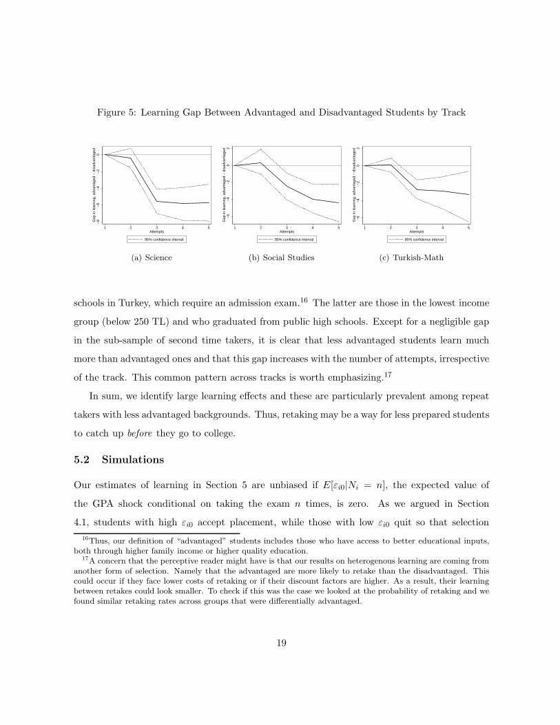
Figure 5: Learning Gap Between Advantaged and Disadvantaged Students by Track
−8
−6
−4
−2
0G
ap in
lear
ning
, adv
anta
ged
− d
isad
vant
aged
1 2 3 4 5Attempts
95% confidence interval
(a) Science
−6
−4
−2
02
Gap
in le
arni
ng, a
dvan
tage
d −
dis
adva
ntag
ed1 2 3 4 5
Attempts
95% confidence interval
(b) Social Studies
−6
−4
−2
02
Gap
in le
arni
ng, a
dvan
tage
d −
dis
adva
ntag
ed
1 2 3 4 5Attempts
95% confidence interval
(c) Turkish-Math
schools in Turkey, which require an admission exam.16 The latter are those in the lowest income
group (below 250 TL) and who graduated from public high schools. Except for a negligible gap
in the sub-sample of second time takers, it is clear that less advantaged students learn much
more than advantaged ones and that this gap increases with the number of attempts, irrespective
of the track. This common pattern across tracks is worth emphasizing.17
In sum, we identify large learning effects and these are particularly prevalent among repeat
takers with less advantaged backgrounds. Thus, retaking may be a way for less prepared students
to catch up before they go to college.
5.2 Simulations
Our estimates of learning in Section 5 are unbiased if E[εi0|Ni = n], the expected value of
the GPA shock conditional on taking the exam n times, is zero. As we argued in Section
4.1, students with high εi0 accept placement, while those with low εi0 quit so that selection
16Thus, our definition of “advantaged” students includes those who have access to better educational inputs,both through higher family income or higher quality education.
17A concern that the perceptive reader might have is that our results on heterogenous learning are coming fromanother form of selection. Namely that the advantaged are more likely to retake than the disadvantaged. Thiscould occur if they face lower costs of retaking or if their discount factors are higher. As a result, their learningbetween retakes could look smaller. To check if this was the case we looked at the probability of retaking and wefound similar retaking rates across groups that were differentially advantaged.
19

truncates the distribution of εi0 among retakers both from above and below. The truncation
from above makes E[εi0|Ni = n] negative which results in learning effects being overestimated
while truncation from below works in the opposite way. Truncation from above vanishes as
students get more patient. In this section, we use simulations to demonstrate that the bias
coming from ǫi0 tends to be small even when students are impatient.
We set up and simulate a dynamic decision model with the following structure:
1. A student is born with perfect knowledge of his GPA gi, ability θi, and all future learning
shocks Λin.
2. The student takes the entrance exam and learns his εin.
3. If the student’s score is above the placement threshold (120 points), he decides whether to
be placed. Placement is the terminal state; the utility from placement equals (si + ηgi).
4. If the student is below the threshold or chooses not to be placed, he learns the value of
quitting, V Qin = V Q0+ ξin, and chooses between quitting and retaking.18 Quitting is the
terminal state. Retaking is costly: (i) all retakers pay ψn before the next attempt, and
(ii) the value of retaking is discounted at a rate δ.
5. Steps 2–4 are repeated for students who choose to retake.
6. The option to retake disappears after the 10th attempt.19
In our simulations, for simplicity, students do not differ in observables Xi. We simulate GPA
and noise-free scores by independently drawing εi0, θi and λin from normal distributions with
parameters given in Table 3. We then substitute these draws into:
gi = E[gi|Ni = 1] + θi + εi0, sin = E[si1] + (ωqβq + ωvβv)θi +∑
k≤n
λik
18We need randomness in V Q in order to make the simulated number of retakers smooth in the model’sparameters. This makes it easier to calibrate the model. The shock ξin is drawn from the standard normaldistribution.
19We choose to shut down the option of retaking rather than extending the time periods indefinitely andassuming stationarity since most people stop retaking after three or four attempts. We do not expect our choicein this matter to affect our results.
20
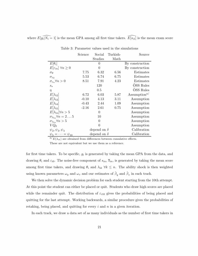
where E[gi|Ni = 1] is the mean GPA among all first time takers. E[si1] is the mean exam score
Table 3: Parameter values used in the simulations
Science Social Turkish- SourceStudies Math
E[θi] 0 By constructionE[εin] ∀n ≥ 0 0 By constructionσθ 7.75 6.32 6.56 Estimatesσε0 5.53 6.74 6.75 Estimatesσεn∀n > 0 8.51 7.91 4.23 Estimates
s∗ 120 OSS Rules
η 0.5 OSS Rules
E[λi2] 6.72 6.03 5.87 Assumptiona/
E[λi3] -0.10 4.13 3.11 AssumptionE[λi4] -0.43 2.44 1.09 AssumptionE[λi5] -2.16 2.61 0.75 AssumptionE[λin]∀n > 5 0 Assumptionσλin
∀n = 2 . . . 5 10 Assumptionσλin
∀n > 5 0 AssumptionV Q0 0 Assumptionψ2, ψ3, ψ4 depend on δ Calibrationψ5 = · · · = ψ10 depend on δ Calibrationa/E(λik) are obtained from differences between cumulative effects.
These are not equivalent but we use them as a reference.
for first time takers. To be specific, gi is generated by taking the mean GPA from the data, and
drawing θi and εi0. The noise-free component of sin, sin, is generated by taking the mean score
among first time takers, and drawing θi and λik ∀k ≤ n. The ability shock is then weighted
using known parameters ωq and ωv and our estimates of βq and βv in each track.
We then solve the dynamic decision problem for each student starting from the 10th attempt.
At this point the student can either be placed or quit. Students who draw high scores are placed
while the remainder quit. The distribution of εi10 gives the probabilities of being placed and
quitting for the last attempt. Working backwards, a similar procedure gives the probabilities of
retaking, being placed, and quitting for every i and n in a given iteration.
In each track, we draw a data set of as many individuals as the number of first time takers in
21

the actual data. Of course, individuals in the simulated data differ only in terms of their random
shocks and unobservables. We then calibrate ψn and V Q0 to target the number of repeat takers
in each attempt and the total number of quitters in early rounds in the actual data.20 After
calibrating the model, we use it to simulate 1000 artificial data sets and find the median bias
in our estimate of E[Λin|Ni = n] by track and number of attempts. Recall that the bias is
−(ωqβq +ωvβv)E[εi0|Ni = n]. We repeat this exercise for a range of discount factor values from
0.1 to 1. The 5th, 50th and 95th percentiles of the simulated bias are plotted in Figure 6.
The bias is affected by two forces that work against each other. On the one hand, students
with high εi0’s cash them in and get placed. This pushes E[ǫi0|Ni = n] down and upward biases
our learning estimates. On the other hand, quitting is more likely for students with low ǫi0’s.
This raises the average ǫi0 among repeat takers, making the learning bias negative. The former
effect is larger when students are impatient and thus the bias falls as δ rises. As explained
earlier, we expect no bias due to selection on ǫi0 from above when δ is close to one. If this is
true, our learning bias must be non-positive at δ = 1. This is clearly the case in the simulations.
Our simulations suggest the bias does exist, but its magnitude is substantially smaller than
any estimate of learning that we report in Tables 1 and 2. It is also worth noting that for
reasonable levels of patience (i.e., δ > 0.9) the bias in our learning estimates tends to be negative
so that we can think of them as a lower bound.
6 Conclusions and Proposed Agenda
Most people would agree that levelling the playing field in the educational arena is desirable. In
different settings, different approaches are taken with this objective in mind: minority prefer-
ences, quotas, remedial classes, scholarships, and so on. Preferential policies may however create
their own difficulties if admitted students fall further behind. Our work suggests that giving
second chances, without lowering standards, in an exam-based system may offer a way to help
the disadvantaged as they seem to learn more over attempts.
20We choose to match quitting patterns in attempts 1–3 as the terminal period becoming closer creates distor-tions in the simulated moments.
22

Figure 6: Simulated Bias in E(Λin|Ni = n) by Number of Attempts and Track
−2
−1
01
2P
oint
s
0 .2 .4 .6 .8 1δ
−2
−1
01
2P
oint
s
0 .2 .4 .6 .8 1δ
−2
−1
01
2P
oint
s
0 .2 .4 .6 .8 1δ
−2
−1
01
2P
oint
s
0 .2 .4 .6 .8 1δ
(a) Science
−2
−1
01
2P
oint
s
0 .2 .4 .6 .8 1δ
−2
−1
01
2P
oint
s
0 .2 .4 .6 .8 1δ
−2
−1
01
2P
oint
s
0 .2 .4 .6 .8 1δ
−2
−1
01
2P
oint
s
0 .2 .4 .6 .8 1δ
(b) Social Studies
−2
−1
01
2P
oint
s
0 .2 .4 .6 .8 1δ
−2
−1
01
2P
oint
s
0 .2 .4 .6 .8 1δ
−2
−1
01
2P
oint
s
0 .2 .4 .6 .8 1δ
−2
−1
01
2P
oint
s
0 .2 .4 .6 .8 1δ
Median 90% CI
(c) Turkish-Math
(a) n = 2 (b) n = 3 (c) n = 4 (d) n ≥ 5
23

One of the limitations of our paper is that we do not fully estimate the model outlined
in Section 4. Consequently, we cannot say much about what happens between attempts or
measure the net welfare impact of letting students retake the OSS and other counterfactuals.
We are currently working on a dynamic structural model that will allow us to measure marginal
learning as well as to evaluate the effects of different policy interventions such as setting a
maximum number of attempts. A second limitation is the known ability assumption. This is
still an open question that cannot be tackled with a cross-section data set. In this case, panel
data is required to disentangle learning about own ability and learning about the content of the
exam.
24
References
Arcidiacono, Peter, Esteban Aucejo, and Spenner Ken (2012) ‘What Happens After Enrollment?An Analysis of the Time Path of Racial Differences in GPA and Major Choice.’ IZA Journalof Labor Economics 5(1), 1–25.
Caner, Asena, and Cagla Okten (2010) ‘Risk and Career Choice: Evidence from Turkey.’ Eco-nomics of Education Review 29(6), 1060–1075.
(2013) ‘Higher education in Turkey: Subsidizing the rich or the poor?’ Economics of EducationReview 35, 75–92.
Card, David (2005) ‘Is the New Immigration Really so Bad?’ The Economic Journal115(506), F300–F323.
Carneiro, Pedro, Karsten Hansen, and James Heckman (2003) ‘Estimating Distributions ofTreatment Effects with an Application to the Returns to Schooling and Measurement of theEffects of Uncertainty on College.’ NBER Working Papers 9546
Cooley, Jane, Salvador Navarro, and Takahashi Yuya (2011) ‘How the Timing of Grade Re-tention Affects Outcomes: Identification and Estimation of Time-Varying Treatment Effects.’Working paper.
Frisancho, Veronica, and Kala Krishna (2012) ‘Affirmative Action in Higher Education in India:Targeting, Catch Up, and Mismatch.’ NBER Working Paper No. 17727.
Loury, Linda Datcher, and David Garman (1993) ‘Affirmative Action in Higher Education.’American Economic Review 83(2), 99–103.
(1995) ‘College Selectivity and Earnings.’ Journal of Labor Economics 13(2), 289–308. Uni-versity of Chicago Press.
Nathan, Julie, and Wayne Camara (1998) ‘Score Change When Retaking the SAT I: ReasoningTest.’ Research Notes, The College Board, Office of Research and Development.
Portes, Alejandro, and Ruben Rumbaut (2001) Legacies: The Story of the Immigrant SecondGeneration (Berkeley: University of California Press.)
Sander, Richard (2004) ‘A Systemic Analysis of Affirmative Action in American Law Schools.’Stanford Law Review 57(2), 367–483.
Saygin, Perihan (2011) ‘Gender Differences in College Applications: Evidence from the Central-ized System in Turkey.’ Working paper.
Tansel, Aysit, and Fatma Bircan (2005) ‘Effect of Private Tutoring on University EntranceExamination Performance in Turkey.’ IZA Discussion Paper, No. 1609.
Turk Egitim Dernegi (TED or Turkish Educational Association) (2005) ‘Study on the Univer-sity Placement System in Turkey and Suggestions for Solution.’ http://eua.cu.edu.tr/files/turkiyeninyuksekogretimstratejisi.pdf. The Council of Higher Education (YOK).
Vigdor, Jacob L., and Charles T. Clotfelter (2003) ‘Retaking the SAT.’ The Journal of HumanResources 38(1), 1–33.
25

A OSYM and the Higher Education Placement Process
The OSS tests student knowledge in four subjects: Mathematics, Turkish, Science, and SocialStudies.21 Each section of the exam is composed of 45 multiple choice questions which areworth one point for each correct answer and -0.25 for each incorrect answer. OSYM calculatesraw scores in each subject as well as two summary scores: raw verbal (raw Turkish and SocialStudies) and raw quantitative (raw Science and Math). These six raw scores are standardizedwith mean 50 and standard deviation 10. These standard scores are then used to construct threeweighted scores:
Weighted-Verbal = (1.8)*(Standard-Verbal) + (0.4)*(Standard-Quantitative),Weighted-Quantitative = (1.8)*(Standard-Quantitative) + (0.4)*(Standard-Verbal), andWeighted-Average = (0.8)*(Standard-Turkish + Standard-Math) + (0.3)*(Standard-Science
+ Standard-Social Studies ).For each weighted score exceeding 105 points, a placement score is calculated for the student:
Placement-Verbal, Placement-Quantitative, and Placement-Average. The placement scores areconstructed by adding the weighted standardized high school GPAs, denoted by “wsGPA”, tothe relevant weighted scores. The wsGPAs are constructed in a way to ensure that studentswill choose a field of study compatible with their high school track. As mentioned in Section3, the available tracks in most high schools are Science, Social Studies, and Turkish-Math. Therelevant scores for each of these tracks are Quantitative, Verbal and Average, respectively.
Calculating the wsGPAs is a complicated process. First, students’ GPAs are standardizedusing the GPA distribution in their high school to obtain sGPAs.22 For each student, threeweighted standardized GPAs (wsGPAV , wsGPAQ, and wsGPAA), one for each weighted score,are constructed according to the performance of the students’ high school in the relevant score.Finally, these wsGPAs are added with a weight of 0.5 when the placement score type matchesthe student’s high school track and a weight of 0.2 otherwise. For instance, placement scores fora Science track student are calculated as:
Placement-Verbal = Weighted-Verbal + (0.2)*wsGPAV
Placement-Quantitative = Weighted-Quantitative + (0.5)*wsGPAQ, andPlacement-Average = Weighted-Average + (0.2)*wsGPAA.Each field of study will assign seats to students on the basis of the relevant placement score.
For instance, a seat in a History program is based on Placement-Verbal score while a seat inan engineering program is rationed on the basis of Placement-Quantitative scores. Qualified
21There is also a Foreign Language Test (YDS), administered separately from the OSS. However, only studentswho are interested in careers that rely on the acquisition of a foreign language have to take this exam. In 2002,only around 40,000 students took this test. For that reason, we do not take the YDS into account in our analysis.
22Student i’s sGPA score is obtained in the following way:
sGPAi = 10
(
GPAi − µ
σ
)
+ 50
where µ and σ are the mean and standard deviation of raw GPAs in student i’s high school. sGPAs are calculatedthe first time a student takes the OSS, relative to the students graduating from his high school in that year, andthey are not updated over repeated attempts.
26

students can list up to 18 four-year programs on their preference lists in addition to 6 two-yearprograms. Before a student submits his placement preferences, he has access to all his scores,his percentiles for each score, and the previous year’s minimum and maximum scores for eachuniversity program.
B Standardized HS GPA versus quality normalized HS GPA
Raw and standardized GPAs ignore potential quality heterogeneity and grade inflation acrosshigh schools. Since we are interested in obtaining a measure that will allow us to rank studentson the same scale based on their high school academic performance, neither of these measuresare useful. Obtaining 10/10 at a very selective school is not the same as obtaining 10/10 at avery bad school.
To deal with this issue, we constructed school quality normalized GPAs. Within each trackk and for each school j, we define the adjustment factor, Ajk:
Ajk =GPAjk
Weighted Scorejk÷
GPAk
Weighted Scorek(B.1)
where GPAjk and Weighted Scorejk are the average GPA and weighted scores for each high
school and track combination. GPAk and Weighted Scorek are the average GPA and weightedscore across all comparable students from the same track.23 The numerator in (B.1) should goup if the school is inflating grades relative to its true quality. For example, if the average GPAin school j is about 8/10 but the average exam score for its students is only 5/10, school j isworse than the raw GPAs of its students suggest. After all, since the OSS is a standardizedexam, Weighted Scorejk should be a good proxy for the true quality of the school on a uniquescale. The denominator in (B.1) is just a constant for all the students in the same database andit takes the adjustment factor to a scale that is relative to everyone in the same track.
Define the school quality normalized GPA for student i in school j and track k as:
GPAnormijk = 100
(
GPAijk
GPAmax
k
)
where GPAijk is defined as:
GPAijk =
(
GPAijk
Ajk
)
and GPAmax
k is just the maximum GPAijk in a given k. Notice that if the student is in a schoolthat tends to inflate the grades relative to true performance, the raw GPA of all the students insuch a school will be penalized through a higher Ajk.
23This adjustment factor is constructed using weighted quantitative scores for Science students while SocialStudies students’ factor relies on weighted verbal scores. For Turkish-Math students, we use the weighted average.
27

C Additional Tables and Figures
Table C.1: Descriptive Statistics
Science Social Studies Turkish-MathVariable Mean S.D. Mean S.D. Mean S.D.
Individual and Family Background
Gender 0.59 0.57 0.51Raw HS GPA 68.19 15.77 57.28 10.64 63.16 13.41Standardized HS GPA 51.68 10.01 47.66 7.78 48.99 8.89School TypePublic 0.59 0.86 0.71Private 0.18 0.02 0.14Anatolian/Science 0.20 0.02 0.11Other 0.03 0.09 0.05
Father’s educationPrimary or less 0.39 0.56 0.44Middle/High school 0.30 0.28 0.332-year higher education 0.06 0.03 0.04College/Master/PhD 0.17 0.05 0.11Missing 0.08 0.08 0.09
More than 3 children in the household 0.38 0.49 0.39Household Monthly Income<250TL 0.34 0.45 0.37[250− 500]TL 0.40 0.38 0.40>500TL 0.26 0.17 0.23
Preparation for the Exam
Student was working when exam was taken 0.13 0.21 0.10Prep school/tutoring expendituresDid not attend Prep school 0.13 0.26 0.19Scholarship 0.04 0.01 0.01<1b TL 0.35 0.22 0.31[1− 2]b TL 0.20 0.09 0.17>2b TL 0.10 0.03 0.08Missing 0.17 0.38 0.23
Exam Performance
Took language exam 0.01 0.01 0.01Weighted score 124.02 29.99 113.53 26.61 113.48 20.82Number of attempts1st attempt 0.42 0.25 0.462nd attempt 0.25 0.25 0.303rd attempt 0.16 0.25 0.164th attempt 0.09 0.16 0.065th attempt 0.07 0.10 0.02
Student was placed 0.36 0.23 0.26
28

Table C.2: Estimates of [α0, α1, α2] by Track
Science Social Studies Turkish-MathGPA sq sv GPA sq sv GPA sq sv
Constant 49.798 4.406 14.301 52.285 -1.777 27.041 53.79 20.762 9.011(1.198) (2.240) (2.074) (1.597) (0.564) (2.733) (1.111) (1.558) (1.072)
Male -2.611 6.191 -2.423 -3.208 0.067 -1.07 -4.692 -1.631 0.075(0.160) (0.299) (0.276) (0.205) (0.072) (0.351) (0.153) (0.215) (0.148)
Student was working when exam was taken -1.798 -4.21 -2.309 -1.112 -0.143 -2.875 -1.666 -2.473 -1.352(0.465) (0.871) (0.806) (0.324) (0.115) (0.555) (0.376) (0.528) (0.363)
School Type (base: Public)Private 5.206 13.031 7.143 10.187 2.499 16.639 5.458 13.052 7.312
(0.401) (0.749) (0.694) (1.291) (0.456) (2.209) (0.409) (0.574) (0.395)Anatolian/Science 11.033 25.206 17.133 9.09 3.814 21.204 7.692 19.487 11.284
(0.370) (0.693) (0.641) (0.757) (0.268) (1.295) (0.374) (0.525) (0.361)Other -0.473 -1.687 2.122 0.077 0.006 -1.133 -0.526 0.548 0.437
(0.672) (1.256) (1.163) (0.404) (0.143) (0.691) (0.493) (0.692) (0.476)Household Monthly Income (base: <250TL)
[250500]TL -0.437 -1.172 -0.68 -0.676 -0.093 -0.453 -0.649 -1.104 -0.604(0.287) (0.538) (0.498) (0.258) (0.091) (0.442) (0.226) (0.317) (0.218)
>500TL -1.492 -2.106 -0.353 -1.043 -0.624 -1.429 -1.996 -2.617 -1.752(0.392) (0.733) (0.679) (0.378) (0.133) (0.646) (0.320) (0.449) (0.309)
School Type x HH Monthly IncomePrivate x [250500]TL -0.214 -0.809 1.13 1.026 -0.287 -1.006 0.873 0.859 0.006
(0.506) (0.946) (0.876) (1.662) (0.588) (2.845) (0.518) (0.727) (0.501)Private x >500TL 1.294 -0.977 2.771 -0.868 0.042 -3.722 0.983 0.798 -0.074
(0.571) (1.068) (0.988) (1.561) (0.552) (2.671) (0.559) (0.785) (0.540)Anatolian/Science x [250500]TL 1.348 1.469 3.406 2.166 1.074 -0.344 1.235 1.25 0.656
(0.455) (0.850) (0.787) (1.061) (0.375) (1.816) (0.475) (0.666) (0.458)Anatolian/Science x >500TL 2.627 2.57 3.203 2.085 5.466 -1.128 3.39 3.581 1.978
(0.518) (0.968) (0.896) (1.264) (0.447) (2.164) (0.530) (0.744) (0.512)Other x [250500]TL 1.437 3.81 4.174 0.329 0.149 1.246 0.012 0.527 -0.138
(0.932) (1.744) (1.615) (0.604) (0.214) (1.035) (0.774) (1.086) (0.747)Other x >500TL 2.134 5.876 8.237 -0.09 0.52 1.733 1.08 0.253 1.494
(1.408) (2.634) (2.438) (0.798) (0.282) (1.365) (1.162) (1.631) (1.122)Expenditures in dersanes (base: Did not attend)
Scholarship 12.367 28.789 20.657 7.698 2.227 15.819 8.182 15.212 10.053(0.439) (0.822) (0.760) (1.063) (0.376) (1.819) (0.606) (0.850) (0.585)
<1b TL 4.256 14.04 4.607 3.335 1.021 10.748 3.12 9.209 4.973(0.276) (0.516) (0.477) (0.286) (0.101) (0.490) (0.217) (0.305) (0.210)
Continues on next page...
29

... continued from previous page
Science Social Studies Turkish-MathGPA sq sv GPA sq sv GPA sq sv
[1− 2]b TL 2.801 11.842 2.384 3.157 1.537 12.218 3.417 10.871 5.642(0.314) (0.587) (0.543) (0.452) (0.160) (0.773) (0.274) (0.385) (0.265)
>2b TL 2.887 12.503 3.656 4.13 4.328 14.227 3.666 12.608 6.737(0.384) (0.719) (0.666) (0.852) (0.301) (1.459) (0.378) (0.531) (0.365)
Missing -0.381 0.735 0.789 -0.386 0.017 -0.74 -0.674 -0.322 -0.318(0.334) (0.625) (0.578) (0.235) (0.083) (0.402) (0.234) (0.329) (0.226)
Father’s occupation (base: Employer)Works for wages/salary 1.552 3.044 2.184 1.778 0.659 2.614 0.91 1.113 0.7
(0.391) (0.732) (0.677) (0.610) (0.216) (1.044) (0.370) (0.519) (0.357)Self-employed 1.332 2.823 1.907 1.711 0.608 2.585 0.891 0.851 0.431
(0.407) (0.762) (0.705) (0.619) (0.219) (1.060) (0.380) (0.533) (0.367)Unemployed/not in Labor Force 1.123 2.78 2.016 1.697 0.584 1.723 1.114 1.112 0.7
(0.467) (0.873) (0.808) (0.655) (0.231) (1.121) (0.432) (0.606) (0.417)Mother’s occupation (base: Employer)
Works for wages/salary 2.528 2.441 2.86 1.167 1.144 0.356 1.345 0.282 1.494(1.092) (2.042) (1.890) (1.502) (0.531) (2.571) (1.030) (1.446) (0.995)
Self-employed 2.649 3.108 2.286 1.531 1.483 0.116 2.363 0.397 2.087(1.145) (2.141) (1.982) (1.516) (0.536) (2.595) (1.068) (1.499) (1.032)
Unemployed/not in Labor Force 2.961 3.038 3.594 1.008 1.39 -0.426 2.273 1.064 1.84(1.077) (2.015) (1.865) (1.469) (0.519) (2.514) (1.012) (1.420) (0.977)
Father’s education (base: Primary or less)Middle/High school -0.051 0.198 0.22 -0.387 0.091 0.064 -0.143 0.133 0.19
(0.215) (0.402) (0.372) (0.247) (0.087) (0.423) (0.191) (0.268) (0.184)2-year higher education 0.982 2.34 1.317 -0.344 -0.532 -1.23 0.784 0.836 0.312
(0.364) (0.680) (0.629) (0.677) (0.239) (1.159) (0.399) (0.560) (0.386)College/Master/PhD 1.829 4.075 3.515 1.316 0.488 2.956 1.329 2.462 1.839
(0.292) (0.547) (0.506) (0.544) (0.192) (0.931) (0.311) (0.436) (0.300)Missing -0.098 -0.091 -1.114 -0.343 -0.3 -0.658 0.392 0.009 -0.586
(0.535) (1.001) (0.927) (0.580) (0.205) (0.993) (0.464) (0.652) (0.448)Mother’s education (base: Primary or less)
Middle/High school -0.862 -1.527 0.024 -1.249 -0.023 -0.867 -0.468 0.57 -0.181(0.227) (0.425) (0.394) (0.336) (0.119) (0.575) (0.229) (0.321) (0.221)
2-year higher education 0.725 0.913 2.396 0.11 2.025 1.462 1.137 2.582 1.584(0.450) (0.842) (0.779) (1.169) (0.413) (2.001) (0.549) (0.771) (0.530)
College/Master/PhD 1.144 1.624 3.401 -0.875 2.715 2.446 1.666 3.959 2.136(0.415) (0.777) (0.719) (1.009) (0.356) (1.726) (0.491) (0.689) (0.474)
Continues on next page...
30

... continued from previous page
Science Social Studies Turkish-MathGPA sq sv GPA sq sv GPA sq sv
Missing 0.027 -0.003 1.281 -0.65 0.193 -0.676 -0.744 -0.075 0.549(0.583) (1.090) (1.009) (0.692) (0.245) (1.185) (0.526) (0.738) (0.508)
More than 3 children in the household -0.042 -0.535 -1.543 -0.125 -0.027 -1.331 0.358 -0.619 -0.02(0.194) (0.364) (0.337) (0.213) (0.075) (0.365) (0.173) (0.243) (0.167)
Internet access (base: No internet access)At home -0.476 -0.772 -1.424 0.437 -0.037 0.576 -0.458 -1.26 -0.049
(0.249) (0.466) (0.431) (0.482) (0.170) (0.825) (0.288) (0.404) (0.278)Not at home -0.009 -0.793 -2.945 1.233 -0.164 0.706 0.389 -1.143 -0.249
(0.253) (0.474) (0.438) (0.468) (0.165) (0.801) (0.286) (0.402) (0.277)Missing -1.267 -2.914 -4.648 0.468 -0.213 -0.831 -0.743 -3.005 -0.769
(0.496) (0.927) (0.858) (0.609) (0.215) (1.042) (0.452) (0.635) (0.437)Population in Town of HS (base: Over a million)
<10,000 -1.458 0.857 -0.962 -1.135 -0.055 1.646 -1.999 -0.704 -0.516(0.389) (0.727) (0.673) (0.360) (0.127) (0.617) (0.323) (0.453) (0.312)
[10, 000− 50, 000] -0.66 4.59 3.058 -1.199 0.263 2.827 -1.93 1.746 0.935(0.370) (0.693) (0.641) (0.353) (0.125) (0.604) (0.314) (0.441) (0.303)
[50, 000− 250, 000] -0.568 4.657 3.177 -1.289 0.212 2.62 -1.761 1.716 0.682(0.386) (0.722) (0.669) (0.392) (0.139) (0.672) (0.336) (0.471) (0.324)
[250, 000− 1, 000, 000] 0.362 6.82 6.566 -0.578 0.577 3.742 -0.836 3.53 2.446(0.364) (0.680) (0.630) (0.345) (0.122) (0.591) (0.310) (0.435) (0.300)
Missing -1.83 1.82 1.34 -1.929 -0.081 0.125 -3.501 -0.843 -0.254(0.456) (0.853) (0.789) (0.387) (0.137) (0.662) (0.370) (0.519) (0.357)
Funds to Pay for College (base: Family funds)Student’s work -1.007 -1.698 -1.246 0.089 0.099 0.103 -0.132 0.515 0.561
(0.216) (0.403) (0.373) (0.249) (0.088) (0.426) (0.197) (0.276) (0.190)Loan 0.147 0.867 -0.965 0.664 0.237 1.691 0.671 1.393 0.738
(0.182) (0.341) (0.315) (0.263) (0.093) (0.450) (0.183) (0.256) (0.176)Other -1.384 -1.555 -1.407 -0.266 0.143 0.83 -0.389 -0.087 -0.024
(0.360) (0.673) (0.623) (0.388) (0.137) (0.664) (0.328) (0.460) (0.316)
Observations 15,587 15,587 15,587 9,012 9,012 9,012 16,457 16,457 16,457R-squared 0.369 0.473 0.366 0.166 0.251 0.255 0.271 0.487 0.378
31

Table C.3: Estimates of Factor Variances and Loadings
Science Social Studies Turkish-Math
βq 1.146 2.056 1.028
(0.020) (0.112) (0.013)
βv 1.938 0.155 1.815(0.028) (0.008) (0.022)
σ2θ 60.023 39.883 43.035(1.186) (2.451) (0.936)
σ2ǫ0 30.575 45.362 45.619(0.970) (2.354) (0.826)
ˆσ2ǫ1q 91.559 9.686 32.685
(3.140) (0.547) (1.337)
ˆσ2ǫ1v 192.851 81.176 37.157(2.344) (8.839) (0.666)
ωq 0.844 0.187 0.670(0.000) (0.000) (0.000)
ωv 0.195 0.876 0.293(0.000) (0.000) (0.000)
Observations 15,587 9,012 16,457
32