1

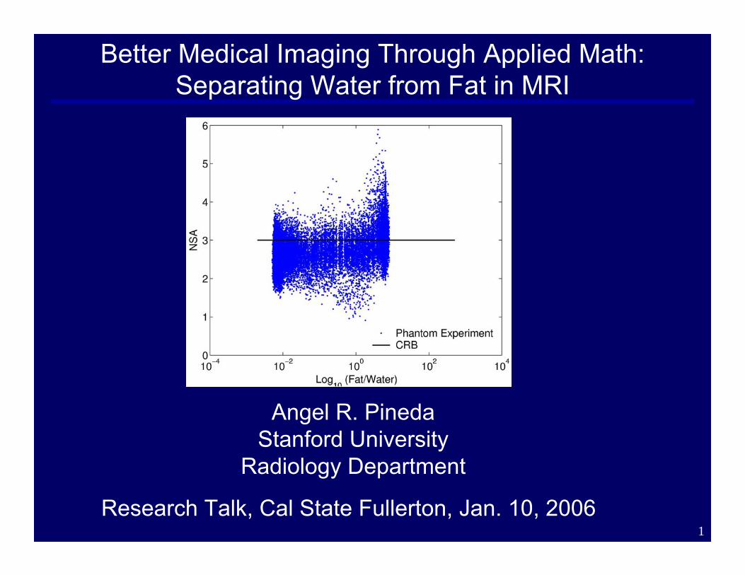
Better Medical Imaging Through Applied Math:Separating Water from Fat in MRI

Angel R. PinedaStanford University

Radiology Department

Research Talk, Cal State Fullerton, Jan. 10, 2006

2

Acknowledgments (much abridged)

Zhifei Wen (Stanford, now UW Madison)

Huanzhou Yu (Stanford, now GE Healthcare)

Jean Brittain (GE Healthcare)

Scott Reeder (Stanford, now UW Madison)

Norbert Pelc (Stanford)

Brian Hargreaves (Stanford)

3

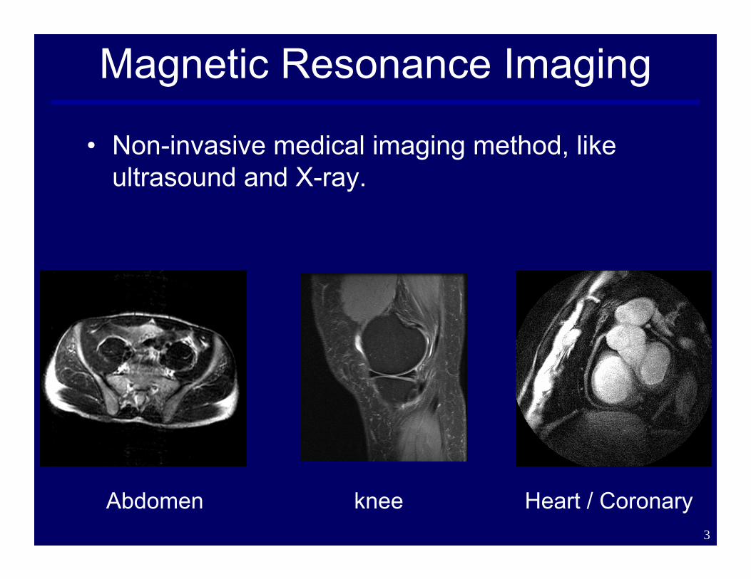
Magnetic Resonance Imaging

• Non-invasive medical imaging method, like ultrasound and X-ray.

Abdomen knee Heart / Coronary

4

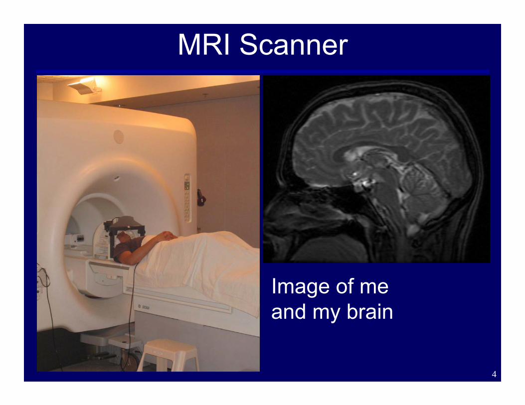
MRI Scanner

Image of me and my brain

5

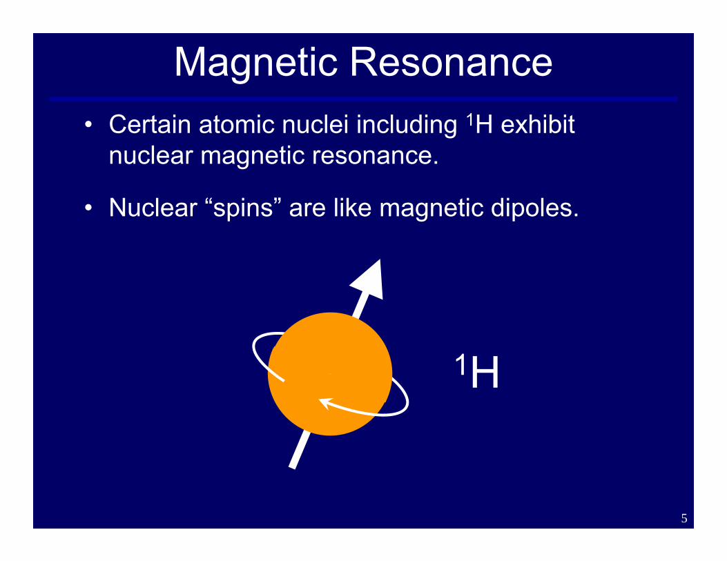
Magnetic Resonance• Certain atomic nuclei including 1H exhibit

nuclear magnetic resonance.

• Nuclear “spins” are like magnetic dipoles.

1H

6

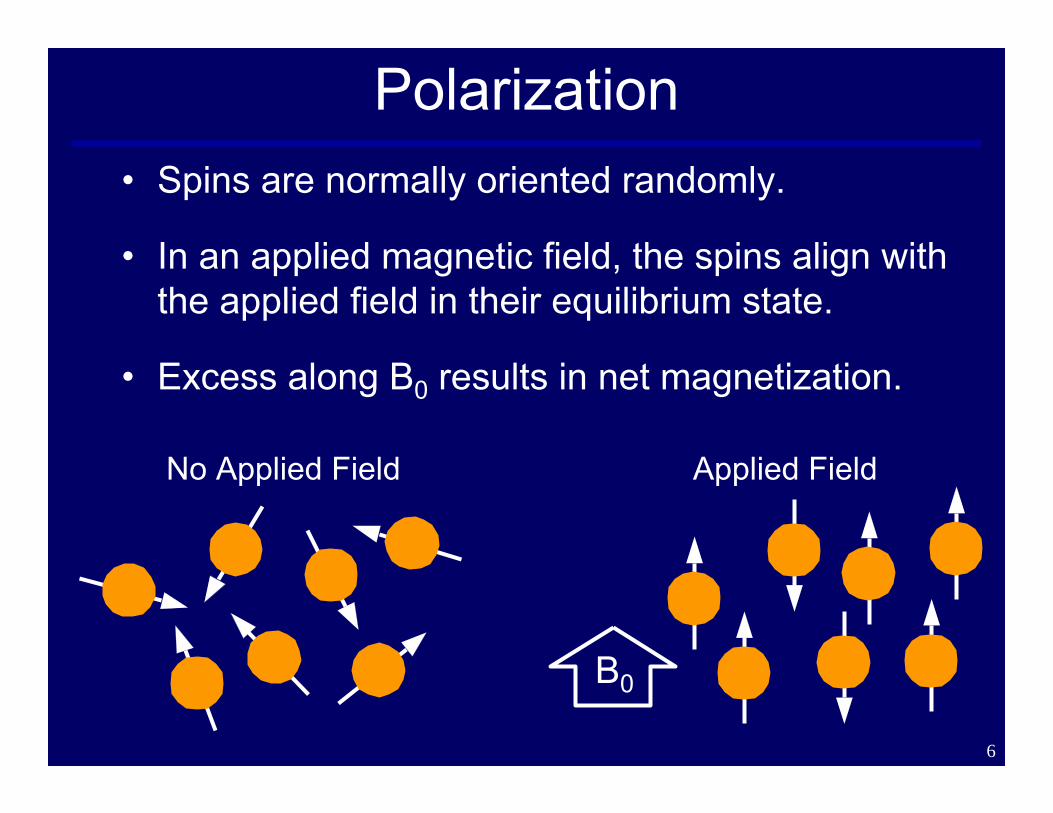
Polarization• Spins are normally oriented randomly.

• In an applied magnetic field, the spins align with the applied field in their equilibrium state.

• Excess along B0 results in net magnetization.

No Applied Field Applied Field

B0

7

Static Magnetic Field

Longitudinal

Transverse

B0

z

x, y

8

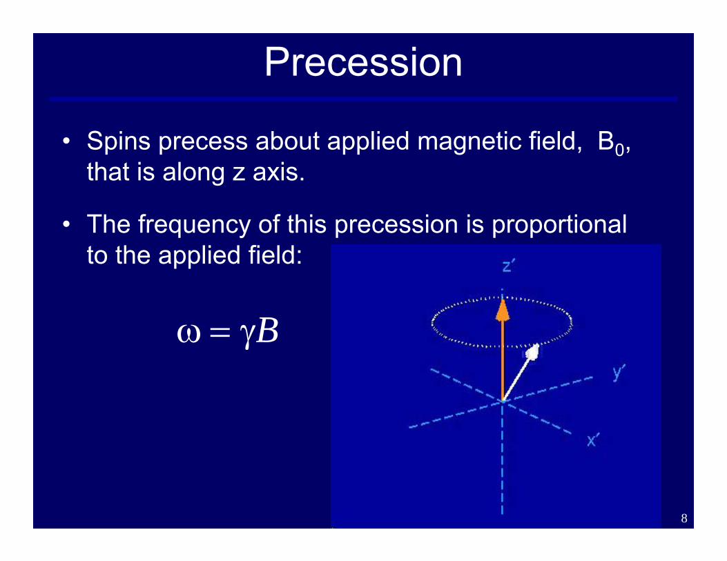
Precession

• Spins precess about applied magnetic field, B0, that is along z axis.

• The frequency of this precession is proportional to the applied field:

Bγ=ω

9

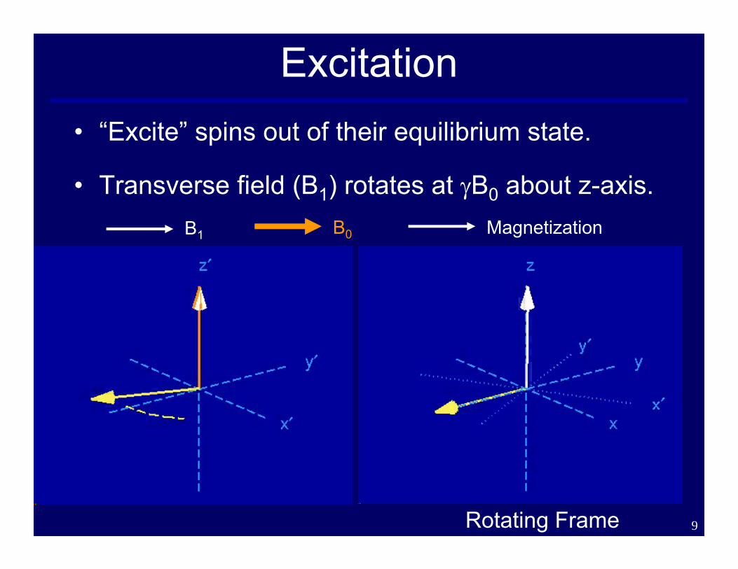
Excitation• “Excite” spins out of their equilibrium state.

• Transverse field (B1) rotates at γB0 about z-axis.B1 MagnetizationB0

Rotating Frame

10

Signal Reception• Precessing spins cause a change in flux (Φ) in

a transverse receive coil.

• Flux change induces a voltage across the coil with two orthogonal coils, one obtains a complex measurement.

Signal

y

x

B0

z

Φ

11

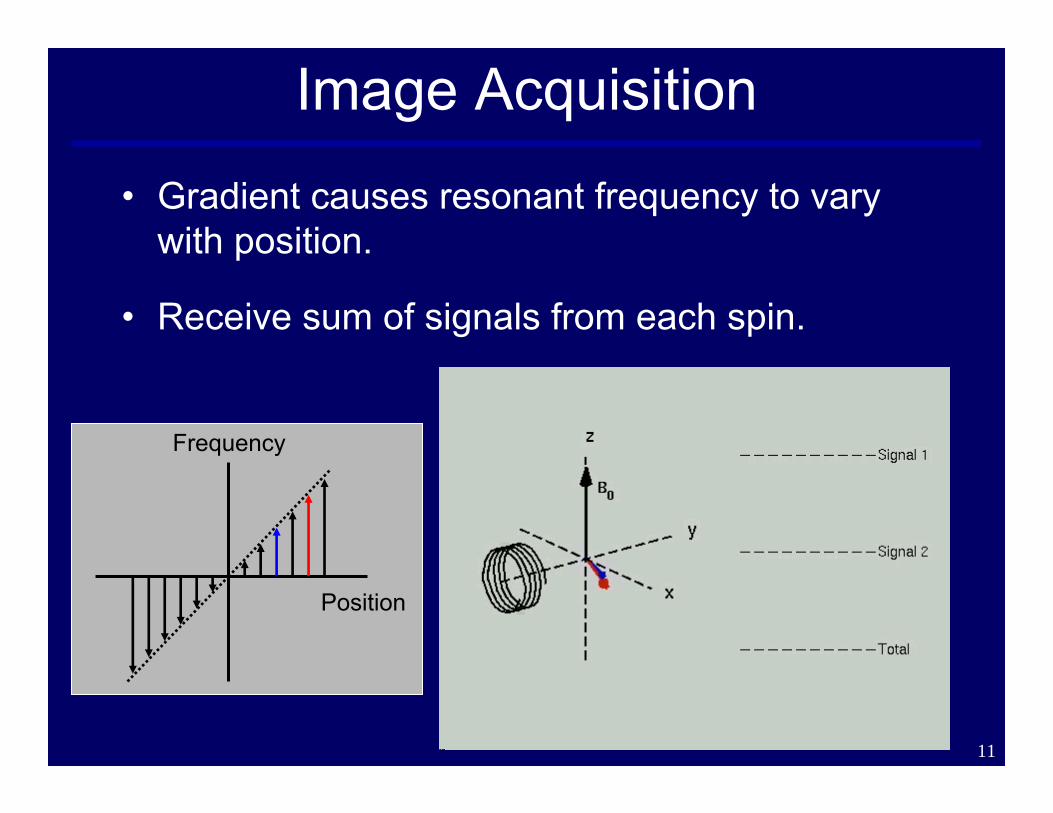
Image Acquisition

• Gradient causes resonant frequency to vary with position.

• Receive sum of signals from each spin.

Frequency

Position

12

Image Reconstruction

• Received signal is a sum of “tones.”

• The “tones” of the signal are the image.

• This also applies to 2D and 3D images.

InverseFourier

Transform

Received SignalImage

13

Off-Resonance effects

• The magnetic field strength is not perfectly uniform and tissue is made up of multiple chemical species.

• Resonant frequency is proportional to field and the gyromagnetic ratio:

z

y

x

z

y

x

Bω γ∝

0ω−ω=ωΔOff-resonance:

14

Spin Echoes

• 180° rotation can reverse the dephasing effects of off-resonance by flipping the spins about the x-axis.

• Spins realign at some time to form a spin echo

15

Separating Chemical SpeciesSpin Echo

TE1

TE2

TE3

Excitation

--- time axis --- (TE=0 at the Spin Echo)

16

Motivation: Artifacts due to Fat

Water Image Failed Fat Saturation

17

Problem Summary

• Tissue is primarily composed of water and fat.

• Diagnostic information is in the water signal.

• The fat signal obscures underlying pathology.

• In the presence of field inhomogeneities and measurement noise, what is the choice of TE’sthat allow us to best estimate water and fat?

18

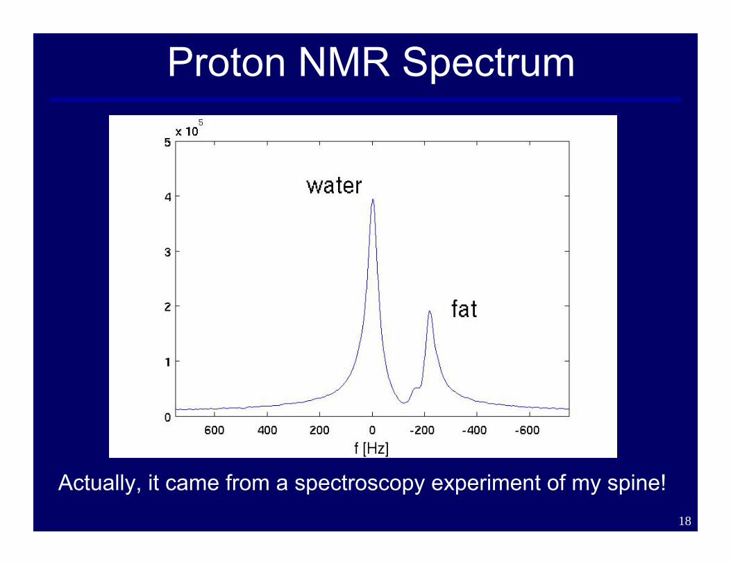
Proton NMR Spectrum

Actually, it came from a spectroscopy experiment of my spine!

19

The “Dixon” Model

20

Evolution of the Mathematical Model

• 2-Point Dixon (assumes uniform magnetic field)

• 3-Point Dixon (estimates field inhomogeneity (ψ) along with water and fat)

• We are trying to propagate the uncertainty in ψ to the water and fat estimates in the 3-Point Dixon model

21

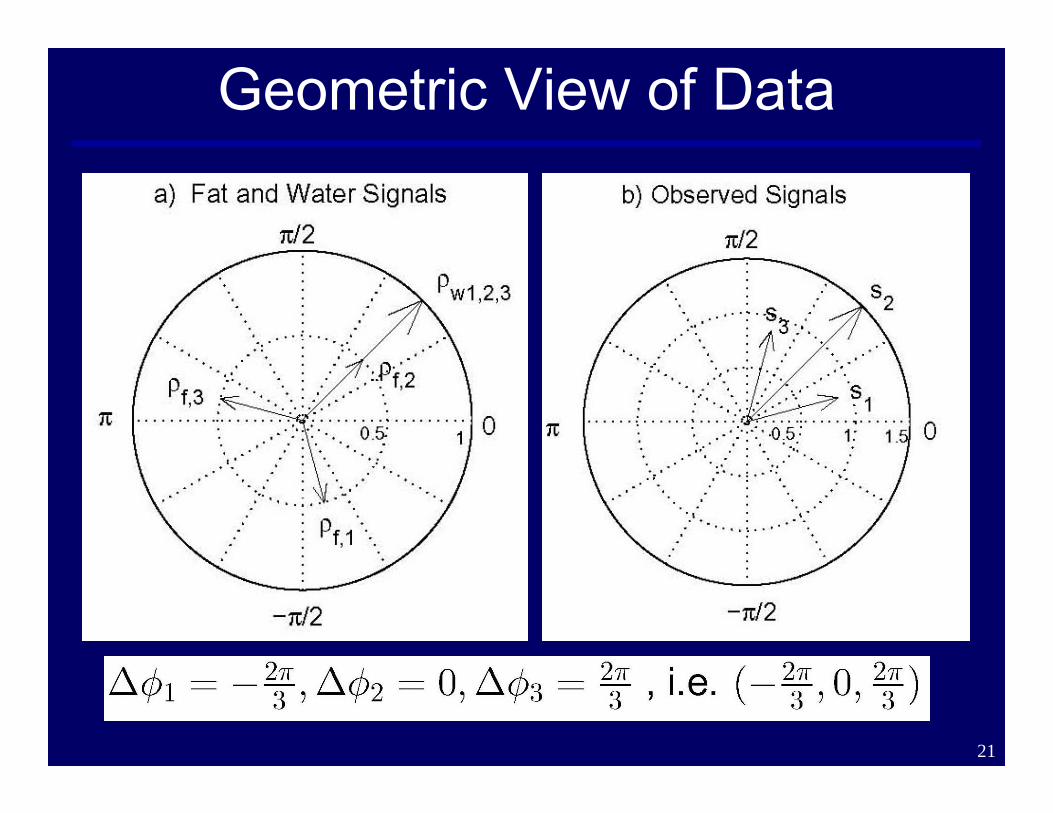
Geometric View of Data

22

Fisher Information Matrix

23

Fisher Information Matrix

24

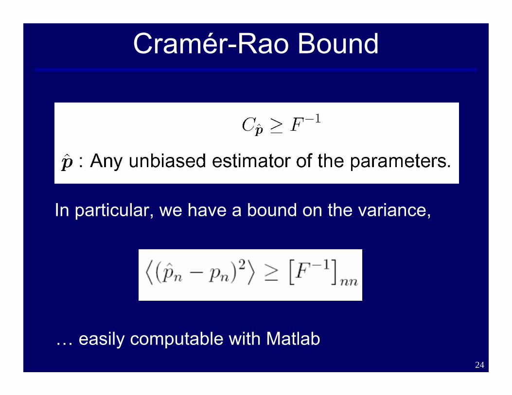
Cramér-Rao Bound

… easily computable with Matlab

In particular, we have a bound on the variance,

25

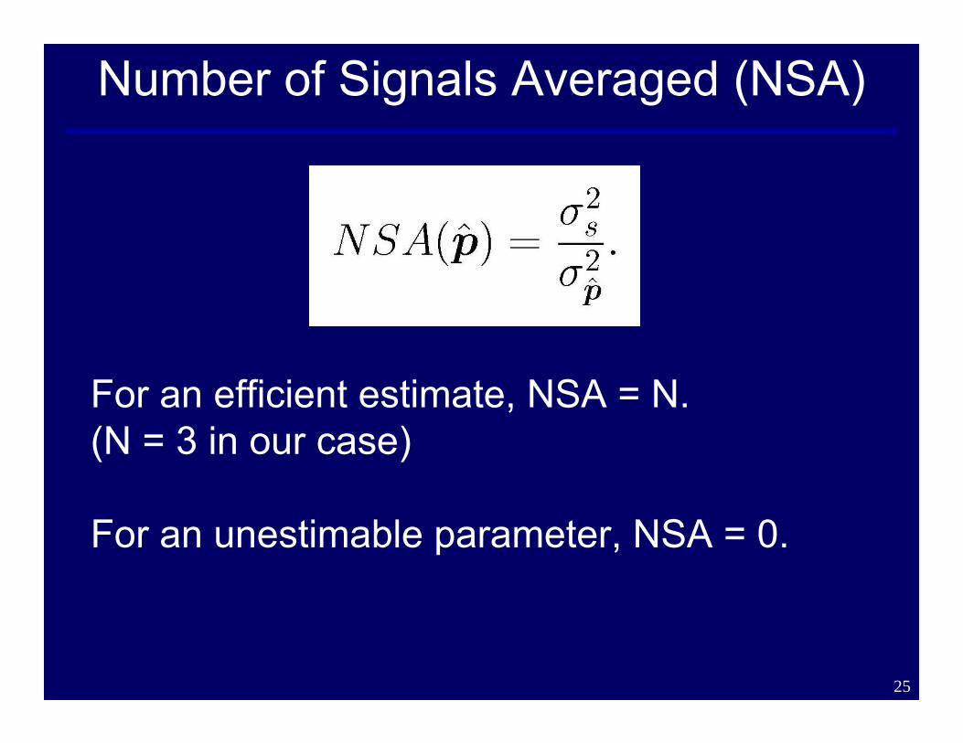
Number of Signals Averaged (NSA)

For an efficient estimate, NSA = N.(N = 3 in our case)

For an unestimable parameter, NSA = 0.

26

Generalizing the NSA…

27

Factors that affect the NSA

• Choice of echo time shifts

• Phase of water and fat at echo

• Chemical composition of the pixel

28

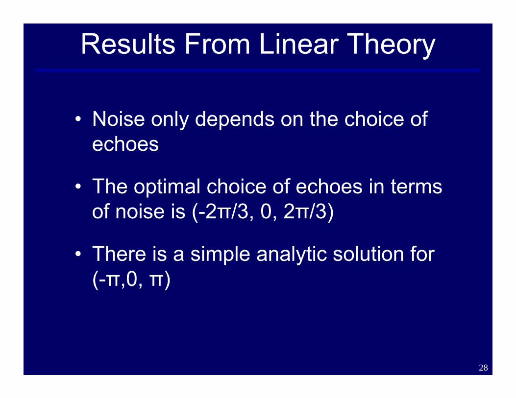
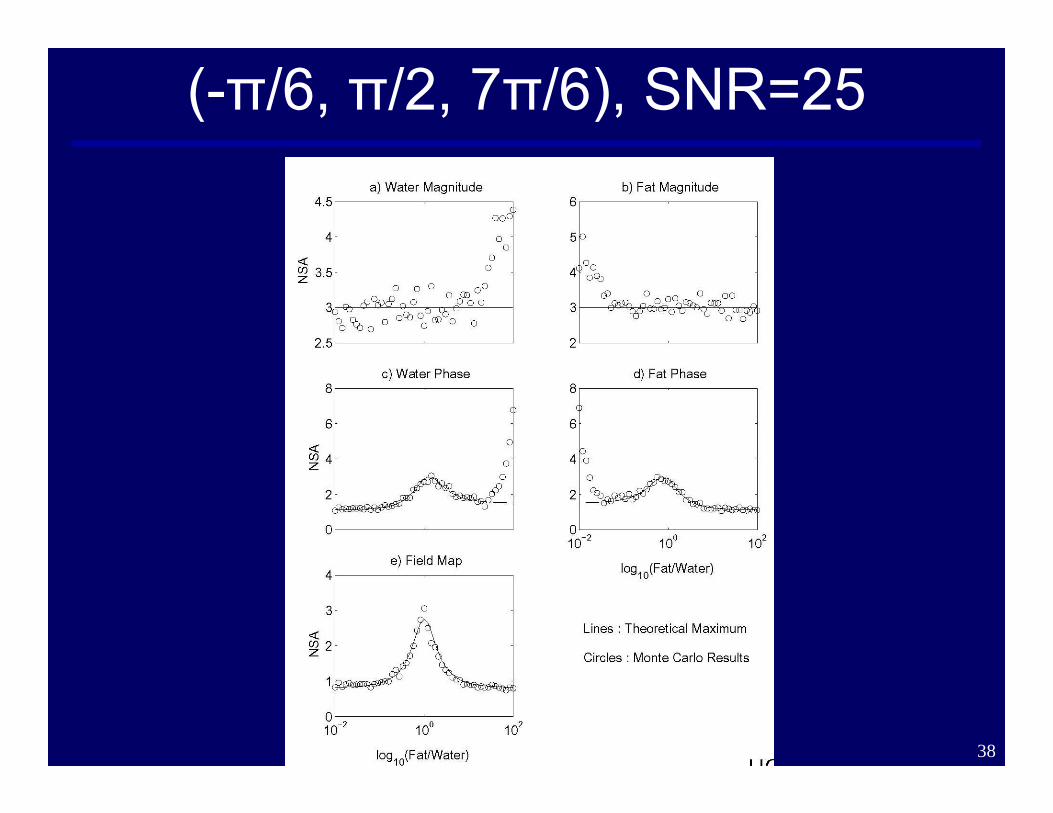
Results From Linear Theory

• Noise only depends on the choice of echoes

• The optimal choice of echoes in terms of noise is (-2π/3, 0, 2π/3)

• There is a simple analytic solution for (-π,0, π)

29

Linear Results

• CRB for magnitude

• Estimation Using Pseudo-Inverse (Maximum Likelihood Estimator (MLE))

• Monte Carlo simulations with (Signal-to-Noise Ratio (SNR) = 200)

30

(-2π/3, 0, 2π/3), Linear Results (ψ=0)

31

(-π, 0, π), Linear Results (ψ=0)

32

Revisiting Linear Results

• CRB for all unknowns

• Iterative algorithm for estimation (Maximum Likelihood Estimator (MLE))

• Monte Carlo simulations with (Signal-to-Noise Ratio (SNR) = 200)

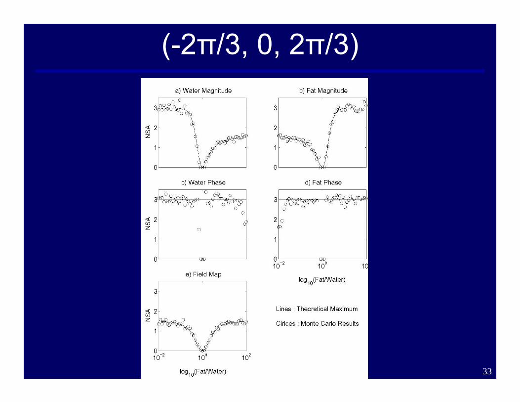
33

(-2π/3, 0, 2π/3)

34

(-π, 0, π)

35

Butterfly Plot

36

(-π/6, π/2, 7π/6)

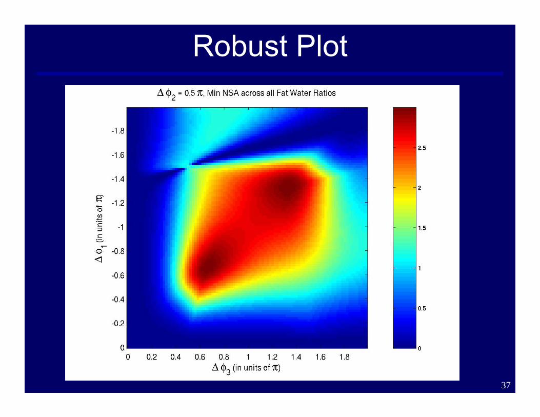
37

Robust Plot

38

(-π/6, π/2, 7π/6), SNR=25

39

Experimental Verification

Source Water Fat

40

Symmetric Echoes

41

Asymmetric Echoes

42

Theory and the Clinic Come Together!

Symmetric Acquisition Asymmetric Acquisition

43

Conclusions• CRB leads to an ideal solution

• The iterative algorithm achieves the CRB

• Generalization of NSA for nonlinear parameters

• Better understanding of the factors that affect the noise

• Iterative Decomposition of water and fat with Echo Asymmetry and Least squares estimation (IDEAL)

44

Future Work

• On the theory…

• Prior information and regularization, improving the model to account for more realistic biology and physics

• On the application…

• Parallel imaging

• Hyperpolarized C-13 imaging of metabolic function

45

Thank you for your time…