Full Terms & Conditions of access and use can be found athttp://www.tandfonline.com/action/journalInformation?journalCode=lsta20

Download by: [Arkansas State University] Date: 17 September 2015, At: 14:04

Communications in Statistics - Theory and Methods

ISSN: 0361-0926 (Print) 1532-415X (Online) Journal homepage: http://www.tandfonline.com/loi/lsta20

Bounded Area Tests For Comparing The DynamicsBetween ARMA Processes

Ferebee Tunno

To cite this article: Ferebee Tunno (2015) Bounded Area Tests For Comparing The DynamicsBetween ARMA Processes, Communications in Statistics - Theory and Methods, 44:18,3921-3941, DOI: 10.1080/03610926.2013.837184

To link to this article: http://dx.doi.org/10.1080/03610926.2013.837184

Accepted online: 01 Apr 2015.

Submit your article to this journal

Article views: 6

View related articles

View Crossmark data

Communications in Statistics—Theory and Methods, 44: 3921–3941, 2015Copyright © Taylor & Francis Group, LLCISSN: 0361-0926 print / 1532-415X onlineDOI: 10.1080/03610926.2013.837184

Bounded Area Tests For Comparing The DynamicsBetween ARMA Processes

FEREBEE TUNNO

Arkansas State University, Department of Mathematics and Statistics,State University, Arkansas, USA

This article presents a new test for discerning whether or not two independent autore-gressive moving average (ARMA) processes have the same autocovariance structure.This test utilizes a specific geometric feature of a time series plot, namely the areabounded between the line segments that connect adjacent points and the time axis. Itwill be shown that if you sample two ARMA processes and calculate the magnitudes ofthe two resulting bounded areas, then a significant difference among these areas tendsto imply a significant difference in autocovariances.

Keywords Bounded area; Autocovariance; ARMA.

Mathematics Subject Classification Primary 62M10; Secondary 60G10.

1. Introduction

Consider the causal stationary ARMA(p, q) time series {Xt } defined by

Xt −p∑i=1

φiXt−i = εt +q∑j=1

θj εt−j t = 0,±1,±2, . . . , (1.1)

where E(Xt ) = 0, E(X2t ) < ∞, {εt } ∼ IID(0, σ 2), and the roots of φ(z) = 1 − φ1z− · · · −

φpzp fall outside the unit circle. {Xt } then has a linear process representation given by

Xt =∞∑j=0

ψjεt−j ,

where the ψj ’s are absolutely summable, and an autocovariance function given by

γX(h) = Cov(Xt,Xt+h) = σ 2∞∑j=0

ψjψj+h h = 0, 1, 2, . . . .

Received March 15, 2013; Accepted August 19, 2013.Address correspondence to Ferebee Tunno, Department of Mathematics and Statistics, Arkansas

State University, P.O. Box 70, State University, Arkansas; E-mail: ftunno@astate.edu

3921

Dow

nloa

ded

by [

Ark

ansa

s St

ate

Uni

vers

ity]

at 1

4:04

17

Sept

embe

r 20

15

3922 Tunno

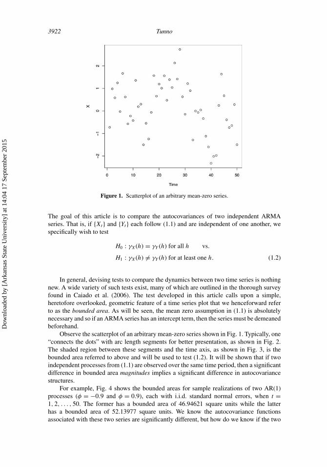
Figure 1. Scatterplot of an arbitrary mean-zero series.

The goal of this article is to compare the autocovariances of two independent ARMAseries. That is, if {Xt } and {Yt } each follow (1.1) and are independent of one another, wespecifically wish to test

H0 : γX(h) = γY (h) for all h vs.

H1 : γX(h) �= γY (h) for at least one h. (1.2)

In general, devising tests to compare the dynamics between two time series is nothingnew. A wide variety of such tests exist, many of which are outlined in the thorough surveyfound in Caiado et al. (2006). The test developed in this article calls upon a simple,heretofore overlooked, geometric feature of a time series plot that we henceforward referto as the bounded area. As will be seen, the mean zero assumption in (1.1) is absolutelynecessary and so if an ARMA series has an intercept term, then the series must be demeanedbeforehand.

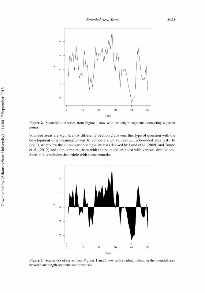
Observe the scatterplot of an arbitrary mean-zero series shown in Fig. 1. Typically, one“connects the dots” with arc length segments for better presentation, as shown in Fig. 2.The shaded region between these segments and the time axis, as shown in Fig. 3, is thebounded area referred to above and will be used to test (1.2). It will be shown that if twoindependent processes from (1.1) are observed over the same time period, then a significantdifference in bounded area magnitudes implies a significant difference in autocovariancestructures.

For example, Fig. 4 shows the bounded areas for sample realizations of two AR(1)processes (φ = −0.9 and φ = 0.9), each with i.i.d. standard normal errors, when t =1, 2, . . . , 50. The former has a bounded area of 46.94621 square units while the latterhas a bounded area of 52.13977 square units. We know the autocovariance functionsassociated with these two series are significantly different, but how do we know if the two

Dow

nloa

ded

by [

Ark

ansa

s St

ate

Uni

vers

ity]

at 1

4:04

17

Sept

embe

r 20

15

Bounded Area Tests 3923

Figure 2. Scatterplot of series from Figure 1 now with arc length segments connecting adjacentpoints.

bounded areas are significantly different? Section 2 answers this type of question with thedevelopment of a meaningful way to compare such values (i.e., a bounded area test). InSec. 3, we review the autocovariance equality tests devised by Lund et al. (2009) and Tunnoet al. (2012) and then compare them with the bounded area test with various simulations.Section 4 concludes the article with some remarks.

Figure 3. Scatterplot of series from Figures 1 and 2 now with shading indicating the bounded areabetween arc length segments and time axis.

Dow

nloa

ded

by [

Ark

ansa

s St

ate

Uni

vers

ity]

at 1

4:04

17

Sept

embe

r 20

15

3924 Tunno

Figure 4. AR(1) process with φ = −0.9 and bounded area 46.94621 square units (a). AR(1) processwith φ = 0.9 and bounded area 52.13977 square units (b).

2. Bounded Area Test

If {Xt } is a time series observed at times t = 1, 2, . . . , n, then the magnitude of its boundedarea is equal to

AXn =n∑t=2

[ ∫ t

t−1

∣∣∣(Xt −Xt−1)(u− t) +Xt

∣∣∣ du ] =n∑t=2

IXt , (2.3)

Dow

nloa

ded

by [

Ark

ansa

s St

ate

Uni

vers

ity]

at 1

4:04

17

Sept

embe

r 20

15

Bounded Area Tests 3925

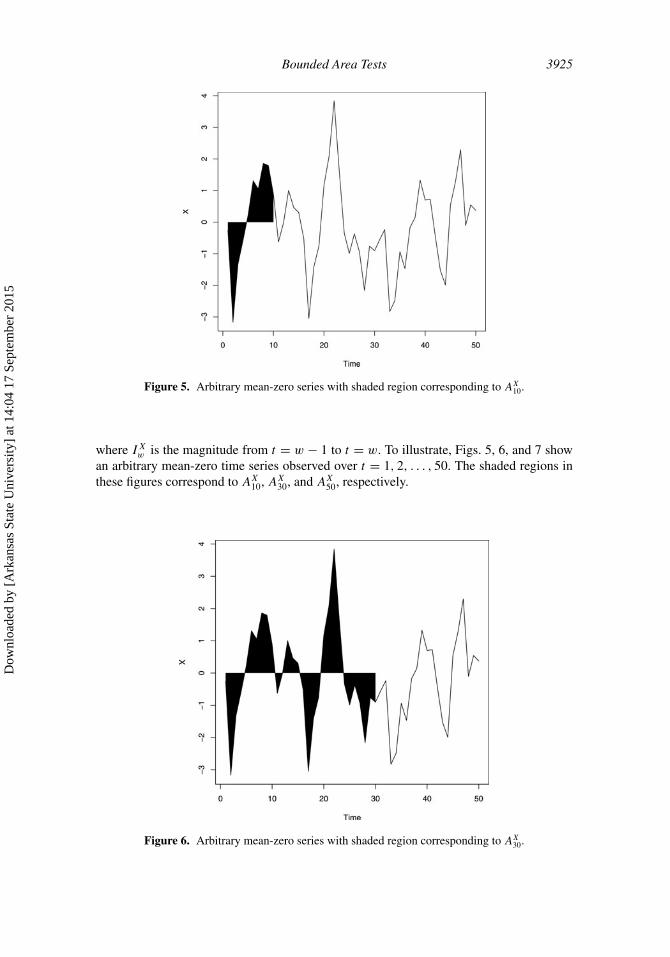
Figure 5. Arbitrary mean-zero series with shaded region corresponding to AX10.

where IXw is the magnitude from t = w − 1 to t = w. To illustrate, Figs. 5, 6, and 7 showan arbitrary mean-zero time series observed over t = 1, 2, . . . , 50. The shaded regions inthese figures correspond to AX10, AX30, and AX50, respectively.

Figure 6. Arbitrary mean-zero series with shaded region corresponding to AX30.

Dow

nloa

ded

by [

Ark

ansa

s St

ate

Uni

vers

ity]

at 1

4:04

17

Sept

embe

r 20

15

3926 Tunno

Figure 7. Arbitrary mean-zero series with shaded region corresponding to AX50.

Now assume that {Xt } follows (1.1). Since {Xt } is a stationary process (in the widesense), so is {IXt }. Thus, we have

Var(AXn

) = Var

(n∑t=2

IXt

)= (n− 1)γIX (0) + 2

n−2∑h=1

(n− 1 − h)γIX (h),

where γIX (h) = Cov(IXt , IXt+h). If {Yt } also follows (1.1), then AYn and its associated func-

tionals are defined analogously.If {Xt } and {Yt } are independent of one another, then given samples X1, X2, . . . , Xn

and Y1, Y2, . . . , Yn, a normalized test statistic for (1.2) is equal to

T = AXn − AYn − E(AXn − AYn

)√Var

(AXn − AYn

) = AXn − AYn − (E(AXn

) − E(AYn

))√Var

(AXn

) + Var(AYn

) .

Under the assumption that the null hypothesis in (1.2) implies E(AXn ) = E(AYn ), we thenhave

TH0= AXn − AYn√

Var(AXn

) + Var(AYn

) . (2.4)

Theorem 2.1. Let {Xt } and {Yt } each follow model (1.1) and be independent of one another.Then, under the assumption of the null hypothesis in (1.2), the test statistic in (2.4) converges

in distribution to the standard normal. That is, TD→ N (0, 1) when H0 is true.

Dow

nloa

ded

by [

Ark

ansa

s St

ate

Uni

vers

ity]

at 1

4:04

17

Sept

embe

r 20

15

Bounded Area Tests 3927

Proof. We will use Corollary 1 of Theorem 1 from Wu (2002). We begin with a list of allrelevant objects concerning sample X1, X2, . . . , Xn:

(A) Xn =∞∑i=0

ψiεn−i

(B) Xn,− =∞∑i=n

ψiεn−i

(C) IXn =∫ n

n−1

∣∣∣(Xn −Xn−1)(u− n) +Xn

∣∣∣ du(D) IXn,− =

∫ n

n−1

∣∣∣(Xn,− −Xn−1,−)(u− n) +Xn,−∣∣∣ du

(E) K(Xn−1, Xn) = IXn − E(IXn

)(F) K(Xn−1,− , Xn,−) = IXn,− − E

(IXn,−

)(A) follows from the causality of (1.1), while (B) is a truncated version of (A). Similarly,

(D) and (F ) are truncated versions of (C) and (E), respectively.Now, observe that

E(K(Xn−1,− , Xn,−))2 ≤ E(IXn,−

)2

≤ E

( ∫ n

n−1

∣∣∣(Xn,− −Xn−1,−)(u− n)∣∣∣ du+

∫ n

n−1|Xn,−| du

)2

= E

( ∣∣∣Xn,− −Xn−1,−∣∣∣ ∫ n

n−1(n− u) du+ |Xn,−|

∫ n

n−1du

)2

= E

( |Xn,− −Xn−1,−|2

+ |Xn,−|)2

≤ vE(Xn,−)2

for some constant v > 0 since |Xn,−−Xn−1,−| < ∞. If ||·|| denotes theL2-norm, it followsthat

∞∑n=2

||K(Xn−1,− , Xn,−)||√n

≤ v1/2∞∑n=2

||Xn,−||√n

= v1/2∞∑n=2

√√√√E

( ∞∑i=n

ψiεn−i

)2 /n

≤ v1/2∞∑n=2

√√√√E

( ∞∑i=n

|ψi |√n

)2 /n

= v1/2∞∑n=2

∞∑i=n

|ψi | < ∞,

Dow

nloa

ded

by [

Ark

ansa

s St

ate

Uni

vers

ity]

at 1

4:04

17

Sept

embe

r 20

15

3928 Tunno

since for any causal ARMA process, we have |ψk| ≤ Crk for some C ∈ R+ and r ∈ (0, 1).

Then, by Corollary 1 of Theorem 1 from Wu (2002), we have

LXK = 1√n

n∑t=2

K(Xt−1, Xt ) = AXn − E(AXn

)√n

D→ N(0, σ 2

K

),

where σ 2K = limn→∞ Var(LXK ). An analogous result holds for {Yt }. Thus, we have

LXK − LYK√Var

(LXK − LYK

) H0= AXn − AYn√Var

(AXn

) + Var(AYn

) D→ N (0, 1)

by Slutsky’s theorem and the independence of {Xt } and {Yt }. �Theorem 2.1 gives us a meaningful way to compare the bounded area magnitudes

for two independent series that both follow (1.1). As will be shown in the next section,a significant difference in bounded area magnitudes implies a significant difference inautocovariance structures. Thus, the bounded area test of size α tells us to reject the nullhypothesis in (1.2) if the magnitude of our test statistic in (2.4) exceeds zα/2, where zα/2is the standard normal critical value with area α/2 to its right. That is, we reject H0 if|T | > zα/2.

It should be noted that in practice γIX (h) is unknown, but Var(AXn ) can still be estimatedwith

Var

(n∑t=2

IXt

)= (n− 1)γIX (0) + 2

[ 3√n]∑h=1

(n− 1 − h)γIX (h), (2.5)

where the non negative definite autocovariance estimator

γIX (h) = 1

n− 1

n−h∑t=2

(IXt − I

) (IXt+h − I

)h = 0, 1, 2, . . . , n− 2

is used with

I = 1

n− 1

n∑t=2

IXt = AXn

n− 1.

The sum in (2.5) is truncated at the greatest integer less than or equal to 3√n in order to avoid

any bias associated with large lags (Berkes et al. 2009, discuss this and other truncationschemes). (2.5) is also a consistent estimator and so if it and its {Yt } analog replace Var(AXn )and Var(AYn ) in the denominator of (2.4), Theorem 2.1 still holds.

3. Simulations

3.1. Set-up

This section compares the Type I error and power of the bounded area test, the timedomain test of Lund et al. (2009), and the arc length test of Tunno et al. (2012) for testing(1.2) at level α = 0.05. In all figures, these tests will be abbreviated as AR, TD, and AL,respectively.

Dow

nloa

ded

by [

Ark

ansa

s St

ate

Uni

vers

ity]

at 1

4:04

17

Sept

embe

r 20

15

Bounded Area Tests 3929

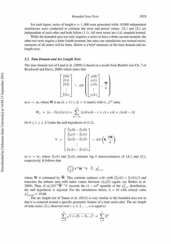
For each figure, series of length n = 1, 000 were generated while 10,000 independentsimulations were conducted to estimate the error and power values. {Xt } and {Yt } areindependent of each other and both follow (1.1). All error terms are i.i.d. standard normal.

While the bounded area test only requires a series to have a finite second moment, theother two tests require a finite fourth moment, but since our simulations use normal errors,moments of all orders will be finite. Below is a brief summary of the time domain and arclength tests.

3.2. Time Domain and Arc Length Tests

The time domain test of Lund et al. (2009) is based on a result from Bartlett (see Ch. 7 ofBrockwell and Davis, 2006) which states that⎡⎢⎢⎢⎢⎢⎣

γ (0)γ (1)γ (2)

...γ (L)

⎤⎥⎥⎥⎥⎥⎦ ∼ AN

⎛⎜⎜⎜⎜⎜⎝

⎡⎢⎢⎢⎢⎢⎣γ (0)γ (1)γ (2)

...γ (L)

⎤⎥⎥⎥⎥⎥⎦ ,Wn

⎞⎟⎟⎟⎟⎟⎠as n → ∞, where W is an (L+ 1) × (L+ 1) matrix with (i, j )th entry

Wij = (η − 3)γ (i)γ (j ) +∞∑

k=−∞[γ (k)γ (k − i + j ) + γ (k + j )γ (k − i)]

for 0 ≤ i, j ≤ L.Under the null hypothesis of (1.2),

V =

⎡⎢⎢⎢⎢⎢⎣γX(0) − γY (0)

γX(1) − γY (1)

γX(2) − γY (2)...

γX(L) − γY (L)

⎤⎥⎥⎥⎥⎥⎦ ∼ AN

(0,

2Wn

)

as n → ∞, where γX(h) and γY (h) estimate lag h autocovariances of {Xt } and {Yt },respectively. It follows that (n

2

)V TW−1V

D→ χ2L+1,

where W is estimated by W. This estimate replaces γ (h) with (γX(h) + γY (h))/2 andtruncates the infinite sum with index values between ±[ 3

√n] (again, see Berkes et al.

2009). Thus, if (n/2)V T W−1V exceeds the (1 − α)th quantile of the χ2L+1 distribution,

the null hypothesis is rejected. For the simulations below, L = 10 with critical valueχ2

11,0.05 = 19.68.The arc length test of Tunno et al. (2012) is very similar to the bounded area test in

that it is centered around a specific geometric feature of a time series plot. The arc lengthof time series {Xt } observed over t = 1, 2, . . . , n is equal to

n∑t=2

√1 + (Xt −Xt−1)2 =

n∑t=2

SXt

Dow

nloa

ded

by [

Ark

ansa

s St

ate

Uni

vers

ity]

at 1

4:04

17

Sept

embe

r 20

15

3930 Tunno

and is simply the sum of the lengths of the n− 1 line segments connecting adjacent pointson the scatter plot (see Figs. 1 and 2). Since {SXt } is stationary, we have

Var

(n∑t=2

SXt

)= (n− 1)γSX (0) + 2

n−2∑h=1

(n− 1 − h)γSX (h),

where γSX (h) = Cov(SXt , SXt+h). All objects are defined analogously for process {Yt }.

If the arc lengths of {Xt } and {Yt } are significantly different, then their autocovariancestructures tend to be as well. The comparison process is made rigorous by utilizing thenormalized test statistic

U =(∑n

t=2 SXt − ∑n

t=2 SYt

) − (n− 1)(E(SXt

) − E(SYt

))√Var

(∑nt=2 S

Xt − ∑n

t=2 SYt

) .

Under the assumption that the null hypothesis in (1.2) implies E(SXt ) = E(SYt ), and that{Xt } and {Yt } are independent of one another, we then have

UH0=

∑nt=2 S

Xt − ∑n

t=2 SYt√

Var(∑n

t=2 SXt

) + Var(∑n

t=2 SYt

) D→ N (0, 1).

Thus, the arc length test of size α rejects the null hypothesis of (1.2) if |U | > zα/2,where zα/2 is the standard normal critical value with area α/2 to its right. Consistentestimators of the variances can be used as surrogates without affecting the test.

3.3. Simulations

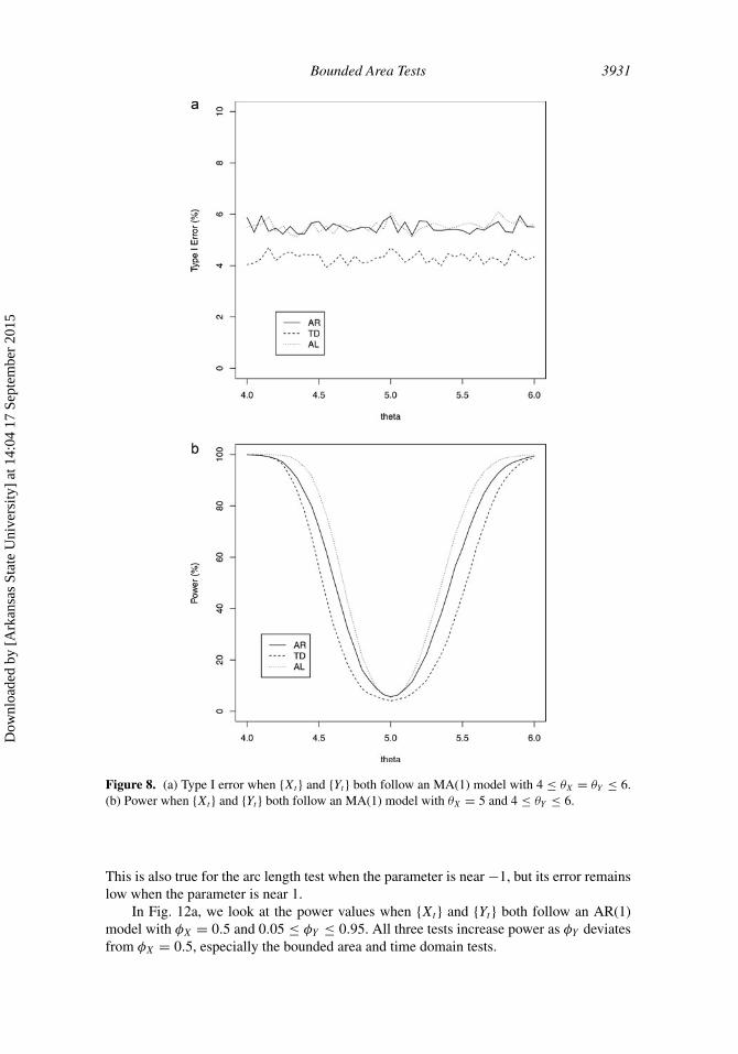
In Fig. 8a, we look at the Type I error values when {Xt } and {Yt } both follow an MA(1)model with 4 ≤ θX = θY ≤ 6. All three tests have a low overall error, especially the timedomain test. In Fig. 8b, we look at the power values when both processes follow an MA(1)model with θX = 5 and 4 ≤ θY ≤ 6. All three tests increase power as the magnitude of θYdeviates from θX = 5.

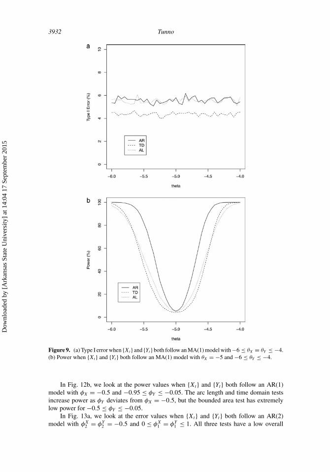
In Fig. 9a, we look at the error values when {Xt } and {Yt } both follow an MA(1) modelwith −6 ≤ θX = θY ≤ −4. All three tests have a low overall error, especially the timedomain test. In Fig. 9b, we look at the power values when both processes follow an MA(1)model with θX = −5 and −6 ≤ θY ≤ −4. All three tests increase power as θY deviatesfrom θX = −5, especially the bounded area test.

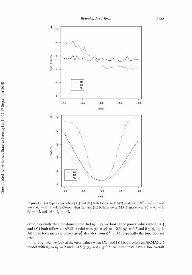
In Fig. 10a, we look at the error values when {Xt } and {Yt } both follow an MA(2)model with θX2 = θY2 = 5 and −6 ≤ θX1 = θY1 ≤ −4. Arc length and bounded area have alow error, but the time domain test has a slightly lower error error for parameter valuesclose to −4 and a slightly higher error for parameter values close to −6. In Fig. 10b, welook at the power values when both processes follow an MA(2) model with θX2 = θY2 = 5,θX1 = −5, and −6 ≤ θY1 ≤ −4. All three tests increase power as θY1 deviates from θX1 = −5,especially the time domain test, although its power may be slightly inflated for parametervalues close to −6.

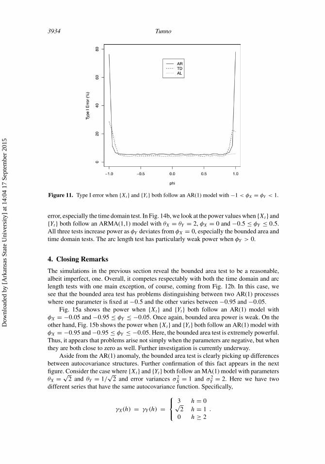
In Fig. 11, we look at the error values when {Xt } and {Yt } both follow an AR(1)model with −1 < φX = φY < 1. All three tests have a low overall error, especially the timedomain test. When the parameter has magnitude near 1 (which is where stationarity breaksdown), the error of the bounded area and time domain tests blow up, especially the former.

Dow

nloa

ded

by [

Ark

ansa

s St

ate

Uni

vers

ity]

at 1

4:04

17

Sept

embe

r 20

15

Bounded Area Tests 3931

Figure 8. (a) Type I error when {Xt } and {Yt } both follow an MA(1) model with 4 ≤ θX = θY ≤ 6.(b) Power when {Xt } and {Yt } both follow an MA(1) model with θX = 5 and 4 ≤ θY ≤ 6.

This is also true for the arc length test when the parameter is near −1, but its error remainslow when the parameter is near 1.

In Fig. 12a, we look at the power values when {Xt } and {Yt } both follow an AR(1)model with φX = 0.5 and 0.05 ≤ φY ≤ 0.95. All three tests increase power as φY deviatesfrom φX = 0.5, especially the bounded area and time domain tests.

Dow

nloa

ded

by [

Ark

ansa

s St

ate

Uni

vers

ity]

at 1

4:04

17

Sept

embe

r 20

15

3932 Tunno

Figure 9. (a) Type I error when {Xt } and {Yt } both follow an MA(1) model with −6 ≤ θX = θY ≤ −4.(b) Power when {Xt } and {Yt } both follow an MA(1) model with θX = −5 and −6 ≤ θY ≤ −4.

In Fig. 12b, we look at the power values when {Xt } and {Yt } both follow an AR(1)model with φX = −0.5 and −0.95 ≤ φY ≤ −0.05. The arc length and time domain testsincrease power as φY deviates from φX = −0.5, but the bounded area test has extremelylow power for −0.5 ≤ φY ≤ −0.05.

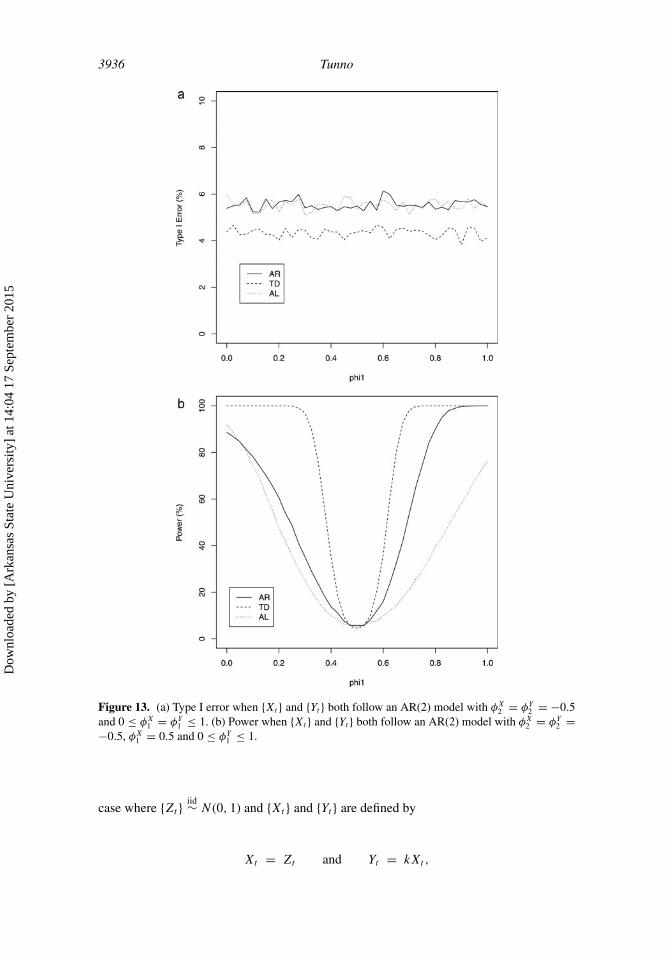
In Fig. 13a, we look at the error values when {Xt } and {Yt } both follow an AR(2)model with φX2 = φY2 = −0.5 and 0 ≤ φX1 = φY1 ≤ 1. All three tests have a low overall

Dow

nloa

ded

by [

Ark

ansa

s St

ate

Uni

vers

ity]

at 1

4:04

17

Sept

embe

r 20

15

Bounded Area Tests 3933

Figure 10. (a) Type I error when {Xt } and {Yt } both follow an MA(2) model with θX2 = θY2 = 5 and−6 ≤ θX1 = θY1 ≤ −4. (b) Power when {Xt } and {Yt } both follow an MA(2) model with θX2 = θY2 = 5,θX1 = −5, and −6 ≤ θY1 ≤ −4.

error, especially the time domain test. In Fig. 13b, we look at the power values when {Xt }and {Yt } both follow an AR(2) model with φX2 = φY2 = −0.5, φX1 = 0.5 and 0 ≤ φY1 ≤ 1.All three tests increase power as φY1 deviates from φX1 = 0.5, especially the time domaintest.

In Fig. 14a, we look at the error values when {Xt } and {Yt } both follow an ARMA(1,1)model with θX = θY = 2 and −0.5 ≤ φX = φY ≤ 0.5. All three tests have a low overall

Dow

nloa

ded

by [

Ark

ansa

s St

ate

Uni

vers

ity]

at 1

4:04

17

Sept

embe

r 20

15

3934 Tunno

Figure 11. Type I error when {Xt } and {Yt } both follow an AR(1) model with −1 < φX = φY < 1.

error, especially the time domain test. In Fig. 14b, we look at the power values when {Xt } and{Yt } both follow an ARMA(1,1) model with θX = θY = 2, φX = 0 and −0.5 ≤ φY ≤ 0.5.All three tests increase power as φY deviates from φX = 0, especially the bounded area andtime domain tests. The arc length test has particularly weak power when φY > 0.

4. Closing Remarks

The simulations in the previous section reveal the bounded area test to be a reasonable,albeit imperfect, one. Overall, it competes respectably with both the time domain and arclength tests with one main exception, of course, coming from Fig. 12b. In this case, wesee that the bounded area test has problems distinguishing between two AR(1) processeswhere one parameter is fixed at −0.5 and the other varies between −0.95 and −0.05.

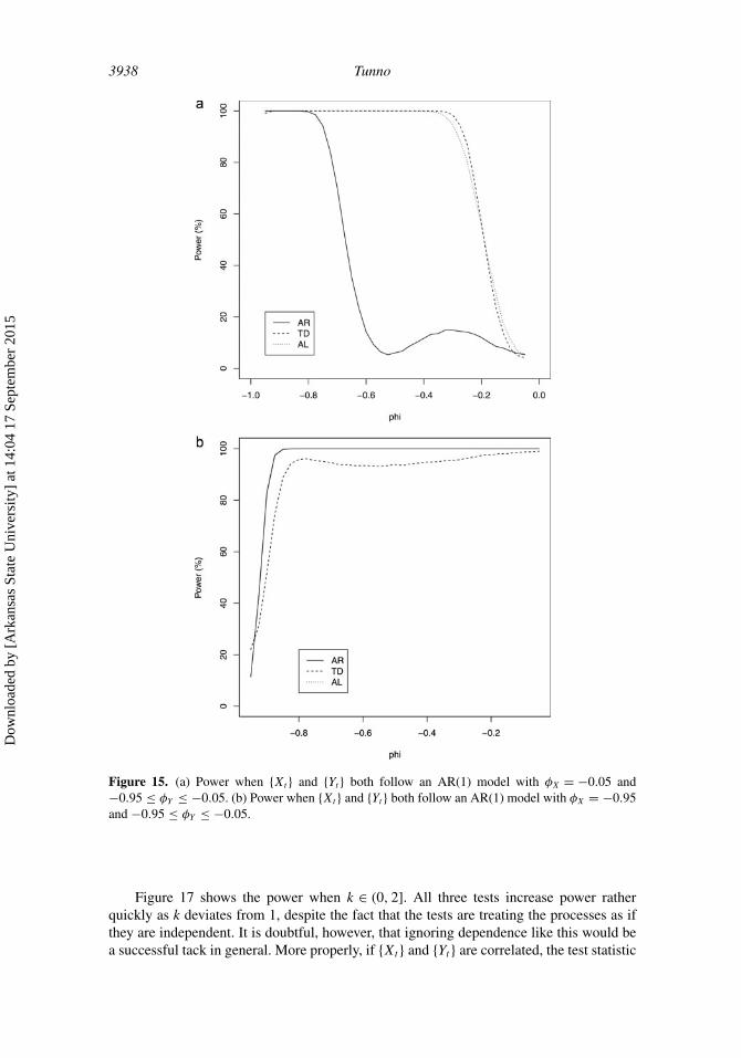
Fig. 15a shows the power when {Xt } and {Yt } both follow an AR(1) model withφX = −0.05 and −0.95 ≤ φY ≤ −0.05. Once again, bounded area power is weak. On theother hand, Fig. 15b shows the power when {Xt } and {Yt } both follow an AR(1) model withφX = −0.95 and −0.95 ≤ φY ≤ −0.05. Here, the bounded area test is extremely powerful.Thus, it appears that problems arise not simply when the parameters are negative, but whenthey are both close to zero as well. Further investigation is currently underway.

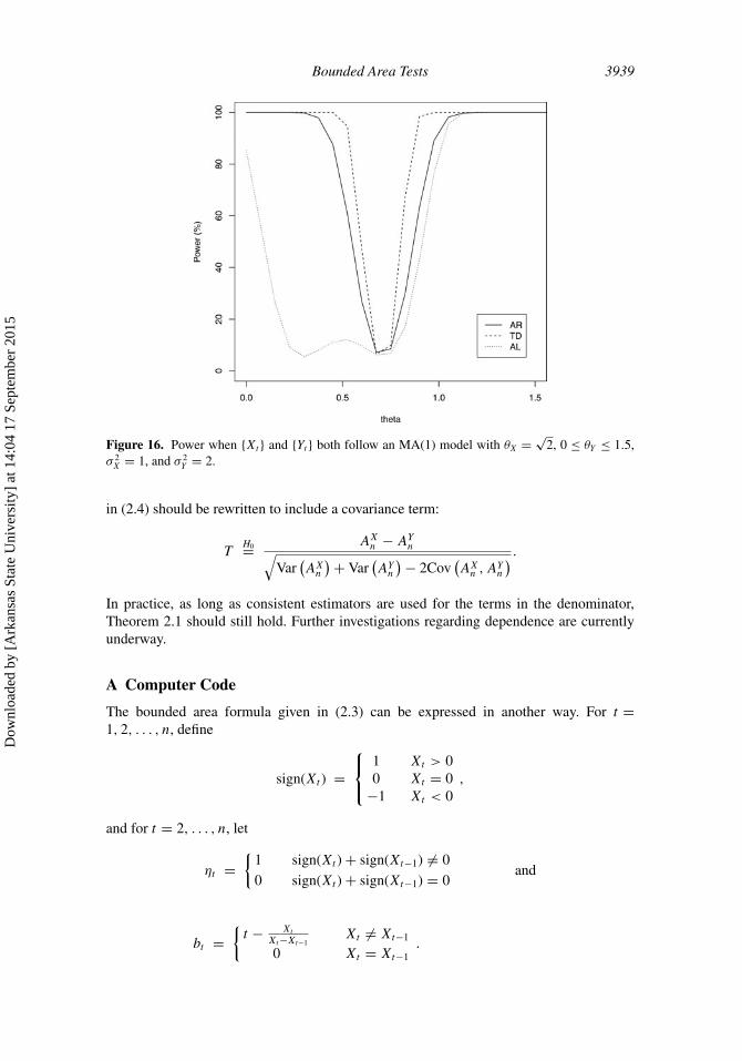
Aside from the AR(1) anomaly, the bounded area test is clearly picking up differencesbetween autocovariance structures. Further confirmation of this fact appears in the nextfigure. Consider the case where {Xt } and {Yt } both follow an MA(1) model with parametersθX = √

2 and θY = 1/√

2 and error variances σ 2X = 1 and σ 2

Y = 2. Here we have twodifferent series that have the same autocovariance function. Specifically,

γX(h) = γY (h) =⎧⎨⎩

3 h = 0√2 h = 1

0 h ≥ 2.

Dow

nloa

ded

by [

Ark

ansa

s St

ate

Uni

vers

ity]

at 1

4:04

17

Sept

embe

r 20

15

Bounded Area Tests 3935

Figure 12. (a) Power when {Xt } and {Yt } both follow an AR(1) model with φX = 0.5 and 0.05 ≤φY ≤ 0.95. (b) Power when {Xt } and {Yt } both follow an AR(1) model with φX = −0.5 and −0.95 ≤φY ≤ −0.05.

Figure 16 shows the power when θY is allowed to range between 0 and 1.5. Both the timedomain and bounded area tests increase power as θY deviates from 1/

√2. The arc length

test becomes erratic when θY < 1/√

2.Future research on this project will include trying to extend the bounded area test to

stationary processes that are not independent from one another. For example, consider the

Dow

nloa

ded

by [

Ark

ansa

s St

ate

Uni

vers

ity]

at 1

4:04

17

Sept

embe

r 20

15

3936 Tunno

Figure 13. (a) Type I error when {Xt } and {Yt } both follow an AR(2) model with φX2 = φY2 = −0.5and 0 ≤ φX1 = φY1 ≤ 1. (b) Power when {Xt } and {Yt } both follow an AR(2) model with φX2 = φY2 =−0.5, φX1 = 0.5 and 0 ≤ φY1 ≤ 1.

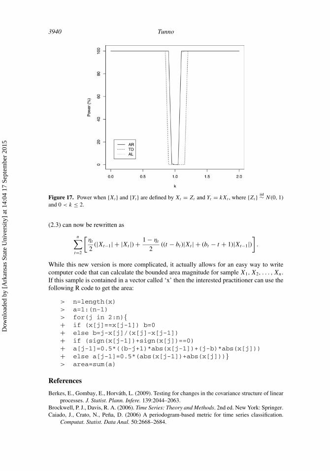
case where {Zt } iid∼ N (0, 1) and {Xt } and {Yt } are defined by

Xt = Zt and Yt = kXt ,

Dow

nloa

ded

by [

Ark

ansa

s St

ate

Uni

vers

ity]

at 1

4:04

17

Sept

embe

r 20

15

Bounded Area Tests 3937

Figure 14. (a) Type I error when {Xt } and {Yt } both follow an ARMA(1,1) model with θX = θY = 2and −0.5 ≤ φX = φY ≤ 0.5. (b) Power when {Xt } and {Yt } both follow an ARMA(1,1) model withθX = θY = 2, φX = 0 and −0.5 ≤ φY ≤ 0.5.

where k is a non zero constant. Then, we have

γY (h) = k2γX(h) and Cov(Xt, Yt ) = k.

Because {Xt } and {Yt } are correlated, they are also dependent.

Dow

nloa

ded

by [

Ark

ansa

s St

ate

Uni

vers

ity]

at 1

4:04

17

Sept

embe

r 20

15

3938 Tunno

Figure 15. (a) Power when {Xt } and {Yt } both follow an AR(1) model with φX = −0.05 and−0.95 ≤ φY ≤ −0.05. (b) Power when {Xt } and {Yt } both follow an AR(1) model with φX = −0.95and −0.95 ≤ φY ≤ −0.05.

Figure 17 shows the power when k ∈ (0, 2]. All three tests increase power ratherquickly as k deviates from 1, despite the fact that the tests are treating the processes as ifthey are independent. It is doubtful, however, that ignoring dependence like this would bea successful tack in general. More properly, if {Xt } and {Yt } are correlated, the test statistic

Dow

nloa

ded

by [

Ark

ansa

s St

ate

Uni

vers

ity]

at 1

4:04

17

Sept

embe

r 20

15

Bounded Area Tests 3939

Figure 16. Power when {Xt } and {Yt } both follow an MA(1) model with θX = √2, 0 ≤ θY ≤ 1.5,

σ 2X = 1, and σ 2

Y = 2.

in (2.4) should be rewritten to include a covariance term:

TH0= AXn − AYn√

Var(AXn

) + Var(AYn

) − 2Cov(AXn ,A

Yn

) .In practice, as long as consistent estimators are used for the terms in the denominator,Theorem 2.1 should still hold. Further investigations regarding dependence are currentlyunderway.

A Computer Code

The bounded area formula given in (2.3) can be expressed in another way. For t =1, 2, . . . , n, define

sign(Xt ) =⎧⎨⎩

1 Xt > 00 Xt = 0

−1 Xt < 0,

and for t = 2, . . . , n, let

ηt ={

1 sign(Xt ) + sign(Xt−1) �= 0

0 sign(Xt ) + sign(Xt−1) = 0and

bt ={t − Xt

Xt−Xt−1Xt �= Xt−1

0 Xt = Xt−1.

Dow

nloa

ded

by [

Ark

ansa

s St

ate

Uni

vers

ity]

at 1

4:04

17

Sept

embe

r 20

15

3940 Tunno

Figure 17. Power when {Xt } and {Yt } are defined by Xt = Zt and Yt = kXt , where {Zt } iid∼ N (0, 1)and 0 < k ≤ 2.

(2.3) can now be rewritten as

n∑t=2

[ηt

2(|Xt−1| + |Xt |) + 1 − ηt

2((t − bt )|Xt | + (bt − t + 1)|Xt−1|)

].

While this new version is more complicated, it actually allows for an easy way to writecomputer code that can calculate the bounded area magnitude for sample X1, X2, . . . , Xn.If this sample is contained in a vector called ‘x’ then the interested practitioner can use thefollowing R code to get the area:

> n=length(x)> a=1:(n-1)> for(j in 2:n){+ if (x[j]==x[j-1]) b=0+ else b=j-x[j]/(x[j]-x[j-1])+ if (sign(x[j-1])+sign(x[j])==0)+ a[j-1]=0.5*((b-j+1)*abs(x[j-1])+(j-b)*abs(x[j]))+ else a[j-1]=0.5*(abs(x[j-1])+abs(x[j]))}> area=sum(a)

References

Berkes, E., Gombay, E., Horvath, L. (2009). Testing for changes in the covariance structure of linearprocesses. J. Statist. Plann. Infere. 139:2044–2063.

Brockwell, P. J., Davis, R. A. (2006). Time Series: Theory and Methods. 2nd ed. New York: Springer.Caiado, J., Crato, N., Pena, D. (2006) A periodogram-based metric for time series classification.

Computat. Statist. Data Anal. 50:2668–2684.

Dow

nloa

ded

by [

Ark

ansa

s St

ate

Uni

vers

ity]

at 1

4:04

17

Sept

embe

r 20

15

Bounded Area Tests 3941

Lund, R., Bassily, H., Vidakovic, B. (2009). Testing equality of stationary autocovariances. J. TimeSer. Anal. 30:332–348.

Tunno, F., Gallagher, C., Lund, R. (2012) Arc length tests for equivalent autocovariances. J. Statist.Computat. Simul. 82:1799–1812.

Wu, W. B. (2002) Central limit theorems for functionals of linear processes and their applications.Statistica Sinica 12:635–649.

Dow

nloa

ded

by [

Ark

ansa

s St

ate

Uni

vers

ity]

at 1

4:04

17

Sept

embe

r 20

15