BEYOND BROWNIANMOTION

Newtonian physics beganwith an attempt to

make precise predictionsabout natural phenomena,predictions that could be ac-curately checked by observa-tion and experiment. Thegoal was to understand na-ture as a deterministic,"clockwork" universe. Theapplication of probability dis-tributions to physics devel-oped much more slowly. Early uses of probability argu-ments focused on distributions with well-defined meansand variances. The prime example was the Gaussian lawof errors, in which the mean traditionally represented themost probable value from a series of repeated measure-ments of a fixed quantity, and the variance was relatedto the uncertainty of those measurements.

But when we come to the Maxwell-Boltzmann distri-bution or the Planck distribution, the whole distributionhas physical meaning. Being away from the mean is nolonger an error, and a large variance is no longer anindicator of poor measurement accuracy. In fact the wholedistribution is the prediction. That was a major concep-tual advance.

In this article we take that idea to its extreme limitand investigate probability distributions, called Levy dis-tributions, with infinite variances, and sometimes eveninfinite means. These distributions are intimately con-nected with fractal random-walk trajectories, called Levyflights, that are composed of self-similar jumps.1 Levyflights are as widely applied in nonlinear, fractal, chaoticand turbulent systems as Brownian motion is in simplersystems.

Brownian motionThe observation of Brownian motion was first reported in1785, by the Dutch physician Jan Ingenhausz. He waslooking at powdered charcoal on an alcohol surface. Butthe phenomenon was later named for Robert Brown, whopublished in 1828 his investigation of the movements offine particles, including pollen, dust and soot, on a watersurface. Albert Einstein eventually explained Brownianmotion in 1905, his annus mirabilis, in terms of random

JOSEPH KLAFTER is a professor in the School of Chemistry atTel Aviv University in Israel. MICHAEL SHLESINGER is chiefscientist for nonlinear science at the Office of Naval Research,in Arlington, Virginia. GERT ZUMOFEN is a lecturer andsenior research scientist at the Laboratory for PhysicalChemistry of the Eidgenossische Technische Hochschule inZurich, Switzerland.

Fractal generalizations of Brownianmotion have proven to be a rich field inprobability theory, statistical physics and

chaotic dynamics.

Joseph Klafter, Michael F. Shlesinger,Gert Zumofen

thermal motions of fluidmolecules striking the micro-scopic particle and causing itto undergo a random walk.

Einstein's famous paperwas entitled "Uber die vonder molekularkinetischenTheorie der Warme gefor-derte Bewegung von inruhenden Flussigkeiten sus-pendierten Teilchen," that isto say, "On the motion, re-

quired by the molecular-kinetic theory of heat, of particlessuspended in fluids at rest." Einstein was primarilyexploiting molecular motion to derive an equation withwhich one could measure Avogadro's number. Apparentlyhe had never actually seen Brown's original papers, whichwere published in the Philosophical Magazine. "It ispossible," wrote Einstein, "that the motions discussed hereare identical with the so-called Brownian molecular mo-tion. But the references accessible to me on the lattersubject are so imprecise that I could not form an opinionabout that."2 Einstein's prediction for the mean squareddisplacement of the random walk of the Brownian particlewas a linear growth with time multiplied by a factor thatinvolved Avogadro's number. This result was promptlyused by Jean Perrin to measure Avogadro's number andthus bolster the case for the existence of atoms. Thatwork won Perrin the 1926 Nobel Prize in Physics.

Less well known is the fact that Louis Bachelier, astudent of Henri Poincare, developed a theory of Brownianmotion in his 1900 thesis. Because Bachelier's work wasin the context of stock market fluctuations, it did notattract the attention of physicists. He introduced whatis today known as the Chapman—Kolmogorov chain equa-tion. Having derived a diffusion equation for randomprocesses, he pointed out that probability could diffuse inthe same manner as heat. (See PHYSICS TODAY, May 1995,page 55.)

Bachelier's work did not lead to any direct advancesin the physics of Brownian motion. In the economiccontext of his work there was no friction, no place forStokes' law nor any appearance of Avogadro's number. ButEinstein did employ all of these ingredients in his theory.Perhaps that illustrates the difference between a mathe-matical approach and one laden with physical insight.

The mathematics of Brownian motion is actually deepand subtle. Bachelier erred in defining a constant velocityv for a Brownian trajectory by taking the limit x/t forsmall displacement x and time interval t. The properlimit involves forming the diffusion constant D =x2lt asboth x and t go to zero. In other words, because therandom-walk displacement in Brownian motion growsonly as the square root of time, velocity scales like r ' •

• 1996 American Institute of Physics, S-0031-9228-96024)30-3 FEBRUARY 1996 PHYSICS TODAY 33

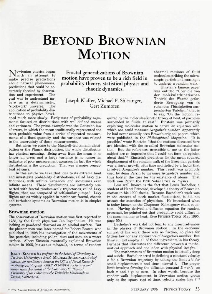
LEVY FLIGHT RANDOM WALK of 1000 steps in twodimensions. For clarity, a dot is shown directly below eachturning point. Limited resolution of this plot makes itdifficult to discern indivdual turning points. They tend tocluster in self-similar patterns characteristic of fractals.Occasional long flight segments initiate new clusters. Thelonger the step, the less likely is its occurence. But Levyflights have no charactensic length. (See the box on page 35.)FIGURE 1

and therefore is not defined in the small-? limit.A Brownian trajectory does not possess a well-defined

derivative at any point. Norbert Wiener developed amathematical measure theory to handle this complication.He proved that the Brownian trajectory is continuous, butof infinite length between any two points. The Browniantrajectory wiggles so much that it is actually two-dimen-sional. Therefore an area measure is more appropriatethan a length measure. Levy flights have a dimensionsomewhere between zero and two.

Among the methods that have been explored to gobeyond Einstein's Brownian motion is fractal Brownianmotion,1 which incorporates self-similarity and producesa trajectory with a mean squared displacement that growswith time raised to a power between zero and two. It isa continuous process without identifiable jumps, and ithas been used to model phenomena as diverse as pricefluctuations and the water level of the Nile. Two otherventures beyond traditional Brownian motion are fractaldistributions of waiting times between random-walk stepsand random walks on fractal structures such as percola-tion lattices. These two examples lead to slower-than-lin-ear growth of the mean squared displacement with time.But in this article we focus on random walk processesthat produce faster-than-linear growth of the mean

squared displacement.Another approach to generalizing Brownian motion is

to view it as a special member of the class of Levy-flightrandom walks. Here we explore applications of Levyflights in physics.3 The interest in this area has grownwith the advent of personal computers and the realizationthat Levy flights can be created and analyzed experimen-tally. The concept of Levy flight can usefully be appliedto a wide range of physics issues, including chaotic phasediffusion in Josephson junctions,4 turbulent diffusion,56

micelle dynamics,7 vortex dynamics,8 anomalous diffusionin rotating flows,9 molecular spectral fluctuations,10 tra-jectories in nonlinear Hamiltonian systems,11"17 moleculardiffusion at liquid-solid interfaces,18, transport in turbu-lent plasma,19 sharpening of blurred images20 and negativeHall resistance in anti-dot lattices.21 In these complexsystems, Levy flights seem to be as prevalent as diffusionis in simpler systems.

Levy flightsThe basic idea of Brownian motion is that of a randomwalk, and the basic result is a Gaussian probabilitydistribution for the position of the random walker after atime t, with the variance (square of the standard deviation)proportional to t. Consider an ./V-step random walk in one

ROTATING-ANNULUS APPARATUS withwhich Harry Swinney's group at theUniversity of Texas investigate Levy

flights and anomalous transport inliquids. The flow is established by

pumping liquid into the rotatingannulus through holes in its bottom.

Showing off the equipment are(clockwise) graduate student Eric Weeks

and postdoc Jeff Urbach. FIGURE 2

34 FEBRUARY 1996 PHYSICS TODAY

400 800TIME (seconds)

1200

O B S E R V I N G FLUID FLOW with tracer

particles in the rotating-annulusapparatus shown in figure 2 revealsa: a state of six stable vortices thatfrequently trap the particle as it circlesaround the annulus. b: In anotherobserved flow state, the particle spendsless time trapped in vortices, c: Plottingazimuthal displacement of severalparticle trajectories against time showsthat the b trajectory (purple), exhibitinglong flights between vortex captures,gets around the annulus much fasterthan the a trajectory (red). (Courtesy ofH. Swinney.) FIGURE 3

dimension, with each step of random length x governedby the same probability distribution p(x), with zero mean.The French mathematician Paul Levy (1886-1971) posedthe question: When does the probability PN(X) for thesum of N steps X = Xx + X2 + . . . + XN have the same dis-tribution p{x) (up to a scale factor) as the individual steps?This is basically the question of fractals, of when does thewhole look like its parts. The standard answer is thatp(x) should be a Gaussian, because a sum of N Gaussiansis again a Gaussian, but with N times the variance of theoriginal. But Levy proved that there exist other solutionsto his question. All the other solutions, however, involverandom variables with infinite variances.

Augustine Cauchy, in 1853, was the first to realizethat other solutions to the Af-step addition of randomvariables existed. He found the form for the probabilitywhen it is transformed from real x space to Fourier kspace:

pN(k) = exp(-AHk I*3) (1)

Cauchy's famous example is the case /3 = 1, which, whentransformed back into x space, has the form

(2)

This is now known as the Cauchy distribution. It showsexplicitly the connection between a one-step and an iV-stepdistribution. Exhibiting this scaling is more importantthan trying to describe the Cauchy distribution in termsof some pseudo-variance, as if it were a Gaussian.

Levy showed that (3 in equation 1 must lie between 0and 2 if p(x) is to be nonnegative for all x, which is requiredfor a probability. Nowadays the probabilities represented inequation 1 are named after Levy. When the absolute valueof x is large, p(x) is approximately Ixl ~1~'3, which impliesthat the second moment of p(x) is infinite when /3 is lessthan 2. This means that there is no characteristic size forthe random walk jumps, except in the Gaussian case of/3 = 2. It is just this absence of a characteristic scale thatmakes Levy random walks (flights) scale-invariant fractals.The box at right makes this more evident with an illustrativeone-dimensional Levy-flight probability function, and figure

A simple Levy-flight random walkonsider a one-dimensional random walk designed to illus-trate the self similarity of Levy flights. Start with the

discrete jump-probability distribution

LA

where b > A > 1 are parameters that characterize the distribu-tion, and 8(x, y) is the Kronecker delta, which equals 1 whenx = y and otherwise vanishes.

This distribution function allows jumps of length 1, b, b2,b3 . . . . But note that whenever the length of the jump increasesby an order of magnitude (in base b), its probability of occurringdecreases by an order of magnitude (in base A). Typically onegets a cluster of A jumps roughly of length 1 before there is ajump of length b. About A such clusters separated by lengthsof order b are formed before one sees a jump of order bl. Andso it goes on, forming a hierarchy of clusters within clusters.

Figure 1 shows a two-dimensional example of this kind ofrandom walk.

The Fourier transform of p(x) is

A-l ~p{k)=—-JjK-icos{b'k)

2.A7=0

which is the famous self-similar Weierstrass function. So wecould call this the Weierstrass random walk. The self-similar-ity of the Weierstrass curve appears explicitly through theequation

1 A - lp(k) = jf(bk) + ^y—cos (k)

which has a small-& solution

with /3 = log (A)/log (b). That is the form of the Levy prob-ability in equation 1 of the main text.

FEBRUARY 1996 PHYSICS TODAY 35

O.JO

0.05

X 0.00 -

0.35 0.40

0.010

0.005

X 0.000

-0.005

-0.010

, b

•

-

1

B

\

t f e •

•

, •

0.275 0.280 0.285 0.290 0.295 0.300

0.003

0.002 -

0.001 •

0.000

FRACTAL COMPLEXITY OF THE CANTORMSLAND STRUCTUREaround a period-3 orbit emerges with successive magnificationsof a plot of the standard map (equation 5) with K = 1.1. a:An orbit with a 3-step period emerges when periodicboundary conditions are imposed in the x direction. Pointsnear this orbit stick close by for some time before comingunder the influence of substructure, b: A tenfoldmagnification of the red island loop in 4a reveals 7 subislands.c: Further expanding the rightmost loop in 4b reveals 10sub-subislands. FlGURJE 4

0.295 0.296 0.297

1 is a plot of 1000 steps of a similar Levy flight in twodimensions.

Despite the beauty of Levy flights, the subject hasbeen largely ignored in the physics literature, mostlybecause the distributions have infinite moments. The firstpoint we wish to make is that one should focus on thescaling properties of Levy flights rather than on theinfinite moments. The divergence of the moments can betamed by associating a velocity with each flight segment.One then asks how far a Levy walk has wandered fromits starting point in time t, rather than what is the meansquared length of a completed jump. The answer to thefirst question will be a well-behaved time-dependent mo-ment of the probability distribution, while the answer tothe second is infinity. Specifically, a Levy random walkermoving with a velocity v, but with an infinite meandisplacement per jump, can have a mean squared dis-placement from the origin that varies as v2 t2. (See thebox on page 37.) Even faster motion is possible if thewalker accelerates, as we shall see when we come to thephenomenon of turbulent diffusion.

Levy walks in turbulenceTo employ Levy flight for trajectories, one introducesvelocity through a coupled spatial-temporal probabilitydensity ty(r, t) for a random walker to undergo a displace-ment r in a time t. We write

ty(r, t) = xp(t I r) p(r) (3)

The factor p(r) is just the probability function, discussedabove, for a single jump. The \f/{t I r) factor is the prob-ability density that the jump takes a time t, given thatits length is r. Let us, for simplicity, make tf/(t I r) theDirac delta function S(t - \r\/v{r)), which ensures thatr = vt. Such random walks, with explicit velocities, visitall points of the jump on the path between 0 and r. Theyare called Levy walks as distinguished from Levy flights,which visit only the two endpoints of a jump.

The velocity v need not be a constant; it can dependon the size of the jump. A most interesting case isturbulent diffusion. In 1926 Lewis Fry Richardson pub-lished his discovery that the mean square of the separationr between two particles in a turbulent flow grows like t3.Dimensional analysis of Brownian motion tells us that<r2(t)>=Dt. This means that the diffusion constant Dcan be endowed with a specific space or time dependence—

36 FEBRUARY 1996 PHYSICS TODAY

0.39

0.34

0.29

0.24

DISTRIBUTION OF TIME it takes astandard-map trajectory (with K - 1.03)to leave the Cantori structure around apenod-5 orbit, plotted as a function ofthe trajectory's initial (x, 0) position.The time distribution exhibits acomplex fractal hierarchy of stickingregions. The black areas mark islandsof stability inside the period-5 orbit,from which a trajectory will neverleave. FIGURE 5

-0.10 0.19

for example, D[r) ~ r1' or D(t) = t2—to produce turbulentdiffusion.

Richardson chose the D(r) = r1'5 route. Note that adiffusion constant has dimensions of [rv]. ThereforeRichardson's 4/3 power law dimensionally implies thatv2(r) scales like r"'\ Then the Fourier transform, v2(k),must scale like k~^3.

This last result, first stated in 1941, is Kolmogorov'swell-known inertial-range turbulence spectrum. Althoughit looks as if Richardson could have predicted the Kolmo-gorov spectrum, the two scaling laws do not necessarilyimply each other. Only if the Kolmogorov scaling(v(r) ~ rV3) is combined with Levy flights (p(r) = r"1"'3), sothat the mean absolute value of r is infinite, does onerecover Richardson's result: <r2(t)> = t3. Up(r) decays fastenough so that all of its moments are finite, then onerecovers the standard Brownian law, even with Kolmo-gorov scaling. The main point here is that the Levy walkwith Kolmogorov scaling describes aspects of turbulentdiffusion. The box on this page shows an example of thepossible scaling laws for the constant-velocity Levy ran-dom walks found in dynamical systems.

An important feature of the Levy-walk approach toturbulent diffusion is that it provides a method for simu-lating trajectories of turbulent particles. Fernand Hayot6

has used this procedure to describe turbulent flow in pipesby means of Levy-walk trajectories with Kolmogorov ve-locity scaling in a lattice gas simulation.

Two-dimensional fluid flowIn two-dimensional computer simulations of fluid flow,James Viecelli8 has found Levy walks and enhanced dif-fusion with mean squared displacement scaling like Vwith y = 1.67forpointvorticesallspinninginthe samesense at high temperatures. At low temperatures thevortices form a rotating triangular lattice. As the tem-perature is raised, the motion of the vortices eventuallybecomes turbulent. The vortices cluster and rotate arounda common center, but now with Levy-walk paths. If bothclockwise and counterclockwise vortices are present, thescaling exponent y becomes 2.6. Oppositely spinningvortices pair and the pairs move in straight-line Levywalks, changing direction when they collide with otherpairs.

These results suggest that two-dimensional rotating

flows are fertile territory for seeking anomalous diffusion.They might serve to approximate large-scale global atmos-pheric and oceanic flows. We predict that Levy walks willbecome increasingly important for understanding globalenvironmental questions of transport and mixing in theatmosphere and the oceans.

Harry Swinney and coworkers at the University ofTexas have been investigating quasi-two-dimensional fluidflow in a rotating laboratory vessel.9 (See figure 2.) In

Mean squared displacementhe mean squared displacement in simple Brownian mo-tion in one dimension has a linear dependence on time

= 2Dt

where D is the diffusion constant and <x2(t)> is the secondmoment of the Gaussian distribution that governs the prob-ability of being at site x at time t. The Gaussian is the hallmarkof Brownian motion. In the case of Levy flights, by contrast,the mean squared displacement diverges. Therefore we con-sider the more complicated random walk described by theprobability distribution of equation 3, which accounts forthe velocity of the Levy walk. For the Kolmogorov turbu-lence case, the velocity depended on the jump size. But herewe consider the simpler constant-velocity case with

being the probability density for time spent in a flight seg-ment. For various values of /8, that leads to the followingdifferent time dependences of the mean square displacement:

t2 for 0 < /3 < 1

<r(t )> =

tV\nt{orp=l

f In t for p = 2

t for 0 > 2

The enhanced diffusion observed in various dynamical sys-tems, such as the standard map (equation 5 in the main text),corresponds to the case 1 < (3 < 2. Similar results, with timedependences ranging from t3 down to r, are found in turbulentdiffusion.

FEBRUARY 1996 PHYSICS TODAY 37

LEVY FLIGHT BEHAVIOR is seen in the trajectory of acomputer-generated Zaslavsky map with fourfold symmetry.13

The random walk starts near the origin and the color ischanged every 1000 steps. FIGURE 6

their experiment, a fluid-filled annulus rotates as a rigidbody. The flow is established by pumping fluid throughholes in the bottom of the annulus. In this nearly two-dimensional flow, neutrally buoyant tracer particles canbe carried along in Levy walks even though the velocityfield is laminar. In fact, Swinney and company were ableto make direct measurements of Levy walks and enhanceddiffusion in this experimental system. (See figure 3.) Aninstability of the axisymmetrically pumped fluid led to astable chain of six vortices, as shown in figure 3a. Tracerparticles were followed to produce probability distributionsfor the distance and time a particle can travel before itgets trapped in a vortex

We use n, the number of vortices passed by a tracerparticle, as a convenient measure of the travel distancer. When a particle leaves a vortex and then passes nvortices in a counterclockwise (or clockwise) fashion beforeit is trapped again, we count that as a random walkerjumping n units to the right (or left) at a constant velocity.In Levy-walk notation, taking ^wajk(t I n) = 8{t - \n\), theUniversity of Texas experimenters found

IH 23= \n\-1~li (4)

and they found that the mean time the particle spendstrapped in a vortex is finite. Under these conditions Levy-walk theory implies that the variance <r2(t)> - <r{t)>2

should scale like t3'13. (See the box on page 37.) Thatturns out to be quite consistent with the experimentaldata, and it gives us a beautiful example of enhanceddiffusion.

Levy walks in nonlinear dynamics: MapsThe Levy-walk case of dynamic scale-invariant circularmotion with constant speed was introduced in 1985 byTheo Geisel and coworkers at the University of Regens-

burg, in Germany^ Their investigations involved thestudy of chaotic phase diffusion in a Josephson junctionby means of a dynamical map, that is to say, a simplerule for generating the nth discrete value of a dynamicalvariable from its predecessor. With a constant voltageacross the junction, the phase rotates at a fixed rate, butit can change direction intermittently. N complete clock-wise voltage-phase rotations correspond to a random walkwith a jump of N units to the right. Analysis of experi-mental data led Geisel and his colleagues to a considera-tion of the nonlinear map .vM = (1 + e)xt + ax\ - 1, with Esmall. Averaging over initial conditions, they found that

t2 forz>2P for 3/2 < z < 2t In t for z = 3/2t for 1 < z < 3/o

where y = 3 - ( z - I)"1. This scaling behavior of the meansquare displacement corresponds to constant-velocity Levywalk with a flight-time distribution between reversalsgiven by i/-(/) = i"1"0, where /3 = 1/(2-1).

In the above example, one can go directly from z, theexponent of the map, to the temporal exponent(3 = 1/(1 -2) for the mean-square displacement. In mostnonlinear dynamical systems, however, the connectionbetween the equations and the kinetics is not obvious orsimple. For example, the so-called standard map:

*n+i = xn + K s\n.2irtin) (5)

has no explicit exponent in sight. But when one plots theprogression of points x, 6, noninteger exponents aboundin the description of the orbit kinetics, hinting at complexdynamics.

Plotting successive (x versus 6) points, at first onemight see simple, nearly closed circular orbits, eventuallygiving way to thoroughly chaotic wandering. But beforechaos sets in one can see orbits that exhibit hierarchicalperiodicities characteristic of the laminar segments of Levywalks. The structures that emerge depend sensitively onthe parameter K. With K= 1.1, for example, we see (infigure 4a) a period-3 orbit. The heirarchical, fractal nature

38 FEBRUARY 1996 PHYSICS TODAY

1500

1000 -

1500

THROUGH AN EGG-CRATE potential in the x, y plane, acomputer-generated lO -̂step random walk exhibits Levy flight.The second moment of the step-length distribution is infinite.Between long flights, the trajectory gets trapped intermittentlyin individual potential wells. FIGURE 7

of its three loops (called Cantori islands, because theyform something like a Cantor set of tori) is revealed inthe successively magnified plots of figures 4b and 4c. Thisfractal regime, describing complex kinetics with Levystatistics, has been dubbed "strange kinetics."16

Figure 5 shows the distribution of the time a stand-ard-map x-versus-^ trajectory spends around a period-5Cantori orbit that emerges when K= 1.03. The timedistribution exhibits a complex fractal hierarchy of stick-ing regions in the phase space. The probability densitiesfor spending time in laminar states near period-3 andperiod-5 orbits have, respectively, the Levy scaling behav-iors r 2 2 and r2 8 .

Another example of Levy walks in dynamical systemsis provided by the orbits in a map devised by GeorgeZaslavsky of the Courant Institute.1213 These walks forman intricate fractal web throughout a two-dimensionalphase space. The Zaslavsky map has only simple trigo-nometric nonlinearities but, like the standard map, itrequires noninteger exponents for the characterization ofits trajectories. Figure 6 shows a Levy-like trajectory ina 4-fold symmetric Zaslavsky map.

PotentialsOne might expect that motion in a simple periodic potentialshould look simple. But closer inspection of the phase-space structure of trajectories in a simple two-dimensionalegg-crate potential reveals a behavior as rich as what weget from the standard and Zaslavsky maps11"1315. It turnsout that Levy walks emerge quite naturally in such po-tentials, and one finds enhanced diffusion. See figure 7.Although the trajectories possess long walks with Levyscaling in the x and y directions of the egg-crate array,the motion is complicated by intermittent trapping in thepotential wells-. This trapping is related to the observedvortex sticking of tracer particles in the Swinney group'sexperiment. In neither case is the distribution of such"localizing" events broad enough to affect the predictedenhanced-diffusion exponent.

Levy walks also appear for time-dependent potentials.Igor Aranson and colleagues at the Institute for AppliedPhysics in Nizhny Novgorod (formerly Gorky) in Russia,investigated a potential that varies sinusoidally in timeand found that it produces Levy walks similar to thoseone gets with static egg-crate potentials. All of these

examples indicate that we are exploring an exciting, wide-open field when we venture beyond the traditional confinesof Brownian motion.

We thank Harry Swinney for providing his experimental resultsand for sharing his insights into Levy walks in fluids. We alsothank George Zaslavsky for illuminating discussions and forsuggesting the Levy walk shown in figure 6.

References1. B. Mandelbrot, The Fractal Geometry of Nature, Freeman, San

Francisco (1982).2. A. Einstein, Annalen der Physik 17, 549 (1905).3. Levy Flights and Related Topics in Physics, M. Shlesinger, G.

Zaslavsky, U. Frisch, Eds., Springer, Berlin (1995).4. T. Geisel, J. Nierwetberg, A. Zacherl, Phys. Rev. Lett. 54, 616

(1985).5. M. Shlesinger, B. West, J. Klafter, Phys. Rev. Lett. 58, 1100

(1987). M. Shlesinger, J. Klafter, Y. M. Wong, J. Stat. Phys.27,499(1982).

6. F. Hayot, Phys. Rev. A. 43, 806 (1991).7. A. Ott, J. Bouchaud, D. Langevin, and W. Urbach, Phys. Rev.

Lett. 65, 2201 (1990). J. Bouchaud, A. Georges, Phys. Reports195, 127(1980).

8. J. Viecelli, Phys. Fluids A 5, 2484 (1993).9. T. Solomon, E. Weeks, H. Swinney, Phys. Rev. Lett. 71, 3975

(1993).10. G. Zumofen, J. Klafter, Chem. Phys. Lett. 219 303 (1994).11. T. Geisel, A. Zacherl, G. Radons. Z. Phys. B. 71, 117 (1988).12. A. Chernikov, B. Petrovichev, A. Rogalsky, R. Sagdeev, G.

Zaslavsky, Phys. Lett. A 144, 127 (1990).13. D. Chaikovsky, G. Zaslavsky, Chaos 1, 463 (1991).14. I. Aranson, M. Rabinovich, L. Tsimring, Phys. Lett. A151, 523

(1990).15. J. Klafter, G. Zumofen, Phys. Rev. E 49, 4873 (1994).16. M. Shlesinger, G. Zaslavsky, J. Klafter, Nature 363,31 (1993).17. R. Ramashanker, D. Berlin, J. Gollub, Phys. Fluids A 2. 1955

(1980).18. O. Baychuk, B. O'Shaughnessy, Phys. Rev. Lett 74, 1795

(1985). S. Stapf, R. Kimmich, R. Seitter, Phys. Rev. Lett. 75,2855(1995).

19. G. Zimbardo, P. Veltrei, G. Basile, S. Principato, Phys. Plasma2, 2653 (1995). R. Balescu, Phys. Rev. E 51, 4807 (1995).

20. A. Carasso, in Mathematical Methods in Medical Imaging II,SPIE vol. 2035 (1993), p. 255.

21. R. Fleischmann, T. Geisel, R. Ketzmerick, Europhys. Lett. 25,219(1994). •

FEBRUARY 1996 PHYSICS TODAY 39