beyond fico: default prediction and optimal lending

Beyond FICO: Default Predictionand Optimal Lending Strategies

in Online P2P InvestingThe Harvard community has made this

article openly available. Please share howthis access benefits you. Your story matters

Citable link http://nrs.harvard.edu/urn-3:HUL.InstRepos:38811439

Terms of Use This article was downloaded from Harvard University’s DASHrepository, and is made available under the terms and conditionsapplicable to Other Posted Material, as set forth at http://nrs.harvard.edu/urn-3:HUL.InstRepos:dash.current.terms-of-use#LAA

http://osc.hul.harvard.edu/dash/open-access-feedback?handle=&title=Beyond%20FICO:%20Default%20Prediction%20and%20Optimal%20Lending%20Strategies%20in%20Online%20P2P%20Investing&community=1/1&collection=1/4927603&owningCollection1/4927603&harvardAuthors=0a4f14d6c9f7113d509024f30dc33263&department

http://nrs.harvard.edu/urn-3:HUL.InstRepos:38811439

http://nrs.harvard.edu/urn-3:HUL.InstRepos:dash.current.terms-of-use#LAA



Acknowledgements

I would first like to thank my adviser Yaron Singer for all of his help through this process. From

iterating through what seemed like a dozen ideas to providing the inspiration for what would

eventually become this thesis to reviewing my analyses and writing, his assistance has been

invaluable. I would also like to thank John Campbell for agreeing to read my paper without

hesitation and helping me work through the theoretical foundations for the economic analysis of

investment strategies that has become the cornerstone of this project. I am especially thankful

for him because without his class Economics 1723, I would have never had the insight to turn

what was initially a project about predicting defaults to a much more interesting project about

investment optimization. Additional thanks go to LendingClub for making their data public and

thereby facilitating such endeavors. I am especially indebted to my friends and family for their

warmth and support.

Special thanks go to late night pizza deliveries from the Dominos Pizza in Harvard Square,

without which this thesis realistically would never have been completed.

2

Contents

1 Introduction 6

2 Preliminaries 9

2.1 LendingClub: A Primer . . . . . . . . . . . . . . . . . . . . . . . . . . . . . . . . 9

2.2 Literature Review . . . . . . . . . . . . . . . . . . . . . . . . . . . . . . . . . . . 12

2.2.1 On Borrowers and Default Risk . . . . . . . . . . . . . . . . . . . . . . . . 13

2.2.2 On Online P2P Investing . . . . . . . . . . . . . . . . . . . . . . . . . . . 14

3 Dataset 18

3.1 Features . . . . . . . . . . . . . . . . . . . . . . . . . . . . . . . . . . . . . . . . . 19

3.2 Variable Sets . . . . . . . . . . . . . . . . . . . . . . . . . . . . . . . . . . . . . . 27

4 Default Prediction 28

4.1 Methods . . . . . . . . . . . . . . . . . . . . . . . . . . . . . . . . . . . . . . . . . 29

4.1.1 Balancing the Dataset . . . . . . . . . . . . . . . . . . . . . . . . . . . . . 30

4.1.2 Ranked Optimal Subset Algorithm . . . . . . . . . . . . . . . . . . . . . . 31

4.2 Overview of Classification Methods . . . . . . . . . . . . . . . . . . . . . . . . . . 32

4.2.1 K-Nearest Neighbors . . . . . . . . . . . . . . . . . . . . . . . . . . . . . . 33

4.2.2 Decision Tree . . . . . . . . . . . . . . . . . . . . . . . . . . . . . . . . . . 34

4.2.3 Linear Regression . . . . . . . . . . . . . . . . . . . . . . . . . . . . . . . . 35

4.2.4 Logistic Regression . . . . . . . . . . . . . . . . . . . . . . . . . . . . . . . 36

4.3 Results . . . . . . . . . . . . . . . . . . . . . . . . . . . . . . . . . . . . . . . . . . 37

4.3.1 Overall Results . . . . . . . . . . . . . . . . . . . . . . . . . . . . . . . . . 37

3

4.3.2 Variable Set Results . . . . . . . . . . . . . . . . . . . . . . . . . . . . . . 39

4.4 Marginal Value of FICO Score . . . . . . . . . . . . . . . . . . . . . . . . . . . . 46

4.5 Default Probability . . . . . . . . . . . . . . . . . . . . . . . . . . . . . . . . . . . 47

5 Investment Strategy Analysis 49

5.1 Methods . . . . . . . . . . . . . . . . . . . . . . . . . . . . . . . . . . . . . . . . . 50

5.1.1 Mean-Variance Analysis of a Loan . . . . . . . . . . . . . . . . . . . . . . 50

5.1.2 Mean-Variance Analysis of a Portfolio of Loans . . . . . . . . . . . . . . . 52

5.2 Calculating the Loan Correlation . . . . . . . . . . . . . . . . . . . . . . . . . . . 54

5.3 Analysis of Grade Allocation . . . . . . . . . . . . . . . . . . . . . . . . . . . . . 56

5.4 Optimal Grade Allocation . . . . . . . . . . . . . . . . . . . . . . . . . . . . . . . 57

5.5 Analysis of Filtering Strategies . . . . . . . . . . . . . . . . . . . . . . . . . . . . 59

5.6 Optimal Filters . . . . . . . . . . . . . . . . . . . . . . . . . . . . . . . . . . . . . 65

5.7 Introduction of Novel Analysis Tool . . . . . . . . . . . . . . . . . . . . . . . . . 67

6 Conclusion 68

Appendices 72

A Additional Information 73

A.1 Application Screenshots . . . . . . . . . . . . . . . . . . . . . . . . . . . . . . . . 73

A.2 LendingClub Screenshots . . . . . . . . . . . . . . . . . . . . . . . . . . . . . . . 74

A.3 Subgrade Statistics and Predictions . . . . . . . . . . . . . . . . . . . . . . . . . . 75

A.4 Visualization of Loans by Geography . . . . . . . . . . . . . . . . . . . . . . . . . 77

A.5 Pseudocode for Ranked Optimal Subset Algorithm . . . . . . . . . . . . . . . . . 78

A.6 Additional Classification Methods . . . . . . . . . . . . . . . . . . . . . . . . . . 79

A.6.1 Perceptron Algorithm . . . . . . . . . . . . . . . . . . . . . . . . . . . . . 79

A.6.2 Support Vector Machine . . . . . . . . . . . . . . . . . . . . . . . . . . . . 80

A.6.3 Boosted Decision Tree . . . . . . . . . . . . . . . . . . . . . . . . . . . . . 81

B Additional Data 82

B.1 Additional Default Prediction Results . . . . . . . . . . . . . . . . . . . . . . . . 82

4

B.2 FICO Comparison Results . . . . . . . . . . . . . . . . . . . . . . . . . . . . . . . 85

B.3 Grade Allocations for Filtering Strategies . . . . . . . . . . . . . . . . . . . . . . 87

Bibliography 89

5

Chapter 1

Introduction

Over the last decade, against the backdrop of the financial recession, a radical new form of

lending known as online P2P (Peer-to-Peer or People-to-People) lending has grown tremendously,

disrupting traditional financial intermediation and changing the landscape of the credit markets.

The fundamental premise behind this new form of lending is that borrowers can apply online

for loans and other individuals can fund these loans and receive interest payments, potentially

making substantial returns. Dominated by U.S. based LendingClub and Prosper and U.K. based

Zopa, these companies have suceeded not only due to their ability to provide credit at lower rates

than borrowers other might receive, but also by introducing a lucrative, alternative asset class

for investors [48]. Indeed, this ability of investors to potentially outperform the market with

these loans has spawned a huge community of investors (see LendAcademy, LendingMemo), as

well as automatic investing services (LendingRobot), a secondary market (Folio) and retirement

accounts on several platforms.

An effect of this is a huge variety of information as to the best strategies to utilize P2P

lending platforms. A cursory glance at these investment communities yields vastly different

optimal strategies, largely based on anecdotal evidence of high returns. Some investors believe

in only investing in low-risk loans while others believe the opposite. Still more believe in investing

in a variety of risk levels, but disagree on the specific allocation. It is in this conflict of opinions

that our motivating problem emerges.

6

Our thesis has two main goals:

1. Using publicly available data from LendingClub to develop a framework for analyzing

lending strategies on Online P2P Marketplaces and, in doing so, develop a set of optimal

investment strategies.

2. Analyze the features that affect default in Online P2P Loans, specifically focusing on

determining predictive value of the FICO Score, which has had its effectiveness questioned

in recent times, and the Lending Club assigned subgrade of the loan [44].

The framework we introduce, based largely on modern portfolio theory and the ideas of ex-

pected value, fundamentally consists of viewing an lending strategy as the purchase of a portfolio

of loans, each of which has a mean and variance [33]. Thus, the default prediction question fol-

lows naturally from that of determining optimal lending strategies, as a determination of the

probability of default is essential to calculating the mean and variance of a loan. To investigate

default, we first use several machine learning methods to classify the loans into ”default” and

”paid off”, in an extension of a fairly common machine learning problem. In our analysis of the

causes of default, we noticed that the subset of features used in classification has a large effect on

the predictive accuracy of a loan classifier. Furthermore, though a few studies have shown which

features in the Lending Club dataset are most predictive of default, hardly any have separated

features into subsets in an attempt to determine the effect of including or excluding a certain

feature from the classifier [44]. We seek to extend these analyses of the LendingClub dataset by

doing just that. By ascertaining and quantifying the effects of each feature on default, we hope

to provide insights into the drivers of default not only in LendingClub but in personal credit

markets more generally. In doing so, we hope to inform both borrowers and investors, for, as

we will discuss throughout this work, default is the single most important determinant of the

success of an investment strategy and minimizing perceived likelihood of default is paramount

to obtaining lower rates for borrowers.

The thesis is structured in the following way. Chapter 2 provides background information

on Lending Club, including previous studies on the subject, to better understand the envi-

ronment in which our analyses take place. In Chapter 3, we provide a brief outline and ex-

ploratory investigation of the LendingClub dataset that we used for our analysis to better

7

understand the features and terminology used throughout the remainder of the work. After

these preliminaries, we dive into the issue of default prediction in Chapter 4, discussing the

various methods and statistical learning techniques used in the analysis as well as their re-

sults. We devote Chapter 5 to the discussion of the two major investment decisions all Lend-

ingClub investors must make: determining the allocation of their portfolio and determining

which (if any) filters to use in the dataset. Finally, we provide concluding remarks in Chap-

ter 6. As we will show, while various methods can approximate optimal strategies, with mil-

lions of allocation-filter combinations, finding optimal points can be quite complex. To aid in

this process, we introduce an online application to simultaneously test allocations and filter-

ing strategies using the framework developed in the rest of the work. This application can be

found at http://kunalmehta-thesis-dev.us-west-2.elasticbeanstalk.com and

screenshots can be seen in Appendix A.1.

8

Chapter 2

Preliminaries

In this section, we seek to ground this thesis in its larger context. Because we focus on Lending-

Club exclusively in the analyses to come, we first provide an extensive overview of the platform

itself, as well as the terminology and mechanisms that the platform uses. In addition, we also

review some of the existing literature on default prediction and investment optimization on

LendingClub and online lending more generally.

2.1 LendingClub: A Primer

LendingClub describes itself in the following way:

”We are the world’s largest online credit marketplace, facilitating personal loans,

business loans, and financing for elective medical procedures. Borrowers access lower

interest rate loans through a fast and easy online or mobile interface. Investors

provide the capital to enable many of the loans in exchange for earning interest [13].”

For our purposes, this description is succinct and quite apt. Indeed, LendingClub can be

summarized as having two main functions: (1) providing borrowers with a way to apply for and

access loans and (2) allowing investors to fund those same loans. We will discuss each of these

functions in depth by way of a look at the life of a loan.

9

Directly from LendingClub’s home page, borrowers can check their rates by entering their

FICO Credit Range, the purpose of their loan and their required amount (up to $25,000) [7].

Following this preliminary questionnaire, they then fill out a simple form with basic personal

information as well as annual income. Once they submit this form, they allow LendingClub to

verify their income and additionally agree to various legally binding documents. LendingClub

will then instantly provide them with an assigned grade (A-G) and subgrade (1-5) and a cor-

responding interest rate and a term length for various loans that they qualify for depending on

their credit characteristics [10]. Loans classified as A1 are considered the safest and have the

lowest corresponding interest rates and those in grade G5 the most risky and therefore require

the highest interest rate. Appendix A.3 provides a detailed breakdown of the grades and cor-

responding interest rates for the loans. Once borrowers choose a loan and term, they fill out

additional employment and bank account information and, a few hours later, after additional

verification, the loan is listed on the LendingClub online marketplace.

For the borrower, paying back the loan is simple. They are given an amortized payment

schedule relating to their loan amount and interest rate and must make the required monthly

payment until the loan matures (either 36 or 60 months). For more information on this process,

please see LendingClub and SocialLendingNetwork [7, 10]. For an example of a loan payment

schedule please see LendingMemo [35].

Investors, upon signing in to LendingClub, see a marketplace of available loans as well as an

interface to view the status of their invested loans (see Appendix A.2 for visualizations of these

interfaces) [13]. Upon deciding on investing in a loan, an investor can fund as little as $25 of the

loan, allowing for significant diversification across loans. Let’s say our investor decides to lend

$25 in the loan from above. Then, over the next few days (LendingClub’s average funding time

is approximately seven days, according to their website), other investors will purchase portions

of the loan until the full amount has been funded [8]. At this point, the borrower receives the

amount of the loan in their bank account and must make required payments each month. They

may additionally prepay the amount of the principal at any time.

Investors face two primary risks to their returns: (1) default risk and (2) prepayment risk.

Default risk naturally refers to the likelihood that a borrower does not pay back the loan, thereby

preventing the investor from earning the agreed-upon return. Traditional financial intermediaries,

10

as well as LendingClub investors, are most concerned with this risk as it poses the highest risk

to their returns, often even causing large losses to the investor. Prepayment risk refers to ther

likelihood that a borrower pays the principal off early, thereby preventing the investor from

earning the entirety of the interest paid over the full term of the loan. While prepayment risk

is difficult to classify, LendingClub provides a number of labels that inform the investor as to

the current default status of the loan. We have summarized these in Table 2.1 and additionally

provided the number of loans in our dataset that fit each label.

Status Description Number

Current The loan is currently being paid off on time. 428,294Fully Paid The loan was fully paid off. 163,412Grace Period Payments are late by 15 days or less on this loan. 5155Late (16-30 days) Payments are late by 16-30 days on this current loan. 1952Late (31-120 days) Payments are late by 31-120 days on this current loan. 9215Defaulted Payments are late by 31-120 days on this loan. 223Charged Off LendingClub believes that there further payments on this loan

are unlikely. Payments are 150 days past due date.35,389

Table 2.1: Loan Status Categories from LendingClub [12]

When a borrower misses a payment, LendingClub enacts a process that attempts to return

the loan to ”Current” status [7]. If after 150 days, the borrower has not restarted payments on

the loan, the loan is ”charged off”, which is essentially default beyond the point of recovery. At

this point, LendingClub believes any attempt to reacquire the value of the loan are fundamentally

futile. Nonetheless, LendingClub outsources collection of charged off loans to a third-party but

admits that any recoveries after the loan is charged off are ”infrequent” [7].

LendingClub profits off this process in several ways. First, investors are charged a 1% service

fee for each purchase. Additionally, LendingClub charges 30% of any collections made after the

loan is classified as late and 30% of attorney fees and costs in the case of litigation [7]. This

fee structure undoubtedly has been successful for the company, leading to a $400 million dollar

revenue in 2015 [22].

We have hitherto discussed the investment and payment process for a single loan. However,

hardly any investors purchase a single loan. In fact, most do not even manually select which

loans to purchase, instead utlizing LendingClub’s propietary ”Automated Investing” tool. Here

investors can use two tools to craft an investment strategy

11

1. Grade Allocation: Investors can select an allocation of grades A-G they would like to

invest their funds in. LendingClub also has some predefined allocations, which we will

discuss in Chapter 5.

2. Filters: Investors can filter based on the features discussed further in Chapter 3 by selecting

a variable and a cutoff amount. For example, investors can choose to invest only in loans

whose borrowers have an income of greater than $50,000 per year. When a filter conflicts

with a grade allocation, the automated investor notifies the borrower and ceases activity.

Investors can also sell loans through LendingClub’s Note Trading Platform (in partnership

with Folio Investing) [11]. Without this platform, however, investors must hold the loans through

maturity. LendingClub claims that 99.9% of investors with more than $2,500 invested in more

than 100 loans see positive returns on their investment, a claim that will be addressed in the next

few chapters [23]. Primarily due to the novelty of online lending, there seems to be a relative

dearth in academic discussion regarding issues of default prediction and investment optimization

in online lending, with much of the work in the field coming from informal sources, mostly

investment forums and the like. We review both types of research in the next section, as both

provide insights into the data.

2.2 Literature Review

We first look at works that provide an overview of the P2P Lending, often comparing it to

traditional intermediaries. Wang, Greiner and Anderson provide perhaps the most complete

overview of the concept of online peer lending, categorizing LendingClub, Prosper and Zopa

into Profit-Seeking Lending Models, one of the four quadrants of a matrix separated by what

they see as the two main factors that differentiate lending models: motive of lending (economic

or philanthropic) and degree of separation (friends or strangers) [48]. Furthermore, they note

that ”the value proposition of P2P lending for borrowers is that they are able to obtain loans

with lower interest rates than bank loan rates...[and the] value proposition for lenders is that

P2P loans offer an alternative investment option [48]”. Berger and Gleisner not only provide an

excellent overview of the history and existing literature on Online P2P Lending, but also discuss

12

the now-discontinued group dynamic on Prosper, in which ”screening of potential borrowers and

monitoring of loan repayment can be delegated to designated group leaders [24]”. They find that

these group leaders serve as financial intermediaries not dissimilar to banks in terms of their

ability to reduce information asymmetries, thereby improving credit conditions [24].

Wang, Chen, Zhu and Song model online P2P Lending as a process, noting interesting dis-

tinctions between the process in P2P lending versus traditional lending [47]. They conclude

that ”P2P lending provides users more privilege in choosing the lending manner and lending

objects...so the information flow...is more frequent and transparent”, but also find that loan

management is subpar in online P2P lending as compared to a traditional bank, mostly due to

its inability to track post-loan information as well [47]. Zeng and Brill both look at the legal

framework for P2P lending with different perspectives. While Zeng takes a global approach, Brill

specifically looks at how the Dodd-Frank act effects the online lending environment [50, 25].

2.2.1 On Borrowers and Default Risk

The most expansive academic literature about peer-to-peer lending focuses on the borrowers, de-

termining different qualities that effect their ability to receive credit. We have already mentioned

how Berger and Glesiner find that group leaders serve as financial intermediaries, improving

credit conditions. Ghasemkhani and Tan look at how reputations affect borrowing ability, using

an unnamed online marketplace that provides borrowers history of loans on the marketplace [31].

Gonzalez and McAleer show that higher amounts and certain purposes slow funding in Prosper

and Zopa and that the number of lenders increases with higher credit ratings and loan sizes,

indicating ”lenders set limits as per rule of thumb in terms of diversification [32]”. Pope and

Sydnor, in an appalling study, find that racial disparities between profile pictures on Prosper

affect interest rates and ability to obtain credit, finding that those with darker skin tend have

higher interest rates and default rates than those with whiter skin, on average [42].

LendingClub, in its current form, is a much simpler platform than many of those studied in

previously mentioned articles. Its data consists of a number of numeric features, excluding most

identifying information of a member. As such, our default prediction methodology focused on

these numeric features, detailed in Chapter 3. However, a few studies have emerged focusing on

13

this very problem, though many are still quite distinct from the default prediction analysis we

conduct in Chapter 4.

A study from the University of Zaragoza analyzes the various features on the data available

publicly on LendingClub using a logistic regression to predict default. The study finds that

the grade assigned by LendingClub is the most predictive, but other factors are also predictive,

especially the debt-to-income ratio [44]. Machine learning blog yhat studies the same dataset

and uses a random forest to predict loan defaults, creating an analysis tool that allows one to

input various parameters to return a probability of default [49]. Cunningham also provides an

interesting history of defaults on Lending Club, showing how the company’s move upward to a

borrower’s average FICO Score of 700 decreased the default rate overall of borrowers [29]. In

determining default, we also want to consider the effects of the LendingClub assigned grade and

the FICO Score on default and thus investment strategy analysis. While the Zaragoza study and

the yhat application provide some insights into these effects, our isolation of the FICO Score

was primarily due to recent research that suggests that the FICO Score as a measure of credit

risk may need to be rethought. In particular, a joint study by Istanbul Sehir University and

Johns Hopkins uses LendingClub data to find that ”the traditional credit scoring methods fall

short in identifying risky borrowers and that social lending has different dynamics compared to

traditional lending [26]”. Additionally, they note that so-called ”social data” is important to

consider.

These studies, for the most part, differ from ours primarily in that they lack an analysis of the

marginal value add in predictive accuracy by various features. As we will discuss in Chapter 4,

our formulation allows us to generally understand the effect of these features on default in a more

nuanced way than the previous analyses, though the models constructed in previous studies are

sometimes more involved than the ones used in our analysis.

2.2.2 On Online P2P Investing

In terms of previous research on investment strategies in LendingClub, specifically analysis of

grade allocations and filters, the academic publications are few and far between. Ethan Namvar

writes an article outlining Online P2P loans as an investment strategy, detailing several online

14

marketplaces, diversification strategies among P2P loans and between P2P loans and asset classes

[40]. He further lists several risks inherent with investing in online loans: regulatory, default,

prepayment and liquidity [40]. However, the article does not supplement its analysis with any

details on investment strategy, rather simply indicates that the investment opportunities are

possible [40]. A working paper from the National Bureau of Economic Research in 2010 outlined

the use of LendingClub loans to determine risk aversion by determining the effects of housing

market declines on portfolio allocation strategies [41]. Other than these selected examples,

we found it difficult to find articles or studies published in reputable academic journals that

dealt with online P2P loans as investment assets. As such, the majority of literature published

on the subject comes from blogs, such as the aforementioned LendingMemo or LendAcademy,

and forums dedicated to the subject. This reality poses several difficulties, but also has some

advantages. To start off, there is an expansive community of thousands of investors who share

ideas on the subject. However, they share these ideas solely for the purpose of personal gain

and thus very rarely engage in an academic discussion of the subject matter. As a result, as

mentioned in the introduction, there is an incredible diversity of opinions on investment strategies

in LendingClub, as a quick Google seach of just that will quickly inform you.

A report on US News entitled ”4 Tips for Investing with P2P Loans” notes the following

about investment strategies:

”I have been taking my expansion beyond A-rated credit slowly. I have invested in

notes from those with B and C credit, and once I invested in a note from someone

with E credit (there was a compelling story in the profile). However, I know those

who balance their P2P lending portfolios by investing half in those with A-rated

credit, and the other half with those with D, E, and F ratings [37].”

This strategy meets its counterpart in LendAcademy’s Peter Renton’s article ”Why I Avoid

A-Grade Loans on Lending Club and Prosper [43]”. His view is that

”It all comes down to your goals for your investment. For me I want double-digit

investment returns from peer to peer lending. With that in mind all A-grade invest-

ments on Lending Club and AA-grade investments on Prosper pay less than this. So

15

if I invest in these loans then I am hurting my chances of hitting my goal of 10% or

more [43].”

These views are inherently disparate and such controversy is commonplace in the Online P2P

Lending library, where there are hundreds of discussions on the best filters and allocations to

use. We have provided a sampling of these discussions here. LendAcademy’s Ryan Lichtenwald

writes that his main strategy for LendingClub is to use D and E rated loans, while filtering

only on the purpose of the loan [36]. Cunningham decides to invest in E,F,G notes, filtering

on home ownership, inquiries, income and geography [30]. A blog entitled ”Write your own

reality” advises a grade allocation across C,D,E,F and G, and filters on the inquiries in the last

six months, purpose, income and employment length [21]. Nick Clements, of Magnify Money,

notes that ”all types of diversification are important” and thus would probably disagree with

Lichtenwald’s grouping among only 2 grades [27].

These differences can perhaps best be described by this response to a question on LendA-

cademy’s anonymous forums.

”Fred, I am talking to the original poster Rob. He is the one asking other people

who have D and E investments about their portfolio’s performance. Since you do not

invest in these kind of notes there is no need for you to offer your opinions. Please

let us D and E investors commiserate and discuss with each other [5].”

These heated discussions, though a bit comedic, highlight the intense difference of opinions

that categorize the LendingClub investor community. As mentioned in the introduction, it is in

this discussion that our thesis finds its place. While a number of applications provide analytics

on LendingClub filter strategies (NickleSteamroller, PeerCube, LendingRobot), none provide

ways to simultaneously test grade allocations and filters and thus do not provide an accurate

representation of the investment decisions made on LendingClub. Further, on an investment

analysis basis, few provide a way to assess the risk-reward value of a strategy concurrently,

instead focusing on metrics such as the return-on-invesment, annual-percentage-rate and Loss

ratio.

Our framework diverges from these methods, introducing simple method for analyzing the

investment value of an investment strategy. Borrowing from the tools of portfolio analysis, we

16

use the Sharpe ratio, a measure of the mean-variance efficiency of a portfolio, to ascertain the

quality of an investment strategy, using a method we will fully describe in Chapter 5.

17

Chapter 3

Dataset

In this chapter, we discuss the LendingClub dataset and specifically focus on the features used in

the analyses of default and investment strategies. The LendingClub data contains statistics on

over 640,000 loans funded over the course of 8 years from June 2007 to July 2015 [6]. Additionally,

the dataset contains limited information on loans that were rejected by the site from the years

2007 to 2011. Since these loans were never funded, we exclude them from the analysis. Without

these loans, we can sort the data into 6 categories based on their current status. These statuses

can be found in Table 2.1.

As the table suggests, the majority of loans are current. This is largely due to the fact that

many of the loans have term lengths of 3 or 5 years, so many loans in recent years have yet to

be fully paid off or charged off. We assigned current, late and defaulted loans a ultimate status

based on a method consistent with LendingClub’s own approximations which we will outline

more completely in Section 4.5. This process yields an adjusted dataset with a total default

rate of 11%, in line with what many consider LendingClub’s base rate [29]. With that in mind,

we provide some exploratory analysis on this adjusted dataset in its entirety. Importantly, this

dataset is distinct from the one used in default prediction. We describe the reasons and methods

for the change in dataset in Chapter 4.

18

3.1 Features

After cleaning the data, we were left with over 50 features for each loan, many of which were

relevant for our default prediction models. Out of these features, we will now provide some detail

and exploratory analysis on the ones that were used in the models. We limited our predictive

features to non-performance related variables. In other words, the behavior of the borrower after

he or she receives the loan (their payment rates, how often they are late, etc.) is excluded from

the analysis as we wish to formulate a prediction methodology based on inherent characteristics

of the borrower and his or her credit to attempt to better understand how to navigate the peer

to peer lending marketplace. We also excluded several text based variables that could not be

suitably rendered into numbers that conveyed any valuable information to the classifiers. Finally,

we excluded time-based variables (except for those that are relative, such as how many months

since the borrower’s last delinquency) because our analysis is time-independent. Though there

might be a relationship between time and defaults (i.e. a recession), we assume that we purchase

our portfolio of loans at some arbitrary time and thus cannot use any variables outside of the

characteristics of the borrower known at application.1

We provide information about what each variable means in Table 3.1. These descriptions

are taken from the supplementary information to the Lending Club data. We made a few minor

modifications to the data for our analysis. For Grade, we mapped the letter-number combinations

given by Lending Club (A1-G5) to the numbers 1-35. For more information see Appendix A.3.

For employment length, employment length beyond 10 years was characterized as 10+ in the

data. We mapped values of 10+ to 11. For the variables that are mths_since_x, a value of

0 indicates that the borrower in question had no derogatory actions on file. For the variables

entitled home_ownership and purpose, we transformed them into multiple binary variables,

each of which corresponding to a possible value of these variables. See Table 3.3 for possible

values and further information.

Our default prediction analysis fundamentally attempts to use combinations of features to

predict the Loan Status (a binary variable that indicates whether a loan is charged off). The rest

of the features nicely separate into five categories. Since one of our objectives is to isolate the

1Notably, we use the issue date and last payment date variables for our investment strategy analysis, but thesearen’t features of the dataset used for classification (see Section 5.1 for more information).

19

Variable Description

loan_status Current status of the loanfico_range_high The upper boundary of range the borrower’s FICO belongs to.fico_range_low The lower boundary of range the borrower’s FICO belongs to.fico_median Median of range of borrower’s FICO Score at application.last_fico_range_high The last upper boundary of range the borrower’s FICO belongs

to pulled.last_fico_range_low The last lower boundary of range the borrower’s FICO belongs

to pulled.loan_amnt The listed amount of the loan applied for by the borrower. If

at some point in time, the credit department reduces the loanamount, then it will be reflected in this value.

term The number of payments on the loan. Values are in months andcan be either 36 or 60.

int_rate Interest Rate on the loangrade LC assigned loan gradeaddr_state The state provided by the borrower in the loan applicationemp_length Employment length in years. Possible values are between 0 and

10 where 0 means less than one year and 10 means ten or moreyears.

annual_inc The annual income provided by the borrower during registration.dti A ratio calculated using the borrower’s total monthly debt pay-

ments on the total debt obligations, excluding mortgage andthe requested LC loan, divided by the borrower’s self-reportedmonthly income.

delinq_2yrs The number of 30+ days past-due incidences of delinquency inthe borrower’s credit file for the past 2 years

collections_12_mths_ex_med Number of collections in 12 months excluding medical collectionsinq_last_6mths The number of inquiries by creditors during the past 6 months.mths_since_last_delinq The number of months since the borrower’s last delinquency.mths_since_last_record The number of months since the last public record.mths_since_last_major_derog Months since most recent 90-day or worse ratingpub_rec Number of derogatory public recordstotal_acc The total number of credit lines currently in the borrower’s credit

fileopen_acc The number of open credit lines in the borrower’s credit file.revol_util Revolving line utilization rate, or the amount of credit the bor-

rower is using relative to all available revolving credit.revol_bal Total credit revolving balancepurpose A category provided by the borrower for the loan request.home_ownership The home ownership status provided by the borrower during reg-

istration. Our values are: RENT, OWN, MORTGAGE, OTHER.

Table 3.1: Descriptions of variables [6].

20

effects of the FICO Scores and the LendingClub assigned grades, these two are each have their

own category. The Basic Loan Information category consists of several variables that describe

the loan including its purpose, amount and term. These are asked for or specially assigned by

Lending Club. The Member Information category consists of information about the borrower

that is not on his or her Credit Report and again specifically asked for or calculated by Lending

Club. The Member Credit Information, on the other hand, consists of variables that are included

in a standard credit report and combine to create the FICO Score. In Table 3.2, we summarize

the variables in each category along with their correlations with default status.

Several of the variables in Table 3.2 are boolean variables. We provide additional informa-

tion on these variables in Table 3.3. To better understand the non-boolean variables, we also

provide histograms for these variables in Figures 3.1 through 3.16. For three of the variables,

collections_12_mths_ex_med , mths_since_last_major_derog and mths_since_

last_record, over 95% of the data was 0, so the histogram did not provide much informa-

tional value. As such, we did not include those histograms here. In addition, addr_state,

the numerical encoding of the state of the loan, would not have any informational value in a

histogram, so we did not include a histogram for that variable. To see a geographic visualization

of the LendingClub data, see Appendix A.4.

21

Variable Correlation with Loan Status

Lending Club Information

grade -0.137int_rate -0.156

FICO Scores

fico_range_low 0.054fico_range_high 0.054

Basic Loan Information

purpose_credit_card 0.037purpose_home_improvement 0.008purpose_car 0.002purpose_major_purchase 0.0loan_amnt -0.002purpose_vacation -0.002purpose_renewable_energy -0.005purpose_house -0.008purpose_medical -0.009purpose_educational -0.009purpose_debt_consolidation -0.01purpose_moving -0.01purpose_wedding -0.011purpose_other -0.021term -0.04purpose_small_business -0.043

Member Information

annual_inc 0.04home_ownership_mortgage 0.033emp_length 0.016addr_state 0.01home_ownership_own 0.005home_ownership_none -0.002home_ownership_other -0.007dti -0.02home_ownership_rent -0.036

Member Credit Information

mths_since_last_major_derog 0.024total_acc 0.024revol_bal 0.02pub_rec 0.019open_acc 0.018mths_since_last_delinq 0.011collections_12_mths_ex_med 0.009mths_since_last_record 0.009delinq_2yrs 0.006revol_util -0.045inq_last_6mths -0.069

Table 3.2: Correlation Table: Loan Status of 1 is Fully Paid, Loan Status of 0 is Charged Off(Default). Negative correlation indicates increase in variable increases likelihood of default.

22

Variable Number Percentage Default Rate

Purpose

purpose_credit_card 137,746 0.22 0.05purpose_car 6,438 0.01 0.07purpose_small_business 8,072 0.01 0.17purpose_wedding 2,255 0.0 0.11purpose_debt_consolidation 367,107 0.6 0.07purpose_major_purchase 12,001 0.02 0.07purpose_medical 5,609 0.01 0.09purpose_home_improvement 34,223 0.06 0.06purpose_moving 3,739 0.01 0.1purpose_vacation 3,159 0.01 0.08purpose_house 2,739 0.0 0.1purpose_renewable_energy 418 0.0 0.11purpose_educational 312 0.0 0.17purpose_other 29,032 0.05 0.09

Home Ownership

home_ownership_rent 249,740 0.41 0.08home_ownership_own 54,895 0.09 0.07home_ownership_mortgage 308,033 0.5 0.06home_ownership_none 42 0.0 0.14home_ownership_other 139 0.0 0.19

Table 3.3: Analysis of Boolean Variables.

23

Figure 3.1: Annual Income Figure 3.2: Delinquencies Figure 3.3: DTI

Figure 3.4: EmploymentLength

Figure 3.5: FICO Range(High)

Figure 3.6: FICO Range(Low)

Figure 3.7: Grade Figure 3.8: Credit Inquiries Figure 3.9: Interest Rate

24

Figure 3.10: Revolver Bal-ance

Figure 3.11: Revolver Uti-lization Figure 3.12: Loan Amount

Figure 3.13: Months SinceDelinquency Figure 3.14: Total Account Figure 3.15: Open Account

Figure 3.16: PublicRecords

25

This exploratory analysis provides a number of interesting insights into the dataset. First,

looking at the correlation table, we find that the FICO Scores and the Lending Club assigned

data are correlated the highest with default rate, suggesting that these variables predict default

quite well. Additionally, loans with the 60 month term have higher default rates than those of the

36 month limit (8% versus 6%), and higher loan amounts seem to increase likelihood of default

as well. The FICO Mean is approximately 697, further evidence of the move to a 700 average, as

described by Cunningham [29]. Looking at the boolean variables, very few are highly correlated

with loan default, although we do see that those who take loans for credit cards typically are

more likely to pay off their loan whereas those who take loans for small businesses are less likely

to pay off their loan. With the exception of revol_util and inq_last_6mths, very few

member credit information features have a strong relationship with the default rate.

Interestingly, variables typically thought to be correlated with loan defaults in the broader

consumer market, such as employment length, home ownership and annual income, have weaker

relationships than one might expect. While they are still among the highest correlated variables,

their correlation is not as high as several credit related metrics, such as revol_util and

inq_las_6mths. We will extensively discuss these relationships and many more in Chapter 4.

26

3.2 Variable Sets

As discussed in the introduction, we found in exploratory analysis that many of these variables

have nuanced effects on one another when they are used to classify loans. For this reason,

we separated our loans into sensible categories, since a exhaustive combinatoric formulation is

computationally infeasible. To provide an even more nuanced view of the effects of the features

on default, we combine these categories into ten variable sets, each of which provides a different

combination of variable categories that are then used in a classifier to predict default. With these

variable sets, along with the analysis found in Chapter 4, we are able to answer the questions

we initially posed regarding the predictive value of each feature and even isolate the effects of

the FICO Score and LendingClub assigned grade to some degree. Additionally, we are able to

determine the optimal subset for prediction of default and use that subset in the lending strategy

analysis. The variable sets are detailed below.

• SFICO: Includes only the FICO Scores of the borrower.

• SLC : Includes only Lending Club Information

• S1: Includes only Basic Loan Information

• S2: Includes only Basic Member Information

• S3: Includes only Member Credit Information

• S4: Includes Basic Loan Information and Basic Member Information

• S5: Includes Basic Loan Information and Member Credit Information

• S6: Includes Member Credit Information and Basic Member Information

• S7: Includes Basic Loan, Basic Member and Member Credit Information

• S8: Includes Basic Loan, Basic Member and Member Credit Information as well as Lending

Club Information. Corresponds to all variables known at time of investment except for the

FICO Score.

27

Chapter 4

Default Prediction

In this chapter we extensively discuss the default prediction problem. The ultimate goal of this

analysis is twofold: (1) to ascertain the value of each feature, specifically focusing on attempting

to determine the predictive value of the (2) FICO Score and the LendingClub assigned subgrade.

In doing so, we will have determined the optimal subset for prediction of default, which we can

then use to determine default probability, a measure essential to our analysis of lending strategies

in Chapter 5.

Our default prediction methodology is largely based on the classification problem, prevalent

in machine learning. The problem fundamentally reduces to the following: given a datapoint

with several features, how can we best classify this datapoint into one of several possible groups

of datapoints which have the same features? Using existing machine learning techniques, we

investigate the effect of varying the feature subset on the accuracy of loan classification, thereby

providing a relative measure of the predictive value of each feature. As we will show in Section 4.5,

in many cases, these classification methods inherently provide methods to determine the default

probability of a loan, which is fundamentally the probability that the loan is classified in the

”defaulted” group.

In Section 4.1, we discuss the methodology used to determine the predictive value of each

feature as well as the optimal combination of variables for default prediction. Specifically, we

discuss the implementation of a greedy algorithm discussed in Friedman et. al. to assess the

28

predictive value of specific features within specific subsets [34]. The result of this algorithm is

the ranked optimal subset of the best features for predicting defaults within a given variable

set. By applying this algorithm over a variety of variable sets, we can see which variables are

included in the optimal subset (and, as importantly, which variables are excluded), providing an

understanding of the relative predictive values of features in the dataset. While not necessarily

as quantitative as the correlations and model parameters used in previous analyses (see Zaragoza

[44]), the use of variable sets and optimal subsets nuances our understanding of the interplay

between the features, allowing us to note, for example, that in the presence of a certain feature,

other features previously included in an optimal subset are now excluded. The separation into

variable sets additionally allows us to compare the accuracies of various features, noting how

allowing a classifier to access other features in the dataset provides (or fails to provide) additional

predictive value.

In Section 4.2, we provide the theoretical foundation for many of the existing classification

methods used in our analysis. In Section 4.3, we discuss the results of separating the features into

variable sets and using various classification methods to derive predictive value. In Section 4.4,

we focus on the problem of determining the value of the FICO Score as a predictor of credit risk,

essentially attempting to assess the marginal value of the FICO values when added to each of

the variable sets defined in the last chapter. Finally, we conclude the default prediction analysis

by showing how to adjust our prediction to determine a default probability for each loan.

4.1 Methods

In classification, our goal is to find a function f such that

f(X) = Y , (4.1)

whereX is a loan with the features described in Table 3.2 and Y ∈ {Charged Off,Fully Paid} =

{0, 1}. In supervised learning, which we will exclusively use in this analysis, we feed a classifier

a set of training data, which allows optimization of a function f . We then use the optimized

function f to attempt to predict test data, which the classifier has never seen before. The funda-

29

mental idea is that if the classifier has seen a large enough training set, it will be able to correctly

classify items, even if it has never before seen an item with specific features before. Adhering

to standard classification notation, we term X as a loan when referring to it’s features and xi

when referring to an observed value [34]. Y similarly is a loan status and yi is an observed loan

status. Xi refers to feature i in X. Y is a prediction for the status of the loan whereas yi is an

observed prediction. Additionally, we call X the N × f matrix such that N is the number of

loans and f is the number of features. Similarly, y is the N × 1 matrix of loan statuses. Since

we are specifically interested in the predictive value of specific subsets and features, we nuance

our function f such that

f ji (X) = Y , (4.2)

where i is refers to a subset Si (i.e. SLC , SFICO, S1, S2, ..S8) and 1 ≤ j ≤ l(Si) refers to the

best j features in terms of prediction where l(Si) is the number of features in a given subset.

In other words, S1LC refers to the best feature in SLC . We will use a number of classification

techniques outlined in Section 4.2 as well as the greedy algorithm defined in this section to find

the function f ji that maximizes the accuracy a(f ji ) which is essentially the percentage of correct

predictions yi = yi.

4.1.1 Balancing the Dataset

The robust dataset overall provided an excellent base with which to run the tests outlined above.

However, an important feature of the dataset is it’s skewed nature. As shown in Table A.3, 89%

of the loans are fully paid whereas only 11% are charged off using the full dataset as described

in Section 4.5. If we remove all loans except for those that are fully paid or charged off, we only

improve to 82% fully paid and 18% charged off. Thus, if we run the classifiers on this skewed

dataset, our classifiers simply always classify loans as fully paid because it maximizes accuracy,

thereby nullifying any valuable information about feature importance. Maria Carolina Monard

explains this problem in ”Learning with Skewed Class Distributions”. She notes that a skewed

dataset of this nature may result in ”the learning system [having] difficultires to learn the concept

related to the minority class [39]”.

30

She notes three major ways to solve this issue: assigning misclassification costs, under-

sampling and over-sampling [39]. Of these, under-sampling makes the most sense for our dataset.

Monard describes under-sampling as ”articially balancing the class distributions by eliminating

examples of the majority class [39]”. For our dataset, this translates to limiting the number of

Fully Paid loans to be equal to the number of Charged Off Loans so the dataset used for classi-

fication consists of 50% Fully Paid Loans and 50% Charged Off Loans (we remove all Current,

Late, and Defaulted Loans from the dataset). A classifier that always classified the loans as fully

paid would thus only be 50% accurate instead of 82% accurate.

4.1.2 Ranked Optimal Subset Algorithm

We initially split this new balanced dataset into a training set and a test set, with the training

set consisting of 75% of the loans and the test set consisting of the remaining 25%, ensuring

that both the training and the test sets also were balanced in terms of charged off and fully paid

loans. We then proceeded to the most important part of our methods for default prediction, an

algorithm that determines the ranked optimal variables within a set Sj . The algorithm proceeds

as follows: for a given variable set Sj , we calculate the accuracy of a prediction using each vari-

able. We select the best performing variable and store it. We then iterate through the variables

again and select the variable that provides the highest marginal addition to the accuracy of the

learning technique and add that variable to our optimal subset. We continue this until we cannot

improve the accuracy of the classifier or until all variables are exhausted. We then have our opti-

mal subset which we use to predict the test values, leading to a test accuracy which we compare

with the other classifiers. The variables in this optimal subset provide predictive value in deter-

mining default status, with variables ranked higher providing more marginal value (the variable

ranked first is necessarily the most predictive variable in the subset). Variables not included in

this optimal subset were deemed to provide insufficient predictive value to substantially effect

accuracy. We show the pseudocode for this in Appendix A.5.

The accuracy is calculated as the percentage of correct predictions in the test set. Addition-

ally, to determine the optimal subset we use 5-fold cross validation on the training set. Five-fold

cross validation essentially splits the training set into 5 sections. For each of the sections (”folds”),

31

cross validation ”pretends” that the selected fold is the test set and uses the remaining four folds

as the training set. It tests the classifier created by the training set on the test set to return an

accuracy. In the case of the loan status predictions, we use stratified cross validation to ensure

than the percentage of defaulted loans in each fold is similar to that of the full training set. Since

this cross validation strategy also provides the standard deviation of the accuracy, we only select

variables in the algorithm if their marginal contribution to the accuracy exceeds the standard

deviation of cross validation. We run this algorithm for each of the seven different statistical

learning techniques for each of the ten different variable sets, also calculating coefficients of the

model when appropriate. With the variation in feature subset, we can determine the effects of

each feature and additionally show how the presence of some features affects the inclusion or

exclusion of other features from the optimal subset.

We will discuss the runtime of each classifier in Section 4.2. For now, let’s call O(c) the runtime

of a given classifier. Since we iterate through all f variables potentially f times throughout the

algorithm, we have to run the classifier a potential f2 times. Additionally, for each time, we

also run cross validation with d folds (in our case 5), making the total time complexity of our

algorithm O(f2dc).

4.2 Overview of Classification Methods

In this section, we provide the theoretical foundations for the classifiers used. All of the clas-

sifiers are quite standard and have been thoroughly researched in a number of settings, so we

simply provide basic information about these models. In Section 4.3, we only show results for

four of the classifiers, the K-Nearest Neighbors, Decision Tree, Linear Regression and Logistic

Regression classifiers. We do so because we found those to be the most accurate and intuitive.

The description and results for the remaining three classifiers, the Perceptron Algorithm, the

Support Vector Machine and the Boosted Decision Tree can be found in Appendix A.6 and B.1.

These methods are more or less derivates of the aforementioned classifiers and ended up provided

essentially no additional value or information.

As shown in Equation 4.1, a classifier attempts to solve the problem

32

f(X) = Y

.

Assuming square error loss, this function can be rewritten for a particular input x as

f(xi) = E(Y |X = xi). (4.3)

In other words, the best prediction of Y at any point X = xi is the conditional mean [34].

The various standard classification techniques described in this section attempt to implement

this idea in very different ways1.

4.2.1 K-Nearest Neighbors

k-Nearest neighbors, the first type of learning technique we discuss often is one of the best

performing prediction techniques in real-world datasets [34]. However, the drawback of using

this technique is that the use of this model provides very little structural information about

the dataset. This illustrates one of the tradeoffs present in learning techniques, that between

structure and accuracy. In techniques such as linear regression, we assign a very strict set of

constraints on the form the model can take to understand more about the roles the features play

in classification or regression. Though this provides much insight into the datasets structure, the

accuracy of these learning techniques may suffer as a result. A k-Nearest-Neighbor classifier is

the opposite. It is memory based and requires no model to be fit. For this reason, many term

techniques of this sort ”black-box” techniques [34].

The nearest neighbors technique takes the form [34]

f(xi) =1

k

∑xj∈Ck(xi)

yj . (4.4)

In other words, we find the k closest values to xi in the input space and average their values.

Ck(xi) is the set of the k closest loans to xi. In the case of classification we simply use majority

vote to determine y. The ”closeness” is determined by Euclidean distance. Thus, the nearest-

1The information in the next sections largely comes from Friedman, et. al. We have cited whenever appropriate.

33

neighbors methods directly implement Equation 4.2. We are conditioning on a region nearby

the point whose y-value we are attempting to predict and averaging over the y-values of these

nearby points [34]. We used a nearest neighbors with k = 70 after running some optimization

on this value.

While a number of simplifications exist such as the KD-Tree and Ball Tree, the runtime

complexity of the original and brute force algorithm is O(fn2), where f is the number of features

and n is the number of points in the dataset [19]. The implementation used in our analysis

has improvements over this runtime, but for our purposes this suffices. Despite these runtime

improvements, we found that in practice, the KNN algorithm was prohibitively time complex.

To rectify this, we used a technique known as bagging. Bagging takes i random subsets of the

training data and trains a different classifier on each one, and then aggregates the individuals

predictions by averaging to output a final prediction [34]. The effect of this is a reduction in

variance (sensitivity) at the expense of bias (training dataset error), but based on initial results,

we found that using the the bagging classifier provides essentially no change in the accuracy of

the classifiers. In fact, using a larger training set provides hardly any marginal accuracy after

n ≈ 10, 000. Bagging improves the actual, but not asymptotic, runtime of the classifier.

4.2.2 Decision Tree

The binary decision tree is, in many ways, an extension of the nearest neighbors classifier. In

essence, a binary tree works by recursively splitting the feature space into regions based on a

value of a given feature f . Analyzing every possible region split is computationally infeasible, so

a decision tree classifier uses a greedy algorithm that optimizes these splits in the decision tree.

The algorithm, especially when restricted to binary splits, as is typically done, is quite elegant.

Essentially, the algorithm works to find a variable j and a value s that collectively define a

split of the feature space into two sections, R1 and R2 such that [34]

R1(j, s) = {X|Xj ≤ s} and R2(j, s) = {X|Xj > s} (4.5)

The goal of the decision tree, then, is to minimize the squared error loss in both regions. In

other words, [34]

34

minj,s

[minc2

∑xi∈R1(j,s)

(yi − c1)2 + minc2

∑xi∈R2(j,s)

(yi − c2)2], (4.6)

where the minimization on c1 and c2 can be solved by [34]

ci = ave(yi|xi ∈ Ri(j, s)). (4.7)

We continue to grow the tree by repeatedly solving this optimization problem recursively on

all splits. We can see how the average over a specified region resembles the intuition behind

the KNN classifier quite closely. The optimization problem solved, however, often improves the

accuracy of the decision tree beyond that of the KNN classifer. The runtime of a decision tree

classifier is O(fn log n) [16].

4.2.3 Linear Regression

Linear models are probably the most famously and commonly used statistical techniques. Linear

models attempt to assign a structure to the function f(X), [34]

f(X) = Y = β0 +

f∑j=1

Xj βj , (4.8)

where β0 is the intercept (also known as the bias) and f is the number of features of X.

In matrix form, we can augment X with a constant term to account for β0 to simplify the

equation to [34]

y = XT β, (4.9)

where β = (β0, β1, ...βf ) We need to pick β to optimize the accuracy of the regressor. As we

did with the k-Nearest Neighbors classifier, we assign the regressor a loss function and then seek

to minimize that loss. In the case of linear regression, the most common method, and the one

we will use, is least squares in which we pick β to minimize the residual sum of squares, [34]

RSS(β) =

N∑i=1

(yi − f(xi))2 = (y −Xβ)T (y−Xβ), (4.10)

35

where y is the matrix of outputs in the training set and X is the matrix of inputs. Taking a

derivative and solving for the minimum, we find that [34]

β = (XTX)−1XTy. (4.11)

Thus, [34]

f(X) = y = XT β. (4.12)

In using linear regression for classification (as we do in predicting loan defaults), another step

must be taken, because while the classes have value yi ∈ {0, 1}, the linear regression has no such

bound, f(xi) ∈ R. To account for this, we create a function that maps the outputs of the linear

regression to our classes.

To do so, we define a boundary 0 ≤ b ≤ 1 and a classification function

f(y, b)

1, if y ≥ b

0, if y < b

(4.13)

In our case, b = 0.5, the midpoint of the range of classes {0, 1}.

The runtime of linear regression is O(f2n) when n > f [18].

4.2.4 Logistic Regression

Logistic regression is a relative of the linear model used for modeling the probabilities that a given

X is in each class Y ∈ {0, 1}. The logistic regression model ensures that these probabilities sum

to one and are ∈ [0, 1] [34]. These probabilities are modeled by linear functions of the inputs, X.

The coefficients of the logistic regression model can be usefully interpreted as log-odds, meaning

that ei − 1, where i is a coefficient, represents the percent change in the probability for a unit

change in the variable [34].

While the logistic model can be quite complex, in the case of a binary outcome, the model

simplifies significantly. This variant of the model is the most relevant to our problem and is also

used quite frequently in a variety of applications.

36

The model has the following structure: [34]

logPr(Y = 0|X = xi)

Pr(Y = 1|X = xi)= βTxi, (4.14)

where β includes an intercept term β0 and xi includes a constant to account for this intercept.

It can be shown, furhermore, that [34]

Pr(Y = 0|X = xi) =eβ

T xi

1 + eβT xi, (4.15)

and that [34]

Pr(Y = 1|X = xi) =1

1 + eβT xi, (4.16)

satisfying our constraint that the conditional probabilities sum to 1.

We estimate β with the maximum likelihood estimation using a Newton-Raphson procedure.

Explaining this procedure in depth is unnecessary, for more information please see Friedman et.

al. [34]. The logistic regression, similar to linear regression, has runtime O(nf2) [38].

4.3 Results

In this section we discuss the results of our default prediction analysis, starting with some overall

results and then diving into the outputs of the greedy algorithm for each variable set with each

classifier.

4.3.1 Overall Results

We first show an overview of the results of our analyses. Table 4.1 shows the accuracies of the 5

different statistical learning techniques using the 10 different variable sets. Again, accuracies in

each case refer to the percentage of test loans in the balanced dataset that the classifier correctly

assigned a default status.

Though this table does not detail the variables used, it nonetheless provides a wealth of

information by which to understand the data and we can answer many of our initial questions

37

Variable KNN LR Logit DTree PTron BDTree SVM Mean

SFICO 0.66 0.66 0.66 0.66 0.5 0.66 0.66 0.64SLC 0.76 0.76 0.77 0.86 0.69 0.86 0.7 0.77S1 0.61 0.6 0.59 0.64 0.5 0.64 0.64 0.6S2 0.62 0.61 0.61 0.58 0.5 0.58 0.61 0.59S3 0.64 0.64 0.65 0.6 0.5 0.61 0.64 0.61S4 0.63 0.64 0.64 0.64 0.59 0.64 0.64 0.63S5 0.63 0.67 0.67 0.67 0.5 0.67 0.67 0.64S6 0.66 0.66 0.66 0.6 0.5 0.6 0.66 0.62S7 0.63 0.68 0.67 0.67 0.5 0.67 0.67 0.64S8 0.78 0.79 0.77 0.86 0.65 0.86 0.71 0.77Mean 0.66 0.67 0.67 0.68 0.54 0.68 0.66

Table 4.1: Overview of Default Prediction Analysis: Scores refer to test accuracy of best subsetof each prediction method.

through this table alone. First, we find that the accuracy of SFICO is at best 0.66, regardless

of prediction method, which is not remarkable. This accuracy lends credence to the idea that

perhaps the value of the FICO Score in determining loan defaults is overstated.

One of our initial goals was to determine the value of SFICO and in this aim we have succeeded.

S1 and S2, which refer to Basic Loan Information and Basic Member Information, respectively,

have a mean accuracy of 0.61 across the classifiers. In effect, this shows that knowing a borrower’s

FICO Score only provides an 5% advantage over only knowing the purpose, loan amount and

term for a loan, again providing evidence that the value of the FICO Score might be limited.

When we combine two or more of the Baisc Loan, Member and Member Credit Information

categories, such as in S5, S6 and S7, we essentially create a classifier with the same predictive

ability as SFICO. This supports the conclusion that by using relatively naive classification

methods, we can recreate the informational value of the FICO Score using its various parts.

This idea will be further developed in Section 4.4.

The data also provides information as to the value of LendingClub’s propietary algorithm.

We can see that using only the Lending Club data, SLC , we reach an accuracy of 0.86. When

all the other variables are added to SLC (variable set S8), we still do not surpass this 0.86

benchmark, an idea we will touch upon shortly. With the entire unbalanced dataset as described

in Section 4.5, we find a default rate of 11%, indicating that the accuracy of their algorithm is

probably somewhere around the 90% range. An 86% accuracy using relatively naive classifiers

on a balanced dataset seems reasonable, given this information.

38

Finally, we see that all the prediction methods seem to approximately have the same accu-

racies across the variable sets, with the decision tree classifier being slightly more accurate than

the other methods and the Perceptron algorithm much less accurate than the others, probably

because our dataset overlaps considerably between the two classes. Boosting the decision tree

does not seem to increase accuracy either.

In the next section, we dive into the differences between the variable sets and the classification

techniques, focusing the analysis on k-Nearest Neighbors, Linear Regression, Logistic Regression

and Decision Tree for the reasons mentioned above.

4.3.2 Variable Set Results

In this section we discuss the results of the algorithm on the various subsets with each classifiers.

Please note that the caption to Table 4.2 contains information that is constant through the rest

of the tables in the section. In other words, each table has an identical format. For the results

for the other machine learning methods, please see Appendix B.1.

SLC and SFICO Results

We first discuss the variables with which we compare the rest of our variable sets, the Lending

Club assigned subgrade and corresponding interest rate (SLC), and the FICO Scores of the

borrower (SFICO). Table 4.2 and Table 4.3 show the results of the algorithm when run upon

these two variable sets.

Variable KNN LR Logit DTree Coef Odds

fico_range_low 1(0.66) 1(0.65) 1(0.65) 1(0.66) 0.01 0.02Intercept/Test 0.66 0.66 0.66 0.66 -3.22 -1.0

Table 4.2: SFICO Results: Predictions using nearest neighbors, linear and logistic regressionand decision tree classifiers. Coef refers to coefficients of Linear Regression. Odds refer toexponential of Logistic regression coefficients.

We see that the other variable in the FICO Scores (fico_range_high) did not provide

additional predictive value over 0.66. The odds of the FICO Score logistic regression implied

that an increase by a single point of fico_range_low decreases the likelihood of default by 2%.

For SLC we see that both int_rate and grade were used by the algorithm in the optimal subset

39


int_rate 1(0.76) 1(0.71) 1(0.7) 1(0.83) -17.64 -1.0grade 2(0.78) 2(0.76) 2(0.78) 2(0.86) 0.08 0.24Intercept/Test 0.76 0.76 0.77 0.86 1.88 128.36

Table 4.3: SLC Results

and that the decision tree, with its ability to recursively split into regions, was significantly more

accurate than the other methods. Using LendingClub assigned subgrades provided significantly

more accurate predictions of default status than using the borrower’s FICO Score, indicating that

LendingClub’s methods and use of additional social data provide significant predictive value, in

an initial confirmation of the perceived flaws in the FICO methodology.

S1 Results

We then discuss variable set S1, which contains Basic Loan Information, or information about

the loan’s amount, term and purpose.


loan_amnt 1(0.61) 1(0.59) 1(0.63) -0.0purpose_car 2(0.59) 2.46purpose_debt_consolidation 2(0.6) -0.1term 2(0.62) 1(0.59) 2(0.64) -0.04Intercept/Test 0.61 0.6 0.59 0.64 0.71 3.94

Table 4.4: S1 Results

Analyzing S1 provides some of the first instances of variance among the statistical learning

techniques. Despite this, each classifier trained using feature set S1, resulted in very similar

accuracies, ranging from 0.59 − 0.64. We again find that the decision tree is the most accurate

classifier, while the logistic regression is the least accurate.

Three out of the four classifiers choose to use loan_amnt and term in their optimal subset.

The Logit classifiers additionally uses purpose_car and the coefficient indicates that a loan

being used to pay off a car increases its probability of full repayment by over 240%. Despite

this, the use of purpose_car in the Logit classifier resulted in a increase in accuracy of < 1%,

largely because the incidence of these loans is ≈ 1%.

40

S2 Results

S2, which included home ownership data, income/debt information and the state in which the

borrower resides yielded an accuracy quite similar to that of S1, ≈ 60%. In predicting loan

default, only emp_length and dti were used, with the majority of variables in the dataset

deemed insignificant in terms of default prediction.


emp_length 2(0.62) 2(0.62) 2(0.62) -0.01 -0.05dti 1(0.61) 1(0.61) 1(0.61) 1(0.57) -0.02 -0.08Intercept/Test 0.62 0.61 0.61 0.58 0.86 3.76


Interestingly, as shown by the Logistic and Linear Regression coefficients in Table 4.5, increas-

ing emp_length seems to increase chances of loan default. However, this perceived relationship

in the balanced dataset must be taken with a grain of salt, as employment length is positively

correlated with likelihood of repayment in the full dataset, as seen in Table 3.2. Interestingly, the

borrower’s absolute income, annual_inc, was noticeably absent from the optimal subsets. In

traditional financial intermediaries, and in many online P2P marketplaces, income is considered

an important feature of determining loan quality. This analysis seems to suggest that the relative

income with respect to debt is more important than the absolute level of income, a hypothesis

that we will fully analyze in Chapter 5.

S3 Results

S3 includes credit features most commonly used in determining the FICO Score. As such,

the accuracy of these features was comparable to that of SFICO,≈ 0.64. We again see some

variabilitly in the features used by the various classifiers. All four classifiers, however, use

revol_util and mths_since_last_major_derog in their optimal subset. Three of the

classifiers additionally used open_acc. In S3, we also see the ability of the logistic regression to

find variables with nonlinear effects on the output, in this case whether or not the loan defaulted.

The logistic regression uses the largest optimal subset in this analysis, consisting of 6 different

variables. From the logistic and linear regression coefficients in Table 4.6, we see that with

41

the exception of total_acc, all of the variables have negative effects on loan status, that is,

increasing the value of these variables increases the likelihood of default.


inq_last_6mths 6(0.65) -0.14mths_since_last_major_derog 2(0.62) 2(0.61) 2(0.62) 2(0.6) -0.01 -0.04pub_rec 4(0.64) 3(0.6) -0.4total_acc 4(0.64) 5(0.65) 0.0 0.02open_acc 3(0.64) 3(0.63) 3(0.64) -0.02 -0.1revol_util 1(0.6) 1(0.59) 1(0.59) 1(0.58) -0.41 -0.85Intercept/Test 0.64 0.64 0.65 0.6 0.89 5.94


S4 Results

S4 which included the variables in S1 and S2, in other words, basic information about the loan

and the borrower, had an accuracy similar to that of S3, ≈ 0.64. We begin to see that a ceiling

of ≈ 0.65 has developed with the data. So far, regardless of variables used, we cannot predict

with a much higher accuracy than that, unless we additionally know LendingClub’s analysis of

the loan. S4 helps to solidify and expand some of our inferences from S1 and S2: loan_amnt,

dti and term remain significant variables with some classifiers assessing loan_amnt as the

most important and others assessing dti as the most important.


loan_amnt 1(0.61) 2(0.64) 2(0.64) 1(0.63) -0.0 -0.0purpose_debt_consolidation 3(0.64) -0.14term 3(0.65) 2(0.64) -0.01emp_length 4(0.65) -0.03dti 2(0.64) 1(0.61) 1(0.61) -0.02 -0.07Intercept/Test 0.63 0.64 0.64 0.64 1.1 6.18


S5 and S6 Results

S5 has the largest range of variables used by any variable set, with the four classifiers using

a total of eight variables combined in their results. Again we see that despite the significant

42

variance in optimal subsets, the classifiers do not show much variance in their overall accuracies,

with three of the four predicting 67% of the loan statuses correctly.


loan_amnt 1(0.61) 2(0.61) 1(0.63) -0.0term 4(0.64) 3(0.64) 3(0.67) -0.04mths_since_last_major_derog 3(0.63) 3(0.64) 2(0.62) 2(0.66) -0.01 -0.05pub_rec 6(0.66) -0.41total_acc 5(0.66) 5(0.66) 0.01 0.03open_acc 4(0.65) 4(0.65) -0.02 -0.1revol_util 2(0.62) 1(0.59) 1(0.59) -0.42 -0.83revol_bal 6(0.67) 0.0Intercept/Test 0.63 0.67 0.67 0.67 0.98 24.24


Much of the information in the previous variable sets is confirmed: revol_util, loan_

amnt, term and mths_since_last_major_derog are considered important by most of the

classifiers.The Logistic Regression, again uses more variables in its analysis, seeming to find

nonlinear relationships with several variables not used by many other classifiers, such as total_

acc and pub_rec. The model coefficients show much of the same information, indicating that

most of the credit variables have negative relationships with loan status.


mths_since_last_record 4(0.66)mths_since_last_major_derog 2(0.64) 2(0.64) 2(0.64) 2(0.6) -0.01 -0.04pub_rec 4(0.66) 4(0.66) 3(0.6) -0.1 -0.41revol_util 3(0.66) 3(0.65) 3(0.66) 1(0.58) -0.28 -0.72dti 1(0.61) 1(0.61) 1(0.61) -0.02 -0.07Intercept/Test 0.66 0.66 0.66 0.6 0.93 6.33


S6 provides an output which is essentially identical to S5, even though S6 does not contain

information about the loan, and instead contains information about the member. We have an

accuracy of 0.66 and the variables are quite similar, except for dti, not included in S5, which is

considered the most important feature by three out of the four classifiers.

43

S7 Results

S7, to recall, is the variable set that includes all of the information available at application

time except for the borrower’s credit score and the LendingClub assigned subgrade and interest

rate. This led to an accuracy that was slightly higher than that of the FICO Score, ≈ 0.67.

The variables chosen are a mix of information about the member(dti), the loan (loan_amnt,

purpose_other) and the member’s credit history.


loan_amnt 1(0.61) 2(0.64) 2(0.64) 1(0.63) -0.0 -0.0term 4(0.68) 3(0.67) -0.0dti 2(0.64) 1(0.61) 1(0.61) -0.02 -0.07mths_since_last_record 5(0.68) -0.01mths_since_last_major_derog 3(0.64) 3(0.67) 3(0.67) 2(0.66) -0.01 -0.04pub_rec 5(0.68) -0.1revol_util 4(0.67) -0.1Intercept/Test 0.63 0.68 0.67 0.67 1.11 6.26


The features dti and loan_amnt are still considered the most important, generally speaking,

by the classifiers. Interestingly, mths_since_last_major_derog, which was not considered

important in S6, is very important here. This illustrates an important feature of the dataset:

some variables that are considered unimportant by some classifiers may be significant in the pres-

ence of other variables. Thus, our use of variable sets is able to nuance our understanding of these

features. In this example, we can see that mths_since_last_major_derog provides some

additional value when the classifiers know loan_amnt. Without knowing loan_amnt, clas-

sifiers value other credit information, such as revol_util and mths_since_last_delinq

more. Had we simply run a classifier using all the features, such relationships would never have

been discovered.

S8 Results

We conclude our analysis of the variable sets with S8, which essentially measures the marginal

value of the Lending Club calculated information. The results are clear: all four classifiers

found int_rate to be the best predictor of default and grade to be the second best predictor.

Additional variables do not substantially increase the accuracy of any of the classifiers and the

44

best classifier, the decision tree, does not use any other variables in its optimal subset. The

resulting accuracy is nearly 20% higher than that of any classifier without the LendingClub

data.


dti 3(0.78) -0.01mths_since_last_major_derog 3(0.78) 4(0.79) -0.0int_rate 1(0.76) 1(0.71) 1(0.7) 1(0.83) -15.86 -1.0grade 2(0.77) 2(0.76) 2(0.78) 2(0.86) 0.08 0.24Intercept/Test 0.78 0.79 0.77 0.86 1.89 128.36


Why does the Lending Club algorithm provide such a significant improvement in prediction

accuracy? There are two reasons: first, LendingClub’s value as a product is largely based

on its ability to ascertain default probability and assign a corresponding interest rate, so it

would be safe to assume that it’s methods of prediction are superior to commonly used machine

learning techniques. Additionally, LendingClub has access to member-specific information not

made public, notably the zip code of the borrower, previous LendingClub transactions and more

detailed credit information. This could provide an substantial edge to the subgrade predictions.

Overview of Variable Set Results

Overall, we found that a minority of variables were deemed insignificant for predicting default.

Home ownership, loan purpose and many of the Member Credit Information features were largely

absent from the optimal subset of any the variable sets. Loan amount, term, debt-to-income

ratio and a few credit features (total accounts, revolver utilization and balance, number of public

records and month since last derogatory action) were considered important for default prediction

and included in many of the optimal subsets. Notably, we saw that the FICO Score provides

limited additional value over using all of the other features and using only a few features (loan

amount and purpose, at a minimum), we can provide predictions that are only slightly worse

than those using the FICO Score (0.61 vs. 0.66). We further analyze the marginal value of the

FICO Score in the next section. On the other hand, we were able to see that the LendingClub

assigned subgrade and interest rate provide the best prediction of default, substantially higher

than any other feature set, indicating that LendingClub’s algorithm and additional datapoints

45

provide superior predictions than anything we could devise using standard classifiers.

4.4 Marginal Value of FICO Score

While we throughly developed an understanding of the LendingClub subgrade’s marginal addi-

tions to predictive accuracy, we have yet to completely investigate the effect of the FICO Score.

In this section, we focus on this effect by analyzing the effect of adding the FICO Scores to each

of the variable sets in the previous section. We will look at how this affects the variables chosen

by the optimal subset algorithm and accuracies of this selected optimal subset. To simplify, we

only used the best performing classifier, the decision tree, for our analysis. In Table 4.12, we show

the results of this analysis, noting whether or not fico_range_high or fico_range_low

were used in the optimal subset and also showing the accuracies of the classifier trained using

the optimal subset with and without these variables. To see the differences in variables used in

their entirety, please consult Appendix B.2.

Variable Set Uses FICO? With FICO Without FICO

SLC 0.86 0.86S1 X 0.67 0.64S2 X 0.66 0.58S3 X 0.67 0.6S4 X 0.67 0.64S5 X 0.67 0.67S6 X 0.67 0.6S7 X 0.67 0.67S8 0.86 0.86

Table 4.12: Marginal Value of FICO Summary

This table is essential to understanding the value of the FICO Score. The algorithm uses

FICO in every case except for when it has access to LendingClub calculated information, which

it determines is a better predictor of loan status. However, despite this, the accuracies of the

classifiers that have accesss to FICO information are not substantially higher than those of the

classifiers that do not have access. With enough data (see S7), one can even replicate the accuracy

of the classifier that has access to the credit score information.

With this analysis, it is clear the FICO score provides limited marginal predictive value,

futher proof of Sehir University’s conclusion regarding the failures of the FICO score. With-

46

out LendingClub’s propietary algorithm and information, we cannot substantially change the

accuracy of any classifier we train, even if we have access to all of the other features in the

dataset.

4.5 Default Probability

We now must use the information gathered in the previous sections to develop a method to assign

a default probability to each loan. The extension of classifier is quite simple, but adjusting the

dataset requires more work. We use the optimal subset and classifier that optimized our accuracy

a(f ji (X)). This is quite simply the decision tree and the variables int_rate and grade. We

create a classifier with this feature subset and classify the loans.

Using this classifier on the balanced dataset would be problematic, as it would incorrectly

assign a 50% overall probability to a loan being charged off. While an actual measure of Lend-

ingClub’s default rate is difficult to measure, the consensus claim seems to be somewhere around

10% [29]. Furthermore, even using only charged off and fully paid loans would yield a default

rate of 18%, again much too high to calculate an accurate probability of default. This results

presents itself because while a loan must reach maturity to be fully paid, it can be charged off

at any point. Thus, using only charged off and fully paid loans would bias the dataset towards

defaulted loans.

An ideal situation would be to track a cohort of loans that have fully matured and determine

default rate from that cohort. This would require limiting our dataset to loans before 2010 (for

60 month loans) or 2012 (for 36 month loans). However, because LendingClub is so new and loan

issuances were relatively low in the early years, such a limitation restricts our dataset excessively,

yielding irrational default rates for some of the more esoteric subgrades (for instance, 60-month

G5 loans). Therefore, we must find a way to modify the entire dataset to reasonably approximate

the actual default rate for LendingClub loans.

We do so via a helpful statistic from LendingClub [23]. LendingClub provides information

on Loan Migration, most notably estimating that 28% of Grace Period Loans, 59% of Late (16-

30 days) loans, 76% of Late (31-120 days) loans and 90% of Defaulted (120+ days) loans are

ultimately charged off [23]. We modify our dataset, assigning the respective quantity of these

47

loans to the correct loan class. Finally, we assign all current loans to the Fully Paid class. As

Section 5.1 will show, most loans tend to default in the first year or so, and thus we ignore all loans

after June 2014 (12 months prior to the most recent loan in our dataset). In this way, we create

a dataset that approximates the default rate of Lending Club more generally. This adjusted

dataset was alluded to in Chapter 3 and used for the exploratory analysis in that chapter. Using

this new dataset and the optimal subset found in the previous sections, we created a decision

tree classifier f2LC(X).2

What remains is to develop a method for converting the predictions returned by this classifier

to probabilities. Luckily, the decision tree provides an intuitive mechanism for doing so. Upon

creation, a decision tree classifier sorts each loan in the test dataset into one of several regions

Rj , each of which have a specified prediction yj . To calculate the probability that loan i defaults,

pi, we can simply determine the percentage of loans in that region Rj that have defaulted. In

other words, we simply do [16]

pi =

∑k∈Rj

I(yk = 0)∑k∈Rj

1. (4.17)

With this simple extension, we have used our extensive analysis of default probability to

calculate pi the probability that loan i defaults. As seen by Appendix A.3, since the decision

tree classifier exclusively uses subgrade, the mean probability of default matches the percentage

of defaulted loans in a given subgrade. Since the LendingClub information was by far the most

informative, this prediction heuristic seems appropriate. In the next chapter, we utilize this

default prediction to analyze investment strategy.

2We confirmed that the optimal subset remained optimal by running the same algorithms on the unbalanceddataset and comparing the optimal subset with the one from SLC , using absolute accuracy and logloss as metrics.We found no substantial differences in either metric.

48

Chapter 5

Investment Strategy Analysis

While Chapter 4 provided insights into the drivers of default in Lending Club, the analysis did

little to further our understanding of how best to utilize the investment platform. In this chapter,

we investigate the two major decisions investors make on the platform: (1) how to allocate their

loan purchases across the seven grades and (2) how (if at all) to filter the loans based on the

features discussed previously. We use a variety of techniques to evaluate these decisions, including

analyzing various strategies and finding pseudo-optimal strategies through convex optimization.

Before doing so, however, we must define ”optimal”. One way to look at investment strategies

on LendingClub is to regard each strategy as purchasing a portfolio of assets, where each asset

is a loan. We can then apply modern portfolio theory to this set of loans. Modern portfolio

theory, popularized by Harry Markowitz in the late 20th century, views the investment decision

as minimizing the variance of the set of assets for a certain mean return [15]. Our method, based

on this premise, will compare various grade allocation and filtering decisions by modeling each

decision as purchasing a distinct portfolio of loans. In the next section, we ground our analysis of

Lending Club investment strategies in the tenets of Markowitz’s portfolio theory and in the rest

of the chapter, we discuss the results of analyzing the two aforementioned investment decisions,

grade allocation and filtering.

49

5.1 Methods

In this section, we describe the theoretical foundations for our investment strategy analysis, using

portfolio theory to develop methods for determining the value of a loan and a portfolio of loans.

5.1.1 Mean-Variance Analysis of a Loan

According to modern portfolio theory, each asset (loan) can be described by two variables: its

expected return ri and its variance σ2i where i is a loan ∈ X. The expected return is the

probability-weighted average of returns across all possible asset states in the future. In the case

of a loan, this corresponds to our expected return holding the loan for the entirety of its term,

t (in months). The possible future states simplify to {s0, s1} where s0 is the state in which the

loan defaults at some time t∗, 0 ≤ t∗ ≤ t and s1 is the case in which the borrower repays the

entirety of the loan plus interest. Our analysis in Chapter 4 fits in nicely with this model of loan

behavior, as the calculated default probability from Section 4.5, pi, is simply the probability that

after t months, i will be in state s0. Accordingly, 1 − pi is the probability that the loan will be

fully paid off and in state s1. Thus,

ri = pi ∗ ri0 + (1− pi) ∗ ri1, (5.1)

where ri0 and ri1 are the returns in the cases of default and full repayment, respectively.

While it may be tempting to view the interest rate of the loan ii as the return, the loans are

amortized, so the stated interest rate is not the return that investors actually receive. After a

borrower receives a loan for $κ (the principal), they are expected to make t equal payments of

ai, where [3, 35]

ai = κ ∗ii12 (1 + ii

12 )t

(1 + ii12 )t − 1

, (5.2)

where 12 corresponds to the number of payments in a year (i.e. months). The total return

then (assuming full repayment and no prepayment), becomes [3, 35]

r1i =t ∗ aiκ− 1. (5.3)

50

Note that the return is independent of the amount of the loan κ. In the case of default,

calculating the return becomes more complicated as the investor receives loan repayments every

month until default. The loan, as previously mentioned, can default at any month t∗, such that

0 ≤ t∗ ≤ t. We assume that defaults occur discretely, so that they can only take place exactly

when a payment is due for simplification (this is actually quite realistic, as LendingClub cannot

know of a default before a payment is due). We must develop a distribution of probabilities

of default across this discrete timeline that sum to 1. To do so, let’s define a variation of

Equation 5.1 such that

H(t, t∗, ρi) =t∗ ∗ aiκ− 1, (5.4)

where ai is calculated as in Equation 5.2. In other words, H is the return on investment if

we only receive payments for t∗ months, in other words if the loan defaults in month t∗. Note

again that H is independent of κ, as long as we use the same κ in the calculation of ai. For

simplification, let’s call Hj the value of H such that t∗ = j. Then we have that

ri0 =

t∑j=0

λj ∗Hj , (5.5)

the weighted average of the returns across all months j. λj is simply the probability that a

loan defaults in month j of its term. We now must determine a distribution of this probability λj .

Intuition and initial data analysis found that the time of default (proxied by the last payment

date) seem to skew early - why would you continue payments if you knew you were going to

default and why would you default with only a few months to go on a loan, thereby significantly

altering your credit score? We created a proxy for default time by using the last payment date

and issue date variables in the dataset. In our default prediction analysis, our features were

time-independent, but to find t∗, we must incorporate these features. We found a distribution

for λj by calculating the time to default for each loan, separating the loans by term. We plot

the fitted distributions in Figures 5.1 and 5.2 and, in these figures, we can see the early skew

described previously.

We annualize both ri0 and ri1 to account for differences in term, so that we have [4]

51

Figure 5.1: Default time distribution for36-month loans.

Figure 5.2: Default time distribution for60-month loans.

raij = r1

t/12

ij − 1 (5.6)

Our mean, as mentioned in Equation 5.1, is quite simply

rai = pi ∗ rai0 + (1− pi) ∗ rai1. (5.7)

The variance then, is [4]

σ2l = pi ∗ (rai0 − rai )2 + (1− pi) ∗ (rai1 − rai )2. (5.8)

We have thus used portfolio theory to calculate the mean and variance of a single loan, which

we can now expand to a portfolio of these loans.

5.1.2 Mean-Variance Analysis of a Portfolio of Loans

In portfolio theory, a portfolio of these assets i ∈ X, called P ⊆ X, can be similarly modeled

by rP (annualized) and σ2P . To calculate these values, we need a set W , such that wi ∈ W

corresponds to the weight of i in P . This necessitates the condition that

52

∑i∈P

wi = 1 (5.9)

for any portfolio P .

Then, [15]

rP =∑i∈P

wirai , (5.10)

and [15]

σ2P =

∑i∈P

w2i σ

2i +

∑i,j∈P

wiwjσiσjρij , (5.11)

,

where ρij is the correlation of loans i and j, which we discuss further in Section 5.2.

We can also combine the mean and variance of the portfolio into a single term that captures

the efficiency of the portfolios. This term, introduced by William Sharpe in 1996, was initially

called the reward-to-variability ratio, but is now more broadly known as the Sharpe ratio, [45]

Sp =rP − rFσP

, (5.12)

where rF is the risk-free rate, the return an investor can obtain without any risk. An invest-

ment that provides a return less than this is inherently worthless, as we can obtain a higher return

for less risk. For our purposes, since we annualize all returns, rF will be the 1-year treasury yield,

currently 0.47%1. In the next four sections, we will analyze an expansive range of portfolios,

the compositions of which are determined by various grade allocations and filters. However, in

each case, we will compare the portfolios by using only the mean, variance and Sharpe ratio

of the portfolios, since these measures accurately and succinctly describe all the characteristics

investors believe to be important.

It is important to note that our analysis has several simplifications from the reality of Lending

Club investing. First, we assume that the investor must hold the loan to maturity (or default)

and not prepay any of his or her liabilities. In reality, many investors prepay and sophisticated

1As of February 15, 2016, [2].

53

investors are allowed to trade notes via the Lending Club Trading Platform. Second, we do

not take late fees, service charges or post-default recoveries into account. Furthermore, the

method used to adjust the dataset might be flawed, resulting in a higher or lower default rate

than expected, with similar issues for the default time distribution. Additionally, the correlation

used may be higher or lower than the actual correlation and there might be differences in loan

correlations across grade and term, which would substantially affect the portfolio statistics of

our analysis as well as the determination of optimal lending strategies.

Despite these assumptions, we believe the general premise and conclusions of the analysis

are still valid, as the analysis of the investment strategies is supposed to primarily be relative

instead of absolute. We discourage readers from presuming that a Sharpe ratio of, for example,

1.1 indicates that the strategy outperforms the SPDR S&P 500 ETF, which has a Sharpe Ratio of

0.98 [20]. Our analysis simply suggests that a strategy with a Sharpe Ratio of 1.1 is more mean-

variance efficient by our methodology than a corresponding LendingClub strategy with a Sharpe

Ratio of 0.98. That being said, the capital markets approach we have taken to analyzing Lending

Club loans, naturally lends itself to comparisons of this sort. While we cannot definitively argue

that the a LendingClub strategy is more mean-variance efficient than the S&P 500, we can

safely say that our analysis indicates that online P2P lending has generally similar investment

attributes in terms of its average mean, variance and Sharpe ratio as many standard investments,

including fixed-income and equity investing. This indicates that LendingClub loans are a viable

alternative investment strategy.

5.2 Calculating the Loan Correlation

Before analyzing the portfolios, we must define a value for ρij , the correlation between loans

i and j. This problem has baffled financiers for decades and, in some way, the inability to

properly calculate the correlations between mortgage-backed securities led to the financial crisis

of 2008. As evidenced by the recession, even with access to a thriving derivatives market for

assets, correlations can be incredibly difficult to understand and calculate. Without a derivatives

market, that task becomes nearly impossible.

For this project, we use the Basel II correlation for credit card defaults, an appropriate proxy

54

for the consumer loans exchanged on Lending Club. This correlation is 4% [28]. The effect of a

larger correlation would be to increase the variance of a portfolio of assets, thereby decreasing

the Sharpe ratio. In Figure 5.3, we show this effect of an increasing correlation on the Sharpe

ratio. Notably, there could be substantial variance of correlations across different grades and

terms, which could further distort the results of our analysis.

Figure 5.3: Effect of correlation on Sharpe ratio of randomly selected portfolio of loans. Statis-tics measured by taking average of 10 portfolios of 1000 loans.

55

5.3 Analysis of Grade Allocation

Having discussed correlation, we now move on to our analysis of grade allocation and filtering

strategies. We first analyzed various allocations of loans among the seven grades that Lending

Club assigns loans to. To begin, we analyzed portfolios of pure strategies, in which the investor

only selects loans from a particular grade. We show this in Table 5.1.

Strategy Mean Variance Sharpe

A 0.021 0.00016 1.661B 0.029 0.0003 1.677C 0.034 0.00041 1.654D 0.035 0.00053 1.528E 0.036 0.0006 1.478F 0.035 0.00068 1.33G 0.038 0.00064 1.505

Table 5.1: Analysis of pure strategies. Portfolio statistics calculated by taking an average of10 samples of 1000 loans.

This overview of pure grade strategies provides tremendous insight to how LendingClub

functions. We first discuss the mean returns of each pure strategy. The average returns range

from 2% to 4%, a world away from the 6%-8% quoted by Lending Club. This discrepancy occurs

for several reasons. First, our calculation of the Sharpe ration involves a risk free term, rF of

about 0.5%. However, the majority of divergence from the quoted rates of return stems from

how Lending Club calculates returns. They use a formulation known as net annualized return

or NAR [9]. Fundamentally, NAR works by starting from the stated interest rate and adjusting

down for defaults as they happen. Thus, as Lending Club notes, NAR is not useful for forward

looking rates of return, only for calculating returns after they occur [9]. LendingClub’s quoted

6%-8% is thus the average rate of return actualized by investors on the platform [23].

The expected value approach emphasized by this analysis considers a probabilistic analysis of

a flow of payments, distinct from the NAR approach. Fundamentally, this method approaches the

return as the expected value of the returns in various states of the world. Thus, while NAR might

more closely approximate the rate of return actualized by investment in a strategy, the expected

return calculated in our analysis better reflects inherent default risk in a loan. Therefore, when

considering strategy prior to investment, an expected value approach might prove superior.

56

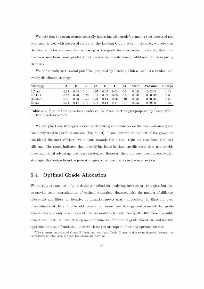
We note that the mean returns generally increasing with grade2, signaling that increased risk

(variance) is met with increased return on the Lending Club platform. However, we note that

the Sharpe ratios are generally decreasing as the grade becomes riskier, indicating that on a

mean-variance basis, lower grades do not necessarily provide enough additional return to justify

their risk.

We additionally test several portfolios proposed by Lending Club as well as a random and

evenly distributed strategy.

Strategy A B C D E F G Mean Variance Sharpe

LC AE 0.28 0.45 0.14 0.07 0.05 0.01 0.0 0.028 0.0003 1.63LC DG 0.17 0.28 0.29 0.14 0.09 0.03 0.0 0.031 0.00037 1.6Random 0.32 0.63 0.53 0.31 0.14 0.06 0.01 0.031 0.00036 1.6Equal 0.14 0.14 0.14 0.14 0.14 0.14 0.14 0.032 0.00046 1.52

Table 5.2: Results testing various strategies. LC refers to strategies proposed by LendingClubin their investors section.

We also plot these strategies, as well as the pure grade strategies on the mean-variance graph

commonly used in portfolio analysis (Figure 5.4). Loans towards the top left of the graph are

considered the most efficient, while loans towards the bottom right are considered the least

efficient. The graph indicates that diversifying loans in these specific cases does not provide

much additional advantage over pure strategies. However, there are very likely diversification

strategies that outperform the pure strategies, which we discuss in the next section.

5.4 Optimal Grade Allocation

We initially set out not only to devise a method for analyzing investment strategies, but also

to provide some approximation of optimal strategies. However, with the number of different

allocations and filters, an iterative optimization proves nearly impossible. To illustrate, even

if we eliminated the ability to add filters to an investment strategy and assumed that grade

allocations could only be multiples of 10%, we would be left with nearly 500,000 different possible

allocations. Thus, we must develop an approximation for optimal grade allocations and use this

approximation as a foundation upon which we can attempt to filter and optimize further.

2The strategy statistics of Grade F Loans are less than Grade G mostly due to randomness because thepercentages of total loans in those two grades are very low

57

To do so, we once again turn to the tenets of modern portfolio theory. We abstract the pure

strategies to assets, such that G is the set of loan grades (A,B,C,D,E,F,G) and rg and σg are

the mean and variance values in Table 5.1 for each g ∈ G. We can then create portfolios of

these assets using a method identical to the one described in Section 5.1.2. These portfolios

have weights wi ∈W, i ∈ G, return rP and variance σ2P . We can then solve the standard convex

minimization problem in portfolio theory, which attempts to minimize variance for a portfolio

subject to a minimum expected rate of return. The minimization optimization outputs the

weights of a portfolio of these assets g ∈ G that successfully minimizes variance for a given rate

of return. We once again assume that the correlation between these assets g is the Basel II

standard, 0.04, and that short positions (negatively weighted assets) and leverage (weights that

sum to > 1) are not allowed. The optimization is modeled as follows [15]

minimizeW

σ2P

subject to∑i∈G

wi = 1

wi > 0 ∀ i ∈ G

rP > r∗

(5.13)

where r∗ is a minimum return defined in the problem. We solved this minimization for various

minimum rates and determined the optimal allocation that minimizes variance for that rate of

return. Since rates of return vary from essentially 2%-4%, we incremented these values by 0.25%.

We found that until 2.75%, the optimal portfolio allocation stays the same, after which there is

a reallocation from safer grades to riskier grades to attempt to meet the required return. We

show the results for this in Table 5.3.

Strategy A B C D E F G Mean Variance Sharpe

2.75% 0.365 0.183 0.127 0.095 0.082 0.072 0.076 0.029 0.00034 1.583.0% 0.295 0.181 0.141 0.11 0.097 0.081 0.094 0.03 0.00037 1.563.25% 0.127 0.178 0.174 0.145 0.133 0.105 0.137 0.033 0.00044 1.563.5% 0.0 0.098 0.198 0.185 0.183 0.13 0.205 0.035 0.00053 1.513.75% 0.0 0.0 0.0 0.031 0.291 0.0 0.678 0.036 0.00064 1.41

Table 5.3: Results of convex optimization problem to determine optimal grade allocations.

Additionally, we plotted the optimal allocations as a purple line in Figure 5.4, in an attempt

58

to model the efficient frontier. In portfolio theory, the efficient frontier is the set of portfolios such

that return cannot be improved without sacrificing variance (i.e. the set of optimal strategies)

[14]. The optimal strategy an investor chooses among this set is solely dependent on his or her

required rate of return.

From Figure 5.4, it is clear that our set of optimal strategies found by the convex optimization

problem does not model the efficient frontier, as pure strategies and the random strategy outper-

form these portfolios. This is largely due to our abstraction of pure strategies to assets. Further

cause for deviation from the actual efficient frontier could be that our assumptions discount the

value of diversification by assuming that correlations across loans and grades are constant. It

could be the case that correlations vary greatly by grade and even subgrade, which would lead

to a completely distinct set of optimal portfolios found by convex optimization. Despite this,

our optimal portfolios are in reality quite close to what would be considered optimal (a curve

outside of the pure strategies) and our optimization approximation has succeeded in that regard.

Further modifications to these strategies by filtering do, in fact, outperform pure strategies, as

we will demonstrate in the next few sections.

5.5 Analysis of Filtering Strategies

The second major decision investors is whether to include filters for various features of the loan in

their investment strategy. While investors can combine filters with grade allocation strategies, in

this initial analysis we first created portfolios of the assets filtered by a given value to isolate the

effect of the filter. Because default probability, mean and return are essentially determined by the

subgrade of the loan, filters essentially improve investment strategy by modifying the particular

subgrade allocation of the portfolio. For the grade allocations of the loans that resulted from the

various filters in this section, please see Appendix B.3. We first filtered by the boolean variables

for home ownership and loan purpose (also including filters for the two term lengths). The results

of this can be seen in Table 5.4.

As shown in the table, only six of the strategies provided meaningful improvements over the

efficiency of a randomized selection of loans, which had a Sharpe ratio of 1.6. Interestingly, the

most meaningful improvements in Sharpe ratio were made by filtering on loans to purchase credit

59

Figure 5.4: Portfolios from Table 5.2 and pure grade strategies plotted. Pseudo-efficient frotierdelimited by purple curve.

60

Variable Mean Variance Sharpe

purpose_educational 0.015 0.00043 0.7home_ownership_none 0.024 0.00092 0.81home_ownership_other 0.02 0.00053 0.87purpose_wedding 0.021 0.00047 0.98purpose_renewable_energy 0.022 0.00047 1.02purpose_small_business 0.026 0.00048 1.19purpose_moving 0.029 0.00048 1.33purpose_car 0.024 0.00032 1.34purpose_house 0.028 0.0004 1.38purpose_other 0.03 0.00046 1.41purpose_major_purchase 0.026 0.00034 1.44purpose_vacation 0.031 0.00045 1.44purpose_medical 0.031 0.00043 1.49home_ownership_rent 0.03 0.0004 1.52term_36 0.029 0.00034 1.55purpose_home_improvement 0.03 0.00034 1.63purpose_debt_consolidation 0.032 0.00037 1.65home_ownership_own 0.032 0.00037 1.66home_ownership_mortgage 0.031 0.00034 1.66purpose_credit_card 0.031 0.00032 1.71term_60 0.036 0.00042 1.76

Table 5.4: Results of filters on boolean variables. Also includes results for filtering based onterm. Portfolio statistics calculated by taking an average of 10 samples of 1000 loans.

cards and loans with a 60 month term. The 60 month filter, in particular, is quite interesting as

it provides meaningful improvement over the best pure strategies. We found that the efficiency of

the 60-month filter has to do with the grade and default time distribution of these loans. Rates

of return are most affected by very negative returns, which happen when a loan defaults in the

first few months of its term. In a 60-month loan, even though overall default rates are higher, the

probability of defaulting in the first few months is slightly less simply because the term is longer.

Though only marginal, this seems to affect the variance of the loans. More importantly, we find

that 60-month loans are typically lower quality than 36-month loans, as shown by Appendix A.3,

which accounts for the higher rate of return. The exposure to a diversified higher risk subgrade

allocation seems to be the most influential in raising the Sharpe ratio of the portfolio, since

default probability is essentially correlated with subgrade due to our prediction heuristic.

Filtering on every value of the non-boolean variables would be impossible, as there are millions

of potential combinations, so we filter on the 25th, 50th and 75th percentile of the values for each

variable. In some cases, the loans had very long-tailed distributions, so we changed the percentiles

61

to the 50th, 90th and 95th. For three of the variables, delinq_2yrs, collections_12_

mths_ex_med and pub_rec, over 95% of the values of these variables were a single value, so

we provided custom values to filter upon. We have shown the values with their corresponding

percentiles in Table 5.5.

Variable Percentile A Percentile B Percentile C

loan_amnt 8000.0(25) 12000.0(50) 20000.0(75)emp_length 3.0(25) 6.0(50) 10.0(75)annual_inc 45000.0(25) 64000.0(50) 89000.0(75)dti 11.0(25) 16.4(50) 22.1(75)delinq_2yrs 1.0(*) 2.0(*) 3.0(*)collections_12_mths_ex_med 0.0(*) 1.0(*) 2.0(*)inq_last_6mths 0.0(50) 2.0(90) 3.0(95)mths_since_last_delinq 0.0(50) 52.0(90) 66.0(95)mths_since_last_record 0.0(50) 37.0(90) 92.0(95)mths_since_last_major_derog 0.0(50) 38.0(90) 56.0(95)pub_rec 0.0(*) 1.0(*) 2.0(*)total_acc 16.0(25) 23.0(50) 31.0(75)open_acc 8.0(25) 10.0(50) 14.0(75)revol_util 0.4(25) 0.6(50) 0.8(75)revol_bal 6524.0(25) 11856.0(50) 20216.0(75)fico_range_low 675.0(25) 690.0(50) 715.0(75)fico_range_high 679.0(25) 694.0(50) 719.0(75)

Table 5.5: Percentile values for variables. Values in parenthesis refer to the percentile of thevariables. A * implies that the values are not percentiles.

We then analyzed portfolios filtered by each of these percentiles and have shown the results

in Table 5.6. For each filter, we filtered by either filtering loans ≥ or ≤ the provided value.

The sign of each filter was chosen to improve the quality of the borrower. In this case, about

half of the filters provided improvements over a randomized strategy, and many provided sub-

stantial increases over pure strategies indicating that filtering for better credit borrowers can be

an effective strategy. The most effective filters used mths_since_last_major_derog and

mths_since_last_record, which seems logical as these variables were both considered effec-

tive by the default classifiers in Chapter 4. As mentioned previously, the success of these filters

indicate that filtering on variables highly predictive of default improves portfolio profitability by

modifying the subgrade allocation of the portfolio. Since default probability ultimately reflects

subgrade, effective filters seem to induce risky but diversified allocations across subgrades that

reduce variance while simultaneously maintaining high expected returns. From the data in Ap-

62

pendix B.3, we see that the improvement in subgrade allocation results from a decrease in both

very safe and very risky subgrades, and a move towards more moderate subgrades with higher

rates of return.

In another interesting result, home_owership, annual_inc and emp_length, which our

default classifiers did not consider effective for predicting default, were considered effective vari-

ables to filter on, while dti, considered effective by the default classifier, was not considered

an effective variable to filter on. This analysis provides insights into the features of the dataset

that the classification never could. If we try to maximize Sharpe ratio, we can see that variables

perhaps considered unimportant by the classifiers could have important consequences for lending

strategies.

Overall, the filters demonstrate that the move towards moderate grade allocations seems

to significantly improve portfolio efficiency, as the nearly strictly decreasing percentage of A-

grade loans in Appendix B.3 indicates. The most effective filters seemed to induce concentrated

investments in B, C, and D loans, with some additional of A and E loans. This overall agrees

with what many P2P investor communities seem to anecdotally know.

63

Variable Percentile Filter Type Mean Variance Sharpe

loan_amnt 25 ≤ 0.028 0.00037 1.47total_acc 25 ≤ 0.029 0.0004 1.48dti 25 ≤ 0.028 0.00035 1.52open_acc 25 ≤ 0.029 0.00037 1.52total_acc 50 ≤ 0.03 0.00038 1.54open_acc 50 ≤ 0.03 0.00037 1.54loan_amnt 50 ≤ 0.029 0.00036 1.55dti 50 ≤ 0.029 0.00035 1.55revol_bal 25 ≤ 0.03 0.00036 1.56dti 75 ≤ 0.03 0.00036 1.57pub_rec 0* ≤ 0.03 0.00036 1.57delinq_2yrs 1* ≤ 0.03 0.00036 1.58inq_last_6mths 95 ≤ 0.03 0.00037 1.58total_acc 75 ≤ 0.03 0.00037 1.58revol_bal 50 ≤ 0.03 0.00037 1.58loan_amnt 75 ≤ 0.03 0.00036 1.59collections_12_mths_ex_med 1* ≤ 0.03 0.00037 1.59open_acc 75 ≤ 0.03 0.00037 1.59delinq_2yrs 2* ≤ 0.03 0.00036 1.6collections_12_mths_ex_med 0* ≤ 0.031 0.00036 1.6collections_12_mths_ex_med 2* ≤ 0.03 0.00036 1.6inq_last_6mths 90 ≤ 0.03 0.00036 1.6mths_since_last_delinq 50 ≥ 0.03 0.00036 1.6mths_since_last_record 50 ≥ 0.031 0.00036 1.6mths_since_last_major_derog 50 ≥ 0.031 0.00037 1.6revol_bal 75 ≤ 0.031 0.00036 1.6fico_range_high 25 ≥ 0.029 0.00034 1.6delinq_2yrs 3* ≤ 0.031 0.00037 1.61pub_rec 1* ≤ 0.031 0.00036 1.61pub_rec 2* ≤ 0.031 0.00036 1.61fico_range_low 50 ≥ 0.028 0.0003 1.61mths_since_last_delinq 90 ≥ 0.032 0.00038 1.62mths_since_last_delinq 95 ≥ 0.032 0.00038 1.62fico_range_low 25 ≥ 0.03 0.00033 1.62fico_range_high 50 ≥ 0.028 0.0003 1.62emp_length 25 ≥ 0.031 0.00036 1.63fico_range_low 75 ≥ 0.025 0.00024 1.63fico_range_high 75 ≥ 0.025 0.00024 1.63annual_inc 50 ≥ 0.031 0.00035 1.64revol_util 25 ≤ 0.028 0.00028 1.64annual_inc 25 ≥ 0.031 0.00036 1.65revol_util 75 ≤ 0.03 0.00034 1.65inq_last_6mths 50 ≤ 0.03 0.00033 1.66emp_length 50 ≥ 0.032 0.00036 1.67revol_util 50 ≤ 0.03 0.00031 1.67annual_inc 75 ≥ 0.031 0.00034 1.69emp_length 75 ≥ 0.032 0.00036 1.7mths_since_last_record 95 ≥ 0.033 0.00037 1.74mths_since_last_record 90 ≥ 0.036 0.00037 1.85mths_since_last_major_derog 95 ≥ 0.037 0.00037 1.91mths_since_last_major_derog 90 ≥ 0.037 0.00037 1.92

Table 5.6: Results of filters on variables. Percentiles refers to the values in the above table,unless denoted by a *, in which they refer to a value, not a percentile. Filter type refers towhether the loans were filtered by taking ≤ or ≥ than the value in question. Portfolio statisticscalculated by taking an average of 10 samples of 1000 loans.

64

5.6 Optimal Filters

We combine this framework for analyzing filters with our previous work on optimal grade al-

location. Let’s assume that an investor has a minimum required rate of return of 2.75%. The

investor would then choose the 2.75% strategy from Table 5.3, which would return him or her

a 2.9% return with a Sharpe Ratio of 1.58. We seek to boost this Sharpe ratio by filtering.

We filter based on each of the values detailed in Section 5.5. However, we find that in many

cases, filters conflict with the grade allocation. For example, our strategy requires 7.6% G-rated

loans. If we were to filter to require a FICO Score of 650, we would find it nearly impossible to

find 7.6% loans in a diversified portfolio, as hardly any G-Rated loans have FICO Scores high

enough. In Tables 5.7 and 5.8, we show the results of filtering while also maintaining the grade

allocation from Table 5.3. We note that several of the filters from the tables in Section 5.5 are

missing, as these filters conflicted with the required grade allocation. Overall, the types of filters

that improve Sharpe Ratio tend to be similar to the ones from above. In this case, the grade

allocation is maintained, but the filters induce modifications to the subgrade allocations across

different grades. For instance, we might see riskier A-grade loans (i.e. subgrades A4 and A5)

but safer F and G rated loans, which seem to improve overall portfolio probability. Even while

maintaining grade allocations, filtering allows for significant outperformance of pure strategies.

Variable Mean Variance Sharpe

purpose_small_business 0.024 0.00037 1.26term_36 0.027 0.00036 1.43purpose_other 0.028 0.00036 1.45home_ownership_rent 0.028 0.00035 1.52purpose_credit_card 0.029 0.00033 1.6purpose_debt_consolidation 0.029 0.00034 1.6home_ownership_mortgage 0.03 0.00033 1.65home_ownership_own 0.03 0.00033 1.66term_60 0.03 0.0003 1.75

Table 5.7: Results of filters on boolean variables for optimal portfolio found by convex op-timization. Also includes results for filtering based on term. Portfolio statistics calculated bytaking an average of 10 samples of 1000 loans.

65

Variable Percentile Filter Type Mean Variance Sharpe

total_acc 25 ≤ 0.028 0.00035 1.48open_acc 25 ≤ 0.028 0.00034 1.49dti 25 ≤ 0.028 0.00034 1.5dti 50 ≤ 0.028 0.00034 1.53total_acc 50 ≤ 0.028 0.00034 1.53open_acc 50 ≤ 0.028 0.00034 1.53dti 75 ≤ 0.028 0.00034 1.54revol_bal 25 ≤ 0.028 0.00034 1.54pub_rec 0* ≤ 0.029 0.00034 1.55open_acc 75 ≤ 0.028 0.00034 1.55revol_bal 50 ≤ 0.029 0.00034 1.55delinq_2yrs 1* ≤ 0.029 0.00034 1.56inq_last_6mths 95 ≤ 0.029 0.00034 1.56pub_rec 1* ≤ 0.029 0.00034 1.56revol_bal 75 ≤ 0.029 0.00034 1.56delinq_2yrs 2* ≤ 0.029 0.00034 1.57collections_12_mths_ex_med 0* ≤ 0.029 0.00034 1.57collections_12_mths_ex_med 1* ≤ 0.029 0.00034 1.57mths_since_last_delinq 50 ≥ 0.029 0.00034 1.57mths_since_last_delinq 90 ≥ 0.029 0.00034 1.57total_acc 75 ≤ 0.029 0.00034 1.57loan_amnt 50 ≤ 0.029 0.00034 1.58collections_12_mths_ex_med 2* ≤ 0.029 0.00034 1.58inq_last_6mths 50 ≤ 0.029 0.00033 1.58inq_last_6mths 90 ≤ 0.029 0.00033 1.58mths_since_last_record 50 ≥ 0.029 0.00034 1.58pub_rec 2* ≤ 0.029 0.00034 1.58delinq_2yrs 3* ≤ 0.029 0.00034 1.59mths_since_last_major_derog 50 ≥ 0.029 0.00034 1.59loan_amnt 75 ≤ 0.029 0.00034 1.6fico_range_high 25 ≥ 0.029 0.00033 1.6annual_inc 25 ≥ 0.029 0.00033 1.61annual_inc 50 ≥ 0.029 0.00033 1.61revol_util 25 ≤ 0.029 0.00032 1.61fico_range_low 25 ≥ 0.029 0.00034 1.61emp_length 25 ≥ 0.03 0.00033 1.62revol_util 50 ≤ 0.029 0.00033 1.62fico_range_low 50 ≥ 0.029 0.00033 1.62fico_range_high 50 ≥ 0.029 0.00033 1.62revol_util 75 ≤ 0.03 0.00033 1.63emp_length 50 ≥ 0.03 0.00033 1.64annual_inc 75 ≥ 0.03 0.00033 1.64emp_length 75 ≥ 0.03 0.00033 1.67mths_since_last_record 90 ≥ 0.032 0.00033 1.76mths_since_last_major_derog 90 ≥ 0.034 0.00032 1.88

Table 5.8: Results of filters on optimal portfolio found by convex optimization. Percentilesrefers to the values in the above table, unless denoted by a *, in which they refer to a value, nota percentile. Filter type refers to whether the loans were filtered by taking ≤ or ≥ than the valuein question. Portfolio statistics calculated by taking an average of 10 samples of 1000 loans.

66

5.7 Introduction of Novel Analysis Tool

Since an investment strategy on Lending Club is defined by a choice of grade allocation and

filters, we must find a way to model both of these choices simultaneously. We have shown

methods on optimizing grade allocation, filtering and filtering while simultaneously maintaining

a specific grade allocation. The reality of LendingClub investment however, is that the actual

decisions made are even more complex. In the Automated Investment Tool, an investor can

choose multiple filters in combination with a grade allocation, which is quite difficult to analyze.

To rectify this, and since analyzing every possible filter and grade allocation is infeasible, to

analyze the joint decision, the author built a web application.

In the web application, one can filter on any value of any feature and input any allocation

and visualize the mean, variance and Sharpe ratio for the investment strategy. The application

is located at http://kunalmehta-thesis-dev.us-west-2.elasticbeanstalk.com.

Please note that using filtering and grade allocation strategies from this thesis on the application

may result in slightly different values of mean, variance and Sharpe ratio. This is primarily due

to the fact that statistics on the application are not calculated as an average of ten random

samples of one thousand loans but rather, to save time in displaying analysis output, are simply

the values calculated from a single random sample of one thousand loans.

67

Chapter 6

Conclusion

In the introduction, our two primary goals were to determine a framework for analyzing in-

vestments on Online P2P Marketplaces (specifically LendingClub) and thereby develop a set of

optimal practices and, second, to analyze the drivers of default on these marketplaces, focusing

our efforts on determining the value of the FICO Score and the assigned subgrade/interest rate.

We first attempted to understand how various features affected propensity to default by splitting

the features into categories and then combining these categories into variable sets, to understand

the marginal additions in prediction accuracy gained by additional features. We found that with-

out the LendingClub assigned subgrade, we can at best predict 67% of the loans accurately, with

the most important features being the amount of the loan, debt-to-income ratio of the borrower

and several credit related features. We can achieve this 67% prediction rate either by only using

the FICO Score or by using most of the other variables in the dataset, including information

about the loan, the borrower and the borrower’s credit history. Furthermore, we can achieve ac-

curacies of approximately 61% just from knowing the loan’s amount and purpose. This indicates

that the FICO score as a measure of propensity to default is quite weak, as it doesn’t provide

an improvement of more than 5% in accuracy. On the other hand, the LendingClub assigned

subgrade and interest rate, by themselves, result in an accuracy of 86%, an improvement of 20%

over any other combination of features in the dataset. The resulting improvement in accuracy

seems to be a consequence of improved prediction techniques as well as additional data, quite

68

possibly of the borrower’s location and more detailed credit history. From this feature analy-

sis, we found that the optimal subset for predicting defaults consists solely of the LendingClub

assigned subgrade and interest rate, with the optimal classifier being the decision tree.

Using this optimal subset and modifying the hitherto balanced dataset to reflect the under-

lying 10% base default rate of LendingClub loans, we derived a probability of default for each

loan, which we then used to determine mean and variance. Combining these loans into portfo-

lios, we were able to analyze various strategies by developing a framework inspired by modern

portfolio theory and expected value, viewing a strategy as the purchase of a portfolio of loans

held to maturity. Our analysis of investment strategies, specifically grade allocations and filters,

resulted in a number of conclusions. First, we found that the expected increase in return at the

expense of variance exists in LendingClub grades, with the riskier grades providing additional

returns. However, the Sharpe ratio of a portfolio of loans using these pure strategies decreases as

the loans become riskier, indicating that the additional return of riskier D-G grade loans may not

be sufficient to justify the additional variance, largely because loans tend to default early and a

higher default rate increases the likelihood of significant losses. We used convex optimization to

attempt to discover the efficient frontier of LendingClub investment strategies and our approxi-

mation, while not as optimal as many naive strategies, did provide a pseudo-optimal foundation

by which to analyze additional optimizations to investment strategy, most notably filters.

In our analysis of filters, we found that typically, variables we found in our analysis of default

to be highly predictive of default tended to be the most effective features, as filtering on these

features allows a reduction in default rate while simultaneously exposing the investor to a more

efficient allocation of subgrades than would otherwise be possible. Interestingly, we found that

variables previously considered to be not predictive of default, such as annual income, home

ownership and employment length, features by and large considered important by traditional

financial intermediaries but unimportant by our loan classification algorithms, tended to addi-

tionally be quite effective as features to filter upon, indicating that these traditionally important

predictors of default do provide value. These filters were effective regardless of grade alloca-

tion, unless of course the filter conflicts with the intended allocation, resulting in an impossible

investment mandate.

While we are wary generalizing our results here to be applicable to other investment platforms

69

and the personal credit marketplace more generally, our data does raise interesting questions

regarding lending strategies more generally. First, with the rise of alternative platforms such

as Upstart that in some cases do not require credit scores or complex verification schemes, our

analysis seems to suggest that acquiring additional credit information without the requisite social

data and complex prediction techniques may not provide very much marginal value over simply

knowing basic information about the loan request and the borrower. Second, we found that by

and large, investing in the ”middle” of the loan risk spectrum seems to generally provide the best

risk-adjusted return, and that filtering to attempt to reduce default rates is an effective strategy

as well, confirming what many P2P investors seem to intrinsically know but not exhaustively

investigate.

Perhaps most importantly, we argue that meaningful analysis can be done on P2P loans

without looking at NAR, APR and the various other complex and often perplexing metrics that

characterize the space. Instead, one of the simplest financial tools, the mean-variance analysis and

corresponding Sharpe ratio can provide significant value to understanding how the marketplace

functions. Further, this expected value approach additionally provides value in terms of deciding

between investment strategies by using a forward-looking, instead of only retrospective, measure

of investment returns, another point of obfuscation of many current LendingClub profitability

metrics.

Future work in this vein could focus on determining loan correlations in P2P Lending and

accounting for late fees, service fees and the variety of complex interaction that underlie our

simplified approach. Additionally, analyses of this sort utilizing different platforms, such as

Prosper, OnDeck and Upstart, could prove immensely valuable.

To end on a more philosophical note, our study had primary motivations. First, we wanted

to promote the study of P2P Lending in a rigorous academic setting. Current ”literature”

on the topic, as we discussed in Chapter 2, primarily consists of blogs which often devolve

into arguments without evidence or substance aside from the anecdotal. With more analytical

academic literature on the subject, P2P Lending might become an alternative asset used by

millions of Americans. This leads into our second major motivation for developing this project.

We hoped to simplify the idea of P2P investing, especially through our application described

in Chapter 5 that models investment decisions in an easy to understand visualization. We

70

attempted to demonstrate how one could view these P2P loans as streams of payments subject

to probability, fundamentally equivalent to a bond or a stock.

Despite the incredible growth in P2P Lending, many Americans still hesitate to invest on

these platforms, perhaps due to fear, barriers to entry or perceived complexity [1]. This thesis,

above all, seeks to dispel the idea that LendingClub investment strategies are fundamentally

distinct from the stock market or from investing in bonds. They are not. Like bonds or like

stocks, they simply reflect an expected stream of payments which may or may not actualize, and

our framework treats them as such.

In conclusion, this thesis does not intend to encourage readers to invest their life savings in a

60-month filtered equal allocation or even, as many have done, to invest in online P2P Lending

as an alternate investment strategy to benefit the entirety of one’s portfolio. Rather, we simply

wish to demonstrate a framework for analysis and a description of the feature set that could be

used to better understand and appreciate this groundbreaking investment platform. The new

age of personal credit has arrived, and we would be wise to at least take it seriously.

71

Appendices

72

Appendix A

Additional Information

A.1 Application Screenshots

Figure A.1: Screenshot of Application

Figure A.2: Screenshot of Application

73

A.2 LendingClub Screenshots

Figure A.3: Screenshot of Loan Browser [13]

Figure A.4: Screenshot of Automated Investing Service [13]

74

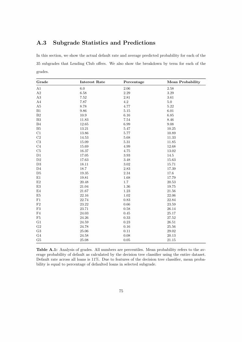
A.3 Subgrade Statistics and Predictions

In this section, we show the actual default rate and average predicted probability for each of the

35 subgrades that Lending Club offers. We also show the breakdown by term for each of the

grades.

Grade Interest Rate Percentage Mean Probability

A1 6.0 2.06 2.58A2 6.58 2.29 3.29A3 7.52 2.81 3.61A4 7.87 4.2 5.0A5 8.78 4.77 5.22B1 9.86 5.15 6.01B2 10.9 6.16 6.85B3 11.83 7.54 8.46B4 12.65 6.99 9.08B5 13.21 5.47 10.25C1 13.86 5.77 10.89C2 14.53 5.68 11.33C3 15.09 5.31 11.85C4 15.69 4.99 12.68C5 16.37 4.75 13.02D1 17.05 3.93 14.5D2 17.63 3.48 15.63D3 18.11 3.02 15.71D4 18.7 2.83 17.39D5 19.35 2.34 17.6E1 19.81 1.68 17.79E2 20.48 1.7 20.53E3 21.04 1.36 19.75E4 21.67 1.23 21.56E5 22.16 1.02 22.06F1 22.74 0.83 22.84F2 23.22 0.66 23.59F3 23.71 0.58 26.14F4 24.03 0.45 25.17F5 24.26 0.33 27.52G1 24.59 0.23 26.51G2 24.78 0.16 25.56G3 25.06 0.11 29.02G4 24.58 0.08 20.13G5 25.08 0.05 21.15

Table A.1: Analysis of grades. All numbers are percentiles. Mean probability refers to the av-erage probability of default as calculated by the decision tree classifier using the entire dataset.Default rate across all loans is 11%. Due to features of the decision tree classifier, mean proba-bility is equal to percentage of defaulted loans in selected subgrade.

75

Grade 36 months 60 months

A1 1.0 0.0A2 1.0 0.0A3 1.0 0.0A4 0.98 0.02A5 0.92 0.08B1 0.87 0.13B2 0.88 0.12B3 0.84 0.16B4 0.8 0.2B5 0.85 0.15C1 0.77 0.23C2 0.71 0.29C3 0.65 0.35C4 0.58 0.42C5 0.59 0.41D1 0.6 0.4D2 0.6 0.4D3 0.58 0.42D4 0.49 0.51D5 0.45 0.55E1 0.38 0.62E2 0.34 0.66E3 0.29 0.71E4 0.25 0.75E5 0.26 0.74F1 0.23 0.77F2 0.18 0.82F3 0.22 0.78F4 0.16 0.84F5 0.12 0.88G1 0.1 0.9G2 0.09 0.91G3 0.07 0.93G4 0.07 0.93G5 0.05 0.95

Table A.2: Analysis of terms of various grades. All numbers are percentiles.

76

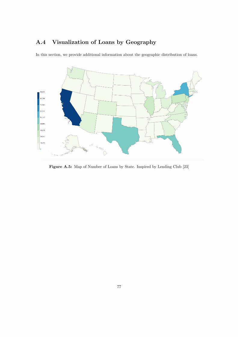
A.4 Visualization of Loans by Geography

In this section, we provide additional information about the geographic distribution of loans.

Figure A.5: Map of Number of Loans by State. Inspired by Lending Club [23]

77

A.5 Pseudocode for Ranked Optimal Subset Algorithm

In this section we provide pseudocode for the Algorithm descriped in Chapter 4 and introduced

in Friedmant, et. al. [34]. Note that aS(X) refers to the cross validation accuracy of a classifier

using subset S as the features of loans X.Data: feature set Sj , set of training loans X, set of training statuses y

Optimal ranked subset of features and accuracies O = {};

Best score b = 0;

Qj = Sj ;

for variable v ∈ Sj do

set of feature subsets and accuracies V = {};

for variable w ∈ Qj do

temp subset T = O + v;

V = V + (aT (X), T );

end

subset with max score from V = B;

max score b2;

best additional variable added x = B −O;

Qj = Qj − x;

if aB(X) > b and Qj = ∅ then

b = b2;

O = O + x;

return O

end

else if aB(X) < b or Qj = ∅ then

return O

end

else

b = b2;

O = O + x;

end

end

Algorithm 1: Returns ranked optimal subset O of features from Si

78

A.6 Additional Classification Methods

In this section, we briefly discuss additional methods that we used to classify loans.1

A.6.1 Perceptron Algorithm

One way to look at binary classification is to consider X as a set of points in f -dimensional

space, where f , again, is the number of features in the dataset. The task of binary classification

then, could be rewritten as finding a hyperplane that optimally separates the points in the two

classes. Following from Friedman, we reclassify Y = {0, 1} as Y = {−1, 1} and our hyperplane

takes the form [34]

y = xTi β + β0. (A.1)

Then, for all responses where yi = 1 that are misclassified, we must have that y < 0 and vice

versa. The perceptron attempts to minimize misclassification by updating β and β0. It defines

a quantity to be minimized [34]

∆(β, β0) = −∑i∈M

yi(xTi β + β0), (A.2)

where M indexes the set of misclassified points. The perceptron minimizes the above by

continuously iterating through each point and updating the values [34]

(β

β0

)+

(yixiyi

)→(β

β0

), (A.3)

until there are no longer any misclassified points. For full explanation see Friedman [34]. We

can show that if classes are linearly separable, eventually the algorithm will converge, though

often classes are not linearly separable [34]. In the implementation used, we set a maximum

number of iterations (5), and thus by Equation A.1, we can see that the algorithm has runtime

O(nf2), similar to a regression.

1Again, most information comes from Friedman.

79

A.6.2 Support Vector Machine

Support Vector Machines are extensions of the use of separating hyperplanes for classification.

They are much more complex than the other techniques used. For simplicity, we have only

provided a brief theoretical overview of the SVM but provided references to additional materials.

For our two-class problem, where yi ∈ {0, 1}, we have seen that a logical way to classify inputs

would be to find an optimally separating hyperplane (xTi β+β0) that maximizes the margin, M ,

between the training points in classes yi = 0 and yi = 1 [34]. This optimization problem can be

written as [34]

minβ,β0,||β||=1

M

subject to yi(xtiβ + β0) ≥M

(A.4)

The novel addition of the SVM is to allow for some points to be on the wrong side of the

margin. [34] We define slack variables for each input i, εi s.t. ∀i, εi ≥ 0,∑i εi ≤ C [34]. The

value εi, thus, is the proportional amount by which the prediction is on the wrong side of its

margin. Thus, we have [34]

minβ,β0,||β||=1

M

subject to yi(xtiβ + β0) ≥M − εi

(A.5)

For additional information on calculating β please see Friedman [34]. For the support vector

machine, we found that no other variable provides an increase in accuracy above the standard

deviation of the accuracy of the default parameters in the implementation of the support vector

we utilized: C = 1.0, ε = 0.1. Support vector machine runtime is O(n3), and as you can

expect, runtime was prohibitively complex and we again used bagging to reduce actual (but not

asymptotic) runtime [46]. The expected decrease in variance at the expense of bias was noted,

but no tangible impacts on the predictions were seen.

80

A.6.3 Boosted Decision Tree

For a simple decision tree, let’s assume that instead of square error, we simply used absolute

accuacy in that the error of a classifier was simply, [34]

e =1

N

N∑i=1

|yi − yi|, (A.6)

assuming, of course, that y ∈ {0, 1}. In other words, we are taking the percentage of the

indicator variables such that yi 6= yi. Our classifier seeks to minimize this error. Now suppose

we weighted each point differently, such that [34]

e =

N∑i=1

wi|yi − yi|, (A.7)

and all the wi summed to 1. A boosted tree, specifically the formulation AdaBoost (which

we use), seeks to iteratively reweight these weights, at each iteration increasing the weight of

misclassified points and decreasing the weight of correctly classified points. Thus the decision

tree is forced to focus on points that are difficult to predict, in theory increasing the accuracy

of the prediction [17]. In many cases boosting provides a tremendous advantage over ”weak”

learning techniques [17]. Since the number of iterations is a constant that is pre-determined,

runtime is stil O(fn log n) [16].

81

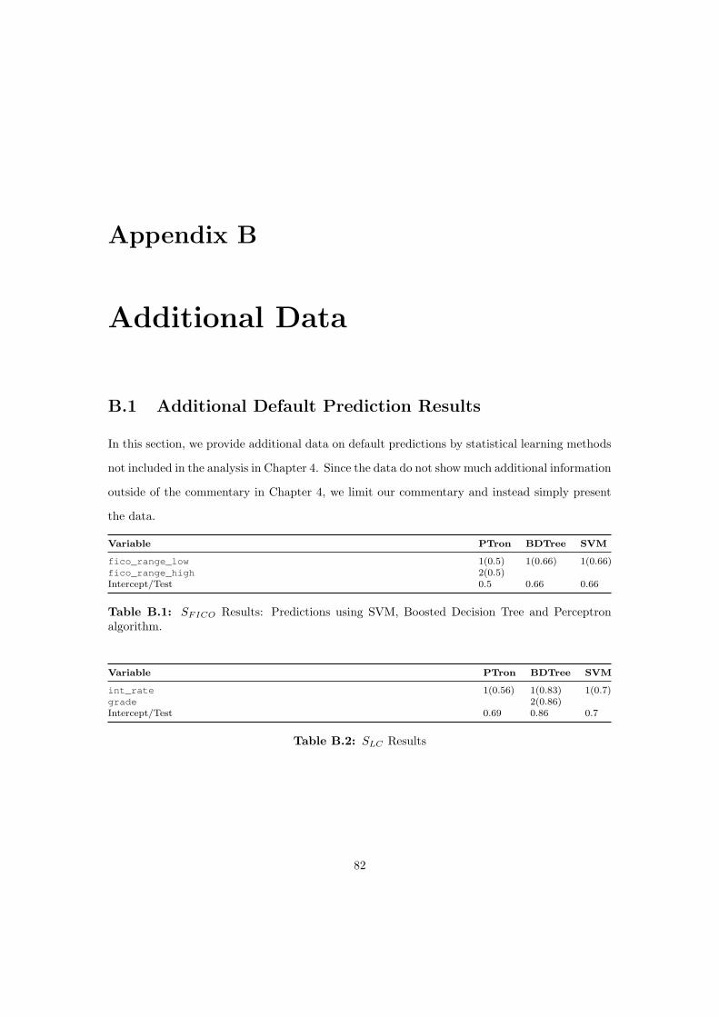
Appendix B

Additional Data

B.1 Additional Default Prediction Results

In this section, we provide additional data on default predictions by statistical learning methods

not included in the analysis in Chapter 4. Since the data do not show much additional information

outside of the commentary in Chapter 4, we limit our commentary and instead simply present

the data.

Variable PTron BDTree SVM

fico_range_low 1(0.5) 1(0.66) 1(0.66)fico_range_high 2(0.5)Intercept/Test 0.5 0.66 0.66

Table B.1: SFICO Results: Predictions using SVM, Boosted Decision Tree and Perceptronalgorithm.


int_rate 1(0.56) 1(0.83) 1(0.7)grade 2(0.86)Intercept/Test 0.69 0.86 0.7

Table B.2: SLC Results

82


loan_amnt 1(0.63) 1(0.63)purpose_debt_consolidation 1(0.51)term 2(0.64) 2(0.64)Intercept/Test 0.5 0.64 0.64

Table B.3: S1 Results


emp_length 2(0.62)dti 1(0.54) 1(0.57) 1(0.61)home_ownership_rent 2(0.57)Intercept/Test 0.5 0.58 0.61



mths_since_last_major_derog 1(0.53) 2(0.6) 3(0.64)pub_rec 3(0.6)open_acc 2(0.62)revol_util 1(0.58) 1(0.6)Intercept/Test 0.5 0.61 0.64



loan_amnt 1(0.63) 1(0.63)purpose_renewable_energy 3(0.64)term 2(0.58) 2(0.64)dti 1(0.54) 2(0.64)Intercept/Test 0.59 0.64 0.64



loan_amnt 1(0.63) 1(0.63)term 3(0.67) 3(0.67)mths_since_last_major_derog 1(0.53) 2(0.66) 2(0.66)Intercept/Test 0.5 0.67 0.67



mths_since_last_record 3(0.6)mths_since_last_major_derog 2(0.58) 2(0.6) 2(0.64)pub_rec 4(0.66)revol_util 1(0.58) 3(0.66)dti 1(0.54) 1(0.61)Intercept/Test 0.5 0.6 0.66


83


loan_amnt 1(0.63) 1(0.63)term 3(0.67) 3(0.67)dti 1(0.54)mths_since_last_major_derog 2(0.58) 2(0.66) 2(0.66)Intercept/Test 0.5 0.67 0.67



purpose_credit_card 3(0.72)mths_since_last_delinq 2(0.64)mths_since_last_major_derog 2(0.71)int_rate 1(0.56) 1(0.83) 1(0.7)grade 2(0.86)Intercept/Test 0.65 0.86 0.71


84

B.2 FICO Comparison Results

In this section, we provide additional data on the margial value of the FICO scores using the

most predictive model, the decision tree.

Variable Without FICO With FICO

int_rate 1(0.83) 1(0.83)grade 2(0.86) 2(0.86)test 0.86 0.86

Table B.11: SLC Results: FICO Comparison


loan_amnt 1(0.63) 2(0.67)term 2(0.64)fico_range_low 1(0.66)test 0.64 0.67

Table B.12: S1 Results: FICO Comparison


dti 1(0.57)fico_range_low 1(0.66)test 0.58 0.66



mths_since_last_major_derog 2(0.6)pub_rec 3(0.6)open_acc 2(0.66)revol_util 1(0.58)fico_range_low 1(0.66)test 0.6 0.67



loan_amnt 1(0.63) 2(0.67)term 2(0.64)fico_range_low 1(0.66)test 0.64 0.67


85


loan_amnt 1(0.63) 2(0.67)term 3(0.67)mths_since_last_major_derog 2(0.66) 3(0.68)fico_range_low 1(0.66)test 0.67 0.67



mths_since_last_major_derog 2(0.6)pub_rec 3(0.6)open_acc 2(0.66)revol_util 1(0.58)fico_range_low 1(0.66)test 0.6 0.67



loan_amnt 1(0.63) 2(0.67)term 3(0.67)mths_since_last_major_derog 2(0.66) 3(0.68)fico_range_low 1(0.66)test 0.67 0.67



int_rate 1(0.83) 1(0.83)grade 2(0.86) 2(0.86)test 0.86 0.86


86

B.3 Grade Allocations for Filtering Strategies

In this section, we provide data on the grade allocations that resulted from various filters.

Variable Percentile Filter Type A B C D E F G

fico_range_low 75 ≥ 0.47 0.33 0.14 0.04 0.01 0.0 0.0fico_range_high 75 ≥ 0.47 0.33 0.14 0.04 0.01 0.0 0.0revol_util 25 ≤ 0.35 0.32 0.19 0.09 0.04 0.01 0.0fico_range_low 50 ≥ 0.28 0.37 0.21 0.09 0.04 0.01 0.0fico_range_high 50 ≥ 0.28 0.37 0.21 0.09 0.04 0.01 0.0annual_inc 75 ≥ 0.21 0.29 0.23 0.14 0.08 0.03 0.01revol_util 50 ≤ 0.25 0.34 0.23 0.11 0.04 0.02 0.0dti 25 ≤ 0.22 0.32 0.24 0.13 0.06 0.02 0.01inq_last_6mths 50 ≤ 0.21 0.36 0.24 0.12 0.05 0.02 0.0annual_inc 50 ≥ 0.19 0.3 0.25 0.15 0.08 0.03 0.01dti 50 ≤ 0.2 0.32 0.25 0.14 0.06 0.02 0.01revol_util 75 ≤ 0.2 0.34 0.25 0.13 0.06 0.02 0.0fico_range_low 25 ≥ 0.21 0.35 0.25 0.12 0.05 0.02 0.0fico_range_high 25 ≥ 0.21 0.35 0.25 0.12 0.05 0.02 0.0loan_amnt 25 ≤ 0.18 0.34 0.26 0.16 0.05 0.01 0.0loan_amnt 75 ≤ 0.17 0.34 0.26 0.15 0.05 0.02 0.0annual_inc 25 ≥ 0.17 0.31 0.26 0.15 0.07 0.03 0.01dti 75 ≤ 0.18 0.32 0.26 0.15 0.07 0.03 0.01delinq_2yrs 1* ≤ 0.17 0.31 0.26 0.15 0.07 0.03 0.01delinq_2yrs 2* ≤ 0.16 0.31 0.26 0.15 0.07 0.03 0.01delinq_2yrs 3* ≤ 0.16 0.31 0.26 0.16 0.07 0.03 0.01collections_12_mths_ex_med 0* ≤ 0.16 0.31 0.26 0.16 0.07 0.03 0.01collections_12_mths_ex_med 1* ≤ 0.16 0.31 0.26 0.16 0.07 0.03 0.01collections_12_mths_ex_med 2* ≤ 0.16 0.31 0.26 0.16 0.07 0.03 0.01inq_last_6mths 90 ≤ 0.17 0.32 0.26 0.15 0.07 0.03 0.01inq_last_6mths 95 ≤ 0.16 0.32 0.26 0.15 0.07 0.03 0.01mths_since_last_delinq 50 ≥ 0.16 0.31 0.26 0.16 0.07 0.03 0.01mths_since_last_record 50 ≥ 0.16 0.31 0.26 0.16 0.07 0.03 0.01mths_since_last_major_derog 50 ≥ 0.16 0.31 0.26 0.16 0.07 0.03 0.01pub_rec 0* ≤ 0.18 0.31 0.26 0.15 0.07 0.03 0.01pub_rec 1* ≤ 0.16 0.31 0.26 0.15 0.07 0.03 0.01pub_rec 2* ≤ 0.16 0.31 0.26 0.16 0.07 0.03 0.01open_acc 75 ≤ 0.16 0.32 0.26 0.16 0.07 0.03 0.01revol_bal 25 ≤ 0.19 0.3 0.26 0.16 0.06 0.02 0.0loan_amnt 50 ≤ 0.18 0.35 0.27 0.15 0.05 0.01 0.0emp_length 25 ≥ 0.16 0.31 0.27 0.16 0.07 0.03 0.01emp_length 50 ≥ 0.16 0.31 0.27 0.16 0.07 0.03 0.01emp_length 75 ≥ 0.16 0.31 0.27 0.16 0.07 0.03 0.01mths_since_last_delinq 95 ≥ 0.13 0.32 0.27 0.17 0.08 0.03 0.01total_acc 50 ≤ 0.15 0.32 0.27 0.16 0.07 0.03 0.01total_acc 75 ≤ 0.16 0.32 0.27 0.16 0.07 0.03 0.01open_acc 25 ≤ 0.16 0.31 0.27 0.16 0.07 0.03 0.01open_acc 50 ≤ 0.16 0.32 0.27 0.16 0.07 0.03 0.01revol_bal 50 ≤ 0.16 0.32 0.27 0.16 0.06 0.02 0.0revol_bal 75 ≤ 0.16 0.32 0.27 0.16 0.07 0.03 0.01mths_since_last_delinq 90 ≥ 0.12 0.32 0.28 0.17 0.08 0.03 0.01total_acc 25 ≤ 0.13 0.31 0.28 0.18 0.07 0.03 0.01mths_since_last_record 95 ≥ 0.07 0.36 0.3 0.16 0.07 0.03 0.01mths_since_last_major_derog 90 ≥ 0.07 0.3 0.31 0.19 0.08 0.03 0.01mths_since_last_record 90 ≥ 0.05 0.33 0.32 0.18 0.08 0.03 0.01mths_since_last_major_derog 95 ≥ 0.07 0.3 0.32 0.19 0.08 0.03 0.01

Table B.20: Grade allocations of filtering strategies.

87

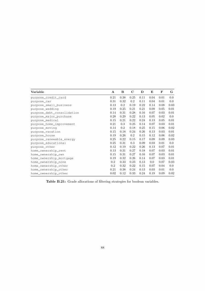
Variable A B C D E F G

purpose_credit_card 0.21 0.38 0.25 0.11 0.04 0.01 0.0purpose_car 0.31 0.32 0.2 0.11 0.04 0.01 0.0purpose_small_business 0.13 0.2 0.19 0.22 0.14 0.08 0.03purpose_wedding 0.19 0.25 0.21 0.21 0.09 0.05 0.01purpose_debt_consolidation 0.14 0.31 0.28 0.16 0.07 0.03 0.01purpose_major_purchase 0.28 0.29 0.22 0.13 0.05 0.02 0.0purpose_medical 0.15 0.21 0.22 0.24 0.13 0.05 0.01purpose_home_improvement 0.21 0.3 0.25 0.14 0.07 0.03 0.01purpose_moving 0.14 0.2 0.18 0.25 0.15 0.06 0.02purpose_vacation 0.15 0.18 0.24 0.26 0.13 0.03 0.01purpose_house 0.19 0.26 0.2 0.15 0.12 0.06 0.02purpose_renewable_energy 0.25 0.22 0.15 0.17 0.09 0.09 0.03purpose_educational 0.25 0.31 0.3 0.09 0.03 0.01 0.0purpose_other 0.12 0.19 0.22 0.26 0.13 0.07 0.01home_ownership_rent 0.13 0.31 0.27 0.18 0.07 0.03 0.01home_ownership_own 0.15 0.31 0.27 0.16 0.07 0.03 0.01home_ownership_mortgage 0.19 0.32 0.26 0.14 0.07 0.03 0.01home_ownership_none 0.2 0.33 0.23 0.13 0.0 0.07 0.03home_ownership_other 0.2 0.32 0.22 0.15 0.07 0.04 0.0home_ownership_other 0.21 0.38 0.24 0.13 0.03 0.01 0.0home_ownership_other 0.02 0.12 0.33 0.24 0.19 0.09 0.02

Table B.21: Grade allocations of filtering strategies for boolean variables.

88

Bibliography

[1] 7 Problems that Keep P2P Lending a Niche Investment.http://www.lendingmemo.com/peer-lending-problems/.

[2] Current treasury rates. https://www.treasury.gov/resource-center/data-chart-center/interest-rates/Pages/TextView.aspx?data=yield.

[3] How to calculate loan repayment lending club amortization formula.https://www.youtube.com/watch?v=FJqt8F5NB10.

[4] Investopedia Guide to Corporate Finance. http://www.investopedia.com/walkthrough/corporate-finance/4/return-risk/expected-return.aspx.

[5] Lendacademy forums: Worst month yet. http://www.lendacademy.com/forum/index.php?topic=3551.0.

[6] Lending Club: Download Data. https://www.lendingclub.com/info/download-data.action.

[7] Lending Club: FAQs for New Investors. https://www.lendingclub.com/public/investing-faq.action.

[8] Lending Club: How Long Does It Take To Get My Loan.http://kb.lendingclub.com/borrower/articles/Borrower/How-long-does-it-take-to-get-my-loan.

[9] Lending Club: How We Measure Net Annualized Return.

[10] Lending Club Personal Loan Application. https://www.youtube.com/watch?v=dUv7CX-37Yc.

[11] Lending Club Trading Platform. https://www.lendingclub.com/foliofn/aboutTrading.action.

[12] Lending Club: What Do The Different Note Statuses Mean.http://kb.lendingclub.com/investor/articles/Investor/What-do-the-different-Note-statuses-mean/.

[13] Lending Club: What We Do. https://www.lendingclub.com/public/about-us.action.

[14] Modern portfolio theory and the efficient frontier. https://www.smart401k.com/resource-center/advanced-investing/modern-portfolio-theory-and-the-efficient-frontier.

[15] Portfolio Optimization with Python. https://wellecks.wordpress.com/2014/03/23/portfolio-optimization-with-python/.

[16] SciKit Learn: Decision Trees. http://scikit-learn.org/stable/modules/tree.html.

89

[17] SciKit Learn: Ensemble Methods. http://scikit-learn.org/stable/modules/ensemble.html.

[18] SciKit Learn: Linear Regression. http://scikit-learn.org/stable/modules/linear model.html.

[19] SciKit Learn: Nearest Neighbors. http://scikit-learn.org/stable/modules/neighbors.html.

[20] Spdr s&p 500 etf (spy). https://finance.yahoo.com/q/rk?s=SPY+Risk.

[21] Simple Filters for Investing in Lending Club and Prosper.http://www.writeyourownreality.com/lending-club/simple-filters-for-investing-lending-club-prosper/, February 2014.

[22] Lendingclub 10-k. http://ir.lendingclub.com/Cache/33047201.pdf, December 2015.

[23] Lending Club Statistics. https://www.lendingclub.com/info/statistics.action, February2016.

[24] S. Berger and F. Glesiner. Emergence of Financial Intermediaries in ElectronicMarkets:The Case ofOnline P2P Lending. Business Research - Official Open Access Journal ofVHB, 2(1):39–65, May 2009.

[25] A. Brill. Peer-To-Peer Lending: Innovative Access To Credit And The Consequences OfDodd-Frank. Legal Backgrounder, 25(35), 2010.

[26] A. Bulut, V. Aksakalli, A. Reiner, and M. Sahin. Inadequacy of Traditional Credit RiskMeasurement in Social Lending: Need for Social Features. 3rd International Symposium onComputing in Science and Engineering, 2013.

[27] N. Clements. P2p lending: 7 tips to follow or lose it all.http://www.magnifymoney.com/blog/personal-loans/p2p-lending-7-tips-to-follow-or-lose-it-all1347107825/, August 2014.

[28] J. Crook and T. Bellotti. Asset Correlations for Credit Card Defaults. Applied FinancialEconomics, 22:87–95, 2012.

[29] S. Cunningham. Default Rates at Lending Club and Prosper: When Loans Go Bad.http://www.lendingmemo.com/lending-club-prosper-default-rates/, October 2014.

[30] S. Cunningham. My Personal Filters for Lending Club and Prosper in 2015.http://www.lendingmemo.com/filters-lending-club-prosper-2015/, May 2015.

[31] H. Ghasemkhani, Y. Tan, and A. Tripathi. The Invisible Value of Information Systems:Reputation Building in an Online P2P Lending System. Working Paper, 2013.

[32] L. Gonzales and K. McAleer. Determinants of Success in Online Social Lending: A Peak atUS Prosper And UK Zopa. JAFE, pages 26–41, December 2011.

[33] L. H. Halliwell. Mean-Variance Analysis and the Diversification of Risk. Incorporating RiskFactors in Dynamic Financial Analysis, 1995.

[34] T. Hastie, R. Tibshirani, and J. Friedman. The Elements of Statistical Learning. Springer,2 edition, 2001.

[35] LendingMemo. Loan Calculator for Lending Club and Prosper.https://www.lendingmemo.com/amortization-calculator/.

90

[36] R. Lichtenwald. How Ryan is Investing in Lending Club and Prosper in2015. http://www.lendacademy.com/ryan-investing-in-lending-club-prosper-2015/, Febru-ary 2015.

[37] M. Marquit. 4 Tips for Investing with P2P Loans.http://money.usnews.com/money/blogs/the-smarter-mutual-fund-investor/2013/06/21/4-tips-for-investing-with-p2p-loans, June 2013.

[38] T. Minka. A comparison of numerical optimizers for logistic regression. Microsoft Research,October 2003.

[39] M. C. Monrad and G. Batista. Learning With Skewed Class Distributions. Cadernos deComputacao XX, 2003.

[40] E. Namvar. An Introduction to Peer-to-Peer Loans as Investments. Working Paper, 2013.

[41] D. Paravisini, V. Rappoport, and E. Ravina. Evidence from person-to-person lending port-folios. National Bureau of Economic Research: Working Paper Series, 2010.

[42] D. Pope and J. Sydnor. What’s in a Picture? Evidence of Discrimination from Prosper.com.The Journal of Human Resrouces, 46(1):53–92, 2009.

[43] P. Renton. Why I Avoid A-Grade Loans on Lending Club and Prosper.http://www.lendacademy.com/why-i-avoid-a-grade-loans-on-lending-club-and-prosper/,August 2011.

[44] C. Serrano-Cinca, B. Gutierrez-Nieto, and L. Lopez-Palacios. Determinants of Default inP2P Lending. PLos ONE, October 2015.

[45] W. Sharpe. The Sharpe Ratio. The Journal of Portfolio Management, 1994.

[46] I. Tsang, J. Kwok, and P. Cheung. Core Vector Machines: Fast SVM Training on VeryLarge Data Sets. Journal of Machine Learning Research, 2005.

[47] H. Wang, K. Chen, W. Zhu, and Z. Song. A Process Model on P2P Lending. FinancialInnovation, 2015.

[48] H. Wang, M. Greiner, and J. Anderson. People-to-People Lending: The Emerging e- Com-merce Transformation of a Financial Market. Americas Conference on Information Systems,2009.

[49] yhat. Machine Learning for Predicting Bad Loans. http://blog.yhat.com/posts/machine-learning-for-predicting-bad-loans.html, August 2013.

[50] R. Zeng. Legal Regulations In P2P Financing In The U.S. And Europe. US-China LawRevieq, 10:229–245.

91

beyond fico: default prediction and optimal lending

Documents