FEDERAL RESERVE BANK OF SAN FRANCISCO

WORKING PAPER SERIES

Working Paper 2009-07 http://www.frbsf.org/publications/economics/papers/2009/wp09-07bk.pdf

The views in this paper are solely the responsibility of the authors and should not be interpreted as reflecting the views of the Federal Reserve Bank of San Francisco or the Board of Governors of the Federal Reserve System.

Beyond Kuznets:

Persistent Regional Inequality in China

Christopher Candelaria Stanford University

Mary Daly

Federal Reserve Bank of San Francisco

Galina Hale Federal Reserve Bank of San Francisco

November 2010

Beyond Kuznets: Persistent Regional Inequality in China

Christopher Candelaria

Stanford University

Mary Daly

Galina Hale∗

Federal Reserve Bank of San Francisco

November 5, 2010

Abstract

Regional inequality in China appears to be persistent and even growing in the past two

decades. We study potential offsetting factors and interprovincial migration to shed light on

the sources of this persistence. We find that some of the inequality could be attributed to

differences in quality of labor, industry composition, and geographical location of provinces. We

also demonstrate that interprovincial migration, while driven in part by wage differences across

provinces, does not offset these differences. Finally, we find that interprovincial redistribution

did not help offset regional inequality during our sample period.

JEL classification: I3, J4, O5, R1

Key words: inequality, China

∗Contact: Federal Reserve Bank of San Francisco, 101 Market St., MS1130, San Francisco, CA 94105.galina.b.hale@sf.frb.org. We thank Shang-Jin Wei for helpful suggestions. All errors are our own. The views inthis paper are solely the responsibility of the authors and should not be interpreted as reflecting the views of theBoard of Governors of the Federal Reserve System or any other person associated with the Federal Reserve System.

1

1 Introduction

Persistent inequalities across regions are a feature of many developed and developing nations. This

fact conflicts with standard neoclassical theory, which suggests that in a well-functioning economy

regional inequalities should be eliminated through factor mobility, trade, or arbitrage. Although a

significant research literature has been devoted to resolving the conflict between theory and fact,

no real consensus has been formed (Magrini, 2007). In this paper, we analyze the patterns and

causes of persistent regional inequality in China. Our findings contribute to the ongoing debate.

China presents a unique and important opportunity to study regional inequality. In terms of

income, China is a very unequal country.1 According to World Bank estimates, China’s income

Gini coefficient far exceeds that of South Asian countries such as India, Bangladesh, and Pakistan.

Income differences in China are large, both inter- and intraregionally, with interregional differences

increasing over time (Fujita and Hu, 2001; Kanbur and Zhang, 1999). China is also a country in

transition, altering its institutions and economy at a rapid pace but with considerable variation

across provinces.2 Moreover, the long history of regional separateness in China means that data

collection efforts are as complete for China’s provinces as they are for the country as a whole.

Together these characteristics make China an ideal case study for examining the various hypotheses

regarding persistent regional inequalities.

Hypotheses about regional inequalities fall into two broad categories. The first relates persistent

inequalities to market imperfections associated with institutional or informational barriers that

limit factor mobility, trade, or both (Magrini, 2007; Cremer and Pestieau, 2007).3 Empirical work

provides evidence for these types of barriers. For example, the cross-country research shows that

persistent regional disparities can be linked to institutional barriers such as quotas on flows of

human and physical capital, tariffs, and insufficient property rights. Studies within countries, where

institutional barriers are less pronounced, find informational barriers to be important, especially

those relating to the flow of labor across areas (Bound and Holzer, 2000). Again, China offers a

1Persistent and even growing cross-regional inequality in China during the reform period has been documented inthe past (Jian, Sachs, and Warner, 1996).

2For a survey of regional inequalities in transition economies, see Huber (2006).3Traditionally macro- and microeconomic approaches to this literature have focused on growth rates and levels,

respectively. We focus on levels in this paper. For a review of the literature on growth rates see Magrini (2007).

2

unique opportunity to study institutional barriers to labor migration because of a gradual removal

of the system of permanent registration (hukou) during the time period we consider.

The second category of hypothesis on the causes of regional inequalities argues that persistent

inequalities in income are not about constraints but are rather the result of unmeasured offsetting

factors that work to equalize well-being across regional agents (Rice and Venables, 2003). Empirical

work on this hypothesis has investigated differences in government tax and transfer programs,

cost-of-living differences, and differences in amenities, but has not reached consensus (Rice and

Venables, 2003).

In our sample we find, not surprisingly, that cost-of-living differences are, indeed, an important

offsetting factor. Thus, we adjust average nominal wages in each province by a province-specific

consumer price index (CPI) to obtain average real wages, which we use to study other offsetting

factors. We consider measures of education levels in each province (to proxy for the quality of labor),

industrial composition in each province, its geographical location, and cross-province government

transfers. We take these factors one at a time and find that, with the exception of government

transfers, they all help explain a substantial portion of wage differentials. These factors cannot all

be considered together, because of the high correlation between the variables we consider in our

sample. In the best case, about half of the variance in real wages across provinces remains after

controlling for these offsetting factors.

There is a large body of research focused on inequality in China. For instance, Whalley and

Zhang (2004) calibrate the effect of removal of the hukou system and show that its contribution

to regional as well as urban–rural inequality is sizable. Kanbur and Zhang (2005) construct a

long time series of regional inequality and show that it is explained, in different periods of time,

by the shares of heavy industry, the degree of decentralization, and the degree of openness. In

a recent paper, Wan, Lu, and Chen (2007) show that increasing globalization, uneven domestic

capital accumulation, and privatization contribute to regional inequality in China, while the effects

of location, urbanization, and the dependency ratio have been declining. Yao and Zhang (2001)

demonstrate that there is divergence among groups (or clubs) of Chinese provinces in terms of

real per capita GDP. Meng, Gregory, and Want (2005) argue that discontinued provision of free

3

education, housing, and medical care as well as growing uncertainty increased the incidence of

urban poverty when measured in terms of expenditure.

We find that cross-province migration to urban areas is driven, at least in part, by wage differen-

tials; however, contrary to findings by Whalley and Zhang (2004), migration does not reduce wage

inequality across provinces. We believe this is because between 1995 and 2000, a period for which

we study migration, there were still restrictions on labor mobility that precluded labor flows from

having any noticeable effect in terms of equalizing wages across provinces.

Our results indicate that regional inequality is likely to persist in China for quite some time,

since it is due to such structural and long-term factors as education, industry composition, and

geographical location. While further removing barriers to labor mobility may alleviate some of

the regional wage differences, it is likely to be a slow process, because it needs to be accompanied

by urban development. In the meantime, cross-province income redistribution may be useful to

address social and economic tensions that regional inequality can bring. Our study finds that, in

the period we consider, interprovince transfers did not help offset regional wage differences.

The paper is organized as follows: We begin by describing the policies that restrict labor move-

ment in China in Section 2. We describe our data and recent trends in Section 3. In Section 4 we

present the results of our empirical analysis. We conclude in Section 5.

2 Migration policy in modern China

In 1958, Mao Zedong set up a hereditary residency permit system, known as hukou, defining where

people could work. This system classified individuals as either “rural” or “urban” workers and

assigned them to a specific geographic area. Under this system, one cannot acquire a legal perma-

nent residence nor the numerous community–based rights, opportunities, benefits, and privileges in

places other than where his hukou is. Only through proper authorization from the government can

one permanently change his hukou location. For longer than a one-month stay and especially when

seeking local employment, one must apply and be approved for a temporary residential permit.

Violators are subject to fines, detention, and forced repatriation, which was partially relaxed in

4

2003.4

In addition to limiting the rural-to-urban migration of the workers, which explains an extraordi-

narily low degree of urbanization in China, this system limited migration across regions: migrants

needed to obtain registration in the new area before they were allowed to work legally. Because of

bureaucracy and red tape, obtaining registration could take months or years. Hence, the migration

process in China was in many ways similar to the migration process across national borders.

Until 1978, the system was enforced rather strictly: police would periodically round up those

without valid residence permits, place them in detention centers, and expel them from cities. After

Chinese market reforms began 1978, a private sector appeared. Unlike state-owned enterprizes,

private firms frequently do not require registration from potential employees. Economic reforms

created pressures to encourage migration from the interior to the coast and provided incentives for

officials not to enforce regulations on migration. However, even if migrants are hired without the

registration, they do not have access to social services such as child care, schools, or health care.

Forced repatriation rules were still in place after the beginning of market reforms. In fact, the 1982

“Measures of Detaining and Repatriating Floating and Begging People in the Cities” streamlined

the relevant legislation. It was not until 2003, after the tragic incident in Guangzhou, where a Hubei

resident was beaten to death in jail in the process of repatriation, and the outcry that followed,

that the repatriation law was relaxed. “Measures on Managing and Assisting Urban Homeless

Beggars without Income” adopted on June 20, 2003, established new rules governing the handling

and assisting of destitute migrants. Many cities, including the most controlled Beijing municipality,

decided soon after that migrants outside their hukou must be dealt with more carefully; they are

no longer automatically subject to detention, fines, or forced repatriation, unless they have become

homeless, paupers, or criminals.

While recent reforms made it easier for migrants to survive without a hukou, they did not

make it easier to obtain one. Thus, many people, especially those with families, are hesitant to

permanently change their location. Moreover, fees charged for temporary residency permits, while

fairly affordable, add to the cost of moving. Nevertheless, according to the census data, in 2000

4This information and some of what follows is taken in part from Wang (2005).

5

almost 30 percent of the population was residing in a province other than the one in which they

had their hukou.

There has been more progress in reforming the hukou system at the provincial level than at the

national level. Between 2001 and 2007 a number of provinces adopted various measures, mostly

addressing the rural–urban migration limitations. These measures ranged from changing the ad-

ministration of the hukou system to completely abolishing the differences between rural and urban

hukou.5

For the purpose of our project, we have to recognize that the barriers to cross-province migration

in China still exist but weakened throughout our sample period. Moreover, we have to take into

account the fact that the progress of reform was uneven across provinces.

3 Data

In this section, we describe our data sources for inequality, offsetting factors, and migration. We

also describe recent trends and patterns in regional inequality and migration.

3.1 Inequality and related data

We use national and provincial level data that are reported in the China Statistical Yearbook. This

annual publication is compiled by the National Bureau of Statistics of China and is published by the

China Statistics Press. In conjunction with these data, we also use CEIC Data’s “China Premium

Database” because it provides time series of the data in the China Statistical Yearbook. Using these

sources, we construct an annual data sample with a time range of 1993 to 2006, covering a period of

fast economic growth in China. Due to data limitations, not all series have coverage for the entire

period.

To measure income we use the average wage data. It is not reported separately for rural and

urban households, however, the detailed description of the series (see Table A.1) suggests that most

5See “Recent Chinese Hukou Reforms” published by the Congressional Executive Commission on China, accessedat http://www.cecc.gov/pages/virtualAcad/Residency/hreform.php in October 2007.

6

of the input into average wage comes from the urban wages.

Unlike most countries, China provides province by province consumer price index (CPI) data.

We take advantage of this fact to calculate real wages using individual province CPI, which allows

us to account for differences in cost of living in different provinces. Figure 1, which depicts the

standard deviation of average wages across provinces as a measure of inequality, shows that because

cost of living is higher in the provinces with higher average wage, part of measured inequality in

average wage disappears once we account for the cost of living. For example, in 2006 the standard

deviation of nominal wage across provinces was 31.3, while the standard deviation of real wage was

23.7. Because real wage inequality and not nominal wage inequality is economically important, we

conduct our analysis in terms of average real wage.

In the appendix, Table A.1 provides definitions and Table A.2 gives summary statistics for the

variables we use in this paper. Because of the high level of economic growth in China, the variables

are trending for all the provinces; thus, for measures of inequality, we express the majority of our

variables in terms of percentage deviation from the country average. In doing so, we obtain unit-

free, common trend-free, comparable variables for all the provinces. The variables that are not

expressed in percentage deviation are CPI, berth capacity, inter-provincial migration, and rural-to-

urban intraprovincial migration.

In 1997, the city of Chongqing in Sichuan province was raised to the status of provincial city,

resulting in creation of a new province and also affecting all the population-based statistics for

the Sichuan province. Moreover, since Chongqing was the largest and wealthiest part of Sichuan,

average income in the Sichuan province was also affected through a composition change. We take

two approaches to dealing with Chongqing: we either drop Sichuan and Chongqing from our sample,

or we construct weighted averages of variables for Chongqing and Sichuan after 1997. Measures of

inequality are weighted by population except for CPI, which is weighted by GDP. In the rest of the

paper, we present the results which treat Chongqing and Sichuan as a combined province, but our

results do not change if we exclude both of them.

We omit the provinces of Hubei and Tibet from our data sample. We omit Hubei because of the

vast relocation of residents there for construction of the Three Gorges dam beginning in December

7

1994. We do not include Tibet because of a lack of a CPI index that extends back to 1993. Thus,

we cannot construct real measures of key variables that are used in our analysis. With the omission

of Hubei and Tibet, and the combination of Chongqing and Sichuan into a single province, we have

a data set with a total of 28 provinces.

3.2 Migration data

We use migration data that is collected by the National Bureau of Statistics of China and compiled

by China Data Online. The data we use come from the 2000 population census, which measures

migration between November 1, 1995 and November 1, 2000. To our advantage, the data provide

information not only on the province of origin and destination, but also the area within each province

that the migrant came from and went to. This is especially useful to track patterns of migration

such as the movement of people from rural to urban areas—both intra- and interprovincially.6

In the census, individuals five years of age or older were asked if, on November 1, 2000, they

resided in a different subcounty-level unit than that in which they lived on November 1, 1995. If an

individual moved his hukou to the new location or he resided in the new location for more than six

months, he was counted as a migrant. While the migration data includes in-migration to Chinese

provinces from Hong Kong, Macau, and abroad, we exclude these numbers from our analysis.

3.3 Patterns in interprovince migration

We now describe trends in the migration patterns in China. We focus on the migration that took

place between 1995 and 2000, using information from the 2000 population census. Overall, there

were 124.6 million migrants, approximately 9.9 percent of the total Chinese population in 2000. Of

these, 91.8 million were intraprovincial migrants.

In our data, we have emigration (out-migration) from each province broken down into rural

and urban migrants. The urban migrants are those coming from the subcounty-level units of

neighborhood committee of the town and street. The rural migrants are the migrating population

from townships and village committees of the town. With respect to immigration (in-migration),

6See Fan (2005) and Lavely (2001) for a detailed discussion of 2000 migration data.

8

we are able to classify migrants as entering a town, city, or county. We broadly define city and

town as an urban region and county as a rural region.7 Given the structure of the data, we are

able to observe various patterns in migration patterns.

A large part of migration took place within provinces, with population moving from rural to

urban areas. Of the intra-province migrating population, 35 percent moved from rural to urban

areas during this time period.8 Inter–province migration was also important, with 76 percent of all

inter–provincial migrants going into urban areas and almost none going to rural areas.

Table A.3. reports migration for all provinces between 1995 and 2000, both cross-province and

rural-to-urban migration within the province, in levels and as a percent of host province population

in 1997. Not surprisingly, the provincial cities of Beijing, Shanghai, and Tianjin attracted the

most cross-province migrants as a share of their population. We also note that coastal provinces

tended to attract more cross-province migrants as a share of their population than inland provinces.

Trends in intraprovincial migration are more difficult to identify. The variance in rural-to-urban

intraprovince migration across provinces is much smaller than that of the cross-province migration.

4 What explains persistent interprovince inequality in China?

In this section, we address two sets of explanations for persistent interprovince inequality discussed

in the introduction. We begin by studying offsetting factors such as the quality of labor, industry

composition, government transfers, and geographical factors. We then turn to the analysis of cross-

province migration patterns and test whether interprovince migration is driven, at least in part, by

wage differences and whether this migration, in turn, helps offset some of these differences.

4.1 Offsetting factors

In this section, we look for reasons inequality may be persistent. We refer to them as “offsetting

factors,” although some of them in fact reflect imperfect measurement of remuneration for human

7Chan and Hu (2003) include an appendix of major points in defining urban population for the 2000 census. Inthis appendix they state that the urban population of China consists of city and town population.

8Some of these numbers do not reflect actual moving of the population but the annex of rural areas by cities. Forstatistical purposes, however, this is identical to actual migration.

9

capital. We begin with one such measure, education level. Since we do not have a direct measure

of labor quality, we use two different measures of education levels in the province to proxy for the

quality of labor. If observed differences in wages are fully explained by differences in labor quality,

there is no reason to believe that such differences should go away. We then consider industry

composition in the provinces. Because labor productivity may be higher in some industries, industry

composition will affect the average wage in the province. While we would expect labor to move

to the industries that are more productive, structural changes in the economy take a long time to

complete and thus inequality that is caused by industry composition is expected to be persistent.

Finally, we test whether some of the wage differentials across provinces are offset by transfers from

the central government.

Results are reported in Table 1.9 The first two columns present our results with respect to

measures of education level in each province. Column (1) uses as a proxy the number of college

graduates per capita, while column (2) uses government expenditures on education (in real terms)

per capita. We can see that both measures indicate that, indeed, higher levels of education are

associated with higher average real wages. We can also see that the first measure explains 16.4

percent of standard deviation in real wages across provinces in 2006, while the second measure

explains 54.4 percent,10 although there could be some spurious correlation in the case of government

expenses on education — provinces that are wealthy for whatever reason are likely to have higher

wages and more expenditures on education. For this reason, and because of sample limitation in the

case of the second measure, we use the first measure as a control variable in the tests that follow.

Moreover, the first measure seems to be more relevant, because it measures the contemporaneous

level of college education in the province.

Columns (3) through (6) of Table 1 use different measures of industrial composition — em-

ployment shares of primary, secondary, and tertiary industries, which correspond, respectively to

mining and agriculture, manufacturing, and services. We find that all these measures explain some

of the difference in real wages across provinces, with higher share of primary industry associated

9Because our right-hand side variables are highly correlated, we include them one at a time. See Table A.4. inthe appendix for the correlation matrix.

10Note the sample difference between the two columns. They are due to the fact that education expenditure dataare only available starting in 1999.

10

with lower average wage, while shares of secondary and tertiary industries (included one by one or

together), are associated with higher average wage. Share of primary industries explains 53.5% of

standard deviation in average real wage across provinces in 2006. We find these results intuitive,

as manufacturing, and especially services, tend to employ more skilled labor and therefore have

higher wages.

Column (7) shows the effect of the share of agricultural population in a province on its average

wage. We find that real wage is lower in provinces with higher share of agricultural population.

This effect reflects two factors — first is simply the fact that share of agricultural population is

highly correlated with the share of primary industry; second is that in provinces with higher share

of agricultural population there is more unskilled labor available and therefore there is likely to be

downward pressure on unskilled wages and therefore on average wages.11 This variable explains

35.4% of standard deviation in real wages across provinces.

In column (8) we include the berth capacity of the ports in the province, to proxy for access to

export markets.12 Export industries tend to be more advanced technologically and are therefore

likely to pay higher wages. We find that, indeed, higher berth capacity is associated with higher

average real wage and explains 22.8% of standard deviation in average real wage across provinces

in 2006.

Finally, column (9) of Table 1 uses the level of transfers from the central government to provinces,

per capita, to test whether some of the wage differences are offset by government transfers across

provinces. We find that, contrary to our expectations, the larger transfers go to the states with

higher average real wages. Thus, government transfers, at least in the way we measure them, are

not an offsetting factor during our sample period.

11Indeed, as we can see from tables A.5 and A.6 in the Appendix, higher share of agricultural population isassociated with larger rural-to-urban migration.

12Our preliminary tests demonstrated that it is access to port rather than simply being on the coast that makes adifference (Candelaria, Daly, and Hale, 2009).

11

4.2 Labor mobility

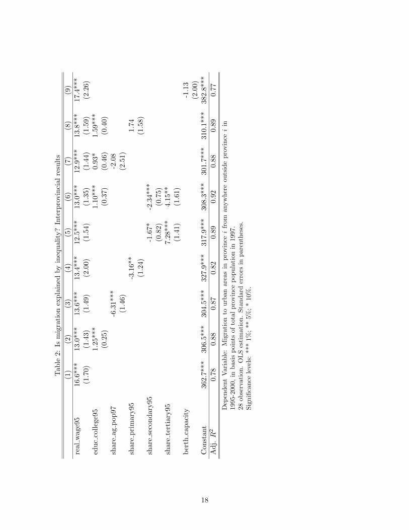
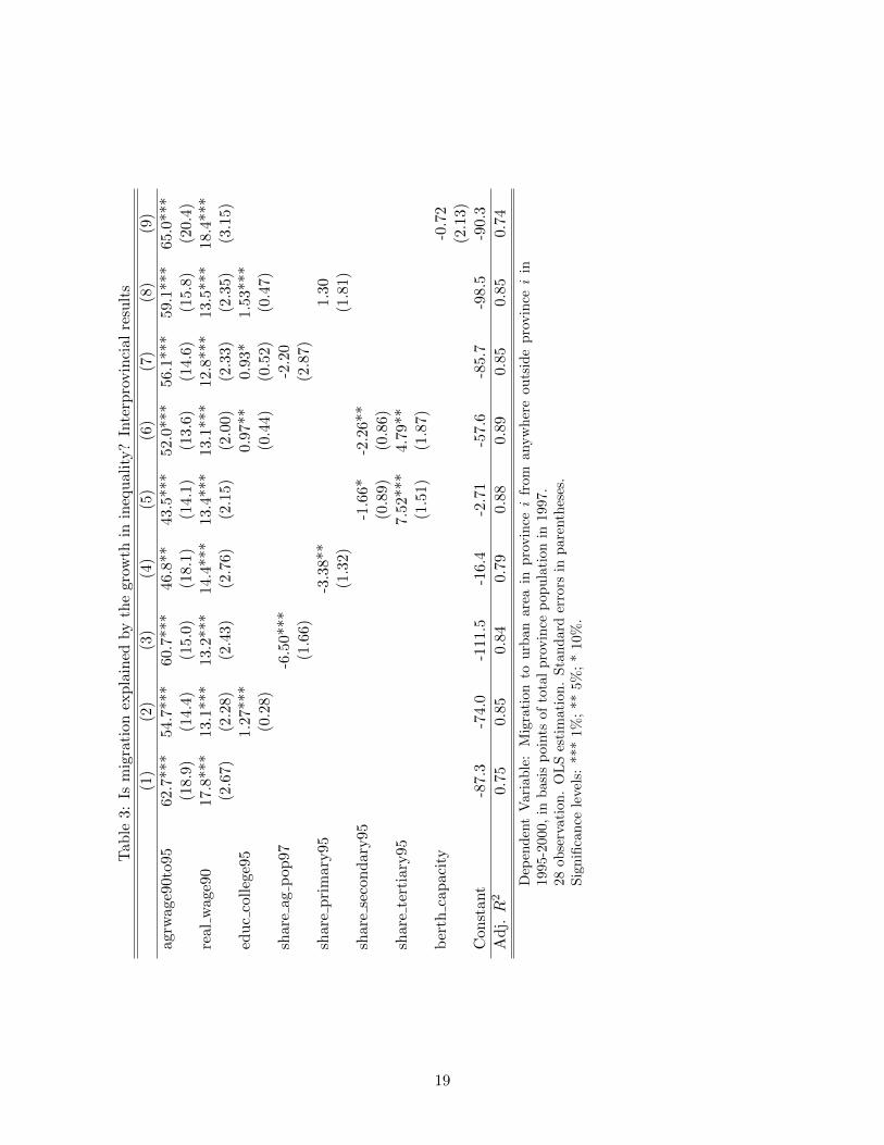
Before addressing the question of whether cross-province migration offsets some of the wage dif-

ferences, we have to establish that cross-province migration is driven at least in part by wage

differences. To this end, we test whether cross-province migration into urban areas between 1995

and 2000 is correlated with differences in real wages across provinces in 1995 (Table 2) and, al-

ternatively, with differences in real wages in 1990 and differences in the growth rate of real wages

between 1990 and 1995 (Table 3). In such a setup, migration does not affect wage differences.13 We

find that both the level and the growth rate of real wages have positive effects on migration into

urban areas of a given province from other provinces.14 These results hold even when we control

for the offsetting factors that we found to be important in the first part of our analysis.

Coefficients on offsetting factors have expected signs — higher education and larger share of

tertiary industries attract more migrants, while a higher share of agricultural population and higher

share of primary industries lower the inflow of migrants. Interestingly, the share of secondary

industries, while associated with higher wages (see Table 1), has a negative effect on migration,

while tertiary industries seem to attract migrants. Berth capacity does not enter significantly in

these regressions.

Having established that migration is indeed driven by wage differences, we now turn to the main

question of interest — Does migration offset any of the wage differences? To this end, we estimate

the effect of cross-province migration into urban areas between 1995 and 2000 on real wages in

2001, while controlling for our offsetting factors in 2001. The results are reported in Table 4.15

In column (1) we see that, far from offsetting wage differences, higher migration is associated

with higher real wages. This effect is spurious, however. Because real wage differences across

provinces are highly persistent over time, migration in 1995-2000 may be endogenous even with

respect to 2001 real wages. To rule out this possibility, in column (2) we add the real wage in 1995

as an additional control variable. Once this control is included, migration no longer has a positive

13An important caveat is that, because of the cross-section nature of the migration data, we are down to 28observations and a cross-province regression.

14For comparison, Tables A.5 and A.6 provide the same analysis for rural-to-urban migration within provinces.15For comparison, results of similar tests for rural-to-urban migration within provinces are reported in Table A.7.

12

effect on real wages. In fact, we find a negative effect in some specifications, which would indicate

that there is some equalizing effect of migration, although this negative effect is never statistically

significant and the reduction in the variance of the residual is minimal to nil (comparing column

(2) with column (11)). We conclude, therefore, that the cross-province migration that occurred

between 1995 and 2000 did not produce any equalizing effects.

5 Conclusion

Provincial statistics show that regional inequality in China has been persistent and even growing

in the past two decades. We find that the main sources of this growth were structural and long-

term factors such as labor quality, industrial composition, and geographical location. We find

that interprovincial transfers did not offset wage inequality during our sample period, nor did

interprovince migration. These findings suggest that regional income inequality in China is not

likely to go away in the near future.

While we believe that fully removing barriers to labor mobility will help reduce cross-province

wage inequality, we are aware that urban infrastructure is unable to accommodate large inflows of

new migrants. We therefore view the message of this paper as more positive than normative —

given the gradual nature of structural changes and urban infrastructure development, we should

expect regional inequality in China to persist for quite some time.

A policy implication of this observation is that social tensions that arise from such inequality

may need to be addressed in the short run through redistribution. According to our analysis of the

measures we considered, such redistribution has not been present during our sample period . The

Chinese government, however, recognizes inequality as an important problem, which is reflected in

its most recent five–year plan.

13

References

Bound, J., and H. J. Holzer (2000): “Demand Shifts, Population Adjustments, and Labor

Market Outcomes during the 1980s,” Journal of Labor Economics, 18(1), 20–54.

Candelaria, C., M. Daly, and G. Hale (2009): “Interprovincial Inequality in China,” FRBSF

Economic Letter, 2009-13.

Chan, K. W., and Y. Hu (2003): “Urbanization in China in the 1990s: New Definition, Different

Series, and Revised Trends,” The China Review, 3(2), 49–71.

Cremer, H., and P. Pestieau (2007): “Factor Mobility and Redistribution,” in Handbook of

Regional and Urban Economics, vol. 4, pp. 2529–2560. Elsevier B.V.

Fan, C. C. (2005): “Interprovincial Migration, Population Redistribution, and Regional Devel-

opment in China: 1990 and 2000 Census Comparisons,” The Professional Geographer, 57(2),

295–311.

Fujita, M., and D. Hu (2001): “Regional disparity in China 19851994: The effects of globalization

and economic liberalization,” The Annals of Regional Science, 35(1), 3–37.

Huber, P. (2006): “Regional Labor Market Developments in Transition,” World Bank Policy

Research Working Paper No. 3896.

Jian, T., J. D. Sachs, and A. M. Warner (1996): “Trends in Regional Inequality in China,”

China Economic Review, 7(1), 1–21.

Kanbur, R., and X. Zhang (1999): “Which Regional Inequality? The Evolution of Rural-Urban

and Inland-Coastal Inequality in China from 1983 to 1995,” Journal of Comparative Economics,

27(4).

(2005): “Fifty Years of Regional Inequality in China: A Journey through Central Planning,

Reform, and Openness,” Review of Development Economics, 9(1), 87–106.

Lavely, W. (2001): “First Impressions from the 2000 Census of China,” Population and Develop-

ment Review, 27(4), 755–769.

14

Magrini, S. (2007): “Regional (di)convergence,” in Handbook of Regional and Urban Economics,

vol. 4, pp. 2741–2796. Elsevier B.V.

Meng, X., R. Gregory, and Y. Want (2005): “Poverty, Inequality, and Growth in Urban

China, 1986-2000,” Journal of Comparative Economics, 33(4), 710–729.

Rice, P., and A. Venables (2003): “Equilibrium Regional Disparities: Theory and British

Evidence,” Regional Studies.

Wan, G., M. Lu, and Z. Chen (2007): “Globalization and Regional Income Inequality: Empirical

Evidence from within China,” The Review of Income and Wealth, 53(1), 35–59.

Wang, F.-L. (2005): “China’s Household Registration (Hukou) System: Discrim-

ination and Reform,” Discussion paper, Congressional Statement, available at

http://www.cecc.gov/pages/roundtables/090205/Wang.php.

Whalley, J., and S. Zhang (2004): “Inequality Change in China and (Hukou) Labour Mobility

Restrictions,” NBER Working Paper 10683.

Yao, S., and Z. Zhang (2001): “On Regional Inequality and Diverging Clubs: A Case Study of

Contemporary China,” Journal of Comparative Economics, 29(3), 466–484.

15

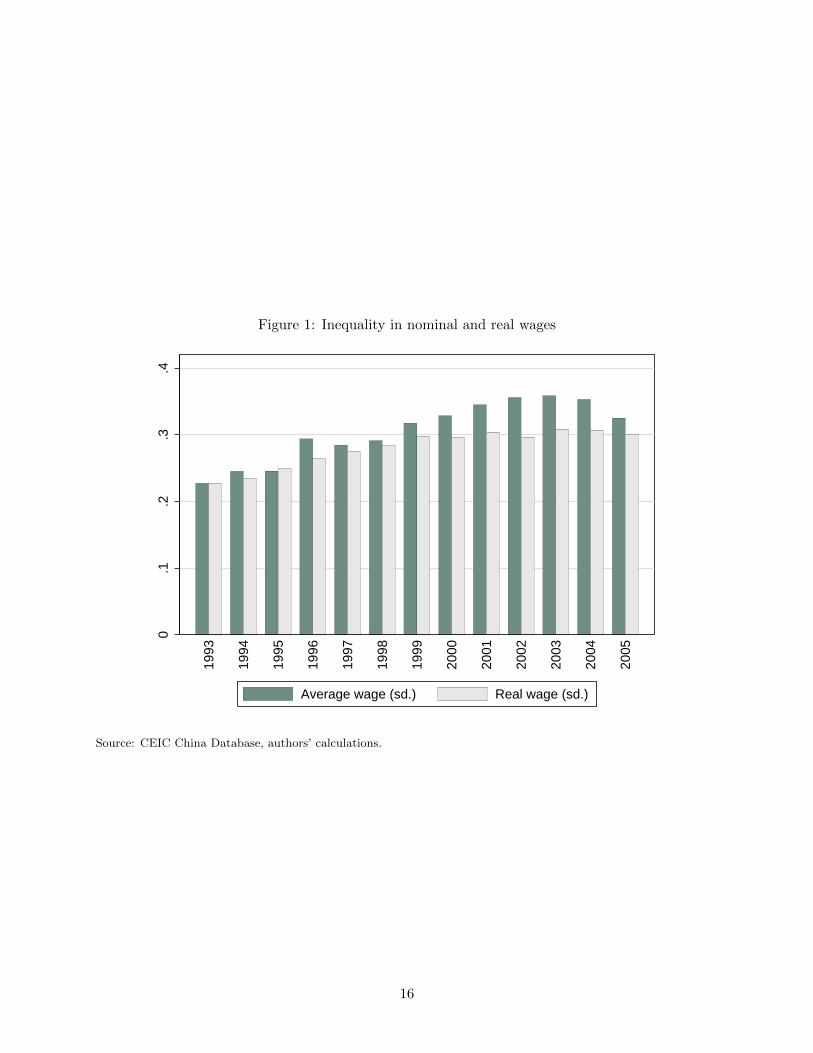
Figure 1: Inequality in nominal and real wages

0.1

.2.3

.4

1993

1994

1995

1996

1997

1998

1999

2000

2001

2002

2003

2004

2005

Average wage (sd.) Real wage (sd.)

Source: CEIC China Database, authors’ calculations.

16

Tab

le1:

Are

offse

ttin

gfa

ctor

san

exp

lan

atio

nfo

rw

age

ineq

ual

ity?

(1)

(2)

(3)

(4)

(5)

(6)

(7)

(8)

(9)

edu

cco

lleg

e0.

12**

*(0

.009

6)ed

uc

spen

din

g0.

36**

*(0

.015

)sh

are

pri

mar

y-0

.52*

**(0

.025

)sh

are

seco

nd

ary

0.35

***

0.25

***

(0.0

20)

(0.0

25)

shar

ete

rtia

ry0.

49**

*0.

25**

*(0

.032

)(0

.037

)sh

are

agp

op-0

.67*

**(0

.051

)b

erth

cap

acit

y0.6

5***

(0.0

39)

govt

tran

sfer

0.0

88***

(0.0

26)

Con

stan

t-8

.44*

**-1

0.9*

**-7

.12*

**-5

.33*

**-8

.68*

**-6

.90*

**-1

0.2*

**-1

4.5

***

-8.3

4***

Ad

j.R

20.

280.

710.

530.

440.

370.

500.

380.4

10.0

45

Ob

serv

atio

ns

392

224

392

392

392

392

280

392

224

1st

dat

aye

ar19

9319

9919

9319

9319

9319

9319

971993

1999

S.D

.of

resi

dual

19.8

10.8

11.0

17.2

16.6

13.4

15.3

18.3

24.4

Dep

end

ent

vari

able

:A

vera

ge

real

wage,

inp

erce

nta

ge

dev

iati

on

from

Ch

ina

mea

n.

Nu

mb

erof

pro

vin

ces:

28;

S.D

.of

real

wage

(2006):

23.7

;la

std

ata

yea

r:2006.

OL

Ses

tim

atio

n.

Sta

nd

ard

erro

rsin

pare

nth

eses

.S

ign

ifica

nce

level

s:**

*1%

;**

5%

;*

10%

.

17

Tab

le2:

Ism

igra

tion

exp

lain

edby

ineq

ual

ity?

Inte

rpro

vin

cial

resu

lts

(1)

(2)

(3)

(4)

(5)

(6)

(7)

(8)

(9)

real

wag

e95

16.6

***

13.0

***

13.6

***

13.4

***

12.5

***

13.0

***

12.9

***

13.8

***

17.4

***

(1.7

0)(1

.43)

(1.4

9)(2

.00)

(1.5

4)(1

.35)

(1.4

4)

(1.5

9)

(2.2

6)

edu

cco

lleg

e95

1.25

***

1.10

***

0.93

*1.5

9***

(0.2

5)(0

.37)

(0.4

6)

(0.4

0)

shar

eag

pop

97-6

.31*

**-2

.08

(1.4

6)(2

.51)

shar

ep

rim

ary95

-3.1

6**

1.7

4(1

.24)

(1.5

8)

shar

ese

con

dar

y95

-1.6

7*-2

.34*

**(0

.82)

(0.7

5)sh

are

tert

iary

957.

28**

*4.

15**

(1.4

1)(1

.61)

ber

thca

pac

ity

-1.1

3(2

.00)

Con

stan

t36

2.7*

**30

6.5*

**30

4.5*

**32

7.9*

**31

7.9*

**30

8.3*

**30

1.7*

**

310.1

***

382.8

***

Ad

j.R

20.

780.

880.

870.

820.

890.

920.

880.8

90.7

7

Dep

end

ent

Var

iab

le:

Mig

rati

on

tou

rban

are

as

inp

rovin

cei

from

anyw

her

eou

tsid

ep

rovin

cei

in19

95-2

000,

inb

asis

poi

nts

of

tota

lp

rovin

cep

op

ula

tion

in1997.

28ob

serv

atio

n.

OL

Ses

tim

ati

on.

Sta

nd

ard

erro

rsin

pare

nth

eses

.S

ign

ifica

nce

level

s:**

*1%

;**

5%

;*

10%

.

18

Tab

le3:

Ism

igra

tion

exp

lain

edby

the

grow

thin

ineq

ual

ity?

Inte

rpro

vin

cial

resu

lts

(1)

(2)

(3)

(4)

(5)

(6)

(7)

(8)

(9)

agrw

age9

0to9

562

.7**

*54

.7**

*60

.7**

*46

.8**

43.5

***

52.0

***

56.1

***

59.1

***

65.0

***

(18.

9)(1

4.4)

(15.

0)(1

8.1)

(14.

1)(1

3.6)

(14.

6)(1

5.8

)(2

0.4

)re

alw

age9

017

.8**

*13

.1**

*13

.2**

*14

.4**

*13

.4**

*13

.1**

*12

.8**

*13.5

***

18.4

***

(2.6

7)(2

.28)

(2.4

3)(2

.76)

(2.1

5)(2

.00)

(2.3

3)(2

.35)

(3.1

5)

edu

cco

lleg

e95

1.27

***

0.97

**0.

93*

1.5

3***

(0.2

8)(0

.44)

(0.5

2)(0

.47)

shar

eag

pop

97-6

.50*

**-2

.20

(1.6

6)(2

.87)

shar

ep

rim

ary95

-3.3

8**

1.3

0(1

.32)

(1.8

1)

shar

ese

con

dar

y95

-1.6

6*-2

.26*

*(0

.89)

(0.8

6)sh

are

tert

iary

957.

52**

*4.

79**

(1.5

1)(1

.87)

ber

thca

pac

ity

-0.7

2(2

.13)

Con

stan

t-8

7.3

-74.

0-1

11.5

-16.

4-2

.71

-57.

6-8

5.7

-98.5

-90.3

Ad

j.R

20.

750.

850.

840.

790.

880.

890.

850.8

50.7

4

Dep

end

ent

Var

iab

le:

Mig

rati

on

tou

rban

are

ain

pro

vin

cei

from

anyw

her

eou

tsid

epro

vin

cei

in19

95-2

000,

inb

asis

poi

nts

of

tota

lp

rovin

cep

op

ula

tion

in1997.

28ob

serv

atio

n.

OL

Ses

tim

ati

on.

Sta

nd

ard

erro

rsin

pare

nth

eses

.S

ign

ifica

nce

level

s:**

*1%

;**

5%

;*

10%

.

19

Tab

le4:

Does

mig

rati

onre

du

cein

equ

alit

y?

Inte

rpro

vin

cial

resu

lts

(1)

(2)

(3)

(4)

(5)

(6)

(7)

(8)

(9)

(10)

(11)

xp

mig

rati

on0.

056*

**0.

000

-0.0

097

-0.0

17-0

.008

5-0

.001

5-0

.010

-0.0

029

-0.0

12

0.0

0050

(0.0

071)

(0.0

091)

(0.0

13)

(0.0

10)

(0.0

097)

(0.0

086)

(0.0

12)

(0.0

13)

(0.0

12)

(0.0

093)

real

wag

e95

1.19

***

1.28

***

1.16

***

1.17

***

1.06

***

1.27

***

1.08

***

1.2

9***

1.1

5***

1.1

9***

(0.1

7)(0

.19)

(0.1

5)(0

.16)

(0.1

7)(0

.18)

(0.2

2)

(0.1

8)

(0.1

9)

(0.0

77)

edu

cco

lleg

e01

0.02

9(0

.027

)ed

uc

spen

din

g01

0.14

**(0

.052

)sh

are

pri

mar

y01

-0.1

5*(0

.077

)sh

are

seco

nd

ary01

0.11

**0.

10(0

.053

)(0

.066

)sh

are

tert

iary

010.

120.

016

(0.0

93)

(0.1

1)

shar

eag

pop

01-0

.17

(0.1

1)

ber

th0.0

42

(0.0

93)

Con

stan

t-2

0.0*

**1.

934.

444.

443.

922.

404.

292.

714.5

31.0

11.9

4

Ad

j.R

20.

700.

890.

890.

920.

900.

910.

900.

900.9

00.8

90.9

0S

.D.

ofre

sidu

al13

.67.

917.

726.

907.

357.

287.

677.

287.5

47.8

87.9

1

Dep

end

ent

vari

able

:A

vera

ge

real

wage,

inp

erce

nta

ge

dev

iati

on

from

Ch

ina

mea

nN

um

ber

ofp

rovin

ces:

28;

S.D

.of

real

wage:

25.2

(2001);

OL

Ses

tim

atio

n.

Sta

nd

ard

erro

rsin

pare

nth

eses

.S

ign

ifica

nce

leve

ls:

***

1%

;**

5%

;*

10%

.

20

A Appendix

Table A.1: Variable Definitions

nominal wage Average annual wage in yuan per person for staff and workers in enterprises,institutions, and government agencies, which reflects the general level of wage income.

cpi Consumer price index; 1988 = 100.

real wage Average annual wage in yuan per person for staff and workers in enterprises, institu-tions, and government agencies deflated by the consumer price index (1988 = 100).

educ college Number of college graduates of regular institutions of higher learning scaled bypopulation.

educ spending Expenditure of provincial government on education scaled by population.

share primary Share of employees involved in the production of raw goods (primary sector).

share secondary Share of employees involved in the manufacture of goods (secondary sector).

share tertiary Share of employees in the services sector (tertiary sector).

share ag pop Share of agricultural population.

berth capacity Number of berths in major coastal ports (10,000 ton class, end of year 2000).

govt transfer National government subsidy to provincial government per capita.

xp migration Number of migrants moving into an urban area of a province from an urban orrural area in another province. This variable is scaled by population in 1997 in the destinationprovince (in basis points).

ru migration Number of migrants moving into an urban area of a given province from a ruralarea in that province. This variable is scaled by the population in 1997 in the province (inbasis points).

21

Table A.2: Summary Statistics

Name 1st year data Mean (level) Std. Dev.(level) Mean (PD) Std. Dev (PD)

nominal wage 1993 10491.9 6483.7 1.95 30.3cpi 1993 249.7 37.1 – –real wage 1993 3950.4 2005.6 -5.93 22.7educ college 1993 0.001 .001 18.5 99.9educ spending 1999 77.1 52.9 12.5 56.0share primary 1993 0.49 0.16 -0.67 32.1share secondary 1993 0.22 0.10 -4.1 43.8share tertiary 1993 0.29 0.08 4.7 28.1share ag pop 1997 0.68 0.16 -5.3 22.0berth capacity 1993 12.8 22.2 – –govt transfer 1999 303.6 177.5 21.9 60.3xp migration 1993 0.26 0.36 – –ru migration 1993 0.24 0.10 – –

See Table A.1. for variable definitions.PD is percent deviation from country average in each year.

22

Table A.3: Migration Statistics: Cross-Province and Intraprovince

Cross-Province IntraprovinceIn–migration to urban area In–migration to urban area from rural area

Gross number Share province pop Gross Number Share province pop(thousands) (basis points) (thousands) (basis points)

Anhui 174 .028 1143 .19Beijing 1592 1.3 227 .18Chongqing/Sichuan 448 .039 3031 .26Fujian 905 .28 1413 .43Gansu 182 .073 468 .19Guangdong 8534 1.2 3863 .55Guangxi 236 .051 1116 .24Guizhou 202 .056 681 .19Hainan 183 .25 191 .26Hebei 497 .076 1415 .22Heilongjiang 238 .063 613 .16Henan 326 .035 1576 .17Hunan 273 .042 1429 .22Inner Mongolia 228 .098 797 .34Jiangsu 1265 .18 2168 .3Jiangxi 163 .039 922 .22Jilin 206 .079 413 .16Liaoning 600 .14 742 .18Ningxia 76 .14 141 .27Qinghai 70 .14 90 .18Shaanxi 366 .1 714 .2Shandong 667 .076 2860 .33Shanghai 1947 1.3 344 .24Shanxi 225 .072 734 .23Tianjin 442 .46 148 .16Xinjiang 551 .32 324 .19Yunnan 627 .15 1042 .25Zhejiang 1892 .43 2236 .5

23

Tab

leA

.4:

Cor

rela

tion

mat

rix

for

offse

ttin

gfa

ctor

s.

Nob

s.=

224

edu

cco

lleg

eed

uc

spen

din

gsh

are

pri

mar

ysh

are

seco

nd

ary

shar

ete

rtia

rysh

are

ag

pop

ber

thca

paci

ty

edu

cco

lleg

e1.

000.

81-0

.82

0.63

0.85

-0.8

10.3

5ed

uc

spen

din

g0.

811.

00-0

.86

0.71

0.80

-0.8

60.5

6sh

are

pri

mar

y-0

.82

-0.8

61.

00-0

.88

-0.8

60.8

3-0

.59

shar

ese

con

dar

y0.

630.

71-0

.88

1.00

0.53

-0.6

20.6

7sh

are

tert

iary

0.85

0.80

-0.8

60.

531.

00-0

.84

0.3

5sh

are

agp

op-0

.81

-0.8

60.

83-0

.62

-0.8

41.0

0-0

.53

ber

thca

pac

ity

0.35

0.56

-0.5

90.

670.

35-0

.53

1.0

0

24

Tab

leA

.5:

Ism

igra

tion

exp

lain

edby

ineq

ual

ity?

Intr

apro

vin

cial

resu

lts

(1)

(2)

(3)

(4)

(5)

(6)

(7)

(8)

(9)

real

wag

e95

2.61

***

4.30

***

4.04

***

4.25

***

4.33

***

3.96

***

4.34

***

4.0

7***

2.8

3**

(0.8

3)(0

.72)

(0.7

5)(0

.97)

(0.9

9)(0

.84)

(0.7

3)

(0.8

2)

(1.1

1)

edu

cco

lleg

e95

-0.5

8***

-0.7

5***

-0.4

4*

-0.6

9***

(0.1

3)(0

.23)

(0.2

3)

(0.2

1)

shar

eag

pop

972.

94**

*0.

92(0

.74)

(1.2

8)

shar

ep

rim

ary95

1.60

**-0

.51

(0.6

0)(0

.81)

shar

ese

con

dar

y95

-0.4

60.

0052

(0.5

3)(0

.46)

shar

ete

rtia

ry95

-1.2

30.

93(0

.90)

(1.0

0)b

erth

cap

acit

y-0

.30

(0.9

8)

Con

stan

t26

6.6*

**29

2.9*

**29

3.7*

**28

4.2*

**28

5.0*

**29

1.6*

**29

5.0*

**

291.8

***

271.9

***

(17.

2)(1

4.1)

(15.

3)(1

6.8)

(17.

1)(1

4.5)

(14.

6)

(14.4

)(2

4.7

)A

dj.

R2

0.25

0.58

0.52

0.39

0.37

0.56

0.57

0.5

70.2

2N

obs.

2828

2828

2828

2828

28

Dep

end

ent

Var

iab

le:

Ru

ral

toU

rban

Intr

am

igra

tion

Nob

s.:

28O

LS

esti

mat

ion

.S

tan

dard

erro

rsin

pare

nth

eses

.S

ign

ifica

nce

level

s:**

*1%

;**

5%

;*

10%

.

25

Tab

leA

.6:

Ism

igra

tion

exp

lain

edby

the

grow

thin

ineq

ual

ity?

Intr

apro

vin

cial

resu

lts

(1)

(2)

(3)

(4)

(5)

(6)

(7)

(8)

(9)

agrw

age9

0to9

526

.7**

*30

.0**

*27

.4**

*33

.7**

*33

.9**

*28

.0**

*29

.8**

*28.9

***

27.0

***

(8.2

5)(6

.46)

(6.9

3)(7

.89)

(8.0

4)(7

.32)

(6.6

4)(7

.14)

(8.9

3)

real

wag

e90

0.76

2.75

**2.

59**

2.30

*2.

36*

2.61

**2.

81**

2.6

6**

0.8

5(1

.17)

(1.0

2)(1

.12)

(1.2

0)(1

.23)

(1.0

8)(1

.06)

(1.0

6)

(1.3

8)

edu

cco

lleg

e95

-0.5

3***

-0.6

7***

-0.4

7*-0

.60***

(0.1

3)(0

.24)

(0.2

4)(0

.21)

shar

eag

pop

972.

58**

*0.

40(0

.76)

(1.3

0)sh

are

pri

mar

y95

1.51

**-0

.34

(0.5

7)(0

.82)

shar

ese

con

dar

y95

-0.4

6-0

.051

(0.5

1)(0

.47)

shar

ete

rtia

ry95

-1.0

90.

81(0

.87)

(1.0

1)b

erth

cap

acit

y-0

.12

(0.9

3)

Con

stan

t11

1.8*

*10

6.2*

**12

1.5*

**80

.3*

79.4

*11

7.6*

**10

8.4*

**

112.7

***

111.3

**

(44.

9)(3

4.9)

(37.

8)(4

2.1)

(42.

9)(3

9.8)

(36.

2)(3

8.7

)(4

5.9

)A

dj.

R2

0.31

0.58

0.51

0.44

0.42

0.56

0.57

0.5

70.2

8N

obs.

2828

2828

2828

2828

28

Dep

.V

ar.:

Ru

ral

toU

rban

Intr

am

igra

tion

Nob

s.:

28O

LS

esti

mat

ion

.S

tan

dard

erro

rsin

pare

nth

eses

.S

ign

ifica

nce

level

s:**

*1%

;**

5%

;*

10%

.

26

Tab

leA

.7:

Does

mig

rati

onre

du

cein

equ

alit

y?

Intr

apro

vin

cial

resu

lts

(1)

(2)

(3)

(4)

(5)

(6)

(7)

(8)

(9)

(10)

rum

igra

tion

0.13

***

0.01

30.

036

0.04

5**

0.03

00.

022

0.02

60.0

26

0.0

41*

0.0

13

(0.0

42)

(0.0

18)

(0.0

23)

(0.0

19)

(0.0

19)

(0.0

17)

(0.0

20)

(0.0

19)

(0.0

22)

(0.0

19)

real

wag

e95

1.15

***

1.00

***

0.75

***

0.94

***

0.95

***

1.04

***

0.93***

0.9

7***

1.1

2***

(0.0

92)

(0.1

3)(0

.15)

(0.1

3)(0

.12)

(0.1

2)(0

.13)

(0.1

2)

(0.1

2)

edu

cco

lleg

e01

0.03

9(0

.024

)ed

uc

spen

din

g01

0.15

***

(0.0

46)

shar

ep

rim

ary01

-0.1

7**

(0.0

73)

shar

ese

con

dar

y01

0.12

**0.1

1*

(0.0

52)

(0.0

59)

shar

ete

rtia

ry01

0.10

0.041

(0.0

75)

(0.0

79)

shar

eag

pop

01-0

.21**

(0.0

99)

ber

th0.0

45

(0.0

92)

Con

stan

t-3

9.1*

**-1

.46

-9.1

0-1

4.0*

*-7

.17

-4.0

0-6

.21

-5.6

2-1

1.1

-2.4

2

Ad

j.R

20.

260.

900.

900.

920.

910.

910.

900.9

10.9

10.8

9S

.D.

ofre

sidu

al21

.37.

847.

446.

557.

107.

067.

547.0

27.1

77.8

0

Dep

end

ent

vari

able

:R

eal

Wage

PD

.N

um

ber

ofp

rovin

ces:

28;

S.D

.of

real

wage:

25.2

(2001);

OL

Ses

tim

atio

n.

Sta

nd

ard

erro

rsin

pare

nth

eses

.S

ign

ifica

nce

level

s:**

*1%

;**

5%

;*

10%

.

27