BEYOND LINEAR ALGEBRA

Bernd SturmfelsUniversity of California at Berkeley

Renaissance Technologies Colloquium, March 25, 2014

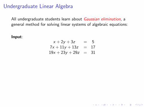
Undergraduate Linear Algebra

All undergraduate students learn about Gaussian elimination, ageneral method for solving linear systems of algebraic equations:

Input:x + 2y + 3z = 5

7x + 11y + 13z = 1719x + 23y + 29z = 31

Output:x = −35/18y = 2/9z = 13/6

Solving very large linear systems is central to applied mathematics.

Undergraduate Linear Algebra

All undergraduate students learn about Gaussian elimination, ageneral method for solving linear systems of algebraic equations:

Input:x + 2y + 3z = 5

7x + 11y + 13z = 1719x + 23y + 29z = 31

Output:x = −35/18y = 2/9z = 13/6

Solving very large linear systems is central to applied mathematics.

Undergraduate Non-Linear Algebra

Lucky undergraduate students also learn about Grobner bases,a general method for non-linear systems of algebraic equations:

Input: x2 + y 2 + z2 = 2x3 + y 3 + z3 = 3x4 + y 4 + z4 = 4

Output:

3z12−12z10−12z9+12z8+72z7−66z6−12z4+12z3−1 = 0

4y 2 + (36z11+54z10−69z9−252z8−216z7+573z6+72z5

−12z4−99z3+10z+3) · y + 36z11+48z10−72z9

−234z8−192z7+564z6−48z5+96z4−96z3+10z2+8 = 0

4x + 4y + 36z11+54z10−69z9−252z8−216z7

+573z6+72z5−12z4−99z3+10z+3 = 0

Non-linear equations can be intimidating, but ....

Undergraduate Non-Linear Algebra

Lucky undergraduate students also learn about Grobner bases,a general method for non-linear systems of algebraic equations:

Input: x2 + y 2 + z2 = 2x3 + y 3 + z3 = 3x4 + y 4 + z4 = 4

Output:

3z12−12z10−12z9+12z8+72z7−66z6−12z4+12z3−1 = 0

4y 2 + (36z11+54z10−69z9−252z8−216z7+573z6+72z5

−12z4−99z3+10z+3) · y + 36z11+48z10−72z9

−234z8−192z7+564z6−48z5+96z4−96z3+10z2+8 = 0

4x + 4y + 36z11+54z10−69z9−252z8−216z7

+573z6+72z5−12z4−99z3+10z+3 = 0

Non-linear equations can be intimidating, but ....

Truth and BeautyMany models in the sciences and engineering are characterized bypolynomial equations. Such a set is an algebraic variety X ⊂ Rn.

This Lecture

What I shall speak about:

I Tensor Decomposition

I Polynomial Optimization

I Algebraic Statistics

Linear algebra is the foundation of scientific computing and its numerous applications. Yet, the world is non-linear.

We argue that it pays off to work with models described by non-linear polynomials, while still taking advantage of

the power of numerical linear algebra. This leads us to applied algebraic geometry. We present a glimpse of this

area, by discussing recent advances in tensor decomposition, polynomial optimization, and algebraic statistics.

Topic 1: TENSOR DECOMPOSITIONA tensor is an n-dimensional array of numbers (xi1i2···in).For n = 1 this is a vector, and for n = 2 this is a matrix.

The vector space of 3×3×3-tensors has dimension 27:

A tensor has rank one if it is the outer product of n vectors.

3×3×3-tensors of rank 1 have the form

xijk = aibjck for 1 ≤ i , j , k ≤ 3.

Book: JM Landsberg: Tensors: Geometry and Applications, 2012.

Does Watching Soccer Cause Hair Loss?296 subjects aged 40 to 50 were asked about their hair length andhow many hours per week they watch soccer on TV. The data aresummarized in a 3× 3 matrix. Is it close to having rank 1?

U =

lots of hair medium hair little hair

≤ 2 hrs 51 45 332–6 hrs 28 30 29≥ 6 hrs 15 27 38

Is there a correlation between watching soccer and hair loss?

Not really. There is a hidden random variable, namely gender. Thetable is the sum of a table for 126 males and one for 170 females:

U =

3 9 154 12 207 21 35

+

48 36 1824 18 98 6 3

.

Both matrices have rank 1, hence U has rank 2. We cannot reject

H0 : Soccer on TV and Hair Growth are Independent Given Gender.

Does Watching Soccer Cause Hair Loss?296 subjects aged 40 to 50 were asked about their hair length andhow many hours per week they watch soccer on TV. The data aresummarized in a 3× 3 matrix. Is it close to having rank 1?

U =

lots of hair medium hair little hair

≤ 2 hrs 51 45 332–6 hrs 28 30 29≥ 6 hrs 15 27 38

Is there a correlation between watching soccer and hair loss?

Not really. There is a hidden random variable, namely gender. Thetable is the sum of a table for 126 males and one for 170 females:

U =

3 9 154 12 207 21 35

+

48 36 1824 18 98 6 3

.

Both matrices have rank 1, hence U has rank 2. We cannot reject

H0 : Soccer on TV and Hair Growth are Independent Given Gender.

Decomposition and RankThe soccer-hair example illustrates the importance ofdecomposing a matrix as a sum of rank 1 matrices.

Tensor decomposition:I Express a given tensor as a sum of rank one tensors.I Use as few summands as possible.

A tensor has rank r if it is the sum of r tensors of rank one (not fewer).

A nonnegative tensor has nonnegative rank r ifit is the sum of r nonnegative tensors of rank one (but not fewer).

Henri Poincare said ...

Mathematics is the art of giving the same name to different things.

Aren’t the following eight things “different”?

I the set of 4×4×4 tensors of rank ≤ 4,

I xijkl = a1ib1jc1kd1l +a2ib2jc2kd2l +a3ib3jc3kd3l +a4ib4jc4kd4l .

I the fourth mixture model for 3 independent random variables,

I the naive Bayes model with four classes,

I the conditional independence model [ X1 ⊥⊥ X2 ⊥⊥ X3 |Y ],

I the fourth secant variety of the Segre variety P3 × P3 × P3,

I the general Markov model for the phylogenetic tree K1,3,

I superpositions of four pure states in quantum systems.

Allman’s Salmon Problem: What are equations describing this set?

Solved recently by Friedland-Gross and Bates-Oeding.

Rank Two

A tensor can be written as a matrix by aggregating indices.

Such a matrix is a flattening of the tensor.

Example: the flattenings of a 2×3×5×7-tensor are matrices offormats 2×105, 3×70, 5×42, 7×30, 6×35, 10×21 and 14×15.

Theorem (Landsberg-Manivel, Raicu)

A tensor (of any format) has rank ≤ 2 if and only ifall its matrix flattenings have rank ≤ 2.

Fine print: this is true up to closure, over the complex numbers.

Theorem (Allman-Rhodes-St-Zwiernik)

A nonnegative tensor (of any format) has nonnegative rank ≤ 2if and only if it has rank 2 and it is supermodular,

i.e. it satisfies certain quadratic inequalities like x111x222 ≥ x122x211.

Higher Rank

... is more complicated:

Theorem (Strassen 1983)

A 3× 3× 3-tensor has rank ≤ 4 if and only ifa certain explicit polynomial of degree 9 vanishes.

... but still finite:

Theorem (Draisma-Kuttler 2014)

For any given r there exists an integer D(r) such that a tensor hasrank ≤ r if and only if certain polynomials of degree ≤ D(r) vanish.

Topic 2: POLYNOMIAL OPTIMIZATION

A spectrahedron is the intersection of the cone ofpositive semidefinite matrices with a linear space.

Semidefinite programming is the problem of minimizinga linear function over a spectrahedron. Can be done efficiently.

For diagonal matrices: polyhedron and linear programming.

Duality

Sums of Squares

Let f (x1, . . . , xm) be a polynomial of even degree 2d.Goal: compute the global minimum x∗ of f (x) on Rm.

This optimization problem is hard. It is equivalent to

Maximize λ such that f (x)− λ is non-negative on Rm.

The following relaxation gives a lower bound:

Maximize λ such that f (x)− λ is a sum of squares of polynomials.

This is much easier. It is a semidefinite program.

The optimal value of the SDP often agrees with the globalminimum, and optimal point x∗ can be recovered [Parrilo-St 2003].

Book: G. Blekherman, P. Parrilo, R. Thomas:Semidefinite Optimization and Convex Algebraic Geometry, 2013

Sums of Squares

Let f (x1, . . . , xm) be a polynomial of even degree 2d.Goal: compute the global minimum x∗ of f (x) on Rm.

This optimization problem is hard. It is equivalent to

Maximize λ such that f (x)− λ is non-negative on Rm.

The following relaxation gives a lower bound:

Maximize λ such that f (x)− λ is a sum of squares of polynomials.

This is much easier. It is a semidefinite program.

The optimal value of the SDP often agrees with the globalminimum, and optimal point x∗ can be recovered [Parrilo-St 2003].

Book: G. Blekherman, P. Parrilo, R. Thomas:Semidefinite Optimization and Convex Algebraic Geometry, 2013

SOS ExampleLet m = 1, d = 2 and f (x) = 3x4 + 4x3 − 12x2. Then

f (x)− λ =(x2 x 1

) 3 2 µ− 62 −2µ 0

µ− 6 0 −λ

x2

x1

Maximize λ over (λ, µ) s.t. the 3×3-matrix is positive semidefinite.

The solution to this semidefinite program is

(λ∗, µ∗) = (−32,−2).

Cholesky factorization reveals the sum of squares representation

f (x)− λ∗ =((√

3 x − 4√3

) · (x + 2))2

+8

3

(x + 2

)2.

We conclude that the global minimum is x∗ = −2.

This approach works for a wide range of optimization problems.

SOS ExampleLet m = 1, d = 2 and f (x) = 3x4 + 4x3 − 12x2. Then

f (x)− λ =(x2 x 1

) 3 2 µ− 62 −2µ 0

µ− 6 0 −λ

x2

x1

Maximize λ over (λ, µ) s.t. the 3×3-matrix is positive semidefinite.

The solution to this semidefinite program is

(λ∗, µ∗) = (−32,−2).

Cholesky factorization reveals the sum of squares representation

f (x)− λ∗ =((√

3 x − 4√3

) · (x + 2))2

+8

3

(x + 2

)2.

We conclude that the global minimum is x∗ = −2.

This approach works for a wide range of optimization problems.

Distance MinimizationFor any variety X , we study the following optimization problem:

for any data point u ∈ Rn, find x ∈ X that minimizesthe Euclidean distance function x 7→

∑ni=1(ui − xi )

2.

[Draisma-Horobet-Ottaviani-St-Thomas:

The Euclidean Distance Degree of an Algebraic Variety, 2013]

Topic 3: ALGEBRAIC STATISTICSWhat is a “statistical model” ?

Wiki: In mathematical terms, a statistical modelis frequently thought of as a parametrized set ofprobability distributions of the form {Pθ | θ ∈ Θ}.

Geometrically, think of this set as

I topological space

I differentiable manifold

I algebraic variety

This leads to subjects such as

I Topological Data Analysis

I Information Geometry

I Algebraic Statistics

Topic 3: ALGEBRAIC STATISTICSWhat is a “statistical model” ?

Wiki: In mathematical terms, a statistical modelis frequently thought of as a parametrized set ofprobability distributions of the form {Pθ | θ ∈ Θ}.

Geometrically, think of this set as

I topological space

I differentiable manifold

I algebraic variety

This leads to subjects such as

I Topological Data Analysis

I Information Geometry

I Algebraic Statistics

(Conditional) IndependenceConsider two random variables X and Y having m and n states.Their joint probability distribution is an m × n-matrix

P =

p11 p12 · · · p1n

p21 p22 · · · p2n...

.... . .

...pm1 pm2 · · · pmn

.

whose entries are non-negative and sum to 1.

Let Mr be the manifold of rank r matrices in the simplex ∆mn−1.

Matrices P in M1 represent independent distributions.

X Z Y

m nr

The model Mr comprises mixtures of r independent distributions.Its elements P represent conditionally independent distributions.

Maximum LikelihoodSuppose i.i.d. samples are drawn from an unknown distribution.We summarize these data also in a matrix

U =

u11 u12 · · · u1n

u21 u22 · · · u2n...

.... . .

...um1 um2 · · · umn

e.g. soccer/hair

The likelihood function is the monomial

`U =m∏i=1

n∏j=1

puijij .

Maximum Likelihood Estimation: Maximize `U(P) subject to P ∈Mr .

The solution P is a rank r matrix. This is the MLE for data U.

[Hauenstein-Rodriguez-St: Maximum likelihood for matrices

with rank constraints, Journal of Algebraic Statistics, 2014]

3× 3-Matrices of Rank 2Optimization Problem:

Maximize pu1111 pu12

12 pu1313 pu21

21 pu2222 pu23

23 pu3131 pu32

32 pu3333 subject to

det(P) =p11p22p33 − p11p23p32 − p12p21p33

+p12p23p31 + p13p21p32 − p13p22p31= 0 and

p++ = p11+p12+p13+p21+p22+p23+p31+p32+p33 = 1.

Equations for the Critical Points:

det(P) = 0 and p++ = 1

and the rows of the following matrix are linearly dependent: u11 u12 u13 u21 u22 u23 u31 u32 u33

p11 p12 p13 p21 p22 p23 p31 p32 p33

p11a11 p12a12 p13a13 p21a21 p22a22 p33a33 p31a31 p32a32 p33a33

where aij = ∂det(P)

∂pij. These equations have 10 complex solutions.

ML Degree

The ML degree of a statistical model (or an algebraic variety) is thenumber of critical points of the likelihood function for generic data.

TheoremThe known values for the ML degrees of the rank varieties Vr are

(m, n) = (3, 3) (3, 4) (3, 5) (4, 4) (4, 5) (4, 6) (5, 5)r = 1 1 1 1 1 1 1 1r = 2 10 26 58 191 843 3119 6776r = 3 1 1 1 191 843 3119 61326r = 4 1 1 1 6776r = 5 1

Use the numerical algebraic geometry software Bertinito compute all critical points and hence all local maxima.

Jose Rodriguez: Duality Theory for Maximum Likelihood.

A Symmetric 3×3-MatrixConsider the symmetric matrix model with data

U =

10 9 19 21 31 3 7

All 6 critical points of the likelihood function are real and positive:

p11 p12 p13 p22 p23 p33 log `U(p)

0.1037 0.3623 0.0186 0.3179 0.0607 0.1368 −82.181020.1084 0.2092 0.1623 0.3997 0.0503 0.0702 −84.944460.0945 0.2554 0.1438 0.3781 0.4712 0.0810 −84.99184

0.1794 0.2152 0.0142 0.3052 0.2333 0.0528 −85.146780.1565 0.2627 0.0125 0.2887 0.2186 0.0609 −85.194150.1636 0.1517 0.1093 0.3629 0.1811 0.0312 −87.95759

The first three points are local maxima in ∆5 and the last threepoints are local minima. Coordinates can be written in radicals !!

Expectation MaximizationPractitioners use expectation-maximization (EM) for maximizingthe likelihood function `U of a hidden variable model, such as

X Z Y

m nr

This is a local algorithm in the space Θ of model parameters.

Mathematical problems includenon-identifiability, singularities, local maxima, other fixed points,...

Geometric study in [Kubjas-Robeva-St: Fixed Points of the EM Algorithm

and Nonnegative Rank Boundaries, 2013]

Example: The matrix

1 1 0 01 0 1 00 1 0 10 0 1 1

has rank 3 but nonnegative rank 4.

ConclusionThink Non-Linearly!