BGS Data Analysis,Calibration &

Non-Linearity Correction

Heather L. CrawfordNuclear Science Division

Lawrence Berkeley National Laboratory

GRETINA Software Working Group Meeting 2012 – September 21,2012

2

• Data Analysis at the BGS ▫ Set-up of the two data acquisitions▫ Merging BGS + GRETINA▫ Data analysis – general scheme▫ Optimizing raw data analysis

• Calibration▫ Approaches to calibration of 1120 channels▫ Tools available at present

• Non-linearity corrections▫ Measurement of the ADC non-linearity▫ Non-linearity correction as currently implemented

OUTLINE

3 COMMISSIONING RUNS @ BGS

A large amount of analysis code development went hand-in-hand with the engineering runs, and then the commissioning runs at LBNL.

Data integrity checks and corrections were developed, calibration schemes were refined, and analysis options diversified.

Some of what was done is now (happily) obsolete, as the system

performance has improved, some software solutions have been integrated into the system, and some work is still ongoing.

4

GRETINA DAQ

GRETINA VS. BGS DAQ

BGS DAQ• Data acquisition

including 29 IOCs, run via EPICS interface, on a cluster of computing

• 100% digital electronics, system based on time-stamping scheme

• Analog data acquisition run using RIO2, circa ~1999

• Network broadcasting of data was not achieved easily

• System based on triggered full-event readout

• Global event builder time orders data coming from each IOC, to create a unified data stream

5

• General scheme for merging data within a GRETINA + X experiment depends on time-stamping

• System is built to include outside data into the global event builder, which is incorporated with a different global header ID type, based on the value of a synchronized timestamp

COMBINING DATA AT THE BGS

SCALER

GRETINA TRIGGER SYSTEM

GRETINA 50 MHZ CLOCK

GRETINA IMP SYNC

BGS FP TRIGGER

Always required

1. BGS DAQ started

2. GRETINA DAQ started

3. GRETINA DAQ initialization

syncs clock and sends imp sync to

BGS

4. BGS scaler clears, and

trigger inhibit is released

6

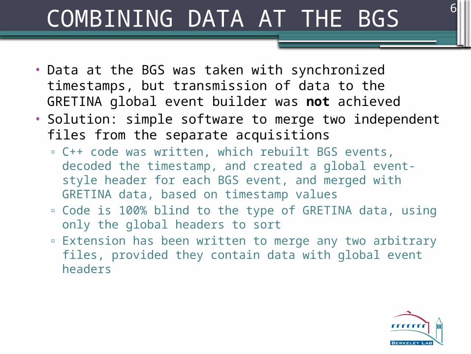
• Data at the BGS was taken with synchronized timestamps, but transmission of data to the GRETINA global event builder was not achieved

• Solution: simple software to merge two independent files from the separate acquisitions▫ C++ code was written, which rebuilt BGS events, decoded the timestamp, and

created a global event-style header for each BGS event, and merged with GRETINA data, based on timestamp values

▫ Code is 100% blind to the type of GRETINA data, using only the global headers to sort

▫ Extension has been written to merge any two arbitrary files, provided they contain data with global event headers

COMBINING DATA AT THE BGS

7

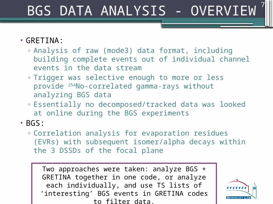
• GRETINA:▫ Analysis of raw (mode3) data format, including building complete

events out of individual channel events in the data stream▫ Trigger was selective enough to more or less provide 254No-

correlated gamma-rays without analyzing BGS data▫ Essentially no decomposed/tracked data was looked at online

during the BGS experiments• BGS:▫ Correlation analysis for evaporation residues (EVRs) with

subsequent isomer/alpha decays within the 3 DSSDs of the focal plane

BGS DATA ANALYSIS - OVERVIEW

Two approaches were taken: analyze BGS + GRETINA together in one code, or analyze each individually, and use TS lists of ‘interesting’ BGS events in GRETINA codes to filter data.

8

• ROOT analysis provides capabilities for full GRETINA analysis, as well as complete BGS (and S800) analysis

• Code is based on global header information –▫ Events are built by grouping global headers within a given time

window (i.e. 10us) – there are no event delineators in the data

▫ Data is handled based on the type given in the global header, making it simple to add auxiliary devices

• ROOT trees allow easy gating on auxiliary detector information to look at GRETINA, etc. – for BGS analysis, multiple trees based on BGS flags sped up spectrum generation, etc.

ROOT CODE ARCHITECTURE

9

• Data analysis at the BGS had a different focus than the analysis here at MSU, or at ANL will have – effort was on optimizing the raw data, identifying and solving problems

• Diagnostic counters were critical:▫40 channels present / crystal (TTCS data taking)▫All channels with a net energy deposition reported it (simple

energy filters checked this for every channel event) – with what frequency was this not true?

▫Does the pile-up flag really tell you about pile-ups on the waveforms? What fraction of events are piled up? CC and segments?

▫ Is the data really time-stamped ordered?• Focus on the use of segment sum energies (as a result of

the high CC rate) led to it’s own set of considerations

BGS DATA ANALYSIS – OPTIMIZING RAW DATA

10

•High CC rates are one instance where using segment sums should provide an advantage in energy resolution (segments won’t be piled-up)

•Not a simple thing to do in practice:▫Segment energy calibrations, especially with non-

linearity of GRETINA ADCs are non-trivial▫Segment integral cross-talk!!!▫Missing segment energies from the FPGA▫Actual detector geometry causing charge loss?

BGS DATA ANALYSIS – SEGMENT SUMS

11 WHY SEGMENT SUMS ARE HARD

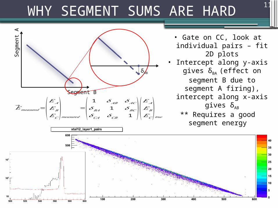
• Gate on CC, look at individual pairs – fit 2D plots

• Intercept along y-axis gives δBA

(effect on segment B due to segment A firing), intercept

along x-axis gives δAB

** Requires a good segment energy calibration

Segm

ent A

Segment B

δAB

�⃗�𝑚𝑒𝑎𝑠𝑢𝑟𝑒𝑑=(𝐸 𝐴

𝐸𝐵

𝐸𝐶)𝑚𝑒𝑎𝑠𝑢𝑟𝑒𝑑

=( 1 𝛿𝐴𝐵 𝛿𝐴𝐶

𝛿𝐵𝐴 1 𝛿𝐵𝐶

𝛿𝐶𝐴 𝛿𝐶𝐵 1 )(𝐸 𝐴

𝐸𝐵

𝐸𝐶)𝑡𝑟𝑢𝑒

12

• While the majority of BGS data analysis effort has not directly translated to the analysis on-going at MSU, it did have a large impact on fixes made to the data acquisition, etc.

• Techniques for calibration and correction important to segment summing will be important in future physics

• campaigns, and • continuing work will • refine the analysis using• segment sums

BGS DATA ANALYSIS – WHERE ARE WE?

13

All told, 7 GRETINA quads provides 1120 electronics channels which need to be calibrated – 112 CC and 1008 segments

Considerations:• Calibration of all channels is required for decomposition, so even if you’re not

going to use segment energies, you need to calibrate the segments

• If you will use segment energies (i.e. at the BGS), you need a good segment calibration – both energy calibrations and cross-talk corrections will be critical for

summing segments with good resolution

GRETINA CALIBRATION

14

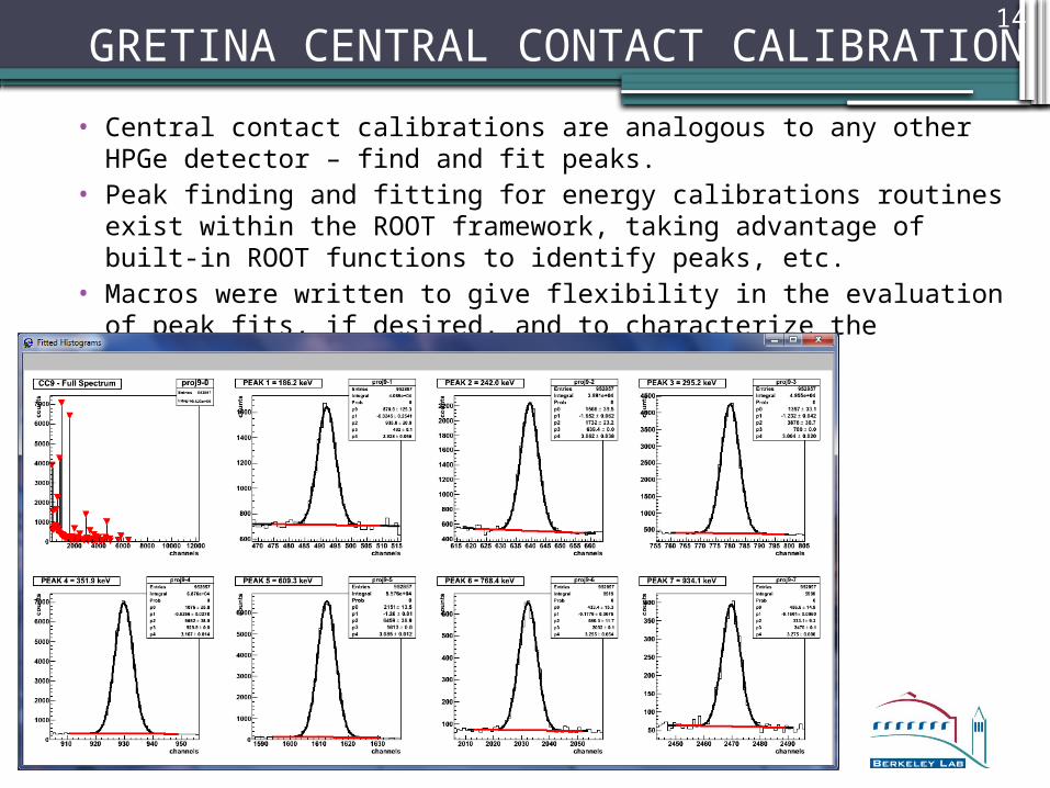
• Central contact calibrations are analogous to any other HPGe detector – find and fit peaks.

• Peak finding and fitting for energy calibrations routines exist within the ROOT framework, taking advantage of built-in ROOT functions to identify peaks, etc.

• Macros were written to give flexibility in the evaluation of peak fits, if desired, and to characterize the detectors in terms of resolution, etc. easily

GRETINA CENTRAL CONTACT CALIBRATION

15

• Segment energy calibrations can be done with an intense 60Co source (or a really long time), but this is a quite limited calibration, at least for rear segments

• As an alternative to a segment calibration based on peak-fitting, segment multiplicity 1 events can provide a method to calibrate

• During the BGS runs, this method provided a superior low-energy calibration, and a first segment non-linearity correction

GRETINA SEGMENT CALIBRATION

16 NON-LINEARITY WOES

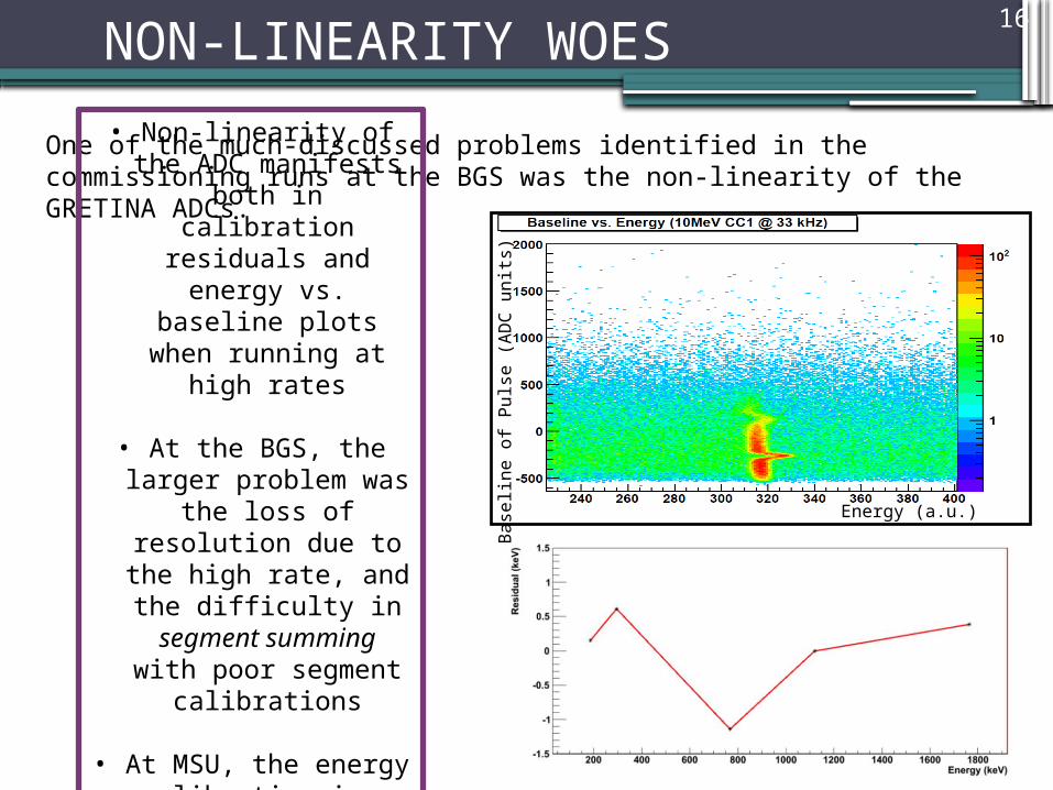
One of the much-discussed problems identified in the commissioning runs at the BGS was the non-linearity of the GRETINA ADCs.

Energy (a.u.)Base

line o

f Puls

e (

AD

C u

nit

s)

• Non-linearity of the ADC manifests both in

calibration residuals and energy vs. baseline plots

when running at high rates

• At the BGS, the larger problem was the loss of

resolution due to the high rate, and the difficulty in segment summing with

poor segment calibrations

• At MSU, the energy calibration is a greater

concern

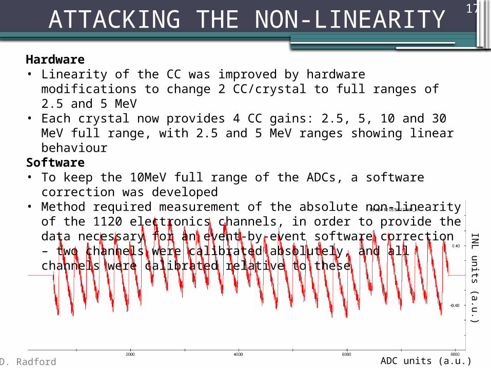
ATTACKING THE NON-LINEARITYHardware• Linearity of the CC was improved by hardware modifications to change 2 CC/crystal

to full ranges of 2.5 and 5 MeV• Each crystal now provides 4 CC gains: 2.5, 5, 10 and 30 MeV full range, with 2.5 and

5 MeV ranges showing linear behaviourSoftware• To keep the 10MeV full range of the ADCs, a software correction was developed• Method required measurement of the absolute non-linearity of the 1120 electronics

channels, in order to provide the data necessary for an event-by-event software correction – two channels were calibrated absolutely, and all channels were calibrated relative to these

D. Radford ADC units (a.u.)

INL units (a.u.)

17

18 ABSOLUTE NON-LINEARITY MEASUREMENT

Delay Amp

ORTEC 427A

Delay Amp

ORTEC 427A

Q1A1 #4Digitizer Module

Triangular wave0.8 V up/down in 0.1 ms1 ms period

Slow ramp-2 -> +2 V, 1.5 s period

ch 0 +

ch 2 +

ch 0 -

ch 2 -

external trigger fromtriangular wave generator

D. Radford

19 ABSOLUTE NON-LINEARITY MEASUREMENT

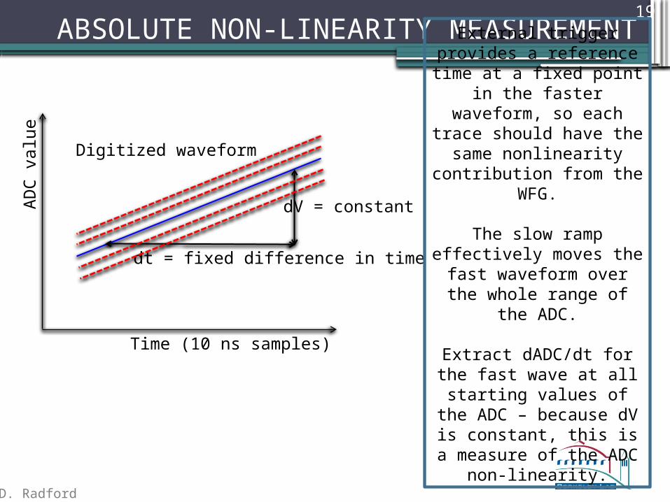
Digitized waveform

ADC

valu

e

Time (10 ns samples)

dV = constant

dt = fixed difference in time

External trigger provides a reference time at a fixed point

in the faster waveform, so each trace should have the

same nonlinearity contribution from the WFG.

The slow ramp effectively moves the fast waveform over the whole range of the ADC.

Extract dADC/dt for the fast wave at all starting values of

the ADC – because dV is constant, this is a measure of

the ADC non-linearity.

D. Radford

20 RELATIVE INTEGRAL NON-LINEARITY MEASUREMENTS

Triangular wave

Refe

renc

e ch

s

Chan

nels

to b

e m

easu

red

Board 1 Board 2

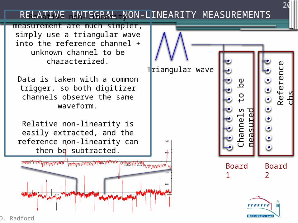
Relative non-linearity measurement are much simpler, simply use a triangular wave into the reference channel + unknown channel to be

characterized.

Data is taken with a common trigger, so both digitizer channels observe the same

waveform.

Relative non-linearity is easily extracted, and the reference non-linearity can then be

subtracted.

D. Radford

21 NON-LINEARITY SOFTWARE CORRECTION

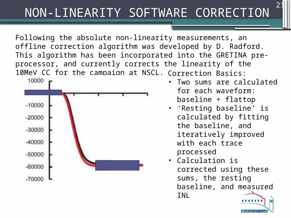
Following the absolute non-linearity measurements, an offline correction algorithm was developed by D. Radford. This algorithm has been incorporated into the GRETINA pre-processor, and currently corrects the linearity of the 10MeV CC for the campaign at NSCL.

Correction Basics:• Two sums are calculated for each

waveform: baseline + flattop • ‘Resting baseline’ is calculated by

fitting the baseline, and iteratively improved with each trace processed

• Calculation is corrected using these sums, the resting baseline, and measured INL

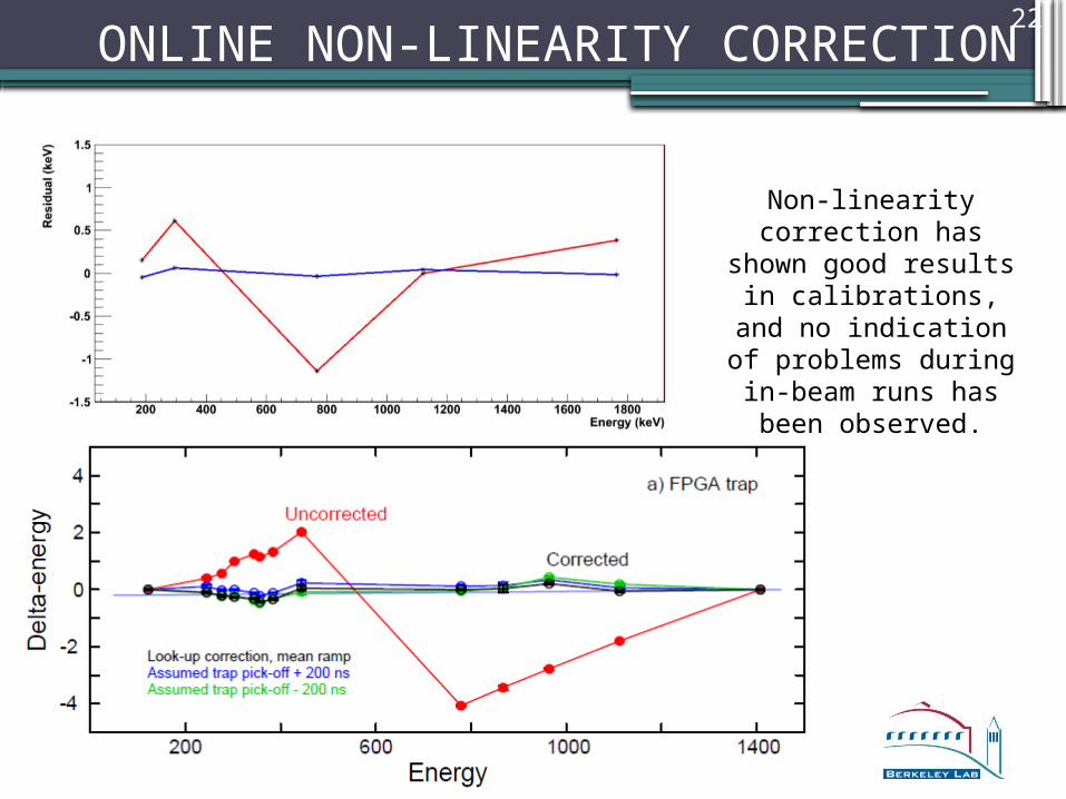
22 ONLINE NON-LINEARITY CORRECTION

Non-linearity correction has shown good results in

calibrations, and no indication of problems

during in-beam runs has been observed.

23

Thank you!

24

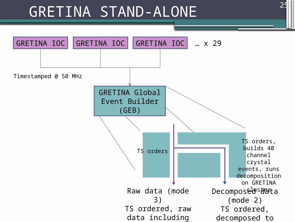
25 GRETINA STAND-ALONE

GRETINA IOCGRETINA IOC … x 29

Timestamped @ 50 MHz

Raw data (mode 3)TS ordered, raw data including waveforms

Decomposed data (mode 2)TS ordered, decomposed to

x,y,z,e

GRETINA IOC

GRETINA Global Event Builder (GEB)

TS orders

TS orders, builds 40 channel crystal

events, runs decomposition on GRETINA cluster

26 GRETINA + S800

Raw data (mode 3)TS ordered, raw data including waveforms

GRETINA ONLY

Decomposed data (mode 2)TS ordered, decomposed to

x,y,z,eGRETINA + S800

TS orders

TS orders, builds 40 channel crystal events, runs decomposition on

GRETINA cluster

The interaction point between the S800 DAQ and GRETINA is at the GEB – S800 events are sent over the network, received and dealt with by the GRETINA GEB. The GEB relies on ‘global headers’ with 3 pieces of information in 16 words:

Type (i.e. 1 = Decomp GRETINA, 2 = Raw GRETINA, etc.)Timestamp (50 MHz)Length of data to follow (in bytes)

S800 CAMAC + VME Readout

GRETINA IOCs

Timestamped @ 12.5 MHz, using GRETINA clock

downscaled by 4

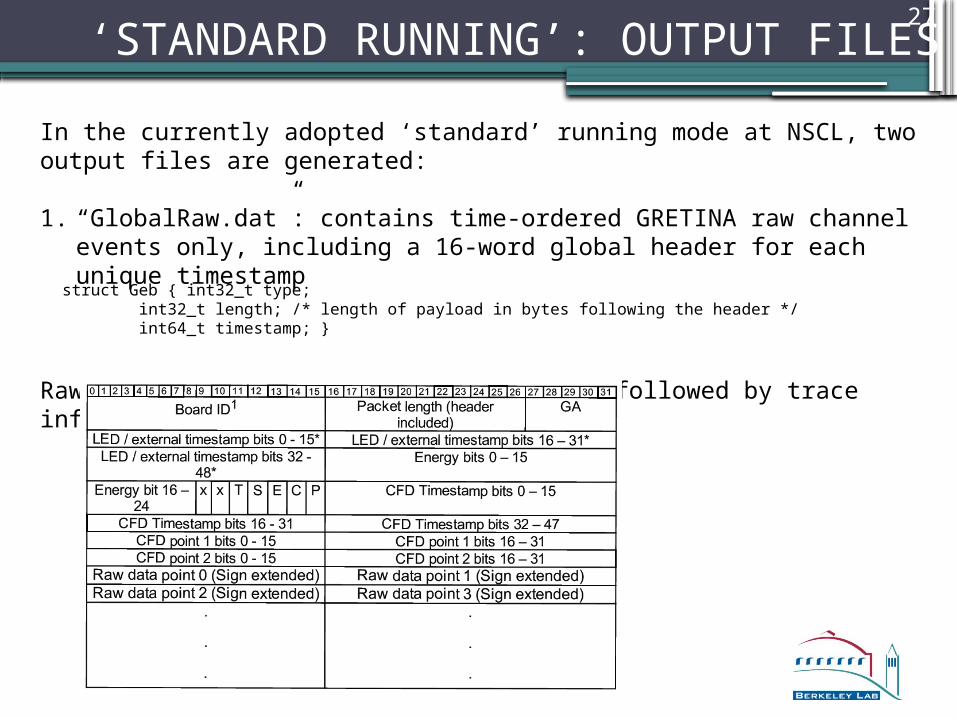
27 ‘STANDARD RUNNING’: OUTPUT FILES

In the currently adopted ‘standard’ running mode at NSCL, two output files are generated:

1. “GlobalRaw.dat”: contains time-ordered GRETINA raw channel events only, including a 16-word global header for each unique timestamp

Raw (Mode 3) data consists of a header, followed by trace information:

struct Geb { int32_t type; int32_t length; /* length of payload in bytes following the header */ int64_t timestamp; }

28 ‘STANDARD RUNNING’: OUTPUT FILES

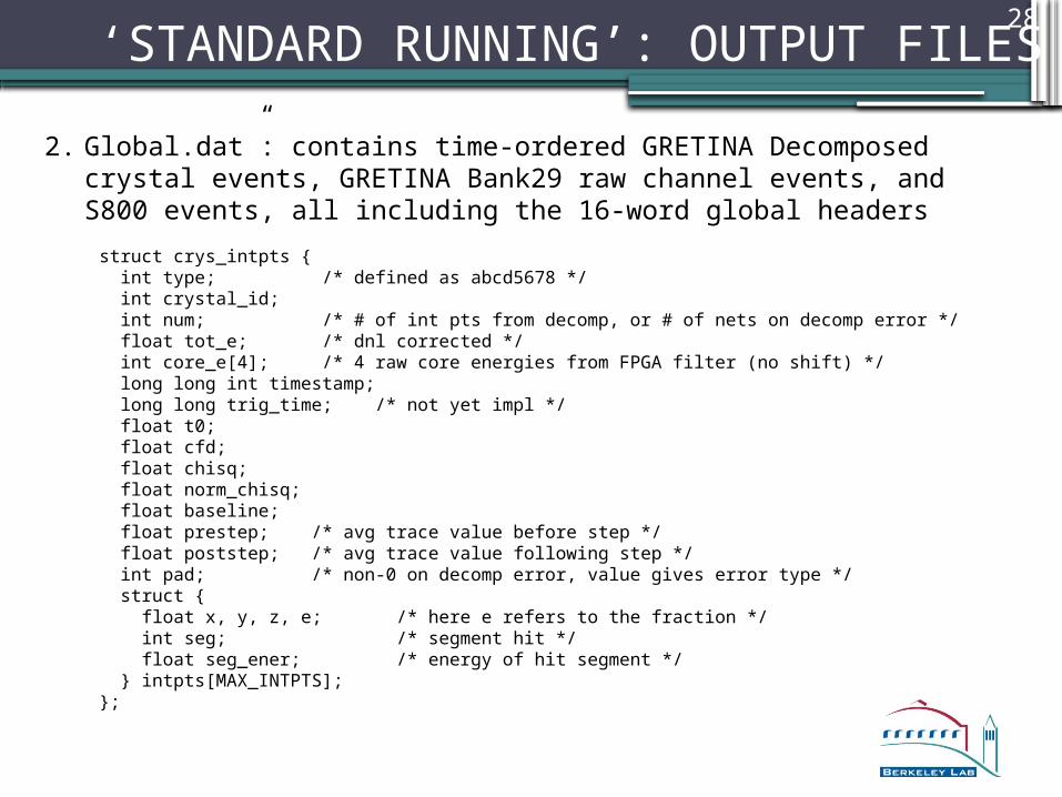
2. Global.dat”: contains time-ordered GRETINA Decomposed crystal events, GRETINA Bank29 raw channel events, and S800 events, all including the 16-word global headers

struct crys_intpts { int type; /* defined as abcd5678 */ int crystal_id; int num; /* # of int pts from decomp, or # of nets on decomp error */ float tot_e; /* dnl corrected */ int core_e[4]; /* 4 raw core energies from FPGA filter (no shift) */ long long int timestamp; long long trig_time; /* not yet impl */ float t0; float cfd; float chisq; float norm_chisq; float baseline; float prestep; /* avg trace value before step */ float poststep; /* avg trace value following step */ int pad; /* non-0 on decomp error, value gives error type */ struct { float x, y, z, e; /* here e refers to the fraction */ int seg; /* segment hit */ float seg_ener; /* energy of hit segment */ } intpts[MAX_INTPTS];};

29 ONLINE DAQ MONITORING - GRETINA

Effort has been put in to distill the large amount of DAQ information available in EPICS to the key information, and consolidate this onto one meaningful alarm page.

30 ONLINE DATA INTEGRITY MONITORING

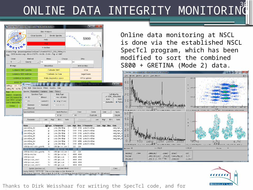
Online data monitoring at NSCL is done via the established NSCL SpecTcl program, which has been modified to sort the combined S800 + GRETINA (Mode 2) data.

Thanks to Dirk Weisshaar for writing the SpecTcl code, and for the screenshots.

31 DATA ANALYSISOnline:Online data analysis at NSCL is essentially restricted to SpecTcl. All other software analyzes files written to disk.

Offline: At present, there is no officially supported offline analysis package for GRETINA data, however there are several options to start users off.

1. SpecTcl – the same code used for online analysis can be used offline. There are possibilities using SpecTcl to create intermediate output files, with S800 physics data processed into a simplified format, and GRETINA left intact. NSCL / Dirk Weisshaar

2. C unpackers – for GRETINA only, there exist straightforward C codes which typically fill RadWare spectra. These are an excellent starting point for a user who prefers to stay away from SpecTcl/ROOT. Paul Fallon / David Radford

3. ROOT – at present, two independent ROOT analysis codes exist, which analyze both S800 + GRETINA (Mode2/Mode3). One code has the possibility of tracking included. Heather Crawford / Kathrin Wimmer (code available at http://www.nscl.msu.edu/~wimmer/software.php -- password by emailing Kathrin at wimme1k@cmich.edu)

32 DATA ANALYSIS – OFFLINE WITH ROOT

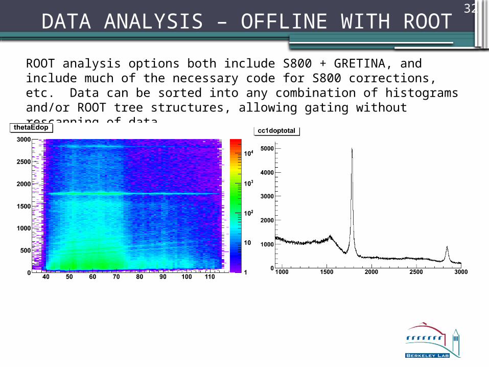
ROOT analysis options both include S800 + GRETINA, and include much of the necessary code for S800 corrections, etc. Data can be sorted into any combination of histograms and/or ROOT tree structures, allowing gating without rescanning of data.

33 DATA ANALYSIS – TRACKING

Tracking is currently not being done online, but rather as a part of the offline data analysis. The supported tracking code comes from Torben Lauritsen, and uses ROOT to generate histograms, and write a tracked output file, which builds events and returns GRETINA in Mode1, or tracked format.

Eg

At present, Torben’s code can handle BGS data, and enhancements for S800 analysis (with S800physics) are underway.

http://www.phy.anl.gov/gretina