Bidirectional Conditional Insertion Sort algorithm; An efficient progress on the classicalinsertion sort

Adnan Saher Mohammeda,∗, Sahin Emrah Amrahovb, Fatih V. Celebic

aYıldırım Beyazıt University, Graduate School of Natural Sciences, Computer Engineering Dept., Ankara, Turkeyb Ankara University, Faculty of Engineering, Computer Engineering Dept., Ankara, Turkey

cYıldırım Beyazıt University, Faculty of Engineering and Natural Sciences, Computer Engineering Dept., Ankara, Turkey

Abstract

In this paper, we proposed a new efficient sorting algorithm based on insertion sort concept. The proposed algorithm called Bidirec-tional Conditional Insertion Sort (BCIS). It is in-place sorting algorithm and it has remarkably efficient average case time complexitywhen compared with classical insertion sort (IS). By comparing our new proposed algorithm with the Quicksort algorithm, BCISindicated faster average case time for relatively small size arrays up to 1500 elements. Furthermore, BCIS was observed to be fasterthan Quicksort within high rate of duplicated elements even for large size array.

Keywords: insertion sort, sorting, Quicksort, bidirectional insertion sort

1. Introduction

Algorithms have an important role in developing process ofcomputer science and mathematics. Sorting is a fundamen-tal process in computer science which is commonly used forcanonicalizing data. In addition to the main job of sorting al-gorithms, many algorithms use different techniques to sort listsas a prerequisite step to reduce their execution time [20]. Theidea behind using sorting algorithms by other algorithm is com-monly known as reduction process. A reduction is a methodfor transforming one problem to another easier than the firstproblem [32]. Consequently, the need for developing efficientsorting algorithms that invest the remarkable development incomputer architecture has increased.

Sorting is generally considered to be the procedure of reposi-tioning a known set of objects in ascending or descending orderaccording to specified key values belong to these objects. Sort-ing is guaranteed to finish in finite sequence of steps[8].

Among a large number of sorting algorithms, the choice ofwhich is the best for an application depends on several factorslike size, data type and the distribution of the elements in a dataset. Additionally, there are several dynamic influences on theperformance of the sorting algorithm which it can be briefed asthe number of comparisons (for comparison sorting), number ofswaps (for in-place sorting),memory usage and recursion [1].

Generally, the performance of algorithms measured by thestandard Big O(n) notation which is used to describe the com-plexity of an algorithm. Commonly, sorting algorithms hasbeen classified into two groups according to their time complex-ity. The first group is O(n2) which contains the insertion sort,

∗Corresponding authorEmail addresses: adnshr@gmail.com (Adnan Saher Mohammed),

emrah@eng.ankara.edu.tr (Sahin Emrah Amrahov),fvcelebi@ybu.edu.tr (Fatih V. Celebi)

selection sort, bubble sort etc. The second group is O(n log n),which is faster than the first group, includes Quicksort ,mergesort and heap sort [12]. The insertion sort algorithm can beconsidered as one of the best algorithms in its family (O(n2)group ) due to its performance, stable algorithm ,in-place, andsimplicity [34]. Moreover, it is the fastest algorithm for smallsize array up to 28-30 elements compared to the Quicksort algo-rithm. That is why it has been used in conjugate with Quicksort[30, 31, 36, 4] .

Several improvements on major sorting algorithms have beenpresented in the literature [22, 9, 29]. Chern and Hwang [7]give an analysis of the transitional behaviors of the average costfrom insertion sort to quicksort with median-of-three. Fouz etal [13] provide a smoothed analysis of Hoare’s algorithm whohas found the quicksort. Recently, we meet some investiga-tions of the dual-pivot quicksort which is the modification ofthe classical quicksort algorithm. In the partitioning step of thedual-pivot quicksort two pivots are used to split the sequenceinto three segments recursively. This can be done in differentways. Most efficient algorithm for the selection of the dual-pivot is developed due to Yaroslavskiy question [37]. Nebel,Wild and Martinez [24] explain the success of Yaroslavskiy’snew dual-pivot Quicksort algorithm in practice. Wild and Nebel[35] analyze this algorithm and show that on average it uses1.9n ln n + O(n) comparisons to sort an input of size n, beat-ing standard quicksort, which uses 2n ln n + O(n) comparisons.Aumuller and Dietzfelbinger [2] propose a model that includesall dual-pivot algorithms, provide a unified analysis, and iden-tify new dual-pivot algorithms for the minimization of the aver-age number of key comparisons among all possible algorithms.This minimum is 1.8n ln n + O(n). Fredman [14] presents anew and very simple argument for bounding the expected run-ning time of Quicksort algorithm. Hadjicostas and Lakshmanan[17] analyze the recursive merge sort algorithm and quantify

Preprint submitted to Future Generation Computer Systems August 16, 2016

arX

iv:1

608.

0261

5v2

[cs

.DS]

12

Aug

201

6

the deviation of the output from the correct sorted order if theoutcomes of one or more comparisons are in error. Bindjemeand Fill [6] obtain an exact formula for the L2-distance of the(normalized) number of comparisons of Quicksort under theuniform model to its limit. Neininger [25] proves a centrallimit theorem for the error and obtain the asymptotics of theL3−distance. Fuchs [15] uses the moment transfer approach tore-prove Neininger’s result and obtains the asymptotics of theLp − distance for all 1 ≤ p < ∞.

Grabowski and Strzalka [16] investigate the dynamic behav-ior of simple insertion sort algorithm and the impact of long-term dependencies in data structure on sort efficiency. Bier-nacki and Jacques [5] propose a generative model for rank databased on insertion sort algorithm. The work that presentedin [3] is called library sort or gapped insertion sort which istrading-off between the extra space used and the insertion time,so it is not in-place sorting algorithm. The enhanced insertionsort algorithm that presented in [33] is use approach similar tobinary insertion sort in [27], whereas both algorithms reducedthe number of comparisons and kept the number of assign-ments (shifting operations) equal to that in standard insertionsort O(n2). Bidirectional insertion sort approaches presented in[8, 11]. They try to make the list semi sorted in Pre-processingstep by swapping the elements at analogous positions (position1 with n, position 2 with (n-1) and so on). Then they apply thestandard insertion sort on the whole list. The main goal of thiswork is only to improve worst case performance of IS [11] . Onother hand, authors in[34] presented a bidirectional insertionsort, firstly exchange elements using the same way in [8, 11], then starts from the middle of the array and inserts elementsfrom the left and the right side to the sorted portion of the mainarray. This method improves the performance of the algorithmto be efficient for small arrays typically of size lying from 10-50elements [34] . Finally, the main idea of the work that presentedin [23], is based on inserting the first two elements of the un-ordered part into the ordered part during each iteration. Thisidea earned slightly time efficient but the complexity of the al-gorithm still O(n2) [23] . However, all the cited previous workshave shown a good enhancement in insertion sort algorithm ei-ther in worst case, in large array size or in very small array size.In spite of this enhancement, a Quicksort algorithm indicatesfaster results even for relatively small size array.

In this paper, a developed in-place unstable algorithm is pre-sented that shows fast performance in both relatively small sizearray and for high rate duplicated elements array. The proposedalgorithm Bidirectional Conditional Insertion Sort (BCIS) iswell analyzed for best, worst and average cases. Then it is com-pared with well-known algorithms which are classical InsertionSort (IS) and Quicksort. Generally, BCIS has average timecomplexity very close to O(n1.5) for normally or uniformly dis-tributed data. In other word, BCIS has faster average case thanIS for both relatively small and large size array. Additionally,when it compared with Quicksort, the experimental results forBCIS indicates less time complexity up to 70% -10% withinthe data size range of 32-1500. Besides, our BCIS illustratesfaster performance in high rate duplicated elements array com-pared to the Quicksort even for large size arrays. Up to 10%-

50% is achieved within the range of elements of 28-more than3000000. The other pros of BCIS that it can sort equal elementsarray or remain equal part of an array in O(n) .

This paper is organized as follows: section-2 presents theproposed algorithm and pseudo code, section-3 executes theproposed algorithm on a simple example array, section-4 illus-trates the detailed complexity analysis of the algorithm, section-5 discusses the obtained empirical results and compares themwith other well-known algorithms, section-6 provides conclu-sions. Finally, you will find the important references.

2. The proposed algorithm BCIS

The classical insertion sort explained in [23, 19, 26] has onesorted part in the array located either on left or right side. Foreach iteration, IS inserts only one item from unsorted part intoproper place among elements in the sorted part. This processrepeated until all the elements sorted.

Our proposed algorithm minimizes the shifting operationscaused by insertion processes using new technique. This newtechnique supposes that there are two sorted parts located at theleft and the right side of the array whereas the unsorted partlocated between these two sorted parts. If the algorithm sortsascendingly, the small elements should be inserted into the leftpart and the large elements should be inserted into the rightpart. Logically, when the algorithm sorts in descending order,insertion operations will be in reverse direction. This is the ideabehind the word bidirectional in the name of the algorithm.

Unlike classical insertion sort, insertion items into two sortedparts helped BCIS to be cost effective in terms of memoryread/write operations. That benefit happened because the lengthof the sorted part in IS is distributed to the two sorted parts inBCIS. The other advantage of BCIS algorithm over classicalinsertion sort is the ability to insert more than one item in theirfinal correct positions in one sort trip (internal loop iteration).

Additionally, the inserted items will not suffer from shift-ing operations in later sort trips. Alongside, insertion into bothsorted sides can be run in parallel in order to increase the algo-rithm performance (parallel work is out of scope of this paper).

In case of ascending sort, BCIS initially assumes that themost left item at array[1] is the left comparator (LC) whereis the left sorted part begin. Then inserts each element intothe left sorted part if that element less than or equal to the LC.Correspondingly, the algorithm assumes the right most item atarray[n] is the right comparator (RC) which must be greaterthan LC. Then BCIS inserts each element greater than or equalto the RC into the right sorted part. However, the elements thathave values between LC and RC are left in their positions dur-ing the whole sort trip. This conditional insertion operation isrepeated until all elements inserted in their correct positions.

If the LC and RC already in their correct position, there areno insertion operations occur during the whole sort trip. Hence,the algorithm at least places two items in their final correct po-sition for each iteration.

In the pseudo code (part 1& 2), the BCIS algorithm is pre-sented in a format uses functions to increase the clarity and

2

traceability of the algorithm. However, in statements (1 & 2)the algorithm initially sets two indexes, SL for the sorted leftpart and SR for the sorted right part to indicate on the most leftitem and the most right item respectively.

Algorithm BCIS Part 1 (Main Body)1: S L← le f t2: S R← right3: while S L < S R do4: SWAP(array, S R, S L +

(S R−S L)2 )

5: if array[S L] = array[S R] then6: if ISEQUAL(array, S L, S R)=-1 then7: return8: end if9: end if

10: if array[SL] > array[SR] then11: SWAP (array, SL , SR)12: end if13: if (S R − S L) ≥ 100 then14: for i← S L + 1 to (S R − S L)0.5 do15: if array[SR] < array[i] then16: SWAP (array, SR, i)17: else if array[SL] > array[i] then18: SWAP (array, SL, i)19: end if20: end for21: else22: i← S L + 123: end if24: LC ← array[S L]25: RC ← array[S R]26: while i < S R do27: CurrItem← array[i]28: if CurrItem ≥ RC then29: array[i]← array[S R − 1]30: INS RIGHT (array,CurrItem, S R, right)31: S R← S R − 132: else if CurrItem ≤ LC then33: array[i]← array[S L + 1]34: INS LEFT (array,CurrItem, S L, le f t)35: S L← S L + 136: i← i + 137: else38: i← i + 139: end if40: end while41: S L← S L + 142: S R← S R − 143: end while

The main loop starts at statements(3) and stops when the leftsorted part index (SL) reaches the right sorted part index (SR).

The selection of LC and RC is processed by the statements(4-25). In order to ensure the correctness of the insertion op-erations LC must be less than RC, this condition processed instatement (5). In case of LC equal to RC, the statement (6), us-ing ISEQUAL function, tries to find an item not equal to LC and

Algorithm BCIS Part 2 (Functions)44: function ISEQUAL(array, S L, S R)45: for k ← S L + 1 to S R − 1 do46: if array[k]! = array[S L] then47: S WAP(array, k, S L)48: return k49: end if50: end for51: return − 152: . End the algorithm because all scanned items are equal53: end function54: function InsRight(array,CurrItem, S R, right)55: j← S R56: while j ≤ right and CurrItem > array[ j] do57: array[ j − 1]← array[ j]58: j← j + 159: end while60: Array[ j − 1]← CurrItem61: end function62: function InsLeft(array,CurrItem, S L, le f t)63: j← S L64: while j ≥ le f t and CurrItem < array[ j] do65: array[ j + 1]← array[ j]66: j← j − 167: end while68: Array[ j + 1]← CurrItem69: end function70: function SWAP(array,i,j)71: Temp← array[i]72: array[i]← array[ j]73: array[ j]← Temp74: end function

replace it with LC. Otherwise, (if not found) all remaining ele-ments in the unsorted part are equal. Thus, the algorithm shouldterminate at the statement (7). Furthermore, this technique al-lows equal elements array to sort in only O(n) time complexity.Statements (4 & 13 – 20) do not have an effect on the correct-ness of the algorithm, these statements are added to enhancethe performance of the algorithm. The advantage of these tech-niques will be discussed in the analysis section (section-4).

The while statement in (26) is the beginning of the sort trip,as mentioned previously, conditional insertions occur insidethis loop depending on the value of current item (CurrItem)in comparison with the values of LC and RC. Insertion opera-tions are implemented by calling the functions INSRIGHT andINSLEFT.

3. Example

The behavior of the proposed algorithm on an array of 15elements generated randomly by computer is explained in Fig-ure(1). In order to increase the simplicity of this example, weassumed the statements (4 & 13-20) do not exist in the algo-rithm. For all examples in this paper we assumed as follows:Items in red color mean these items are currently in process.

3

Bolded items represent LC and RC for current sort trip. Graybackground means the position of these items may change dur-ing the current sort trip. Finally, items with green backgroundmean these items are in their final correct positions.

First sort trip starts here

Insert into the left

No insertion

No insertion

No insertion

No insertion

Insert into the right

Insert into the right

No insertion

Insert into the right

No insertion

Insert into the right

No insertion

Insert into the left

End of first sort trip.

Check LC and RC, swap

Second sort trip starts here

Insert into the left

Insert into the right

Insert into the left

Insert into the right

Insert into the left

End of second sort trip, all items has been sorted

17 19 22 28 52 53 56 57 59 65 67 72 73 78 80

22 17 56 57 52 59 80 78 73 19 53 28 65 72 67

17 22 56 57 52 59 80 78 73 19 53 28 65 72 67

17 22 56 57 52 59 80 78 73 19 53 28 65 72 67

17 22 56 57 52 59 80 78 73 19 53 28 65 72 67

17 22 56 57 52 59 80 78 73 19 53 28 65 72 67

17 22 56 57 52 59 80 78 73 19 53 28 65 72 67

17 22 56 57 52 59 72 78 73 19 53 28 65 67 80

17 22 56 57 52 59 65 78 73 19 53 28 67 72 80

17 22 56 57 52 59 65 78 73 19 53 28 67 72 80

17 22 56 57 52 59 65 28 73 19 53 67 72 78 80

17 22 56 57 52 59 65 28 73 19 53 67 72 78 80

17 22 56 57 52 59 65 28 53 19 67 72 73 78 80

17 22 56 57 52 59 65 28 53 19 67 72 73 78 80

17 19 22 57 52 59 65 28 53 56 67 72 73 78 80

17 19 22 56 52 59 65 28 53 57 67 72 73 78 80

17 19 22 52 56 59 65 28 53 57 67 72 73 78 80

17 19 22 52 56 53 65 28 57 59 67 72 73 78 80

17 19 22 52 53 56 65 28 57 59 67 72 73 78 80

17 19 22 52 53 56 28 57 59 65 67 72 73 78 80

Figure 1: BCIS Example

4. Analysis of The Proposed Algorithm

The complexity of the proposed algorithm mainly dependson the complexity of insertion functions which is in turn de-pends on the number of inserted elements in each function dur-ing each sorting trip. To explain how the performance of BCISdepends on the number of inserted element per each sort trip,several assumptions are presented which revealed theoreticalanalysis very close to experiential results that we obtained.

In order to simplify the analysis, we will concentrate on themain parts of the algorithm. Assume that during each sort trip(k) elements are inserted into both sides, each side get k/2.Whereas insertion functions work exactly like standard inser-tion sort. Consequently, time complexity of each sort trip equalto the sum of the left and right insertion function cost whichis equal to Tis(k/2) for each function, in addition to the cost ofscanning of the remaining elements (not inserted elements). Wecan express this idea as follows :-

T (n) = Tis(k2

) + Tis(k2

) + 2(n − k)

+ Tis(k2

) + Tis(k2

) + 2(n − 2k)

+ Tis(k2

) + Tis(k2

) + 2(n − 3k)

+ · · · + Tis(k2

) + Tis(k2

) + 2(n − ik)

BCIS stops when n − ik = 0 =⇒ i = nk

T (n) =nk

[Tis(

k2

) + Tis(k2

)]

+

nk∑

i=1

(n − ik) (1)

=nk

[Tis(

k2

) + Tis(k2

)]

+n2

k− n

=nk

[Tis(

k2

) + Tis(k2

) + n]− n (2)

Equation (2) represents a general form of growth function,it shows that the complexity of the proposed algorithm mainlydepends on the value of k and the complexity of insertion func-tions.

4.1. Average Case Analysis

The average case of classical insertion sort Tis(n) that ap-peared in equation (2) has been well analyzed in terms of com-parisons in [28, 21] and in [21] for assignments. However,authors of the cited works presented the following equationswhich represent the average case analysis for classical insertionsort for comparisons and assignments respectively.

Tisc(n) =n2

4+

3n4− 1 (3)

Tisa(n) =n2

4+

7n4

+ 3 (4)

The equations (3 & 4) show that the insertion sort has ap-proximately equal number of comparisons (Tisc(n)) and assign-ments (Tisa(n)). However, for BCIS, it is assumed that in eachsort trip k elements are inserted into both side. Therefore, themain while loop executes n/k times that represent the numberof sort trips. Suppose each insertion function get k/2 elementswhere 2 ≤ k ≤ n. Since both insertion functions (INSLEFT,INSRIGHT) exactly work as a standard insertion sort, so theaverage case for each function during each sort trip is .

Comp.#/S ortTrip/Function = Tisc(k2

)

=k2

16+

3k8− 1 (5)

BCIS performs one extra assignment operation to move theelement that neighbored to the sorted section before callingeach insertion function. Considering this cost we obtained asfollows: -

Assig.#/S ortTrip/Function = Tisa(k2

) + 1

=k2

16+

7k8

+ 4 (6)

4

In order to compute BCIS comparisons complexity, wesubstituted equation (5) in equation (2) and we obtained asfollows:-

Tc(n) =nk

[k2

8+

3k4− 2 + n

]− n (7)

Equation (7) shows that when k gets small value the algo-rithm performance goes close to O(n2). For k = 2 the growthfunction is shown below.

Tc(n) =n2

[48

+32− 2 + n

]− n

=n2

2− n (8)

When k gets large value also the complexity of BCIS goesclose to O(n2). For k=n the complexity is:-

Tc(n) =nn

[n2

8+

3n4− 2 + n

]− n

=n2

8+

3n4− 2 (9)

Hence, the approximate best performance of the average casefor BCIS that could be obtained when k = n0.5 as follows:-

Tc(n) =n

n0.5

[n8

+3n0.5

4− 2 + n

]− n

=9n1.5

8−

n4− 2n0.5 (10)

Equation(10) computes the number of comparisons of BCISwhen runs in the best performance of the average case. On otherhand, to compute the the number of assignments for BCIS incase of best performance of average case. Since assignmentsoperations occur only in insertions functions, equation (6) ismultiplied by two because there are two insertion functions,then the result is multiplied by the number of sort trip n

k . Whenk = n0.5 we got as follows:

Ta(n) =n

n0.5

[n8

+7n0.5

4+ 8

]=

n1.5

8+

7n4

+ 8n0.5 (11)

The comparison of equation (10) with equation (11) provesthat the number of assignments less than the number of compar-isons in BCIS. As we mentioned previously in equations(3 &4), IS has approximately equal number of comparisons and as-signments. This property makes BCIS runs faster than IS evenwhen they have close number of comparisons.

Hence, we wrote the code section in statements (13-20) tooptimize the performance of BCIS by keeping k close to n0.5

as possible. This code segment is based on the idea that en-sures at least a set of length (S R − S L)0.5 not to be insertedduring the current sort trip (where sort trip size = SR-SL). Thisidea realized by scanning this set looking for the minimum and

maximum element and replace them with LC and RC respec-tively. However, this code does not add extra cost for the per-formance of the algorithm because the current sort trip will startwhere the loop in statement (14 ) has finished (sort trip will startat (S R − S L)0.5 + 1). Theoretical results have been comparedwith experimental results in section-5 and BCIS showed per-formance close to the best performance of average case thatexplained above.

In the rest part of this section, instruction level analysis ofBCIS is presented. We re-analyze the algorithm for averagecase by applying above assumption to get more detailed anal-ysis. However, the cost of each instruction is demonstrated ascomment in the pseudo code of the algorithm, we do not ex-plicitly calculate the cost of the loop in statement (14), becauseit is implicitly calculated with the cost of not inserted elementsinside the loop started in statement (25). Code segment withinstatements (13-20) activates for sort trip size greater than 100elements only. Otherwise, sort trip index i starts from the ele-ment next to SL (statement 22).

The total number of comparisons for each insertion functionis calculated by equation(5) multiplied by the number of sorttrip (n/k) as following:-

nk

(k2

16+

3k8− 1

)=

nk16

+3n8−

nk

(12)

The Complexity of the check equality function ISEQUAL isneglected because if statement at (5) rarely gets true. The totalcomplexity of BCIS is calculated as following:-

Algorithm BCIS Average case analysis Part 11: S L← le f t . C12: S R← right . C23: while S L < S R do . C3( n

k + 1)4: SWAP(array, S R, S L +

(S R−S L)2 ) . C4( n

k )5: if array[S L]= array[S R] then . C5( n

k )6: if ISDUP(array, S L, S R)=-1 then7: return8: end if9: end if

10: if array[SL] > array[SR] then . C6( nk )

11: SWAP (array, SL , SR)12: end if13: if (S R − S L) ≥ 100 then . C7( n

k )14: for i← S L + 1 to (S R − S L)0.5 do15: if array[SR] < array[i] then16: SWAP (array, SR, i)17: else if array[SL] > array[i] then18: SWAP (array, SL, i)19: end if20: end for21: else22: i← S L + 123: end if24: LC ← array[S L] . C8( n

k )25: RC ← array[S R] . C9( n

k )

5

Algorithm BCIS Average case analysis Part 2

26: while i < S R do . C10∑ n

ki=1(n − ik)

27: CurrItem← array[i] . C11∑ n

ki=1(n − ik)

28: if CurrItem ≥ RC then . C12∑ n

ki=1(n − ik)

29: array[i]← array[S R − 1] . C13( n2 )

30: INS RIGHT (array,CurrItem, S R, right) . C14( nk

16 + 3n8 −

nk )

31: S R← S R − 1 . C15( n2 )

32: else if CurrItem ≤ LC then . C16(∑ n

ki=1(n − ik) − n

2 )33: array[i]← array[S L + 1] . C17( n

2 )34: INS LEFT (array,CurrItem, S L, le f t) . C14

( nk16 + 3n

8 −nk )

35: S L← S L + 1 . C18( n2 )

36: i← i + 1 . C19( n2 )

37: else38: i← i + 1 . C20(

∑ nki=1(n − ik) − n)

39: end if40: end while41: S L← S L + 1 . C19( n

k )42: S R← S R − 1 . C19( n

k )43: end while

T (n) = C1 + C2 + C3

+ (C3 + C4 + C5 + C6 + C7 + C8 + C21 + C22)nk

+ (C10 + C11 + C12 + C16 + C20)

nk∑

i=1

(n − ik)

+ (C13 + C15 −C16 + C17 + C18 + C19)nk

+ C14 ∗ 2(

nk16

+3n8−

nk

)−C20n

a = (C3 + C4 + C5 + C6 + C7 + C8 + C21 + C22)b = C14c = (C10 + C11 + C12 + C16 + C20)d = (C13 + C15 −C16 + C17 + C18 + C19)e = C20f = (C1 + C2 + C3)

T (n) = ank

+ b(

nk8

+3n4−

nk

)+ c

nk∑

i=1

(n − ik)

+ dn2− en + f

= ank

+ b(

nk8

+3n4−

nk

)+ c

(n2

2k−

n2

)+ d

n2− en + f

=nk

[a + b

(k8

+3k4− 2

)+ c

n2

]− c

n2

+ dn2− en + f (13)

We notice that equation (13) is similar to equation (7) whenconstants represent instructions cost.

4.2. Best Case Analysis

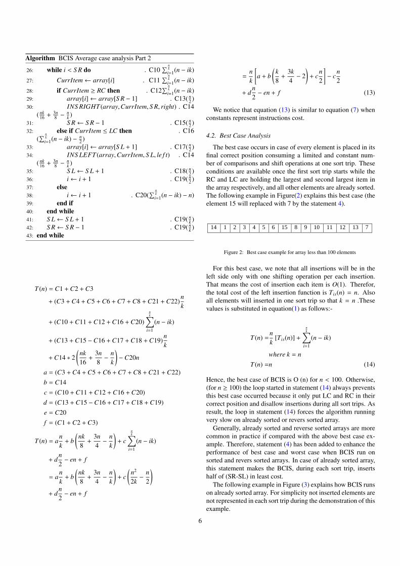
The best case occurs in case of every element is placed in itsfinal correct position consuming a limited and constant num-ber of comparisons and shift operations at one sort trip. Theseconditions are available once the first sort trip starts while theRC and LC are holding the largest and second largest item inthe array respectively, and all other elements are already sorted.The following example in Figure(2) explains this best case (theelement 15 will replaced with 7 by the statement 4).

14 1 2 3 4 5 6 15 8 9 10 11 12 13 7

Figure 2: Best case example for array less than 100 elements

For this best case, we note that all insertions will be in theleft side only with one shifting operation per each insertion.That means the cost of insertion each item is O(1). Therefor,the total cost of the left insertion function is Tis(n) = n. Alsoall elements will inserted in one sort trip so that k = n .Thesevalues is substituted in equation(1) as follows:-

T (n) =nk

[Tis(n)] +

nk∑

i=1

(n − ik)

where k = n

T (n) =n (14)

Hence, the best case of BCIS is O (n) for n < 100. Otherwise,(for n ≥ 100) the loop started in statement (14) always preventsthis best case occurred because it only put LC and RC in theircorrect position and disallow insertions during all sort trips. Asresult, the loop in statement (14) forces the algorithm runningvery slow on already sorted or revers sorted array.

Generally, already sorted and reverse sorted arrays are morecommon in practice if compared with the above best case ex-ample. Therefore, statement (4) has been added to enhance theperformance of best case and worst case when BCIS run onsorted and revers sorted arrays. In case of already sorted array,this statement makes the BCIS, during each sort trip, insertshalf of (SR-SL) in least cost.

The following example in Figure (3) explains how BCIS runson already sorted array. For simplicity not inserted elements arenot represented in each sort trip during the demonstration of thisexample.

6

Original array.

Statement 4.

1st sort trip.

Insertions started.

Statement 4.

2nd sort trip.

Insertions started.

Statement 10, no swap.

1 2 3 4 5 6 7 8 9 10 11 12 13 14 15 16

1 2 3 4 5 6 7 8 16 10 11 12 13 14 15 9

1 2 3 4 5 6 7 8 16 10 11 12 13 14 15 9

1 2 3 4 5 6 7 8 15 10 11 12 13 14 9 16

1 2 3 4 5 6 7 8 14 10 11 12 13 9 15 16

1 2 3 4 5 6 7 8 13 10 11 12 9 14 15 16

1 2 3 4 5 6 7 8 12 10 11 9 13 14 15 16

1 2 3 4 5 6 7 8 11 10 9 12 13 14 15 16

1 2 3 4 5 6 7 8 10 9 11 12 13 14 15 16

1 2 3 4 5 6 7 8 9 10 11 12 13 14 15 16

1 2 3 4 5 6 7 8 9 10 11 12 13 14 15 16

1 2 3 4 8 6 7 5 9 10 11 12 13 14 15 16

1 2 3 4 7 6 5 8 9 10 11 12 13 14 15 16

1 2 3 4 6 5 7 8 9 10 11 12 13 14 15 16

1 2 3 4 5 6 7 8 9 10 11 12 13 14 15 16

1 2 3 4 5 6 7 8 9 10 11 12 13 14 15 16

1 2 3 4 5 6 7 8 9 10 11 12 13 14 15 16

Figure 3: Example of running BCIS on already sorted array

For already sorted array, BCIS scans the first half consumingtwo comparisons per item (no insertions), then inserts the sec-ond half of each sort trip consuming two comparisons per itemtoo. Because the sort trip size is repeatedly halved. Hence, itcan represent as following.

T (n) =

(2

n2

+ 2n2

)+

(2

n4

+ 2n4

)+

(2

n8

+ 2n8

)+ ..... +

(2

n2i + 2

n2i

)stop when 2i = n =⇒ i = log n

T (n) =

log n∑i=1

(2n2i + 2

n2i ) = 4n (15)

Equations (14 & 15) represent the best case growth functionsof BCIS when run on array size less than 100 and greater thanand equal to 100 respectively.

4.3. Worst Case Analysis

The worst case happens only if all elements are inserted inone side in reverse manner during the first sort trip. This con-dition provided when the RC and LC are the largest and secondlargest numbers in the array respectively, and all other itemsare sorted in reverse order. The insertion will be in the left sideonly. The following example in Figure(4) explains this worstcase when n < 100.

14 13 12 11 10 9 8 15 6 5 4 3 2 1 7

Figure 4: Worst case example for array less than 100 elements

Since each element in the this example inserted reversely, thecomplexity of left insertion function for each sort trip equal toTis(n) =

n(n−1)2 . Also there is one sort trip so k = n, by substitute

these values in equation(1) as follows :-

T (n) =nk

[Tis(n)] +

nk∑

i=1

(n − ik)

where k = n

T (n) =n(n − 1)

2(16)

Hence, the worst case of BCIS is O(n2) for n < 100 . Like-wise the situation in the best case, the loop in statement (14)prevent the worst case happen because LC will not take thesecond largest item in the array. Consequently, the worst caseof BCIS would be when it runs on reversely sorted array forn ≥ 100. The following example explains the behaver of theBCIS on such arrays even the size of array less than 100.

Original array. Statement 4. Statement 11, swap. 1st sort trip. Insertions started.

Statement 4 Statement 11, swap 2nd sort trip insertions begins

No change required

16 15 14 13 12 11 10 9 8 7 6 5 4 3 2 1 16 15 14 13 12 11 10 9 1 7 6 5 4 3 2 8 16 15 14 13 12 11 10 9 1 7 6 5 4 3 2 8 8 15 14 13 12 11 10 9 1 7 6 5 4 3 2 16 1 8 14 13 12 11 10 9 15 7 6 5 4 3 2 16 1 7 8 13 12 11 10 9 15 14 6 5 4 3 2 16 1 6 7 8 12 11 10 9 15 14 13 5 4 3 2 16 1 5 6 7 8 11 10 9 15 14 13 12 4 3 2 16 1 4 5 6 7 8 10 9 15 14 13 12 11 3 2 16 1 3 4 5 6 7 8 9 15 14 13 12 11 10 2 16 1 2 3 4 5 6 7 8 15 14 13 12 11 10 9 16

1 2 3 4 5 6 7 8 15 14 13 9 11 10 12 16 1 2 3 4 5 6 7 8 12 14 13 9 11 10 15 16 1 2 3 4 5 6 7 8 12 14 13 9 11 10 15 16 1 2 3 4 5 6 7 8 9 12 13 14 11 10 15 16 1 2 3 4 5 6 7 8 9 11 12 14 13 10 15 16 1 2 3 4 5 6 7 8 9 10 11 12 13 14 15 16 1 2 3 4 5 6 7 8 9 10 11 12 13 14 15 16 1 2 3 4 5 6 7 8 9 10 11 12 13 14 15 16

Figure 5: Example of running BCIS on reversely sorted array

In case of reversely sorted array, BCIS does not insert thefirst half of the scanned elements, cost two comparisons pereach element, then insert the second half reversely for each sorttrip approximately. Considering the cost of reverse insertion(for each sort trip) is Tis(k) =

k(k−1)2 where k halved repeatedly.

Like already sorted array analysis, the complexity of BCIS canbe represented as follows.

T (n) =

2n2

+( n

2 )2 − n2

2

+

2n4

+( n

4 )2 − n4

2

+

2n8

+( n

8 )2 − n8

2

+ ........

+

2 n2i +

( n2i )2 − n

2i

2

stop when 2i = n =⇒ i = log n

T (n) =

i=log n∑i=1

2 n2i +

( n2i )2 − n

2i

2

=

n2

6+

3n2

(17)

Equations (16 & 17) represent the worst case growth func-tions of BCIS when run on array size less than 100 and greaterthan and equal to 100 respectively.

7

5. Results and comparison with other algorithms

The proposed algorithm is implemented by C++ using Net-Beans 8.0.2 IDE based on Cygwin compiler. The measurementsare taken on a 2.1 GHz Intel Core i7 processor with 6 GB 1067MHz DDR3 memory machine with windows platform. Exper-imental test has been done on an empirical data (integer num-bers) that generated randomly using a C++ class called uni-form int distribution. This class generates specified ranged ofrandom integer numbers with uniform distribution[10].

5.1. BCIS and classical insertion sort

Figure 6 explains the average number of comparisons andassignments (Y axis) for BCIS and IS with different list size(X axis). The figure has been plotted using equations (3,4,10& 11). This figure explains that the number of comparisonsand assignments of IS are approximately equal . In contrast,in BCIS the number of assignments are less than the number ofcomparisons. This feature show the better performance of BCISand support our claim that BCIS has less memory read/writeoperations when compared with IS.

0

200000

400000

600000

800000

1000000

1200000

1400000

1600000

0 500 1000 1500 2000 2500

# o

f C

om

p. a

nd

Ass

ign

Array size

BCIS Comparisons BCIS Assignments

IS Comparisons IS Assignment

Figure 6: No. of comparisons and assignments for BCIS and IS

Though the theoretical average analysis for BCIS and IS iscalculated in term of the number of comparisons and assign-ments separately in equations (3,4,10 & 11). In order to com-pare the results of these equations with experimental results ofBCIS and IS which are measured by execution elapsed time,we represent these quantities as a theoretical and experimentalratio of BCIS

IS . In theoretical ratio we assumed that the cost of anoperation of comparison and assignment is equal in both algo-rithms. Therefor, equation (3) has been added to equation(4) tocompute the total cost of IS (IS total). Similarly, the total cost ofBCIS (BCIS total) is the result of add equation (10) to equation(11).

Figure(7) illustrates a comparison in performance of the pro-posed algorithm BCIS and IS. This comparison has been rep-resented in terms of the ratio BCIS/IS (Y axis) that required to

sort a list of random data for some list sizes (X axis). Theoret-ically, this ratio is equal to( BCIS total

IS total) . In opposition, the exper-

imental ratio computed by divide BCIS time over IS time, whenthese parameters represent experimental elapsed running timeof BCIS and IS respectively.

In the experimental BCIS timeIS time

ratio, we noticed that the pro-posed algorithm has roughly equal performance when com-pared to classical insertion sort for list size less than 50( BCIS time

IS time= 1). However, the performance of BCIS increased for

larger list size noticeably. The time required to sort the samesize of list using BCIS begin in 70% then inclined to 4% of thatconsumed by classical insertion sort for list size up to 10000.Figure (8) explains the same ratio for n¿10000. This figureshows that BCIS t ime

IS t ime is decreased when the list size increased.For instance for the size 3,643,076 the experimental ratio equalto 0.00128 that means BCIS 781 times faster than IS.

In conclusion, Figures (7& 8) show that the theoretical anexperimental ratio are very close especially for large size lists.This means BCIS go close to the best performance of averagecase for large size lists.

0.0000

0.2000

0.4000

0.6000

0.8000

1.0000

1.2000

32

41

54

71

93

12

1

15

9

20

9

27

5

36

3

47

9

63

2

83

4

1,1

02

1,4

57

1,9

26

2,5

46

3,3

66

4,4

50

5,8

84

7,7

80

BC

IS/I

S

Array Size

Theoretical BCIS/IS

Experimental BCIS/IS

Figure 7: BCIS/IS ratio for n < 10000

0.0000

0.0050

0.0100

0.0150

0.0200

0.0250

0.0300

0.0350

BC

IS/I

S

Array size

Theoretical BCIS/IS

Experimental BCIS/IS

Figure 8: BCIS/IS ratio for n > 10000

8

5.2. BCIS and Quicksort

5.2.1. BCIS and Quicksort comparison for no duplicated-elements data set

Figure (9) explains a comparison in experimental perfor-mance of the proposed algorithm BCIS and Quicksort for smallsize lists. Widely used enhanced version of Quicksort (median-of-three pivots) is used, which is proposed by [30]. This com-parison has been represented in terms of the experimental ratio

BCIS timeQuickS orttime

(Y axis) that required to sort a list with random datafor some list sizes (X axis). We remarked that BCIS is fasterthan Quicksort for list size less than 1500 for most cases. Thetime required to sort the same size of list using BCIS ranged be-tween 30% and 90% of that consumed by Quicksort when listsize less than 1500.

Although theoretical analysis in all previous cited works thathave been explained in literature (section-1) show that Quick-Sort has more efficient comparison complexity than BCIS. Butexperimentally BCIS defeats QuickSort for relatively small ar-ray size for some reasons. First the low number of assign-ment operations in BCIS, second an assignment operation haslower cost if compared with swap operation that used in Quick-Sort, whereas each swap operation requires three assignmentsto done. Finally, due to the nature of the cache memoryarchitecture[18], BCIS uses cache memory efficiently becauseshifting operations only access to the adjacent memory loca-tions while swap operations in QuickSort access memory ran-domly. Therefore, QuickSort cannot efficiently invest the re-markable speed gain that is provided by the cache memory.However, Figure (10) shows experimental BCIS time

QuickS orttimeratio for

array size greater than 2000 and less than 4,500,000.

0.00000

0.20000

0.40000

0.60000

0.80000

1.00000

1.20000

BC

IS/Q

uic

kSo

rt

Array Size

Figure 9: BCIS and Quick Sort performance n < 2000

5.2.2. BCIS and Quicksort comparison for high rate of dupli-cated elements data set

Experimental test showed that BCIS faster than Quicksortwhen running on data set has high rate of duplicated elementseven for large list size. Figure (11) explains the experimental ra-tio BCIS

Quicksort when the used array has only 50 different elements.The computer randomly duplicates the same 50 elements for ar-rays that have size greater than 50. This figure shows that BCIS

0

5

10

15

20

25

2,2

14

3,3

66

5,1

17

7,7

80

11

,83

0

17

,99

0

27

,35

9

41

,60

8

63

,27

9

96

,23

7

14

6,3

62

22

2,5

97

33

8,5

40

51

4,8

74

78

3,0

57

1,1

90

,93

0

1,8

11

,25

4

2,7

54

,69

0

4,1

89

,53

7

BC

IS/Q

uic

kSo

rt

Array Size

Figure 10: BCIS/Quicksort for n > 2000

consumes only 50% to 90% of the time consumed by Quicksortwhen run on high rate of duplicated elements array. This vari-ation in ratio is due to the random selection of LC and RC dur-ing each sort trip. The main factor that make BCIS faster thanQuicksort for such type of array is that there a small numberof assignments and comparisons operations if there are manynumbers equal to LC or RC in each sort trip. This case couldoccur with high probability when there is high rate of duplicatedelements in array.

0

0.2

0.4

0.6

0.8

1

1.2

28

41

62

93

13

9

20

9

31

6

47

9

72

6

1,1

02

1,6

75

2,5

46

3,8

70

5,8

84

8,9

46

13

,60

4

20

,68

8

31

,46

2

47

,84

9

72

,77

0

11

0,6

72

16

8,3

16

25

5,9

86

38

9,3

20

59

2,1

05

90

0,5

15

1,3

69

,56

9

2,0

82

,94

2

3,1

67

,89

3

BC

IS/Q

uic

kSo

rt

Array Size

Figure 11: experimental BCIS/Quicksort ratio for 50 duplicated elements

6. Conclusions

In this paper we have proposed a new bidirectional condi-tional insertion sort. The performance of the proposed algo-rithm has significant enhancement over classical insertion sort.As above shown results prove. BCIS has average case aboutn1.5 . Also BCIS keeps the fast performance of the best case ofclassical insertion sort when runs on already sorted array. SinceBCIS time complexity is (4n) over that array. Moreover, theworst case of BCIS is better than IS whereas BCIS consumesonly n2

6 comparisons with reverse sorted array.The other advantage of BCIS is that algorithm is faster than

Quicksort for relatively small size arrays (up to 1500). This fea-ture does not make BCIS the best solution for relatively smallsize arrays only. But it makes BCIS powerful interested algo-rithm to use in conjugate with quick sort. The performance of

9

the sorting process for large size array could be increased usinghybrid algorithms approach by using Quicksort and BCIS. Ad-ditionally, above results shown that BCIS is faster than quicksort for arrays that have high rate of duplicated elements evenfor large size arrays. Moreover, for fully duplicated elementsarray, BCIS indicates fast performance as it can sort such arrayin only O(n).

Acknowledgments

This research is partially supported by administration of gov-ernorate of Salahaddin and Tikrit university - Iraq. We thankThamer Fahad Al-Mashhadani for comments that greatly im-proved the manuscript.

References

References

[1] Jehad Alnihoud and Rami Mansi. An enhancement of major sorting algo-rithms. International Arab Journal of Information Technology, 7(1):55–62, 2010.

[2] Martin Aumuller and Martin Dietzfelbinger. Optimal Partitioning forDual-Pivot Quicksort. ACM Transactions on Algorithms, 12(2):18, 2016.

[3] Michael A Bender, Martin Farach-Colton, and Miguel A Mosteiro. Inser-tion Sort Is O ( n log n ) . Theory of Computing systems, 397:391–397,2006.

[4] Jl Bentley and M Douglas McIlroy. Engineering a sort func-tion. Software: Practice and Experience, 23(November):1249–1265,1993. Available on http://onlinelibrary.wiley.com/doi/10.

1002/spe.4380231105/abstract.[5] Christophe Biernacki and Julien Jacques. A generative model for rank

data based on insertion sort algorithm. Computational Statistics and DataAnalysis, 58(1):162–176, 2013.

[6] Patrick Bindjeme and James Allen Fill. Exact Lˆ2 -distance from thelimit for quicksort key comparisons (extended abstract). arXiv preprintarXiv:1201.6445, pages 1–9, 2012.

[7] H. H. Chern and H. K. Hwang. Transitional behaviors of the averagecost of quicksort with median-of-(2 t + 1). Algorithmica, 29(1-2):44–69,2001.

[8] Pooja K Chhatwani. Insertion Sort with its Enhancement. Interna-tional Journal of Computer Science and Mobile Computing, 3(3):801–806, 2014.

[9] Coding Unit Programming Tutorials. Cocktail sort algorithmor shaker sort algorithm. http://www.codingunit.com/

cocktail-sort-algorithm-or-shaker-sort-algorithm, 2016(accessed Jenuary 16, 2016).

[10] Cplusplus.com. uniform int distribution - C++ Reference.http://www.cplusplus.com/reference/random/uniform_

int_distribution/, 2016 (Accessed February 5, 2016 ).[11] Partha Sarathi Dutta. An Approach to Improve the Performance of In-

sertion Sort Algorithm. International Journal of Computer Science &Engineering Technology (IJCSET), 4(05):503–505, 2013.

[12] Sahil Gupta Eshan Kapur, Parveen Kumar. Proposal of a two way sort-ing algorithm and performance comparison with existing algorithms. In-ternational Journal of Computer Science, Engineering and Applications(IJCSEA), 2(3):61–78, 2012.

[13] Mahmoud Fouz, Manfred Kufleitner, Bodo Manthey, and Nima ZeiniJahromi. On Smoothed Analysis of Quicksort and Hoare’s Find. Al-gorithmica, 62(3-4):879–905, 2012.

[14] Michael L. Fredman. An intuitive and simple bounding argument forquicksort. Information Processing Letters, 114(3):137 – 139, 2014.

[15] Michael Fuchs. A note on the quicksort asymptotics. Random Structuresand Algorithms, 46(4):677–687, 2015.

[16] Franciszek Grabowski and Dominik Strzalka. Dynamic behavior of sim-ple insertion sort algorithm. Fundamenta Informaticae, 72(1-3):155–165,2006.

[17] Petros Hadjicostas and K. B. Lakshmanan. Recursive merge sort witherroneous comparisons. Discrete Applied Mathematics, 159(14):1398–1417, 2011.

[18] Jim Handy. The cache memory book. Morgan Kaufmann, 1998.[19] Md. Khairullah. Enhancing Worst Sorting Algorithms. International

Journal of Advanced Science and Technology, 56:13–26, 2013.[20] Abdel latif Abu Dalhoum, Thaer Kobbay, and Azzam Sleit. Enhancing

QuickSort Algorithm using a Dynamic Pivot Selection Technique. Wulfe-nia, 19(10):543–552, 2012.

[21] McQuain. Data structure and Algorithms. http://courses.cs.vt.

edu/~cs3114/Fall09/wmcquain/Notes/T14.SortingAnalysis.

pdf, 2009.[22] W. Min. Analysis on bubble sort algorithm optimization. In Informa-

tion Technology and Applications (IFITA), 2010 International Forum on,volume 1, pages 208–211, July 2010.

[23] Wang Min. Analysis on 2-element insertion sort algorithm. 2010 Interna-tional Conference on Computer Design and Applications, ICCDA 2010,1(Iccda):143–146, 2010.

[24] Markus E. Nebel, Sebastian Wild, and Conrado Martınez. Analysisof Pivot Sampling in Dual-Pivot Quicksort: A Holistic Analysis ofYaroslavskiy’s Partitioning Scheme. Algorithmica, 75(4):632–683, 2016.

[25] Ralph Neininger. Refined Quicksort asymptotics. Random Structures &Algorithms, 46(2):346—-361, 2015.

[26] Kamlesh Nenwani, Vanita Mane, and Smita Bharne. Enhancing Adapt-ability of Insertion Sort through 2-Way Expansion. In Confluence TheNext Generation Information Technology Summit (Confluence), 2014 5thInternational Conference, pages 843–847, 2014.

[27] Bruno R Preiss. Data structures and algorithms with object-oriented de-sign patterns in C++. John Wiley & Sons, 2008.

[28] Kenneth H Rosen. Discrete Mathematics and Its Applications. McGraw-Hill, seventh ed edition, 2012.

[29] Debasis Samanta. Classic Data Structures. PHI Learning Pvt. Ltd., 2ndedition, 2009.

[30] Robert Sedgewick. The analysis of Quicksort programs. Acta Informat-ica, 7(4):327–355, 1977. Available on http://link.springer.com/

10.1007/BF00289467.[31] Robert Sedgewick. Implementing Quicksort programs. Communications

of the ACM, 21(10):847–857, 1978.[32] Robert Sedgewick and Kevin Wayne. Algorithms. Addison-Wesley, 4th

edition edition, 2011.[33] Tarundeep Singh Sodhi. Enhanced Insertion Sort Algorithm. Interna-

tional Journal of Computer Applications, 64(21):35–39, 2013.[34] Rupesh Srivastava, Tarun Tiwari, and Sweetesh Singh. Bidirectional ex-

pansion - Insertion algorithm for sorting. In Second International Confer-ence on Emerging Trends in Engineering and Technology, ICETET, pages59–62, 2009.

[35] Sebastian Wild and Markus E Nebel. Average Case Analysis of Java 7’ s Dual Pivot Quicksort. In European Symposium on Algorithms, pages825—-836. Springer, 2012.

[36] Sebastian Wild, Markus E Nebel, and Ralph Neininger. Average caseand distributional analysis of dual-pivot quicksort. ACM Transactions onAlgorithms (TALG), 11(3):22, 2015.

[37] V Yaroslavskiy. Question on sorting, 2010.

Adnan Saher Mohammed receivedB.Sc degree in 1999 in computer engineer-ing technology from College of Technology,Mosul, Iraq. In 2012 he obtained M.Scdegree in communication and computernetwork engineering from UNITEN Uni-versity, Kuala Lampur, Malasyia. He iscurrently a Ph.D student at graduate schoolof natural sciences,Yıldırım Beyazıt Univer-sity, Ankara, Turkey. His research interests

include Computer Network and computer algorithms.

10

Sahin Emrah Amrahov received B.Sc.and Ph.D. degrees in applied mathemat-ics in 1984 and 1989, respectively, fromLomonosov Moscow State University,Russia. He works as Associate Professor atComputer Engineering department, AnkaraUniversity, Ankara, Turkey. His researchinterests include the areas of mathematicalmodeling, algorithms, artificial intelligence,

fuzzy sets and systems, optimal control, theory of stability andnumerical methods in differential equations.

Fatih Vehbi Celebi obtained his B.Scdegree in electrical and electronics engi-neering in 1988, M.Sc degree in electri-cal and electronics engineering in 1996,and Ph.D degree in electronics engineeringin 2002 from Middle East Technical Uni-versity, Gaziantep University and ErciyesUniversity respectively. He is currentlyhead of the Computer Engineering depart-ment and vice president of Yıldırım Beyazıt

University,Ankara-Turkey. His research interests include Semi-conductor Lasers, Automatic Control, Algorithms and ArtificialIntelligence.

11