bidirectional lstm-cnns-crf models for pos...

BidirectionalLSTM-CNNs-CRFModels for POS Tagging

Hao TangUppsala [email protected]

Uppsala universitetDepartment of Linguistics and PhilologyMaster’s Programme in Language TechnologyMaster’s Thesis in Language Technology

October 10, 2018

Supervisors:Harald Hammarström, Uppsala UniversityYan Shao, Uppsala University

Abstract

In order to achieve state-of-the-art performance for part-of-speech(POS) tagging,the traditional systems require a significant amount of hand-crafted features anddata pre-processing. In this thesis, we present a discriminative word embedding,character embedding and byte pair encoding (BPE) hybrid neural network architec-ture to implement a true end-to-end system without feature engineering and datapre-processing. The neural network architecture is a combination of bidirectionalLSTM, CNNs, and CRF, which can achieve a state-of-the-art performance fora wide range of sequence labelling tasks. We evaluate our model on UniversalDependencies (UD) dataset for English, Spanish, and German POS tagging. Itoutperforms other models with 95.1%, 98.15%, and 93.43% accuracy on testingdatasets respectively. Moreover, the largest improvements of our model appearon out-of-vocabulary corpora for Spanish and German. According to statisticalsignificance testing, the improvements of English on testing and out-of-vocabularycorpora are not statistically significant. However, the improvements of the othermore morphological languages are statistically significant on their correspondingcorpora.

Acknowledgements

I would like to thank my supervisors Harald Hammarström and Yan Shao for theircontinuing support, advice and encouragement. I also would like to thank my family,friends and all my teachers in the Department of Linguistics and Philology at UppsalaUniversity.

3

Contents

1 Introduction . . . . . . . . . . . . . . . . . . . . . . . . . . . . . . . 51.1 Background and Purpose . . . . . . . . . . . . . . . . . . . . 51.2 Thesis Outline . . . . . . . . . . . . . . . . . . . . . . . . . 6

2 Neural Network Architecture . . . . . . . . . . . . . . . . . . . . . . 82.1 CNNs for BPE and Character Representation . . . . . . . . . 82.2 BI-LSTM-CRF . . . . . . . . . . . . . . . . . . . . . . . . . 10

2.2.1 LSTM . . . . . . . . . . . . . . . . . . . . . . . . 102.2.2 BI-LSTM . . . . . . . . . . . . . . . . . . . . . . 112.2.3 CRF . . . . . . . . . . . . . . . . . . . . . . . . . 11

2.3 BI-LSTM-CNNs-CRF . . . . . . . . . . . . . . . . . . . . . 123 Training for the Neural Network . . . . . . . . . . . . . . . . . . . . 14

3.1 Hyper-Parameters . . . . . . . . . . . . . . . . . . . . . . . . 143.2 Variable Initialisation . . . . . . . . . . . . . . . . . . . . . . 15

3.2.1 Weights and Bias Initialisation . . . . . . . . . . . 153.2.2 Embeddings . . . . . . . . . . . . . . . . . . . . . 15

3.3 Optimization for Loss . . . . . . . . . . . . . . . . . . . . . 163.4 Dropout Training . . . . . . . . . . . . . . . . . . . . . . . . 16

4 Experiments . . . . . . . . . . . . . . . . . . . . . . . . . . . . . . . 174.1 Datasets . . . . . . . . . . . . . . . . . . . . . . . . . . . . . 174.2 Main Results . . . . . . . . . . . . . . . . . . . . . . . . . . 174.3 Error Analysis . . . . . . . . . . . . . . . . . . . . . . . . . 194.4 Related Work . . . . . . . . . . . . . . . . . . . . . . . . . . 22

5 Conclusion and Further Work . . . . . . . . . . . . . . . . . . . . . . 23

4

1 Introduction

In the field of natural language processing (NLP), part-of-speech (POS) tagging rep-resents labelling each word in a text with a unique POS tag such as noun, adjective,pronoun, and adverb. The task of POS tagging has been worked on for a few decades be-cause it is crucial for deep natural language understanding and downstream applications.By knowing the POS of a word, it can help us to reveal the likelihood of its neighboringwords. For instance, adjectives are proceeded by adverbs and nouns by determiners andadjectives in English. Moreover, POS is used to identify the syntactic structure arounda word in a sentence (verbs are generally part of verb phrases) which makes the POStagging an important part for syntactic parsing (Chen & Manning, 2014; Koo & Collins,2010; Ma & Zhao, 2012, 2015; McDonald, Crammer, & Pereira, 2005; Nivre & Scholz,2004) and semantic analysis. In addition, the POS is also important for stemming whichis frequently applied in information retrieval. In the NLP summarisation task, the POSis beneficial for selecting specific nouns, adjectives, and verbs from a document. Inspeech synthesis and recognition, people use POS to produce correct pronunciations.The word record, for instance, is pronounced re/i/cord when it is a verb, re/e/cord whenit is a noun. Multi-lingual translation, relation extraction and entity linking (Liu et al.,2017; Luo, Huang, Lin, & Nie, 2015) have also obtained significant progress in partbecause of the magnificent improvement in the POS tagging.

1.1 Background and Purpose

The main traditional generative models for sequence labelling are Hidden Markov Mod-els (HMM), Maximum entropy Markov models (McCallum, Freitag, & Pereira, 2000)and Conditional Random Fields (CRF) (Lafferty, McCallum, & Pereira, 2001), whichachieve relatively good performance (Luo et al., 2015; Passos, Kumar, & McCallum,2014; Ratinov & Roth, 2009). However, some of these traditional linear statisticalmodels such as CRF and SVM-based models heavily depend on hand-crafted featureswhich are costly to develop. Moreover, these models are not perfectly adoptable tonew domains and tasks. Non-linear neural network models with distributed word andcharacter representations have been successful in predicting sequential data in NLPtasks.

Collobert et al. (2011) present a convolutional network model to classify the labelof words given contextual information. In recent years,the BI-LSTM-CRF has beensuccessfully applied to sequence labelling tasks in NLP with supervised dataset. Huang,Xu, and Yu (2015) introduced the BI-LSTM-CRF model to achieve state-of-the-artaccuracy on POS, chunking and NER. However, they did not consider the characterembedding and subword-level embedding by using CNNs in their system. Moreover,they used some hand-crafted features to help their model to improve the accuracy sotheir model is not a 100% end-to-end system. There are some successful attemptsto construct end-to-end systems for English POS, such as BI-LSTM-CNNs (Chiu& Nichols, 2015), BI-LSTM-CNNs-CRF (Ma & Hovy, 2016) and LM-LSTM-CRFframework (Liu et al., 2017). Ma and Hovy (2016) were the first to introduce a novelneural system, BI-LSTM-CNNs-CRF. This model considers both word and characterembedding to achieve state-of-the-art accuracy on POS and NER. Liu et al. (2017)proposed a new neural architecture through combining language model and BI-LSTM-CRF for sequence labelling framework. In addition, they used a language model to

5

leverage character-level knowledge. However, they did not consider the effectiveness ofsubword-level information for POS tagging in different languages.

To sum up, the previous work only considers the information extraction on character-and word level, and they mainly focus on the experiments of neural network models forEnglish corpora. For the complicated morphological languages which include transfixes,circumfixes, and duplifixes, the information extraction on character- and word levelwould not efficiently capture the correlation among sub-group characters in a word foridentifying its POS. Therefore, the purpose of this thesis is to embed subword-levelrepresentations to the BI-LSTM-CNNs-CRF model. In addition, we try to evaluate howefficient the subword-level representations can be applied to identify POS for moremorphological languages, especially for their out-of-vocabulary corpora.

1.2 Thesis Outline

This thesis mainly focuses on bidirectional neural network architecture for POS tagging.It is an end-to-end model without feature engineering or data pre-processing. The inputdata for this model consists of three parts: word embeddings, character embeddings, andembeddings of Byte Pair Encoding (BPE). If pre-trained embeddings are not availableor our memory can not process the large size of embeddings such as the size of GermanfastText word embeddings is as large as 5.97G, the model will randomly initialisethe embeddings and update them while training the hyper-parameters. In addition,Heinzerling and Strube (2017) trained embeddings of Byte Pair Encoding (BPE) for275 languages by using GloVe1 with all Wikipedias2. Therefore, we directly input thepre-trained embeddings of BPE to our model.

Word embedding Word embedding is a mathematical high dimensional vector whichis used to represent a corresponding word in the vector space. Each dimension’snumerical value represents a corresponding feature and may even encode asemantic or grammatical implication in it (Turian, Ratinov, & Bengio, 2010).These vector representations can efficiently extract intricate relationships amongwords. For example, rooster and hen can be said to be similar in meaning sincethey both describe chicken. On the other hand, the two words are regarded asopposites because they also differ from each other along the primary axis ofsex. These complicated relationships embedded in context has to be representedby a high dimensional vector which can produce dimensions of meaning; as aresult, it compresses the multi-clustering idea in the distributed representations(Pennington, Socher, & Manning, 2014).

Character embedding Character embedding indicates a high dimensional vector fora character which is built from the character n grams among the words thatcontain the character. The character n grams are shared across words so characterembeddings incorporate more morphological information on character level,which can not be included in word embeddings.

Byte Pair Encoding (BPE) The BPE is a compression algorithm that finds the mostfrequently occurring pairs of adjacent bytes, and then replaces all instances of thepair with a byte which was not in the original data (Philip, 1994). As a result, this

1https://nlp.stanford.edu/projects/glove/2http://attardi.github.io/wikiextractor/

6

algorithm generates the pair table which contains those pairs of bytes and theircorresponding replacement bytes. In addition, BPE is an unsupervised subwordsegmentation method. Suppose we have a word which is "abcabaacabaa":

The first step: the byte pair "ab" occurs most often so we replace "ab" by a bytewhich was not in the word, "S". Then we have the following replacement table:ScSaacSaa.The second step: we replace "aa" by "T" so we haveScSTcSTThe third step: we replace "ST" by "Z" so we obtain:ScZcZThe fourth step: we replace "cZ" by "Q" so we obtain:SQQ

We could stop here.S = abT = aaZ = abaaQ = cabaa

From the first step to the fourth step, we can stop at any level which depends onthe merge operation of our setting in the BPE algorithm. Given the segmentationsetting of the BPE, BPE embedding is a collection of subword embeddings whichare pre-trained before feeding into CNNs for training in this thesis. Subwordembeddings allow guessing the meaning of unknown and out-of-vocabularywords, and may also indicate the word class of a word. For example, the subword-shire in Merkelfordshire indicates a location, and it is a noun.

Through these three inputs, we want to extract useful information on word-, subword-and character- level to accomplish the task of POS tagging. The baseline model ofthis thesis is a BI-LSTM-CNNs-CRF. First of all, we need to apply convolutionalneural networks (CNNs) (Le Cun et al., 1989) to encode character- and subword- levelinformation of a word into its corresponding representations. The inputs of the CNNsare character embedding and BPE embedding. Through the CNNs, we obtain two wordrepresentations which contain character- and subword- level information respectively.Then we concatenate the pre-trained word representation and the previous two wordrepresentations processed by CNNs before feeding them as inputs of BI-LSTM-CRF.Finally, we use CRF and and the Viterbi algorithm to assign POS labels optimally overthe entire sentence.

The contributions of this thesis: first of all, this neural network architectures help us toextract useful information from character-, subword-, and word levels for POS taggingtask in NLP, and its extension helps us to improve the accuracy of POS tagging task onmore morphological languages such as Spanish and German than English; Secondly,through testing the corpora of different languages, we found that our model obtainsstatistical significant improvement on more morphological languages which is notobserved on English. Thirdly, we are the first to introduce BPE sub-word embeddingsto BI-LSTM-CNNs-CRF model.

7

2 Neural Network Architecture

In this section, the architecture of the CNNs and BI-LSTM-CRF will be introduced.

2.1 CNNs for BPE and Character Representation

A CNN can be used to effectively extract morphological information such as suffixand prefix based on the order of characters in a word (Chiu & Nichols, 2015; Santos &Zadrozny, 2014). As an extension, we not only use a CNN to extract character-levelrepresentation of a given word, but also subword-level representation. Compared withCNNs of character representation, CNNs of BPE not only can identify the relationbetween POS and suffix and prefix, but also can capture any transfixes, circumfixes,and duplifixes. Moreover, it also allows the system to guess the word class of unknownor out-of-vocabulary words.

Figure 1 and 2 shows the procedure of extracting character-level information basedon BPE embeddings and character embeddings. In Figure 1, a given word w consistsof L characters c1,c2, . . . ,cL , and each character cl is represented by a characterembedding el of dchr dimensions. The length of the inputs of a sample is set to afixed number called maximum length, m, the uniform length of each input sample.The maximum length is equal to the longest word of the corresponding dataset. Foreach input of a sample (a character or a bit of BPE), it is an embedding, el of dchr

dimensions. For the word that is not as long as the maximum length, we use paddingtokens to fill the indices that are outside of the word boundaries. For instance, giventhe maximum length is 20, the word ’Brave’ can be separated into 5 characters so theremaining 15 positions will be filled by padding tokens. Character embeddings areencoded by column vectors in the character embedding matrix Mw ∈ R

dchr×m , whichis the ’Character Embedding’ in Figure 1. The CNN applies filtering features and maxpooling by a matrix-vector operation to each window of size r chr , and the window willgo through the sequence e1,e2, . . . ,em. Define the zh ∈ Rdchr×r chr as the concatenatedmatrix including the character embedding eh , where h indicates the h th character ofthe input word, its (r chr −1)2 left neighbors, and its (r chr −1)2 right neighbours:zh = (eh−(r chr−1)2,eh+(r chr−1)2)Then going through the process of Filtering and Max Pooling, the CNN generates

a new character-level embedding of the word which contains local features aroundeach character of the word (Santos & Zadrozny, 2014). Figure 2 shows that the sameprocedure will be implemented on subword-level by using BPE embeddings as inputs.

Finally, we concatenate the two word representations processed by CNNs togetherwith their corresponding pre-trained word representation. As a result, the concatenatedword representation contains character-level, subword-level, and word-level information,and it is prepared as the input of BI-LSTM unit. The CNNs are the same as the onein (Chiu & Nichols, 2015), except that we implement BPE embeddings and characterembeddings as the inputs of CNNs.

8

B r Paddingev Padding a

Character Embedding

Filtering

Character-level

Representation

Max

Pooling

Figure 1: Convolutional Neural Networks for morphological feature extraction throughinputing character embeddings.

B r Padding ing th Padding ea

BPE Embedding

Filtering

BPE Representation

Max

Pooling

Figure 2: Convolutional Neural Networks for morphological feature extraction throughinputing BPE embeddings.

9

2.2 BI-LSTM-CRF

2.2.1 LSTM

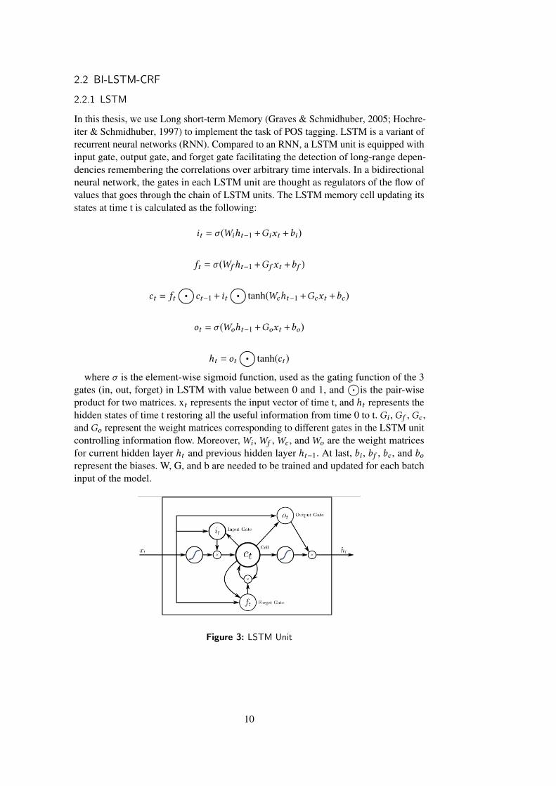
In this thesis, we use Long short-term Memory (Graves & Schmidhuber, 2005; Hochre-iter & Schmidhuber, 1997) to implement the task of POS tagging. LSTM is a variant ofrecurrent neural networks (RNN). Compared to an RNN, a LSTM unit is equipped withinput gate, output gate, and forget gate facilitating the detection of long-range depen-dencies remembering the correlations over arbitrary time intervals. In a bidirectionalneural network, the gates in each LSTM unit are thought as regulators of the flow ofvalues that goes through the chain of LSTM units. The LSTM memory cell updating itsstates at time t is calculated as the following:

it = σ (Wiht−1+Gixt +bi )

ft = σ (Wf ht−1+Gf xt +bf )

ct = ft⊙

ct−1+ it⊙

tanh(Wcht−1+Gcxt +bc )

ot = σ (Woht−1+Goxt +bo)

ht = ot⊙

tanh(ct )where σ is the element-wise sigmoid function, used as the gating function of the 3

gates (in, out, forget) in LSTM with value between 0 and 1, and⊙

is the pair-wiseproduct for two matrices. xt represents the input vector of time t, and ht represents thehidden states of time t restoring all the useful information from time 0 to t. Gi , Gf , Gc ,and Go represent the weight matrices corresponding to different gates in the LSTM unitcontrolling information flow. Moreover,Wi ,Wf ,Wc , andWo are the weight matricesfor current hidden layer ht and previous hidden layer ht−1. At last, bi , bf , bc , and borepresent the biases. W, G, and b are needed to be trained and updated for each batchinput of the model.

Figure 3: LSTM Unit

10

2.2.2 BI-LSTM

For the task of POS, considering both past (Forward LSTM layer in Figure 4) and future(Backward LSTM layer in Figure 4) contexts will be beneficial to the performance.Given a current input feature, its POS tagging is not only influenced by its previousinputs, but also the following inputs after it. This bidirectional – LSTM can efficientlyrestore the past and future information to identify current state (Dyer, Ballesteros,Ling, Matthews, & Smith, 2015). This BI-LSTM can be trained by back-propagationthrough time (BPTT) (Boden, 2002). In each BI-LSTM unit, there are two separatehidden states remembering the past and future information given current input. In eachbatch of training, the hidden states will be updated. Finally, the two hidden states areconcatenated as one output after the training. In our model, the input for BI-LSTM isa concatenated embedding including word, subword, and character representations inwhich the subword and character representations are processed through previous CNNs.Suppose the pre-trained word embedding is Wi = (wi1,wi2,wi3, ...,wil ), the subwordembedding processed by CNNs is Si = (si1,si2, ...,sin), and the character embeddingprocessed by CNNs is Ci = (ci1,ci2, ...,cim) where l, n, and m represent the dimensionof corresponding embedding and i represents the ith word in a sentence. As a result, theconcatenated word representation is Ti = (Wi ,Si ,Ci ), which is the input of BI-LSTM. Inthis model, we set the length of each sentence to a fixed value, which is called maximumtime step. If the maximum time steps is set to 50, it means there are 50 units of BI-LSTM sequentially connected with each other. When the length of a sentence is lessthan 50, the indices will be filled by padding tokens outside of the sentence boundaries.Otherwise, we only process the first 50 words of the sentence. Each BI-LSTM has twoseparate hidden layers: forwards and backwards which are used to capture past andfuture information individually (See Figure 4). The two hidden layers are concatenatedto form the final output. In this model, we set the hidden states = 200 for each LSTM.Because we have two hidden layers: Forward and Backward, the size of the output foreach LSTM is 2×200 = 400 after concatenating. Suppose the forward and backwardhidden states of each BI-LSTM are Fi = (ai1,ai2, ...,aik ) and Bi = (bi1,bi2, ...,bik ) wherek represents the state size of each BI-LSTM unit and i represents the ith BI-LSTM unit.The final output of two concatenated hidden layers for the ith BI-LSTM unit is (Fi ,Bi ) .

2.2.3 CRF

The CRF (Lafferty et al., 2001) is a discriminative model that can capture a largeamount of interacting and dependent features by taking context into account. By usingCRF, we try to optimise the output of sequence labelling over sentence level instead ofindividual positions. Given a sentence, the optimal sequence of labels are determinedby neighbourhoods and grammatical structure of each sentence. As a result, addingCRF can generate higher accuracy rate in general compared with BI-LSTM-CNNmodel(Huang et al., 2015; Ma & Hovy, 2016).

Suppose the compound output from word level BI-LSTM isOi = (oi,1,oi,2,oi,3,...,oi,n)where n represents the LSTM state size and i represents the i th word in a sentence.CRF method states the probability of a sequence POS tags given the BI-LSTM outputover a sentence. This is denoted by p(y |O) where y represents the predicted sequenceof POS tags and O is the BI-LSTM output.

11

Similar to Ma and Hovy (2016), the probability is defined as follows.

p(y | oi ) =∏n

j=1φ(yj−1,yj ,oj )∑y′∈Ω (O )

∏nj=1φ(y ′j−1,y

′j ,oj )

(2.1)

Ω(O) denotes the set of all possible combinations of label sequences,

φ(yj−1,yj ,oj ) = exp(Wyj−1,yjoj +byj−1,yj )where Wyj−1,yj and byj−1,yj represent the weight and bias parameters.We want to minimize the negative log-likelihood in the training process, and update theparameters,W and b.

ζCRF = −∑

loдp(yi |Oi ) (2.2)

At last, after training the parameters,W and b, we use this model to find out the mostlikely sequence y∗ maximising the likelihood.

y∗ = arд maxy∈Ω(O )

p(y |O) (2.3)

The Equation 2 and 3 can be calculated through the Viterbi algorithm.

2.3 BI-LSTM-CNNs-CRF

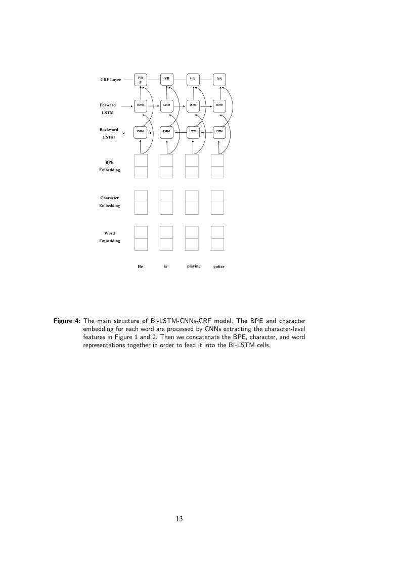
At last, we need to connect the concatenated hidden states of LSTM to CRF layer.Figure 4 shows the structure of our neural network model. First of all, for each inputword, we obtain its character- and subword level representations through CNNs inFigure 1 and 2. The inputs of CNNs are character and subword embeddings padding asthe same length for each word. After the process of CNNs, the character- and subword-level representation vectors are concatenated with the pre-trained word embeddingvector. As a whole, it is fed into BI-LSTM network. Finally, we input the concatenatedhidden states of BI-LSTM to the CRF layer to jointly decode the optimal POS taggingfor an entire sentence.

12

PRP

VB VB NN

LSTM LSTMLSTM LSTM

LSTM LSTMLSTM LSTM

CRF Layer

Forward

LSTM

Backward

LSTM

Word

Embedding

He playing is guitar

Character

Embedding

BPE

Embedding

Figure 4: The main structure of BI-LSTM-CNNs-CRF model. The BPE and characterembedding for each word are processed by CNNs extracting the character-levelfeatures in Figure 1 and 2. Then we concatenate the BPE, character, and wordrepresentations together in order to feed it into the BI-LSTM cells.

13

3 Training for the Neural Network

In this section, we provide details about the hyper-parameters and initial values settingfor this model. This model is implemented by the TensorFlow 1.5.0 library (Abadi etal., 2016). It is trained 30 epochs for each experiment.

3.1 Hyper-Parameters

English Spanish GermanCharacter embedding dimension 300 100 100

Word embedding dimension 100 100 100BPE embedding dimension 100 100 100

Window size 2 2 2LSTM state size 200 200 200

Conv. filter number 50 50 50Optimiser Adagrad Adagrad Adagrad

Initial learning rate 0.05 0.05 0.05Decay rate 0.05 0.05 0.05

Dropout rate 0.5 0.5 0.5Batch size 10 10 10

Maximum time step 50 150 50

Table 1: Hyper-Parameters

Table 1 shows the hyper-parameters setting in our model. The combination of thehyper-parameters are learned and turned from previous successful experiments. Santosand Zadrozny (2014) introduced the method of extracting character- and subword- levelinformation through CNNs, and the CNN’s hyper-parameters was embedded in themodel. LSTM state size, Optimiser, Initial learning rate, Decay rate, Dropout rate, andBatch size were tuned by random search across the space of full hyper-parameters (Ma& Hovy, 2016), so we assigned the same values as theirs. However, we set characterembedding dimension as 100 and Conv. filter number as 50 instead of their choices, 30and 30 respectively. As a result, we try to use 100 dimensional vector and 50 filters tocapture more morphological features in CNNs. The Maximum time step refers to thefixed input length for each sentence in our model. Suppose a character embedding elof dchr dimensions and window size w so the size of convolutional filter in the CNNs,f , is f ∈ R(2×w+1)×dchr . The dimensional size of randomly initialised embeddings forword and character are uniformly set to 100. Moreover, after exploring the corpora ofEnglish, Spanish, and German, I found that for the Spanish datasets there are significantamount of sentences contains more than 50 words so I set the Maximum time step to150 for Spanish which are different from English’s and German’s setting, 50.

14

3.2 Variable Initialisation

3.2.1 Weights and Bias Initialisation

Weight matrices are randomly assigned with uniform distribution over [-x, x], where x

=√

6r+c and r and c represent the number of rows and columns ( Glorot and Bengio ,

2010). Bias is set to zero, except the bias for CNNs, which is set to 0.1.

3.2.2 Embeddings

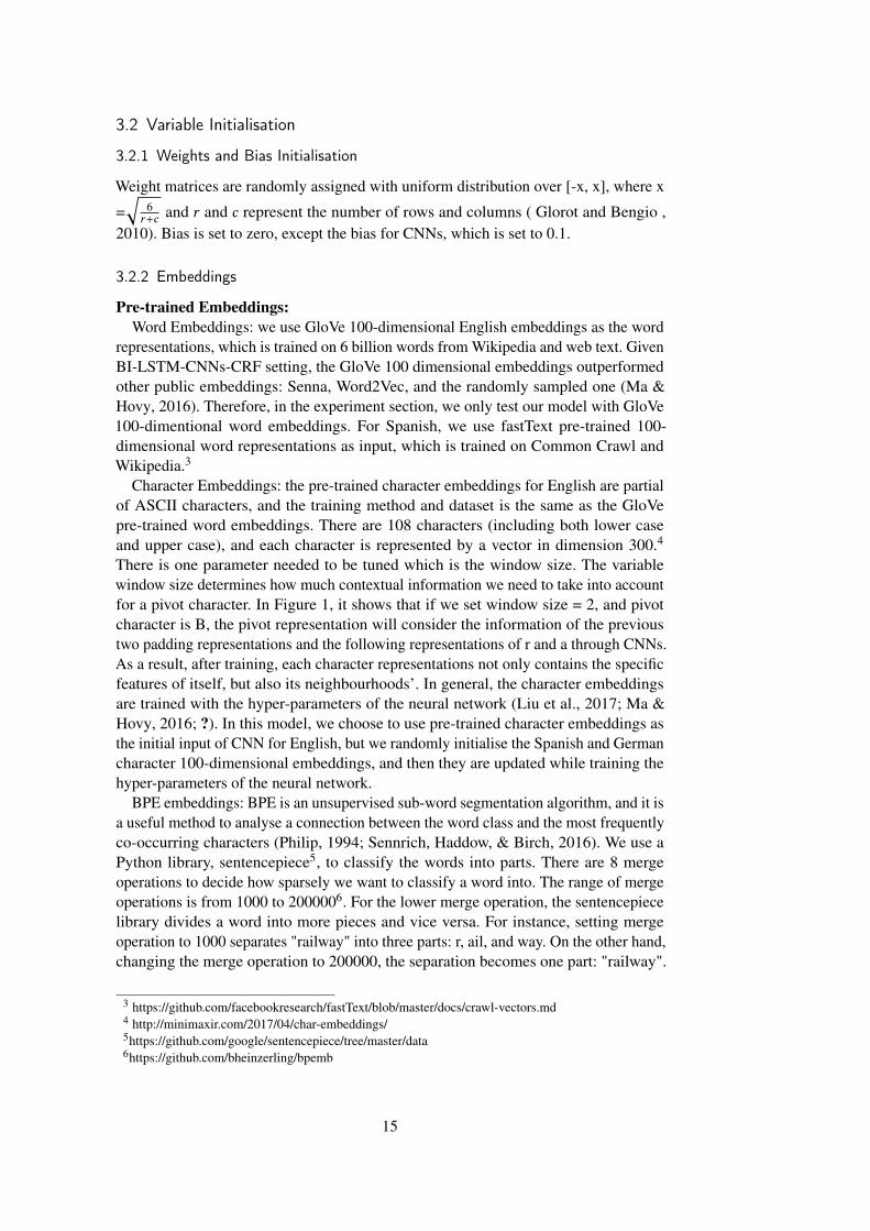
Pre-trained Embeddings:Word Embeddings: we use GloVe 100-dimensional English embeddings as the word

representations, which is trained on 6 billion words from Wikipedia and web text. GivenBI-LSTM-CNNs-CRF setting, the GloVe 100 dimensional embeddings outperformedother public embeddings: Senna, Word2Vec, and the randomly sampled one (Ma &Hovy, 2016). Therefore, in the experiment section, we only test our model with GloVe100-dimentional word embeddings. For Spanish, we use fastText pre-trained 100-dimensional word representations as input, which is trained on Common Crawl andWikipedia.3

Character Embeddings: the pre-trained character embeddings for English are partialof ASCII characters, and the training method and dataset is the same as the GloVepre-trained word embeddings. There are 108 characters (including both lower caseand upper case), and each character is represented by a vector in dimension 300.4

There is one parameter needed to be tuned which is the window size. The variablewindow size determines how much contextual information we need to take into accountfor a pivot character. In Figure 1, it shows that if we set window size = 2, and pivotcharacter is B, the pivot representation will consider the information of the previoustwo padding representations and the following representations of r and a through CNNs.As a result, after training, each character representations not only contains the specificfeatures of itself, but also its neighbourhoods’. In general, the character embeddingsare trained with the hyper-parameters of the neural network (Liu et al., 2017; Ma &Hovy, 2016; ?). In this model, we choose to use pre-trained character embeddings asthe initial input of CNN for English, but we randomly initialise the Spanish and Germancharacter 100-dimensional embeddings, and then they are updated while training thehyper-parameters of the neural network.

BPE embeddings: BPE is an unsupervised sub-word segmentation algorithm, and it isa useful method to analyse a connection between the word class and the most frequentlyco-occurring characters (Philip, 1994; Sennrich, Haddow, & Birch, 2016). We use aPython library, sentencepiece5, to classify the words into parts. There are 8 mergeoperations to decide how sparsely we want to classify a word into. The range of mergeoperations is from 1000 to 2000006. For the lower merge operation, the sentencepiecelibrary divides a word into more pieces and vice versa. For instance, setting mergeoperation to 1000 separates "railway" into three parts: r, ail, and way. On the other hand,changing the merge operation to 200000, the separation becomes one part: "railway".

3 https://github.com/facebookresearch/fastText/blob/master/docs/crawl-vectors.md4 http://minimaxir.com/2017/04/char-embeddings/5https://github.com/google/sentencepiece/tree/master/data6https://github.com/bheinzerling/bpemb

15

Therefore, we need to find out the optimal combination of the merge operation andwindow size as a whole to deliver the best performance. Moreover, the byte pairs arepresented by real numbers in the Python library, sentencepiece; therefore, we need toincorporate it with another Python library, KeyedVectors7, to extract the pre-trained100-dimensional BPE embeddings for the corresponding byte pairs before feeding theminto CNNs.Randomly Initialised Embeddings:

Word Embeddings: For German, we can not use pre-trained word embeddings be-cause the size of embeddings is as large as 5.97G, which can not be processed by ourlimited memory, 32G, exceeding the limit of our memory before training. Therefore,we randomly initialise all the German word embeddings as 100-dimensional vectors

where embeddings are uniformly sampled over [-x, x], where x =√

3dim where dim is

the dimension of embeddings (Ma & Hovy, 2016).Character Embeddings: German and Spanish character embeddings are initialised

over uniform distribution [-x, x], where x =√

3dim where we set dim = 100.

Embeddings English Spanish GermanWord Pre-trained GloVe Pre-trained fastText Randomly Initialised

Character Pre-trained 300-dim Randomly Initialised Randomly InitialisedBPE Pre-trained 100-dim Pre-trained 100-dim Pre-trained 100-dim

Table 2: The inputs of the neural network models.

Table 2 indicates the inputs of the neural network models for different languages inthis thesis. For English, we choose pre-trained 100-dimensional GloVe word embed-dings and 300-dimensional GloVe character embeddings as the inputs. For Spanish, wechoose pre-trained 100-dimensional fastText word embeddings and randomly initialised100-dimensional character embeddings as the inputs. For German, we choose to feedword and character embeddings with randomly initialised 100-dimensional embeddingsfor the neural network models. As shown in Table 2, all BPE embeddings are pre-trained100-dimensional embeddings (Heinzerling & Strube, 2017). Because we only comparethe different neural network models’ performances with the same inputs for a specificlanguage, the variation of the inputs for different languages will not influence ouranalysis and comparison.

3.3 Optimization for Loss

Adagrad (Duchi, Hazan, & Singer, 2011) is used to minimize the loss with initiallearning rate 0.05 updating with decay rate ϱt=0.05 as training epoch t increases,ηt =η0ϱt+1 where η0 = 0.05 is initial learning rate.

3.4 Dropout Training

In order to avoid overfitting, we implement dropout regularisation to the output ofBI-LSTM layer with a fix value of 0.5 (Srivastava, Hinton, Krizhevsky, Sutskever, &Salakhutdinov, 2014).

7https://github.com/bheinzerling/bpemb

16

SET SENT. TOKENS OOTV OOBVTraining 12250 167915 0 0

Dev. 1965 21312 4931 0Test 2052 21102 5186 2061

Table 3: UD Corpus for English POS.


Dev. 1654 46263 8348 0Test 1721 46531 2937 2786

Table 4: UD Corpus for Spanish POS.

4 Experiments

4.1 Datasets

For the POS tagging task, we use Universal Dependencies (UD) datasets of English,Spanish, and German, which includes 17, 18, 16 POS tags according to its kind. Thedataset for each language is classified into three parts: training, development, and test.In Table 3, 4, and 5, it shows the details of the UD corpus. The column OOTV showsthe number of out-of-the-training-vocabulary words (OOTV) in development dataset ortest dataset. The last column OOBV shows the number of out-of-the-training and dev-vocabulary (OOBV) words in testing dataset.

4.2 Main Results

First of all, we test the possible combinations of window size and BPE merge operationsfor our model on English given other hyper-parameters unchanged. Table 6 showsthat setting window size of 2 and BPE of 10000 obtains better performance than othersettings. As our previous explanation, when the window size is small, it implies weconsider less contextual information at character level. On the other hand, if we set BPEat a small merge operation, it sparsely separates a word into pieces providing the samefunction as character embedding. In order to extract all the morphological informationefficiently, our best setting should have small window size and medium BPE becauseif we set BPE at a large value, its function will be similar to word embedding. As a


Dev. 799 11013 4563 0Test 972 14219 1922 1836

Table 5: UD Corpus for German POS.

17

BPE: 3000 BPE: 5000 BPE:10000 BPE:25000 BPE:50000Window Size ACC. ACC. ACC. ACC. ACC.

1 0.949893 0.949314 0.950843 0.950265 0.9500582 0.950595 0.949479 0.951050 0.949934 0.9498513 0.949272 0.948735 0.948073 0.950430 0.9491484 0.949148 0.949396 0.950430 0.948611 0.9482805 0.949810 0.949934 0.949396 0.950099 0.947908

Table 6: BI-LSTM-CNNs-CRF-BPE on the Dev dataset for English.

Dev TestACC. ACC.

BI-LSTM (without character embedding) 0.9118 0.9138BI-LSTM-CNNs 0.9433 0.9473

BI-LSTM-CNNs-CRF 0.9471 0.9501BI-LSTM-CNNs-CRF-BPE 0.9485 0.9513

Table 7: Results of different neural network models with identical inputs.

whole, we try to extract the useful information from different perspectives in our model:character-level, subword-level, and word-level. At last, the output interface, CRF, willconsider all the information at sentence-level to optimise the sequence labelling.

We compare our model with other systems: BI-LSTM, BI-LSTM-CNNs, and BI-LSTM-CNNs-CRF. Table 7 shows that BI-LSTM’s performance is lower than othermodels’ by at least 3.2 percentage points on both dev and test datasets . This implies thatthe character embeddings plays an important role for POS tagging. Moreover, the CRFcan improve the accuracy by 0.6 percentage points and 0.3 percentage points on devand test datasets respectively. Our model, BI-LSTM-CNNs-CRF-BPE, delivers the bestperformance, 95.1050 percentage points and 95.0664 percentage points respectively.However, the differences of performance between BI-LSTM-CNNs-CRF-BPE andBI-LSTM-CNNs-CRF is not obvious. After implementing null hypothesis significancetesting we find out that for the testing dataset the p-value is 0.7538 so this result wouldbe deemed not statistically significant and, the hypothesis that the model with BPEhas the same performance as the one without BPE’s would not be rejected given asignificance level of 0.05.8 Moreover, for the development dataset, the p-value is 0.5549so it is not statistically significant to reject the hypothesis as well. To sum up, BI-LSTM-CNNs models significantly outperform the BI-LSTM model. By adding CRFand BPE, our model obtains improvements over BI-LSTM-CNNs so jointly decodingand extracting information at subword-level can largely benefit the accuracy of POStagging for English. However, the improvement of BI-LSTM-CNNs-CRF-BPE overBI-LSTM-CNNs-CRF is not statistically significant for development and test datasets.

For English, we obtain a slight improvement by adding BPE on BI-LSTM-CNNs-CRF architecture, which is not statistically significant so we try to experiment two moremorphological languages: Spanish and German. For Spanish, the overall performanceon development and test datasets are much higher than English’s. Table 8 shows thatthe gap between the two different architectures becomes larger than English’s as well,

8https://en.wikipedia.org/wiki/Student%27s_t-test#Independent_two-sample_t-test

18

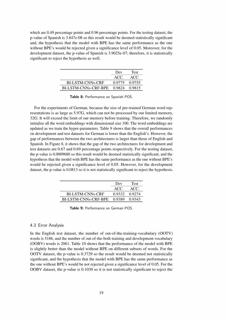
which are 0.49 percentage points and 0.96 percentage points. For the testing dataset, thep-value of Spanish is 3.847e-08 so this result would be deemed statistically significantand, the hypothesis that the model with BPE has the same performance as the onewithout BPE’s would be rejected given a significance level of 0.05. Moreover, for thedevelopment dataset, the p-value of Spanish is 3.9025e-07; therefore, it is statisticallysignificant to reject the hypothesis as well.

Dev TestACC. ACC.


Table 8: Performance on Spanish POS.

For the experiments of German, because the size of pre-trained German word rep-resentations is as large as 5.97G, which can not be processed by our limited memory,32G. It will exceed the limit of our memory before training. Therefore, we randomlyinitialise all the word embeddings with dimensional size 100. The word embeddings areupdated as we train the hyper-parameters. Table 9 shows that the overall performanceson development and test datasets for German is lower than the English’s. However, thegap of performances between the two architectures is larger than those of English andSpanish. In Figure 8, it shows that the gap of the two architectures for development andtest datasets are 0.67 and 0.69 percentage points respectively. For the testing dataset,the p-value is 0.0009680 so this result would be deemed statistically significant, and thehypothesis that the model with BPE has the same performance as the one without BPE’swould be rejected given a significance level of 0.05. However, for the developmentdataset, the p-value is 0.0813 so it is not statistically significant to reject the hypothesis.

Dev TestACC. ACC.


Table 9: Performance on German POS.

4.3 Error Analysis

In the English test dataset, the number of out-of-the-training-vocabulary (OOTV)words is 5186, and the number of out-of-the-both training and development-vocabulary(OOBV) words is 2061. Table 10 shows that the performance of the model with BPEis slightly better than the model without BPE on different subsets of words. For theOOTV dataset, the p-value is 0.3729 so the result would be deemed not statisticallysignificant, and the hypothesis that the model with BPE has the same performance asthe one without BPE’s would be not rejected given a significance level of 0.05. For theOOBV dataset, the p-value is 0.1030 so it is not statistically significant to reject the

19

hypothesis. To sum up, the improvements on different out-of-vocabulary subsets arenot statistically significant for English POS tagging.

Testing DatasetOOTV OOBV


Table 10: Comparison of performance on different out-of-vocabulary subsets of words(accuracy for POS).

Figure 5 and 6 show that the BPE model is good at tagging the PROPN and VERB onthe corresponding English subsets, and the model without BPE has better performanceon ADJ and NOUN. For instance, the performance of the model with BPE achieved 643correct tags of the PROPN on OOTV dataset; on the other hand, the one without BPEonly obtained 618 correct tags on PROPN. Meanwhile, the model without BPE obtained142 and 586 correct tags on the ADJ and NOUN respectively which are more than theBPE model’s 134 and 560. According to the confusion matrices, we can conclude thatboth the model with and without BPE have some space to be improved for taggingPROPN and NOUN because most of errors occurred on these two tags. In addition, thereis a significant number of ADJ was incorrectly tagged as NOUN, PROPN, and VERB.For example, in Figure 7, it shows that there are 28, 8, and 7 ADJ were incorrectlytagged as NOUN, PROPN, and VERB respectively in the model with BPE; meanwhile,there are 20, 6, and 7 ADJ were incorrectly tagged in the one without BPE. Based onthe error analysis, we found that the model would obtain better performance if we candistinguish the PROPN and NOUN more efficiently.

Table 11 shows that the model with BPE outperforms the one without BPE on bothOOTV and OOBV for Spanish testing dataset. The model with BPE improves theaccuracy by 1.7 for OOTV and 1.62 for OOBV. The confusion matrix in Figure 7 showsthe details of performances of Spanish POS tagging on OOTV. In general, PROPN,NOUN, VERB, and ADJ account for the majority of the out-of-vocabulary words forSpanish datasets. When we look at the diagonals of the two tables, the number of correctlabel on corresponding tags, the model with BPE outperforms the one without BPE onall kinds of tags. According to both of the confusion matrices, we can conclude thatboth of the models have the worst performances on distinguishing NOUN from ADJ,PROPN, and VERB. For the model with BPE, it mislabeled 28, 24, and 10 NOUN asADJ, PROPN, and VERB respectively. Meanwhile, the model without BPE obtainedslightly worse performance: mislabelling 35, 30, and 8 NOUN as ADJ, PROPN, andVERB respectively. Moreover, the two models mislabeled 63 and 62 ADJ as NOUNwhich are the worst performance in frequency and proportion of errors. In Figure 8, itshows the confusion matrices of OOBV for Spanish testing dataset, and they have thesame patterns as OOTV’s. Therefore, the model with BPE obtains better performanceson Spanish out-of-vocabulary datasets. The two architectures mislabeled some NOUNas ADJ, PROPN, and VERB, but the biggest challenge of the architectures on Spanishdatasets is distinguishing ADJ and NOUN. For the OOTV dataset, the p-value is 6.977e-08 so this result would be deemed statistically significant, and the hypothesis that themodel with BPE has the same performance as the one without BPE’s would be rejected

20

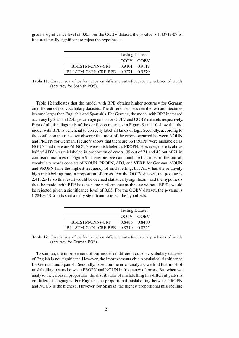
given a significance level of 0.05. For the OOBV dataset, the p-value is 1.4371e-07 soit is statistically significant to reject the hypothesis.



Table 11: Comparison of performance on different out-of-vocabulary subsets of words(accuracy for Spanish POS).

Table 12 indicates that the model with BPE obtains higher accuracy for Germanon different out-of-vocabulary datasets. The differences between the two architecturesbecome larger than English’s and Spanish’s. For German, the model with BPE increasedaccuracy by 2.24 and 2.45 percentage points for OOTV and OOBV datasets respectively.First of all, the diagonals of the confusion matrices in Figure 9 and 10 show that themodel with BPE is beneficial to correctly label all kinds of tags. Secondly, according tothe confusion matrices, we observe that most of the errors occurred between NOUNand PROPN for German. Figure 9 shows that there are 36 PROPN were mislabeled asNOUN, and there are 61 NOUN were mislabeled as PROPN. However, there is abovehalf of ADV was mislabeled in proportion of errors, 39 out of 71 and 43 out of 71 inconfusion matrices of Figure 9. Therefore, we can conclude that most of the out-of-vocabulary words consists of NOUN, PROPN, ADJ, and VERB for German. NOUNand PROPN have the highest frequency of mislabelling, but ADV has the relativelyhigh mislabelling rate in proportion of errors. For the OOTV dataset, the p-value is2.4152e-17 so this result would be deemed statistically significant, and the hypothesisthat the model with BPE has the same performance as the one without BPE’s wouldbe rejected given a significance level of 0.05. For the OOBV dataset, the p-value is1.2849e-19 so it is statistically significant to reject the hypothesis.



Table 12: Comparison of performance on different out-of-vocabulary subsets of words(accuracy for German POS).

To sum up, the improvement of our model on different out-of-vocabulary datasetsof English is not significant. However, the improvements obtain statistical significancefor German and Spanish. Secondly, based on the error analysis, we find that most ofmislabelling occurs between PROPN and NOUN in frequency of errors. But when weanalyse the errors in proportion, the distribution of mislabelling has different patternson different languages. For English, the proportional mislabelling between PROPNand NOUN is the highest . However, for Spanish, the highest proportional mislabelling

21

occurs between NOUN and ADJ. For German, the highest proportional mislabelling isbetween ADJ and ADV.

4.4 Related Work

Our system is built upon the achievement of LSTM-CNNs-CRF model and is furtherimproved to better capture the relationship between POS tagging and subword structuresthrough BPE embedding. The best accuracy of BI-LSTM-CNNs-CRF (Ma & Hovy,2016) is as high as 97.55% for POS tagging, and the best accuracy of LM-LSTM-CRF framework (Liu et al., 2017) achieves 97.59% for POS tagging. One importantreason that based on the same neural network architectures their accuracy is higherthan ours is their models implement larger training, development, and testing datasets.Their POS datasets are from the Wall Street Journal (WSJ) portion of Penn Treebank(PTB) containing 38219 sentences for training, 5527 sentences for development, and5462 sentences for test. However, we implement UD datasets to experiment our modelwhich contains 12250 sentences for training, 1965 sentences for development, and 2052sentences for test. Because we have limited computational power to run the experiments,in order to test and compare different hyper-parameter settings and languages, we haveto shrink our datasets. Moreover, the main goal of this thesis is to verify if the BPEembedding can improve the accuracy of POS tagging task based on BI-LSTM-CNNs-CRF architectures. Therefore, when we use the same datasets to test the different neuralnetwork architectures, the comparisons are statistically reliable as long as the datasetsare sufficiently large.

22

5 Conclusion and Further Work

In this thesis, we jointly use word-level, subword-level, and character-level represen-tations to perform English, Spanish, and German POS tagging tasks based on thefundamental neural network architecture: BI-LSTM-CNNs-CRF. The main contributionincludes (1) proposing an end-to-end system using CNNs to leverage the character-and subword- level knowledges collaborating with word-level features, (2) finding outthe pattern of optimal combination of window size and BPE merge operations whichachieves improvement over other baseline systems, (3) improving the accuracy of POStagging on more morphological languages such as Spanish and German than English,(4) through testing the out-of-vocabulary subsets, we found that our model obtainsstatistical significance improvement on more morphological languages which is notobserved on English. (5) based on the error analysis, we found that there are differentmislabelling patterns for different languages. There are two interesting part can befurther developed. First of all, tuning the best combination of window size and BPEmerge operation will be crucial for different morphological languages because these twoparameters contribute a significant effect to the results. Secondly, it would be interestingto analyse the errors with detailed examples for German and Spanish.

23

Figure 5: Confusion Matrix of OOTV for the English testing dataset. The upper table isthe confusion matrix of BI-LSTM-CNNs-CRF-BPE, and the lower table is theconfusion matrix of BI-LSTM-CNNs-CRF. The column names represent the realtags and the rows represent predicted ones.

24

Figure 6: Confusion Matrix of OOBV for English testing dataset. The upper table isthe confusion matrix of BI-LSTM-CNNs-CRF-BPE, and the lower table is theconfusion matrix of BI-LSTM-CNNs-CRF. The column names represent the realtags and the rows represent predicted ones.

25

Figure 7: Confusion Matrix of OOTV for Spanish testing dataset. The upper table isthe confusion matrix of BI-LSTM-CNNs-CRF-BPE, and the lower table is theconfusion matrix of BI-LSTM-CNNs-CRF. The column names represent the realtags and the rows represent predicted ones.

26

Figure 8: Confusion Matrix of OOBV for Spanish testing dataset.The upper table is theconfusion matrix of BI-LSTM-CNNs-CRF-BPE, and the lower table is the confu-sion matrix of BI-LSTM-CNNs-CRF. The column names represent the real tagsand the rows represent predicted ones.

27

Figure 9: Confusion Matrix of OOTV for German testing dataset. The upper table isthe confusion matrix of BI-LSTM-CNNs-CRF-BPE, and the lower table is theconfusion matrix of BI-LSTM-CNNs-CRF. The column names represent the realtags and the rows represent predicted ones.

28

Figure 10: Confusion Matrix of OOBV for German testing dataset. The upper table isthe confusion matrix of BI-LSTM-CNNs-CRF-BPE, and the lower table is theconfusion matrix of BI-LSTM-CNNs-CRF. The column names represent the realtags and the rows represent predicted ones.

29

References

Abadi, M., Barham, P., Chen, J., Chen, Z., Davis, A., Dean, J., . . . others (2016).Tensorflow: a system for large-scale machine learning. In Osdi (Vol. 16, pp.265–283).

Boden, M. (2002). A guide to recurrent neural networks and backpropagation. theDallas project.

Chen, D., & Manning, C. (2014). A Fast and Accurate Dependency Parser usingNeural Networks. Proceedings of the 2014 Conference on Empirical Methods inNatural Language Processing (EMNLP)(i), 740–750. Retrieved from http://aclweb.org/anthology/D14-1082 doi: 10.3115/v1/D14-1082

Chiu, J. P., & Nichols, E. (2015). Named entity recognition with bidirectional lstm-cnns.arXiv preprint arXiv:1511.08308.

Collobert, R., Weston, J., Bottou, L., Karlen, M., Kavukcuoglu, K., & Kuksa, P. (2011).Natural language processing (almost) from scratch. Journal of Machine LearningResearch, 12(Aug), 2493–2537.

Duchi, J., Hazan, E., & Singer, Y. (2011). Adaptive subgradient methods for onlinelearning and stochastic optimization. Journal of Machine Learning Research,12(Jul), 2121–2159.

Dyer, C., Ballesteros, M., Ling, W., Matthews, A., & Smith, N. A. (2015). Transition-based dependency parsing with stack long short-term memory. arXiv preprintarXiv:1505.08075.

Graves, A., & Schmidhuber, J. (2005). Framewise phoneme classification with bidi-rectional lstm and other neural network architectures. Neural Networks, 18(5-6),602–610.

Heinzerling, B., & Strube, M. (2017). Bpemb: Tokenization-free pre-trained subwordembeddings in 275 languages. arXiv preprint arXiv:1710.02187.

Hochreiter, S., & Schmidhuber, J. (1997). Long short-term memory. Neural computa-tion, 9(8), 1735–1780.

Huang, Z., Xu, W., & Yu, K. (2015). Bidirectional lstm-crf models for sequence tagging.2015. arxiv preprint. arXiv preprint arXiv:1508.01991.

Koo, T., & Collins, M. (2010). Efficient third-order dependency parsers. Proceedingsof the 48th Annual Meeting of the Association for Computational Linguistics(ACL ’10)(July), 1–11.

Lafferty, J., McCallum, A., & Pereira, F. C. (2001). Conditional random fields:Probabilistic models for segmenting and labeling sequence data. In Proceedingsof ICML-2001, 951, 282–289.

Le Cun, Y., Jackel, L., Boser, B., Denker, J., Graf, H., Guyon, I., . . . Hubbard, W.(1989). Handwritten digit recognition: Applications of neural network chips andautomatic learning. IEEE Communications Magazine, 27(11), 41–46.

Liu, L., Shang, J., Xu, F., Ren, X., Gui, H., Peng, J., & Han, J. (2017). Em-power sequence labeling with task-aware neural language model. arXiv preprintarXiv:1709.04109.

30

http://aclweb.org/anthology/D14-1082

http://aclweb.org/anthology/D14-1082

Luo, G., Huang, X., Lin, C.-Y., & Nie, Z. (2015). Joint entity recognition and dis-ambiguation. In Proceedings of the 2015 conference on empirical methods innatural language processing (pp. 879–888).

Ma, X., & Hovy, E. (2016). End-to-end sequence labeling via bi-directional lstm-cnns-crf. arXiv preprint arXiv:1603.01354.

Ma, X., & Zhao, H. (2012). Fourth-order dependency parsing. Proceedings of COLING2012: posters, 785–796.

Ma, X., & Zhao, H. (2015). Probabilistic models for high-order projective dependencyparsing. arXiv preprint arXiv:1502.04174.

McCallum, A., Freitag, D., & Pereira, F. C. (2000). Maximum entropy markov modelsfor information extraction and segmentation. In Proceedings of ICML-2000,591–598.

McDonald, R., Crammer, K., & Pereira, F. (2005). Online large-margin training ofdependency parsers. In Proceedings of the 43rd annual meeting on associationfor computational linguistics (pp. 91–98).

Nivre, J., & Scholz, M. (2004). Deterministic dependency parsing of english text. InProceedings of the 20th international conference on computational linguistics(p. 64).

Passos, A., Kumar, V., & McCallum, A. (2014). Lexicon infused phrase embeddingsfor named entity resolution. arXiv preprint arXiv:1404.5367.

Pennington, J., Socher, R., & Manning, C. (2014). Glove: Global vectors for wordrepresentation. In Proceedings of the 2014 conference on empirical methods innatural language processing (pp. 1532–1543).

Philip, G. (1994). A New Algorithm for Data Compression. The C Users Journal, 12Issue 2, 23 - 38.

Ratinov, L., & Roth, D. (2009). Design challenges and misconceptions in namedentity recognition. In Proceedings of the thirteenth conference on computationalnatural language learning (pp. 147–155).

Santos, C. D., & Zadrozny, B. (2014). Learning character-level representations forpart-of-speech tagging. In Proceedings of the 31st international conference onmachine learning (icml-14) (pp. 1818–1826).

Sennrich, R., Haddow, B., & Birch, A. (2016). Edinburgh neural machine translationsystems for wmt 16. arXiv preprint arXiv:1606.02891.

Srivastava, N., Hinton, G., Krizhevsky, A., Sutskever, I., & Salakhutdinov, R. (2014).Dropout: a simple way to prevent neural networks from overfitting. The Journalof Machine Learning Research, 15(1), 1929–1958.

Turian, J., Ratinov, L., & Bengio, Y. (2010). Word representations: a simple and generalmethod for semi-supervised learning. In Proceedings of the 48th annual meetingof the association for computational linguistics (pp. 384–394).

31

bidirectional lstm-cnns-crf models for pos...

Documents