The University of Manchester Research

Bifurcation and stability of elastic membranes: theory andbiological applications

Link to publication record in Manchester Research Explorer

Citation for published version (APA):Pearce, S. (2010). Bifurcation and stability of elastic membranes: theory and biological applications. University ofKeele.

Citing this paperPlease note that where the full-text provided on Manchester Research Explorer is the Author Accepted Manuscriptor Proof version this may differ from the final Published version. If citing, it is advised that you check and use thepublisher's definitive version.

General rightsCopyright and moral rights for the publications made accessible in the Research Explorer are retained by theauthors and/or other copyright owners and it is a condition of accessing publications that users recognise andabide by the legal requirements associated with these rights.

Takedown policyIf you believe that this document breaches copyright please refer to the University of Manchester’s TakedownProcedures [http://man.ac.uk/04Y6Bo] or contact uml.scholarlycommunications@manchester.ac.uk providingrelevant details, so we can investigate your claim.

Download date:26. Feb. 2022

Bifurcation and stability of elastic membranes:

theory and biological applications

S. P. Pearce

PhD Thesis

February 2010

Keele University

Contents

1 Introduction 1

1.1 Introduction . . . . . . . . . . . . . . . . . . . . . . . . . . . . . . . . . . . . 1

2 Mathematical Preliminaries 6

2.1 Continuum Mechanics . . . . . . . . . . . . . . . . . . . . . . . . . . . . . . 6

2.1.1 Introduction . . . . . . . . . . . . . . . . . . . . . . . . . . . . . . . . 6

2.1.2 Bodies and Configurations . . . . . . . . . . . . . . . . . . . . . . . 6

2.1.3 Tensor Algebra . . . . . . . . . . . . . . . . . . . . . . . . . . . . . . 7

2.1.4 Deformation Gradient . . . . . . . . . . . . . . . . . . . . . . . . . . 10

2.1.5 Conservation of mass . . . . . . . . . . . . . . . . . . . . . . . . . . 13

2.1.6 Conservation of Momentum . . . . . . . . . . . . . . . . . . . . . . 14

2.1.7 Equations of Motion . . . . . . . . . . . . . . . . . . . . . . . . . . . 15

2.1.8 Constitutive Models . . . . . . . . . . . . . . . . . . . . . . . . . . . 16

2.1.9 Elasticity . . . . . . . . . . . . . . . . . . . . . . . . . . . . . . . . . . 18

2.1.10 Isotropy . . . . . . . . . . . . . . . . . . . . . . . . . . . . . . . . . . 19

2.1.11 Conservation of Energy . . . . . . . . . . . . . . . . . . . . . . . . . 20

2.2 Strain-Energy Functions . . . . . . . . . . . . . . . . . . . . . . . . . . . . . 21

2.2.1 Varga Strain-Energy Function . . . . . . . . . . . . . . . . . . . . . . 23

2.2.2 Neo-Hookean Strain-Energy Function . . . . . . . . . . . . . . . . . 24

2.2.3 Mooney-Rivlin Strain-Energy Function . . . . . . . . . . . . . . . . 24

2.2.4 Gent Strain-Energy Function . . . . . . . . . . . . . . . . . . . . . . 24

2.2.5 General Separable Strain-Energy Function . . . . . . . . . . . . . . 25

i

2.2.6 Fung Strain-Energy Function . . . . . . . . . . . . . . . . . . . . . . 26

2.3 Membrane Elasticity . . . . . . . . . . . . . . . . . . . . . . . . . . . . . . . 26

2.3.1 Membrane-Like Shells . . . . . . . . . . . . . . . . . . . . . . . . . . 27

2.3.2 Simple Membranes . . . . . . . . . . . . . . . . . . . . . . . . . . . . 27

2.3.3 Generalised Membranes . . . . . . . . . . . . . . . . . . . . . . . . . 28

2.3.4 Wrinkling . . . . . . . . . . . . . . . . . . . . . . . . . . . . . . . . . 28

2.4 Linear Elasticity . . . . . . . . . . . . . . . . . . . . . . . . . . . . . . . . . . 29

2.4.1 Introduction . . . . . . . . . . . . . . . . . . . . . . . . . . . . . . . . 29

2.4.2 Linearisation . . . . . . . . . . . . . . . . . . . . . . . . . . . . . . . 29

2.4.3 Hooke’s Law . . . . . . . . . . . . . . . . . . . . . . . . . . . . . . . 30

2.4.4 Equilibrium equations . . . . . . . . . . . . . . . . . . . . . . . . . . 33

2.5 Compound Matrix Method . . . . . . . . . . . . . . . . . . . . . . . . . . . 34

2.5.1 Introduction . . . . . . . . . . . . . . . . . . . . . . . . . . . . . . . . 34

2.5.2 Determinant Based Method . . . . . . . . . . . . . . . . . . . . . . . 35

2.5.3 Compound Matrix Method . . . . . . . . . . . . . . . . . . . . . . . 37

2.6 Legendre Functions and Spherical Harmonics . . . . . . . . . . . . . . . . 40

2.6.1 Introduction . . . . . . . . . . . . . . . . . . . . . . . . . . . . . . . . 40

2.6.2 Spherical Harmonics . . . . . . . . . . . . . . . . . . . . . . . . . . . 40

2.6.3 Legendre Polynomials . . . . . . . . . . . . . . . . . . . . . . . . . . 41

2.6.4 Orthogonality and Integral Formulae . . . . . . . . . . . . . . . . . 43

2.6.5 Function Expansion Theorem . . . . . . . . . . . . . . . . . . . . . . 44

2.6.6 Associated Legendre Functions . . . . . . . . . . . . . . . . . . . . . 45

3 Non-Uniform Inflation of a Cylindrical Membrane 47

3.1 Introduction . . . . . . . . . . . . . . . . . . . . . . . . . . . . . . . . . . . . 47

3.2 Literature Review . . . . . . . . . . . . . . . . . . . . . . . . . . . . . . . . . 48

3.2.1 Experimental Studies . . . . . . . . . . . . . . . . . . . . . . . . . . . 48

3.2.2 Analytical Studies . . . . . . . . . . . . . . . . . . . . . . . . . . . . 50

3.3 Inflation of a Cylindrical Tube . . . . . . . . . . . . . . . . . . . . . . . . . . 52

3.3.1 Governing Equations . . . . . . . . . . . . . . . . . . . . . . . . . . . 52

ii

3.3.2 Conditions at Infinity . . . . . . . . . . . . . . . . . . . . . . . . . . 57

3.3.3 Bifurcation Condition . . . . . . . . . . . . . . . . . . . . . . . . . . 60

3.3.4 Connection with the Pressure-Volume Curve . . . . . . . . . . . . . 62

3.4 Localised Solutions . . . . . . . . . . . . . . . . . . . . . . . . . . . . . . . . 64

3.4.1 Near-Critical Solutions . . . . . . . . . . . . . . . . . . . . . . . . . . 66

3.4.2 Phase Plane Analysis . . . . . . . . . . . . . . . . . . . . . . . . . . . 68

3.5 Amplitude-Stretch Diagrams . . . . . . . . . . . . . . . . . . . . . . . . . . 69

3.6 Kinked Solution . . . . . . . . . . . . . . . . . . . . . . . . . . . . . . . . . . 72

3.7 Numerical Solutions . . . . . . . . . . . . . . . . . . . . . . . . . . . . . . . 75

3.8 Conclusion . . . . . . . . . . . . . . . . . . . . . . . . . . . . . . . . . . . . . 77

4 Stability of a Bifurcated Cylindrical Membrane 80

4.1 Introduction . . . . . . . . . . . . . . . . . . . . . . . . . . . . . . . . . . . . 80

4.2 Stability of the Uniform State . . . . . . . . . . . . . . . . . . . . . . . . . . 81

4.3 Stability of the Weakly-Nonlinear Solution . . . . . . . . . . . . . . . . . . 82

4.3.1 Evolution Equation . . . . . . . . . . . . . . . . . . . . . . . . . . . . 83

4.3.2 Compound Matrix Method . . . . . . . . . . . . . . . . . . . . . . . 87

4.3.3 Results . . . . . . . . . . . . . . . . . . . . . . . . . . . . . . . . . . . 89

4.4 Stability of the General Bifurcated State . . . . . . . . . . . . . . . . . . . . 91

4.4.1 Introduction . . . . . . . . . . . . . . . . . . . . . . . . . . . . . . . . 91

4.4.2 Governing Equations . . . . . . . . . . . . . . . . . . . . . . . . . . . 92

4.4.3 Compound Matrix Method . . . . . . . . . . . . . . . . . . . . . . . 93

4.4.4 Results . . . . . . . . . . . . . . . . . . . . . . . . . . . . . . . . . . . 94

4.5 Energy Minimisation . . . . . . . . . . . . . . . . . . . . . . . . . . . . . . . 95

4.6 Conclusion . . . . . . . . . . . . . . . . . . . . . . . . . . . . . . . . . . . . . 100

5 Comparison of Strain-Energy Functions 101

5.1 Introduction . . . . . . . . . . . . . . . . . . . . . . . . . . . . . . . . . . . . 101

5.2 Varga Strain-Energy Function . . . . . . . . . . . . . . . . . . . . . . . . . . 101

5.2.1 Bifurcation Condition . . . . . . . . . . . . . . . . . . . . . . . . . . 101

iii

5.2.2 Amplitude-Stretch Diagram . . . . . . . . . . . . . . . . . . . . . . . 103

5.2.3 Stability . . . . . . . . . . . . . . . . . . . . . . . . . . . . . . . . . . 105

5.3 Neo-Hookean Strain-Energy Function . . . . . . . . . . . . . . . . . . . . . 105

5.3.1 Bifurcation Condition . . . . . . . . . . . . . . . . . . . . . . . . . . 105

5.3.2 Amplitude-Stretch Diagram . . . . . . . . . . . . . . . . . . . . . . . 106

5.4 Gent Strain-Energy Function . . . . . . . . . . . . . . . . . . . . . . . . . . . 107

5.4.1 Bifurcation Condition . . . . . . . . . . . . . . . . . . . . . . . . . . 107

5.4.2 Amplitude-Stretch Diagram . . . . . . . . . . . . . . . . . . . . . . . 108

5.4.3 Stability . . . . . . . . . . . . . . . . . . . . . . . . . . . . . . . . . . 109

5.5 Ogden Strain-Energy Function . . . . . . . . . . . . . . . . . . . . . . . . . 110

5.5.1 Amplitude-Stretch Diagrams . . . . . . . . . . . . . . . . . . . . . . 110

5.5.2 Stability . . . . . . . . . . . . . . . . . . . . . . . . . . . . . . . . . . 113

5.6 Fung Strain-Energy Function . . . . . . . . . . . . . . . . . . . . . . . . . . 113

5.7 Artery Modelling . . . . . . . . . . . . . . . . . . . . . . . . . . . . . . . . . 114

5.8 Conclusion . . . . . . . . . . . . . . . . . . . . . . . . . . . . . . . . . . . . . 115

6 Inflation of a Spherical Membrane 116

6.1 Introduction . . . . . . . . . . . . . . . . . . . . . . . . . . . . . . . . . . . . 116

6.2 Configuration . . . . . . . . . . . . . . . . . . . . . . . . . . . . . . . . . . . 117

6.2.1 Integral of the Governing Equations . . . . . . . . . . . . . . . . . . 119

6.2.2 Spherically Symmetric Solution . . . . . . . . . . . . . . . . . . . . . 120

6.2.3 Asymmetric Solutions . . . . . . . . . . . . . . . . . . . . . . . . . . 120

6.3 Bifurcation Condition . . . . . . . . . . . . . . . . . . . . . . . . . . . . . . . 122

6.4 Numerical Solutions . . . . . . . . . . . . . . . . . . . . . . . . . . . . . . . 125

6.5 Biological Cells . . . . . . . . . . . . . . . . . . . . . . . . . . . . . . . . . . 128

6.5.1 Constant Area Constraint . . . . . . . . . . . . . . . . . . . . . . . . 128

6.6 Conclusion . . . . . . . . . . . . . . . . . . . . . . . . . . . . . . . . . . . . . 131

7 Inflation of a General Axisymmetric Shell 133

7.1 Introduction . . . . . . . . . . . . . . . . . . . . . . . . . . . . . . . . . . . . 133

iv

7.2 Deformation of Axisymmetric Shells . . . . . . . . . . . . . . . . . . . . . . 134

7.2.1 Derivation . . . . . . . . . . . . . . . . . . . . . . . . . . . . . . . . . 134

7.3 Equilibrium Equations . . . . . . . . . . . . . . . . . . . . . . . . . . . . . . 138

7.3.1 Evaluating the Equilibrium Equations . . . . . . . . . . . . . . . . . 140

7.4 Invariants . . . . . . . . . . . . . . . . . . . . . . . . . . . . . . . . . . . . . 141

7.4.1 Membrane Theory . . . . . . . . . . . . . . . . . . . . . . . . . . . . 142

7.5 Specialisation . . . . . . . . . . . . . . . . . . . . . . . . . . . . . . . . . . . 143

7.5.1 Shell Theory . . . . . . . . . . . . . . . . . . . . . . . . . . . . . . . . 143

7.5.2 Biological Lipid Bilayers . . . . . . . . . . . . . . . . . . . . . . . . . 145

7.6 Conclusions and Future Work . . . . . . . . . . . . . . . . . . . . . . . . . . 146

8 Optical Tweezers 147

8.1 Introduction . . . . . . . . . . . . . . . . . . . . . . . . . . . . . . . . . . . . 147

8.2 Governing Equations . . . . . . . . . . . . . . . . . . . . . . . . . . . . . . . 149

8.2.1 Conversion to Spherical Coordinates . . . . . . . . . . . . . . . . . . 149

8.2.2 Displacements and Stresses . . . . . . . . . . . . . . . . . . . . . . . 150

8.2.3 Flow Around a Rigid Sphere . . . . . . . . . . . . . . . . . . . . . . 152

8.3 Deformation of a Solid Elastic Sphere . . . . . . . . . . . . . . . . . . . . . 154

8.3.1 Results . . . . . . . . . . . . . . . . . . . . . . . . . . . . . . . . . . . 156

8.4 Deformation of a Hollow Elastic Sphere . . . . . . . . . . . . . . . . . . . . 159

8.4.1 Results . . . . . . . . . . . . . . . . . . . . . . . . . . . . . . . . . . . 161

8.5 Conclusion . . . . . . . . . . . . . . . . . . . . . . . . . . . . . . . . . . . . . 166

v

List of Figures

1.1.1 Schema of a typical cell . . . . . . . . . . . . . . . . . . . . . . . . . . . . . . 3

3.2.1 Selected experimental tube configurations during inflation . . . . . . . . . 49

3.3.1 Axisymmetric deformation of a thin-walled elastic tube . . . . . . . . . . . 53

3.3.2 Pressure against r∞ for the Ogden strain-energy function with z∞ = 1. . . 58

3.3.3 Relation (3.3.18) showing the connection between z∞ and r∞ for a tube

with closed ends . . . . . . . . . . . . . . . . . . . . . . . . . . . . . . . . . . 60

3.4.1 Sketch of a function F which permits bulging solitary wave solutions . . . 65

3.4.2 Plot of the bifurcation condition ω(r∞) for the Gent strain-energy function

with Jm = 97.2 with closed ends. . . . . . . . . . . . . . . . . . . . . . . . . 68

3.4.3 Plots of F (r) and phase planes for the Gent strain-energy function . . . . . 69

3.5.1 Dependence of r0 − r∞ on r∞ for the closed Gent tube, Jm = 97.2 . . . . . 70

3.6.1 Pressure as a function of volume for a closed Gent tube with Jm = 30 . . . 74

3.7.1 Profile of r(Z) as r∞ is changed for the closed Gent tube with Jm = 97.2 . 77

3.7.2 Deformed configuration as r∞ is changed for the closed Gent tube with

Jm = 97.2. . . . . . . . . . . . . . . . . . . . . . . . . . . . . . . . . . . . . . 77

3.7.3 Deformed configuration as r∞ is changed for the closed Gent tube with

Jm = 97.2. . . . . . . . . . . . . . . . . . . . . . . . . . . . . . . . . . . . . . 78

4.3.1 Evans function for the weakly nonlinear solution . . . . . . . . . . . . . . . 90

4.3.2 Normalised eigenfunction of the weakly nonlinear solution . . . . . . . . . 90

4.4.1 Comparison of the calculated values of α with the relation (4.4.7) . . . . . 95

4.4.2 Plot of α for the closed Gent strain-energy function with Jm = 97.2 . . . . 96

4.5.1 ρ(0) for the bulged section of the Gent strain-energy function. . . . . . . . 99

vi

4.5.2 ρ(Z) for the Gent strain-energy function . . . . . . . . . . . . . . . . . . . . 99

5.2.1 Bifurcation condition ω(r∞) for the Varga strain-energy function . . . . . . 102

5.2.2 Potential bulge/neck amplitude r0 − r∞ for the Varga strain-energy function104

5.2.3 Deformed configurations a closed Varga tube . . . . . . . . . . . . . . . . . 104

5.2.4 Eigenvalues of the fully nonlinear bifurcated state for the Varga strain-

energy function . . . . . . . . . . . . . . . . . . . . . . . . . . . . . . . . . . 105

5.3.1 Bifurcation condition ω(r∞) for the neo-Hookean strain-energy function . 106

5.3.2 Potential bulge/neck amplitude r0−r∞ for the neo-Hookean strain-energy

function . . . . . . . . . . . . . . . . . . . . . . . . . . . . . . . . . . . . . . 106

5.4.1 Bifurcation condition for the Gent strain-energy function . . . . . . . . . . 107

5.4.2 Maximum z∞ at which bifurcation exists for the Gent strain-energy function108

5.4.3 Bifurcation condition for the Gent strain-energy function . . . . . . . . . . 109

5.4.4 Plot of α for the Gent strain-energy function with z∞ = 1 and Jm = 97.2 . . 110

5.5.1 Bifurcation condition for the Ogden strain-energy function . . . . . . . . . 111

5.5.2 Dependence of r0 against r∞ for the open Ogden tube with z∞ = 1 . . . . 111

5.5.3 Dependence of r0 against r∞ for the open Ogden tube with z∞ = 3.5 . . . 112

5.5.4 Dependence of r0 against r∞ for the closed Ogden tube . . . . . . . . . . . 112

5.5.5 Plot of α for the open tube with the Ogden strain-energy function. . . . . . 113

5.6.1 Dependence of r0 against r∞ for the closed Fung tube . . . . . . . . . . . . 114

6.3.1 r(S) for the first 20 mode numbers, perturbation amplitudes normalised . 125

6.4.1 Numerical calculation of mode one bifurcation for the Varga strain-energy

function . . . . . . . . . . . . . . . . . . . . . . . . . . . . . . . . . . . . . . 127

6.4.2 Numerical calculation of mode two bifurcation for the Varga strain-energy

function . . . . . . . . . . . . . . . . . . . . . . . . . . . . . . . . . . . . . . 127

8.3.1 Sphere showing where the force is applied . . . . . . . . . . . . . . . . . . 157

8.3.2 Solid Sphere: Effect of varying η . . . . . . . . . . . . . . . . . . . . . . . . 158

8.3.3 Solid Sphere: Effect of varying ν . . . . . . . . . . . . . . . . . . . . . . . . 158

8.3.4 Solid Sphere: Effect of varying p0 . . . . . . . . . . . . . . . . . . . . . . . . 159

vii

8.3.5 Solid Sphere: Effect of varying δ . . . . . . . . . . . . . . . . . . . . . . . . . 159

8.4.1 Hollow Sphere: Effect of varying η, ǫ = 0.1 . . . . . . . . . . . . . . . . . . 162

8.4.2 Hollow Sphere: Effect of varying η, ǫ = 0.05 . . . . . . . . . . . . . . . . . . 163

8.4.3 Hollow Sphere: Effect of varying δ . . . . . . . . . . . . . . . . . . . . . . . 163

8.4.4 Hollow Sphere: Effect of varying ν . . . . . . . . . . . . . . . . . . . . . . . 164

8.4.5 Hollow Sphere: Effect of varying p0 . . . . . . . . . . . . . . . . . . . . . . . 164

8.4.6 Hollow Sphere: Effect of varying ǫ . . . . . . . . . . . . . . . . . . . . . . . 165

viii

Acknowledgements

As I stand at the end of this journey I would like to thank all those who have been in-

volved in ensuring I reached my destination. I thank God for His illuminating power

which has shown me the way to tread. I thank my parents, whose love and support

helped show me to the start of the road, and have been a continuing support since my

childhood. I thank my guide, Prof. Yibin Fu, who has always discerned a path to tread

and who is equally skilled at both mathematics and badminton. I thank Andy, Charis,

Mike, Rob, Steve, and Will for helping me to take plenty of rest by regularly providing

distraction, and ensuring that the journey has been an extremely enjoyable one. Special

thanks go to Rob, for all those useful discussions, occasional arguments and puzzles we

shared. And of course, thank you to my long-suffering wife Hannah, who has been my

companion throughout this adventure, and who deserves this more than me. Without

her love, patience and motivational skills I would never have reached the goal. In ad-

dition, thank you to all the other friends who have made my life better through their

friendship throughout my life so far, whose names are too many to count.

I’d also like to thank the people I have worked with, both in the research institute for Sci-

ence and Technology in Medicine: Alicia El Haj, Isaac Liu, Hu Zhang and Jon Glossop,

and everyone in the Mathematics department, particularly Shailesh Naire, John Chap-

man and David Bedford. And thank you to Dot, Janet, Madeleine and Sue, for those

morning chats.

Special thanks go to the BBSRC and EPSRC for the funding they provided.

ix

Abstract

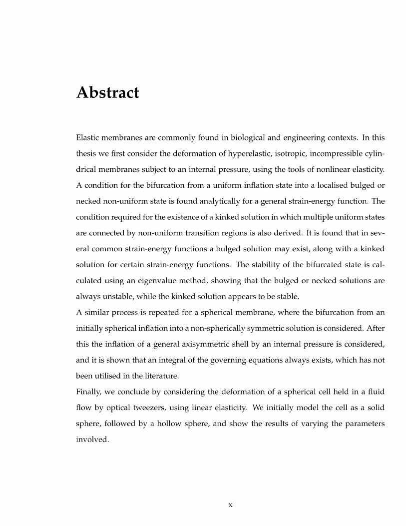
Elastic membranes are commonly found in biological and engineering contexts. In this

thesis we first consider the deformation of hyperelastic, isotropic, incompressible cylin-

drical membranes subject to an internal pressure, using the tools of nonlinear elasticity.

A condition for the bifurcation from a uniform inflation state into a localised bulged or

necked non-uniform state is found analytically for a general strain-energy function. The

condition required for the existence of a kinked solution in which multiple uniform states

are connected by non-uniform transition regions is also derived. It is found that in sev-

eral common strain-energy functions a bulged solution may exist, along with a kinked

solution for certain strain-energy functions. The stability of the bifurcated state is cal-

culated using an eigenvalue method, showing that the bulged or necked solutions are

always unstable, while the kinked solution appears to be stable.

A similar process is repeated for a spherical membrane, where the bifurcation from an

initially spherical inflation into a non-spherically symmetric solution is considered. After

this the inflation of a general axisymmetric shell by an internal pressure is considered,

and it is shown that an integral of the governing equations always exists, which has not

been utilised in the literature.

Finally, we conclude by considering the deformation of a spherical cell held in a fluid

flow by optical tweezers, using linear elasticity. We initially model the cell as a solid

sphere, followed by a hollow sphere, and show the results of varying the parameters

involved.

x

Chapter 1

Introduction

1.1 Introduction

Membranes are found in many biological contexts, where the word is used to define a

thin layer of tissue which delimits the boundary between two spaces (Humphrey 2003).

For example, animal and plant cells (eukaryotes) are surrounded by the cell surface mem-

brane, the plasmalemma, which separates the contents of cells from their environment

and acts as a partially permeable barrier controlling exchange with the external environ-

ment (Soper et al. 1990). At a larger scale, blood vessels and the lens of the eye may be

considered as biological membranes (Humphrey 1998).

In mechanics, such a solid structure is denoted a shell, rather than a membrane (Libai

and Simmonds 1998). An additional restriction is given on the definition of a membrane,

which is that a membrane is a thin shell considered to have negligible resistance to bend-

ing, where bending moments and transverse shears are considered insignificant com-

pared to in-plane loadings (Libai and Simmonds 1998). Humphrey (1998) showed that

many biological membranes may be modelled as mechanical membranes in this way, and

gives a very informative review of the techniques with which to treat elastic biological

membranes. Throughout this text the mechanical definition of membrane will be used.

1

Here we shall model membranes as elastic, that is as solids which deform instanta-

neously in response to an applied load, and return to their original shape after the load

is removed. This is an approximation to the reality for biological applications, where

time-dependent (viscoelastic) or permanent (plastic) deformations often occur. As in all

mathematical modelling we hope that investigating this initial case will be instructive,

despite its limitations.

Biological cells exist in a complex environment, where they respond to mechanical, bi-

ological and environmental signals to change their form and function (Bao and Suresh

2003). We are therefore interested in the stresses and strains which the cells experience,

as this is known to be biologically relevant for various different cells, such as endothelial

cells (Frangos et al. 1988, McCormick et al. 2001), and more generally by Chicurel et al.

(1998).

Barthes-Biesel (1980) define a microcapsule to be a thin elastic membrane surrounding

a Newtonian incompressible fluid, which can potentially support large deformations.

They both occur naturally, such as cells and eggs, and are synthesised for various in-

dustrial applications such as the food, cosmetic and biomedical industries (Chang and

Olbricht 1993). The main difficulty involved in modelling the behaviour of the microcap-

sule is the coupling between the fluid problem and the elasticity problem. The deforma-

tion of such initially spherical capsules in shear flows has been studied by Barthes-Biesel

and Rallison (1981), Ramanujan and Pozrikidis (1998), Walter et al. (2001) and Finken

and Seifert (2006) amongst others. Modelling red blood cells, with their complex geom-

etry but biological significance, as such a microcapsule has been undertaken, as in the

studies by Skotheim and Secomb (2007) and Abkarian et al. (2007). Assuming that a con-

stant pressure is exerted on the inside face of the membrane, it is possible to simplify the

problem by not explicitly modelling the fluid.

It is worth noting that this concept of the mechanical response of a cell coming entirely

from the cell membrane is an extremely simplistic model of the underlying biological

structure (Ingber 2003). In particular, the internal cytoskeleton, composed of intercon-

2

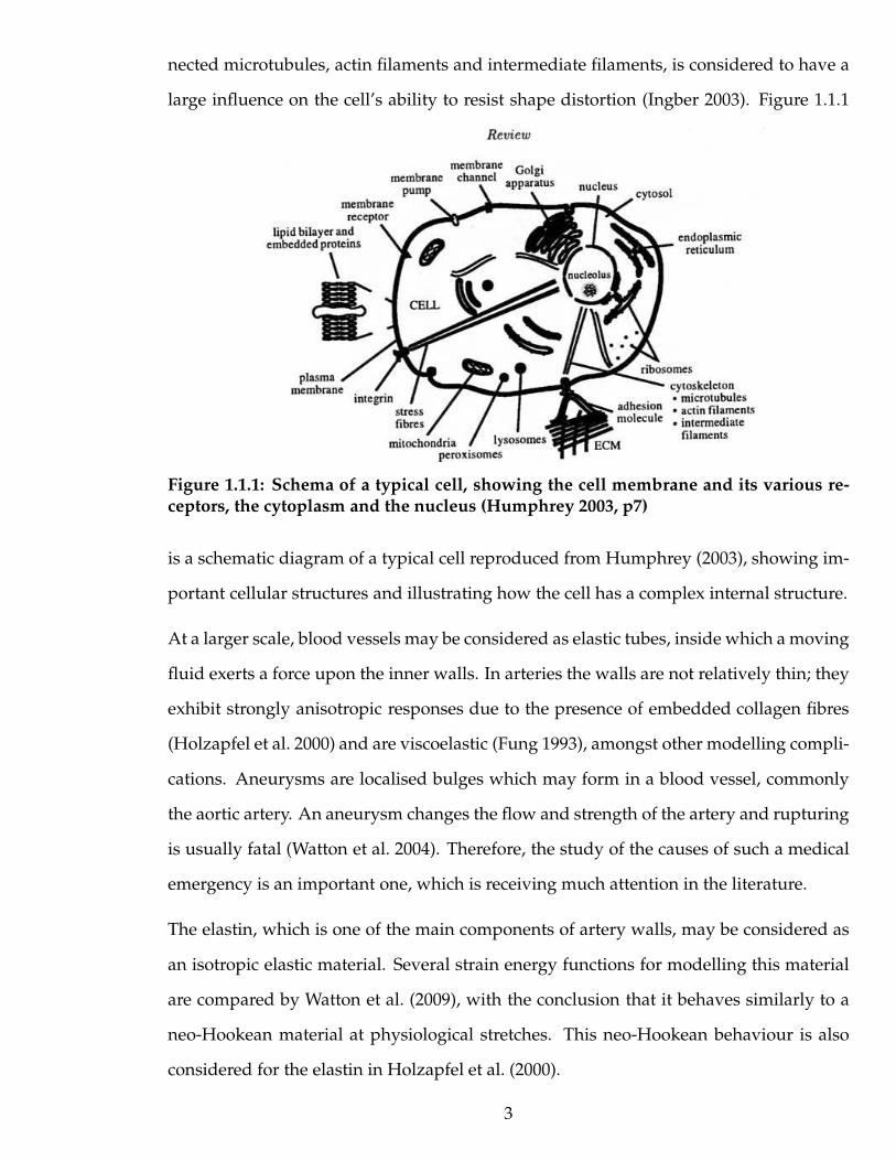
nected microtubules, actin filaments and intermediate filaments, is considered to have a

large influence on the cell’s ability to resist shape distortion (Ingber 2003). Figure 1.1.1

Figure 1.1.1: Schema of a typical cell, showing the cell membrane and its various re-ceptors, the cytoplasm and the nucleus (Humphrey 2003, p7)

is a schematic diagram of a typical cell reproduced from Humphrey (2003), showing im-

portant cellular structures and illustrating how the cell has a complex internal structure.

At a larger scale, blood vessels may be considered as elastic tubes, inside which a moving

fluid exerts a force upon the inner walls. In arteries the walls are not relatively thin; they

exhibit strongly anisotropic responses due to the presence of embedded collagen fibres

(Holzapfel et al. 2000) and are viscoelastic (Fung 1993), amongst other modelling compli-

cations. Aneurysms are localised bulges which may form in a blood vessel, commonly

the aortic artery. An aneurysm changes the flow and strength of the artery and rupturing

is usually fatal (Watton et al. 2004). Therefore, the study of the causes of such a medical

emergency is an important one, which is receiving much attention in the literature.

The elastin, which is one of the main components of artery walls, may be considered as

an isotropic elastic material. Several strain energy functions for modelling this material

are compared by Watton et al. (2009), with the conclusion that it behaves similarly to a

neo-Hookean material at physiological stretches. This neo-Hookean behaviour is also

considered for the elastin in Holzapfel et al. (2000).

3

In this thesis, we start by considering the inflation of a cylindrical, isotropic, incompress-

ible, elastic membrane subject to an internal pressure, looking in particular for solutions

which are localised in their non-uniformity along the length of the tube. We find an ex-

pression for the critical value of the pressure at which such a non-uniform solution may

exist, which is given in terms of a general strain-energy function and is therefore appli-

cable to a wide range of materials. Depending on the form of the strain-energy function,

there may also exist what we call a ‘kinked’ solution, where uniform sections of different

radii are connected by non-uniform transition regions. This solution is connected to the

existence of a Maxwell line in the pressure-volume diagrams, in the same way as in other

solid mechanics problems such as phase transitions in bars (Ericksen 1975) and propa-

gating necks in metals (Hutchinson and Neale 1983). We also find an analytic expression

for the shape of the bulge or neck close to the bifurcation point, as well as showing its

existence further from the bifurcation point.

Although bifurcated states may exist, they are not necessarily observable if they are un-

stable with respect to small perturbations. We therefore follow the derivation of the bi-

furcation condition with a stability analysis of the bulged or necked solution close to

the bifurcation point, in which we conclude that this weakly nonlinear solution is unsta-

ble. We then investigate the stability of the general bulged or necked state, using both

the techniques of spectral analysis and energy minimisation. We conclude that the bi-

furcated state is definitely unstable and we suggest that the kinked solution is probably

stable.

After our investigation of the inflation of a cylindrical membrane, we turn our attention

to the case of an initially spherical membrane instead. Here, instead of localised solutions

we find non-axisymmetric modal perturbations on the basic shape. We re-derive the bi-

furcation condition given by Haughton and Ogden (1978b) and Chen and Healey (1991),

using a different method which exploits the existence of an integral of the governing

equations.

We then consider the inflation of a general axisymmetric shell by including contributions

4

to the energy of the deformation from bending as well as from stretching, using the two-

dimensional membrane theory. We show that the integral of the governing equations

used in both the previous studies must exist for a shell of any undeformed shape, not

just a cylindrical or spherical membrane.

Finally, we look at the deformation of a spherical cell which is held immobile in a fluid

flow in optical tweezers, where the cell is restrained by the force produced by a focused

laser (Henon et al. 1999). We model this as part of a EPSRC/BBSRC grant on stem cells.

Baesu et al. (2004) discuss how important the non-destructive testing of such cells is,

and how optical tweezers are a useful method in such testing. Lim et al. (2006) com-

pare various mechanical models, and discuss how the experimental technique which is

being studied should influence the model which is used. In particular, if a low-force,

small-deformation technique such as optical tweezers is used then modelling the cell as

a linear elastic solid is viable. We therefore first take the cell to be a solid elastic body

and then a thin elastic shell, using only linear elasticity. As linear elasticity is only valid

for small deformations, we are interested in the value of the parameters at which the dis-

placements become large and the linear approximation is no longer valid, along with the

stresses induced on the cell up to this point.

Much of the content of Chapters 3, 4 and 5 has been published in two journal articles,

Fu et al. (2008) and Pearce and Fu (2010), although the material is presented here in a

self-contained manner.

5

Chapter 2

Mathematical Preliminaries

2.1 Continuum Mechanics

2.1.1 Introduction

In this section we outline the theory of continuum mechanics, before specialising to de-

formations of solid materials, specifically those which may be described as elastic, which

will then be used throughout the remainder of the thesis. In particular, the majority of

the chapters will focus on the theory of large deformations, where the linear approxima-

tion is not valid. The formulation here is standard in the literature, for more details see,

Ogden (1997), Holzapfel (2000) and Bertram (2008) as well as the individual citations in

the text.

2.1.2 Bodies and Configurations

A body B is a set of material points, or particles, each of which can be mapped to a point

in Euclidean space and is uniquely represented by a position vector at each time t. The

distribution of the points comprising the body in Euclidean space at a specific time is

called a configuration of the body.

6

We define Br, the reference configuration, to be a stress-free configuration of the body prior

to any deformation. Associated with each point in Br is a position vector X, relative to

an origin O in a coordinate system with basis vectors (Ei), where we use bold letters to

denote a vector or tensor. We shall also use undeformed to refer to the reference configu-

ration.

Additionally, we define Bt as the current configuration at time t > 0, and let x be the

position vector of a point in the body relative to O in a coordinate system with basis

vectors (ei). Again, we also denote this the deformed configuration. As Br and Bt are

different configurations of the body B, there must exist a bijective mapping fromBr toBt,

which we denote by χ. Therefore, we have x = χ (X, t), where the explicit dependence

on t is shown. Capital letters will be used wherever possible to denote quantities in

the reference configuration, while lower case versions of the same letters are used to

represent the corresponding quantities in the current configuration.

We shall require the two coordinate bases, (Ei) and (ei), to be orthogonal but not nec-

essarily Cartesian. It is possible to use non-orthogonal coordinate bases in continuum

mechanics, for example see Eringen (1962), although it is not required in this thesis and

therefore will not be discussed here. In general these two coordinate systems may be

different, though it is often convenient in applications for them to be identical, and this

will be the case here.

2.1.3 Tensor Algebra

This section introduces several results in tensor algebra which are required for this thesis,

but is in no way complete. The following books give an excellent introduction to the

use and theory of tensors, Ogden (1997), Spencer (1980), Chadwick (1999) and Bertram

(2008).

First we introduce the concept of the tensor product, denoted by ⊗, in that for any two

vectors u and v there exists a tensor product defined by its action on an arbitrary vector

7

a,

(u ⊗ v) · a = (a · v)u (2.1.1)

In component form, if the two vectors have expressions relative to the basis (ei), u =

uiei,v = viei, the tensor product may be written as

u⊗ v = uivjei ⊗ ej , (2.1.2)

where in (2.1.2), and elsewhere throughout this work unless stated otherwise, the sum-

mation convention is assumed. That is, whenever a Latin sub- or superscript is repeated

in an expression it is taken to imply a sum over that index between 1 and 3. The identity

tensor, I, may be written as,

I = ei ⊗ ei. (2.1.3)

For all coordinate systems we have the following expression for the total differential,

using the chain rule,

dx =∂x

∂sidsi ≡ gidsi, (2.1.4)

where si are any set of coordinates and gi are metric tensors associated with this co-

ordinate system. We now specify the values of these functions with respect to several

common coordinate systems. In Cartesian coordinates we find,

s1 = x1, s2 = x2, s3 = x3, g1 = ex, g2 = ey, g3 = ez, (2.1.5)

whereas for cylindrical polar coordinates,

s1 = r, s2 = θ, s3 = z, g1 = er, g2 = reθ, g3 = ez, (2.1.6)

and for spherical polar coordinates,

s1 = r, s2 = θ, s3 = φ, g1 = er, g2 = reθ, g3 = r sin θeφ. (2.1.7)

8

We then also define a dual metric basis, which is a set of vectors gi such that the following

orthogonality relation holds,

gi · gj = δij, (2.1.8)

which as we have assumed that the gi are an orthogonal set gives,

gi = gi/(|gi|2

). (2.1.9)

The gradient of a vector, which gives a tensor, may then be defined as,

grad u =∂u

∂si

⊗ gi. (2.1.10)

We also introduce the divergence of a tensor, which results in a vector, and is given by

div T = gi · ∂T∂si

. (2.1.11)

In particular, we will use cylindrical coordinates throughout this thesis, and therefore we

give an explicit result for (2.1.10) by writing u = urer + uθeθ + uzez, and using (2.1.6),

grad u =∂u

∂r⊗ er +

∂u

∂θ⊗ eθ

r+∂u

∂z⊗ ez

= ur,rer ⊗ er + uθ,reθ ⊗ er + uz,rez ⊗ er (2.1.12)

+(ur,θ

r− uθ

r

)

er ⊗ eθ +(uθ,θ

r+ur

r

)

eθ ⊗ eθ +uz,θ

rez ⊗ eθ

+ ur,zer ⊗ ez + uθ,zeθ ⊗ ez + uz,zez ⊗ ez

where a comma denotes differentiation with respect to that variable. In (2.1.12) the for-

mulae for the differentiation of the unit vectors in cylindrical coordinates, ∂er

∂θ= eθ,

∂eθ

∂θ=

−er, have been used. Similarly, if a second order tensor T is given by T = Tijei ⊗ ej

where (1, 2, 3) = (r, θ, z), the specialisation of (2.1.11) for cylindrical coordinates is given

9

by,

div T =

(

Trr,r +Trθ,θ

r+ Tzr,z +

Trr − Tθθ

r

)

er (2.1.13)

+

(

Trθ,r +Tθθ,θ

r+ Tzθ,z +

Tθr + Trθ

r

)

eθ (2.1.14)

+

(

Trz,r +Tθz,θ

r+ Tzz,z +

Trz

r

)

ez (2.1.15)

We also introduce the notations Grad and Div as being the gradient and divergence de-

fined in the same way but with respect to the undeformed configuration, with an appro-

priate change in the si from xi to Xi, and from ei in (2.1.4) to Ei.

2.1.4 Deformation Gradient

We are interested in the deformation from the given reference configuration to a current

configuration, without taking into account any intermediate steps. Indeed, we are chiefly

interested in problems with no explicit time dependence and are therefore interested in

quasi-static deformations where we look at states in which the equilibrium equations are

satisfied.

With this in mind, as we are interested in how the particles of the body move from a

point X in the reference undeformed configuration to a point x in the current deformed

configuration, we define the deformation gradient tensor F as the gradient of x with

respect to X,

F = Grad x =∂x

∂Xj

⊗Ej, (2.1.16)

where the repeated index represents the sum over j = 1, 2, 3 as mentioned previously.

Equation (2.1.16) allows us to determine how a neighbourhood of X is locally deformed,

and we can naturally write the following equation for the deformation of line elements

between the two configurations given by,

dx = FdX, (2.1.17)

10

where dX and dx are infinitesimal line elements in the reference and current configu-

rations respectively. The deformation gradient therefore enables us to transform line

elements between the two configurations. An important conclusion from (2.1.17) is that

F must be non-singular, else there exists some non-zero line elements X which vanish

under the deformation, which is physically unacceptable.

Taking three vectors in the reference configuration, X(1),X(2),X(3), we define an infinites-

imal volume element in the reference configuration as,

dV = [dX(1), dX(2), dX(3)], (2.1.18)

and we may use basic tensor theory (Spencer 1980) to deduce that

dv = JdV, (2.1.19)

where J = detF > 0 is the local volume change between the two configurations and dv

is the corresponding parallelepiped in the deformed configuration. Clearly, J is required

to be strictly positive to ensure that volumes remain positive, and therefore physical,

after deformation. A material is said to be incompressible if the volume does not change

under any deformation, leading to the condition J ≡ 1 for all X.

As F is a non-singular tensor with a positive determinant, the polar decomposition the-

orem (Chadwick 1999, Antman 2005) enables us to write it uniquely as,

F = RU = VR, (2.1.20)

where R is a proper orthogonal tensor and U,V are positive definite symmetric tensors.

This decomposition (2.1.20) represents a stretch U, followed by a rotation R, or a rotation

R followed by a stretch V. It may be shown that the two rotations here are identical, see

for example Ogden (1997).

As U is a positive definite symmetric tensor, it may be written in a diagonal form with

11

respect to a particular basis as,

U =

3∑

i=1

λiui ⊗ ui, (2.1.21)

where the axes (ui) are denoted as the principal axes of stretch, and the λi are known as

the principal stretches. In this decomposition, λi are the eigenvalues of U and (ui) are

the corresponding eigenvectors. A similar decomposition may be used on V, resulting

in the same principal stretches but rotated axes, given by vi = Rui.

We define the right Cauchy-Green deformation tensor, C, as

C = FT F = U2 =

3∑

i=1

λ2i u

i ⊗ ui, (2.1.22)

where a superscript T denotes the transpose of a tensor and (2.1.21) has been used to

express C as diagonal with respect to the basis (ui). C is clearly symmetric as(FTF

)T=

FT(FT)T

= FTF. C is also positive definite as, for a non-zero arbitrary vector a ∈ R3,

a · Ca = a · FTFa = Fa · Fa = |Fa|2 > 0.

We also define the Green strain tensor, E, as

E =1

2

(FTF − I

), (2.1.23)

where I is the identity tensor.

The displacement of a particle is defined as u = x−X, and therefore x = X + u. We also

note the following relation defining the displacement gradient Grad u,

F = Grad x = I + Grad u. (2.1.24)

The velocity of a point x is given by

v ≡ x =∂

∂tx (X, t) , (2.1.25)

where a superimposed dot represents differentiation with respect to t, and this expresses

12

the partial derivative with respect to t at a fixed X. We also define a velocity gradient

tensor L as,

L = grad v. (2.1.26)

We immediately note the connection, Grad v = (grad v)F = LF, where the first equation

comes from (2.1.16). Similarly, we can write Grad v = ∂∂t

Grad x = F, provided that the

partial derivatives are suitably continuous which we will assume here. Therefore we find

the following relation,

F = LF. (2.1.27)

We also note the relation

tr L = tr (grad v) = div v, (2.1.28)

which follows from the definition (2.1.26).

2.1.5 Conservation of mass

It is assumed that there exists a scalar field, ρ, which is the mass density of the material of

the body defined in the current configuration Bt. Let Rt be an arbitrary region in the cur-

rent configuration, then as the body deforms the mass of the material in this region must

not change. Therefore we require the following equation representing the conservation

of mass to hold,

d

dt

∫

Rt

ρ dv = 0. (2.1.29)

By converting the integral over Rt into an integral over the equivalent region in the refer-

ence configuration, Rr, we may take the derivative with respect to time inside the integral

as Rr does not depend on t. Therefore (2.1.29) becomes,

d

dt

∫

Rt

ρ dv =

∫

Rr

d (ρJ)

dtdV =

∫

Rt

(

ρ+ ρJ

J

)

dv = 0. (2.1.30)

As the region Rt is arbitrary, the equation Jρ + ρJ = 0 must hold throughout the con-

figuration, where it has been assumed that this function is continuous. We can therefore

13

integrate and write ρJ = ρr, where ρr is the density of the material in the undeformed

configuration.

Using the tensor identity, ∂∂t

(detF) = detF tr(

F−1F)

(Chadwick 1999) as well as (2.1.26)

and (2.1.27), we find

J = J tr L = J div v. (2.1.31)

Using (2.1.31), we therefore find the conservation of mass (2.1.30) becomes,

ρ+ ρdiv v = 0 (2.1.32)

which must hold throughout the body. If the density is constant, which is true for an

incompressible material as J = 0, then (2.1.32) reduces to div v = 0.

2.1.6 Conservation of Momentum

We consider a small region of the current configuration, on whose faces the forces from

the remainder of the body act. These forces are known as tractions, which are represented

by vectors which depend on the position in the configuration, along with the normal to

the excised surface n, given by t (x,n). This description of the tractions is known as

Cauchy’s stress principle, and is regarded as an axiom (Ogden 1997).

Therefore the forces which act on the surface of the arbitrary region in the current con-

figuration ∂Rt are given by∫

∂Rtt (x,n) da. If there are forces acting throughout the body,

such as gravity, then these body forces give a contribution to the force in the current

configuration which is given by∫

Rtρbdv, where b is the body force per unit mass.

The linear momentum of the material in the region Rt is given by mass multiplied by

velocity, i.e.∫

Rtρvdv. Therefore, using Newton’s second law, in the form Force =

ddt

(Momentum), along with the previous considerations, the following equation must

hold,∫

∂Rt

t (x,n) da+

∫

Rt

ρb dv =d

dt

∫

Rt

ρv dv. (2.1.33)

14

The right hand side of (2.1.33) may be written, by converting from Rt to Rr, taking the

derivative inside and converting back to Rt, as

d

dt

∫

Rt

ρv dv =

∫

Rt

d

dt(ρvJdV ) =

∫

Rt

˙(ρvJ)

Jdv =

∫

Rt

(

ρv + ρv + ρJ

Jv

)

dv =

∫

Rt

ρa dv,

(2.1.34)

where the conservation of mass has been used in the last equality and a = v. Therefore

(2.1.33) may be written,

∫

∂Rt

t (x,n) da =

∫

Rt

ρ (a − b) dv. (2.1.35)

2.1.7 Equations of Motion

We now state without proof Cauchy’s Theorem, as given in Ogden (1997) or Holzapfel

(2000), which states that provided that the traction vector t (x,n) is continuous in x then

it depends linearly on n, and therefore there exists a second-order tensor σ independent

of n such that,

t (x,n) = σT (x, t) · n (2.1.36)

where σ is expected to be a function of x and t. The tensor σ is called the Cauchy stress

tensor. The components of σ, σij , are the stresses acting in the direction j on the i plane,

and therefore the components σii are normal stresses while the components σij , i 6= j, are

shear stresses.

The equation of linear momentum, (2.1.35), therefore becomes,

∫

∂Rt

σT · n da =

∫

Rt

ρ (a − b) dv. (2.1.37)

Using the divergence theorem, a standard result in vector calculus, the left hand side of

(2.1.37) may be written as,

∫

∂Rt

σT · n da =

∫

Rt

divσ dv, (2.1.38)

15

and therefore, as Rt is an arbitrary region, we find the following equation of motion,

divσ = ρ (a− b) . (2.1.39)

A similar procedure as that which produced this equation of motion may be used to

derive an equation for the angular momentum, which reduces to

σ = σT , (2.1.40)

implying that σ must be a symmetric tensor. For details of this see Spencer (1980) or

Ogden (1997). Throughout this thesis no body forces will be considered, and therefore

we set b = 0. If the material is in equilibrium then a = 0, and (2.1.39) becomes the

equilibrium equations,

divσ = 0. (2.1.41)

We also wish to define the nominal stress tensor, S, which is a measure of the stress in

the reference configuration. This is related to σ by,

S = JF−1σ, (2.1.42)

and therefore we may write (2.1.41) as,

Div S = 0 (2.1.43)

2.1.8 Constitutive Models

Equations (2.1.32), (2.1.39) and (2.1.40) give 7 relations between 13 unknowns, (ρ,v,σ), or

4 relations between 10 unknowns after taking σ to be symmetric. The remaining six rela-

tions need to be determined from the constitutive equations representing the properties

of the material making up the body. So far these governing equations are valid for any

continuum of material, whether solid or fluid; elastic, viscoelastic or plastic. The speci-

16

fication of the remaining six relations must be chosen in an appropriate way depending

on the material of the body under consideration. These relations come from considering

how the stresses in the material are related to the strains, from experimental and physical

observations. The relation for a linear elastic material was first given by Hooke in 1678 as

‘As the extension, so the force’, stating that the stress is proportional to the strain, which

we may generalise to multiple dimensions and write as,

Stress ∝ Strain, (2.1.44)

where the proportionality constant implied by (2.1.44) is an elastic modulus. The precise

form of this relationship will be discussed later. A Newtonian fluid, named after Isaac

Newton, is a fluid whose relation between stress and strain is given by,

Stress ∝ d Strain

dt, (2.1.45)

where the stress in the fluid is proportional to the rate of strain rather than the strain

itself. The proportionality constant implied by (2.1.45) is a viscosity, and represent the

resistance of the fluid-fluid interactions. Many common liquids and gases are such New-

tonian fluids.

Some materials behave like solids in some circumstances and like fluids in other circum-

stances. These viscoelastic materials have relationships which involve both the amount

of, and rate of, stress and strain. These materials exhibit time-dependent behaviour, in-

cluding creep and relaxation. For example, the Kelvin-Voigt viscoelastic model relates

the stress to both the amount and rate of strain,

Stress ∝(

Strain,d Strain

dt

)

. (2.1.46)

There are also other models for viscoelastic materials which include the rate of stress into

the constitutive equations. In addition, materials may behave plastically, where the stress

depends both on the history of the deformation as well as the current state.

17

2.1.9 Elasticity

We wish to specify the equations of continuum mechanics which have been derived so

far to the case of elasticity. As discussed above, we therefore require the stress to be

proportional to the strain, and we also require that the Cauchy stress depends only on

the deformation gradient, without depending on the history or the path taken to reach

the point F, by assuming,

σ = g (F,X) , (2.1.47)

for some symmetric tensor valued function g, with g (I,X) = 0 so that the reference con-

figuration is stress-free. This assumption is known as Cauchy elasticity, the alternative of

allowing g to depend on higher-order gradients of F is possible but not considered here.

We will consider homogeneous materials from hereon, and therefore assume that σ does

not depend on X and will drop this argument from the definition of g.

In theory any tensor function g would be a potential choice for defining a constitutive

equation. However, choosing such a function at ‘random’, while mathematically possi-

ble, would not be physically meaningful due to violation of certain physical considera-

tions. In particular, it is necessary that the function g is objective. That is, the stresses

in the body must be independent of rigid-body motion after deformation has occurred

(Ogden 1997). The form of such a rigid-body motion is given by

x∗ = Q (t)x + c (t) , (2.1.48)

where Q is a proper orthogonal rotation tensor and c is a constant translation vector.

The corresponding deformation gradient, F∗, is given by an application of the chain rule

as F∗ = QF. Similarly, the stress tensor with respect to x∗ is given by σ∗ = QσQT .

Therefore a tensor-valued function g is an objective function of F if and only if,

g(F∗) = g(QF) = Qg(F)QT = σ∗, (2.1.49)

for each F and all rotations Q (Ogden 1997).

18

2.1.10 Isotropy

A body is isotropic relative to Br if the response of any small section of material cut from

Br is independent of its orientation in Br. For example, rubber is isotropic, but rubber

reinforced with metal strips in a specific direction is anisotropic. For isotropic materials

we have the additional requirement that the response function must be invariant under

rigid-body rotation prior to deformation, that is

g(FQ) = g(F), (2.1.50)

for each F and all rotations Q. On taking Q = RT in (2.1.50), we have

σ = g(F) = g(V), (2.1.51)

and therefore σ only depends on F through V. Therefore, combining (2.1.49) and (2.1.51),

we find that the response function must satisfy, for any rotation Q,

g(QTVQ) = QTg(V)Q. (2.1.52)

A tensor-valued function g which satisfies (2.1.52) is an isotropic tensor function of F.

The representation theorem, see for example Ogden (1997), states that any such second-

order isotropic tensor function must have the following representation,

g(V) = φ0I + φ1V + φ2V2, (2.1.53)

where the φi are functions of the three principal invariants of a three-dimensional second-

order tensor, given by tr V, 12((tr V)2 − tr (V2)) and detV (Spencer 1980). If a tensor is

given in spectral form as in (2.1.21) and (2.1.22), then these invariants may be written as,

19

for V,

i1 ≡ tr (V) = λ1 + λ2 + λ3

i2 ≡1

2[i21 − tr

(V2)] = λ1λ2 + λ1λ3 + λ2λ3 (2.1.54)

i3 ≡ detV = λ1λ2λ3,

or for the tensor C,

I1 ≡ tr (C) = λ21 + λ2

2 + λ23

I2 ≡1

2[I2

1 − tr(C2)] = λ2

1λ22 + λ2

1λ23 + λ2

2λ23 (2.1.55)

I3 ≡ detC = λ21λ

22λ

23.

where we have introduced the notations Ik and ik, which are used throughout this work

to represent the invariants of C and V respectively. These two sets of invariants may be

connected using I1 = i21 − 2i2, I2 = i22 − 2i1i3, I3 = i23.

2.1.11 Conservation of Energy

We now derive the law of conservation of energy, following the method presented in

Ogden (1997). We take the dot product of the equation of motion, (2.1.39), with the

velocity v, giving

(divσ) · v + ρ (b · v) = v · v, (2.1.56)

where v is the acceleration as defined earlier. We then rewrite the first term as,

div (σv) − tr (σL) + ρ (b · v) = v · v, (2.1.57)

where L is the velocity gradient defined in (2.1.26). Integrating (2.1.57) over the current

configuration, Bt, and using the divergence theorem and the conservation of mass we

20

result in,

∫

Bt

ρb.v dv +

∫

∂Bt

t · v da =d

dt

∫

Bt

1

2ρv · v dv +

∫

Bt

tr (σL) dv. (2.1.58)

In (2.1.58) the left hand side represents the rate of working of the forces applied to the

body, and the first term on the right hand side is the kinetic energy. If the deformation

is conservative and no energy is lost, then this remaining term must represent the stored

elastic energy. Rewriting this term as,

∫

Bt

tr (σL) dv =

∫

Br

Jtr (σL) dV, (2.1.59)

we may then interpret Jtr (σL) as the rate of increase of elastic energy per unit volume

in Br (Ogden 1997), which is the work done by the forces acting on the body.

2.2 Strain-Energy Functions

For an isotropic, homogenous material we now introduce a strain-energy function W (F)

which represents the stored elastic energy per unit undeformed volume of the material,

∂

∂tW (F) = Jtr (σL) . (2.2.1)

An elastic material satisfying (2.2.1) is said to be hyperelastic. We may then write,

∂

∂tW (F) =

∂W

∂Fij

∂Fij

∂t≡ tr

(∂W

∂FF

)

= tr

(∂W

∂FLF

)

= tr

(

F∂W

∂FL

)

, (2.2.2)

where we have used (2.1.27), and we define ∂W∂F

as the tensor whose components are

given by the convention,(∂W

∂F

)

ji

=∂W

∂Fij. (2.2.3)

21

Comparing (2.2.1) and (2.2.2) we find a relation between the strain-energy function and

the Cauchy stress,

Jσ = F∂W

∂F(2.2.4)

It is convenient to regard W as being either a function of the three stretches, W (λ1, λ2, λ3),

or the three invariants defined in (2.1.55). It is the character ofW which expresses the dif-

ferences between various materials, and prescribes the remaining constitutive equations

to complete the formulation of elastic deformations. Due to the isotropy of the material,

the strain-energy function must be a symmetric function of the three principal stretches

and hence

W (λ1, λ2, λ3) = W (λ1, λ3, λ2) = W (λ2, λ3, λ1) . (2.2.5)

A further restriction on W is that there is no stored energy or stress in the reference

configuration, Br, implying

W (1, 1, 1) = 0,∂W (1, 1, 1)

∂λi= 0, i ∈ 1, 2, 3. (2.2.6)

With respect to the principal stretches for an isotropic material, (2.2.4) becomes,

σi = J−1λi∂W

∂λi

, (2.2.7)

which are in the principal directions ui.

If the material is incompressible then J = detF = λ1λ2λ3 = 1, and therefore the deriva-

tives of (2.1.16) and (2.2.7) are no longer independent. We therefore introduce a pseudo-

strain-energy function, W = W (F) − p(detF − 1), where p is a Lagrange multiplier. It is

clear that once we apply the constraint, W is identical to W , and (2.2.4) becomes,

σ = F∂

∂F(W − p(detF − 1)) = F

∂W

∂F− pI, (2.2.8)

where we have used ∂ detF

∂F= F−1, and have applied the constraint after differentiation.

In doing tr (σL), the work done by the forces on the body, is not affected by p, and so the

22

constraint does no work as required.

In terms of the principal stretches, (2.2.8) becomes,

σi = λi∂W

∂λi− p, (2.2.9)

instead of (2.2.7).

The strain-energy function incorporates an elastic modulus, in units of Force/Area, which

corresponds to the shear modulus in infinitesimal, or linear, deformations and will be

denoted here by µ. We now present a variety of strain-energy functions for isotropic in-

compressible elastic solids which will be considered in later chapters. As was mentioned

above, the space of such functions is extremely large, in that any function of the two

invariants I1, I2 which satisfies (2.2.5) and (2.2.6) may be considered as a viable strain-

energy function, although there are other physical considerations.

2.2.1 Varga Strain-Energy Function

A simple strain-energy function when expressed with respect to the stretches is the Varga

strain-energy function. This function was described by Varga (1966) to model rubber for

small but not infinitesimal stretches of the order of 1.3 say. As a function of the stretches

it is given by

W = 2µ(i1 − 3) = 2µ(λ1 + λ2 + λ3 − 3), (2.2.10)

where µ is the infinitesimal shear modulus. The Varga strain-energy function is useful

for theoretical work due to its simple linear mathematical structure, but does not model

many physical behaviours observed in elastic materials.

23

2.2.2 Neo-Hookean Strain-Energy Function

The neo-Hookean strain-energy function is a generalisation of Hooke’s Law to the case

of nonlinear elasticity, that is that the extension is linearly proportional to the stress,

W =1

2µ(I1 − 3) =

1

2µ(λ2

1 + λ22 + λ2

3 − 3). (2.2.11)

The neo-Hookean model also has a simple mathematical structure while having much

wider physical application, particularly to the modelling of rubber at small to moderate

stretches of up to approximately 1.5. In particular, Muller and Strehlow (2004) show that

(2.2.11) is inappropriate for biaxial stretching above this range. Along with the Varga

strain-energy function, the neo-Hookean model is one of the most commonly used strain-

energy functions for analytical work due to their simplicity.

2.2.3 Mooney-Rivlin Strain-Energy Function

The Mooney-Rivlin is a more generalised model than the neo-Hookean, incorporating a

term involving I2, and does not follow Hooke’s Law for large deformations unless α = 0,

W =µ

2((1 − α)(I1 − 3) + α(I2 − 3)) . (2.2.12)

In this model there is a second parameter, α, which expresses the measure of nonlinearity

of the material. This strain energy function is known to model rubber to a good precision

(Muller and Strehlow 2004). When α = 0 this simplifies to the neo-Hookean strain-energy

function given in (2.2.11).

2.2.4 Gent Strain-Energy Function

The simplified Gent strain-energy function was first introduced by Gent (1996) to model

rubbers which are strain-hardening. Its derivation is from considering the hydrocarbon

24

chains, which comprise the rubber at an atomistic level, as being initially tangled and

unextended, which then straighten and become taut as the continuum is stretched. The

model has a second parameter, Jm, which represents the maximum value of J1 = I1 − 3

beyond which the hydrocarbon chains may not extend any further, and the strain-energy

function is given by

W = −1

2µJm log

(

1 − J1

Jm

)

. (2.2.13)

This Gent strain-energy function, along with a more complex version involving a term in

I2, have become popular models for a range of rubber and bio-materials. Its use has been

discussed in several papers including Horgan and Saccomandi (2003, 2006) and Ogden

et al. (2006) in the context of other so called ’finite-chain’ models, where the molecules

which make up the materials are initially compact and tangled until a specific expansion

ratio. Gent (1996) suggests that Jm = 97.2 or 114 are typical values of the parameter Jm

for rubber, whereas for human arteries Horgan and Saccomandi (2003) give a range for

Jm of between 0.422 and 3.93. The maximum stretch in any direction is given from the

definition of I1 by approximately√Jm + 3.

2.2.5 General Separable Strain-Energy Function

Ogden (1997) present the general form of a separable strain-energy function expanded in

terms of the stretches as

W S =

N∑

n=1

µn

αn(λαn

1 + λαn

2 + λαn

3 − 3) , (2.2.14)

with µn, αn ∈ R and µnαn > 0,∑N

n=1 µnαn = 2µ, for some N ≥ 1. The Varga and neo-

Hookean models discussed already fall into this category of strain-energy functions with

N = 1, α1 = 1, 2 respectively. Equation (2.2.14) is commonly known as the Ogden model

after it was introduced in Ogden (1972), with a set of constants based on experimental

measurements of rubber, given by µ1 = 1.491, µ2 = 0.003, µ3 = −0.023, α1 = 1.3, α2 =

5.0, α3 = −2.0. This set of constants has been used in many studies, and will be denoted

25

the Ogden model throughout this thesis.

Kyriakides and Chang (1991) fit such a strain-energy function to some rubber tubes, find-

ing µ1 = 617, µ2 = 1.86, µ3 = −9.79, α1 = 1.3, α2 = 5.08, α3 = −2.00, which when non-

dimensionalised with respect to µ gives very similar values as the Ogden model.

2.2.6 Fung Strain-Energy Function

Fung (1993) introduced a strain-energy function designed for the modelling of biological

soft tissues, which commonly feature strain-stiffening behaviour, such as healthy arterial

tissue as,

W =µ(eΓ(I1−3) − 1

)

Γ, (2.2.15)

where Γ is a positive parameter representing the degree of strain stiffening. In the limit as

Γ approaches zero, (2.2.15) reproduces the neo-Hookean strain-energy function (2.2.11).

2.3 Membrane Elasticity

An elastic shell may be defined as a three-dimensional elastic body with a dimension

which is much thinner than the other two, and therefore ǫ = H/R ≪ 1, where H is a

typical thickness in the thin direction and R is a typical lengthscale in the remainder of

the body (Libai and Simmonds 1998). This enables us to consider the deformation of

only the mid-plane of the elastic body through this thinner direction. An axishell is such

a shell which has symmetry around an axis. A membrane may then be defined as a shell

which has negligible resistance to bending (Libai and Simmonds 1998, Humphrey 2003).

There are three different classes of membrane theories which may be used, as detailed

below.

26

2.3.1 Membrane-Like Shells

The first of these membrane theories may be called a ‘membrane-like shell’ (Libai and

Simmonds 1998), which takes the shell theory of three-dimensional elasticity and then

neglects the contribution to strain-energy from bending in the shell theory. Then, from

the asymptotic expansion in the small-thickness variable, the ‘membrane assumption’ of

no stress through the thickness of the membrane, i.e. σ3 = 0, is a consequence in the

asymptotic approximation (Humphrey 1998, Haughton and Ogden 1978a).

In this formulation the thickness is included in the derivation, as λ3 is still included in

the governing equations. These equations explicitly allow the membrane to get thinner

via stretching in the other directions. The membrane may be considered as either com-

pressible or incompressible, although the assumption of incompressibility is commonly

used.

This is a common method of treating membranes, and a comprehensive derivation may

be found in Haughton and Ogden (1978a), Libai and Simmonds (1998) and Steigmann

(2007). In particular, Haughton and Ogden (1978a) give explicit expressions for the errors

introduced by the approximation, showing that the stress through the membrane is also

of order H/R, as do Kydoniefs (1969) and Erbay and Demiray (1995) for particular prob-

lems in cylindrical coordinates. A variational treatment of this problem has also been

considered, for example see Le Dret and Raoult (1996) and Chen (1997).

2.3.2 Simple Membranes

The second class of membrane theories occurs from considering the mid-plane of the

membrane as a two-dimensional sheet of elastic material embedded into a three-dimensional

space, entirely neglecting thickness effects through the membrane (Li and Steigmann

1995). Nadler and Rubin (2009) call this a ‘simple membrane’, and a consequence of

this reduction is that the stretch through the membrane λ3, does not appear directly in

the formulation and is therefore assumed to remain constant. The deformation gradient

27

becomes two-dimensional, and there are only two strain invariants and two principal

stretches rather than the three given in the three-dimensional theory.

The consequence of this is that, for instance, the equivalent of the neo-Hookean strain-

energy function would be W = µ2

(I1 − 2) = µ2

(λ21 + λ2

2 − 2), which is clearly different

to W = µ2

(λ2

1 + λ22 + λ−2

1 λ−22 − 3

). It is possible to define two-dimensional strain-energy

functions which have no counterpart in the three-dimensional theory (Haughton 2001),

as well as to use three-dimensional strain-energy functions in the two-dimensional the-

ory. It has been shown that the simple membrane and membrane-like shell approaches

give the same governing equations to first order in ǫ (Naghdi 1972, Haughton 2001,

Steigmann 2007), and it is the specification of the constitutive behaviour which varies be-

tween the two theories. Further details of simple membranes may be found in Humphrey

(1998), Libai and Simmonds (1998), Steigmann (2007) and a particularly concise deriva-

tion in Steigmann (2009).

2.3.3 Generalised Membranes

There is a third approach, denoted a ‘generalised membrane’ by Nadler and Rubin (2009),

which takes the ‘membrane-like shell’ and removes the curvature of the reference geom-

etry by assuming the reference state is flat. This has the benefit of simplifying the govern-

ing equations, but is still applicable to three-dimensional strain-energy functions unlike

the ‘simple membrane’. However, if the reference geometry is highly curved then this

theory will not give the same results as either of the two previous membrane theories or

the fully three-dimensional theory.

2.3.4 Wrinkling

In addition, when considering deformations of membranes using any of the above the-

ories, it is important to ensure that the membrane remains in tension, i.e. the principal

stresses remain positive throughout the deformations (Humphrey 1998). If compressive

28

stresses occur then the membrane may wrinkle, which is not included in the formula-

tion considered here. In particular, Andra et al. (2000) show that equilibrium states with

distributions of infinitesimal wrinkles are possible when bending stiffness is neglected

due to loss of convexity of the strain-energy function. For more details about the connec-

tion between wrinkling and compressive stresses as well as introducing quasiconvexity

to extend the theory to include this case see Pipkin (1986), Li and Steigmann (1995) and

Finken and Seifert (2006).

Throughout this thesis the first approach, of taking the membrane approximation from

the fully three-dimensional theory, will be used with the exception of Chapter 7 in which

the simple membrane theory is used to make a comparison between the two theories.

2.4 Linear Elasticity

2.4.1 Introduction

We will now consider the case of linear elasticity, that is the specification of the theory to

(infinitesimally) small deformations. In this we consider the case where the displacement

u is small, and will we neglect terms which are of order O(u2) or higher. We therefore

neglect any terms involving uiuj for any i and j, as well as products of derivatives of u.

This approximation is the source of the name linear elasticity, and does not imply that

the geometry must be linear.

2.4.2 Linearisation

On taking this linearisation and using (2.1.24), F = I + Grad u, the Green strain tensor E

becomes,

E =1

2

(FTF − I

)=

1

2

(

Grad u + (Grad u)T)

+ O(u2), (2.4.1)

29

or in component form in Cartesian coordinates, where we use ε to denote the components

of the tensor E,

εij =1

2

(∂ui

∂xj

+∂uj

∂xi

)

, (2.4.2)

where we have neglected the higher order terms. It should be noted that in non-Cartesian

coordinates there are extra terms corresponding to the derivatives of the basis vectors. In

the following Cartesian coordinates are used when component forms of the tensors are

given, although the tensor relations still hold for other coordinate systems, as part of the

definitions of tensors.

The diagonal components of the strain tensor, εii = ∂ui

∂xi(no sum), are the normal strains in

the directions given by i, and the off-diagonal components are given by εij = 12γij, i 6= j,

where γij denote the changes in angle between the initially orthogonal coordinate axes

(Lur’e 1964).

2.4.3 Hooke’s Law

The generalisation of Hooke’s Law mentioned in Section 2.1.8, corroborated by experi-

mental results, is given by the injective relation

σij = fij (ε11, ε12, ..., ε32, ε33) (2.4.3)

between the stresses σij and the strains εij (Sokolnikoff 1956). This relation holds for

elastic materials provided the stresses do not exceed the elastic limit of the material, after

which the material will fail, either from the beginning of irreversible plastic deforma-

tions, breaking or rupture.

Expressing the functions fij as a power series in the strains, εij, we may write,

σij = Aij + cijklεkl + O(ε2

ij

), (2.4.4)

30

where Aij and cijkl are the components of constant valued tensors of order two and four

respectively. In tensor form, (2.4.4) may be written,

σ = A + c : E + O(E2), (2.4.5)

where the central dots represent tensor contraction and A, c are the appropriate constant

valued tensors.

We require that the stresses σij vanish when the strains vanish, on the assumption that

the initial state is stress-free, and therefore we require that Aij = 0 for all i, j. Neglecting

the second order terms in ε, as per our assumption of small strains, will result in the

following constitutive relation for linear elasticity,

σij = cijklεkl, (2.4.6)

where the 81 coefficients cijkl in general vary throughout the material. If the cijkl are in-

dependent of the position of the point then the material is homogeneous and we will

henceforth make this assumption (Barber 2004). As the tensor σ must be symmetric to

satisfy the equation of angular momentum, the coefficients cijkl are symmetric with re-

spect to the indices i and j, so cijkl = cjikl. We can also assume, without loss of generality,

that the coefficients are therefore symmetric with respect to the indices k and l. This may

be proved by reducing cijkl into a symmetric and an anti-symmetric part given by

cSijkl =1

2(cijkl + cijlk) , cAijkl =

1

2(cijkl − cijlk) , (2.4.7)

whence cSijkl is symmetric in k and l and cAijkl is antisymmetric in the same indices. Thus

the coefficients can be expressed as cijkl = cSijkl + cAijkl, so (2.4.6) can be written as:

σij = cSijklεkl + cAijklεkl. (2.4.8)

However, the second term in this expression vanishes as cAijkl = −cAijlk by definition and

31

εkl = εlk from the symmetry of E.

Thus we can regard the coefficients cijkl as being symmetric with respect to both i, j and

k, l, and hence there are 36 independent coefficients cijkl. For notational convenience we

introduce the following notation for the six independent components of the stresses and

strains, (Landau and Lifshitz 1986)

σ11 = σ1, σ22 = σ2, σ33 = σ3, σ23 = σ4, σ31 = σ5, σ12 = σ6 (2.4.9)

ε11 = ε1, ε22 = ε2, ε33 = ε3, 2ε23 = ε4, 2ε31 = ε5, 2ε12 = ε6, (2.4.10)

which introduces a factor of two into the off-diagonal elements of the strain tensor. This

enables us to write concisely the six equations resulting from (2.4.6) as

σi = cijεj , (2.4.11)

where the cij are the 36 independent elastic moduli. The number of independent con-

stants reduces to 21 in the case where there exists a strain-energy function W = 12cijεiεj

with the property ∂W∂εi

= σi. As the quadratic form of W is always symmetric it follows

that cij = cji and hence the reduction to merely 21 constants. The existence of the strain-

energy function W has been argued using the first and second laws of thermodynamics

(Sokolnikoff 1956). For a completely anisotropic material these 21 constants are the re-

quired minimum, though material symmetries reduce the number of constants which

are independent. Sokolnikoff (1956) point out that in the derivation of (2.4.11) the com-

ponents of strain εij use the undeformed, or Lagrangian, coordinates while the stress

components σij are functions of the deformed, or Eulerian, coordinates. If the displace-

ments are small, which we have assumed here, then this distinction is not required, but

for large deformations this is not the case. Hence this formulation is only valid when the

displacement derivatives are small compared to one.

For the case where the material is isotropic the number of elastic constants reduces

to merely two. Landau and Lifshitz (1986) show that the stress-strain relationship for

32

isotropic elastic bodies may be written,

σik = λεllδik + 2Gεik, (2.4.12)

or, in tensor form,

σ = λtr (E) I + 2GE, (2.4.13)

where λ is the first Lame constant, G is the shear modulus of the material and tr (E) is

the trace of the tensor E. We use the alternative notation G here for the shear modulus in

order to reserve µ for when we use linear elasticity in Chapter 8. These two parameters

fully characterise the elastic properties of any isotropic material, although we will replace

the first Lame constant by the Poisson’s ratio, ν, given by ν = λ/ (2 (G+ λ)). The shear

modulus represents the resistance to shearing deformations and Poisson’s ratio governs

the relative contraction in the other two directions when the material undergoes unilat-

eral extension. For most materials Poisson’s ratio lies between 0 and 12, with the value

of 12

corresponding to an incompressible material. Negative values of the Poisson’s ratio

may also occur for specific materials with a high internal void fraction such as foams,

which are called auxetic.

2.4.4 Equilibrium equations

With (2.4.1) and (2.4.13) the displacements and stresses are coupled together. Along with

(2.1.41) and appropriate boundary conditions we have all the required equations to de-

termine the deformation of an elastic material under boundary conditions prescribing

either stresses or displacements. Eliminating the stress tensor σ in the equilibrium equa-

tions (2.1.41) by using (2.4.13) and (2.4.1), we find the equation for equilibrium in terms

of the displacements is given by:

1

1 − 2νgrad div u + ∇2u +

b

G= 0. (2.4.14)

33

Note that for an incompressible material, ν = 1/2, and hence λ → ∞, which reduces the

equilibrium equation (2.4.14) to

div u = 0. (2.4.15)

2.5 Compound Matrix Method

2.5.1 Introduction

In this section we present a method for solving eigenvalue problems in differential equa-

tions where the boundary conditions are prescribed at two ends, called the Compound

Matrix method. This method works well for differential equations which may contain

singularities or are otherwise numerically stiff. We also introduce the Evans function,

a complex analytic function whose zeros correspond to the eigenvalues (Evans 1975,

Alexander et al. 1990). The use of the Evans function ensures that the value of the eigen-

value found is not dependent on the point at which the solutions are matched. For fur-

ther details on the use and derivation of the compound matrix method see Ng and Reid

(1985) and Haughton (2009).

The method works on a set of n first-order linear ordinary differential equations, with

variable coefficients, which include a parameter ζ ∈ R, given by,

dy

dZ= A(Z; ζ) · y, a ≤ Z ≤ b (2.5.1)

where y(Z) = (y1(Z), y2(Z), . . . , yn(Z)) is the set of n dependent variables, Z is the inde-

pendent variable and A(Z) is a n×n matrix determined by the coefficients in the original

differential equations. In addition, one or both of the two endpoints a, b may be infinite.

We assume that there are associated boundary conditions, n in total, defined at one or

34

both ends of the range of Z by,

B(Z; ζ)y = 0 at Z = a (2.5.2a)

C(Z; ζ)y = 0 at Z = b, (2.5.2b)

where B and C are m1 × n and m2 × n matrices respectively, where m1 + m2 = n, and

are both known functions of Z and ζ . These boundary conditions (2.5.2) enable us to

specify any combination of boundary conditions at the endpoints. The case which we

will consider here is when n is even and m1 = m2 = m = n/2, although the method is

general and works for the case m1 6= m2. We wish to find the values of the parameter ζ

such that the system has a non-trivial solution which satisfies the boundary conditions,

and this value of ζ will be called an eigenvalue of the differential equations. Naively,

it is possible to guess a value of ζ , along with the unspecified components at Z = a,

and numerically integrate from a to b, varying both ζ and the unspecified components

at Z = a to satisfy the boundary conditions specified at b. However, this is naturally

inefficient and unsystematic. Instead, it would be common to use a determinant based

method in order to solve the equations, which we will describe here, before explaining

the compound matrix method.

2.5.2 Determinant Based Method

First, for a given value of ζ , assuming B has rank m we must be able to find m linearly

independent solutions to (2.5.2a) which we denote y(i)0 , i = 1, 2, . . . , m. Using these vec-

tors as our initial value at Z = a, we may integrate using (2.5.1) towards Z = b, leading

to a set of m independent solutions y(i)(Z), i = 1, 2, . . . , m. Therefore a general solution

which satisfies the left boundary condition and the equation (2.5.1) is given by,

y =m∑

i=1

kiy(i)(Z), (2.5.3)

for some constants ki.

35

We then proceed the same way from the right hand endpoint, denoting by y(i)0 , i = m +

1, m + 2, . . . , n the independent solutions to (2.5.2)2, and integrating towards Z = a,

resulting in a second set of m independent solutions y(i)(Z), i = m + 1, m + 2, . . . , n.

Therefore the general solution satisfying the right boundary condition is,

y =

n∑

i=m+1

kiy(i)(Z), (2.5.4)

for some further constants ki. We then impose that these two solutions must match at

some intermediate point Z = d. Therefore,

m∑

i=1

kiy(i)(Z) =

n∑

i=m+1

kiy(i)(Z), at Z = d, (2.5.5)

or equivalently,

N(d, ζ)c = 0, (2.5.6)

where c = (k1, k2, . . . , kn,−kn+1,−kn+2, . . . ,−kn)T and N(Z, ζ) is a matrix formed from

concatenating the n vectors, y(i)(Z)

N(Z, ζ) = [y(1),y(2), . . . ,y(m),y(m+1),y(m+2) . . . ,y(n)]. (2.5.7)

Therefore we need to iterate on ζ until the matching condition,

|N(d, ζ)| = 0, (2.5.8)

is satisfied. This matching condition is dependent on d as well as the value of ζ . It may

be shown that the following condition,

D(ζ) = e−∫

d

atrA(s,ζ)ds|N(d, ζ)| = 0, (2.5.9)

is independent of the value of d. This may be seen using the following matrix property

Chadwick (1999), d(detA)dx

= tr(adj (A) dA

dx

)for any square matrix A, that this function is

36

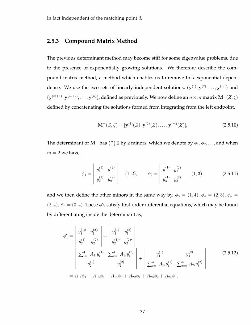
in fact independent of the matching point d.

2.5.3 Compound Matrix Method

The previous determinant method may become stiff for some eigenvalue problems, due

to the presence of exponentially growing solutions. We therefore describe the com-

pound matrix method, a method which enables us to remove this exponential depen-

dence. We use the two sets of linearly independent solutions, (y(1),y(2), . . . ,y(m)) and

(y(m+1),y(m+2), . . . ,y(n)), defined as previously. We now define an n×m matrix M−(Z, ζ)

defined by concatenating the solutions formed from integrating from the left endpoint,

M−(Z, ζ) = [y(1)(Z),y(2)(Z), . . . ,y(m)(Z)], (2.5.10)

The determinant of M− has(

nm

)2 by 2 minors, which we denote by φ1, φ2, . . ., and when

m = 2 we have,

φ1 =

∣∣∣∣∣∣∣

y(1)1 y

(2)1

y(1)2 y

(2)2

∣∣∣∣∣∣∣

≡ (1, 2), φ2 =

∣∣∣∣∣∣∣

y(1)1 y

(2)1

y(1)3 y

(2)3

∣∣∣∣∣∣∣

≡ (1, 3), (2.5.11)

and we then define the other minors in the same way by, φ3 = (1, 4), φ4 = (2, 3), φ5 =

(2, 4), φ6 = (3, 4). These φ’s satisfy first-order differential equations, which may be found

by differentiating inside the determinant as,

φ′1 =

∣∣∣∣∣∣∣

y(1)′1 y

(2)′1

y(1)2 y

(2)2

∣∣∣∣∣∣∣

+

∣∣∣∣∣∣∣

y(1)1 y

(2)1

y(1)′2 y

(2)′2

∣∣∣∣∣∣∣

=

∣∣∣∣∣∣∣

∑4i=1A1iy

(1)i

∑4i=1A1iy

(2)i

y(1)2 y

(2)2

∣∣∣∣∣∣∣

+

∣∣∣∣∣∣∣

y(1)1 y

(2)1

∑4i=1A2iy

(1)i

∑4i=1A2iy

(2)i

∣∣∣∣∣∣∣

= A11φ1 − A13φ4 − A14φ5 + A22φ1 + A23φ2 + A24φ3,

(2.5.12)

37

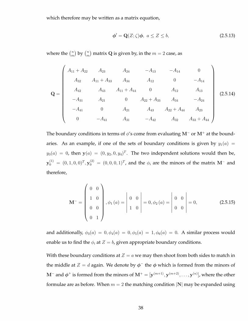
which therefore may be written as a matrix equation,

φ′ = Q(Z; ζ)φ, a ≤ Z ≤ b, (2.5.13)

where the(

nm

)by(

nm

)matrix Q is given by, in the m = 2 case, as

Q =

A11 + A22 A23 A24 −A13 −A14 0

A32 A11 + A33 A34 A12 0 −A14

A42 A43 A11 + A44 0 A12 A13

−A31 A21 0 A22 + A33 A34 −A24

−A41 0 A21 A43 A22 + A44 A23

0 −A41 A31 −A42 A32 A33 + A44

(2.5.14)

The boundary conditions in terms of φ’s come from evaluating M− or M+ at the bound-

aries. As an example, if one of the sets of boundary conditions is given by y1(a) =

y3(a) = 0, then y(a) = (0, y2, 0, y4)T . The two independent solutions would then be,

y(1)0 = (0, 1, 0, 0)T ,y

(2)0 = (0, 0, 0, 1)T , and the φi are the minors of the matrix M− and

therefore,

M− =

0 0

1 0

0 0

0 1

, φ1 (a) =

∣∣∣∣∣∣∣

0 0

1 0

∣∣∣∣∣∣∣

= 0, φ2 (a) =

∣∣∣∣∣∣∣

0 0

0 0

∣∣∣∣∣∣∣

= 0, (2.5.15)

and additionally, φ3(a) = 0, φ4(a) = 0, φ5(a) = 1, φ6(a) = 0. A similar process would

enable us to find the φi at Z = b, given appropriate boundary conditions.

With these boundary conditions at Z = a we may then shoot from both sides to match in

the middle at Z = d again. We denote by φ− the φ which is formed from the minors of

M− and φ+ is formed from the minors of M+ = [y(m+1),y(m+2), . . . ,y(n)], where the other

formulae are as before. When m = 2 the matching condition |N| may be expanded using

38

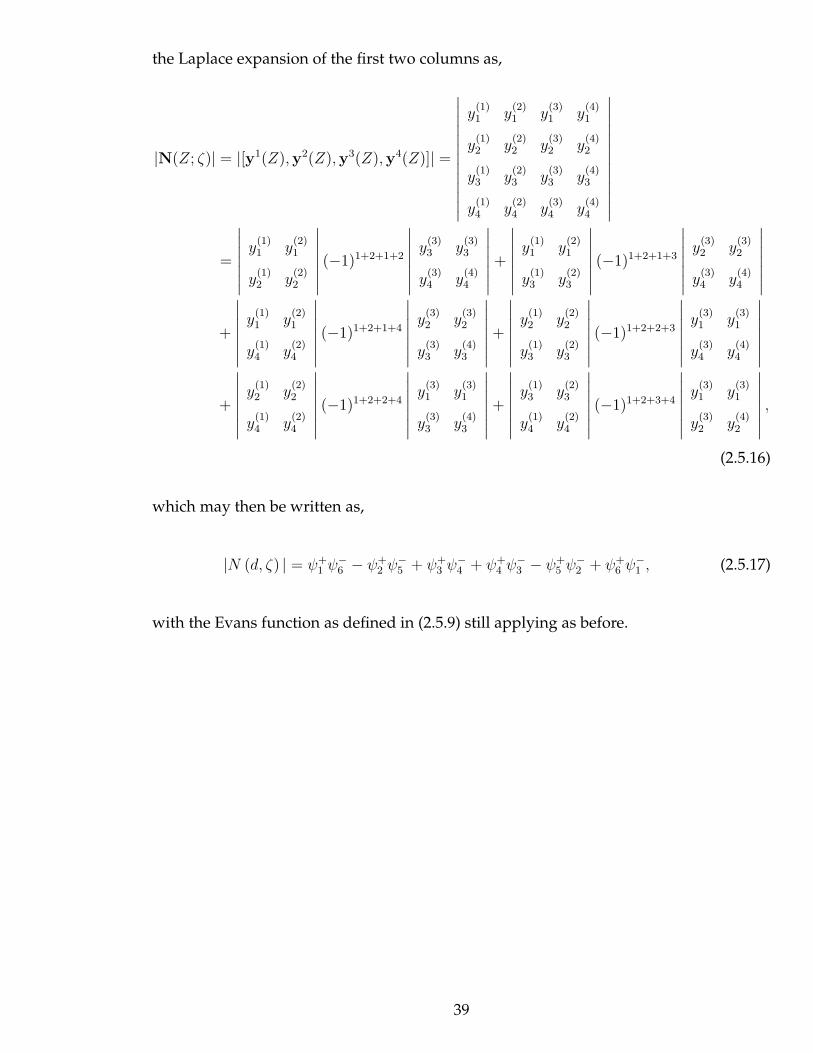
the Laplace expansion of the first two columns as,

|N(Z; ζ)| = |[y1(Z),y2(Z),y3(Z),y4(Z)]| =

∣∣∣∣∣∣∣∣∣∣∣∣∣

y(1)1 y

(2)1 y

(3)1 y

(4)1

y(1)2 y

(2)2 y

(3)2 y

(4)2

y(1)3 y

(2)3 y

(3)3 y

(4)3

y(1)4 y

(2)4 y

(3)4 y

(4)4

∣∣∣∣∣∣∣∣∣∣∣∣∣

=

∣∣∣∣∣∣∣

y(1)1 y

(2)1

y(1)2 y

(2)2

∣∣∣∣∣∣∣

(−1)1+2+1+2

∣∣∣∣∣∣∣

y(3)3 y

(3)3

y(3)4 y

(4)4

∣∣∣∣∣∣∣

+

∣∣∣∣∣∣∣

y(1)1 y

(2)1

y(1)3 y

(2)3

∣∣∣∣∣∣∣

(−1)1+2+1+3

∣∣∣∣∣∣∣

y(3)2 y

(3)2

y(3)4 y

(4)4

∣∣∣∣∣∣∣

+

∣∣∣∣∣∣∣

y(1)1 y

(2)1

y(1)4 y

(2)4

∣∣∣∣∣∣∣

(−1)1+2+1+4

∣∣∣∣∣∣∣

y(3)2 y

(3)2

y(3)3 y

(4)3

∣∣∣∣∣∣∣

+

∣∣∣∣∣∣∣

y(1)2 y

(2)2

y(1)3 y

(2)3

∣∣∣∣∣∣∣

(−1)1+2+2+3

∣∣∣∣∣∣∣

y(3)1 y

(3)1

y(3)4 y

(4)4

∣∣∣∣∣∣∣

+

∣∣∣∣∣∣∣

y(1)2 y

(2)2

y(1)4 y

(2)4

∣∣∣∣∣∣∣

(−1)1+2+2+4

∣∣∣∣∣∣∣

y(3)1 y

(3)1

y(3)3 y

(4)3

∣∣∣∣∣∣∣

+

∣∣∣∣∣∣∣

y(1)3 y

(2)3

y(1)4 y

(2)4

∣∣∣∣∣∣∣

(−1)1+2+3+4

∣∣∣∣∣∣∣

y(3)1 y

(3)1

y(3)2 y

(4)2

∣∣∣∣∣∣∣

,

(2.5.16)

which may then be written as,

|N (d, ζ) | = ψ+1 ψ

−6 − ψ+

2 ψ−5 + ψ+

3 ψ−4 + ψ+

4 ψ−3 − ψ+

5 ψ−2 + ψ+

6 ψ−1 , (2.5.17)

with the Evans function as defined in (2.5.9) still applying as before.

39

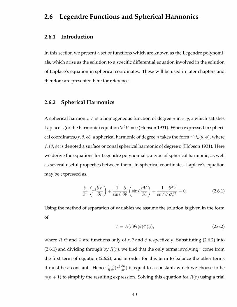
2.6 Legendre Functions and Spherical Harmonics

2.6.1 Introduction

In this section we present a set of functions which are known as the Legendre polynomi-

als, which arise as the solution to a specific differential equation involved in the solution

of Laplace’s equation in spherical coordinates. These will be used in later chapters and

therefore are presented here for reference.

2.6.2 Spherical Harmonics

A spherical harmonic V is a homogeneous function of degree n in x, y, z which satisfies

Laplace’s (or the harmonic) equation ∇2V = 0 (Hobson 1931). When expressed in spheri-

cal coordinates,(r, θ, φ), a spherical harmonic of degree n takes the form rnfn(θ, φ), where

fn(θ, φ) is denoted a surface or zonal spherical harmonic of degree n (Hobson 1931). Here

we derive the equations for Legendre polynomials, a type of spherical harmonic, as well

as several useful properties between them. In spherical coordinates, Laplace’s equation

may be expressed as,

∂

∂r

(

r2∂V

∂r

)

+1

sin θ

∂

∂θ

(

sin θ∂V

∂θ

)

+1

sin2 θ

∂2V

∂φ2= 0. (2.6.1)

Using the method of separation of variables we assume the solution is given in the form

of

V = R(r)Θ(θ)Φ(φ), (2.6.2)

where R,Θ and Φ are functions only of r, θ and φ respectively. Substituting (2.6.2) into

(2.6.1) and dividing through by R(r), we find that the only terms involving r come from

the first term of equation (2.6.2), and in order for this term to balance the other terms

it must be a constant. Hence 1R

ddr

(r2 dRdr

) is equal to a constant, which we choose to be

n(n + 1) to simplify the resulting expression. Solving this equation for R(r) using a trial

40

solution of the form R = rk for some k, we find

R(r) = Arn +Br−n−1, (2.6.3)

where A and B are arbitrary constants. Therefore Laplace’s equation (2.6.1) may be writ-

ten as

n(n+ 1) sin2 θ +sin θ

Θ

d

dθ

(

sin θdΘ

dθ

)

+1

Φ

d2Φ

dφ2= 0. (2.6.4)

Here we can see that the function Φ satisfies the equation 1Φ

d2Φdφ2 = −m2 by the same

argument as used with the r-dependence, where we have chosen the constant to be −m2.

The choice of the negative constant means that, for real m, the solutions are given by

trigonometric functions instead of exponential functions. With this choice of constant we

may solve for the Φ dependence, giving

Φ(φ) = C cos(mφ+D), (2.6.5)

where C and D are two further arbitrary constants. The remaining equation for the θ

dependence of Laplace’s equation is therefore given by,

1

sin θ

d

dθ

(

sin θdΘ

dθ

)

+

(

n(n+ 1) − m2

sin2 θ

)

Θ = 0. (2.6.6)

Equation (2.6.6) may be rewritten by using the substitution cos θ = µ, resulting in what is

known as the associated Legendre differential equation:

d

dµ

(

(1 − µ2)dΘ

dµ

)

+

(

n(n+ 1) − m2

1 − µ2

)

Θ = 0. (2.6.7)

2.6.3 Legendre Polynomials

If there exists symmetry around an axis in the three-dimensional space, we may choose

the coordinate system such that this symmetry axis is aligned with the φ = 0 axis. There-

fore we may remove the φ dependence of the function V , and set m = 0 in the equation

41

(2.6.7). The resulting differential equation is known as Legendre’s differential equation

(Hobson 1931),

d

dµ

(

(1 − µ2)dΘ

dµ

)

+ n(n + 1)Θ = 0, (2.6.8)

and it is shown by Farrell and Ross (1963) that this equation has solutions of the first kind

given by

Θ(µ) = C0

[

1 − n(n+ 1)

2!µ2 +

n(n + 1)(n− 2)(n+ 3)

4!µ4 − . . .

]

+C1

[

µ− (n− 1)(n+ 2)

3!µ3 +

(n− 1)(n+ 2)(n− 3)(n+ 4)

5!µ5 − . . .

]

, (2.6.9)

valid for |µ| < 1 with C0, C1 as arbitrary constants. There are also solutions of a second

kind which converge for |µ| > 1. When n is an integer one of the two sums given in (2.6.9)

terminates at a finite length, and we therefore choose to set the constant in front of the

non-terminating series to be zero, depending on whether n is even or odd, and choose

the other arbitrary constant to be 1.3.5...(2n−1)n!

, which ensures that the finite polynomial

has the value one at µ = 1. These solutions to (2.6.8) with integer n are called Legendre

polynomials and are denoted by Pn(µ), where n is the degree of the polynomial. The first

few Legendre polynomials are given by (MacRobert 1947),

P0(µ) = 1, P1(µ) = µ, P2(µ) =1

2(3µ2 − 1), (2.6.10)

P3(µ) =1

2(5µ3 − 3µ), P4(µ) =

1

8(35µ4 − 30µ2 + 3), (2.6.11)

and are found tabulated in various sources. The nth Legendre polynomial has maximum

degree n and only contains powers of µ which have the same polarity as n. There also

exists the following symmetry in the index n,

Pn(µ) = P−n−1(µ), (2.6.12)

42

resulting from the invariance of (2.6.8) when n is replaced by −(n + 1). Therefore, when

m = 0, the resulting solutions of (2.6.1) are given by

V (r, θ) =∞∑

n=0

(Arn +Br−n−1

)(EPn(µ) + FQn(µ)) , (2.6.13)

whereA,B,E, F are arbitrary coefficients determined by initial and boundary conditions

and Qn(µ) is the nth Legendre function of the second kind, which is not convergent for

|µ| < 1 and hence F = 0 when µ = cos θ. Due to (2.6.12) and the same symmetry in the r

component, we only require the sum to take the positive values of n.

The following expression, known as Rodrigue’s formula, gives a closed form for the

Legendre polynomials (Hobson 1931),

Pn(µ) =1

2nn!

dn

dµn(µ2 − 1)n, (2.6.14)

which is particularly useful for calculating integral relations involving the Legendre

polynomials, and is used in the following derivations.

If we allow n to be a non-integer in the definition (2.6.9), we obtain what are known as

the Legendre functions. These are still denoted Pn(µ), but do not have a closed form

representation, and are defined for all complex n in the form of a hypergeometric series,

as indeed they may be when n is an integer.

2.6.4 Orthogonality and Integral Formulae

The Legendre polynomials form an orthogonal set of functions. This may be derived by

using the Rodrigue’s formula (2.6.14), and the orthogonality property is given by,

∫ 1

−1

Pl(µ)Pn(µ)dµ =2

2n+ 1δln, (2.6.15)

where δln is the Kronecker delta which is one if l = n or zero if l 6= n. An orthonormal set

of polynomials can be created by including the factor√

22n+1

as an additional coefficient

43

in the definition of Pn(µ), though this alters the value of the polynomials at unity as well

as Rodrigue’s formulae and other relations.

The following integral relations are also true for l < n and l ≤ n respectively, which may

be intuitively seen, apart from the constants, by expressing µPl(µ) in terms of a sum of

Legendre polynomials up to degree l + 1 and using (2.6.15),

∫ 1

−1

µPl(µ)Pn(µ)dµ =2n

4n2 − 1δl(n−1). (2.6.16)

∫ 1

−1

µ2Pl(µ)Pn(µ)dµ =4n2 + 4n− 2

(2n− 1)(2n+ 1)(2n+ 3)δln (2.6.17)

+2n(n− 1)

(2n− 3)(2n− 1)(2n+ 1)δl(n−2),

2.6.5 Function Expansion Theorem

As the Legendre polynomials (with integer values of n) are a complete orthogonal set,

any piecewise continuous function may be expressed as a linear combination of the in-

finite set of Legendre polynomials using the following theorem (Whittaker and Watson

1927 cited by Farrell and Ross 1963):

If a function f(x) is bounded on the interval [−1, 1], and continuous except for a finite

number of discontinuities then there exists a series of constant coefficients, Ak, such that

the series∞∑

k=0

AkPk(x), (2.6.18)

converges to f(x) on every point of continuity of f(x) on [−1, 1] and converges on every

discontinuity. The coefficients Ak in this series are determined by the relation,

Ak =2k + 1

2

∫ 1

−1

f(x)Pk(x)dx. (2.6.19)

This relation enables any suitable function to be approximated with a finite number of

44

Legendre polynomials, and therefore the expression in (2.6.13) is a suitably general solu-

tion to the Laplace equation.

2.6.6 Associated Legendre Functions

We now return to (2.6.7) and consider the case when m is a positive integer. We define

the Associated Legendre polynomials as being solutions to (2.6.7) with such a positive

integer m. For each value of n there are 2m+ 1 independent solutions of the first kind of

(2.6.7), given by the following relation (MacRobert 1947),

Pmn (µ) = (−1)m(1 − µ2)

m

2dmPn(µ)

dµm, m = 0, 1, . . . n (2.6.20)

for the positive values of m. The associated Legendre functions for negative integer m

may then be calculated using the relation,

P−mn (µ) = (−1)m (n−m)!

(n+m)!Pm

n (µ). (2.6.21)

It should be noted that the inclusion of the factor (−1)m is a convention which is not fol-

lowed in all definitions of the associated Legendre polynomials. These associated Leg-

endre polynomials are used when the function V has dependence on the third spherical

coordinate, φ, for when the condition of symmetry around an axis is not imposed. They

have a closed form similar to Rodrigue’s formula by combining (2.6.20) with (2.6.14)

which holds for both positive and negative integer values of m and is given by:

Pmn (µ) =

1

2nn!(1 − µ2)

m

2dm+n[(µ2 − 1)n]

dµm+n. (2.6.22)

Note that, for odd values of m, the associated Legendre polynomial is not a polyno-

mial due to the presence of the square root in (2.6.20) and (2.6.22), despite what the name

would suggest. However, they are still commonly denoted the associated Legendre poly-

nomials for integer values of n and m, with |m| ≤ n. The first few such functions are

45

given by

P 00 (µ) = 1, (2.6.23)

P−11 (µ) =

1

2

√

1 − µ2, P 01 (µ) = µ, P 1

1 (µ) = −√

1 − µ2 (2.6.24)

The associated Legendre polynomials are also orthogonal with respect to n over [−1, 1],

with the following orthogonality relation including the constants,

∫ 1

−1

Pml (µ)Pm

n (µ)dµ =2

2n+ 1

(n +m)!

(n−m)!δln. (2.6.25)

The surface harmonics mentioned in (2.6.2) are given by,

Y mn (θ, φ) = Pm

n (cos θ)eimφ, (2.6.26)

and the general solution to Laplace’s equation when the axial symmetry is not imposed,

(2.6.1), may be written as,

V (r, θ, φ) =∞∑

n=0

n∑

m=−n

(Arn +Br−n−1

)(C cosmφ+D sinmφ) (EPm

n (µ) + FQmn (µ)) ,

(2.6.27)

subject to suitable boundary conditions to determine the six arbitrary constants.

46

Chapter 3

Non-Uniform Inflation of a Cylindrical

Membrane

3.1 Introduction

In this chapter we consider a cylindrical, hyperelastic, isotropic, incompressible mem-

brane, subject to a constant internal pressure. This boundary value problem has been

studied by many authors as a classical problem of solid mechanics. Adkins and Rivlin

(1952), Green and Adkins (1960) and Kydoniefs (1969) all consider this, whilst requiring

the tube to remain cylindrical under the deformation. A connected bifurcation analy-

sis considers whether or not multiple configurations of the deformed tube can exist for

a given set of boundary conditions and internal pressure. Of particular interest are lo-

cally bulging solutions, where there exists an enlarged section of the tube connected to

uniformly inflated sections away from the local bulge, in a similar manner to soliton so-

lutions in wave propagation. The biological motivation behind interest in these solutions

is the study of aneurysms found in blood vessels; such a local bulge causes a lowering

of the blood pressure, blood stagnation and potential rupture, with serious medical com-

plications.

47

In this chapter we consider the conditions on the strain-energy function of the material of

the tube required in order for such bulging or necking solutions to exist. Chapter 4 will

then study the stability of such solutions. Throughout these two chapters the examples

will be mostly given for the Gent strain-energy function (2.2.13). Chapter 5 will then

compare a range of strain-energy functions.

3.2 Literature Review

3.2.1 Experimental Studies

The inflation of a thin-walled rubber tube via control of the internal volume or pressure

has been considered experimentally by a range of authors, often entwined with analyti-

cal or numerical results. In the experiments of Kyriakides and Chang (1990), which are

pressure controlled using compressed air, the tube inflates cylindrically until a limiting

pressure is reached, and these experiments are shown in Figure 3.2.1. After this limiting

pressure is reached a bulge forms at one point of the tube with a decrease in the radius

elsewhere. Further inflation causes the diameter to expand before reaching a maximum

size, at which point the bulge begins to spread laterally along the tube at a constant prop-

agation pressure. After the bulge has filled the tube the inflation continues in a uniform

manner, with an increasing pressure. While the non-uniformity is localised in this way,

the remainder of the tube remains uniform. In Kyriakides and Chang (1991), the defor-

mation is volume controlled by filling the tube with water, resulting in similar behaviour

as described for the pressure controlled case. These experiments are consistent with those

described by Alexander (1971).

When an ordinary cylindrical rubber party balloon is inflated these features may be ob-

served, particularly the state in which two uniform sections of different radii are joined

by a non-uniform section. Due to comparisons with various phenomena observed in

other problems which will be discussed later, this behaviour will be called the kinked state

48

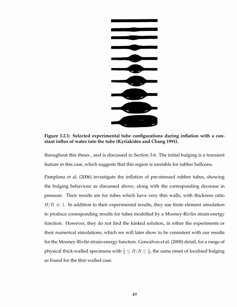
Figure 3.2.1: Selected experimental tube configurations during inflation with a con-stant influx of water into the tube (Kyriakides and Chang 1991).

throughout this thesis , and is discussed in Section 3.6. The initial bulging is a transient

feature in this case, which suggests that this region is unstable for rubber balloons.

Pamplona et al. (2006) investigate the inflation of pre-stressed rubber tubes, showing

the bulging behaviour as discussed above, along with the corresponding decrease in

pressure. Their results are for tubes which have very thin walls, with thickness ratio

H/R ≪ 1. In addition to their experimental results, they use finite element simulation

to produce corresponding results for tubes modelled by a Mooney-Rivlin strain-energy

function. However, they do not find the kinked solution, in either the experiments or

their numerical simulations, which we will later show to be consistent with our results

for the Mooney-Rivlin strain-energy function. Goncalves et al. (2008) detail, for a range of

physical thick-walled specimens with 14≤ H/R ≤ 1

2, the same onset of localised bulging

as found for the thin walled case.

49

3.2.2 Analytical Studies

Alexander (1971) considered the uniform inflation of the tube, using both linear elastic-

ity and a specific nonlinear strain-energy function which has not been used in further

studies. They found the relationship between the pressure and the inflated radius for

these two cases. However, they assumed that the localised bulging found experimen-

tally was caused by material or geometric variations and not as a consequence of the

non-monotonic pressure-volume curve. They found that the linear theory incorrectly

predicts that the axial load has no dependence on this deformation, and show that the

limiting pressure at which localised bulging occurs varies with the value of the axial load

for their strain-energy function. Benedict et al. (1979) extend this work to include a non-

zero axial force, and present a numerical scheme for finding the limiting pressure in this

case, as well as the case of prescribed elongation. However, they do not consider what

happens after the limiting pressure, including any description of the bulged state.

Pipkin (1968) shows, in an extremely concise way, that both of the equations of equilib-

rium for an axisymmetric cylindrical membrane may be integrated, provided the mem-

brane is isotropic and a strain-energy function exists. This is a very useful result as it

reduces the order of the differential equations by one.

Yin (1977) presents an analytical study in which he, using parallels with the inflation of

spherical balloons, makes some assumptions on the form of the strain-energy function

in order to consider the propagating solution found experimentally. Yin (1977) finds that

such a solution has a lower energy than a uniform tube with the same internal pressure,

and therefore it is the energy-minimising configuration, assuming the internal pressure

is from an isothermic gas. Details are given of a method for determining the properties

of the strain-energy function from experimental results for a particular material sample.

The very large deformations which occur during the inflation process make it particu-

larly attractive to determine the behaviour of the strain-energy function at high strain

using this technique.

50

Haughton and Ogden (1979a) consider bifurcations in both the case where the bifur-

cated mode remains axisymmetric, and also prismatic modes where the tube deforms to

a non-axisymmetric shape throughout the tube. Haughton and Ogden (1979a) present a

bifurcation condition on the general separable strain-energy function of the type given

in (2.2.14) for the nth prismatic mode to exist, that is at least one of the exponents α has

an absolute value less than unity. In the following sections it will be shown that this

condition, when evaluated for bifurcation into the zeroth mode, gives the condition for

axisymmetric bifurcated modes which are non-uniform in the axial direction, as we are

interested in. However, in Haughton and Ogden (1979a) this condition was discarded

as the linear eigenfunction for the zeroth mode predicts a constant, whereas in fact a

non-constant function exists for the nonlinear equation. They do correctly state that the

bifurcation, if it exists, occurs before the pressure maximum, for the case of an infinite

tube with fixed axial stretch. They do not consider the case of closed ends, which shall

be discussed here.

Chater and Hutchinson (1984) show that the propagating solution exists whenever the

pressure-volume curve for uniform inflation has a Maxwell construction; that is a value

of the pressure such that two distinct areas bounded between the curve and the straight

line have equal area. The existence of such a Maxwell line is guaranteed when the

pressure-volume curve has a local, but not global, maximum followed by a minimum.

Chater and Hutchinson (1984) point out the similarities of this deformation with propa-

gating buckles in metal tubes (Kyriakides and Babcock 1981), propagating necks in mate-

rials under tension (Hutchinson and Neale 1983), and phase transitions in bars (Ericksen

1975). They also state that a characteristic of such behaviour is the high pressure required

to enter the bifurcated mode, followed by a much lower value required once the mode

has been initiated. This characteristic is seen in the previously cited studies as well as in

the experiments by Kyriakides and Chang (1990).

Kyriakides and Chang (1991) solve the differential equations for the membrane tube nu-

merically for various strain-energy functions, and find good agreement with their exper-

imental results, where the ratio of thickness to radius for the rubber tubes involved was

51

approximately one quarter.

Gent (2005) and Kanner and Horgan (2007) discuss how the form of the strain-energy

function which models a closed tube affects whether a limit-point instability exists, after

which localised bulges occur. They show how these instabilities exist at the maximum of

the pressure-volume curve belonging to the inflated cylindrical tube.

Haughton (2001) derives the bifurcation condition and provides examples of the bulged

configuration for the Varga strain-energy function in a tube with no axial stretch. Here

we shall expand this for general strain-energy functions, closed or open ended tubes and

any value of axial stretch.

3.3 Inflation of a Cylindrical Tube

3.3.1 Governing Equations

We develop a description of the elastic deformation of such a tube for a general isotropic,

incompressible strain-energy function, which may be validated by the experimental re-

sults conducted on rubber detailed above. We are then interested in the response of non-

rubberlike strain-energy functions, particularly those which are appropriate to biological

materials.

The analysis considered here is for an incompressible, isotropic, hyperelastic membrane

tube. We consider only axially symmetric deformations from the originally axially sym-

metric configuration. For prismatic deformations we refer to Haughton and Ogden

(1979a). In the reference configuration the tube is assumed to have uniform radius R,

uniform thickness H and is described by coordinates 0 ≤ Θ ≤ 2π,−∞ ≤ Z ≤ ∞. The

position vector X is given by X = ReR(Θ) + ZeZ . When inflated by a constant inter-

nal pressure, P , it is assumed that the inflated configuration maintains axial symmetry

and the radius may be constant or vary along the axial direction. We assume that in the

undeformed tube the thickness is much smaller than the radius, H ≪ R, and we only

52

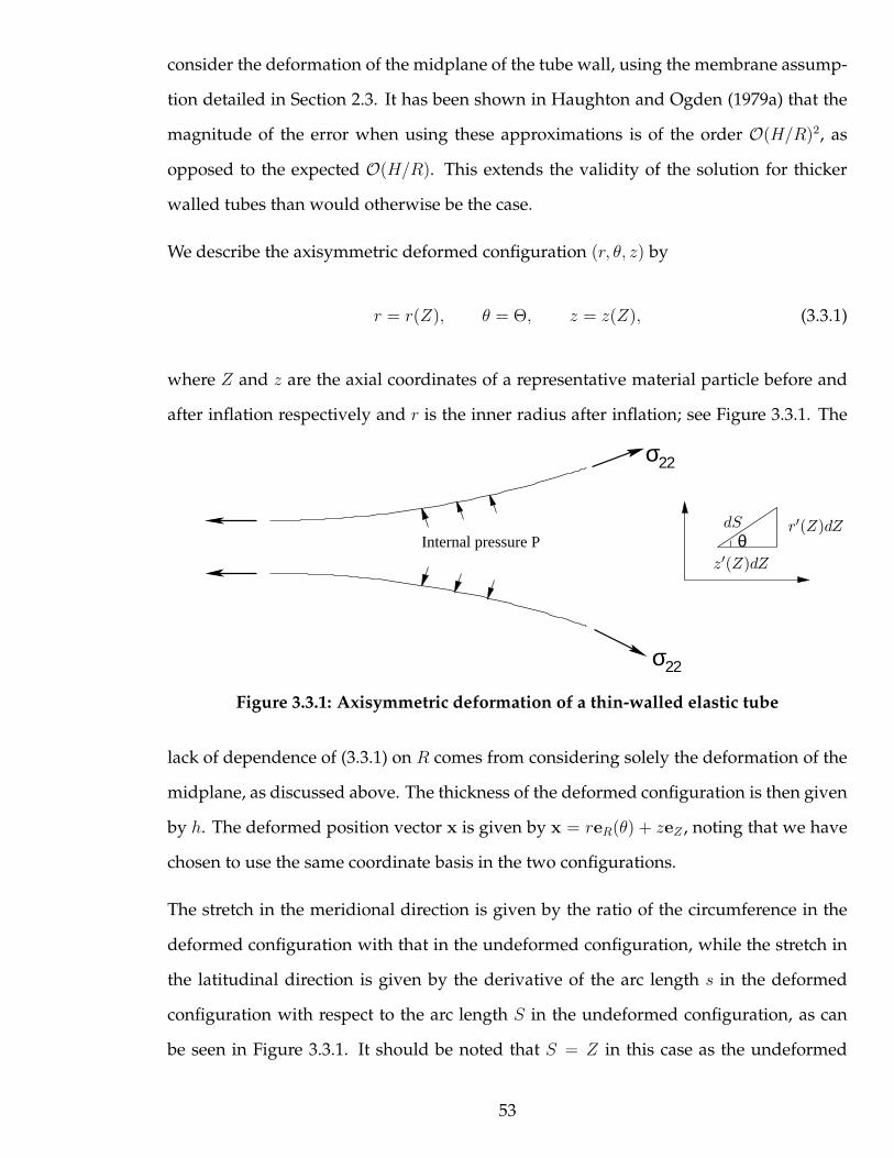
consider the deformation of the midplane of the tube wall, using the membrane assump-

tion detailed in Section 2.3. It has been shown in Haughton and Ogden (1979a) that the

magnitude of the error when using these approximations is of the order O(H/R)2, as

opposed to the expected O(H/R). This extends the validity of the solution for thicker

walled tubes than would otherwise be the case.

We describe the axisymmetric deformed configuration (r, θ, z) by

r = r(Z), θ = Θ, z = z(Z), (3.3.1)

where Z and z are the axial coordinates of a representative material particle before and

after inflation respectively and r is the inner radius after inflation; see Figure 3.3.1. The

θInternal pressure P

σ22

σ22

dS

z′(Z)dZ

r′(Z)dZ

Figure 3.3.1: Axisymmetric deformation of a thin-walled elastic tube

lack of dependence of (3.3.1) on R comes from considering solely the deformation of the

midplane, as discussed above. The thickness of the deformed configuration is then given

by h. The deformed position vector x is given by x = reR(θ) + zeZ , noting that we have

chosen to use the same coordinate basis in the two configurations.

The stretch in the meridional direction is given by the ratio of the circumference in the

deformed configuration with that in the undeformed configuration, while the stretch in

the latitudinal direction is given by the derivative of the arc length s in the deformed

configuration with respect to the arc length S in the undeformed configuration, as can

be seen in Figure 3.3.1. It should be noted that S = Z in this case as the undeformed

53

configuration is a tube with constant radius R. From Figure 3.3.1 we can see that this can

be written as:

λθ =2πr

2πR, λz =

ds

dS=

ds

dZ, λr =

h

H. (3.3.2)

Since the deformation is axially symmetric, the principal directions of stretch coincide

with the lines of latitude, the meridian and the normal to the deformed surface. Thus,

the principal stretches are given by

λ1 =r

R, λ2 = (r′2 + z′2)

12 , λ3 =

h

H, (3.3.3)

where we use the indices (1, 2, 3) for the latitudinal, meridional and normal directions

respectively and the primes indicate differentiation with respect to Z. Clearly, these

three directions are mutually orthogonal, and are therefore the principal directions of

the deformation. Thus the principal Cauchy stresses in the deformed configuration for

an incompressible material are given by

σi = λiWi − p, i = 1, 2, 3, (3.3.4)

where W = W (λ1, λ2, λ3) is the strain-energy function, Wi = ∂W/∂λi and p is the La-

grange multiplier associated with the constraint of incompressibility. Utilising the in-

compressibility constraint, λ1λ2λ3 = 1, and the membrane assumption of no stress in the

thickness direction, σ3 = 0, equation (3.3.4) becomes

σi = λiWi, i = 1, 2, (3.3.5)

where W (λ1, λ2) = W (λ1, λ2, λ−11 λ−1

2 ) and Wi = ∂W /∂λi (Ogden 1997).

Considering the balance of forces in an infinitesimal section of the material formed by

cutting the tube twice perpendicular to the Z-axis, we find that

r(σ2h)′ + hr′(σ2 − σ1) = 0. (3.3.6)

54

Similarly, by considering equilibrium in the normal direction of a small volume element,

σ2(r′′z′ − r′z′′)

λ32

− z′σ1

rλ2+P ∗

λ3= 0, (3.3.7)

where P ∗ = P/H . We will discuss later how these two equations may be derived from

the equilibrium equations given in (2.1.41). Using (3.3.6) to express σ1 as σ1 = (hrσ2)′

hr′,

(3.3.7) is a first order differential equation for σ2 which may be solved via an integrating

factor leading to,

σ2z′

λ22

− 1

2P ∗λ2

1R = C2, (3.3.8)

where C2 is a constant. This equation could be derived immediately by considering the

resultant from balancing forces acting through the tube in the Z-direction, and exists

even when R or H are non-constant functions of Z. However, it does require that the

internal pressure P is not a function of Z, and therefore it is not appropriate in the case

of tubes which are partially filled with a liquid, such as those considered by Pamplona

et al. (2001). It was shown by Pipkin (1968) that there exists a second integral of the

axisymmetric elastic tube provided that a strain-energy function exists as in (3.3.5). In

this case, with H and R both being constant, (3.3.6) becomes

λ2(W2)′ =

r′

RW1. (3.3.9)

Then, using W ′ = λ′1W1 + λ′2W2 and λ′1 = r′/R, this leads to,

W ′ = (λ2W2)′, (3.3.10)

which may then be integrated to give the second integral described by Pipkin (1968). Our

two integrals of the equilibrium equations may therefore be given by,

W − λ2W2 = C1, (3.3.11)

W2z′

λ2− 1

2P ∗λ2

1R = C2, (3.3.12)

55

where C1, C2 are constants. These two integrals are the result of symmetries in the vari-

ational form of the current deformation, with the second integral only existing when R

and H are both constant, as mentioned above. Equations (3.3.11) and (3.3.12) are equiv-

alent to equations (3.27) and (3.29) of Haughton (2001) respectively, which are derived

from a more elaborate thin-shell theory considering the deformation of the midplane of

a shell with negligible thickness. For more details on the derivation of the above results,

including the asymptotic estimates from neglecting the small thickness which are also

relevant to these results, see Haughton and Ogden (1979a) and Haughton and Ogden

(1979b).

Epstein and Johnston (2001) give an alternative, equivalent, self-contained derivation of

the equations of motion using a force-balance technique, which in our notation may be

written as,[

Rσ2z′

λ22

]′

− P ∗ rr′ = ρz,

[

Rσ2r′

λ22

]′

− σ1

λ1

+ P ∗ rz′ = ρr, (3.3.13)

where ρ is the material density and a superimposed dot denotes differentiation with re-

spect to t. It is possible to derive (3.3.13) via a perturbation expansion of the full equations

of motion, (2.1.41), between two axisymmetric cylindrical coordinate systems (R, θ, Z)

and (r, θ, z), and we will outline this here. Taking (2.1.41) as the starting point, which in-

volves derivatives with respect to bothR and Z, we first non-dimensionalise with respect

to the inner radius Ri and the infinitesimal shear modulus µ. We introduce a dimension-

less thickness coordinate η through R = Ri + Hη, 0 < η < 1, which we use instead of

R. Taking a regular perturbation expansion in ǫ = H/Ri of the quantities r, z, P and σ,

we then find, to first order in ǫ, the equations given in (3.3.13), along with the fact that

the pressure P must be of order ǫ. Full details of this procedure may be found in Er-

bay and Demiray (1995) for a neo-Hookean strain-energy function and Tuzel and Erbay

(2004) for any strain-energy function. We also note that these two studies, along with

Kydoniefs and Spencer (1987) which also carries out the above asymptotic expansion for

a particular problem, include the possibility of a tangential traction acting on the inner

surface of the deformed membrane as well as the normal pressure. In Chapter 4 we show

56

that the static version of (3.3.13) may be derived via an energy minimisation approach;

the dynamic equations (3.3.13) are derived in Chen (1997) using such an energy minimi-

sation approach.

Equation (3.3.13) can be shown to be equivalent to equations (3.3.6) and (3.3.7) when

static deformations are considered, although they represent the force balances in the z

and r directions rather than in the tangential and normal directions respectively, which

are given by (r′er + z′ez)/λ2 and (z′er − r′ez)/λ2 respectively.

To non-dimensionalise the problem all the length variables are rescaled by the original

radius R, or equivalently R is set to be unity. Similarly, we divide the strain-energy func-

tion W , and the pressure P ∗, by the infinitesimal shear modulus µ to non-dimensionalise

the stresses.

3.3.2 Conditions at Infinity

In this work we are interested in localised bulging or necking solutions in which the tube

has a constant radius r∞ and constant axial stretch z∞ far away from the localised bulge

or neck if one exists. Hence we impose the following conditions a priori,

limZ→∞

r(Z) = r∞R, limZ→∞

z(Z) = z∞Z, (3.3.14)

and hence

r′ → 0, z′ → z∞, λ1 → r∞, λ2 → z∞ as Z → ±∞. (3.3.15)

Essentially we are imposing a pre-stress on the material, associated with the pressure P

through r∞ and z∞, and then determining whether there exist other non-uniform states

which satisfy the governing equations but decay to the same constant radius and axial

stretch at infinity.

We can find the constants C1 and C2 by evaluating (3.3.11) and (3.3.12) in the limit Z →

57

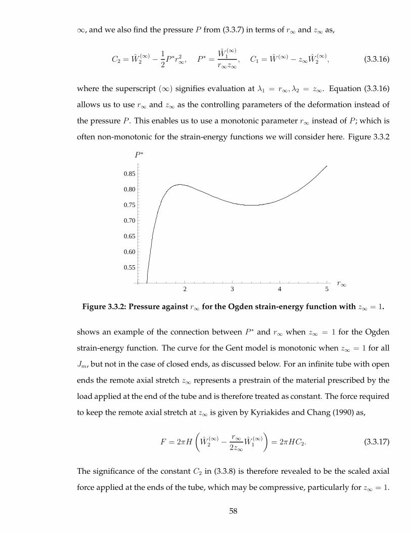
∞, and we also find the pressure P from (3.3.7) in terms of r∞ and z∞ as,

C2 = W(∞)2 − 1

2P ∗r2

∞, P ∗ =W

(∞)1

r∞z∞, C1 = W (∞) − z∞W

(∞)2 , (3.3.16)

where the superscript (∞) signifies evaluation at λ1 = r∞, λ2 = z∞. Equation (3.3.16)

allows us to use r∞ and z∞ as the controlling parameters of the deformation instead of

the pressure P . This enables us to use a monotonic parameter r∞ instead of P ; which is

often non-monotonic for the strain-energy functions we will consider here. Figure 3.3.2

2 3 4 5

0.55

0.60

0.65

0.70

0.75

0.80

0.85

r∞

P ∗

Figure 3.3.2: Pressure against r∞ for the Ogden strain-energy function with z∞ = 1.

shows an example of the connection between P ∗ and r∞ when z∞ = 1 for the Ogden

strain-energy function. The curve for the Gent model is monotonic when z∞ = 1 for all

Jm, but not in the case of closed ends, as discussed below. For an infinite tube with open

ends the remote axial stretch z∞ represents a prestrain of the material prescribed by the

load applied at the end of the tube and is therefore treated as constant. The force required

to keep the remote axial stretch at z∞ is given by Kyriakides and Chang (1990) as,

F = 2πH

(

W(∞)2 − r∞

2z∞W

(∞)1

)

= 2πHC2. (3.3.17)

The significance of the constant C2 in (3.3.8) is therefore revealed to be the scaled axial

force applied at the ends of the tube, which may be compressive, particularly for z∞ = 1.

58

Naturally this depends on the value of r∞ as well as the strain-energy function. For

human arteries Learoyd and Taylor (1966) give the axial stretch as 1.28 to 1.67 for people

under 35, and 1.14 to 1.32 for people over 35, while Humphrey et al. (2009) states that it

is of the order z∞ ≈ 1.5 for various mammals.

For a tube with closed ends and no axial loading, where we assume the ends are suitably

far away from the localised bulge or neck that we may still consider the tube to be infinite,

we require that the force balance in the Z direction is zero, from which we can derive the

condition C2 = 0. For closed ends with no axial loading, we find the following relation

from (3.3.12),

r∞W1(r∞, z∞) = 2z∞W2(r∞, z∞), (3.3.18)

which can be used to determine z∞ for any given r∞. The relation given in (3.3.18) may

have multiple branches, that is multiple values of z∞ which satisfy (3.3.18) for a given r∞.

In this case, we need to choose the branch which passes through the undeformed solution

r∞ = 1, z∞ = 1, which is always a solution to (3.3.18) for any admissible strain-energy

function W which satisfying the conditions given in (2.2.6).

The closed ends relation (3.3.18) for the Varga and Gent strain-energy function given by

(2.2.10) and (2.2.13) become respectively,

1 + r2∞z∞ − 2r∞z

2∞ = 0, 1 + r4

∞z2∞ − 2r2

∞z4∞ = 0, (3.3.19)

which may be solved explicitly for z∞ and are plotted in Figure 3.3.3. It should be noted

that the condition for the Gent strain-energy function (2.2.13) is independent of Jm and in

fact corresponds to the relation for the neo-Hookean strain-energy function. This second

relation also holds for any other strain-energy functions which are solely a function of I1,

such as the LSS and Fung strain-energy functions. In addition, the first relation also holds

for any function which is solely a function of i1 as given in (2.1.54). A similar relation

can be found for a strain-energy function which only depends on I2 or i2 for example,

although no such relation may be found for the Ogden strain-energy function given by

(2.2.14) as it is expressed as a function of the stretches rather than a single invariant.

59

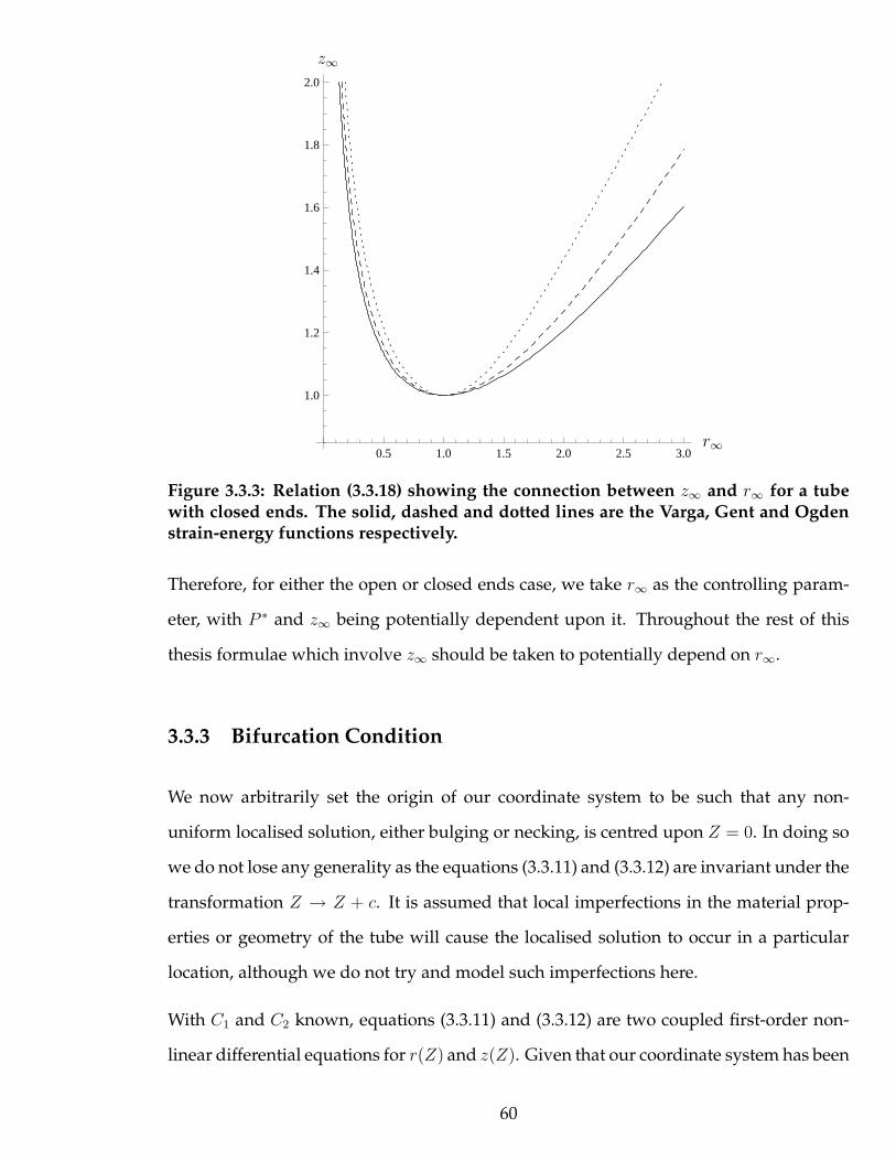
0.5 1.0 1.5 2.0 2.5 3.0

1.0

1.2

1.4

1.6

1.8

2.0

r∞

z∞

Figure 3.3.3: Relation (3.3.18) showing the connection between z∞ and r∞ for a tubewith closed ends. The solid, dashed and dotted lines are the Varga, Gent and Ogdenstrain-energy functions respectively.

Therefore, for either the open or closed ends case, we take r∞ as the controlling param-

eter, with P ∗ and z∞ being potentially dependent upon it. Throughout the rest of this

thesis formulae which involve z∞ should be taken to potentially depend on r∞.

3.3.3 Bifurcation Condition

We now arbitrarily set the origin of our coordinate system to be such that any non-

uniform localised solution, either bulging or necking, is centred upon Z = 0. In doing so

we do not lose any generality as the equations (3.3.11) and (3.3.12) are invariant under the

transformation Z → Z + c. It is assumed that local imperfections in the material prop-

erties or geometry of the tube will cause the localised solution to occur in a particular

location, although we do not try and model such imperfections here.

With C1 and C2 known, equations (3.3.11) and (3.3.12) are two coupled first-order non-

linear differential equations for r(Z) and z(Z). Given that our coordinate system has been

60

set arbitrarily, the axial symmetry of the entire deformation together with the symmetry

in the end conditions (3.3.15), we focus only on solutions which are symmetric about the

origin Z = 0. The required conditions are therefore,

r′(0) = 0, z(0) = 0. (3.3.20)

To find the corresponding value r(0) for a given r∞, if one exists, (3.3.12) and (3.3.11) are

evaluated at Z = 0, obtaining respectively,

W2(r0, z′0) −

W(∞)1

2r∞z∞(r2

0 − r2∞) − W

(∞)2 = 0, (3.3.21)

W (r0, z′0) − z′0 W2(r0, z

′0) − W (∞) + z∞W

(∞)2 = 0, (3.3.22)

where r0 = r(0), z′0 = z′(0), and both are required to be positive for physical defor-

mations. In theory these two equations can be solved to find r0 and z′0 as functions of

r∞, though for most strain-energy functions this process must be numerical. Obviously,

r0 = r∞ and z′0 = z∞ is always a solution of (3.3.21) and (3.3.22) corresponding to the

trivial uniform solution r(Z) ≡ r∞. A necessary condition for a non-uniform bifurcated

solution to exist is therefore that (3.3.21) and (3.3.22) have a solution other than r0 = r∞,

z′0 = z∞.

Suppose that after the trivial solution r0 = r∞ has been factorised out, the solution is

given by

r0 = q(r∞), (3.3.23)

for some unknown function q. Any bifurcation values are therefore given by the roots

of r∞ = q(r∞); the intersection of the trivial solution with the nontrivial solutions. It

should be noted that the existence of such a non-trivial value of r0 does not guarantee

that it corresponds to a localised solution of r(Z), or even a finite solution. In particular,

it must be verified that z′0 > 0 to ensure that the solution is physical. Section 5.2 details

this process for the Varga strain-energy function as an illustration of this method, and

may be read as an example before continuing here.

61

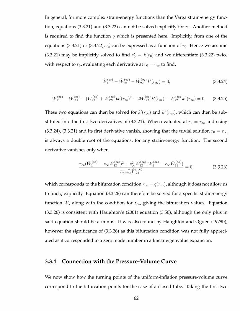
In general, for more complex strain-energy functions than the Varga strain-energy func-

tion, equations (3.3.21) and (3.3.22) can not be solved explicitly for r0. Another method

is required to find the function q which is presented here. Implicitly, from one of the

equations (3.3.21) or (3.3.22), z′0 can be expressed as a function of r0. Hence we assume

(3.3.21) may be implicitly solved to find z′0 = k(r0) and we differentiate (3.3.22) twice

with respect to r0, evaluating each derivative at r0 = r∞ to find,

W(∞)1 − W

(∞)12 − W

(∞)22 k′(r∞) = 0, (3.3.24)

W(∞)11 − W

(∞)112 − (W

(∞)22 + W

(∞)222 )k′(r∞)2 − 2W

(∞)122 k′(r∞) − W

(∞)22 k′′(r∞) = 0. (3.3.25)

These two equations can then be solved for k′(r∞) and k′′(r∞), which can then be sub-

stituted into the first two derivatives of (3.3.21). When evaluated at r0 = r∞ and using

(3.3.24), (3.3.21) and its first derivative vanish, showing that the trivial solution r0 = r∞

is always a double root of the equations, for any strain-energy function. The second

derivative vanishes only when

r∞(W(∞)1 − z∞W

(∞)12 )2 + z2

∞W(∞)22 (W

(∞)1 − r∞W

(∞)11 )

r∞z2∞W

(∞)22

= 0, (3.3.26)

which corresponds to the bifurcation condition r∞ = q(r∞), although it does not allow us

to find q explicitly. Equation (3.3.26) can therefore be solved for a specific strain-energy

function W , along with the condition for z∞, giving the bifurcation values. Equation

(3.3.26) is consistent with Haughton’s (2001) equation (3.50), although the only plus in

said equation should be a minus. It was also found by Haughton and Ogden (1979b),

however the significance of (3.3.26) as this bifurcation condition was not fully appreci-

ated as it corresponded to a zero mode number in a linear eigenvalue expansion.

3.3.4 Connection with the Pressure-Volume Curve

We now show how the turning points of the uniform-inflation pressure-volume curve

correspond to the bifurcation points for the case of a closed tube. Taking the first two

62

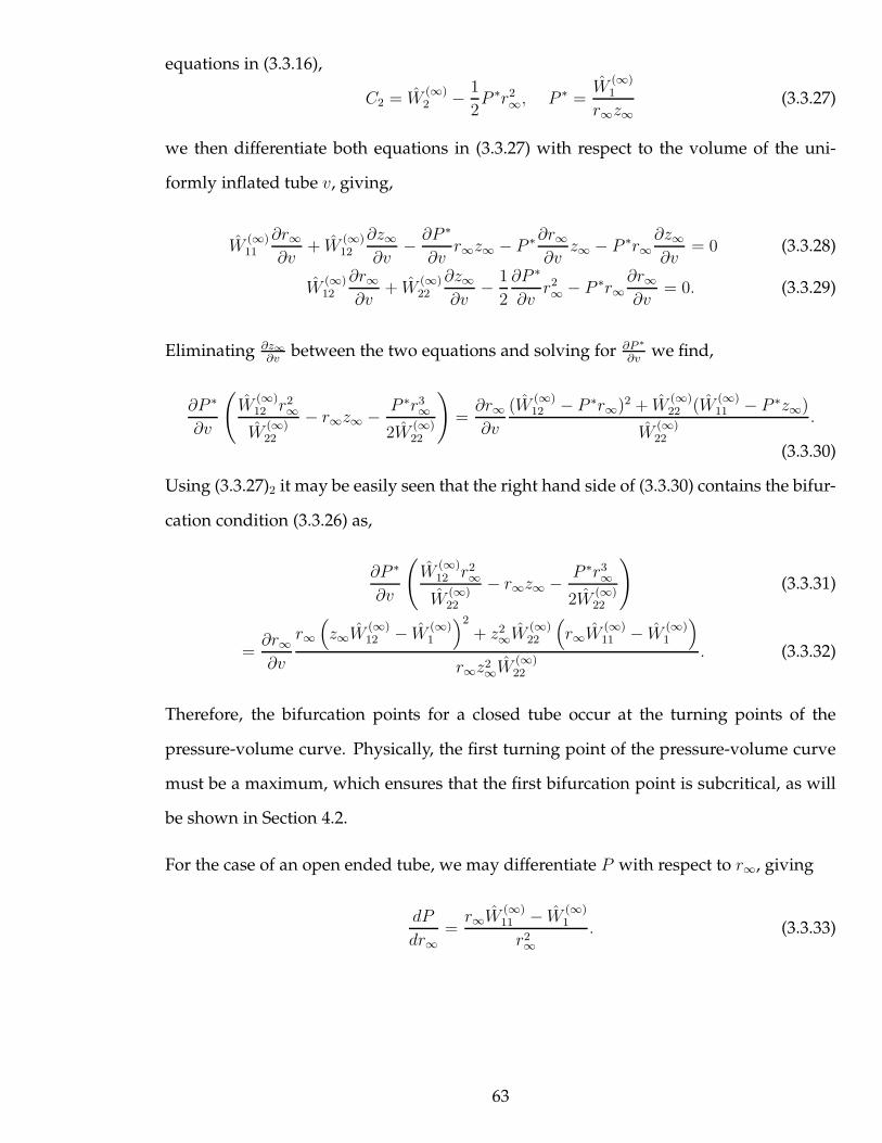
equations in (3.3.16),

C2 = W(∞)2 − 1

2P ∗r2

∞, P ∗ =W

(∞)1

r∞z∞(3.3.27)

we then differentiate both equations in (3.3.27) with respect to the volume of the uni-

formly inflated tube v, giving,

W(∞)11

∂r∞∂v

+ W(∞)12

∂z∞∂v

− ∂P ∗

∂vr∞z∞ − P ∗∂r∞

∂vz∞ − P ∗r∞

∂z∞∂v

= 0 (3.3.28)

W(∞)12

∂r∞∂v

+ W(∞)22

∂z∞∂v

− 1

2

∂P ∗

∂vr2∞ − P ∗r∞

∂r∞∂v

= 0. (3.3.29)

Eliminating ∂z∞∂v

between the two equations and solving for ∂P ∗

∂vwe find,

∂P ∗

∂v

(

W(∞)12 r2

∞

W(∞)22

− r∞z∞ − P ∗r3∞

2W(∞)22

)

=∂r∞∂v

(W(∞)12 − P ∗r∞)2 + W

(∞)22 (W

(∞)11 − P ∗z∞)

W(∞)22

.

(3.3.30)

Using (3.3.27)2 it may be easily seen that the right hand side of (3.3.30) contains the bifur-

cation condition (3.3.26) as,

∂P ∗

∂v

(

W(∞)12 r2

∞

W(∞)22

− r∞z∞ − P ∗r3∞

2W(∞)22

)

(3.3.31)

=∂r∞∂v

r∞

(

z∞W(∞)12 − W

(∞)1

)2

+ z2∞W

(∞)22

(

r∞W(∞)11 − W

(∞)1

)

r∞z2∞W

(∞)22

. (3.3.32)

Therefore, the bifurcation points for a closed tube occur at the turning points of the

pressure-volume curve. Physically, the first turning point of the pressure-volume curve

must be a maximum, which ensures that the first bifurcation point is subcritical, as will

be shown in Section 4.2.

For the case of an open ended tube, we may differentiate P with respect to r∞, giving

dP

dr∞=r∞W

(∞)11 − W

(∞)1

r2∞

. (3.3.33)

63

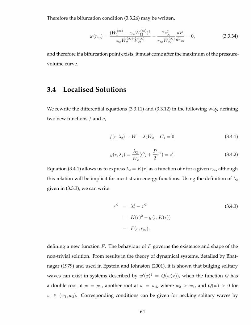
Therefore the bifurcation condition (3.3.26) may be written,

ω(r∞) =(W

(∞)1 − z∞W

(∞)12 )2

z∞W(∞)2 W

(∞)22

− 2z2∞

r∞W(∞)22

dP

dr∞= 0, (3.3.34)

and therefore if a bifurcation point exists, it must come after the maximum of the pressure-

volume curve.

3.4 Localised Solutions

We rewrite the differential equations (3.3.11) and (3.3.12) in the following way, defining

two new functions f and g,

f(r, λ2) ≡ W − λ2W2 − C1 = 0, (3.4.1)

g(r, λ2) ≡λ2

W2

(C2 +P

2r2) = z′. (3.4.2)

Equation (3.4.1) allows us to express λ2 = K(r) as a function of r for a given r∞, although

this relation will be implicit for most strain-energy functions. Using the definition of λ2

given in (3.3.3), we can write

r′2 = λ22 − z′2 (3.4.3)

= K(r)2 − g (r,K(r))

= F (r; r∞),

defining a new function F . The behaviour of F governs the existence and shape of the

non-trivial solution. From results in the theory of dynamical systems, detailed by Bhat-

nagar (1979) and used in Epstein and Johnston (2001), it is shown that bulging solitary

waves can exist in systems described by w′(x)2 = Q(w(x)), when the function Q has

a double root at w = w1, another root at w = w2, where w2 > w1, and Q(w) > 0 for

w ∈ (w1, w2). Corresponding conditions can be given for necking solitary waves by

64

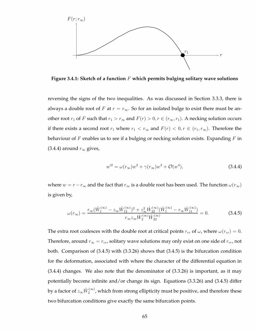
r

F (r; r∞)

r1

Figure 3.4.1: Sketch of a function F which permits bulging solitary wave solutions

reversing the signs of the two inequalities. As was discussed in Section 3.3.3, there is

always a double root of F at r = r∞. So for an isolated bulge to exist there must be an-

other root r1 of F such that r1 > r∞ and F (r) > 0, r ∈ (r∞, r1). A necking solution occurs

if there exists a second root r1 where r1 < r∞ and F (r) < 0, r ∈ (r1, r∞). Therefore the

behaviour of F enables us to see if a bulging or necking solution exists. Expanding F in

(3.4.4) around r∞ gives,

w′2 = ω(r∞)w2 + γ(r∞)w3 + O(w4), (3.4.4)

where w = r− r∞ and the fact that r∞ is a double root has been used. The function ω(r∞)

is given by,

ω(r∞) =r∞(W

(∞)1 − z∞W

(∞)12 )2 + z2

∞W(∞)22 (W

(∞)1 − r∞W

(∞)11 )

r∞z∞W(∞)2 W

(∞)22

= 0. (3.4.5)

The extra root coalesces with the double root at critical points rcr of ω, where ω(rcr) = 0.

Therefore, around r∞ = rcr, solitary wave solutions may only exist on one side of rcr, not

both. Comparison of (3.4.5) with (3.3.26) shows that (3.4.5) is the bifurcation condition

for the deformation, associated with where the character of the differential equation in

(3.4.4) changes. We also note that the denominator of (3.3.26) is important, as it may

potentially become infinite and/or change its sign. Equations (3.3.26) and (3.4.5) differ

by a factor of z∞W(∞)2 , which from strong ellipticity must be positive, and therefore these

two bifurcation conditions give exactly the same bifurcation points.

65

3.4.1 Near-Critical Solutions

We now show that solitary wave solutions do exist on one side of rcr without evaluating

F by looking for near-critical solutions of (3.4.4), where r∞ is close to rcr and we define

ǫ = r∞ − rcr which may be positive or negative. Expanding around rcr we obtain

w′2 = ω′(rcr)ǫw2 + γ(rcr)w

3 + O(w4), (3.4.6)

where O(ǫw2) = O(w3). Naturally w′ may only change sign when the right hand side

of (3.4.6) is zero, where w = −ω′(rcr)ǫγ(rcr)

. On the assumption that w′ ≡ r′ does not change

sign, then when r0 > r∞, a bulging solution exists with w′ < 0 and w > 0; whereas when

r0 < r∞, a necking solution exists with w′ > 0 and w < 0. Thus in both cases the square

root may be taken in (3.4.6) to give,

w′ = −w√

ω′(rcr)ǫ+ γ(rcr)w. (3.4.7)

This equation is naturally related to the following four equations:

w′1 = −aw1

√

1 + bw1, w′2 = −aw2

√

1 − bw2,

w′3 = −aw3

√

−1 + bw3, w′4 = −aw4

√

−1 − bw4,

where w1, w2, w3, w4 are functions of Z and a, b are positive constants given by

a =√

|ω′(rcr)ǫ|, b = |γ(rcr)|/a2.

66

It can be shown that these four equations have the following solutions,

w1 =

1b[sinh(1

2aZ + A)]−2, if w1 > 0

−1b[cosh(1

2aZ + A)]−2, if w1 < 0

w2 =

−1b[sinh(1

2aZ + A)]−2, if w2 < 0

1b[cosh(1

2aZ + A)]−2, if w2 > 0

w3 =1

b[cos(12aZ + A)]2

, w4 = − 1

b[cos(12aZ + A)]2

,

where A is an integration constant which can be set to zero, since the origin of Z has been

arbitrarily chosen. The relevance of these equations to (3.4.7) is clearly given by,

w =

w1 if ω′(rcr)(r∞ − rcr) > 0, γ(rcr) > 0,

w2 if ω′(rcr)(r∞ − rcr) > 0, γ(rcr) < 0,

w3 if ω′(rcr)(r∞ − rcr) < 0, γ(rcr) > 0,

w4 if ω′(rcr)(r∞ − rcr) < 0, γ(rcr) < 0.

(3.4.8)

By inspection, w3, w4, w1 > 0 and w2 < 0 can be dismissed as unphysical solutions since

they all blow up at finite values of Z. Applying these results to (3.4.7), it is seen that

near-critical solutions are only possible if

ω′(rcr)ǫ = ω′(rcr)(r∞ − rcr) > 0. (3.4.9)

Hence a super-critical solution is possible only if ω′(rcr) > 0, that is only if the curve

of ω(r∞) at the bifurcation point has a positive slope. Similarly, sub-critical solutions

only exist if ω′(rcr) < 0. A super-critical solution corresponds to a bulging or aneurysm

solution if q′(rcr) > 0 and to a necking solution if q′(rcr) < 0, where q(rcr) is defined by

(3.3.23). Therefore, in the near-critical case, the solutions are given by

w =ω′(rcr)(r∞ − rcr)

γ(rcr)sech2

(√

ω′(rcr)(r∞ − rcr)Z

2

)

, (3.4.10)

67

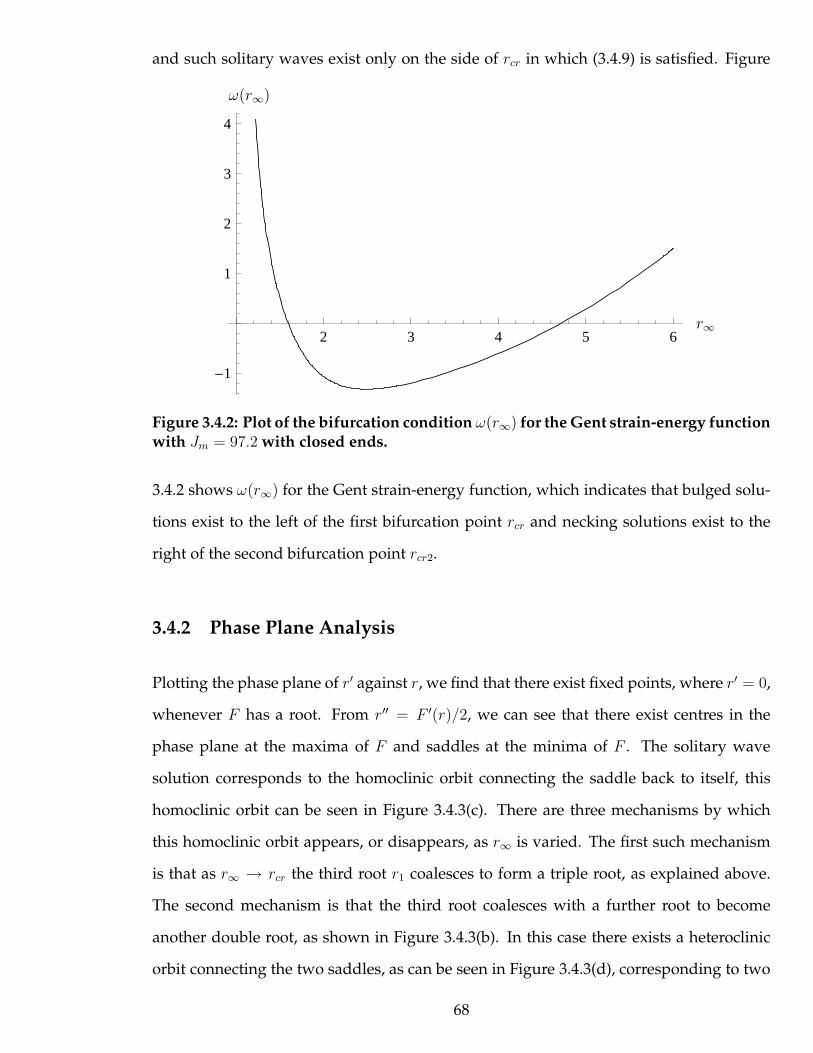
and such solitary waves exist only on the side of rcr in which (3.4.9) is satisfied. Figure

2 3 4 5 6

-1

1

2

3

4

r∞

ω(r∞)

Figure 3.4.2: Plot of the bifurcation condition ω(r∞) for the Gent strain-energy functionwith Jm = 97.2 with closed ends.

3.4.2 shows ω(r∞) for the Gent strain-energy function, which indicates that bulged solu-

tions exist to the left of the first bifurcation point rcr and necking solutions exist to the

right of the second bifurcation point rcr2.

3.4.2 Phase Plane Analysis

Plotting the phase plane of r′ against r, we find that there exist fixed points, where r′ = 0,

whenever F has a root. From r′′ = F ′(r)/2, we can see that there exist centres in the

phase plane at the maxima of F and saddles at the minima of F . The solitary wave

solution corresponds to the homoclinic orbit connecting the saddle back to itself, this

homoclinic orbit can be seen in Figure 3.4.3(c). There are three mechanisms by which

this homoclinic orbit appears, or disappears, as r∞ is varied. The first such mechanism

is that as r∞ → rcr the third root r1 coalesces to form a triple root, as explained above.

The second mechanism is that the third root coalesces with a further root to become

another double root, as shown in Figure 3.4.3(b). In this case there exists a heteroclinic

orbit connecting the two saddles, as can be seen in Figure 3.4.3(d), corresponding to two

68

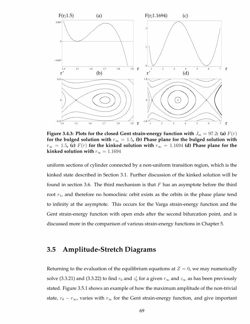
1.4 1.5 1.6 1.7 1.8 1.9

-0.007

0

0.007

1 2 3 4 5 6 70

1

2

1.4 1.5 1.6 1.7 1.8 1.9-0.15

0

0.15

1 2 3 4 5 6 7-1.8

0

1.8

rr

rr

(a) (c)

(b) (d)

F(r;1.5) F(r;1.1694)

r’ r’

Figure 3.4.3: Plots for the closed Gent strain-energy function with Jm = 97.2: (a) F (r)for the bulged solution with r∞ = 1.5, (b) Phase plane for the bulged solution withr∞ = 1.5, (c) F (r) for the kinked solution with r∞ = 1.1694 (d) Phase plane for thekinked solution with r∞ = 1.1694

uniform sections of cylinder connected by a non-uniform transition region, which is the

kinked state described in Section 3.1. Further discussion of the kinked solution will be

found in section 3.6. The third mechanism is that F has an asymptote before the third

root r1, and therefore no homoclinic orbit exists as the orbits in the phase plane tend

to infinity at the asymptote. This occurs for the Varga strain-energy function and the

Gent strain-energy function with open ends after the second bifurcation point, and is

discussed more in the comparison of various strain-energy functions in Chapter 5.

3.5 Amplitude-Stretch Diagrams

Returning to the evaluation of the equilibrium equations at Z = 0, we may numerically

solve (3.3.21) and (3.3.22) to find r0 and z′0 for a given r∞ and z∞ as has been previously

stated. Figure 3.5.1 shows an example of how the maximum amplitude of the non-trivial

state, r0 − r∞, varies with r∞ for the Gent strain-energy function, and give important

69

1 2 3 4 5 6

-4

-2

0

2

4

6

A

B

DF r∞

r0 − r∞(a)

1 2 3 4 5 6

1

2

3

4

5

6A

BC

D

E

F

G

r∞

r0(b)

Figure 3.5.1: Dependence of r0 − r∞ on r∞ for the closed Gent tube, Jm = 97.2. Onlythe solid lines in (a) correspond to localised solutions, and the non-localised solutionsare not plotted in (b)

insights to the bifurcation process. This plot corresponds to the non-trivial solution of

(3.3.21) and (3.3.22), combined with (3.3.18), and shows the amplitude of the bulging

or necking solutions. The existence of the solutions on one side of each critical point is

guaranteed by the shape of F in Figure 3.4.3 and also the shape of ω(r∞) in Figure 3.4.2.

The solid lines in Figure 3.5.1(a) correspond to where localised solutions do exist, given

by where the phase planes discussed in Section 3.4.2 have homoclinic orbits and are

verified numerically by the method detailed later in Section 3.7. Dashed lines represent

values of r0 and z′0 which satisfy (3.3.21) and (3.3.22) but do not satisfy the conditions

imposed in (3.3.16) specifying localised solutions. The localised solutions can cease to

exist through the methods discussed in Section 3.4.2 where the homoclinic orbit no longer

exists, and are not limited to turning points of the r0 − r∞ curve, although in this case

that is where the localised solutions disappear.

Figure 3.5.1(a) shows that, for the closed Gent strain-energy function with Jm = 97.2,

there exist two bifurcation points, the first of which corresponds to a bulged solution

and the second to a necking solution, as verified by the plot of ω(r∞) given in Figure

3.4.2. There also exist two points, marked A and B, where the gradient of r0 − r∞ be-

comes infinite. These two points, which will be denoted rk, are shown in section 3.6 to

70

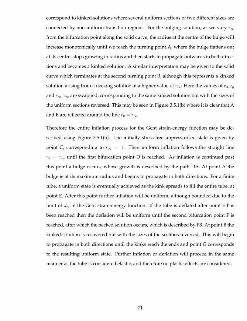
correspond to kinked solutions where several uniform sections of two different sizes are

connected by non-uniform transition regions. For the bulging solution, as we vary r∞

from the bifurcation point along the solid curve, the radius at the centre of the bulge will

increase monotonically until we reach the turning point A, where the bulge flattens out

at its centre, stops growing in radius and then starts to propagate outwards in both direc-

tions and becomes a kinked solution. A similar interpretation may be given to the solid

curve which terminates at the second turning point B, although this represents a kinked

solution arising from a necking solution at a higher value of r∞. Here the values of r0, z′0

and r∞, z∞ are swapped, corresponding to the same kinked solution but with the sizes of

the uniform sections reversed. This may be seen in Figure 3.5.1(b) where it is clear that A

and B are reflected around the line r0 = r∞.

Therefore the entire inflation process for the Gent strain-energy function may be de-

scribed using Figure 3.5.1(b). The initially stress-free unpressurised state is given by

point C, corresponding to r∞ = 1. Then uniform inflation follows the straight line

r0 = r∞ until the first bifurcation point D is reached. As inflation is continued past

this point a bulge occurs, whose growth is described by the path DA. At point A the

bulge is at its maximum radius and begins to propagate in both directions. For a finite

tube, a uniform state is eventually achieved as the kink spreads to fill the entire tube, at

point E. After this point further inflation will be uniform, although bounded due to the

limit of Jm in the Gent strain-energy function. If the tube is deflated after point E has

been reached then the deflation will be uniform until the second bifurcation point F is

reached, after which the necked solution occurs, which is described by FB. At point B the

kinked solution is recovered but with the sizes of the sections reversed. This will begin

to propagate in both directions until the kinks reach the ends and point G corresponds

to the resulting uniform state. Further inflation or deflation will proceed in the same

manner as the tube is considered elastic, and therefore no plastic effects are considered.

71

3.6 Kinked Solution

The location of a kinked solution where several uniform sections of differing sizes exist

may be found analytically, if such a value of r∞ exists. For a uniform state to exist at

Z = 0 we require, in addition to r′(0) = 0 as prescribed already, r′′(0) = 0. Subject to this

requirement, the equilibrium equation (3.3.7) becomes, using (3.3.5) and (3.3.16),

r0z′0W1(r∞, z∞) = r∞z∞W1(r0, z

′0). (3.6.1)

Therefore, combining (3.6.1) with (3.3.21), (3.3.22) and either the closed end condition

(3.3.18) or a specified z∞, we have a set of four equations for four unknowns, r0, z′0, r∞, z∞.

If a solution to these equations exists where r0 6= r∞, then this is the kinked solution, with

radius r0 at the origin and r∞ at infinity.

To show that the points where kinked solutions exist correspond to those marked A and

B in Figure 3.5.1, we first differentiate (3.3.21) and (3.3.22) with respect to r∞, viewing z′0

as a function of r∞ and r0, and r0, z∞ as functions of r∞, giving respectively,

∂r0∂r∞

(W12 − P ∗r0) +∂z′0∂r∞

W22 + P ∗r∞ +∂P ∗

∂r∞−W

(∞)12 − ∂z∞

∂r∞W

(∞)22 = 0 (3.6.2)

∂r0∂r∞

(W1 − z′0W12) +∂z′0∂r∞

z′0W22 −W(∞)1 + z∞W

(∞)12 +

∂z∞∂r∞

z∞W(∞)22 = 0. (3.6.3)

By taking the limit ∂r0/∂r∞ → ∞ in the resulting equations, corresponding to the tan-

gency observed in Figure 3.5.1, we obtain, using the chain rule on ∂z′0/∂r∞,

W12(r0, z′0) −

r0W(∞)1

r∞z∞+∂z′0∂r0

W22(r0, z′0) = 0, (3.6.4)

W1(r0, z′0) − z′0W12(r0, z

′0) + z′0

∂z′0∂r0

W22(r0, z′0) = 0, (3.6.5)

On eliminating ∂z′0/∂r0 between the two equations above, we reproduce the same condi-

tion as given by (3.6.1) by assuming r′′(0) = 0,

W1(r0, z′0) −

r0z′0

r∞z∞W

(∞)1 = 0. (3.6.6)

72

Therefore, at values of r∞ which satisfy (3.6.1), there exist two possible constant values

of r(Z) which satisfy the equilibrium equations; r∞ and r0. Therefore any combination

of uniform sections of radius r∞ and r0 connected by non-uniform transition regions is a

solution of the equilibrium equations.

We now proceed to show that these two uniform states satisfy the Maxwell equal-area

rule which occurs in other related kink-band problems (Ericksen 1975, Chater and Hutchin-

son 1984).

The Maxwell equal-area rule is that value of the pressure Pk such that the two areas

bounded by the pressure function P (v) and the line P = Pk are equal giving,

∫ v2

v1

P (v)dv = Pk(v2 − v1), (3.6.7)

where v is the volume of the tube. In the deformation considered here, the volume mea-

sure v is given by,

v = r2∞z∞, (3.6.8)

which for uniform inflation is the volume change per unit volume in the undeformed

configuration. With the additional use of (3.3.18) if required, we may view r∞ and z∞

both as functions of v. The two values of v generated by (3.6.7) are the volumes corre-

sponding to the two uniform sections of the kinked solution.

Figure 3.6.1 shows the pressure-volume curve for a typical closed Gent strain-energy

function, along with the line Pk which satisfies the equal-area rule. This pressure-volume

curve is typical for rubber-like materials, as discussed in Carroll (1987) and (Gent 2005),

but the pressure-volume curve is not required to be non-monotonic for the kinked solu-

tion to exist, as discussed below.

We now demonstrate that the equal-area condition (3.6.7) gives the same condition for the

kinked solutions as (3.6.1). We define the strain-energy depending solely on the volume

73

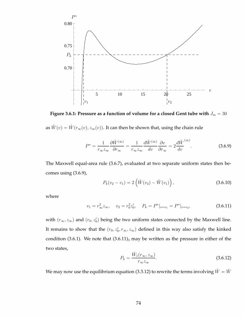
5 10 15 20 25

0.70

0.75

0.80

v

P ∗

v1 v2

Pk

Figure 3.6.1: Pressure as a function of volume for a closed Gent tube with Jm = 30

as W (v) = W (r∞(v), z∞(v)). It can then be shown that, using the chain rule

P ∗ =1

r∞z∞

∂W (∞)

∂r∞=

1

r∞z∞

dW (∞)

dv

∂v

∂r∞= 2

dW

dv

(∞)

. (3.6.9)

The Maxwell equal-area rule (3.6.7), evaluated at two separate uniform states then be-

comes using (3.6.9),

Pk(v2 − v1) = 2(

W (v2) − W (v1))

, (3.6.10)

where

v1 = r2∞z∞, v2 = r2

0z′0, Pk = P ∗|v=v1 = P ∗|v=v2 , (3.6.11)

with (r∞, z∞) and (r0, z′0) being the two uniform states connected by the Maxwell line.

It remains to show that the (r0, z′0, r∞, z∞) defined in this way also satisfy the kinked

condition (3.6.1). We note that (3.6.11)3 may be written as the pressure in either of the

two states,

Pk =W1(r∞, z∞)

r∞z∞. (3.6.12)

We may now use the equilibrium equation (3.3.12) to rewrite the terms involving W = W

74

on the right hand side of (3.6.10) in terms of W2 and C2, which along with (3.6.12) gives,

W1(r∞, z∞)

r∞z∞(r2

0z′0 − r2

∞z∞) = 2 (z′0W2(r0, z′0) − z∞W2(r∞, z∞)) . (3.6.13)

We can then use the other equilibrium equation (3.3.11) to express W2 in terms of W1 and

C1, which then reduces (3.6.13) to the kinked equation (3.6.1).

For the case of the Gent strain-energy function with z∞ = 1, P is a monotonic function

of v and thus no Maxwell line exists. However, the condition given by (3.6.6) still has a

solution which corresponds to the kinked solution, for example when Jm = 97.2, r∞ =

1.17643, r0 = 5.81723, z′0 = 4.09994 is a solution to (3.6.6). In this case, the two pressures

given by (3.6.11)3 evaluated at the two pairs (r∞, 1) and (r0, z′0) are equal, and therefore

we conclude that the condition (3.6.1) is the requirement for the kink to exist, not the

existence of the Maxwell line.

3.7 Numerical Solutions

We now look at directly solving the equilibrium equations given in (3.3.11) and (3.3.12)

numerically, subject to the localised behaviour specified in (3.3.15). In doing so we can

find, for the regions where it exists, the solitary wave solution or the kinked solution for a

given r∞, z∞ and strain-energy function. Initially we may take the first order differential

equation derived in (3.4.4) and rewrite it as,

∫ r0

r(Z)

dr

∓√

F (r; r∞)=

∫ 0

Z

dZ, (3.7.1)

where we take the negative sign for regions of bulging solutions as r′(Z) < 0, and the

positive sign for necking solutions. Evaluating (3.7.1) at successive values of Z is a very

accurate but computationally expensive method of finding the bifurcated solution for

r(Z), which then can be used to find z(Z).

75

Kyriakides and Chang (1991) give a set of differential equations which may be used to

find r(Z) and z(Z), without using the conservation laws (3.3.11) and (3.3.12). This is an

equivalent set of differential equations to (3.3.6) and (3.3.7), but using λ1, λ2 and φ as the

independent coordinates, where φ is the angle between the Z-axis and the membrane,

defined in Figure 3.3.1:

λ′1 = λ2 sinφ,

λ′2 =W1 − λ2W12

W22

sinφ, (3.7.2)

θ′ =W1

W2

cosφ− W(∞)1

r∞z∞W2

λ1λ2.

Equations (3.7.2) are solved subject to the initial conditions λ1(0) = r0, λ2(0) = z′0, φ(0) =

0, the last of these coming from the fact that the deformed tube is flat at Z = 0 as we

impose r′(0) = 0 in the symmetry conditions. Using (3.7.2) is computationally more

efficient than using (3.7.1) for solving the equilibrium equation and gives the same re-

sults. Consequently, it was the numerical scheme used throughout the work presented

here, although comparison with the integral (3.7.1) was made for selected cases to ensure

the results are accurate. Back substitution of the computed results into the equilibrium

equations was also used to verify the accuracy of the solutions.

Figure 3.7.1 shows typical profiles of r(Z) for the solitary wave solution with varying r∞

for the Gent strain-energy function with Jm = 97.2. This shows how the bulge increases

while the far-radius decreases, as expected from the amplitude-stretch diagram given in

Figure 3.5.1. In addition, it shows how the solution stops growing radially, flattens and

propagates down the tube as the kinked solution is approached. However, in Figure

3.7.1 the radius is plotted against the position in the undeformed axial variable Z. In

order to visualise the tube in the deformed configuration it is necessary to plot r(Z)

against z(Z), as shown in Figure 3.7.2, compared to the undeformed configuration where

−10 < Z < 10. This second plot shows how the axial stretch z′(Z) is involved in the

deformation, and it is greater than unity for the bulged configuration. Figure 3.7.3 shows

76

how the deformed tube expands and approaches the kinked solution as r∞ → rk.

-10 -5 5 10

1.4

1.6

1.8

2.0

2.2

2.4

2.6

Z

r(Z)

r∞ = 1.3

r∞ = 1.4

r∞ = 1.5

r∞ = 1.55

r∞ = 1.58

Figure 3.7.1: Profiles of r(Z) for a closed Gent tube with Jm = 97.2.

-10 -5 5 10

1.4

1.6

1.8

2.0

2.2

2.4

2.6

z(Z)

r(Z)

r∞ = 1.3

r∞ = 1.4

r∞ = 1.5

r∞ = 1.55

r∞ = 1.58

Figure 3.7.2: Deformed configurations for a closed Gent tube with Jm = 97.2.

3.8 Conclusion

This chapter has detailed the conditions required for bulging or necking solutions to

exist, and shown how the amplitude-stretch diagram discussed in (3.5) imparts a great

amount of information about the process. The bifurcation condition, ω(r∞) = 0, may

be calculated easily for any given strain-energy function by using (3.4.5) and the side

77

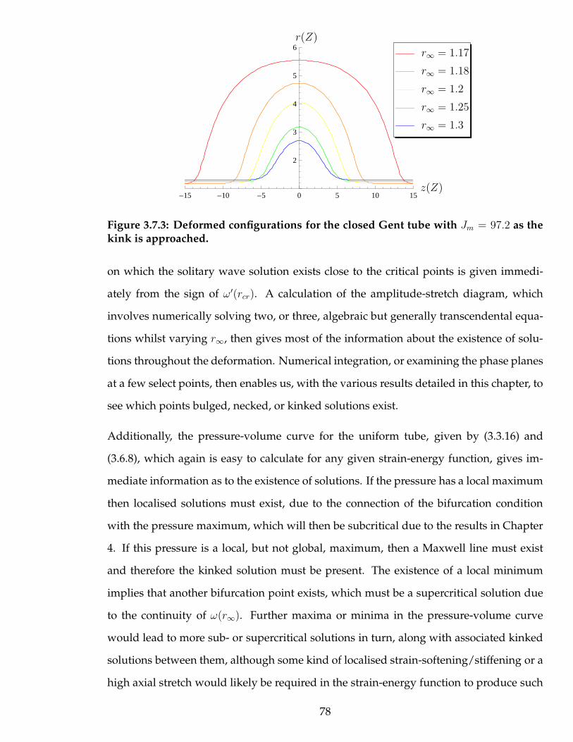
-15 -10 -5 0 5 10 15

2

3

4

5

6

z(Z)

r(Z)

r∞ = 1.17

r∞ = 1.18

r∞ = 1.2

r∞ = 1.25

r∞ = 1.3

Figure 3.7.3: Deformed configurations for the closed Gent tube with Jm = 97.2 as thekink is approached.

on which the solitary wave solution exists close to the critical points is given immedi-

ately from the sign of ω′(rcr). A calculation of the amplitude-stretch diagram, which

involves numerically solving two, or three, algebraic but generally transcendental equa-

tions whilst varying r∞, then gives most of the information about the existence of solu-

tions throughout the deformation. Numerical integration, or examining the phase planes

at a few select points, then enables us, with the various results detailed in this chapter, to

see which points bulged, necked, or kinked solutions exist.

Additionally, the pressure-volume curve for the uniform tube, given by (3.3.16) and

(3.6.8), which again is easy to calculate for any given strain-energy function, gives im-

mediate information as to the existence of solutions. If the pressure has a local maximum

then localised solutions must exist, due to the connection of the bifurcation condition

with the pressure maximum, which will then be subcritical due to the results in Chapter

4. If this pressure is a local, but not global, maximum, then a Maxwell line must exist

and therefore the kinked solution must be present. The existence of a local minimum

implies that another bifurcation point exists, which must be a supercritical solution due

to the continuity of ω(r∞). Further maxima or minima in the pressure-volume curve

would lead to more sub- or supercritical solutions in turn, along with associated kinked

solutions between them, although some kind of localised strain-softening/stiffening or a

high axial stretch would likely be required in the strain-energy function to produce such

78

a pressure-volume relationship.

It is not currently clear why the Maxwell line is not required for a kinked solution to

exist, as in the Gent tube where the pressure-volume curve for the uniform tube is mono-

tonically increasing. This requires further investigation, particularly in the case of open-

ended tubes.

79

Chapter 4

Stability of a Bifurcated Cylindrical

Membrane

4.1 Introduction

Chapter 3 showed the existence of bifurcated states of the cylindrical tube, and this chap-

ter considers the stability of these bifurcated states with respect to axisymmetric pertur-

bations. Initially, we discuss the stability of the uniformly inflated tube which is shown to

be initially stable at r∞ = 1 and change stability at the bifurcation points rcr. We derive

the dispersion relation for the inflated tube and use this to construct a suitable pertur-

bation expansion in order to derive an evolution equation which the weakly nonlinear

equation is related to. Inserting into this evolution equation a time-dependent perturba-

tion we find an eigenvalue problem, which we solve using the Evans function as part of

the compound matrix method. In this way we show that the weakly nonlinear solution

is always unstable, for both bulging or necking cases and any strain-energy function.

After this we proceed by considering the spectral stability of the fully nonlinear bulged

or necked solution using the same method, and show numerically that it is unstable.

An alternative stability test using an energy method is used to investigate the bifurcated

80

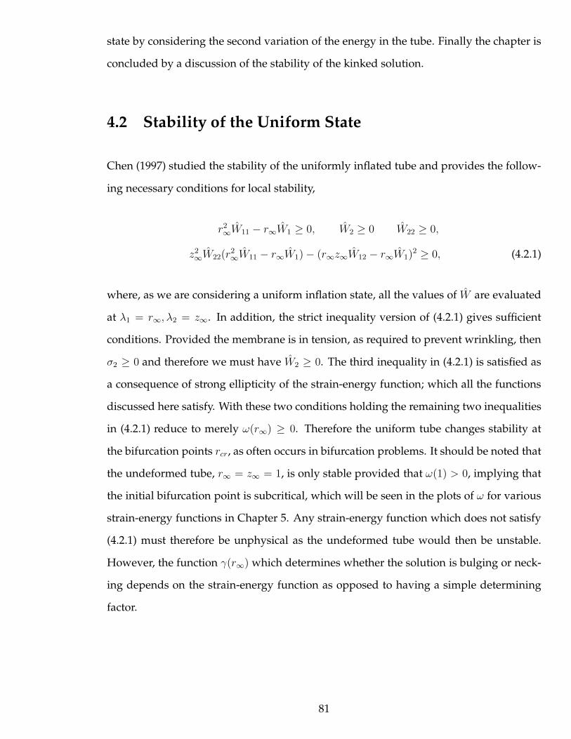
state by considering the second variation of the energy in the tube. Finally the chapter is

concluded by a discussion of the stability of the kinked solution.

4.2 Stability of the Uniform State

Chen (1997) studied the stability of the uniformly inflated tube and provides the follow-

ing necessary conditions for local stability,

r2∞W11 − r∞W1 ≥ 0, W2 ≥ 0 W22 ≥ 0,

z2∞W22(r

2∞W11 − r∞W1) − (r∞z∞W12 − r∞W1)

2 ≥ 0, (4.2.1)

where, as we are considering a uniform inflation state, all the values of W are evaluated

at λ1 = r∞, λ2 = z∞. In addition, the strict inequality version of (4.2.1) gives sufficient

conditions. Provided the membrane is in tension, as required to prevent wrinkling, then

σ2 ≥ 0 and therefore we must have W2 ≥ 0. The third inequality in (4.2.1) is satisfied as

a consequence of strong ellipticity of the strain-energy function; which all the functions

discussed here satisfy. With these two conditions holding the remaining two inequalities

in (4.2.1) reduce to merely ω(r∞) ≥ 0. Therefore the uniform tube changes stability at

the bifurcation points rcr, as often occurs in bifurcation problems. It should be noted that

the undeformed tube, r∞ = z∞ = 1, is only stable provided that ω(1) > 0, implying that

the initial bifurcation point is subcritical, which will be seen in the plots of ω for various

strain-energy functions in Chapter 5. Any strain-energy function which does not satisfy

(4.2.1) must therefore be unphysical as the undeformed tube would then be unstable.

However, the function γ(r∞) which determines whether the solution is bulging or neck-

ing depends on the strain-energy function as opposed to having a simple determining

factor.

81

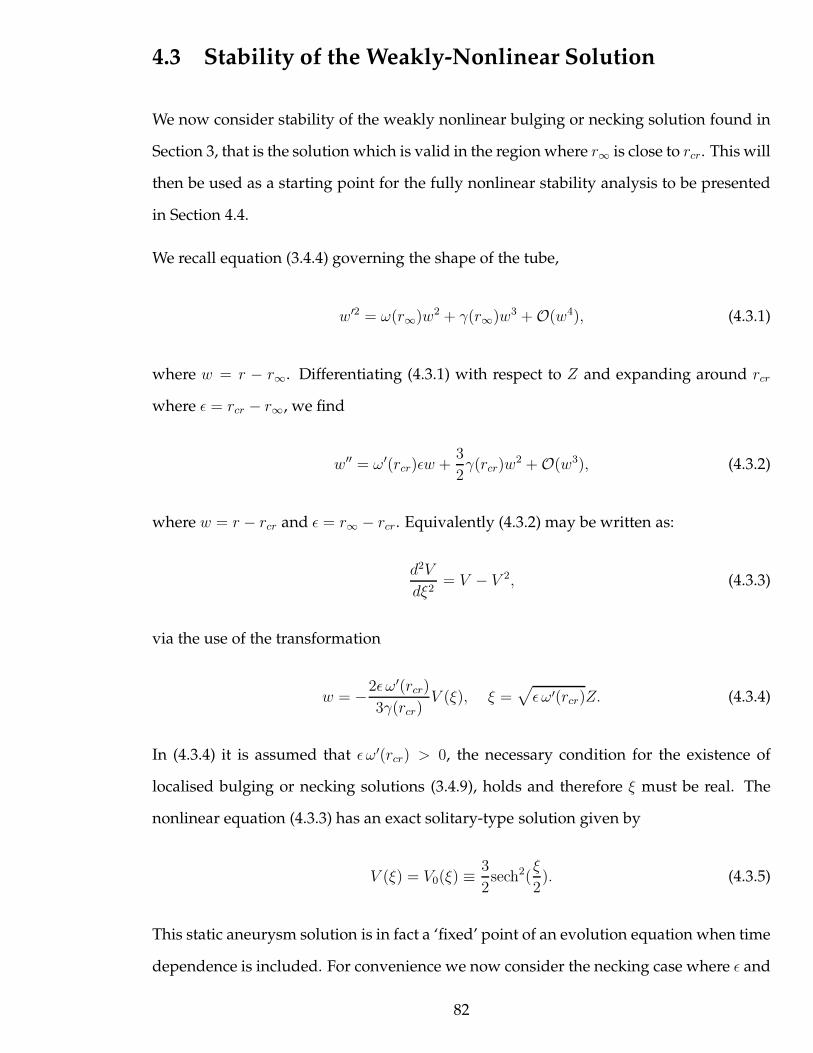
4.3 Stability of the Weakly-Nonlinear Solution

We now consider stability of the weakly nonlinear bulging or necking solution found in

Section 3, that is the solution which is valid in the region where r∞ is close to rcr. This will

then be used as a starting point for the fully nonlinear stability analysis to be presented

in Section 4.4.

We recall equation (3.4.4) governing the shape of the tube,

w′2 = ω(r∞)w2 + γ(r∞)w3 + O(w4), (4.3.1)

where w = r − r∞. Differentiating (4.3.1) with respect to Z and expanding around rcr

where ǫ = rcr − r∞, we find

w′′ = ω′(rcr)ǫw +3

2γ(rcr)w

2 + O(w3), (4.3.2)

where w = r − rcr and ǫ = r∞ − rcr. Equivalently (4.3.2) may be written as:

d2V

dξ2= V − V 2, (4.3.3)

via the use of the transformation

w = −2ǫ ω′(rcr)

3γ(rcr)V (ξ), ξ =

√

ǫ ω′(rcr)Z. (4.3.4)

In (4.3.4) it is assumed that ǫ ω′(rcr) > 0, the necessary condition for the existence of

localised bulging or necking solutions (3.4.9), holds and therefore ξ must be real. The

nonlinear equation (4.3.3) has an exact solitary-type solution given by

V (ξ) = V0(ξ) ≡3

2sech2(

ξ

2). (4.3.5)

This static aneurysm solution is in fact a ‘fixed’ point of an evolution equation when time

dependence is included. For convenience we now consider the necking case where ǫ and

82

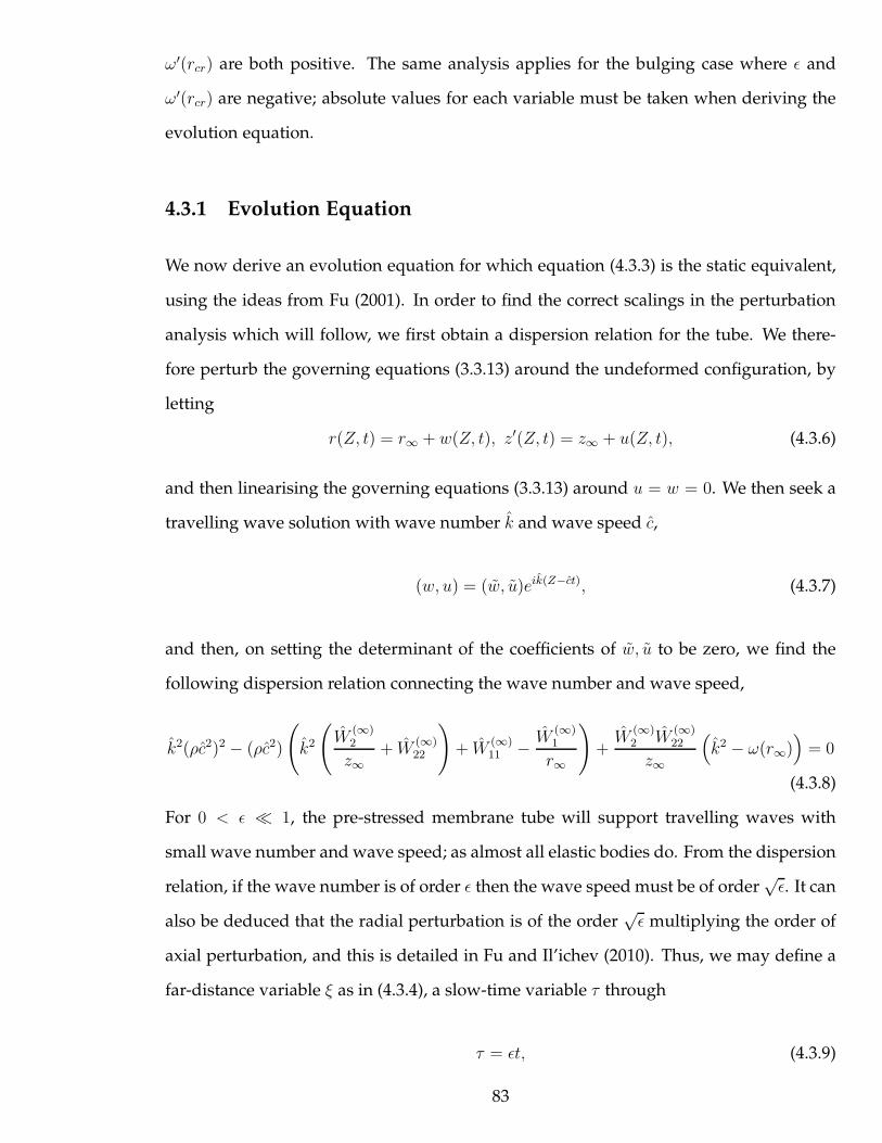
ω′(rcr) are both positive. The same analysis applies for the bulging case where ǫ and

ω′(rcr) are negative; absolute values for each variable must be taken when deriving the

evolution equation.

4.3.1 Evolution Equation

We now derive an evolution equation for which equation (4.3.3) is the static equivalent,

using the ideas from Fu (2001). In order to find the correct scalings in the perturbation

analysis which will follow, we first obtain a dispersion relation for the tube. We there-

fore perturb the governing equations (3.3.13) around the undeformed configuration, by

letting

r(Z, t) = r∞ + w(Z, t), z′(Z, t) = z∞ + u(Z, t), (4.3.6)

and then linearising the governing equations (3.3.13) around u = w = 0. We then seek a

travelling wave solution with wave number k and wave speed c,

(w, u) = (w, u)eik(Z−ct), (4.3.7)

and then, on setting the determinant of the coefficients of w, u to be zero, we find the

following dispersion relation connecting the wave number and wave speed,

k2(ρc2)2 − (ρc2)

(

k2

(

W(∞)2

z∞+ W

(∞)22

)

+ W(∞)11 − W

(∞)1

r∞

)

+W

(∞)2 W

(∞)22

z∞

(

k2 − ω(r∞))

= 0

(4.3.8)

For 0 < ǫ ≪ 1, the pre-stressed membrane tube will support travelling waves with

small wave number and wave speed; as almost all elastic bodies do. From the dispersion

relation, if the wave number is of order ǫ then the wave speed must be of order√ǫ. It can

also be deduced that the radial perturbation is of the order√ǫ multiplying the order of

axial perturbation, and this is detailed in Fu and Il’ichev (2010). Thus, we may define a

far-distance variable ξ as in (4.3.4), a slow-time variable τ through

τ = ǫt, (4.3.9)

83

and look for a perturbation solution of the form

r = rcr + ǫλ1 + ǫ {w1(ξ, τ) + ǫw2(ξ, τ) + · · · } , (4.3.10)

z = (zcr + ǫλ2)Z +√ǫ {u1(ξ, τ) + ǫu2(ξ, τ) + · · · } , (4.3.11)

where w1, w2, u1, u2, λ1, λ2 are all order one functions and zcr = z∞(rcr) is the critical value

of z∞. We also note that the internal pressure is given by (3.3.16), so that when r∞ and

z∞ are perturbed as ǫ = r∞ − rcr, P ∗ expands as

P ∗ = P0 + ǫP1 + · · · , (4.3.12)

where again P0 and P1 are order one functions. We now substitute (4.3.10), (4.3.11) and

(4.3.12) into the equations of motion, (3.3.13), and equate the powers of ǫ. We find at first

order in ǫ, after integrating one equation, two equations for w1(ξ) and u1ξ(ξ), which may

be rewritten as,

L

w1

√

ω′(rcr)u1ξ

= 0, where L =

−W1/zcr + W12 W22

zcr(W1 − rcrW11) rcr(W1 − zcrW12)

,

(4.3.13)

where W1, W2, W12, W22 are all evaluated at r = rcr, z′ = zcr, and u1ξ denotes ∂u1/∂ξ.

Clearly, detL = ω(rcr)rcrW2W22. Thus, as we expected, ω(rcr) = 0 ensures that the matrix

equation (4.3.13) has a non-trivial solution for w1 and u1. Proceeding to the next order,

we find that w2 and u2 satisfy the inhomogeneous system

L

w2

√

ω′(rcr)u2ξ

= b, (4.3.14)

where the vector b only contains w1 and its derivatives. As the matrix L is singular as

discussed above, we now need to impose a solvability condition in order to be able to

find a solution to (4.3.14). We do this by taking the dot product of (4.3.14) with the left

eigenvector of L, resulting in a zero left hand side of the resulting equation from the

84

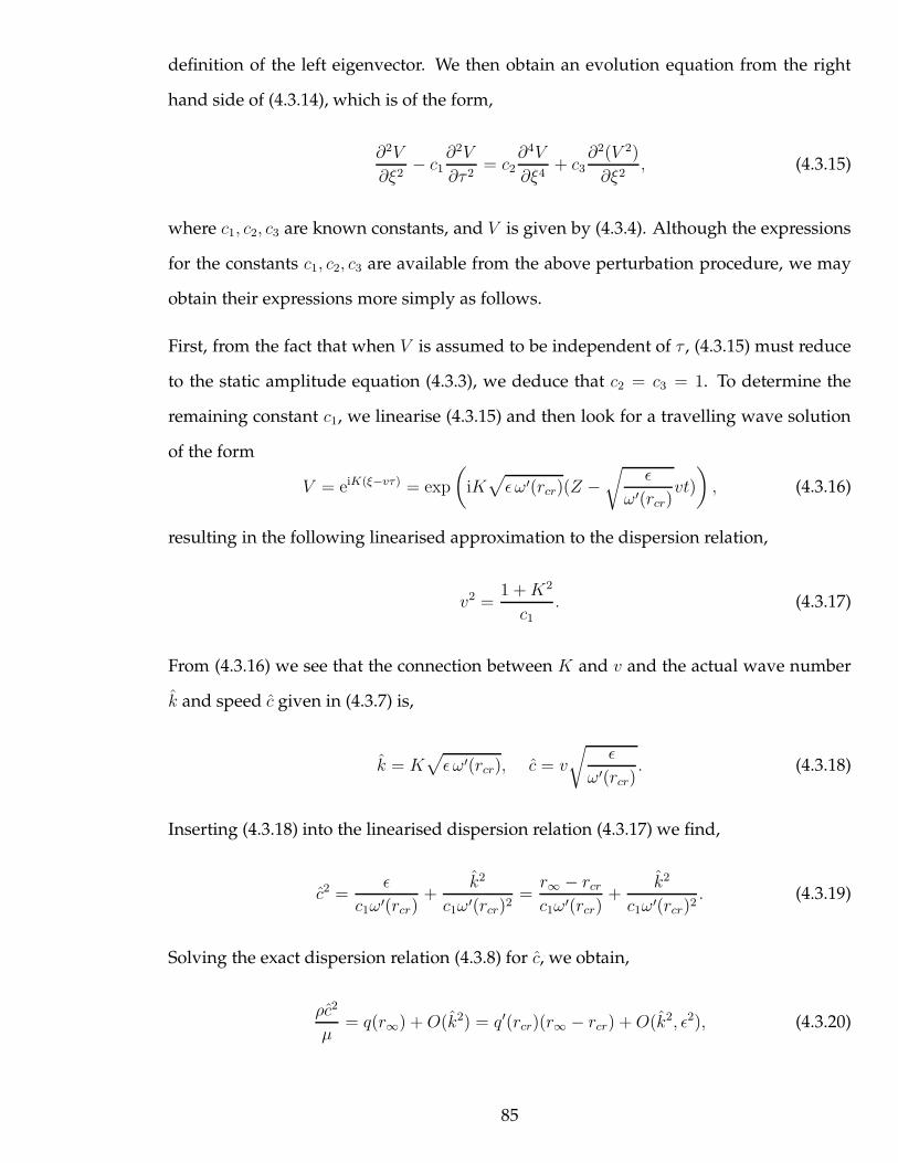
definition of the left eigenvector. We then obtain an evolution equation from the right

hand side of (4.3.14), which is of the form,

∂2V

∂ξ2− c1

∂2V

∂τ 2= c2

∂4V

∂ξ4+ c3

∂2(V 2)

∂ξ2, (4.3.15)

where c1, c2, c3 are known constants, and V is given by (4.3.4). Although the expressions

for the constants c1, c2, c3 are available from the above perturbation procedure, we may

obtain their expressions more simply as follows.

First, from the fact that when V is assumed to be independent of τ , (4.3.15) must reduce

to the static amplitude equation (4.3.3), we deduce that c2 = c3 = 1. To determine the

remaining constant c1, we linearise (4.3.15) and then look for a travelling wave solution

of the form

V = eiK(ξ−vτ) = exp

(

iK√

ǫ ω′(rcr)(Z −√

ǫ

ω′(rcr)vt)

)

, (4.3.16)

resulting in the following linearised approximation to the dispersion relation,

v2 =1 +K2

c1. (4.3.17)

From (4.3.16) we see that the connection between K and v and the actual wave number

k and speed c given in (4.3.7) is,

k = K√

ǫ ω′(rcr), c = v

√ǫ

ω′(rcr). (4.3.18)

Inserting (4.3.18) into the linearised dispersion relation (4.3.17) we find,

c2 =ǫ

c1ω′(rcr)+

k2

c1ω′(rcr)2=r∞ − rcr

c1ω′(rcr)+

k2

c1ω′(rcr)2. (4.3.19)

Solving the exact dispersion relation (4.3.8) for c, we obtain,

ρc2

µ= q(r∞) +O(k2) = q′(rcr)(r∞ − rcr) +O(k2, ǫ2), (4.3.20)

85

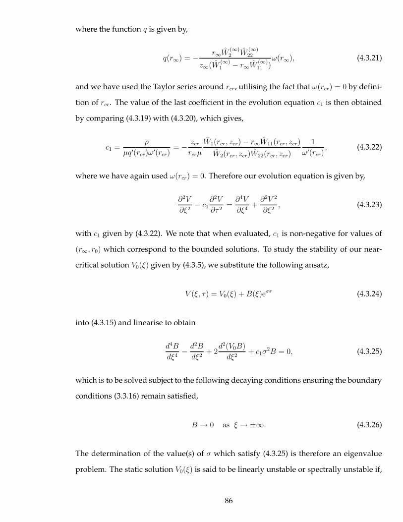
where the function q is given by,

q(r∞) = − r∞W(∞)2 W

(∞)22

z∞(W(∞)1 − r∞W

(∞)11 )

ω(r∞), (4.3.21)

and we have used the Taylor series around rcr, utilising the fact that ω(rcr) = 0 by defini-

tion of rcr. The value of the last coefficient in the evolution equation c1 is then obtained

by comparing (4.3.19) with (4.3.20), which gives,

c1 =ρ

µq′(rcr)ω′(rcr)= − zcr

rcrµ

W1(rcr, zcr) − r∞W11(rcr, zcr)

W2(rcr, zcr)W22(rcr, zcr)

1

ω′(rcr), (4.3.22)

where we have again used ω(rcr) = 0. Therefore our evolution equation is given by,

∂2V

∂ξ2− c1

∂2V

∂τ 2=∂4V

∂ξ4+∂2V 2

∂ξ2, (4.3.23)

with c1 given by (4.3.22). We note that when evaluated, c1 is non-negative for values of

(r∞, r0) which correspond to the bounded solutions. To study the stability of our near-

critical solution V0(ξ) given by (4.3.5), we substitute the following ansatz,

V (ξ, τ) = V0(ξ) +B(ξ)eστ (4.3.24)

into (4.3.15) and linearise to obtain

d4B

dξ4− d2B

dξ2+ 2

d2(V0B)

dξ2+ c1σ

2B = 0, (4.3.25)

which is to be solved subject to the following decaying conditions ensuring the boundary

conditions (3.3.16) remain satisfied,

B → 0 as ξ → ±∞. (4.3.26)

The determination of the value(s) of σ which satisfy (4.3.25) is therefore an eigenvalue

problem. The static solution V0(ξ) is said to be linearly unstable or spectrally unstable if,

86

for some fixed complex σ with Re (σ) > 0, there exists a solution of (4.3.25) which decays

exponentially as ξ → ±∞.

4.3.2 Compound Matrix Method

We therefore solve this eigenvalue problem by computing the Evans function for the

compound matrix method as discussed in Section 2.5. We follow the procedure explained

in Afendikov and Bridges (2001) in which the eigenvalue problem also involves a fourth-

order differential equation. We rewrite the system (4.3.25) as a matrix system of first

order differential equations as,

y′ = A(ξ)y, (4.3.27)

where y = (B(ξ), B′(ξ), B′′(ξ), B′′′(ξ))T , and the matrix A is given by,

A(ξ; ζ) =

0 1 0 0

0 0 1 0

0 0 0 1

−ζ − 2V ′′0 (ξ) −4V ′

0(ξ) 1 − 2V0(ξ) 0

, (4.3.28)

where ζ = c1σ2. Evaluating (4.3.28) at ξ → ∞, we find,

A∞ =

0 1 0 0

0 0 1 0

0 0 0 1

−ζ 0 1 0

, (4.3.29)

which has two pairs of eigenvalues, given by ±k1,±k2, where k1 =√

12(1 −

√1 − 4ζ),

k2 =√

12(1 +

√1 − 4ζ), which will be denoted as matrix eigenvalues to distinguish them

from the eigenvalues of the eigenproblem under consideration. Associated with each

of these matrix eigenvalues is an eigenvector, and we denote the two eigenvectors as-

sociated with k1, k2 as a−1 ,a

−2 respectively, and those associated with −k1,−k2 as a+

1 ,a+2

87

respectively. As ξ → ∞, any decaying solution of (4.3.27) will be a linear combination of

a+1 e−k1ξ and a+

2 e−k2ξ and the nomenclature becomes clear. Similarly, as ξ → −∞ decaying

solutions will be a linear combination of a−1 ek1ξ and a−

2 ek2ξ.

For a fixed ζ we may integrate from −L using a−1 with k1, resulting in a solution y−

1 (ξ),

where L is a large number used instead of infinity for the numerical results. Similarly,

we can find a second solution y−2 (ξ) from using a−

2 , and two solutions which come from

integrating from L, y+1 (ξ) and y+

2 (ξ). Naively, we could then attempt to find a value of ζ

such that the solutions intersect in a non-trivial way, namely that the determinant formed

by (y−1 (ξ)y−

2 (ξ)y+1 (ξ)y+

2 (ξ)) is zero at a specific ξ.

However, we use the compound matrix method as discussed in Section 2.5.3, which en-

sures that the differential equations are non-stiff. The disadvantage of the compound

matrix method is that it converts a system of order 2n into a system of order n(n+1) and

is hence impractical for large n, but this is an acceptable compromise here where n = 2

and therefore we change from fourth order to sixth order.

We define two new matrices M−(ξ) and M+(ξ) by concatenating the two appropriate

solutions, as discussed in Section 2.5.3, along with the two sets of minors φ−i and φ+

i . We

therefore reach a sixth order differential system, where (4.3.27) becomes

φ′ = Q(ξ)φ, (4.3.30)

where Q is given by (2.5.14).

The two sets of initial conditions for the φi are given by the corresponding minors of

M−(−L) andM+(L), and then (4.3.30) is integrated from both sides for a given ζ . How-

ever, to remove the exponential growth which the solutions must obey in this case we

write φ(ξ) = ψ(ξ)eKξ, where K = k1 + k2 for integration from −L and K = −(k1 + k2) for

the integration from L, and therefore (4.3.30) becomes

ψ′ = (Q −KI)ψ, (4.3.31)

88

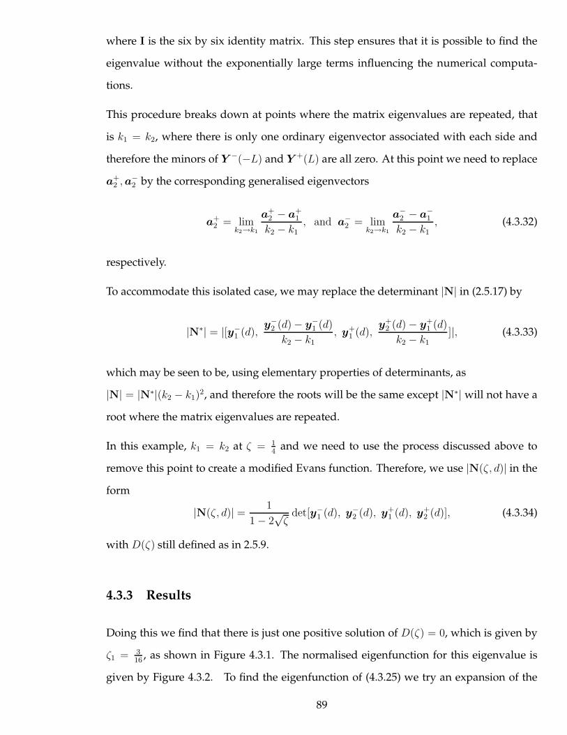
where I is the six by six identity matrix. This step ensures that it is possible to find the

eigenvalue without the exponentially large terms influencing the numerical computa-

tions.

This procedure breaks down at points where the matrix eigenvalues are repeated, that

is k1 = k2, where there is only one ordinary eigenvector associated with each side and

therefore the minors of Y −(−L) and Y +(L) are all zero. At this point we need to replace

a+2 ,a

−2 by the corresponding generalised eigenvectors

a+2 = lim

k2→k1

a+2 − a+

1

k2 − k1, and a−

2 = limk2→k1

a−2 − a−

1

k2 − k1, (4.3.32)

respectively.

To accommodate this isolated case, we may replace the determinant |N| in (2.5.17) by

|N∗| = |[y−1 (d),

y−2 (d) − y−

1 (d)

k2 − k1, y+

1 (d),y+

2 (d) − y+1 (d)

k2 − k1]|, (4.3.33)

which may be seen to be, using elementary properties of determinants, as

|N| = |N∗|(k2 − k1)2, and therefore the roots will be the same except |N∗| will not have a

root where the matrix eigenvalues are repeated.

In this example, k1 = k2 at ζ = 14

and we need to use the process discussed above to

remove this point to create a modified Evans function. Therefore, we use |N(ζ, d)| in the

form

|N(ζ, d)| = 1

1 − 2√ζ

det[y−1 (d), y−

2 (d), y+1 (d), y+

2 (d)], (4.3.34)

with D(ζ) still defined as in 2.5.9.

4.3.3 Results

Doing this we find that there is just one positive solution of D(ζ) = 0, which is given by

ζ1 = 316

, as shown in Figure 4.3.1. The normalised eigenfunction for this eigenvalue is

given by Figure 4.3.2. To find the eigenfunction of (4.3.25) we try an expansion of the

89

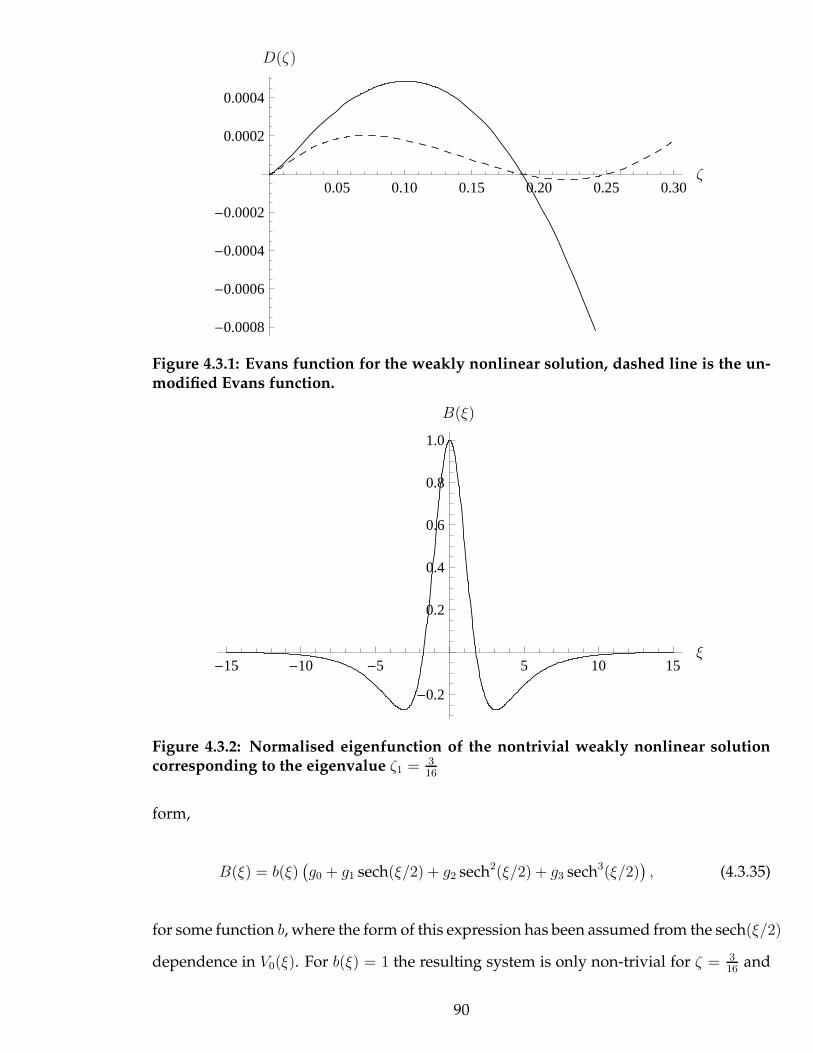
0.05 0.10 0.15 0.20 0.25 0.30

-0.0008

-0.0006

-0.0004

-0.0002

0.0002

0.0004

ζ

D(ζ)

Figure 4.3.1: Evans function for the weakly nonlinear solution, dashed line is the un-modified Evans function.

-15 -10 -5 5 10 15

-0.2

0.2

0.4

0.6

0.8

1.0

ξ

B(ξ)

Figure 4.3.2: Normalised eigenfunction of the nontrivial weakly nonlinear solutioncorresponding to the eigenvalue ζ1 = 3

16

form,

B(ξ) = b(ξ)(g0 + g1 sech(ξ/2) + g2 sech2(ξ/2) + g3 sech3(ξ/2)

), (4.3.35)

for some function b, where the form of this expression has been assumed from the sech(ξ/2)

dependence in V0(ξ). For b(ξ) = 1 the resulting system is only non-trivial for ζ = 316

and

90

may be simplified to

B(ξ) = B0

(

2 sech3

(ξ

2

)

− sech

(ξ

2

))

, (4.3.36)

where B0 is an arbitrary amplitude. Therefore the analytic expression for the eigenfunc-

tion corresponding to ζ1 is given by (4.3.36). For b(ξ) = tanh(ξ/2), the eigenvalue at zero

has an eigenfunction given by,

B(ξ) = B1V′0(ξ) = −3B1

4tanh

(ξ

2

)

sech

(ξ

2

)

, (4.3.37)

where B1 is an arbitrary amplitude. Therefore, as the above analysis is for a general

strain-energy function and either the bulging or necking near-critical solution, we state

that all such near-critical solutions are unstable with respect to axisymmetric perturba-

tions.

4.4 Stability of the General Bifurcated State

4.4.1 Introduction

In this section we consider the stability of the fully nonlinear bifurcated solution with

respect to spectral perturbations of the form a(Z)eηt, in the same way as in the section

4.3 for the weakly nonlinear solution. We insert these perturbations into the equations of

motion and linearise, resulting in a differential equation for the unknown function a(Z)

which depends on η. This equation will then be solved subject to the boundary condition

that a(Z) decays as Z → ∞.

91

4.4.2 Governing Equations

We therefore insert into the equations of motion (3.3.13) perturbations of the general

form,

r(Z, t) = r(Z) + w(Z, t), z(Z, t) = z(Z) + u(Z, t), (4.4.1)

where r and z are the static non-trivial solutions found from the integration of the in-

tegrated governing equations (3.3.11) and (3.3.12), as discussed in Chapter 3. Note that

r and z both depend on r∞, z∞ and the form of W . Inserting (4.4.1) into (3.3.13) and

linearising around the static state we find:

[W2u

′ + z′

λ22(λ2W22 − W2)(r

′w′ + z′u′) + wz′W12

λ2

]′

− P ∗(rw′ + wr′) = ρu, (4.4.2)

[W2w

′ + r′

λ22(λ2W22 − W2)(r

′w′ + z′u′) + r′r1W12

λ2

]′

− W12

λ2

(r′w′ + z′u′) − wW11 − P ∗(ru′ + wz′) = ρw, (4.4.3)

where λ2 =√r′2 + z′2 and a bar indicates evaluation at the known values of r = r, z = z.

It should be noted that P ∗ in (4.4.2) and (4.4.3) is also a function of r∞ as given by (3.3.16).

We then assume that the perturbations have an exponential time dependence given by,

w(Z, t) = w(Z)eηt, u(Z, t) = u(Z)eηt, (4.4.4)

introducing η as the eigenvalue. It is clear that if η has a positive real part then the am-

plitude of the perturbation will grow exponentially in time, and hence the static solution

is unstable.

It can be seen that (4.4.2) and (4.4.3), after use of (4.4.4), is a system of two coupled linear

second order ordinary differential equations in w(Z) and u(Z), and the dependence on

η is entirely through the combination α = ρη2, which defines α. The determination of

92

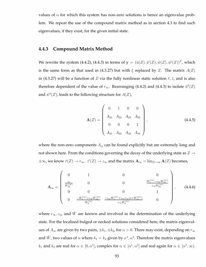
values of α for which this system has non-zero solutions is hence an eigenvalue prob-

lem. We repeat the use of the compound matrix method as in section 4.3 to find such

eigenvalues, if they exist, for the given initial state.

4.4.3 Compound Matrix Method

We rewrite the system (4.4.2), (4.4.3) in terms of y = (u(Z), u′(Z), w(Z), w′(Z))T , which

is the same form as that used in (4.3.27) but with ξ replaced by Z. The matrix A(Z)

in (4.3.27) will be a function of Z via the fully nonlinear static solution r, z, and is also

therefore dependent of the value of r∞. Rearranging (4.4.2) and (4.4.3) to isolate u′′(Z)

and w′′(Z), leads to the following structure for A(Z),

A(Z) =

0 1 0 0

A21 A22 A23 A24

0 0 0 1

A41 A42 A43 A44

, (4.4.5)

where the non-zero components Aij can be found explicitly but are extremely long and

not shown here. From the conditions governing the decay of the underlying state as Z →

±∞, we know r(Z) → r∞, z′(Z) → z∞ and the matrix A∞ = limZ→∞ A(Z) becomes,

A∞ =

0 1 0 0

α

W(∞)22

0 0W

(∞)1 −z∞W

(∞)12

z∞W(∞)22

0 0 0 1

0−W

(∞)1 +z∞W

(∞)12

W(∞)2

−z∞W(∞)1 +z∞r∞(α+W

(∞)11 )

r∞W(∞)2

0

, (4.4.6)

where r∞, z∞ and W are known and involved in the determination of the underlying

state. For the localised bulged or necked solutions considered here, the matrix eigenval-

ues of A∞ are given by two pairs, ±k1,±k2, for α > 0. There may exist, depending on r∞

and W , two values of α where k1 = k2 given by α1, α2. Therefore the matrix eigenvalues

k1 and k2 are real for α ∈ [0, α1], complex for α ∈ [α1, α2] and real again for α ∈ [α2,∞).

93

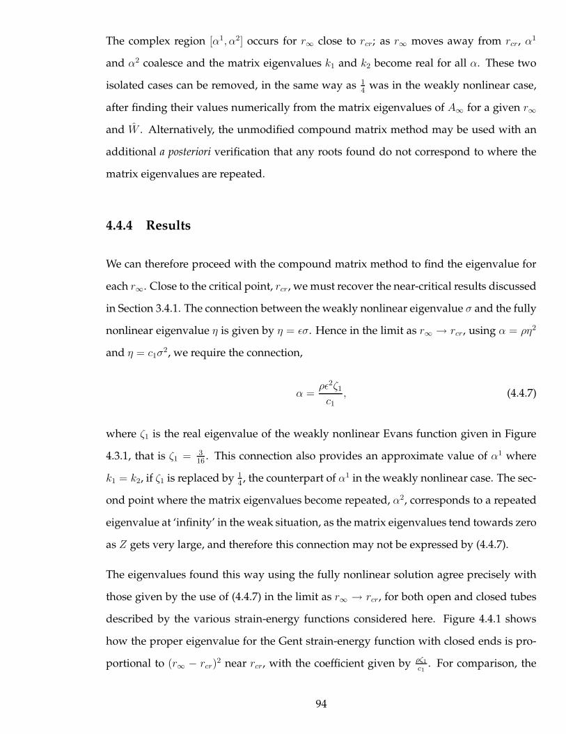
The complex region [α1, α2] occurs for r∞ close to rcr; as r∞ moves away from rcr, α1

and α2 coalesce and the matrix eigenvalues k1 and k2 become real for all α. These two

isolated cases can be removed, in the same way as 14

was in the weakly nonlinear case,

after finding their values numerically from the matrix eigenvalues of A∞ for a given r∞

and W . Alternatively, the unmodified compound matrix method may be used with an

additional a posteriori verification that any roots found do not correspond to where the

matrix eigenvalues are repeated.

4.4.4 Results

We can therefore proceed with the compound matrix method to find the eigenvalue for

each r∞. Close to the critical point, rcr, we must recover the near-critical results discussed

in Section 3.4.1. The connection between the weakly nonlinear eigenvalue σ and the fully

nonlinear eigenvalue η is given by η = ǫσ. Hence in the limit as r∞ → rcr, using α = ρη2

and η = c1σ2, we require the connection,

α =ρǫ2ζ1c1

, (4.4.7)

where ζ1 is the real eigenvalue of the weakly nonlinear Evans function given in Figure

4.3.1, that is ζ1 = 316

. This connection also provides an approximate value of α1 where

k1 = k2, if ζ1 is replaced by 14, the counterpart of α1 in the weakly nonlinear case. The sec-

ond point where the matrix eigenvalues become repeated, α2, corresponds to a repeated

eigenvalue at ‘infinity’ in the weak situation, as the matrix eigenvalues tend towards zero

as Z gets very large, and therefore this connection may not be expressed by (4.4.7).

The eigenvalues found this way using the fully nonlinear solution agree precisely with

those given by the use of (4.4.7) in the limit as r∞ → rcr, for both open and closed tubes

described by the various strain-energy functions considered here. Figure 4.4.1 shows

how the proper eigenvalue for the Gent strain-energy function with closed ends is pro-

portional to (r∞ − rcr)2 near rcr, with the coefficient given by ρζ1

c1. For comparison, the

94

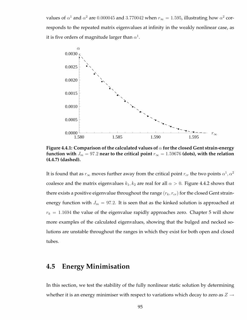
values of α1 and α2 are 0.000045 and 3.770042 when r∞ = 1.595, illustrating how α2 cor-

responds to the repeated matrix eigenvalues at infinity in the weakly nonlinear case, as

it is five orders of magnitude larger than α1.

1.580 1.585 1.590 1.5950.0000

0.0005

0.0010

0.0015

0.0020

0.0025

0.0030

r∞

α

Figure 4.4.1: Comparison of the calculated values of α for the closed Gent strain-energyfunction with Jm = 97.2 near to the critical point r∞ = 1.59676 (dots), with the relation(4.4.7) (dashed).

It is found that as r∞ moves further away from the critical point rcr the two points α1, α2

coalesce and the matrix eigenvalues k1, k2 are real for all α > 0. Figure 4.4.2 shows that

there exists a positive eigenvalue throughout the range (rk, rcr) for the closed Gent strain-

energy function with Jm = 97.2. It is seen that as the kinked solution is approached at

rk = 1.1694 the value of the eigenvalue rapidly approaches zero. Chapter 5 will show

more examples of the calculated eigenvalues, showing that the bulged and necked so-

lutions are unstable throughout the ranges in which they exist for both open and closed

tubes.

4.5 Energy Minimisation

In this section, we test the stability of the fully nonlinear static solution by determining

whether it is an energy minimiser with respect to variations which decay to zero as Z →

95

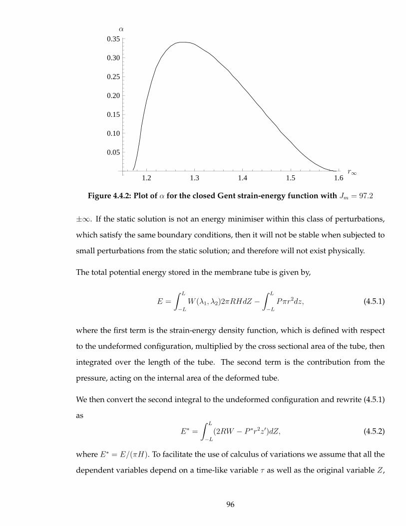
1.2 1.3 1.4 1.5 1.6

0.05

0.10

0.15

0.20

0.25

0.30

0.35

r∞

α

Figure 4.4.2: Plot of α for the closed Gent strain-energy function with Jm = 97.2

±∞. If the static solution is not an energy minimiser within this class of perturbations,

which satisfy the same boundary conditions, then it will not be stable when subjected to

small perturbations from the static solution; and therefore will not exist physically.

The total potential energy stored in the membrane tube is given by,

E =

∫ L

−L

W (λ1, λ2)2πRHdZ −∫ L

−L

Pπr2dz, (4.5.1)

where the first term is the strain-energy density function, which is defined with respect

to the undeformed configuration, multiplied by the cross sectional area of the tube, then

integrated over the length of the tube. The second term is the contribution from the

pressure, acting on the internal area of the deformed tube.

We then convert the second integral to the undeformed configuration and rewrite (4.5.1)

as

E∗ =

∫ L

−L

(2RW − P ∗r2z′)dZ, (4.5.2)

where E∗ = E/(πH). To facilitate the use of calculus of variations we assume that all the

dependent variables depend on a time-like variable τ as well as the original variable Z,

96

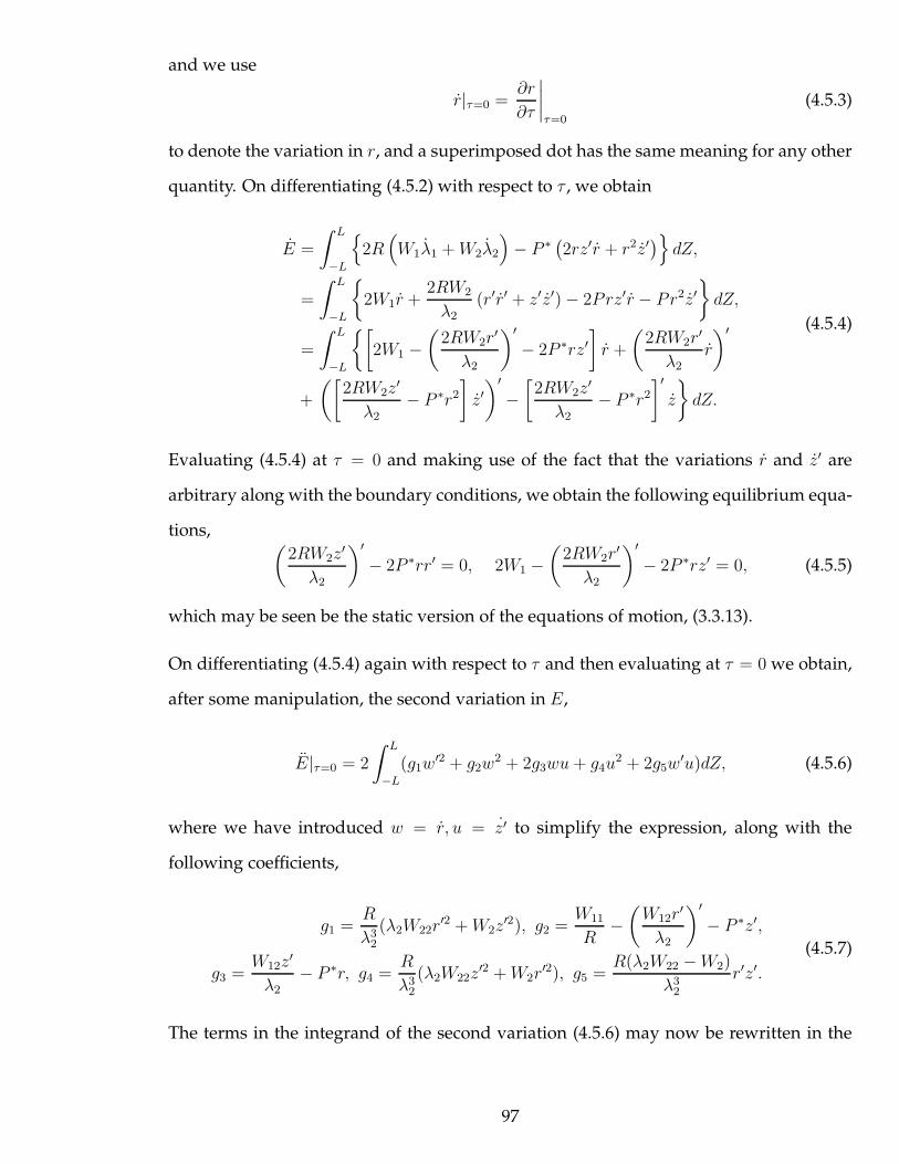
and we use

r|τ=0 =∂r

∂τ

∣∣∣∣τ=0

(4.5.3)

to denote the variation in r, and a superimposed dot has the same meaning for any other

quantity. On differentiating (4.5.2) with respect to τ , we obtain

E =

∫ L

−L

{

2R(

W1λ1 +W2λ2

)

− P ∗(2rz′r + r2z′

)}

dZ,

=

∫ L

−L

{

2W1r +2RW2

λ2(r′r′ + z′z′) − 2Prz′r − Pr2z′

}

dZ,

=

∫ L

−L

{[

2W1 −(

2RW2r′

λ2

)′

− 2P ∗rz′]

r +

(2RW2r

′

λ2r

)′

+

([2RW2z

′

λ2− P ∗r2

]

z′)′

−[2RW2z

′

λ2− P ∗r2

]′

z

}

dZ.

(4.5.4)

Evaluating (4.5.4) at τ = 0 and making use of the fact that the variations r and z′ are

arbitrary along with the boundary conditions, we obtain the following equilibrium equa-

tions,(

2RW2z′

λ2

)′

− 2P ∗rr′ = 0, 2W1 −(

2RW2r′

λ2

)′

− 2P ∗rz′ = 0, (4.5.5)

which may be seen be the static version of the equations of motion, (3.3.13).

On differentiating (4.5.4) again with respect to τ and then evaluating at τ = 0 we obtain,

after some manipulation, the second variation in E,

E|τ=0 = 2

∫ L

−L

(g1w′2 + g2w

2 + 2g3wu+ g4u2 + 2g5w

′u)dZ, (4.5.6)

where we have introduced w = r, u = z′ to simplify the expression, along with the

following coefficients,

g1 =R

λ32

(λ2W22r′2 +W2z

′2), g2 =W11

R−(W12r

′

λ2

)′

− P ∗z′,

g3 =W12z

′

λ2− P ∗r, g4 =

R

λ32

(λ2W22z′2 +W2r

′2), g5 =R(λ2W22 −W2)

λ32

r′z′.

(4.5.7)

The terms in the integrand of the second variation (4.5.6) may now be rewritten in the

97

following way, as

E|τ=0 = 2

∫ L

−L

{(√a1w

′ +g5√g1

u

)2

+ g2w2 + 2g3wu+

(

g4 −g25

g1

)

u2

}

dZ

= 2

∫ L

−L

{(√g1w

′ +g5√g1u

)2

+ v · G(Z)vT

}

dZ, (4.5.8)

where v = (w, u), and

G(Z) =

g2 g3

g3 g4 − g25/g1

. (4.5.9)

It can be immediately deduced that a sufficient condition for the positive semi-definiteness

of the second variation of the potential energy is that G is positive semi-definite for all

Z, where a matrix G is positive semi-definite if x.G.x ≥ 0 for all non-zero vectors x. It

may also be shown, using proof by contradiction with an appropriate choice of variations

(w, u), that this condition is also necessary (Y.B. Fu, personal communication, 6th April

2009). We thus conclude that if G is positive semi-definite for all Z for a given r, z, then

the corresponding equilibrium solution is an energy minimiser.

An equivalent statement to G being positive semi-definite is that both of the eigenval-

ues of G are non-negative. We may therefore test the stability just from considering the

eigenvalues of G, over the range of Z. We let ρ(Z) be the smallest eigenvalue of G, at

a given Z. For many bulged or necked solutions, it is only necessary to evaluate the

eigenvalues of G at Z = 0, as one of the eigenvalues is negative as shown in Figure 4.5.1.

As the critical point rcr = 1.59 in Figure 4.5.1 is approached, ρ(0) approaches zero with

ρ(Z) > 0 for the remaining range of Z. As the kinked solution rk = 1.1674 is approached,

ρ(0) becomes positive, although there is a range of Z during which ρ(Z) is still negative

as may be seen in Figure 4.5.2. This is expected as around the origin the uniform state

associated with the kink at Z = 0 is being approached which is stable as discussed above,

and it is therefore only the nonuniform transition region which may be unstable. As the

kink is approached further, this small range of Z in which ρ(Z) < 0 moves away from

98

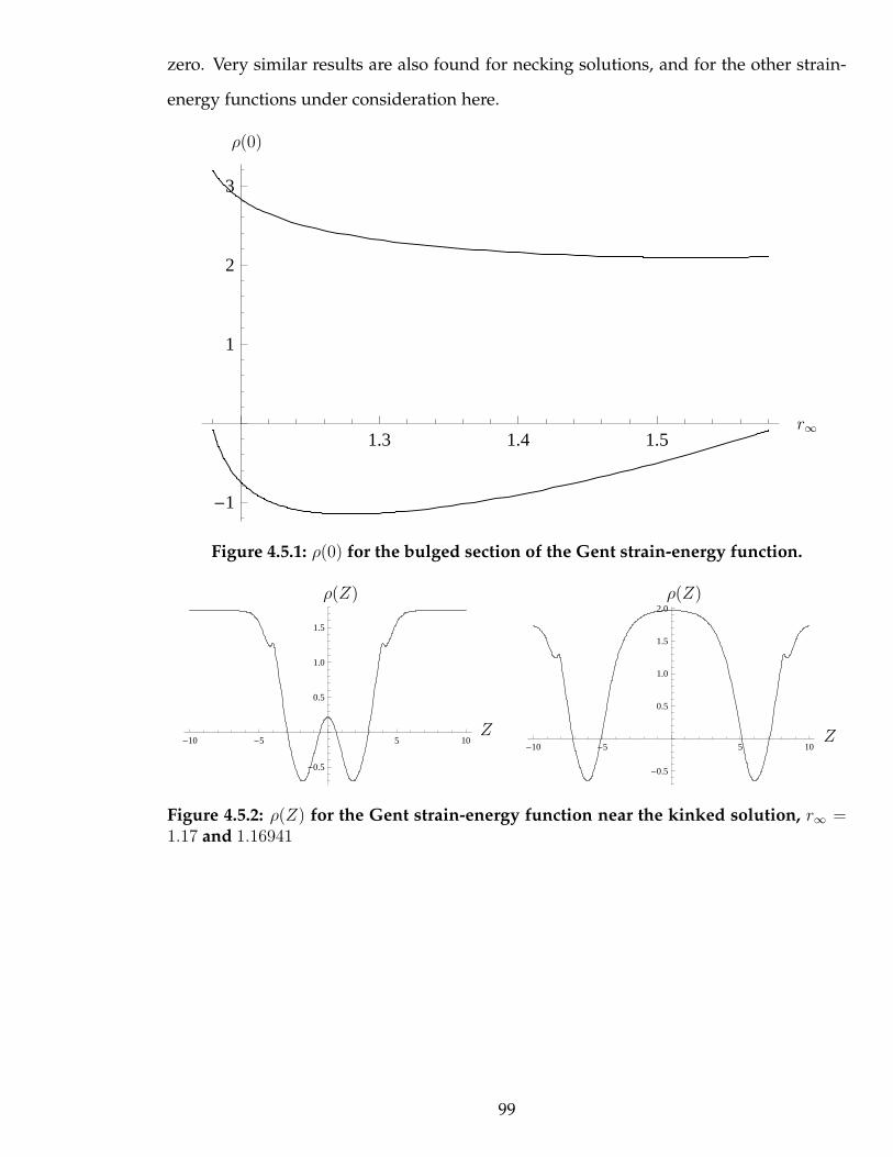
zero. Very similar results are also found for necking solutions, and for the other strain-

energy functions under consideration here.

1.3 1.4 1.5

-1

1

2

3

r∞

ρ(0)

Figure 4.5.1: ρ(0) for the bulged section of the Gent strain-energy function.

-10 -5 5 10

-0.5

0.5

1.0

1.5

Z

ρ(Z)

-10 -5 5 10

-0.5

0.5

1.0

1.5

2.0

Z

ρ(Z)

Figure 4.5.2: ρ(Z) for the Gent strain-energy function near the kinked solution, r∞ =1.17 and 1.16941

99

4.6 Conclusion

Both the spectral stability and energy methods have shown that the solitary wave type

solutions, in either the bulged or necked case, are unstable with respect to axisymmetric

perturbations when the internal pressure is controlled. The analysis suggests that the

kinked type solution is stable as the eigenvalue tends towards zero as the kinked solution

is approached in the spectral stability test. What can be said for the kinked case is that,

as the first bifurcation must be subcritical and the second supercritical, the two uniform

states which the kinked solution consists of must both be stable; as may be seen from

the projections onto the r0 = r∞ line of the points E and G in Figure 3.5.1(b). Therefore

it is just the transition region which may cause instability, as seen in the energy method

above.

Experience with rubber modelling balloons suggests that when inflated the bulged state

is unstable but the kinked state is stable and observable, indeed this was a motivating ex-

ample for the considerations here. The experiments by Alexander (1971) and Kyriakides

and Chang (1990, 1991), also appear to suggest that the kinked state is stable as it is ob-

served. We therefore tentatively suggest that the kinked solution is stable, although we

are unable to prove this to be true.

100

Chapter 5

Comparison of Strain-Energy Functions

5.1 Introduction

In this chapter we use the results from Chapters 3 and 4 to determine the inflation of

the cylindrical membrane for various strain-energy functions with both closed and open

ends, including varying the axial pre-stretch z∞ in the case of open ends. The bifurcation

condition ω(r∞) is calculated, as well as the amplitude stretch diagram discussed in Sec-

tion 3.5, for the different strain-energy functions. In addition, we show the eigenvalues

found via the stability test detailed in Chapter 4.

5.2 Varga Strain-Energy Function

5.2.1 Bifurcation Condition

Initially we will derive results for the Varga strain-energy function given by (2.2.10). The

simple form of this strain-energy function allows us to solve (3.3.21) and (3.3.22) explic-

itly to find r0 and z′0. Equation (3.3.22) can be solved to express z′0 in terms of r0, and then

101

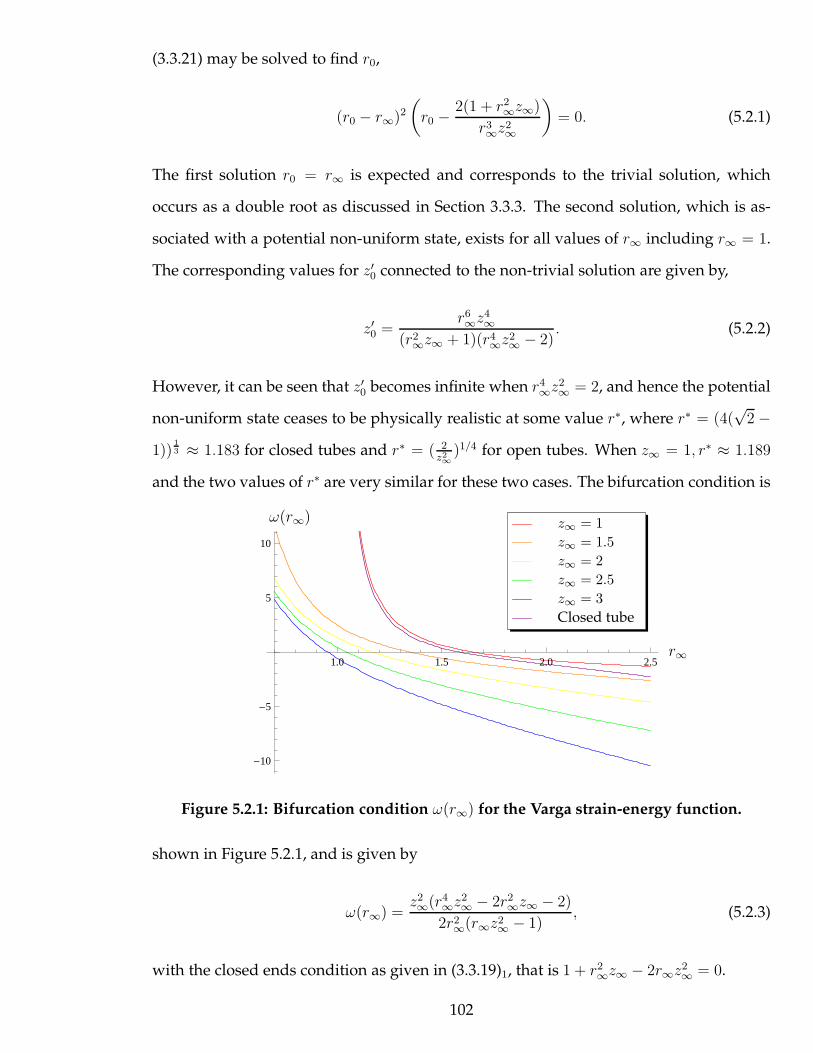
(3.3.21) may be solved to find r0,

(r0 − r∞)2

(

r0 −2(1 + r2

∞z∞)

r3∞z

2∞

)

= 0. (5.2.1)

The first solution r0 = r∞ is expected and corresponds to the trivial solution, which

occurs as a double root as discussed in Section 3.3.3. The second solution, which is as-

sociated with a potential non-uniform state, exists for all values of r∞ including r∞ = 1.

The corresponding values for z′0 connected to the non-trivial solution are given by,

z′0 =r6∞z

4∞

(r2∞z∞ + 1)(r4

∞z2∞ − 2)

. (5.2.2)

However, it can be seen that z′0 becomes infinite when r4∞z

2∞ = 2, and hence the potential

non-uniform state ceases to be physically realistic at some value r∗, where r∗ = (4(√

2 −

1))13 ≈ 1.183 for closed tubes and r∗ = ( 2

z2∞

)1/4 for open tubes. When z∞ = 1, r∗ ≈ 1.189

and the two values of r∗ are very similar for these two cases. The bifurcation condition is

1.0 1.5 2.0 2.5

-10

-5

5

10

r∞

ω(r∞)z∞ = 1

z∞ = 1.5

z∞ = 2

z∞ = 2.5

z∞ = 3

Closed tube

Figure 5.2.1: Bifurcation condition ω(r∞) for the Varga strain-energy function.

shown in Figure 5.2.1, and is given by

ω(r∞) =z2∞(r4

∞z2∞ − 2r2

∞z∞ − 2)

2r2∞(r∞z2

∞ − 1), (5.2.3)

with the closed ends condition as given in (3.3.19)1, that is 1 + r2∞z∞ − 2r∞z

2∞ = 0.

102

For open ended tubes, the bifurcation point is therefore found by solving the quartic in

the numerator of (5.2.3), giving rcr =√

1+√

3z∞

. For the closed tube we need to solve the

two equations simultaneously, giving r∞ = 22/3, z∞ = 2−4/3(1+√

3), which is close to the

result for z∞ = 1 as seen in Figure 5.2.1. Obviously, if the remote axial stretch z∞ is greater

than 1+√

3 then the critical point comes before unity, indicating that a large axial stretch is

associated with a reduction in the far-radius. In the case where z∞ < 1, the denominator

of (5.2.3) can become infinite and hence ω(r∞) tend to zero for some r∞ > 1, but we

require that z∞ > 1 as the membrane is in tension rather than compression. Therefore,

for open ends r∗ is related to the critical point rcr by,

r∗ =4√

2√

1 +√

3rcr ≈ 0.7194rcr, (5.2.4)

implying that, for all values of the remote axial stretch, there is a range of r∞ for which a

bulged tube may exist.

5.2.2 Amplitude-Stretch Diagram

The amplitude-stretch diagrams for a variety of z∞ along with the case of closed ends, are

given in Figure 5.2.2, which shows how the amplitude of the potential bifurcated solution

behaves as r∞ is changed. Figure 5.2.2 corresponds to the non-trivial solution of (5.2.1),

and shows the amplitude of the bulged solutions. The existence of the bulged solutions

indicated in Figure 5.2.2 is shown by the negative gradient of ω(rcr) in Figure 5.2.1, for

the various z∞. The abrupt ends of the top curves represent r∗, where z′0 becomes infinite

and show that the values of r0 at which this occurs are finite. Past this point the curves

continue in the same manner but with negative z′0, and are therefore not shown after this

point. The case of closed ends is quantitatively similar to that of the open ends, with the

effect of the variation in z∞ clearly shown, as it varies between the curves for z∞ = 1 and

z∞ = 1.5. As r∗ is approached z′0 tends to infinity, leading to a deformed configuration

which flattens at Z = 0, in a similar way to the kinked solutions, as shown in Figure 5.2.3.

103

1.0 1.5 2.0 2.5

-2

-1

0

1

r∞

r0 − r∞ z∞ = 1

z∞ = 1.5

z∞ = 2

z∞ = 2.5

z∞ = 3

Closed tube

Figure 5.2.2: Potential bulge/neck amplitude r0 − r∞ for the Varga strain-energy func-tion.

-3 -2 -1 0 1 2 3

1.5

2.0

2.5

-3 -2 -1 0 1 2 3

1.5

2.0

2.5

z(Z)

r(Z)

r∞ = 1.187

r∞ = 1.22

r∞ = 1.25

r∞ = 1.3

r∞ = 1.4

Z

r(Z)

Figure 5.2.3: Plots of r against Z and z for the closed Varga tube as r∗ is approached.

However, this is a separate mechanism than that which leads to the kinked solutions

detailed in Section 3.6 as those solutions do not become infinite.

In addition, equation (3.4.4) may be written analytically as,

r′2 =4z2

∞(r2∞(ψ2r − 4r2

∞z2∞)2 − r(r2 + r2

∞ + r4∞z∞ − r2

∞z∞r2 − 2r3

∞z2∞)2)

ψ2r2(ψ2r − 4r2∞z

2∞)2

, (5.2.5)

where ψ = 2 + r∞z∞(r∞ − r). Equation (5.2.5) may be solved subject to the second initial

condition in (5.2.1), to obtain a bounded non-uniform solution for r(Z) for all values of

104

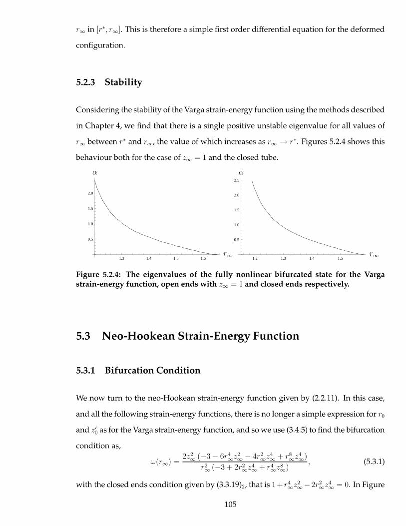
r∞ in [r∗, r∞]. This is therefore a simple first order differential equation for the deformed

configuration.

5.2.3 Stability

Considering the stability of the Varga strain-energy function using the methods described

in Chapter 4, we find that there is a single positive unstable eigenvalue for all values of

r∞ between r∗ and rcr, the value of which increases as r∞ → r∗. Figures 5.2.4 shows this

behaviour both for the case of z∞ = 1 and the closed tube.

1.3 1.4 1.5 1.6

0.5

1.0

1.5

2.0

r∞

α

1.2 1.3 1.4 1.5

0.5

1.0

1.5

2.0

2.5

r∞

α

Figure 5.2.4: The eigenvalues of the fully nonlinear bifurcated state for the Vargastrain-energy function, open ends with z∞ = 1 and closed ends respectively.

5.3 Neo-Hookean Strain-Energy Function

5.3.1 Bifurcation Condition

We now turn to the neo-Hookean strain-energy function given by (2.2.11). In this case,

and all the following strain-energy functions, there is no longer a simple expression for r0

and z′0 as for the Varga strain-energy function, and so we use (3.4.5) to find the bifurcation

condition as,

ω(r∞) =2z2

∞ (−3 − 6r4∞z

2∞ − 4r2

∞z4∞ + r8

∞z4∞)

r2∞ (−3 + 2r2

∞z4∞ + r4

∞z8∞)

, (5.3.1)

with the closed ends condition given by (3.3.19)2, that is 1+ r4∞z

2∞−2r2

∞z4∞ = 0. In Figure

105

1.0 1.5 2.0 2.5

-4

-2

2

4

r∞

ω(r∞)z∞ = 1

z∞ = 1.5

z∞ = 2

z∞ = 2.5

z∞ = 3

Closed tube

Figure 5.3.1: Bifurcation condition ω(r∞) for the neo-Hookean strain-energy function.

5.3.1 the bifurcation condition (5.3.1) is plotted for a range of z∞ along with the closed

ends case. In the limit as z∞ → ∞ the bifurcation point rcr approaches 213 from above.

Thus there exists a critical point at all values of z∞ > 0, in the same way as for the Varga

strain-energy function, but in this case it is always greater than unity.

5.3.2 Amplitude-Stretch Diagram

1.0 1.5 2.0 2.5

-2

-1

0

1

2

3

4

5

r∞

r0 − r∞ z∞ = 1

z∞ = 1.5

z∞ = 2

z∞ = 2.5

z∞ = 3

Closed tube

Figure 5.3.2: Potential bulge/neck amplitude r0−r∞ for the neo-Hookean strain-energyfunction.

In addition, there exists a limit point r∗ = (z∞)12 similarly to the Varga strain-energy

106

function, at which r0 and z′0 both become infinite, which may be seen in the amplitude-

stretch diagram shown in Figure 5.3.2. This corresponds to a singularity in that the tube

keeps expanding indefinitely, presumably followed by rupture. The case of closed ends

has the singularity at r∗ = 1 and the bifurcation point at rcr = (17 + 3√

21)1/6/2.

5.4 Gent Strain-Energy Function

5.4.1 Bifurcation Condition

We now consider the Gent strain-energy function given by (2.2.13), which was used as

the prevailing example throughout the derivations given in Chapter 3. The parameter

Jm, which represents the maximum stretch which the molecular chains comprising the

material can extend to as detailed in Section 2.2.4, will be shown as 30 or 97.2 in these

examples, although very similar qualitative behaviour is found across the range of Jm,

with the diagram being compressed for smaller Jm. The bifurcation condition (3.4.5) is

2 4 6 8 10

-20

-10

10

20

r∞

ω(r∞) z∞ = 1

z∞ = 1.5

z∞ = 2

z∞ = 2.5

z∞ = 3

Closed tube

Figure 5.4.1: Bifurcation condition for the Gent strain-energy function with Jm = 97.2

given by a sixth order polynomial in r2∞, which must be solved numerically. Figure 5.4.1

107

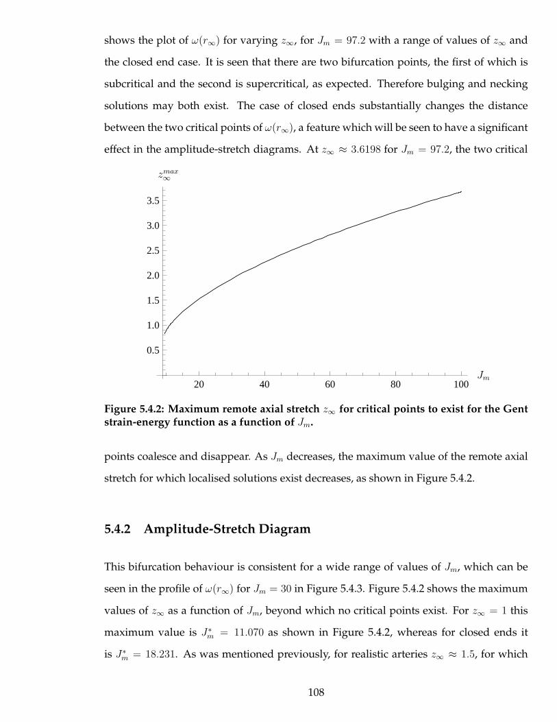
shows the plot of ω(r∞) for varying z∞, for Jm = 97.2 with a range of values of z∞ and

the closed end case. It is seen that there are two bifurcation points, the first of which is

subcritical and the second is supercritical, as expected. Therefore bulging and necking

solutions may both exist. The case of closed ends substantially changes the distance

between the two critical points of ω(r∞), a feature which will be seen to have a significant

effect in the amplitude-stretch diagrams. At z∞ ≈ 3.6198 for Jm = 97.2, the two critical

20 40 60 80 100

0.5

1.0

1.5

2.0

2.5

3.0

3.5

Jm

zmax∞

Figure 5.4.2: Maximum remote axial stretch z∞ for critical points to exist for the Gentstrain-energy function as a function of Jm.

points coalesce and disappear. As Jm decreases, the maximum value of the remote axial

stretch for which localised solutions exist decreases, as shown in Figure 5.4.2.

5.4.2 Amplitude-Stretch Diagram

This bifurcation behaviour is consistent for a wide range of values of Jm, which can be

seen in the profile of ω(r∞) for Jm = 30 in Figure 5.4.3. Figure 5.4.2 shows the maximum

values of z∞ as a function of Jm, beyond which no critical points exist. For z∞ = 1 this

maximum value is J∗m = 11.070 as shown in Figure 5.4.2, whereas for closed ends it

is J∗m = 18.231. As was mentioned previously, for realistic arteries z∞ ≈ 1.5, for which

108

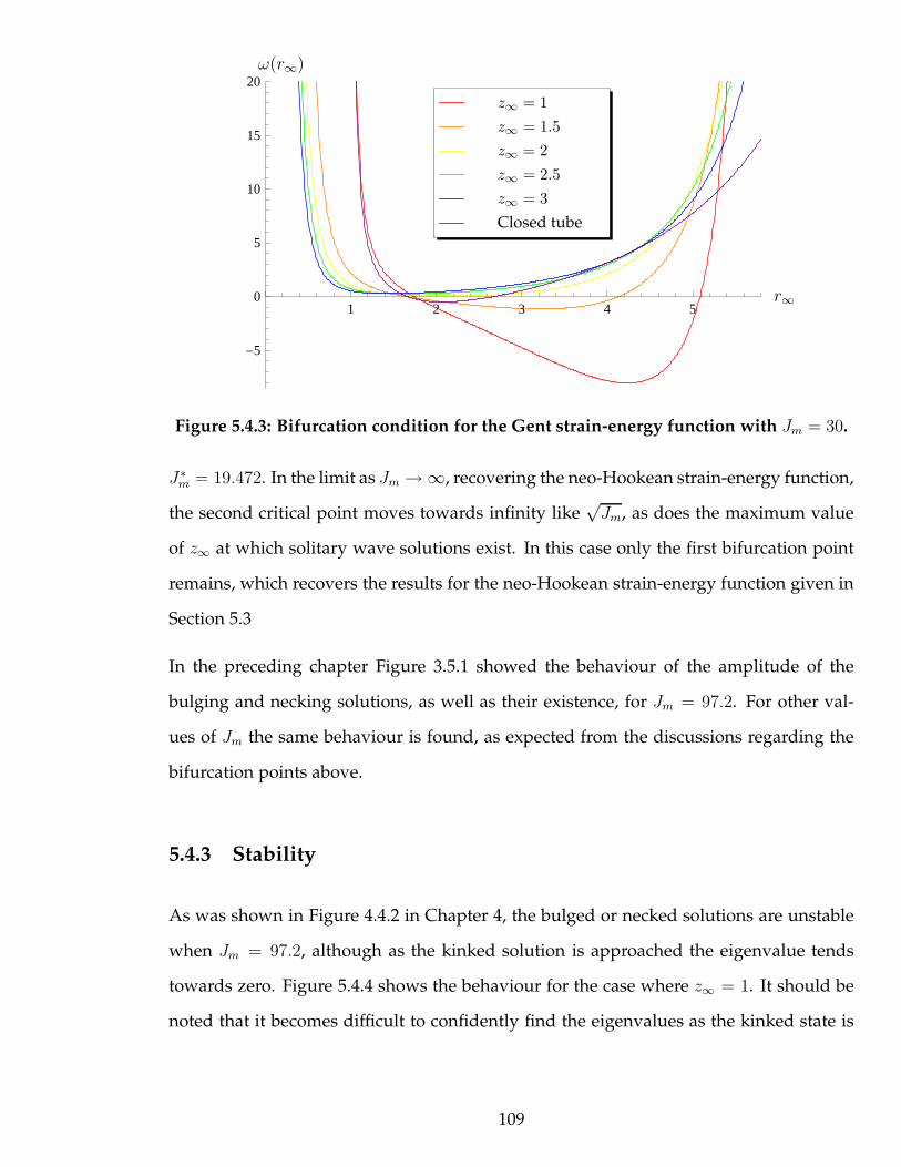
1 2 3 4 5

-5

0

5

10

15

20

r∞

ω(r∞)

z∞ = 1

z∞ = 1.5

z∞ = 2

z∞ = 2.5

z∞ = 3

Closed tube

Figure 5.4.3: Bifurcation condition for the Gent strain-energy function with Jm = 30.

J∗m = 19.472. In the limit as Jm → ∞, recovering the neo-Hookean strain-energy function,

the second critical point moves towards infinity like√Jm, as does the maximum value

of z∞ at which solitary wave solutions exist. In this case only the first bifurcation point

remains, which recovers the results for the neo-Hookean strain-energy function given in

Section 5.3

In the preceding chapter Figure 3.5.1 showed the behaviour of the amplitude of the

bulging and necking solutions, as well as their existence, for Jm = 97.2. For other val-

ues of Jm the same behaviour is found, as expected from the discussions regarding the

bifurcation points above.

5.4.3 Stability

As was shown in Figure 4.4.2 in Chapter 4, the bulged or necked solutions are unstable

when Jm = 97.2, although as the kinked solution is approached the eigenvalue tends

towards zero. Figure 5.4.4 shows the behaviour for the case where z∞ = 1. It should be

noted that it becomes difficult to confidently find the eigenvalues as the kinked state is

109

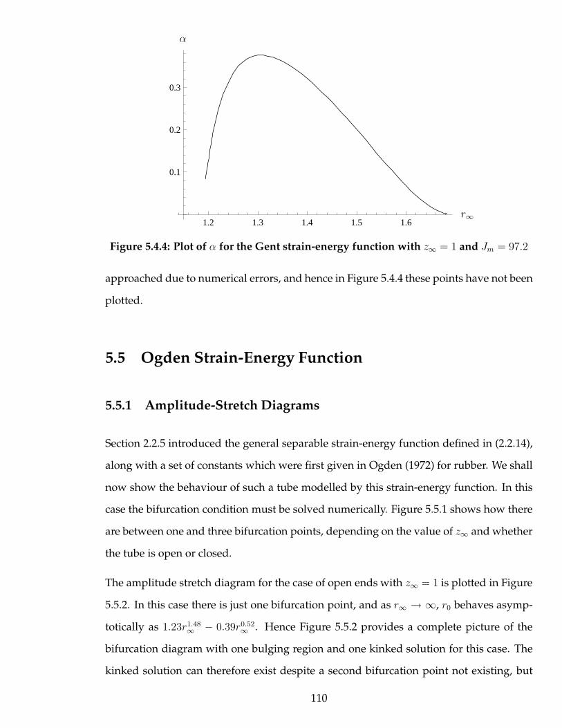
1.2 1.3 1.4 1.5 1.6

0.1

0.2

0.3

r∞

α

Figure 5.4.4: Plot of α for the Gent strain-energy function with z∞ = 1 and Jm = 97.2

approached due to numerical errors, and hence in Figure 5.4.4 these points have not been

plotted.

5.5 Ogden Strain-Energy Function

5.5.1 Amplitude-Stretch Diagrams

Section 2.2.5 introduced the general separable strain-energy function defined in (2.2.14),

along with a set of constants which were first given in Ogden (1972) for rubber. We shall

now show the behaviour of such a tube modelled by this strain-energy function. In this

case the bifurcation condition must be solved numerically. Figure 5.5.1 shows how there

are between one and three bifurcation points, depending on the value of z∞ and whether

the tube is open or closed.

The amplitude stretch diagram for the case of open ends with z∞ = 1 is plotted in Figure

5.5.2. In this case there is just one bifurcation point, and as r∞ → ∞, r0 behaves asymp-

totically as 1.23r1.48∞ − 0.39r0.52

∞ . Hence Figure 5.5.2 provides a complete picture of the

bifurcation diagram with one bulging region and one kinked solution for this case. The

kinked solution can therefore exist despite a second bifurcation point not existing, but

110

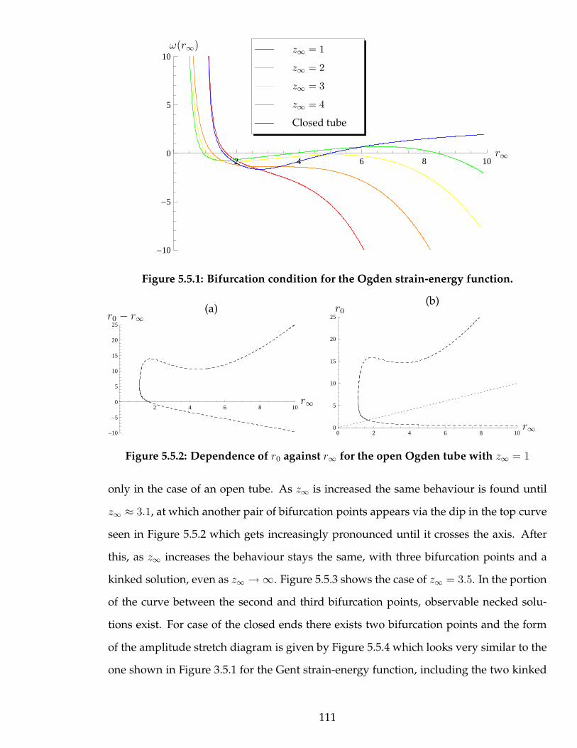
2 4 6 8 10

-10

-5

0

5

10

r∞

ω(r∞)z∞ = 1

z∞ = 2

z∞ = 3

z∞ = 4

Closed tube

Figure 5.5.1: Bifurcation condition for the Ogden strain-energy function.

2 4 6 8 10

-10

-5

0

5

10

15

20

25

r∞

r0 − r∞(a)

0 2 4 6 8 100

5

10

15

20

25

r∞

r0(b)

Figure 5.5.2: Dependence of r0 against r∞ for the open Ogden tube with z∞ = 1

only in the case of an open tube. As z∞ is increased the same behaviour is found until

z∞ ≈ 3.1, at which another pair of bifurcation points appears via the dip in the top curve

seen in Figure 5.5.2 which gets increasingly pronounced until it crosses the axis. After

this, as z∞ increases the behaviour stays the same, with three bifurcation points and a

kinked solution, even as z∞ → ∞. Figure 5.5.3 shows the case of z∞ = 3.5. In the portion

of the curve between the second and third bifurcation points, observable necked solu-

tions exist. For case of the closed ends there exists two bifurcation points and the form

of the amplitude stretch diagram is given by Figure 5.5.4 which looks very similar to the

one shown in Figure 3.5.1 for the Gent strain-energy function, including the two kinked

111

2 4 6 8 10

-10

-5

5

r∞

r0 − r∞

0 2 4 6 8 100

2

4

6

8

10

r∞

r0

Figure 5.5.3: Dependence of r0 against r∞ for the open Ogden tube with z∞ = 3.5,dashed lines represent non-observable solutions.

1 2 3 4 5 6 7

-5

0

5

10

A

B

DF r∞

r0 − r∞(a)

1 2 3 4 5 6

1

2

3

4

5

6

A

BC

D

E

F

G

r∞

r0(b)

Figure 5.5.4: Dependence of r0 against r∞ for the closed Ogden tube. Only the solidlines in (a) correspond to localised solutions, and the non-localised solutions are notplotted in (b)

solutions. The labels A− G on 5.5.4 correspond exactly to those discussed in Section 3.5

for the Gent strain-energy function, and the behaviour is the same. The behaviour for

this Ogden strain-energy function is therefore dependent on the boundary conditions,

changing whether there exists one, two or three critical points.

112

5.5.2 Stability

1.2 1.3 1.4 1.5 1.6

0.1

0.2

0.3

0.4

0.5

0.6

r∞

α

Figure 5.5.5: Plot of α for the open tube with the Ogden strain-energy function.

Again, using the methods in Section 4.4, we show that there exists a positive eigenvalue

of the spectral stability test and the bulged solution is therefore unstable, as given in

Figure 5.5.5, which looks very similar to that in Figure 4.4.2 for the Gent strain-energy

function with Jm = 97.2.

5.6 Fung Strain-Energy Function

We now consider the Fung strain-energy function described by (2.2.15) which includes

a parameter Γ > 0 representing the amount of strain stiffening of the material. For a

tube with open ends if Γ > Γo = 0.166 then no bifurcation points exist for any z∞ ≥ 1.

For values of Γ less than Γo, then a single bifurcation point exists for values of z∞ close

to one, with very similar behaviour as the neo-Hookean strain-energy function. This is

expected, as when Γ = 0 the neo-Hookean model is recovered. As Γ increases towards Γc,

the bifurcation point rcr moves towards infinity. When a closed end tube is considered,

for small Γ < Γc = 0.065 there exists two bifurcation points and two kinked solutions

113

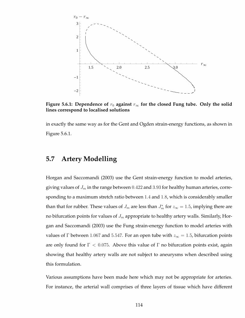
1.5 2.0 2.5 3.0

-2

-1

1

2

3

r∞

r0 − r∞

Figure 5.6.1: Dependence of r0 against r∞ for the closed Fung tube. Only the solidlines correspond to localised solutions

in exactly the same way as for the Gent and Ogden strain-energy functions, as shown in

Figure 5.6.1.

5.7 Artery Modelling

Horgan and Saccomandi (2003) use the Gent strain-energy function to model arteries,

giving values of Jm in the range between 0.422 and 3.93 for healthy human arteries, corre-

sponding to a maximum stretch ratio between 1.4 and 1.8, which is considerably smaller

than that for rubber. These values of Jm are less than J∗m for z∞ = 1.5, implying there are

no bifurcation points for values of Jm appropriate to healthy artery walls. Similarly, Hor-

gan and Saccomandi (2003) use the Fung strain-energy function to model arteries with

values of Γ between 1.067 and 5.547. For an open tube with z∞ = 1.5, bifurcation points

are only found for Γ < 0.075. Above this value of Γ no bifurcation points exist, again

showing that healthy artery walls are not subject to aneurysms when described using

this formulation.

Various assumptions have been made here which may not be appropriate for arteries.

For instance, the arterial wall comprises of three layers of tissue which have different

114

properties (Humphrey 2003). In addition, there are collagen fibres inside the arterial

wall which, due to their relative stiffness compared to the elastic tissues, induce pre-

ferred directions of stretch into the artery walls (Holzapfel et al. 2000). Hence arteries

are anisotropic in their deformations and require an anisotropic strain-energy function,

as discussed in Horgan and Saccomandi (2003) for example. Similarly, Fung (1993) gives

evidence of arterial walls being viscoelastic in their response to stress and strain. Another

issue discussed by Alastrue et al. (2007) is that the arteries are not unstressed in the refer-

ence configuration, so the existence of this pre-stress may also be a factor in the existence

of aneurysms. This problem is also considered by Gee et al. (2009) for finite-element

simulations of arteries. In order to include such a pre-stress the wall thickness has to be

assumed to be non-trivial, consequently the membrane assumption can not be used and

another approach is required. Studies on thick-walled elastic tubes include Haughton

and Ogden (1979b) and Zhu et al. (2008). In addition to these considerations, aneurysms

also combine elements of growth and remodelling over time and therefore these factors

need to be incorporated.

5.8 Conclusion

It has been shown that, for a range of strain-energy functions, bulging or necking solu-

tions may exist. As expected and discussed in Section 4.2, the first bifurcation point, if

it exists, has been shown to always be subcritical due to the stability of the undeformed

tube, followed by a supercritical bifurcation point if a second exists. The comparison of

several strain-energy functions shows how the existence and behaviour of non-uniform

solutions varies depending on the choice of strain-energy function and the conditions

imposed at infinity. In particular, when the tube has closed ends a closed curve may

occur in the r0 − r∞ plane, connecting two kinked solutions and two bifurcation points,

with the interpretation given in Section 3.6.

115

Chapter 6

Inflation of a Spherical Membrane

6.1 Introduction

In this section we take the foundations of the boundary value problem studied for the

isotropic, incompressible, homogenous elastic cylindrical membrane and apply them to

the case of an initially spherical membrane. It is assumed that there is an internal pressure

uniformly inflating the sphere, which is the controlling parameter for the deformation,

and we again aim to find non-uniform solutions to this deformation.

In accordance with Chapter 3, we only consider deformations which are axisymmetric

around the Z axis, and we continue to use cylindrical polar coordinates instead of intro-

ducing spherical polar coordinates in order to facilitate this. This derivation follows the

configuration introduced in Haughton (1980), although relabelling the 1 and 2 directions

to coincide with those used in Chapter 3. In particular we are interested in axisymmetric

modes superimposed upon the spherically symmetric solution. Physical applications of

this mathematical deformation include the inflation of spherical rubber balloons, osmotic

swelling of animal cells and imbibition (initial water uptake) of germinating plant seeds.

Gent (2005) and Kanner and Horgan (2007) discuss how the spherical inflation has a

limit-point instability in the same way as the cylindrical tube, which occurs at the maxi-

mum of the pressure-volume diagram of the radially symmetric inflated sphere.

116

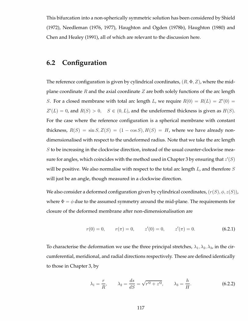
This bifurcation into a non-spherically symmetric solution has been considered by Shield

(1972), Needleman (1976, 1977), Haughton and Ogden (1978b), Haughton (1980) and

Chen and Healey (1991), all of which are relevant to the discussion here.

6.2 Configuration

The reference configuration is given by cylindrical coordinates, (R,Φ, Z), where the mid-

plane coordinate R and the axial coordinate Z are both solely functions of the arc length

S. For a closed membrane with total arc length L, we require R(0) = R(L) = Z ′(0) =

Z ′(L) = 0, and R(S) > 0, S ∈ (0, L), and the undeformed thickness is given as H(S).

For the case where the reference configuration is a spherical membrane with constant

thickness, R(S) = sinS, Z(S) = (1 − cosS), H(S) = H , where we have already non-

dimensionalised with respect to the undeformed radius. Note that we take the arc length

S to be increasing in the clockwise direction, instead of the usual counter-clockwise mea-

sure for angles, which coincides with the method used in Chapter 3 by ensuring that z′(S)

will be positive. We also normalise with respect to the total arc length L, and therefore S

will just be an angle, though measured in a clockwise direction.

We also consider a deformed configuration given by cylindrical coordinates, (r(S), φ, z(S)),

where Φ = φ due to the assumed symmetry around the mid-plane. The requirements for

closure of the deformed membrane after non-dimensionalisation are

r(0) = 0, r(π) = 0, z′(0) = 0, z′(π) = 0. (6.2.1)

To characterise the deformation we use the three principal stretches, λ1, λ2, λ3, in the cir-

cumferential, meridional, and radial directions respectively. These are defined identically

to those in Chapter 3, by

λ1 =r

R, λ2 =

ds

dS=

√r′2 + z′2, λ3 =

h

H. (6.2.2)

117

The material is assumed to be incompressible and hence λ1λ2λ3 = 1. The only difference

which should be noted is that R is now a function of S rather than a constant. Note

that Haughton (1980), as do many other authors, reverses the labelling of the first two

principal stretches, but we choose to be consistent with Chapter 3.

At the two poles of the membrane, both of the circumferential and meridional stretches

become,

limS→0

λ1(S) = r′(0), limS→0

λ2(S) = r′(0), (6.2.3)

and similarly around S = π, where it is noted that r′(0) ≥ 0, r′(π) ≤ 0 as the deformed

radius must be increasing away from the poles.

The equilibrium equations, written in terms of the principal stretches, λi and the principal

Cauchy stresses, σi, are given by (Haughton 1980),

(hrσ2)′ − hr′σ1 = 0 (6.2.4)

z′σ1

rλ2

+ σ2(r′z′′ − r′′z′)

λ32

− P ∗

λ3

= 0, (6.2.5)

where a superimposed prime denotes differentiation with respect to S, and P ∗ = P/H .

We note that (6.2.4) and (6.2.5) reduce to the same equilibrium equations as for the cylin-

drical membrane discussed in Chapter 3, but for a non-constant R. In addition, by the

same method as described in Chapter 3, they may be derived using a perturbation ex-

pansion from the equilibrium equation (2.1.41) by expanding in the thickness coordinate

through the membrane.

By introducing the principal curvatures of the membrane as

κ1 =z′

rλ2, κ2 =

(r′z′′ − r′′z′)

λ32

=1

r′

(z′

λ2

)′

=−1

z′

(r′

λ2

)′

, (6.2.6)

equation (6.2.5) may be written as,

κ1σ1 + κ2σ2 − P ∗λ1λ2 = 0. (6.2.7)

118

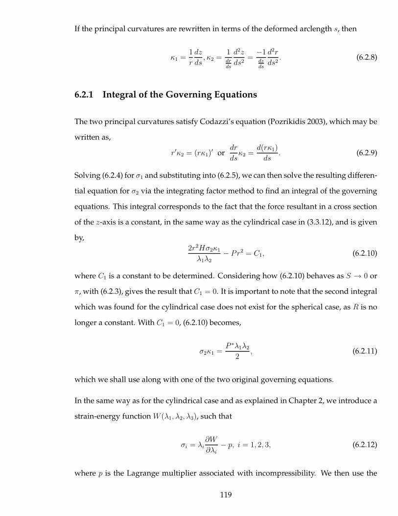
If the principal curvatures are rewritten in terms of the deformed arclength s, then

κ1 =1

r

dz

ds, κ2 =

1drds

d2z

ds2=

−1dzds

d2r

ds2. (6.2.8)

6.2.1 Integral of the Governing Equations

The two principal curvatures satisfy Codazzi’s equation (Pozrikidis 2003), which may be

written as,

r′κ2 = (rκ1)′ or

dr

dsκ2 =

d(rκ1)

ds. (6.2.9)

Solving (6.2.4) for σ1 and substituting into (6.2.5), we can then solve the resulting differen-

tial equation for σ2 via the integrating factor method to find an integral of the governing

equations. This integral corresponds to the fact that the force resultant in a cross section

of the z-axis is a constant, in the same way as the cylindrical case in (3.3.12), and is given

by,

2r2Hσ2κ1

λ1λ2

− Pr2 = C1, (6.2.10)

where C1 is a constant to be determined. Considering how (6.2.10) behaves as S → 0 or

π, with (6.2.3), gives the result that C1 = 0. It is important to note that the second integral

which was found for the cylindrical case does not exist for the spherical case, as R is no

longer a constant. With C1 = 0, (6.2.10) becomes,

σ2κ1 =P ∗λ1λ2

2, (6.2.11)

which we shall use along with one of the two original governing equations.

In the same way as for the cylindrical case and as explained in Chapter 2, we introduce a

strain-energy function W (λ1, λ2, λ3), such that

σi = λi∂W

∂λi

− p, i = 1, 2, 3, (6.2.12)

where p is the Lagrange multiplier associated with incompressibility. We then use the

119

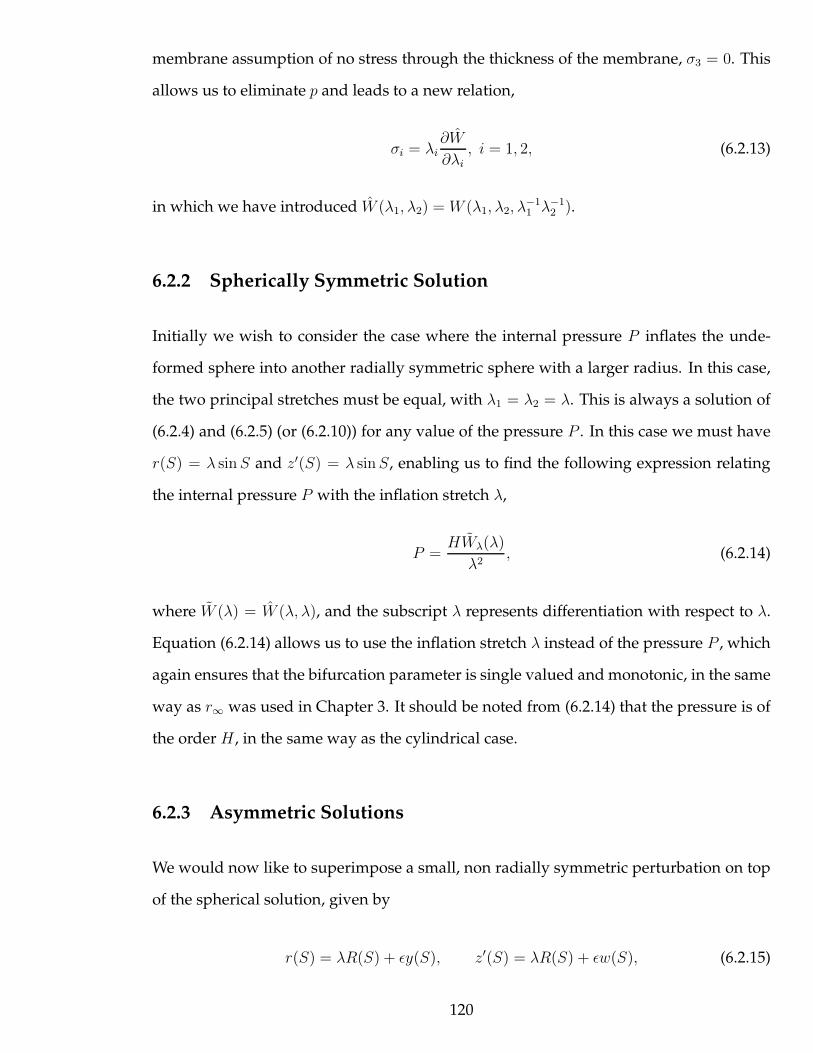
membrane assumption of no stress through the thickness of the membrane, σ3 = 0. This

allows us to eliminate p and leads to a new relation,

σi = λi∂W

∂λi

, i = 1, 2, (6.2.13)

in which we have introduced W (λ1, λ2) = W (λ1, λ2, λ−11 λ−1

2 ).

6.2.2 Spherically Symmetric Solution

Initially we wish to consider the case where the internal pressure P inflates the unde-

formed sphere into another radially symmetric sphere with a larger radius. In this case,

the two principal stretches must be equal, with λ1 = λ2 = λ. This is always a solution of

(6.2.4) and (6.2.5) (or (6.2.10)) for any value of the pressure P . In this case we must have

r(S) = λ sinS and z′(S) = λ sinS, enabling us to find the following expression relating

the internal pressure P with the inflation stretch λ,

P =HWλ(λ)

λ2, (6.2.14)

where W (λ) = W (λ, λ), and the subscript λ represents differentiation with respect to λ.

Equation (6.2.14) allows us to use the inflation stretch λ instead of the pressure P , which

again ensures that the bifurcation parameter is single valued and monotonic, in the same

way as r∞ was used in Chapter 3. It should be noted from (6.2.14) that the pressure is of

the order H , in the same way as the cylindrical case.

6.2.3 Asymmetric Solutions

We would now like to superimpose a small, non radially symmetric perturbation on top

of the spherical solution, given by

r(S) = λR(S) + ǫy(S), z′(S) = λR(S) + ǫw(S), (6.2.15)

120

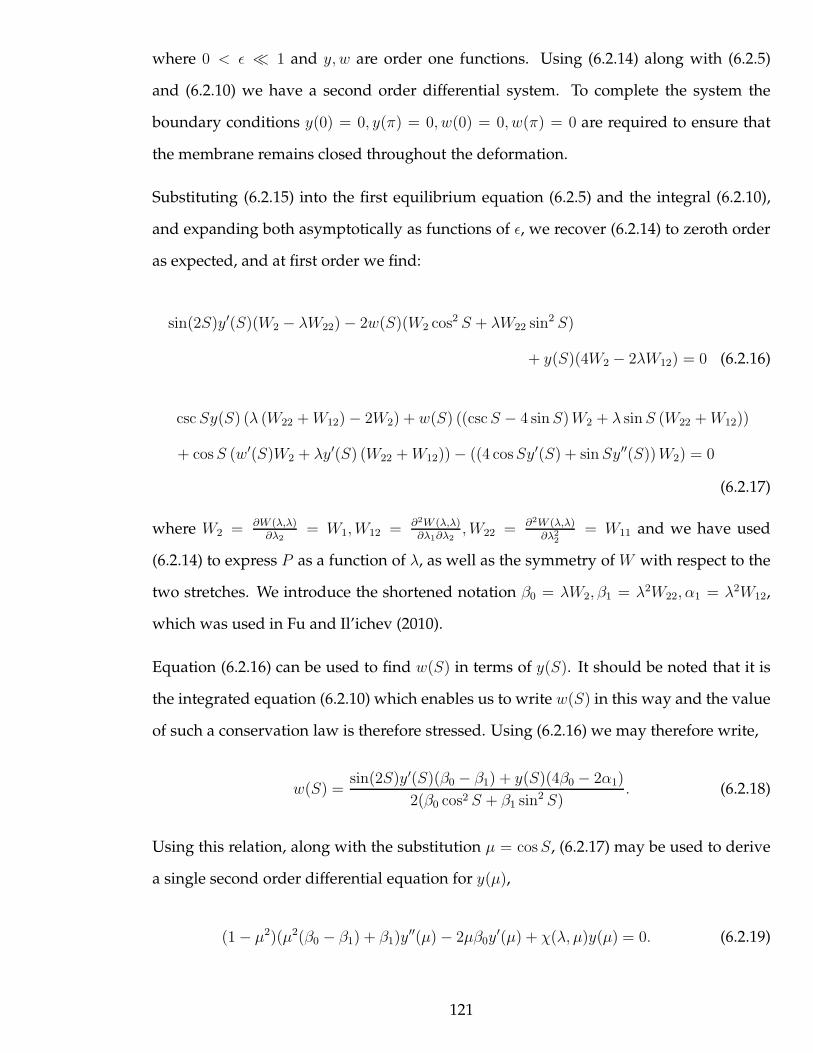
where 0 < ǫ ≪ 1 and y, w are order one functions. Using (6.2.14) along with (6.2.5)

and (6.2.10) we have a second order differential system. To complete the system the

boundary conditions y(0) = 0, y(π) = 0, w(0) = 0, w(π) = 0 are required to ensure that

the membrane remains closed throughout the deformation.

Substituting (6.2.15) into the first equilibrium equation (6.2.5) and the integral (6.2.10),

and expanding both asymptotically as functions of ǫ, we recover (6.2.14) to zeroth order

as expected, and at first order we find:

sin(2S)y′(S)(W2 − λW22) − 2w(S)(W2 cos2 S + λW22 sin2 S)

+ y(S)(4W2 − 2λW12) = 0 (6.2.16)

cscSy(S) (λ (W22 +W12) − 2W2) + w(S) ((cscS − 4 sinS)W2 + λ sinS (W22 +W12))

+ cosS (w′(S)W2 + λy′(S) (W22 +W12)) − ((4 cosSy′(S) + sinSy′′(S))W2) = 0

(6.2.17)

where W2 = ∂W (λ,λ)∂λ2

= W1,W12 = ∂2W (λ,λ)∂λ1∂λ2

,W22 = ∂2W (λ,λ)

∂λ22

= W11 and we have used

(6.2.14) to express P as a function of λ, as well as the symmetry of W with respect to the

two stretches. We introduce the shortened notation β0 = λW2, β1 = λ2W22, α1 = λ2W12,

which was used in Fu and Il’ichev (2010).

Equation (6.2.16) can be used to find w(S) in terms of y(S). It should be noted that it is

the integrated equation (6.2.10) which enables us to write w(S) in this way and the value

of such a conservation law is therefore stressed. Using (6.2.16) we may therefore write,

w(S) =sin(2S)y′(S)(β0 − β1) + y(S)(4β0 − 2α1)

2(β0 cos2 S + β1 sin2 S). (6.2.18)

Using this relation, along with the substitution µ = cosS, (6.2.17) may be used to derive

a single second order differential equation for y(µ),

(1 − µ2)(µ2(β0 − β1) + β1)y′′(µ) − 2µβ0y

′(µ) + χ(λ, µ)y(µ) = 0. (6.2.19)

121

where

χ(λ, µ) =1

β0β1

(

2µ2β30 −

(6 − 8µ2 + µ4)

µ2 − 1β2

0β1 − 2µ2β0β21 + (−1 + µ2)β3

1

− α1β0(3µ2β0 + (5 − 3µ2)β1) + α2

1(µ2β0 − (−1 + µ2)β1)

)

(6.2.20)

Equation (6.2.19) is a linear second order differential equation with variable coefficients,

which is singular at the three points µ = ±1,∞. The boundary conditions become

y(−1) = y(1) = 0, and are to be applied at the singular endpoints of the differential

equation. Writing y(µ) =√

1 − µ2Q(µ), (6.2.19) becomes:

(µ2β0 − (µ2 − 1)β1

)Q′′(µ) − 2µβ1

(

1 − β0(µ2 + 1)

β1(µ2 − 1)

)

Q′(µ) (6.2.21)

−(α1 − 2β0 + β1)(−µ2β20 − 3β0β1 + (µ2 − 1)β2

1 + α1(µ2(β0 − β1) + β1))

(µ2 − 1)β0β1

Q(µ) = 0,

The exact solution to either of the differential equations (6.2.19) and (6.2.21) is not avail-

able in closed form, although it may be solved via series solutions around the singulari-

ties or numerical integration, given a strain-energy function.

6.3 Bifurcation Condition

Haughton and Ogden (1978b) use spherical coordinates throughout their paper, and con-

sider axisymmetric modes in which the stretches in the eρ and eθ directions are expanded

as Legendre polynomials and derivatives of Legendre polynomials. The corresponding

modal perturbation Q(µ) in our notation is Q(µ) = APn(µ) + BµP ′n(µ). Inserting this

ansatz into (6.2.19) and utilising the definition of the Legendre polynomials to simplify

the higher order derivatives as discussed in Section 2.6, we find the following equation:

(AG11(λ, µ) +BG12(λ, µ))Pn(µ) + (AG21(λ, µ) +BG22(λ, µ))P ′n(µ) = 0, (6.3.1)

122

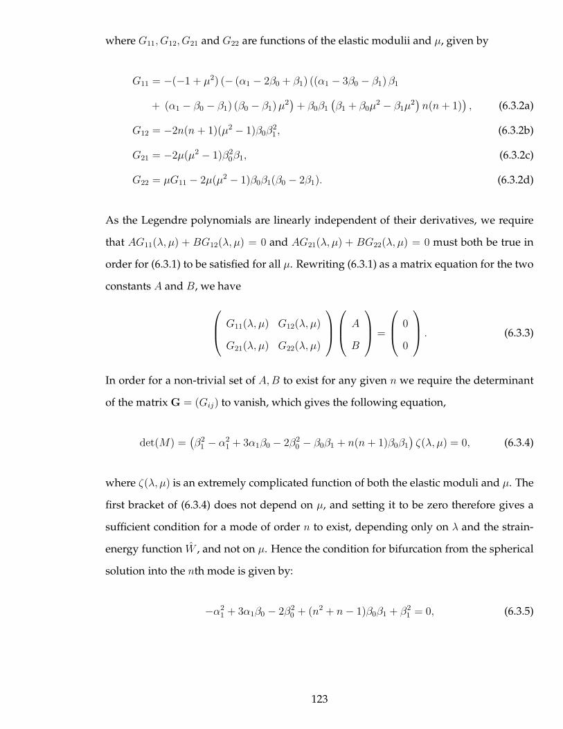
where G11, G12, G21 and G22 are functions of the elastic modulii and µ, given by

G11 = −(−1 + µ2) (− (α1 − 2β0 + β1) ((α1 − 3β0 − β1)β1

+ (α1 − β0 − β1) (β0 − β1)µ2)

+ β0β1

(β1 + β0µ

2 − β1µ2)n(n+ 1)

), (6.3.2a)

G12 = −2n(n + 1)(µ2 − 1)β0β21 , (6.3.2b)

G21 = −2µ(µ2 − 1)β20β1, (6.3.2c)

G22 = µG11 − 2µ(µ2 − 1)β0β1(β0 − 2β1). (6.3.2d)

As the Legendre polynomials are linearly independent of their derivatives, we require

that AG11(λ, µ) + BG12(λ, µ) = 0 and AG21(λ, µ) + BG22(λ, µ) = 0 must both be true in

order for (6.3.1) to be satisfied for all µ. Rewriting (6.3.1) as a matrix equation for the two

constants A and B, we have

G11(λ, µ) G12(λ, µ)

G21(λ, µ) G22(λ, µ)

A

B

=

0

0

. (6.3.3)

In order for a non-trivial set of A,B to exist for any given n we require the determinant

of the matrix G = (Gij) to vanish, which gives the following equation,

det(M) =(β2

1 − α21 + 3α1β0 − 2β2

0 − β0β1 + n(n+ 1)β0β1

)ζ(λ, µ) = 0, (6.3.4)

where ζ(λ, µ) is an extremely complicated function of both the elastic moduli and µ. The

first bracket of (6.3.4) does not depend on µ, and setting it to be zero therefore gives a

sufficient condition for a mode of order n to exist, depending only on λ and the strain-

energy function W , and not on µ. Hence the condition for bifurcation from the spherical

solution into the nth mode is given by:

−α21 + 3α1β0 − 2β2

0 + (n2 + n− 1)β0β1 + β21 = 0, (6.3.5)

123

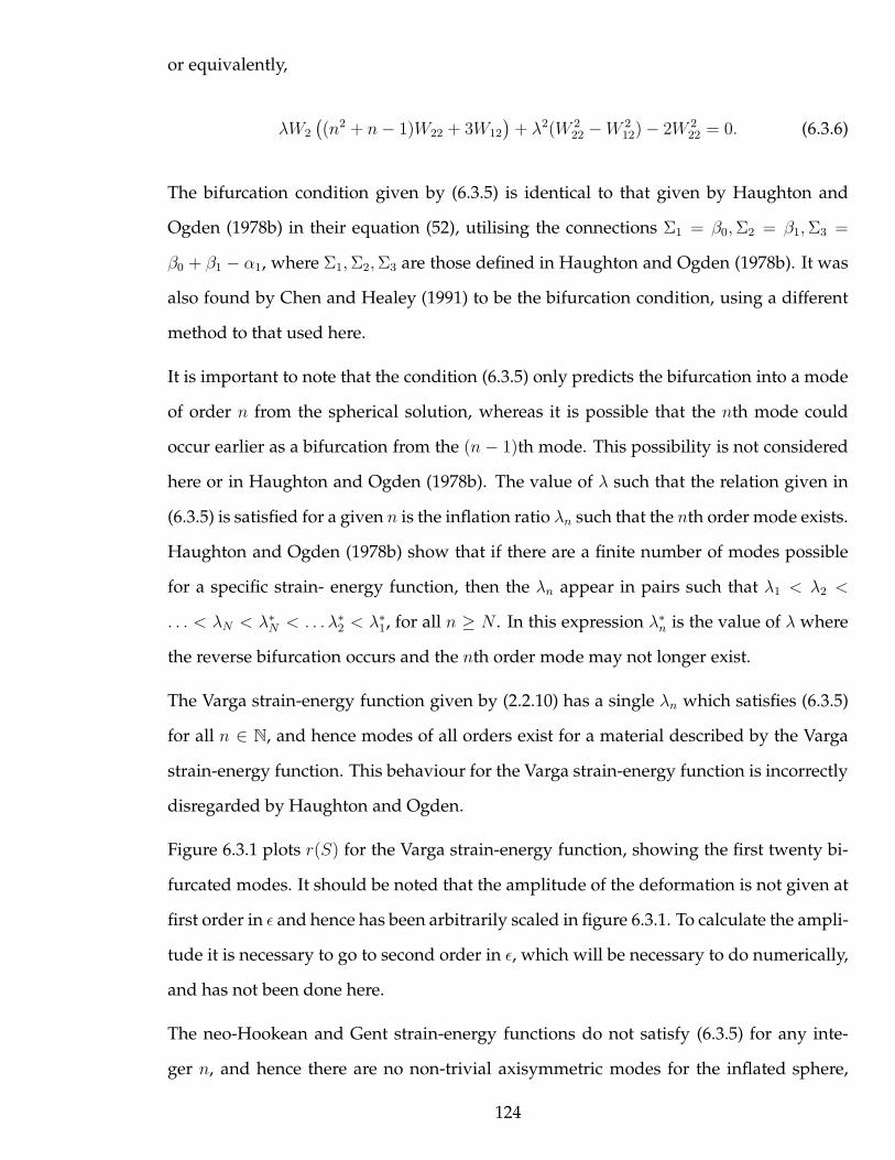
or equivalently,

λW2

((n2 + n− 1)W22 + 3W12

)+ λ2(W 2

22 −W 212) − 2W 2

22 = 0. (6.3.6)

The bifurcation condition given by (6.3.5) is identical to that given by Haughton and

Ogden (1978b) in their equation (52), utilising the connections Σ1 = β0,Σ2 = β1,Σ3 =

β0 + β1 − α1, where Σ1,Σ2,Σ3 are those defined in Haughton and Ogden (1978b). It was

also found by Chen and Healey (1991) to be the bifurcation condition, using a different

method to that used here.

It is important to note that the condition (6.3.5) only predicts the bifurcation into a mode

of order n from the spherical solution, whereas it is possible that the nth mode could

occur earlier as a bifurcation from the (n − 1)th mode. This possibility is not considered

here or in Haughton and Ogden (1978b). The value of λ such that the relation given in

(6.3.5) is satisfied for a given n is the inflation ratio λn such that the nth order mode exists.

Haughton and Ogden (1978b) show that if there are a finite number of modes possible

for a specific strain- energy function, then the λn appear in pairs such that λ1 < λ2 <

. . . < λN < λ∗N < . . . λ∗2 < λ∗1, for all n ≥ N . In this expression λ∗n is the value of λ where

the reverse bifurcation occurs and the nth order mode may not longer exist.

The Varga strain-energy function given by (2.2.10) has a single λn which satisfies (6.3.5)

for all n ∈ N, and hence modes of all orders exist for a material described by the Varga

strain-energy function. This behaviour for the Varga strain-energy function is incorrectly

disregarded by Haughton and Ogden.

Figure 6.3.1 plots r(S) for the Varga strain-energy function, showing the first twenty bi-

furcated modes. It should be noted that the amplitude of the deformation is not given at

first order in ǫ and hence has been arbitrarily scaled in figure 6.3.1. To calculate the ampli-

tude it is necessary to go to second order in ǫ, which will be necessary to do numerically,

and has not been done here.

The neo-Hookean and Gent strain-energy functions do not satisfy (6.3.5) for any inte-

ger n, and hence there are no non-trivial axisymmetric modes for the inflated sphere,

124

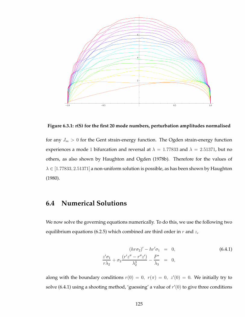
-1.0 -0.5 0.5 1.0

2

4

6

Figure 6.3.1: r(S) for the first 20 mode numbers, perturbation amplitudes normalised

for any Jm > 0 for the Gent strain-energy function. The Ogden strain-energy function

experiences a mode 1 bifurcation and reversal at λ = 1.77833 and λ = 2.51371, but no

others, as also shown by Haughton and Ogden (1978b). Therefore for the values of

λ ∈ [1.77833, 2.51371] a non-uniform solution is possible, as has been shown by Haughton

(1980).

6.4 Numerical Solutions

We now solve the governing equations numerically. To do this, we use the following two

equilibrium equations (6.2.5) which combined are third order in r and z,

(hrσ2)′ − hr′σ1 = 0, (6.4.1)

z′σ1

rλ2+ σ2

(r′z′′ − r′′z′)

λ32

− P ∗

λ3= 0,

along with the boundary conditions r(0) = 0, r(π) = 0, z′(0) = 0. We initially try to

solve (6.4.1) using a shooting method, ‘guessing’ a value of r′(0) to give three conditions

125

at zero, and iterate on the value of r′(0) until the third boundary condition is satisfied.

However, as the equations are singular at the point where we are trying to apply the

boundary conditions, it is difficult to implement a numerical scheme starting at S = 0.

We therefore choose to apply the boundary conditions at a point close to zero, given by

S = δ, where δ ≪ 1. This is viable as the singularity is only an artifact of the cylindrical

coordinate system which we are applying, and is not essential to the problem under

consideration. Expanding the functions around S = 0 we find,

r(δ) = r(0) + r′(0)δ + O(δ2) ≈ r′(0)δ, (6.4.2)

r′(δ) = r′(0) + r′′(0)δ + O(δ2) ≈ r′(0), (6.4.3)

z′(δ) = z′(0) + z′′(0)δ + O(δ2) ≈ z′′(0)δ, (6.4.4)

where we have neglected terms of order δ2 and higher and used the boundary conditions

specified above. We note that r′′(0) = 0 due to the closure requirement at S = 0. Evalu-

ating (6.4.1) as S → 0, we find z′′(0) = P ∗r′(0)3

2W2(r′(0),r′(0)), where we have used the symmetry

of the two arguments of W . Therefore we may now integrate our differential equations

with these boundary conditions, using the shooting method described previously, with

just r′(0) as the only parameter to shoot on. Figure 6.4.1 shows an example of the calcu-

lated profile of r(S) for the Varga strain-energy function after the mode one bifurcation,

while Figure 6.4.2 shows the mode two bifurcation. In Figure 6.4.1, the value of λ at that

point is equal to λ1, where the onset of the mode one bifurcation occurs. This means that

the post-bifurcation path must have turning points the curve must track back on itself,

as at the bifurcation point itself the non-uniform solution must not exist. Similarly with

Figure 6.4.2, which is at λ = 1.8874 < λ3 = 1.9767.

126

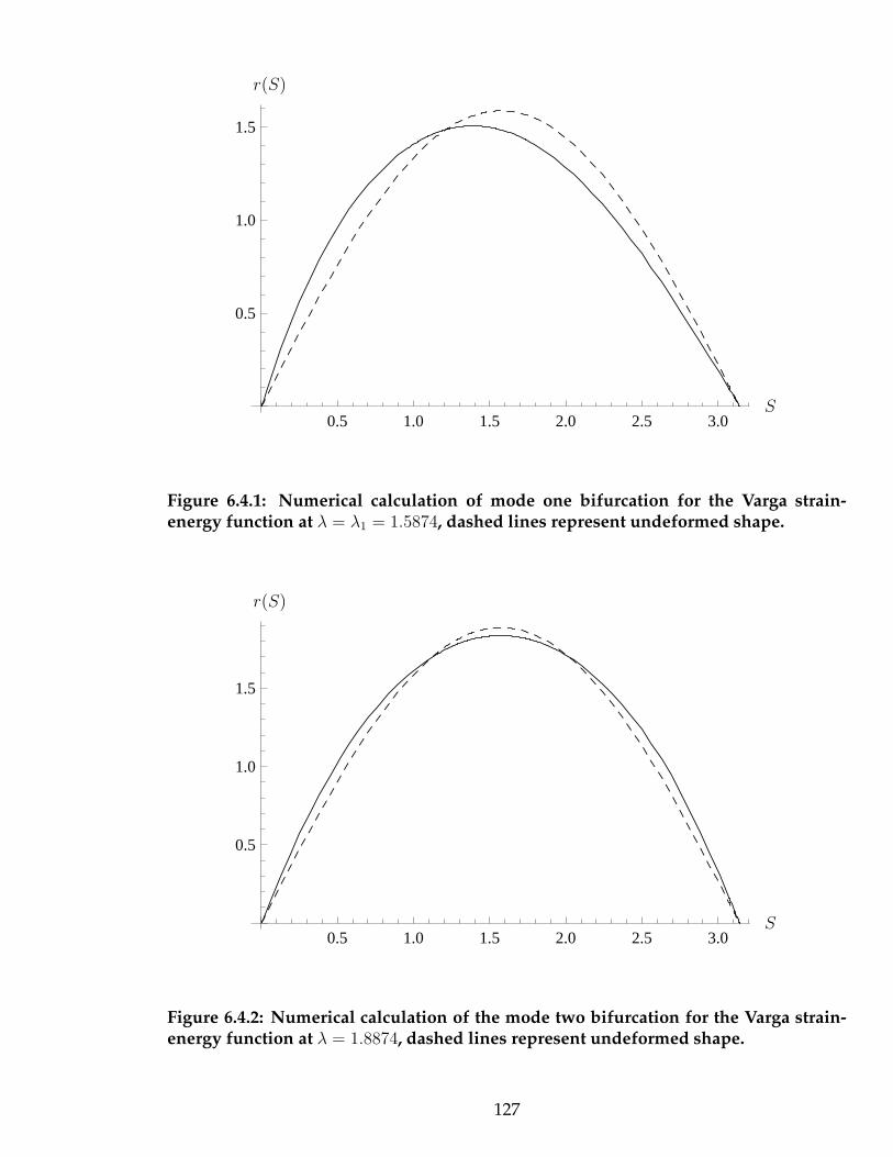
0.5 1.0 1.5 2.0 2.5 3.0

0.5

1.0

1.5

S

r(S)

Figure 6.4.1: Numerical calculation of mode one bifurcation for the Varga strain-energy function at λ = λ1 = 1.5874, dashed lines represent undeformed shape.

0.5 1.0 1.5 2.0 2.5 3.0

0.5

1.0

1.5

S

r(S)

Figure 6.4.2: Numerical calculation of the mode two bifurcation for the Varga strain-energy function at λ = 1.8874, dashed lines represent undeformed shape.

127

6.5 Biological Cells

Skalak et al. (1973) consider the deformation of red blood cells which have been ’sphered’

by the addition of a hypotonic solution, so that they change from their natural, dumb-

bell shape to a sphere. They report the results of experimental testing on red blood cells,

which give (linear) elastic modulii ranging from 7.2 ∗ 105 − 3.0 ∗ 108dyn/cm2 in different

methods of testing. Skalak et al. conclude that the reason behind the wide variation in

measured values is that the membrane has a high intrinsic resistance to deformations

which change the surface area of the cell, and hence nonlinear elasticity is required to

model the membrane accurately. This area-conserving property has been used as a for-

mal constraint on the elastic deformations by later authors, such as Liu et al. (2006).

Skalak et al. (1973) introduce a two-dimensional membrane strain-energy function, where

the theory does not explicitly involve the thickness, given by

W =B

4(1

2K2

1 +K1 −K2) +C

8K2

2 , (6.5.1)

where B,C are constants, K1 = λ1+λ2−2 is an invariant measuring the shearing compo-

nent and K2 = λ21λ

22 − 1 is an invariant which becomes zero when the areal strain is zero,

regardless of the magnitude of the stretches. Skalak et al. (1973) suggest that constant

C is at least three orders of magnitude larger than B in (6.5.1) in order to qualitatively

model experimental data with the high resistance to area altering deformations.

6.5.1 Constant Area Constraint

If we impose this area conservation of cells as a constraint on the material properties in

the sense of finite elasticity in addition to the standard incompressibility constraint, we

require that

λ1λ2 = 1, λ3 = 1. (6.5.2)

128

The addition of this second constraint requires us to introduce another Lagrange multi-

plier as well as the one associated with incompressibility. Starting with the second equi-

librium equation (6.2.5) and the conservation law (6.2.10), we introduce the constrained

stresses appropriately as

σi = λi∂W (λ1, λ2)

∂λi− q, i = 1, 2 (6.5.3)

where q is the Lagrange multiplier associated with the constrained area and we set λ1λ2 =

1 after differentiating.

We now perform the same analysis as for the proceeding case, looking for deformed

configurations which are not radially symmetric. It is clear that the spherical expansion

state which is found in the unconstrained case can not exist except for λ = λ1 = λ2 =

1, so we expand from the undeformed configuration instead of the spherically inflated

configuration. Substituting (6.5.3) into (6.2.5) and (6.2.10) and using (6.5.2), we find

2rH(W2 − q)z′

λ1λ22

− P ∗r2 = 0, (6.5.4)

z′(W1 − q)

rλ2

+ (W2 − q)(r′z′′ − r′′z′)

λ32

− P ∗ = 0, (6.5.5)

where Wi = ∂W∂λi

|λ2=λ−11

After eliminating λ2 and λ3 by using (6.5.2), equation (6.5.4) can be rearranged to find q

is given by,

q =λ3

1P∗r

2z′− λ1W1. (6.5.6)

Hence, (6.5.5) becomes, using (6.5.6),

−λ21P

∗ +2z′

r(W1 −W2) + P ∗r

(

−r′′ + r′z′′

z′

)

= 0. (6.5.7)

Expanding r and z′ around the undeformed state in the same manner as for the uncon-

strained case, but with λ = 1, r(S) = sinS + ǫy(S), z′(S) = sinS + ǫw(S), we find (6.5.7)

129

becomes at first order in ǫ,

(−1 + 4γ) cscSy(S) + cosS (− cotSw(S) + w′(S) + y′(S)) − sinSy′′(S) = 0, (6.5.8)

where γ = 2G/P ∗ and 2G = W11(1, 1) −W12(1, 1) is the shear modulus of the material.

We note that in this case, in contrast to the unconstrained case considered in the previous

section, there is no equation which determines P at the zeroth order which would be a

counterpart of (6.2.14).

The second differential equation which we require can be derived from considering the

first order in ǫ of λ2 =√r′2 + z′2 = λ−1

1 and is given by

sinSw(S) + cscSy(S) + cosSy′(S) = 0, (6.5.9)

which may be solved for w(S). Substituting (6.5.9) into (6.5.8) we find a single differential

equation for y(S), given by

(−(1 + 2γ) + 2(γ − 1) cos(2S)) y(S) + sinS(− cosSy′(S) + sinSy′′(S)) = 0. (6.5.10)

Using the transformation µ = cosS the differential equation can be written as an associ-

ated Legendre function in the following way,

(1 − µ2)Y ′′(µ) − 2µY ′(µ) +

(

4γ − 4µ2

1 − µ2

)

Y (µ) = 0, (6.5.11)

where Y (µ) = sinSy(cosS), and the relation of (6.5.11) to the associated Legendre equa-

tion is given by l(l + 1) = 4γ,m2 = 4. Therefore the solutions of (6.5.11) are given by

y(S) = A sinSP 212(−1+

√17+16γ)

(cosS) +B sinSQ212(−1+

√17+16γ)

(cosS). (6.5.12)

The required boundary conditions for closure of the membrane are y(0) = y(π) = 0.

The first of these is always satisfied by (6.5.12) provided B = 0, for any γ. In order

to satisfy the second boundary condition we have the solvability condition that 12(−1 +

130

√17 + 16γ) = k, where k ∈ Z, to reduce the solution to a Legendre polynomial, else the

solution is infinite at S = π. Rearranging this equation for γ we find

γ =1

4(k2 + k − 4), k ∈ Z. (6.5.13)

However, using the definition of γ, we can rewrite (6.5.13) for P ,

P =−4HG

k2 + k − 4. (6.5.14)

In the derivation of the governing equations it is a requirement that the pressure P is

positive to ensure that the membrane is in tension and not compression. When one of

the principal stresses becomes negative then the membrane will form wrinkles as dis-

cussed in Section 2.3.4, and a relaxed strain-energy function is required to describe this

occurrence satisfactorily (Pipkin 1986). Hence, as the shear modulus and the thickness

H are all positive, we require that the integer k satisfies k2 + k − 4 < 0 to give a positive

pressure from (6.5.14). This is only satisfied if k = −2,−1, 0, 1. So admissible solutions of

the differential equation are given by

y(S) = A sinSP 2k (cosS), (6.5.15)

where k = −2,−1, 0, 1. However, from the properties of the Legendre polynomials

Pmn (x), if −(m + 1) < n < m then the polynomial is everywhere zero. Therefore we

conclude that there can be no non-trivial solutions to the inflation of an incompressible

spherical membrane when the area is rigidly constrained in this manner.

6.6 Conclusion

In this chapter we have rederived the bifurcation condition given in Haughton and Og-

den (1979a) and Chen and Healey (1991), utilising the integral arising from the conserva-

tion law.

131

When n = 0, the bifurcation condition (6.3.5) becomes dPdλ

= 0, and this must occur

before the n = 1 mode, as discussed in Haughton and Ogden (1979a). In Chapter 3

the bifurcation condition which was found for the cylindrical tube corresponded to the

zeroth mode in the linear bifurcation analysis, leading to a weakly nonlinear bifurcation

analysis. This leads us to speculate that there may be a similar localised solution in the

spherical case considered here, although we have not investigated this possibility and it

remains as future work.

With respect to the constraint of area preservation on the surface of the membrane, we

found that if the constraint is rigidly applied then no non-trivial solutions may exist.

However, if the inflation of a shell was considered, the inclusion of the bending moments

may allow the existence of non-trivial solutions, but this has not been considered here.

132

Chapter 7

Inflation of a General Axisymmetric

Shell

7.1 Introduction

In this chapter we consider the axisymmetric inflation of a thin axishell via an internal

pressure, rather than the cylindrical and spherical membranes considered in the previ-

ous chapters. Referring back to the definitions introduced in Section 2.3, we recall that an

axishell is a thin axisymmetric shell whose response to deformation includes a contribu-

tion from bending in addition to the stretching response found in membranes. Initially

we specialise the governing equations for a static deformation of a two-dimensional elas-

tic surface deformed via an internal pressure, including the bending moments. We follow

this by showing that, for an arbitrary axishell, a conservation law integral exists gener-

alising the first such integral found in Chapter 3 for the cylindrical membrane and in

Chapter 6 for the spherical membrane. After this we compare with the governing equa-

tions given in Chapter 6 for the spherical membrane, and the literature on the inflation

of initially spherical axishells, showing that the governing equations derived here for the

two-dimensional theory are identical with those for the three-dimensional theory, with

an appropriate change in the definition of the strain-energy function. We conclude with

133

a discussion of biological fluid-like lipid bilayers, which are commonly modelled in the

literature as elastic surfaces which only have contributions to the energy from bending,

not stretching.

We shall use the theory of Steigmann and Ogden (1999) to describe the deformation of an

axisymmetric two-dimensional elastic surface embedded into three-dimensional space,

subject to axisymmetric deformations. In particular, we allow the energy of the material

to depend on both the stretching of the elastic elements and the curvatures develop-

ing within the shell. This is an extension of the theories discussed previously, and is a

thin-shell theory as opposed to a membrane theory. In addition, it extends the theory

of nonlinear elasticity from Cauchy elasticity as the response of the material no longer

depends only on the value of the deformation gradient F, but also on the curvatures in

the deformed configuration. These curvature terms are functions of the gradient of the

deformation gradient, ∇F, but the energy is not allowed to depend generally on ∇F.

The notation and derivations here correspond to those used in Steigmann and Ogden

(1999), who present a theory of elastic surface-substrate interactions wherein they con-

sider the deformation of a thin coat of substrate bonded to a material, which may have

different material properties. We shall use this theory without the solid body, to just de-

scribe the deformation of the thin elastic sheet. A variational treatment of this derivation

may be seen in Baesu et al. (2004), although we work directly from Steigmann and Ogden

(1999). We also note that Steigmann (2001) reiterates much of this theory, with additional

details and explanations.

7.2 Deformation of Axisymmetric Shells

7.2.1 Derivation

We consider a position function Y on the shell which is parameterised locally by two

coordinates θα, where α and all future Greek sub- and superscripts take the values 1 or 2.

134

Thus Y is the two-dimensional equivalent of X in Chapter 2. In the same way as noted

in Chapter 2, capital and small letters shall be used to denote the same quantities in the

reference and current configurations respectively wherever possible.

We define the reference configuration with respect to cylindrical coordinates, (R,Θ, Z),

and it is parameterised by

θ1 = AΘ, θ2 = S, (7.2.1)

where Θ is the angle around the axis of symmetry, S is the arc length around the sphere

andA is a lengthscale. The basis of three dimensional space which we will use is (er, eθ, ez)

as unit vectors in the R, Θ and Z directions respectively. We remain in cylindrical coordi-

nates for convenience due to the axisymmetry, and choose to use the same basis for both

the reference and current configurations. Therefore Y is given by,

Y(θ1, θ2) = R(S)er(Θ) + Z(S)ez. (7.2.2)

The two reference configurations which we are particularly interested in here are the

cylindrical case, corresponding to the case considered in Chapter 3, and the spherical

case. For the cylindrical case,

R(S) = A, Z(S) = S, (7.2.3)

whereas for the spherical case,

R(S) = A sin(S/A), Z(S) = A(1 − cos(S/A)), (7.2.4)

where we have chosen to define the coordinate system such that Z ′(S) is positive.

The shell deforms to a current configuration y described by cylindrical coordinates, (r,Θ, z),

where we have imposed the condition of axisymmetry. Therefore y is given by,

y(θ1, θ2) = r(S)er(Θ) + z(S)ez. (7.2.5)

135

These coordinates induce tangent vectors to the surface of the shell in the reference con-

figuration,

Gα = Y,α, gα = y,α, (7.2.6)

where ,α represents differentiation with respect to θα, and therefore ,1 = 1A

∂∂Θ,,2 = ∂

∂S. The

tangent vectors in the reference configuration are then given by,

G1 = Y,1 =R(S)

Aeθ, G2 = Y,2 = R′(S)er + Z ′(S)ez, (7.2.7)

where hereon a prime represents differentiation with respect to S. We find the compo-

nents of the metric tensors (Gαβ), (Gαβ) as well as the dual vectors Gα, using the follow-

ing formulae, Gαβ = Gα.Gβ, Gα.Gβ = δαβ , Gαβ = Gα.Gβ, as

G11 =R2

A2, G12 = G21 = 0, G22 = R′2 + Z ′2, (7.2.8)

G11 =A2

R2, G12 = G21 = 0, G22 =

1

(R′2 + Z ′2), (7.2.9)

G1 =A

Reθ, G2 =

R′

√R′2 + Z ′2

er +Z ′

√R′2 + Z ′2

ez, (7.2.10)

G = det(Gαβ) =R2(R′2 + Z ′2)

A2, (7.2.11)

and thus the normal in the reference configuration is given by

N =1√G

(G1 ∧ G2) =A

R√R′2 + Z ′2

(RZ ′

Aer −

RR′

Aez)

=Z ′er − R′ez√R′2 + Z ′2

. (7.2.12)

The derivatives of the tangent vectors (7.2.7) are given by

G1,1 = − R

A2er, G1,2 = G2,1 =

R′

Aeθ, G2,2 = −R′′er + Z ′′ez. (7.2.13)

The reference normal curvatures associated with the embedding of the surface into the

136

three-dimensional space, Bαβ = N · Gα,β, are given by

B11 = − RZ ′

A2√R′2 + Z ′2

, B12 = B21 = 0, B22 =(R′′Z ′ −R′Z ′′)√

R′2 + Z ′2, (7.2.14)

Similarly, in the deformed configuration we may define all the equivalent quantities,

starting with the tangent vectors,

g1 = y,1 =r(S)

Aeθ, g2 = y,2 = r′(S)er + z′(S)ez, (7.2.15)

We find the components of the metric tensors (gαβ), (gαβ) as well as the dual vectors gα,

all defined in the same way as for the undeformed configuration, as

g11 =r2

A2, g12 = g21 = 0, g22 = (r′2 + z′2), (7.2.16)

g11 =A2

r2, g12 = g21 = 0, g22 =

1

(r′2 + z′2), (7.2.17)

g1 =A

reθ, g2 =

r′er + z′ez

(r′2 + z′2), (7.2.18)

g = det(gαβ) =r2(r′2 + z′2)

A2, J = g/G, (7.2.19)

and thus the normal in the current configuration is,

n =1√g(g1 ∧ g2) =

1

r√r′2 + z′2

(rz′

Aer −

rr′

Aez),

=z′er − r′ez√r′2 + z′2

. (7.2.20)

The derivatives of the tangent vectors are given by

g1,1 = − r

A2er, g1,2 = g2,1 =

r′

Aeθ, g2,2 = r′′er + z′′ez. (7.2.21)

And the components of the embedded deformed curvature tensor are then given using

bαβ = n · gα,β,

b11 = − rz′

A2√r′2 + z′2

, b12 = b21 = 0, b22 =(r′′z′ − r′z′′)√

r′2 + z′2. (7.2.22)

137

The Christoffel symbols on the deformed surface are given by Γγαβ = gγ.gα,β and become,

Γ111 = 0, Γ2

11 =−rr′

A(r′2 + z′2), (7.2.23)

Γ112 =

r′

r, Γ2

12 = 0, (7.2.24)

Γ121 =

r′

r, Γ2

21 = 0, (7.2.25)

Γ122 = 0, Γ2

22 =r′r′′ + z′z′′

r′2 + z′2. (7.2.26)

Using the chain rule we may write,

gα = FGα, (7.2.27)

where F is the surface deformation gradient, F = gβ⊗Gβ . Therefore we have the Cauchy

Green surface deformation tensor C, given by

C = FT F = gαβGα ⊗ Gβ. (7.2.28)

The relative curvature κ = −b, given with respect to the undeformed dual metric tensors

is,

κ = καβGα ⊗ Gβ. (7.2.29)

7.3 Equilibrium Equations

We define y as an incremental variation in y, and henceforth a superimposed dot denotes

an incremental variation in the relevant quantity. Assuming that the energy of the sur-

face is given by a strain-energy function U , which is a function of both the deformation

gradient C, and the curvature κ, Steigmann and Ogden (1999) show that

U = Tα · y,α + Mαβ · y,αβ , (7.3.1)

138

where

Tα ≡ J(σαβgβ +mλβΓαλβn), Mαβ ≡ −Jmαβ , (7.3.2)

Jσαβ =∂U

∂gαβ+

∂U

∂gβα, Jmαβ =

∂U

∂καβ. (7.3.3)

In (7.3.2), σαβ and mαβ are the contravariant components of the stress and moment ten-

sors in the deformed configuration respectively. These components may be related to the

covariant components which are generally used by, σαβ = gαβσαβ and a similar formula

holds for the moments (Epstein and Johnston 2001).

Steigmann and Ogden (1999) then derive how the increment of the energy of the static

elastic surface may be written as,

∮

P

UdA =

∮

P

G−1/2[(G1/2Tα),α − (G1/2Mβα),βα],α · ydA, (7.3.4)

where a superimposed dot represents the increment. This leads to the following equilib-

rium equation,

G−1/2[(G1/2Tα),α − (G1/2Mβα),βα] = ST N, (7.3.5)

where S is the three-dimensional nominal stress tensor associated with the forces acting

on the elastic surface as defined in (2.1.42). We note the connections between these three-

dimensional , ST = JσF−T , and N = FT n.

This enables us to write the external forces from (7.3.5) as,

STN = JσF−TFT n = Jσn. (7.3.6)

If the external forces are given by a constant hydrostatic pressure P in the deformed

configuration, then σn = −Pn, and therefore using J =√g/√G we have,

STN = −JP z′er√r′2 + z′2

+ JPr′ez√r′2 + z′2

= −P rz′√G

er + Prr′√G

ez. (7.3.7)

139

7.3.1 Evaluating the Equilibrium Equations

We now non-dimensionalise with respect to A, which we do implicitly by setting A = 1

and considering all lengths, including S, to be rescaled with respect to A. Evaluating the

equilibrium equation (7.3.5) gives,

(Jσ22r′√G)′√

G− Jσ11 r

A− 1√

G

(

Jm11rr′z′√G

A(r′2 + z′2)3/2

)′

− Jm11z′

(r′2 + z′2)1/2+

1√G

(

(Jm22z′√G)′

(r′2 + z′2)1/2

)′

+ Prz′√G

= 0,

(7.3.8)

in the er direction, and

(Jσ22z′√G)′√

G+

1√G

(

Jm11rr′2√G

A(r′2 + z′2)3/2

)′

− 1√G

(

(Jm22r′√G)′

(r′2 + z′2)1/2

)′

− Prr′√G

= 0, (7.3.9)

in the ez direction, where we recall that√G = R(R′2 + Z ′2)1/2/A.

We now note that, after multiplying through by√G, (7.3.9) may now be integrated to

give the resultant in the Z-direction as,

Jσ22z′R√R′2 + Z ′2−Jm11rr′2R

√R′2 + Z ′2

(r′2 + z′2)3/2+

(Jm22r′R√R′2 + Z ′2)′

(r′2 + z′2)1/2−P ∗r2

2= C1, (7.3.10)

where C1 is a constant of integration which will be determined by the boundary con-

ditions of the case under consideration. The exploitation of this integral allowed us to

derive the bifurcation conditions in the cylindrical and spherical cases in Chapters 3 and

6 respectively.

It is possible to combine these equations to give expressions in the directions normal and

tangent to the deformed surface, that is n and (r′er + z′ez)/√r′2 + z′2 respectively. In the

140

tangential direction, we find

√r′2 + z′2

(

σ22

√G√

r′2 + z′2

)′

− σ11

√Gr′

r− m11r

′z′√G

r2√r′2 + z′2

+m11r

′√G

r(r′2 + z′2)3/2(z′r′′ − r′z′′)

+√r′2 + z′2

(

m22

√G(z′′r′ − r′′z′)

(r′2 + z′2)2

)′

+

(

m22

√G√

r′2 + z′2

)′(z′′r′ − r′′z′)

(r′2 + z′2)= 0.

(7.3.11)

We note that it is possible to combine the last two terms in (7.3.11) by using either of the

two following identities, (xy)′ + x′y = 2x′y + xy′ = (x2y)′/x = 2√y(x

√y)′, although they

are not immediately useful here. In the normal direction, we find

(z′r′′ − r′z′′)

(

σ22

√G

(r′2 + z′2)

)

− σ11

√Gz′

r− m11z

′2√G

r2√r′2 + z′2

−√r′2 + z′2

(

m11r′√G

(r′2 + z′2)

)′

+z′

(

1√r′2 + z′2

(

m22z′√G

(r′2 + z′2)

)′)′

+ r′

(

1√r′2 + z′2

(

m22r′√G

(r′2 + z′2)

)′)′

+ P ∗r(r′2 + z′2) = 0

(7.3.12)

7.4 Invariants

The axisymmetric configurations which are under consideration here are necessarily

hemitropic, and the energy must be invariant with respect to rotations around the axis of

symmetry. Therefore we use equation (6.20) from Steigmann and Ogden (1999) to find

the invariants of the deformation,

I1 = trC = gαβGαβ =

r2

R2+

(r′2 + z′2)

R′2 + Z ′2, (7.4.1a)

I2 = detC =g

G=

r2(r′2 + z′2)

R2(R′2 + Z ′2), (7.4.1b)

I3 = trκ = καβGαβ =

rz′

R2√r′2 + z′2

+(r′z′′ − r′′z′)√

r′2 + z′2(R′2 + Z ′2), (7.4.1c)

I4 = detκ =1

Gκ11κ22 =

rz′(r′z′′ − r′′z′)

R2(r′2 + z′2)(R′2 + Z ′2), (7.4.1d)

with another three invariants corresponding to coupling terms between the stresses and

bending moments which are not considered here. From (7.4.1a) and (7.4.1b), we may see

141

that the principal stretches may be written as,

λ1 =r2

R2, λ2 =

√r′2 + z′2√R′2 + Z ′2

, (7.4.2)

corresponding with those used in the preceding chapters, although without the third

stretch as the formulation here is two-dimensional. The stresses and moments are given

by Steigmann and Ogden (1999),

1

2Jσαβ =

∂U

∂I1Gαβ +

∂U

∂I2Cαβ (7.4.3)

Jmαβ = 2I3∂U

∂I23

Gαβ +∂U

∂I4καβ, (7.4.4)

where a tilde represents the adjugate of a tensor from T = (trT)I − T, although care

must be taken to use the correct trace of the tensor, i.e. I1 or I3 for C or κ respectively,

rather than just the sum of the two components. We may also use the formulae, Cαβ =

I2gαβ, καβ = µαγµβλκγλ, where µαβ = eαβ/

√G, where eαβ is the alternator symbol with

e11 = e22 = 0, e12 = 1, e21 = −1.

C11 =r′2 + z′2

R2(R′2 + Z ′2), C22 =

r2

R2(R′2 + Z ′2), (7.4.5)

κ11 =κ22

A2R2(R′2 + Z ′2), κ22 =

κ11

A2R2(R′2 + Z ′2). (7.4.6)

7.4.1 Membrane Theory

As discussed previously in Section 2.3, the membrane theory ignores the contribution

to the energy from the curvature of the surface. Therefore, for a membrane we assume

that U is a function of I1 and I2 only, and therefore m11 = m22 = 0. Using the covariant-

contravariant connections, σ11 = r2σ11, σ22 = (r′2 + z′2)σ22, we find (7.3.8) and (7.3.9)

142

become,

(

Jσ22

√Gr′

λ22

)′

− Jσ11

√G

r+ P ∗rz′ = 0, (7.4.7)

(

Jσ22

√Gz′

λ22

)′

− P ∗rr′ = 0, (7.4.8)

In the cylindrical case,√G = 1 as given in (7.2.3), we may immediately see (7.4.7) and

(7.4.8) can be reduced to be the static form of the equations of motion in Chapter 3 (3.3.13),

after using the connections Jσ11 = σ1, Jσ22 = σ2. This is therefore the connection between

the two dimensional theory developed here, and the three dimensional theory used in

Chapter 3. The two integrals used in Chapter 3 still exist here, with the first of them

corresponding to (7.3.10).

For the spherical case, using (7.2.4), we find that (7.4.7) and (7.4.8) are equivalent to the

equilibrium equations given in Chapter 6, (6.2.4) and (6.2.5). To see this, the equations

(7.3.11) and (7.3.12), which are given in tangential and normal directions respectively,

may be used. Again we require the connections Jσ11 = σ1, Jσ22 = σ2 between the two-

and three- dimensional theories.

7.5 Specialisation

7.5.1 Shell Theory

In the literature on deformations of spherical shells, the following three differential equa-

tions are introduced, such as by Pamplona and Calladine (1993), Pozrikidis (2001), Blyth

and Pozrikidis (2004), Liu et al. (2006), Preston et al. (2008):

d(rN2)

ds−N1

dr

ds−Qrκ2 = 0, (7.5.1a)

N1κ1 +N2κ2 +1

r

d(Qr)

ds= P, (7.5.1b)

d(rM2)

ds−M1

dr

ds+Qr = 0, (7.5.1c)

143

where s is the arc length in the deformed configuration, N1, N2,M1,M2 are principal

stress resultants and bending moments respectively, Q is the transverse shear tension

and the principal curvatures are given by,

κ1 =κ11

r2, κ2 =

κ22

(r′2 + z′2). (7.5.2)

Equation (7.5.1a) and (7.5.1b) are in the tangential and normal directions respectively. In

order to compare with our derived equations, we need the connections,

Ni = hσii =R

r√r′2 + z′2

σii, Mi = hmii =R

r√r′2 + z′2

mii, (7.5.3)

and the formula dsdS

=√r′2 + z′2 as was discussed in Chapter 6. Using these formulae we

may convert (7.3.11) and (7.3.12) into three equations as in (7.5.1), which are given by,

d(rN2)

ds−N1

dr

ds−Qrκ2 −

M1

r

dr

ds

dz

ds+d(M2rκ2)

ds︸ ︷︷ ︸

= 0, (7.5.4a)

N1κ1 +N2κ2 +1

r

d(Qr)

ds+

1

r2M1

dz

ds

2

+ κ22M2

︸ ︷︷ ︸

= P, (7.5.4b)

d(rM2)

ds−M1

dr

ds+Qr = 0. (7.5.4c)

In (7.5.4) there are additional terms to those in (7.5.1), indicated by the underbraces.

These terms only involve the bending moments, and therefore when the membrane the-

ory is considered the two derivations are equivalent. We also remark that it does not

seem possible to include the additional terms in the definition of Q, given by (7.5.4c),

and retain the structure of the remaining equations. The equations in (7.5.1) only contain

an integral when the membrane assumption is made, M1 = M2 = 0. This discrepancy

requires further investigation, although it shall be left as future work here. In particular,

the existence of the integral (7.3.10) would reduce the system of equations by one.

144

7.5.2 Biological Lipid Bilayers

Many biological membranes consist of lipid bilayers, where a double layer of long, rela-

tively rigid molecules is orientated normal to the surface (Jenkins 1977). These molecules

have hydrophilic heads and hydrophobic tails, and therefore molecular forces keep the

membranes intact (McMahon and Gallop 2005). Such bilayers have fluid-like properties,

and have often been modelled as continua which have negligible resistance to stretching

but do resist changes to their curvature.

In order to model such lipid bilayers, Zhong-Can and Helfrich (1989) and Jian-Guo and

Zhong-Can (1993) introduce a variational formulation in which they minimise the varia-

tions of the following integral,

E = kc

∮

(κφ + κs − c0)2dA+ ∆p

∫

dV, (7.5.5)

where kc is the bending rigidity, c0 is the spontaneous curvature in the undeformed state,

and ∆p is the pressure difference across the surface. The connection between the curva-

tures in (7.5.5) and those defined previously is given by,

κφ =κ11

r2, κs =

κ22

A2(r′2 + z′2), (7.5.6)

where it should be noted that r2 = g11 and A2(r′2 + z′2) = g22, so κ11g11 = κφ, κ22g

22 = κs.

Blyth and Pozrikidis (2004) review the literature on this variational formulation, and

state a differential equation in terms of the curvature ks which was found by Jian-Guo

and Zhong-Can (1993). They discuss how several further authors have shown an inte-

gral of this equation exists, but there appears to be confusion in the literature as to the

correct behaviour in certain limits. Blyth and Pozrikidis (2004) also discuss the alterna-

tive shell theory approach, but do not manage to make any connections between the two

approaches.

We may therefore connect the integrand in (7.5.5) with our derivations above by noting

that it may be written as (κ11λ21+κ22λ

22−c0)2, which is precisely the third invariant (I3−c0)2

145

as would be expected. We should therefore be able to compare the two approaches, in

particular we would like to see how the integral given in (7.3.10) relates to that which

was discussed in Blyth and Pozrikidis (2004), but we leave this as future work.

7.6 Conclusions and Future Work

In this chapter we have derived the equations for an axisymmetric shell which is sub-

jected to a constant transmural pressure using two-dimensional elasticity, and compared

with those used in the preceding chapters for membranes which were found using three-

dimensional elasticity. We have shown an integral exists for a general axisymmetric shell

and encourage its use whenever possible in order to reduce the order of the differen-

tial equations by one. We have found discrepancies between the equilibrium equations

(7.3.8) - (7.3.9) and those given by Preston et al. (2008) and others. The equations given

in Preston et al. (2008) are derived via force and moment balances, and it is possible that

components have been overlooked in this derivation. The two approaches agree when

the strain-energy only depends on the stretches, not the curvatures. Resolving this dis-

crepancy has been left as future work which should be undertaken.

The modelling of biological lipid bilayers was briefly discussed and the connection be-

tween the theory given here and that discussed in Jian-Guo and Zhong-Can (1993) and

others was shown, although this is also left as future work. In particular, the connection

between the shell theory equations given by (7.3.8) - (7.3.9) with the equation resulting

from the calculus of variations appearing in Jian-Guo and Zhong-Can (1993) should be

investigated.

146

Chapter 8

Optical Tweezers

8.1 Introduction

The deformation of biological cells placed into a fluid flow is important in clinical medicine

and the biological sciences. Cells which are inserted into the blood stream in one location

may be deformed due to the stresses from the fluid flow before arriving at their intended

destination. Such deformation could have major effects on the function of the cells, such

as regulating the gene expressions of the cell. McCormick et al. (2001) show that many

of the genes in endothelial cells are regulated by shear stresses, altering the expressed

phenotypes, as also discussed in Frangos et al. (1988) and Bao and Suresh (2003). We are

particularly interested here in stem cells, which are pluripotent cells with the potential to

differentiate into various other types of cell (Deans and Moseley 2000). They are therefore

considered useful in stem cell therapy treatments, where cells are inserted into the body

as described above. Hence the knowledge of the stresses and deformation of a cell within

a fluid flow is of practical interest. The internal structure of a cell is highly complex, com-

prising of many components with specialised functions (Humphrey 2003). It is assumed

that, on a macroscopic scale, the internal structure is chiefly regulated by the fluid cy-

tosol which is contained inside the cell and may be treated as a viscous Newtonian fluid.

By considering the deformation of a single cell or microcapsule in a viscous Newtonian

147

fluid we wish to determine information about the behaviour of the cell when in blood

as blood plasma has been found to behave like a Newtonian fluid via experiments us-

ing a viscometer (Fung 1993). New technology, such as optical tweezers, is improving

the microscopic study of cells and their deformation (Lim et al. 2004, Titushkin and Cho

2006).

Optical tweezers are a recent advance in the manipulation of biological cells and artificial

capsules (Henon et al. 1999, Fery and Weinkamer 2007). Zhang and Liu (2008) detail how

focused lasers may be used to produce restoring forces on a microscopic object, enabling

it to be kept immobile during an experiment.

In this technique, the microcapsule to be studied has one or more silicon beads bonded

to its surface. Lim et al. (2004) use beads of diameter 4.12µm attached to cells of diameter

7− 8.5µm. These beads are then trapped using a focused laser to produce forces directed

towards the centre of focusing, before being either stretched in an ‘optical stretcher’

(Guck et al. 2001, Ananthakrishnan et al. 2005) or held stationary in an external flow

(Henon et al. 1999, Foo et al. 2004). Using the beads as ‘handles’ (Henon et al. 1999) the

microcapsule undergoes some kind of deformation until the restraining forces produced

by the laser traps is not sufficient to hold the microcapsule in place. Typical forces for

the laser trap used by Dao et al. (2003) are up to 600pN. The beads are used to prevent

heating of the microcapsule by the lasers potentially distorting the experiment though

(Henon et al. 1999) present findings of no significant change on focusing lasers on red

blood cells. We depart from the previous chapters by using linear elasticity rather than

nonlinear elasticity to model this phenomenon, due to the small deformations seen in the

experiments. Li et al. (2004) use a finite element package to investigate this deformation

for the nonlinear Mooney-Rivlin strain energy function given by (2.2.12).

148

8.2 Governing Equations

We will take what is known as the Papkovich-Neuber form of the solution to the displace-

ment equilibrium equations for linear elasticity, (2.4.14). This is given in vector form in

Cartesian coordinates by Lur’e (1964) and Alexandrov and Pozharskii (2001) as

u = 4(1 − ν)B − grad(x · B +B0), (8.2.1)

where B is a harmonic vector in Cartesian coordinates and B0 is a harmonic scalar, i.e.

∇2B = 0,∇2B0 = 0. It can be verified that (8.2.1) is a solution of (2.4.14) when b = 0

by direct substitution and manipulating the component form of the resulting expression

utilising the harmonic properties of B and B0. It follows from (8.2.1) that, as we are

representing three independent variables ui by four new variables, we could disregard

any one of these variables. However, keeping this dependent variable allows us to choose

the most convenient form when solving particular boundary value problems (Lur’e 1964)

and we therefore keep (8.2.1) overspecified for the moment.

8.2.1 Conversion to Spherical Coordinates

We now wish to take the Cartesian form of the Papkovich-Neuber solution given by

(8.2.1) and convert it into spherical coordinates. Due to the harmonic nature of B and B0

we have

∇2Bx = 0,∇2By = 0,∇2Bz = 0,∇2B0 = 0, (8.2.2)

where Bx, By and Bz are the components of B in a Cartesian coordinate system (x, y, z),

and each satisfy the harmonic equation. In the case when there is central symmetry

around an axis, we first convert to cylindrical coordinates (r, φ, Z), where Z is the axis of

symmetry, and the projections of the elements of B are given by (Lur’e 1964)

Bx = Br cosφ−Bφ sinφ, By = Br sinφ+Bφ cosφ. (8.2.3)

149

As there is symmetry around the z axis, the components of B can not depend on φ and

hence Br, Bφ are the coefficients of eiφ in the expressions ∇2(Breiφ) = 0, ∇2(Bφe

iφ) = 0.

From (8.2.3) we have an expression for x · B = xBx + yBy + zBz = rBr + zBz .

Converting into spherical coordinates (R, θ, φ), where the angle θ is the angle from the

z-axis and φ is the same angle as in the cylindrical coordinates, we have r = R sin θ, z =

R cos θ, and thus rBr + zBz = RBR. Using all this, equation (8.2.1) becomes (Lur’e 1964):

uR = 4(1 − ν)BR − ∂

∂R(RBR +B0), (8.2.4)

uθ = 4(1 − ν)Bθ −1

R

∂

∂θ(RBR +B0), (8.2.5)

where BR, Bθ are not harmonic potentials, though they are related to the harmonic func-

tion Bx and the function Br, which is the coefficient of eiφ in a harmonic potential as

mentioned previously. Expressing the functions BR, Bθ as spherical harmonics and us-

ing the fact that one function of the functions may be chosen arbitrarily as discussed

above, Lur’e (1964) shows that these functions can be expressed as

BR = −∞∑

n=0

An(n + 1)Rn+1Pn(cos θ),

Bθ =∞∑

n=0

AnRn+1dPn(cos θ)

dθ, (8.2.6)

B0 = −∞∑

n=0

BnRnPn(cos θ),

where An, Bn are new arbitrary coefficients replacing the three quantities BR, Bθ, B0.

8.2.2 Displacements and Stresses

The spherical harmonics which are independent of φ can be written as

RnPn(µ),1

Rn+1Pn(µ), (8.2.7)

as discussed in Section 2.6.

150

The first of these sets of functions remains finite provided R is bounded, along with

its derivatives, while the second set remains finite provided R does not approach zero.

Therefore, if the origin is included in the domain only the first set of functions is ap-

propriate, and we shall derive the following expressions for this case. In Section 8.4 the

second set of functions will be used.

Combining (8.2.6) with (8.2.5), the following expressions for the displacements of a sym-

metrically loaded linearly elastic sphere can be expanded as an infinite series of Legendre

Polynomials given by,

uR =∞∑

n=0

[An(n + 1)(n− 2 + 4ν)Rn+1 +BnnR

n−1]Pn(µ), (8.2.8)

uθ =∞∑

n=1

[An(n + 5 − 4ν)Rn+1 +BnR

n−1] dPn(µ)

dθ, (8.2.9)

where µ = cos θ. The formulae for the stresses are then derived as Lur’e (1964),

σR

2G=

∞∑

n=0

[An(n + 1)(n2 − n− 2 − 2ν)Rn +Bnn(n− 1)Rn−2

]Pn(µ) (8.2.10)

τRθ

2G=

∞∑

n=1

[An(n2 + 2n− 1 + 2ν)Rn +Bn(n− 1)Rn−2

] dPn(µ)

dθ. (8.2.11)

For a given external loading to have a consistent solution of the linear elasticity equa-

tions, it is required that the resultant force and moment in each direction is zero (Howell

et al. 2009). In particular, the force resultant, Z∗, in the Z-direction around which the

axisymmetry is assumed, is given by

Z∗ =

∫ 2π

0

dφ

∫ π

0

(σR cos θ − τRθ sin θ)R20 sin θdθ

= 2πR20

∫ 1

−1

(µσR − sin θτRθ)dµ, (8.2.12)

and we therefore require that Z∗ = 0 to ensure there is no resultant force in the Z di-

rection. For a boundary value problem with given normal and shear stresses on all or

part of the sphere given by σ(θ) and τ(θ), we may express them as a series of Legendre

151

polynomials using the following expansions as explained in (2.6.19),

σ(θ) =

∞∑

n=0

σnPn(µ), τ(θ) =

∞∑

n=1

τndPn(µ)

dθ= −

∞∑

n=1

τndPn(µ)

dµsin θ, (8.2.13)

where the coefficients σn and τn are given by:

σn =2n+ 1

2

∫ π

0

σ(θ)Pn(cos θ) sin θdθ,

τn =2n+ 1

2n(n+ 1)

∫ π

0

τ(θ)dPn(cos θ)

dθsin θdθ, (8.2.14)

as was discussed in Section 2.6.5, and the fact that the derivatives of the Legendre poly-

nomials are also an orthogonal set has been used. Inserting these expansions into (8.2.12),

using the orthogonality properties for Legendre polynomials given in (2.6.15) along with

the identity µ ≡ P1(µ), we find (8.2.12) reduces to:

Z∗ =4πR2

0

3(σ1 + 2τ1), (8.2.15)

and hence for a self-equilibrated set of boundary conditions the condition

σ1 + 2τ1 = 0 (8.2.16)

must be imposed on the expansions of σ(θ) and τ(θ). We will use this condition in the

following calculations, but first we need to derive appropriate forces to be applied to the

surface of the sphere.

8.2.3 Flow Around a Rigid Sphere

For flow at low Reynolds number, such as that in blood flow, the Stokes’ equations may

be used as an approximation to the full Navier-Stokes equations governing the motion

152

of a viscous fluid. These Stokes’ equations are given by Ockendon and Ockendon (1995),

µ∇2v = ∇p0

∇ · v = 0, (8.2.17)

where v is the fluid velocity, rather than the more common u, as the displacements are

already denoted u, µ is the dynamic viscosity and p0 is the pressure of the fluid.

For a rigid sphere of radius R0 subject to a uniform flow of velocity U parallel to the

Z-axis at low Reynolds number such that the inertia terms can be neglected, the velocity

at all points can be found by using a streamfunction of the form:

vr =1

r2 sin θ

∂ψ

∂θ, vθ = − 1

r sin θ

∂ψ

∂r, vφ = 0, (8.2.18)

where ψ(r, θ) is the streamfunction, the symmetry of the sphere has been used to remove

the φ-dependence (Ockendon and Ockendon 1995). This streamfunction automatically

satisfies the conservation of mass equation, and reduces the Stokes’ equations (8.2.17) to

(∂2

∂r2+

1

r2

∂2

∂θ2− cot θ

r2

∂

∂θ

)2

ψ(r, θ) = 0. (8.2.19)

Using separation of variables and applying the no-slip boundary conditions as well as

the condition ψ ∼ 12Ur2 sin2 θ as r → ∞ to ensure the flow is uniform far away from the

sphere, the solution is given by

ψ(r, θ) =U

2

(

r2 − 3R0r

2+R3

0

2r

)

sin2 θ, (8.2.20)

from which the velocities and the stresses can be determined. The resulting normal and

shear stresses on the surface of the sphere are given by,

σ(θ) = −p0 +3Uµ cos θ

2R0, τ(θ) =

−3Uµ sin θ

2R0. (8.2.21)

The net force on the sphere is given by F = 6πµUR0 in the direction of the positive Z

153

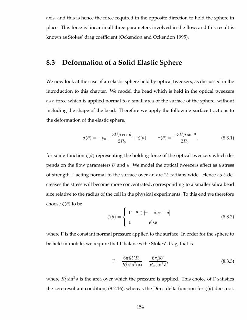
axis, and this is hence the force required in the opposite direction to hold the sphere in

place. This force is linear in all three parameters involved in the flow, and this result is

known as Stokes’ drag coefficient (Ockendon and Ockendon 1995).

8.3 Deformation of a Solid Elastic Sphere

We now look at the case of an elastic sphere held by optical tweezers, as discussed in the

introduction to this chapter. We model the bead which is held in the optical tweezers

as a force which is applied normal to a small area of the surface of the sphere, without

including the shape of the bead. Therefore we apply the following surface tractions to

the deformation of the elastic sphere,

σ(θ) = −p0 +3Uµ cos θ

2R0+ ζ(θ), τ(θ) =

−3Uµ sin θ

2R0, (8.3.1)

for some function ζ(θ) representing the holding force of the optical tweezers which de-

pends on the flow parameters U and µ. We model the optical tweezers effect as a stress

of strength Γ acting normal to the surface over an arc 2δ radians wide. Hence as δ de-

creases the stress will become more concentrated, corresponding to a smaller silica bead

size relative to the radius of the cell in the physical experiments. To this end we therefore

choose ζ(θ) to be

ζ(θ) =

Γ θ ∈ [π − δ, π + δ]

0 else(8.3.2)

where Γ is the constant normal pressure applied to the surface. In order for the sphere to

be held immobile, we require that Γ balances the Stokes’ drag, that is

Γ =6πµUR0

R20 sin2(δ)

=6πµU

R0 sin2 δ, (8.3.3)

where R20 sin2 δ is the area over which the pressure is applied. This choice of Γ satisfies

the zero resultant condition, (8.2.16), whereas the Direc delta function for ζ(θ) does not.

154

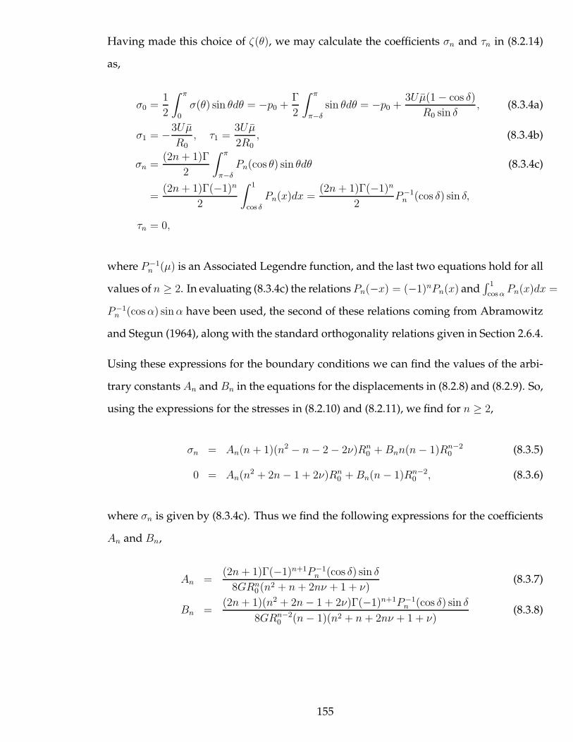
Having made this choice of ζ(θ), we may calculate the coefficients σn and τn in (8.2.14)

as,

σ0 =1

2

∫ π

0

σ(θ) sin θdθ = −p0 +Γ

2

∫ π

π−δ

sin θdθ = −p0 +3Uµ(1 − cos δ)

R0 sin δ, (8.3.4a)

σ1 = −3Uµ

R0, τ1 =

3Uµ

2R0, (8.3.4b)

σn =(2n+ 1)Γ

2

∫ π

π−δ

Pn(cos θ) sin θdθ (8.3.4c)

=(2n+ 1)Γ(−1)n

2

∫ 1

cos δ

Pn(x)dx =(2n+ 1)Γ(−1)n

2P−1

n (cos δ) sin δ,

τn = 0,

where P−1n (µ) is an Associated Legendre function, and the last two equations hold for all

values of n ≥ 2. In evaluating (8.3.4c) the relations Pn(−x) = (−1)nPn(x) and∫ 1

cos αPn(x)dx =

P−1n (cosα) sinα have been used, the second of these relations coming from Abramowitz

and Stegun (1964), along with the standard orthogonality relations given in Section 2.6.4.

Using these expressions for the boundary conditions we can find the values of the arbi-

trary constants An and Bn in the equations for the displacements in (8.2.8) and (8.2.9). So,

using the expressions for the stresses in (8.2.10) and (8.2.11), we find for n ≥ 2,

σn = An(n + 1)(n2 − n− 2 − 2ν)Rn0 +Bnn(n− 1)Rn−2

0 (8.3.5)

0 = An(n2 + 2n− 1 + 2ν)Rn0 +Bn(n− 1)Rn−2

0 , (8.3.6)

where σn is given by (8.3.4c). Thus we find the following expressions for the coefficients

An and Bn,

An =(2n+ 1)Γ(−1)n+1P−1

n (cos δ) sin δ

8GRn0 (n2 + n+ 2nν + 1 + ν)

(8.3.7)

Bn =(2n+ 1)(n2 + 2n− 1 + 2ν)Γ(−1)n+1P−1

n (cos δ) sin δ

8GRn−20 (n− 1)(n2 + n + 2nν + 1 + ν)

(8.3.8)

155

Considering the cases when n = 0, 1 separately, we find the following two constants,

A0 = − σ0

4G(1 + ν)= − 1

4G(1 + ν)

[

−p0 +Γ(1 − cos δ)

2

]

(8.3.9)

A1 =τ1

4GR0(1 + ν)=

3Uµ

8GR20(1 + ν)

(8.3.10)

The coefficient B1 represents a rigid body motion corresponding to the displacements

uR = B1 cos θ, uθ = B1 sin θ, and hence does not produce any stresses and may be super-

imposed on any stress-produced deformation, and therefore we set B1 = 0 without any

loss of generality. We note that in the expressions above, the constants U, µ and G only

occur in the formulae for the displacements and stresses in the dimensionless combina-

tion η = UµGR0

, and hence it is this ratio which is relevant rather than the individual values.

An equivalent ratio is denoted the capillary number by Lac et al. (2007) and expresses the

relative importance of the fluid viscous stresses to the elastic property of the material,

and it is therefore the size of this number which determines how much the sphere de-

forms. Similarly, the initial radius of the sphere R0 only scales the values of the resulting

sphere and hence can be taken as unity without loss of generality.

8.3.1 Results

With all the arbitrary coefficients determined we may find the displacements, uR, uθ, as

a function of the coordinates (r, θ), and then plot the resulting deformed sphere after the

deformation.

To plot the deformed shape Mathematica was used to calculate the displacement u at the

surface of the sphere, then the values of x = X + u were plotted to give the deformed

sphere. For the infinite sums in (8.2.8) and (8.2.9) the first 42 terms were taken, as this

was sufficient to give smooth functions for the displacements without causing numer-

ical precision errors as was found when taking more terms. In the following, the dia-

grams shown are planes through the ‘sphere’ at a fixed value of φ, the complete deformed

sphere being made by revolving this plane around the z-axis as it has been assumed that

156

the resulting shape is axisymmetric. Figure 8.3.1 shows the undeformed sphere with a

-1.0 -0.5 0.5 1.0

-1.0

-0.5

0.5

1.0

Figure 8.3.1: Sphere of unit radius with bold arc corresponding to the area over whichthe restraining force is applied when δ = 0.1

bold arc corresponding to the δ radians where the force from the optical tweezers applies.

The exterior pressure, p0, does not enter the formulae for the stresses or the displacements

in the incompressible case when ν = 1/2. This stems from the fact that the pressure is

distributed evenly around the exterior of the sphere, and incompressibility implies that

no deformation is possible from such a pressure. When ν = 1/2 the deformation is

mostly concentrated around the optical tweezers force, with little change to the shape

of the sphere elsewhere. This can be seen clearly in figure 8.3.2, where the increase of

the external flow speed primarily increases the elongation of the ‘tendril’ on the nega-

tive z-axis with little significant change elsewhere. Varies of η which are less than 0.001

show very little deformation, and we may therefore see a posteriori that the assumptions

of linear elasticity are appropriate in this case. Note that ν = 1/2 corresponds to incom-

pressibility, though the cell shows a change of volume for η = 0.01, 0.03 and higher. This

is a consequence of the fact that the deformations are becoming large, and the specifi-

cation ν = 1/2 is only an approximation to the nonlinear requirement of conservation

157

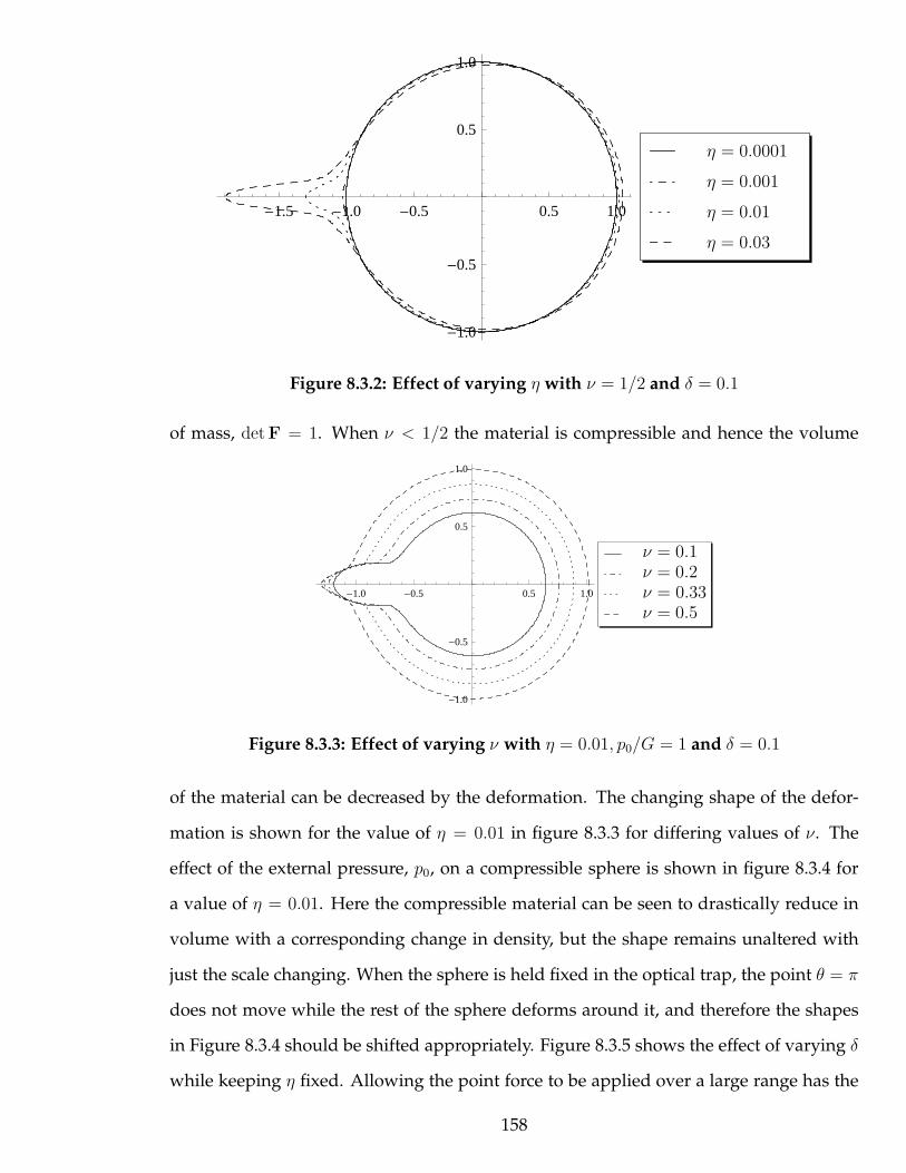
-1.5 -1.0 -0.5 0.5 1.0

-1.0

-0.5

0.5

1.0

η = 0.0001

η = 0.001

η = 0.01

η = 0.03

Figure 8.3.2: Effect of varying η with ν = 1/2 and δ = 0.1

of mass, detF = 1. When ν < 1/2 the material is compressible and hence the volume

-1.0 -0.5 0.5 1.0

-1.0

-0.5

0.5

1.0

ν = 0.1ν = 0.2ν = 0.33ν = 0.5

Figure 8.3.3: Effect of varying ν with η = 0.01, p0/G = 1 and δ = 0.1

of the material can be decreased by the deformation. The changing shape of the defor-

mation is shown for the value of η = 0.01 in figure 8.3.3 for differing values of ν. The

effect of the external pressure, p0, on a compressible sphere is shown in figure 8.3.4 for

a value of η = 0.01. Here the compressible material can be seen to drastically reduce in

volume with a corresponding change in density, but the shape remains unaltered with

just the scale changing. When the sphere is held fixed in the optical trap, the point θ = π

does not move while the rest of the sphere deforms around it, and therefore the shapes

in Figure 8.3.4 should be shifted appropriately. Figure 8.3.5 shows the effect of varying δ

while keeping η fixed. Allowing the point force to be applied over a large range has the

158

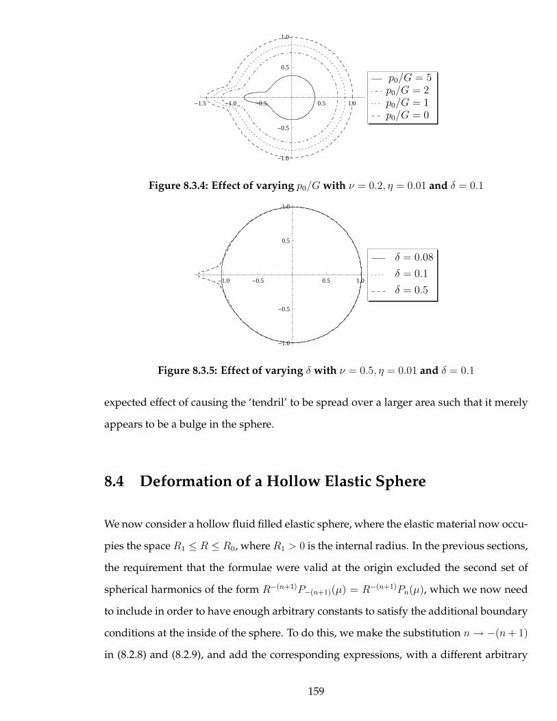
-1.5 -1.0 -0.5 0.5 1.0

-1.0

-0.5

0.5

1.0

p0/G = 5p0/G = 2p0/G = 1p0/G = 0

Figure 8.3.4: Effect of varying p0/G with ν = 0.2, η = 0.01 and δ = 0.1

-1.0 -0.5 0.5 1.0

-1.0

-0.5

0.5

1.0

δ = 0.08

δ = 0.1

δ = 0.5

Figure 8.3.5: Effect of varying δ with ν = 0.5, η = 0.01 and δ = 0.1

expected effect of causing the ‘tendril’ to be spread over a larger area such that it merely

appears to be a bulge in the sphere.

8.4 Deformation of a Hollow Elastic Sphere

We now consider a hollow fluid filled elastic sphere, where the elastic material now occu-

pies the space R1 ≤ R ≤ R0, where R1 > 0 is the internal radius. In the previous sections,

the requirement that the formulae were valid at the origin excluded the second set of

spherical harmonics of the form R−(n+1)P−(n+1)(µ) = R−(n+1)Pn(µ), which we now need

to include in order to have enough arbitrary constants to satisfy the additional boundary

conditions at the inside of the sphere. To do this, we make the substitution n→ −(n+ 1)

in (8.2.8) and (8.2.9), and add the corresponding expressions, with a different arbitrary

159

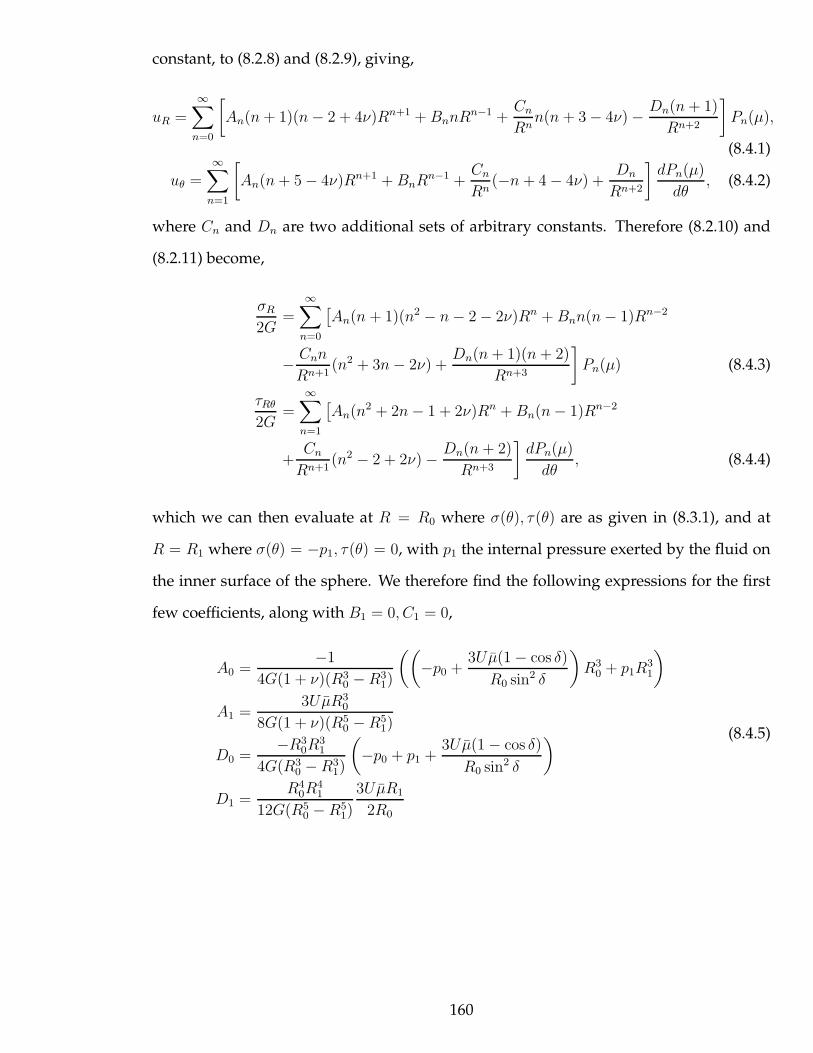
constant, to (8.2.8) and (8.2.9), giving,

uR =

∞∑

n=0

[

An(n+ 1)(n− 2 + 4ν)Rn+1 +BnnRn−1 +

Cn

Rnn(n + 3 − 4ν) − Dn(n+ 1)

Rn+2

]

Pn(µ),

(8.4.1)

uθ =∞∑

n=1

[

An(n+ 5 − 4ν)Rn+1 +BnRn−1 +

Cn

Rn(−n + 4 − 4ν) +

Dn

Rn+2

]dPn(µ)

dθ, (8.4.2)

where Cn and Dn are two additional sets of arbitrary constants. Therefore (8.2.10) and

(8.2.11) become,

σR

2G=

∞∑

n=0

[An(n + 1)(n2 − n− 2 − 2ν)Rn +Bnn(n− 1)Rn−2

− Cnn

Rn+1(n2 + 3n− 2ν) +

Dn(n+ 1)(n+ 2)

Rn+3

]

Pn(µ) (8.4.3)

τRθ

2G=

∞∑

n=1

[An(n2 + 2n− 1 + 2ν)Rn +Bn(n− 1)Rn−2

+Cn

Rn+1(n2 − 2 + 2ν) − Dn(n+ 2)

Rn+3

]dPn(µ)

dθ, (8.4.4)

which we can then evaluate at R = R0 where σ(θ), τ(θ) are as given in (8.3.1), and at

R = R1 where σ(θ) = −p1, τ(θ) = 0, with p1 the internal pressure exerted by the fluid on

the inner surface of the sphere. We therefore find the following expressions for the first

few coefficients, along with B1 = 0, C1 = 0,

A0 =−1

4G(1 + ν)(R30 −R3

1)

((

−p0 +3Uµ(1 − cos δ)

R0 sin2 δ

)

R30 + p1R

31

)

A1 =3UµR3

0

8G(1 + ν)(R50 −R5

1)

D0 =−R3

0R31

4G(R30 − R3

1)

(

−p0 + p1 +3Uµ(1 − cos δ)

R0 sin2 δ

)

D1 =R4

0R41

12G(R50 − R5

1)

3UµR1

2R0

(8.4.5)

160

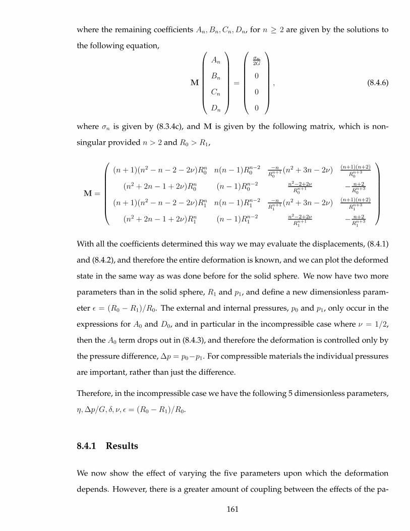
where the remaining coefficients An, Bn, Cn, Dn, for n ≥ 2 are given by the solutions to

the following equation,

M

An

Bn

Cn

Dn

=

σn

2G

0

0

0

, (8.4.6)

where σn is given by (8.3.4c), and M is given by the following matrix, which is non-

singular provided n > 2 and R0 > R1,

M =

(n+ 1)(n2 − n− 2 − 2ν)Rn0 n(n− 1)Rn−2

0−n

Rn+10

(n2 + 3n− 2ν) (n+1)(n+2)

Rn+30

(n2 + 2n− 1 + 2ν)Rn0 (n− 1)Rn−2

0n2−2+2ν

Rn+10

− n+2Rn+3

0

(n+ 1)(n2 − n− 2 − 2ν)Rn1 n(n− 1)Rn−2

1−n

Rn+11

(n2 + 3n− 2ν) (n+1)(n+2)

Rn+31

(n2 + 2n− 1 + 2ν)Rn1 (n− 1)Rn−2

1n2−2+2ν

Rn+11

− n+2Rn+3

1

With all the coefficients determined this way we may evaluate the displacements, (8.4.1)

and (8.4.2), and therefore the entire deformation is known, and we can plot the deformed

state in the same way as was done before for the solid sphere. We now have two more

parameters than in the solid sphere, R1 and p1, and define a new dimensionless param-

eter ǫ = (R0 − R1)/R0. The external and internal pressures, p0 and p1, only occur in the

expressions for A0 and D0, and in particular in the incompressible case where ν = 1/2,

then the A0 term drops out in (8.4.3), and therefore the deformation is controlled only by

the pressure difference, ∆p = p0−p1. For compressible materials the individual pressures

are important, rather than just the difference.

Therefore, in the incompressible case we have the following 5 dimensionless parameters,

η,∆p/G, δ, ν, ǫ = (R0 −R1)/R0.

8.4.1 Results

We now show the effect of varying the five parameters upon which the deformation

depends. However, there is a greater amount of coupling between the effects of the pa-

161

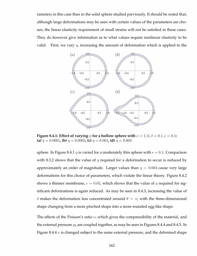
rameters in this case than in the solid sphere studied previously. It should be noted that,

although large deformations may be seen with certain values of the parameters are cho-

sen, the linear elasticity requirement of small strains will not be satisfied in these cases.

They do however give information as to what values require nonlinear elasticity to be

valid. First, we vary η, increasing the amount of deformation which is applied to the

-1.0 -0.5 0.5 1.0

-1.0

-0.5

0.5

1.0

-1.0 -0.5 0.5 1.0

-1.0

-0.5

0.5

1.0

-1.0 -0.5 0.5 1.0

-1.0

-0.5

0.5

1.0

-1.5 -1.0 -0.5 0.5 1.0

-1.0

-0.5

0.5

1.0

(a) (b)

(c) (d)

Figure 8.4.1: Effect of varying η for a hollow sphere with ν = 1/2, δ = 0.1, ǫ = 0.1:(a) η = 0.0001, (b) η = 0.0005, (c) η = 0.001, (d) η = 0.003

sphere. In Figure 8.4.1 η is varied for a moderately thin sphere with ǫ = 0.1. Comparison

with 8.3.2 shows that the value of η required for a deformation to occur is reduced by

approximately an order of magnitude. Larger values than η = 0.003 cause very large

deformations for this choice of parameters, which violate the linear theory. Figure 8.4.2

shows a thinner membrane, ǫ = 0.05, which shows that the value of η required for sig-

nificant deformations is again reduced. As may be seen in 8.4.3, increasing the value of

δ makes the deformation less concentrated around θ = π, with the three-dimensional

shape changing from a more pinched shape into a more rounded egg-like shape.

The effects of the Poisson’s ratio ν, which gives the compressibility of the material, and

the external pressure p0 are coupled together, as may be seen in Figures 8.4.4 and 8.4.5. In

Figure 8.4.4 ν is changed subject to the same external pressure, and the deformed shape

162

-1.0 -0.5 0.5 1.0

-1.0

-0.5

0.5

1.0

-1.0 -0.5 0.5 1.0

-1.0

-0.5

0.5

1.0

-1.0 -0.5 0.5 1.0

-1.0

-0.5

0.5

1.0

-1.5 -1.0 -0.5 0.5 1.0

-1.0

-0.5

0.5

1.0

(a) (b)

(c) (d)

Figure 8.4.2: Effect of varying η for a hollow sphere with ν = 1/2, δ = 0.1, ǫ = 0.05:(a) η = 0.0001, (b) η = 0.0005, (c) η = 0.001, (d) η = 0.003

-1.0 -0.5 0.5 1.0

-1.0

-0.5

0.5

1.0

-1.0 -0.5 0.5 1.0

-1.0

-0.5

0.5

1.0

-1.0 -0.5 0.5 1.0

-1.0

-0.5

0.5

1.0

-1.0 -0.5 0.5 1.0

-1.0

-0.5

0.5

1.0

(a) (b)

(c) (d)

Figure 8.4.3: Effect of varying δ for a hollow sphere with ν = 1/2, η = 0.001, ǫ = 0.1:(a) δ = 0.01, (b) δ = 0.1, (c) δ = 0.3, (d) δ = 0.5

is squeezed further when the material is more compressible, as expected. Figure 8.4.5

shows how increasing the external pressure has a very similar effect as decreasing ν.

The scaled thickness of the membrane, ǫ, plays a very significant role in the deformation.

Figure 8.4.6 shows how changing this thickness for a given value of η very markedly

163

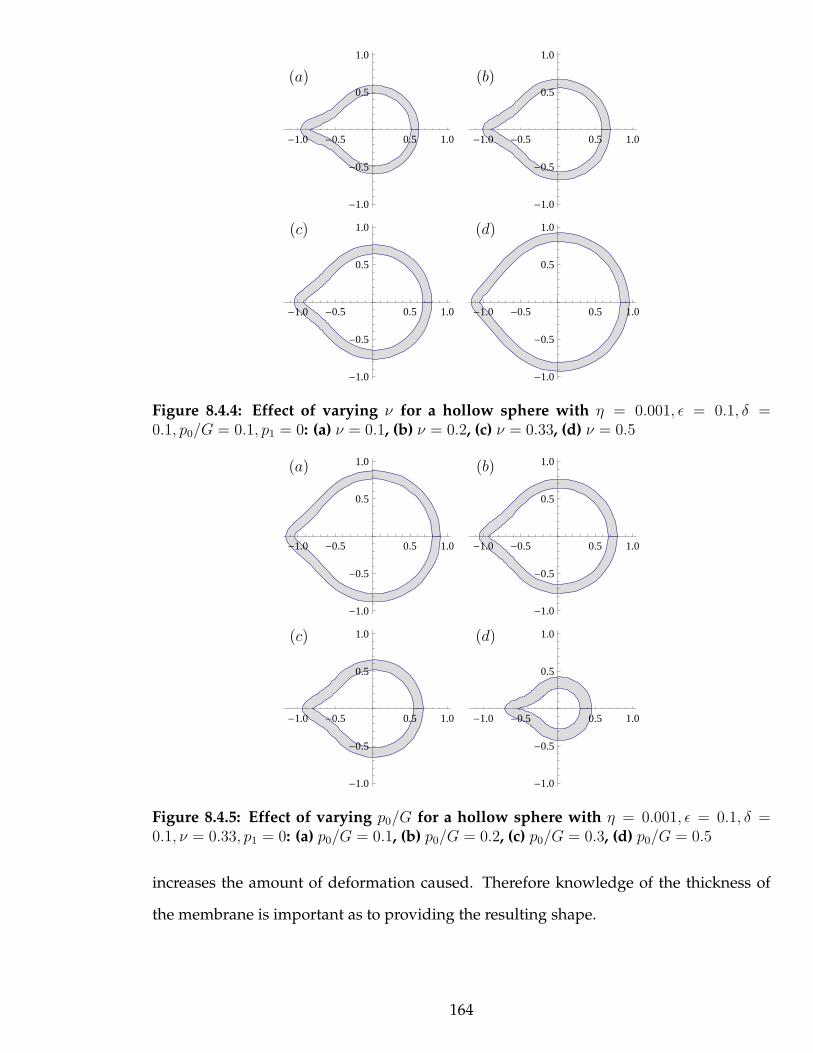
-1.0 -0.5 0.5 1.0

-1.0

-0.5

0.5

1.0

-1.0 -0.5 0.5 1.0

-1.0

-0.5

0.5

1.0

-1.0 -0.5 0.5 1.0

-1.0

-0.5

0.5

1.0

-1.0 -0.5 0.5 1.0

-1.0

-0.5

0.5

1.0

(a) (b)

(c) (d)

Figure 8.4.4: Effect of varying ν for a hollow sphere with η = 0.001, ǫ = 0.1, δ =0.1, p0/G = 0.1, p1 = 0: (a) ν = 0.1, (b) ν = 0.2, (c) ν = 0.33, (d) ν = 0.5

-1.0 -0.5 0.5 1.0

-1.0

-0.5

0.5

1.0

-1.0 -0.5 0.5 1.0

-1.0

-0.5

0.5

1.0

-1.0 -0.5 0.5 1.0

-1.0

-0.5

0.5

1.0

-1.0 -0.5 0.5 1.0

-1.0

-0.5

0.5

1.0

(a) (b)

(c) (d)

Figure 8.4.5: Effect of varying p0/G for a hollow sphere with η = 0.001, ǫ = 0.1, δ =0.1, ν = 0.33, p1 = 0: (a) p0/G = 0.1, (b) p0/G = 0.2, (c) p0/G = 0.3, (d) p0/G = 0.5

increases the amount of deformation caused. Therefore knowledge of the thickness of

the membrane is important as to providing the resulting shape.

164

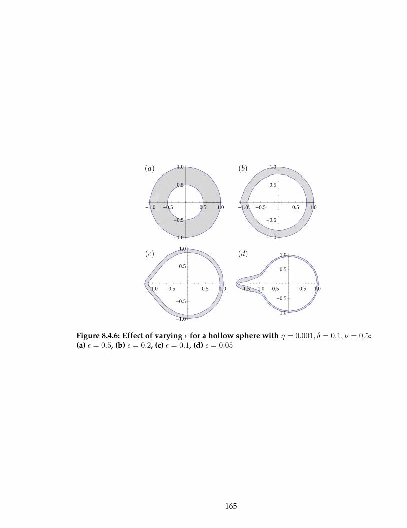
-1.0 -0.5 0.5 1.0

-1.0

-0.5

0.5

1.0

-1.0 -0.5 0.5 1.0

-1.0

-0.5

0.5

1.0

-1.0 -0.5 0.5 1.0

-1.0

-0.5

0.5

1.0

-1.5 -1.0 -0.5 0.5 1.0

-1.0

-0.5

0.5

1.0

(a) (b)

(c) (d)

Figure 8.4.6: Effect of varying ǫ for a hollow sphere with η = 0.001, δ = 0.1, ν = 0.5:(a) ǫ = 0.5, (b) ǫ = 0.2, (c) ǫ = 0.1, (d) ǫ = 0.05

165

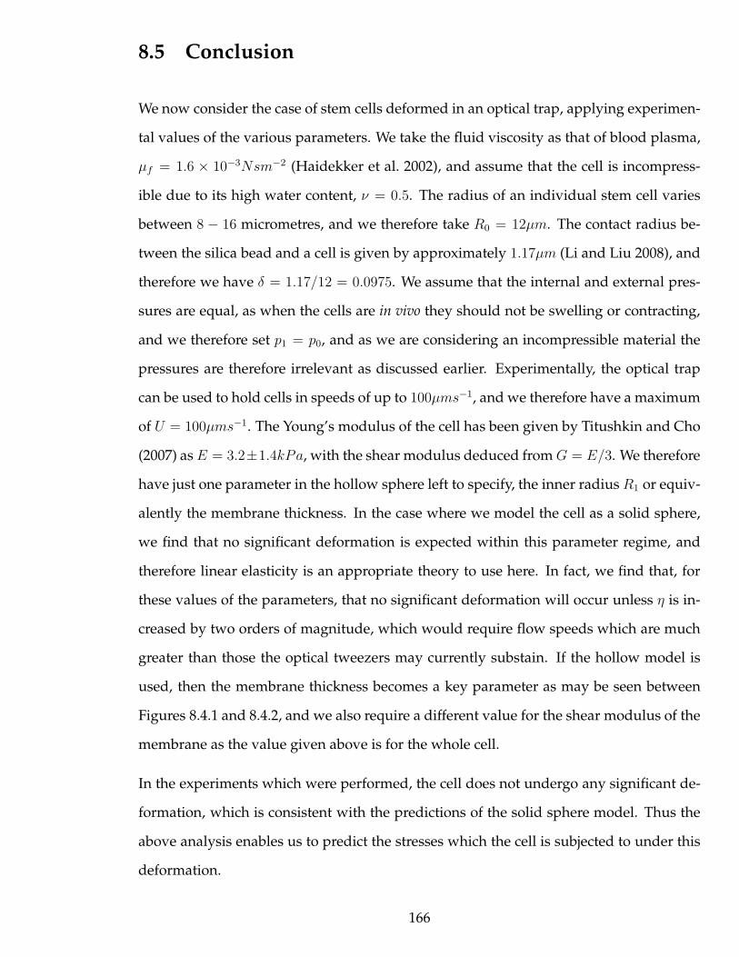
8.5 Conclusion

We now consider the case of stem cells deformed in an optical trap, applying experimen-

tal values of the various parameters. We take the fluid viscosity as that of blood plasma,

µf = 1.6 × 10−3Nsm−2 (Haidekker et al. 2002), and assume that the cell is incompress-

ible due to its high water content, ν = 0.5. The radius of an individual stem cell varies

between 8 − 16 micrometres, and we therefore take R0 = 12µm. The contact radius be-

tween the silica bead and a cell is given by approximately 1.17µm (Li and Liu 2008), and

therefore we have δ = 1.17/12 = 0.0975. We assume that the internal and external pres-

sures are equal, as when the cells are in vivo they should not be swelling or contracting,

and we therefore set p1 = p0, and as we are considering an incompressible material the

pressures are therefore irrelevant as discussed earlier. Experimentally, the optical trap

can be used to hold cells in speeds of up to 100µms−1, and we therefore have a maximum

of U = 100µms−1. The Young’s modulus of the cell has been given by Titushkin and Cho

(2007) as E = 3.2±1.4kPa, with the shear modulus deduced fromG = E/3. We therefore

have just one parameter in the hollow sphere left to specify, the inner radius R1 or equiv-

alently the membrane thickness. In the case where we model the cell as a solid sphere,

we find that no significant deformation is expected within this parameter regime, and

therefore linear elasticity is an appropriate theory to use here. In fact, we find that, for

these values of the parameters, that no significant deformation will occur unless η is in-

creased by two orders of magnitude, which would require flow speeds which are much

greater than those the optical tweezers may currently substain. If the hollow model is

used, then the membrane thickness becomes a key parameter as may be seen between

Figures 8.4.1 and 8.4.2, and we also require a different value for the shear modulus of the

membrane as the value given above is for the whole cell.

In the experiments which were performed, the cell does not undergo any significant de-

formation, which is consistent with the predictions of the solid sphere model. Thus the

above analysis enables us to predict the stresses which the cell is subjected to under this

deformation.

166

References

Abkarian, M., M. Faivre, and A. Viallat (2007). Swinging of red blood cells under shear

flow. Physical Review Letters 98(18), 188302.

Abramowitz, M. and I. A. Stegun (1964). Handbook of Mathematical Functions with For-

mulas, Graphs, and Mathematical Tables (ninth Dover printing, tenth GPO printing ed.).

New York: Dover.

Adkins, J. E. and R. S. Rivlin (1952). Large elastic deformations of isotropic materials. IX.

The deformation of thin shells. Philosophical Transactions of the Royal Society of London.

Series A, Mathematical and Physical Sciences 244(888), 505–531.

Afendikov, A. L. and T. J. Bridges (2001). Instability of the Hocking-Stewartson pulse

and its implications for three-dimensional Poiseuille flow. Proceedings: Mathematical,

Physical and Engineering Sciences 457(2006), 257–272.

Alastrue, V., E. Pena, M. Martınez, and M. Doblare (2007). Assessing the use of the

opening angle method to enforce residual stresses in patient-specific arteries. Annals of

Biomedical Engineering 35(10), 1821–1837.

Alexander, H. (1971). The tensile instability of an inflated cylindrical membrane as af-

fected by an axial load. International Journal of Mechanical Sciences 13, 87–95.

Alexander, J., R. Gardner, and C. Jones (1990). A topological invariant arising in the

stability analysis of travelling waves. fur die Reine und Angewandter Mathematik 410(1),

167–212.

167

Alexandrov, V. M. and D. A. Pozharskii (2001). Three-Dimensional Contact Problems. Solid

Mechanics and its Applications. Kluwer Academic Publishers.

Ananthakrishnan, R., J. Guck, F. Wottawah, S. Schinkinger, B. Lincoln, M. Romeyke, and

J. Kas (2005). Modelling the structural response of an eukaryotic cell in the optical

stretcher. Current Science 88, 1434–1440.

Andra, H., M. K. Warby, and J. R. Whiteman (2000). Contact problems of hyperelastic

membranes: Existence theory. Mathematical methods in the applied sciences 23(10), 865–

895.

Antman, S. S. (2005). Nonlinear problems of elasticity. Berlin: Springer-Verlag.

Baesu, E., R. E. Rudd, J. Belak, and M. McElfresh (2004). Continuum modeling of cell

membranes. International Journal of Non-Linear Mechanics 39(3), 369–377.

Bao, G. and S. Suresh (2003). Cell and molecular mechanics of biological materials. Nature

Materials 2(11), 715–725.

Barber, J. R. (2004). Elasticity (Second ed.). Kluwer Academic Publishers.

Barthes-Biesel, D. (1980). Motion of a spherical microcapsule freely suspended in a linear

shear flow. Journal of Fluid Mechanics 100, 831–853.

Barthes-Biesel, D. and J. Rallison (1981). The time-dependent deformation of a capsule

freely suspended in a linear shear flow. Journal of Fluid Mechanics 113, 251–267.

Benedict, R., A. S. Wineman, and W. H. Yang (1979). The determination of limiting pres-

sure in simultaneous elongation and inflation of nonlinear elastic tubes. International

Journal of Solids and Structures 15(3), 241–249.

Bertram, A. (2008). Elasticity and Plasticity of Large Deformations (Second ed.). Berlin:

Springer-Verlag.

Bhatnagar, P. L. (1979). Nonlinear waves in one-dimensional dispersive systems. Oxford.

168

Blyth, M. G. and C. Pozrikidis (2004). Solution space of axisymmetric capsules enclosed

by elastic membranes. European Journal of Mechanics/A Solids 23(5), 877–892.

Carroll, M. M. (1987). Pressure maximum behavior in inflation of incompressible elastic

hollow spheres and cylinders. Quarterly of Applied Mathematics 45, 141–154.

Chadwick, P. (1999). Continuum Mechanics: Concise Theory and Problems (Second ed.).

Dover Publications.

Chang, K. S. and W. L. Olbricht (1993). Experimental studies of the deformation and

breakup of a synthetic capsule in steady and unsteady simple shear flow. Journal of

Fluid Mechanics 250, 609–633.

Chater, E. and J. W. Hutchinson (1984). On the propagation of bulges and buckles. ASME

Journal of Applied Mechanics 51, 269–277.

Chen, Y. C. (1997). Stability and bifurcation of finite deformations of elastic cylindrical

membranes–Part I. Stability analysis. International Journal of Solids and Structures 34(14),

1735–1749.

Chen, Y.-C. and T. J. Healey (1991). Bifurcation to pear-shaped equilibria of pressurized

spherical membranes. International Journal of Non-linear Mechanics 26(3), 279–291.

Chicurel, M. E., C. S. Chen, and D. E. Ingber (1998). Cellular control lies in the balance of

forces. Current Opinion in Cell Biology 10(2), 232–239.

Dao, M., C. T. Lim, and S. Suresh (2003). Mechanics of the human red blood cell deformed

by optical tweezers. Journal of the Mechanics and Physics of Solids 51(11-12), 2259–2280.

Deans, R. J. and A. B. Moseley (2000). Mesenchymal stem cells: biology and potential

clinical uses. Experimental Hematology 28(8), 875–84.

Epstein, M. and C. R. Johnston (2001). On the exact speed and amplitude of solitary

waves in fluid-filled elastic tubes. Proceedings of the Royal Society A 457, 1195–1213.

169

Erbay, H. A. and H. Demiray (1995). Finite axisymmetric deformations of elastic tubes:

An approximate method. Journal of Engineering Mathematics 29(5), 451–472.

Ericksen, J. L. (1975). Equilibrium of bars. Journal of Elasticity 5, 191–201.

Eringen, A. C. (1962). Nonlinear theory of continuous media. McGraw-Hill.

Evans, J. W. (1975). Nerve axon equations. IV. The stable and unstable impulse. Indiana

University Mathematics Journal 24, 1169–1190.

Farrell, O. J. and B. Ross (1963). Solved problems: gamma and beta functions, Legendre poly-

nomials, Bessel functions. Macmillan.

Fery, A. and R. Weinkamer (2007). Mechanical properties of micro-and nanocapsules:

Single-capsule measurements. Polymer 48, 7221–7235.

Finken, R. and U. Seifert (2006). Wrinkling of microcapsules in shear flow. Journal of

Physics: Condensed Matter 18, 185–191.

Foo, J. J., K. K. Liu, and V. Chan (2004). Viscous drag of deformed vesicles in optical trap:

Experiments and simulations. AIChE Journal 50(1), 249–254.

Frangos, J. A., L. V. McIntire, and S. G. Eskin (1988). Shear stress induced stimulation of

mammalian cell metabolism. Biotechnology and bioengineering 32(8), 1053–1060.

Fu, Y. B. (2001). Perturbation methods and nonlinear stability analysis. In Y. B. Fu and

R. W. Ogden (Eds.), Nonlinear Elasticity: Theory and Applications, pp. 345–391. Cam-

bridge University Press.

Fu, Y. B. and A. T. Il’ichev (2010). Solitary waves in fluid filled elastic tubes: existence,

persistence and the role of axial displacement. IMA Journal of Applied Mathematics 75(2),

257–268.

Fu, Y. B., S. P. Pearce, and K. K. Liu (2008). Post-bifurcation analysis of a thin-walled

hyperelastic tube under inflation. International Journal of Non-Linear Mechanics 43(8),

697–706.

170

Fung, Y. (1993). Biomechanics: Mechanical Properties of Living Tissues. Springer.

Gee, M. W., C. Reeps, H. H. Eckstein, and W. A. Wall (2009). Prestressing in finite de-

formation abdominal aortic aneurysm simulation. Journal of Biomechanics 42(11), 1732–

1739.

Gent, A. N. (1996). A new constitutive relation for rubber. Rubber chemistry and technol-

ogy 69(1), 59–61.

Gent, A. N. (2005). Elastic instabilities in rubber. International Journal of Non-linear Me-

chanics 40, 165–175.

Goncalves, P. B., D. Pamplona, and S. R. X. Lopes (2008). Finite deformations of an

initially stressed cylindrical shell under internal pressure. International Journal of Me-

chanical Sciences 50(1), 92–103.

Green, A. E. and J. E. Adkins (1960). Large Elastic Deformations and Nonlinear Continuum

Mechanics. Clarendon Press.

Guck, J., R. Ananthakrishnan, H. Mahmood, T. J. Moon, C. C. Cunningham, and J. Kas

(2001). The optical stretcher: A novel laser tool to micromanipulate cells. Biophysical

Journal 81(2), 767–784.

Haidekker, M. A., A. G. Tsai, T. Brady, H. Y. Stevens, J. A. Frangos, E. Theodorakis, and

M. Intaglietta (2002). A novel approach to blood plasma viscosity measurement us-

ing fluorescent molecular rotors. American Journal of Physiology- Heart and Circulatory

Physiology 282(5), H1609.

Haughton, D. M. (1980). Post-bifurcation of perfect and imperfect spherical elastic mem-

branes. International Journal of Solids and Structures 16(12), 1123–1134.

Haughton, D. M. (2001). Elastic membranes. In Y. B. Fu and R. W. Ogden (Eds.), Nonlinear

Elasticity: Theory and Applications, pp. 233–267. Cambridge University Press.

171

Haughton, D. M. (2009). Evaluation of eigenfunctions from compound matrix variables

in non-linear elasticity–II. Sixth order systems. Journal of Computational Physics 36, 659–

668.

Haughton, D. M. and R. W. Ogden (1978a). On the incremental equations in non-linear

elasticity. I. Membrane theory. Journal of the Mechanics and Physics of Solids 26, 93–110.

Haughton, D. M. and R. W. Ogden (1978b). On the incremental equations in non-linear

elasticity. II. Bifurcation of pressurized spherical shells. Journal of the Mechanics and

Physics of Solids 26, 111–138.

Haughton, D. M. and R. W. Ogden (1979a). Bifurcation of inflated circular cylinders of

elastic material under axial loading. I. Membrane theory for thin-walled tubes. Journal

of the Mechanics and Physics of Solids 27, 179–212.

Haughton, D. M. and R. W. Ogden (1979b). Bifurcation of inflated circular cylinders of

elastic material under axial loading. II. Exact theory for thick-walled tubes. Journal of

the Mechanics and Physics of Solids 27, 489–512.

Henon, S., G. Lenormand, A. Richert, and F. Gallet (1999). A new determination of the

shear modulus of the human erythrocyte membrane using optical tweezers. Biophysical

Journal 76(2), 1145–1151.

Hobson, E. W. (1931). The theory of spherical and ellipsoidal harmonics. Cambridge Univer-

sity Press.

Holzapfel, G. A. (2000). Nonlinear Solid Mechanics: A Continuum Approach for Engineering.

WileyBlackwell.

Holzapfel, G. A., T. C. Gasser, and R. W. Ogden (2000). A new constitutive framework

for arterial wall mechanics and a comparative study of material models. Journal of

elasticity 61(1), 1–48.

Horgan, C. O. and G. Saccomandi (2003). A description of arterial wall mechanics

172

using limiting chain extensibility constitutive models. Biomechanics and Modeling in

Mechanobiology 1(4), 251–266.

Horgan, C. O. and G. Saccomandi (2006). Phenomenological hyperelastic strain-

stiffening constitutive models for rubber. Rubber Chemistry Technology 79, 152–169.

Howell, P., G. Kozyreff, and J. R. Ockendon (2009). Applied solid mechanics. Cambridge

University Press.

Humphrey, J. D. (1998). Review: Computer methods in membrane biomechanics. Com-

puter Methods in Biomechanics and Biomedical Engineering 1(3), 171.

Humphrey, J. D. (2003). Review paper: Continuum biomechanics of soft biological tis-

sues. Proceedings: Mathematical, Physical and Engineering Sciences 459, 3–46.

Humphrey, J. D., J. F. Eberth, W. W. Dye, and G. R. L. (2009). Fundamental role of axial

stress in compensatory adaptations by arteries. Journal of Biomechanics 42(1), 1–8.

Hutchinson, J. W. and K. W. Neale (1983). Neck propagation. Journal of the Mechanics and

Physics of Solids 31(5), 405–426.

Ingber, D. E. (2003). Cell structure and hierarchical systems biology. Journal of Cell Sci-

ence 116, 1157–73.

Jenkins, J. T. (1977). The equations of mechanical equilibrium of a model membrane.

SIAM Journal on Applied Mathematics 32(4), 755–764.

Jian-Guo, H. and O. Y. Zhong-Can (1993). Shape equations of the axisymmetric vesicles.

Physical Review E 47(1), 461–467.

Kanner, L. M. and C. O. Horgan (2007). Elastic instabilities for strain-stiffening rubber-

like spherical and cylindrical thin shells under inflation. International Journal of Non-

Linear Mechanics 42(2), 204–215.

Kydoniefs, A. D. (1969). Finite axisymmetric deformations of an initially cylindrical elas-

tic membrane enclosing a rigid body. The Quarterly Journal of Mechanics and Applied

Mathematics 22(3), 319–333.

173

Kydoniefs, A. D. and A. J. M. Spencer (1987). Finite deformation analysis of a thin-walled

tube sliding on a rough rigid rod. Journal of Engineering Mathematics 21(4), 363–377.

Kyriakides, S. and C. Babcock (1981). Experimental determination of the propagation

pressure of circular pipes. Journal of Pressure Vessel Technology 103, 328–336.

Kyriakides, S. and Y. C. Chang (1990). On the initiation of a long elastic tube in the

presence of axial load. International Journal of Solids and Structures 26, 975–991.

Kyriakides, S. and Y. C. Chang (1991). The initiation and propagation of a localized

instability in an inflated elastic tube. International Journal of Solids and Structures 27(9),

1113–1137.

Lac, E., A. Morel, and D. Barthes-Biesel (2007). Hydrodynamic interaction between two

identical capsules in simple shear flow. Journal of Fluid Mechanics 573, 149–169.

Landau, L. D. and E. M. Lifshitz (1986). Course of theoretical physics. vol. 7: Theory of

elasticity. (Third ed.). Butterworth-Heinemann.

Le Dret, H. and A. Raoult (1996). The membrane shell model in nonlinear elasticity: a

variational asymptotic derivation. Journal of Nonlinear Science 6(1), 59–84.

Learoyd, B. M. and M. G. Taylor (1966). Alterations with age in the viscoelastic properties

of human arterial walls. Circulation Research 18(3), 278.

Li, C. and K. K. Liu (2008). Nanomechanical characterization of red blood cells using

optical tweezers. Journal of Materials Science: Materials in Medicine 19(4), 1529–1535.

Li, C., Y. P. Liu, K. K. Liu, and J. H. Hsieh (2004). A parameter study of the material

properties in the vesicle–fluid interaction. Computational Materials Science 30(3-4), 504–

510.

Li, X. and D. J. Steigmann (1995). Point loads on a hemispherical elastic membrane.

International Journal of Non-Linear Mechanics 30(4), 569–581.

174

Libai, A. and J. G. Simmonds (1998). The nonlinear theory of elastic shells. Cambridge Univ

Press.

Lim, C. T., M. Dao, S. Suresh, C. H. Sow, and K. T. Chew (2004). Large deformation of

living cells using laser traps. Acta Materialia 52(7), 1837–1845.

Lim, C. T., E. H. Zhou, and S. T. Quek (2006). Mechanical models for living cells: A

review. Journal of biomechanics 39(2), 195–216.

Liu, Y. P., C. Li, K. K. Liu, and A. C. K. Lai (2006). The deformation of an erythrocyte

under the radiation pressure by optical stretch. Journal of Biomechanical Engineering 128,

830.

Lur’e, A. I. (1964). Three-dimensional Problems of the Theory of Elasticity. Interscience Pub-

lishers.

MacRobert, T. M. (1947). Spherical Harmonics. Methuen & Co. Ltd.

McCormick, S. M., S. G. Eskin, L. V. McIntire, C. L. Teng, C. M. Lu, C. G. Russell, and

K. K. Chittur (2001). DNA microarray reveals changes in gene expression of shear

stressed human umbilical vein endothelial cells. Proceedings of the National Academy of

Sciences 98(16), 8955–8960.

McMahon, H. and J. Gallop (2005). Membrane curvature and mechanisms of dynamic

cell membrane remodelling. Nature 438(7068), 590–596.

Muller, I. and P. P. Strehlow (2004). Rubber and Rubber Balloons: Paradigms of Thermody-

namics. Springer-Verlag.

Nadler, B. and M. B. Rubin (2009). Analysis of constitutive assumptions for the strain

energy of a generalized elastic membrane in a nonlinear contact problem. Journal of

Elasticity 97(1), 77–95.

Naghdi, P. M. (1972). The theory of shells and plates. In C. Trusdell (Ed.), Flugge’s Hand-

buch der Physik, Volume VI, pp. 425–460. Springer-Verlag.

175

Needleman, A. (1976). Necking of pressurized spherical membranes. Journal of the Me-

chanics and Physics of Solids 24, 339–359.

Needleman, A. (1977). Inflation of spherical rubber balloons. International Journal of Solids

and Structures 13(5), 409–421.

Ng, B. S. and W. H. Reid (1985). The compound matrix method for ordinary differential

systems. Journal of Computational Physics 58(2), 209–228.

Ockendon, H. and J. Ockendon (1995). Viscous Flow. Cambridge University Press.

Ogden, R. W. (1972). Large deformation isotropic elasticity-on the correlation of theory

and experiment for incompressible rubberlike solids. Proceedings of the Royal Society of

London. Series A, Mathematical and Physical Sciences 326(1567), 565–584.

Ogden, R. W. (1997). Non-linear elastic deformations. Dover Publications.

Ogden, R. W., G. Saccomandi, and I. Sgura (2006). On worm-like chain models within the

three-dimensional continuum mechanics framework. Proceedings of the Royal Society A:

Mathematical, Physical and Engineering Science 462(2067), 749.

Pamplona, D., P. Goncalves, M. Davidovich, and W. H. I. (2001). Finite axisymmetric

deformations of an intially stressed fluid-filled membrane. International Journal of Solids

and Structures 38, 2033–2047.

Pamplona, D. C. and C. R. Calladine (1993). The mechanics of axially symmetric lipo-

somes. Journal of Biomechanical Engineering 115, 149.

Pamplona, D. C., P. B. Goncalves, and S. R. X. Lopes (2006). Finite deformations of

cylindrical membrane under internal pressure. International Journal of Mechanical Sci-

ences 48(6), 683–696.

Pearce, S. P. and Y. B. Fu (2010). Characterisation and stability of localised

bulging/necking in inflated membrane tubes. IMA Journal of Applied Mathematics (in

press).

176

Pipkin, A. (1968). Integration of an equation in membrane theory. Zeitschrift fur Ange-

wandte Mathematik und Physik (ZAMP) 19(5), 818–819.

Pipkin, A. C. (1986). The relaxed energy density for isotropic elastic membranes. IMA

Journal of Applied Mathematics 36(1), 85.

Pozrikidis, C. (2001). Interfacial dynamics for stokes flow. Journal of Computational

Physics 169(2).

Pozrikidis, C. (2003). Shell theory for capsules and cells. In C. Pozrikidis (Ed.), Modeling

and Simulation of Capsules and Biological Cells, pp. 35–102. Chapman & Hall/CRC.

Preston, S. P., O. E. Jensen, and G. Richardson (2008). Buckling of an axisymmetric vesicle

under compression: The effects of resistance to shear. Quarterly Journal of Mechanics and

Applied Mathematics 61(1), 1–24.

Ramanujan, S. and C. Pozrikidis (1998). Deformation of liquid capsules enclosed by

elastic membranes in simple shear flow: Large deformations and the effect of fluid

viscosities. Journal of Fluid Mechanics 361, 117–143.

Shield, R. T. (1972). On the stability of finitely deformed elastic membranes. Part II:

Stability of inflated cylindrical and spherical membranes. Z. angew. Math. Phys 23, 16–

34.

Skalak, R., A. Tozeren, R. P. Zarda, and S. Chien (1973). Strain energy function of red

blood cell membranes. Biophysical Journal 13(3), 245.

Skotheim, J. M. and T. W. Secomb (2007). Red blood cells and other nonspherical cap-

sules in shear flow: Oscillatory dynamics and the tank-treading-to-tumbling transition.

Physical Review Letters 98(7), 78301.

Sokolnikoff, I. (1956). Mathematical theory of elasticity. McGraw-Hill.

Soper, R., N. P. O. Green, G. W. Stout, and D. J. Taylor (1990). Biological Science (Second

ed.). Cambridge University Press.

177

Spencer, A. J. M. (1980). Continuum mechanics. Longman Mathematical Texts.

Steigmann, D. J. (2001). Elements of the theory of elastic surfaces. In Y. B. Fu and R. W.

Ogden (Eds.), Nonlinear Elasticity: Theory and Applications, pp. 268–304. Cambridge

University Press.

Steigmann, D. J. (2007). Thin-plate theory for large elastic deformations. International

Journal of Non-Linear Mechanics 42(2), 233–240.

Steigmann, D. J. (2009). A concise derivation of membrane theory from three-

dimensional nonlinear elasticity. Journal of Elasticity 97(1), 97–101.

Steigmann, D. J. and R. W. Ogden (1999). Elastic surface-substrate interactions. Proceed-

ings: Mathematical, Physical and Engineering Sciences 455(1982), 437–474.

Titushkin, I. and M. Cho (2006). Distinct membrane mechanical properties of human

mesenchymal stem cells determined using laser optical tweezers. Biophysical Jour-

nal 90(7), 2582–2591.

Titushkin, I. and M. Cho (2007). Modulation of cellular mechanics during osteogenic

differentiation of human mesenchymal stem cells. Biophysical Journal 93(10), 3693–3702.

Tuzel, V. H. and H. A. Erbay (2004). The dynamic response of an incompressible non-

linearly elastic membrane tube subjected to a dynamic extension. International Journal

of Non-Linear Mechanics 39(4), 515–537.

Varga, O. H. (1966). Stress-strain behavior of elastic materials: selected problems of large defor-

mations. Interscience Publishers.

Walter, A., H. Rehage, and H. Leonhard (2001). Shear induced deformation of microcap-

sules: Shape oscillations and membrane folding. Colloids and Surfaces A 183, 123–132.

Watton, P. N., N. A. Hill, and M. Heil (2004). A mathematical model for the growth of the

abdominal aortic aneurysm. Biomechanics and modeling in mechanobiology 3(2), 98–113.

178

Watton, P. N., Y. Ventikos, and G. A. Holzapfel (2009). Modelling the mechanical response

of elastin for arterial tissue. Journal of Biomechanics 42(9), 1320–1325.

Yin, W. L. (1977). Non-uniform inflation of a cylindrical elastic membrane and direct

determination of the strain energy function. Journal of Elasticity 7(3), 265–282.

Zhang, H. and K. Liu (2008). Optical tweezers for single cells. Journal of the Royal Society

Interface 5(24), 671.

Zhong-Can, O. Y. and W. Helfrich (1989). Bending energy of vesicle membranes: General

expressions for the first, second, and third variation of the shape energy and applica-

tions to spheres and cylinders. Physical Review A 39(10), 5280–5288.

Zhu, Y., X. Y. Luo, and R. W. Ogden (2008). Asymmetric bifurcations of thick-walled

circular cylindrical elastic tubes under axial loading and external pressure. International

Journal of Solids and Structures 45(11-12), 3410–3429.

179