Bifurcations

We have already seen how the loss of sti!ness in a linear oscillator leadsto instability. In a practical situation the sti!ness may not degrade in alinear fashion, and instability may not lead to solutions that lose stabilitycompletely. The behavior of the linear oscillator provides an informativelocal view of behavior, but in a practical situation we might expectnonlinear e!ects to limit the response in some way. Bifurcation theorycan be used to classify instability phenomena based on generic behavior.In other words, as a control parameter is varied, e.g., the axial load on astructure, what happens to a system as a critical condition is reached?

Clearly the passage of an eigenvalue through to the positive real halfplane leads to a qualitative change in the phase portrait, i.e., thebehavior of trajectories in the local vicinity of an equilibrium point. As aparameter is (slowly) varied, the response of a system changes (oftengradually), but it is the qualitative change in the dynamics that isclassified as a bifurcation. Although an elementary classification ofbifurcations is based on a one-dimensional description, we will focusattention on two-dimensions (which are fundamentally one-dimensional,based on center manifold theory), since we are primarily interested inoscillations which result from application of Newton’s second law tostructural (mechanical) systems.

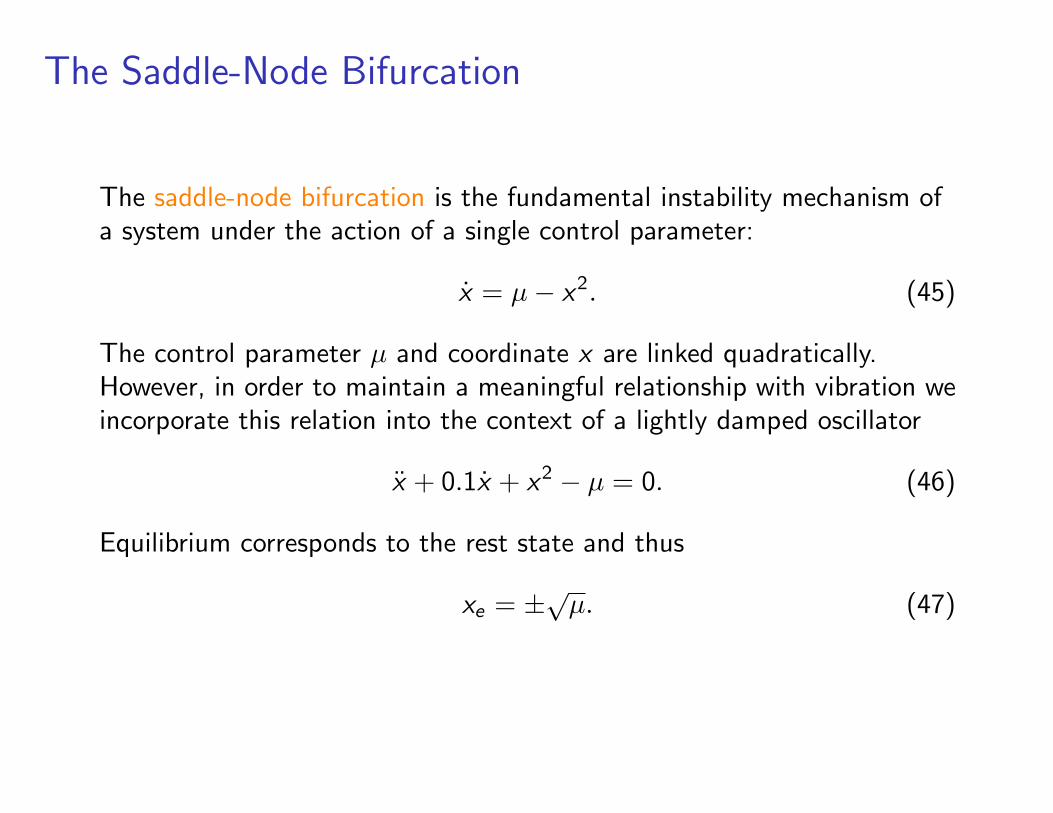
The Saddle-Node Bifurcation

The saddle-node bifurcation is the fundamental instability mechanism ofa system under the action of a single control parameter:

x = µ! x2. (45)

The control parameter µ and coordinate x are linked quadratically.However, in order to maintain a meaningful relationship with vibration weincorporate this relation into the context of a lightly damped oscillator

x + 0.1x + x2 ! µ = 0. (46)

Equilibrium corresponds to the rest state and thus

xe = ±"µ. (47)

The stability of these equilibria can be determined in a number of ways,and we start by considering the oscillations resulting from a smallperturbation. Let x = xe + !, where ! is a small deviation fromequilibrium. Placing this in equation (46), we get

! + 0.1! + x2e + 2xe! + !2 ! µ = 0. (48)

By definition x2e ! µ = 0, and neglecting !2 (since ! is small) we obtain

! + 0.1! + 2xe! = 0. (49)

This describes the dynamic response of small perturbations aboutequilibrium. Substituting in the expression for equilibrium, equation (47),results in

! + 0.1! ± 2"µ! = 0. (50)

Taking the positive sign we have a response which oscillates with afrequency a little less than "2

n = 2"µ. The damping causes the motion

to decay back to equilibrium.

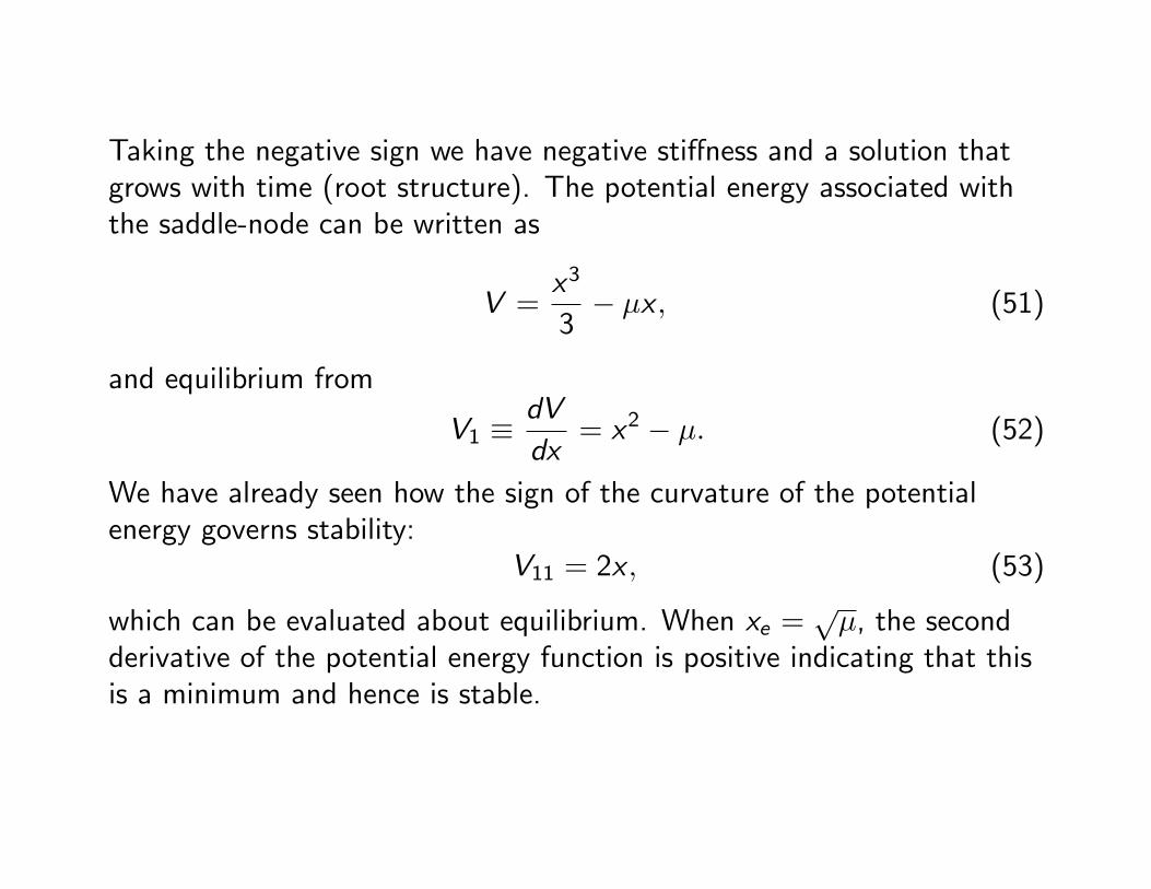
Taking the negative sign we have negative sti!ness and a solution thatgrows with time (root structure). The potential energy associated withthe saddle-node can be written as

V =x3

3! µx , (51)

and equilibrium from

V1 #dV

dx= x2 ! µ. (52)

We have already seen how the sign of the curvature of the potentialenergy governs stability:

V11 = 2x , (53)

which can be evaluated about equilibrium. When xe ="µ, the second

derivative of the potential energy function is positive indicating that thisis a minimum and hence is stable.

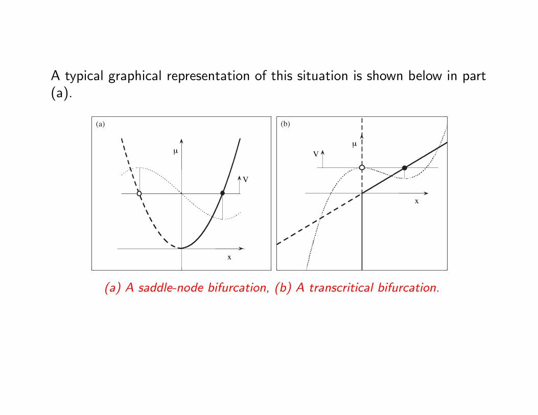
A typical graphical representation of this situation is shown below in part(a).

µ

x

V

(a)

µ

x

V

(b)

(a) A saddle-node bifurcation, (b) A transcritical bifurcation.

Suppose we have a system with a relatively large positive µ. In this casethere is a stable and an unstable equilibrium, characterized by a localminimum and a local maximum of the underlying potential energyrespectively. We can imagine the oscillations of a small ball rolling onthis potential energy surface (shown dotted in the previous slide). As thevalue of µ is reduced the two equilibria come together (the frequency ofsmall oscillations will decrease and e!ective damping increases) as thepotential surface flattens out. Just prior to coalescence the stableequilibrium can be thought of as a node, and the unstable equilibriumremains a saddle. Hence their approach (at the critical point) is called asaddle-node bifurcation. No equilibria exist for negative µ and trajectorieswould simply be swept away. This instability is also sometimes referred toas a fold or limit point.

Bifurcations from a Trivial Equilibrium

Although the saddle-node is the key stability transition in a system underthe action of a single control, there are many systems in mechanics inwhich some kind of initial symmetry is present. An example is thetranscritical bifurcation. In the context of a second order ordinarydi!erential equation we can write

x + 0.1x + x2 ! µx = 0. (54)

Following the same approach as for the saddle-node we obtain thesituation illustrated in part (b) of the previous figure. Here, there is afundamental (trivial) equilibrium for negative µ which loses stability as µpasses the through the origin (from negative to positive). The otherequilibrium becomes stable at this point and deflection occurs in thepositive x direction.

The final pair of bifurcations are associated with the loss of stability ofthe trivial solution and have global symmetry. They represent animportant class of instability in structural mechanics: super- andsub-critical pitchfork bifurcations. For the super-critical pitchforkbifurcation we can consider the oscillator

x + 0.1x + x3 ! µx = 0. (55)

Again, we observe the xe = 0 solution, which is stable for µ < 0. Atµ = 0 a secondary equilibrium intersects the fundamental and it can beshown that the two (symmetric) non-trivial solutions are stable. Thissituation corresponds to the classic double-well potential which is alsoshown superimposed for a specific (positive) value for µ.

µ

x

V

(a)µ

x

V

(b)

(a) A super-critical pitchfork bifurcation, (b) A sub-critical pitchforkbifurcation.

The corresponding sub-critical pitchfork bifurcation:

x + 0.1x + x3 + µx = 0, (56)

is shown in part(b).

In this case, suppose we start from a negative value of µ. The trivialequilibrium is again stable but now, when the critical point is reached, thesystem becomes completely unstable. Furthermore, as the critical point isapproached, the potential energy maxima associated with the adjacentsaddles start to erode the size of allowable perturbations. This is animportant consequence of the nonlinearity in the system. Although theselast two bifurcations have the same stable trivial equilibrium and criticalpoint, they have quite di!erent consequences if encountered in practice.Hence, they are sometimes characterized as safe or unsafe according towhether a local, or adjacent, post-critical stable equilibrium is available.

Initial Imperfections

It has already been mentioned that initial geometric imperfections or loadeccentricities may have a relatively profound e!ect on stability. We shallconsider this type of e!ect and its influence on the super-criticalpitchfork. Incorporating a small o!set causes equation (55) to be alteredto

x + 0.1x + x3 ! µx + # = 0, (57)

where # is a small parameter, which breaks the symmetry.

Part (a) shows how the instability transition is changed.

µ

x

V

(a)

µ

ω 2

(b)

(a) A perturbed super-critical pitchfork bifurcation, (b) Corresponding naturalfrequency (for the primary branch).

Now, for large negative µ we have a primary equilibrium slightly o!setfrom x = 0, and this simply grows as µ approaches, and then passesbeyond, the critical value for the perfect geometry (the origin). There isalso a complementary solution for negative x , but this wouldn’t ordinarilybe accessed under a natural loading history, i.e., as µ is monotonicallyincreased. However, the complementary solution does possess a criticalpoint, and this is actually a saddle-node bifurcation (which would beencountered if µ was initially large and x negative, and then µ werereduced). We also note the small tilt in the potential energy function.Furthermore, the complementary solution has an e!ect on very largeamplitude motion and strong disturbances, and this will be revisited later.

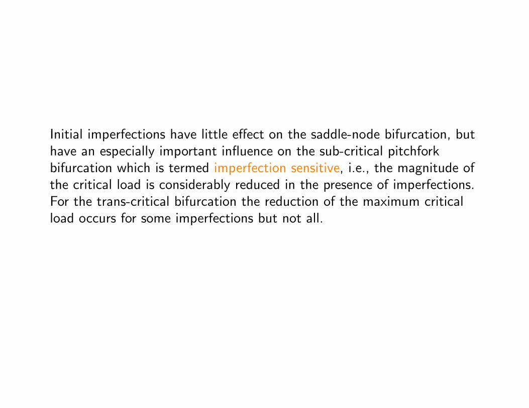
Initial imperfections have little e!ect on the saddle-node bifurcation, buthave an especially important influence on the sub-critical pitchforkbifurcation which is termed imperfection sensitive, i.e., the magnitude ofthe critical load is considerably reduced in the presence of imperfections.For the trans-critical bifurcation the reduction of the maximum criticalload occurs for some imperfections but not all.

A Simple Demonstration Model

Consider the slender, flexible system shown below (attributed to BrookeBenjamin).

l

qgravity

side view front view

board

cable

λ

λ

q

Schematic of an example bifurcation problem.

This simple system exhibits an unstable-symmetric (sub-critical pitchfork)bifurcation which subsequently stabilizes for large deflections.

We shall conduct a qualitative analysis of this system by associating aload parameter, µ, with the length of the cable (measured from thecritical value), and a displacement, q, associated with a generalout-of-plane deflection.The flexible cable is somewhat unusual since it possesses amoment-curvature relation that exhibits a softening spring e!ect, i.e., thesub-critical bifurcation manifests itself as a sudden motion from in-planeto a drooped out-of-plane position.

A qualitative form of the underlying potential function for this systemcan be written as

V =1

720q6 ! 1

24q4 ! 1

2µq2. (58)

That is, a function reflecting the global symmetry of the system andanticipated equilibria, which are given by the solutions of

V1 =1

120q5 ! 1

6q3 ! µq = 0. (59)

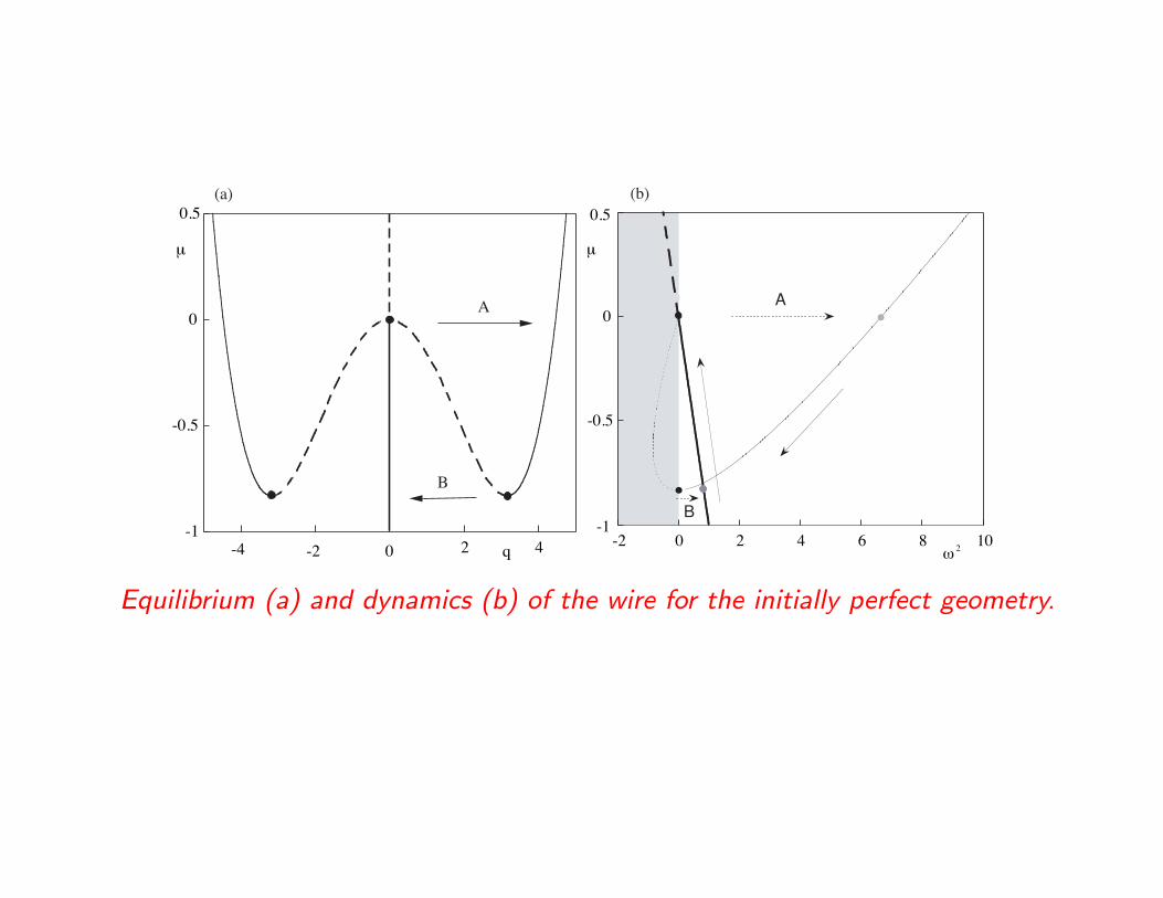
Thus equilibrium curves are given by:

q = 0

µ = !1

6q2 +

1

120q4, (60)

and are shown on the next page in part (a).

-1

-0.5

0

0.5

-4 -2 0 2 4

µ

q

(a)

A

B

-1

-0.5

0

0.5

-2 0 2 4 6 8 10

µ

ω 2

(b)

A

B

Equilibrium (a) and dynamics (b) of the wire for the initially perfect geometry.

The second derivative of potential energy is

V11 =1

24q4 ! 1

2q2 ! µ = 0, (61)

and evaluating this expression along the equilibrium paths of equation(60) we get

V f11 = !µ

V p11 =

1

24

!10±

"100 + 120$

"2

!1

2

!10±

"100 + 120$

"! µ. (62)

The sign of these expressions thus indicate stability. Assuming a simplequadratic form for the kinetic energy we can view equations (62) asrepresenting the natural frequencies. These are plotted as a function ofthe control (the length of the cable) in part (b). We see a linear decay asthe critical value is reached, followed by a finite jump to a higherfrequency associated with the heavily drooped equilibrium.

An initial imperfection can again be incorporated into the analysisstarting from

V =1

720q6 ! 1

24q4 ! 1

2µq2 + #q. (63)

Plots of these relations are shown in the figure below for somerepresentative initial imperfections.

-1

-0.5

0

0.5

-6 -4 -2 0 2 4 6

µ

ε = 0.01

ε = 0.3

ε = 0.1

q

(c)

-1

-0.5

0

0.5

-2 0 2 4 6 8 10

0.30.10.01

µ

ω 2

Imperfection, ε

(d)

Equilibrium (a) and dynamics (b) of the wire for the initially imperfectgeometry.