Bifurcations of phase portraits of pendulum withvibrating suspension point

A.I. Neishtadt1,2,∗, K. Sheng1

1 Loughborough University, Loughborough, LE11 3TU, UK2 Space Research Institute, Moscow, 117997, Russia

Abstract

We consider a simple pendulum whose suspension point undergoes fast vibrationsin the plane of motion of the pendulum. The averaged over the fast vibrations systemis a Hamiltonian system with one degree of freedom depending on two parameters. Wegive complete description of bifurcations of phase portraits of this averaged system.

1 Introduction

A simple pendulum with vibrating suspension point is a classical problem of perturbationtheory. The phenomenon of stabilisation of the upper vertical position of the pendulumby fast vertical vibrations of the suspension point was discovered by A. Stephenson [1, 2].In these papers the linearisation and reduction to the Mathieu equation is used. The caseof inclined vibrations of the suspension point is considered as well. Nonlinear theory wasdeveloped by N.N.Bogolyubov [3], who used the averaging method, and by P.L.Kapitsa, whohas developed a method of separation of slow and fast motions for this [4, 5] (see also [6]).Different aspects of this problem were discussed in many publications (see, e.g., [7] for adiscussion of geometric aspects, [8] for the case of arbitrary frequencies of vibrations, [9] forthe case of random vibrations). Generalisations to double- and multiple-link pendulums arecontained in [11, 12, 13]. It is noted in [10] that the problem is simplified by using averagingin Hamiltonian form. Such an approach is used, e.g., in [14, 15]. In [14] bifurcations ofthe phase portraits of the averaged problem for vertically vibrating suspension point aredescribed.

∗Corresponding author. E-mail addresses: A.Neishtadt@lboro.ac.uk (A.I.Neishtadt),shengkaicheng@yeah.net (K.Sheng)

1

arX

iv:1

605.

0944

8v2

[m

ath.

DS]

29

Sep

2016

We consider the case of arbitrary planar vibrations of the suspension point. We use theHamiltonian approach of [10] to construct the averaged system and give a complete descrip-tion of bifurcations of its phase portraits. Equations for equilibria of the averaged system inthis case are obtained in [16].

2 Hamiltonian of the problem

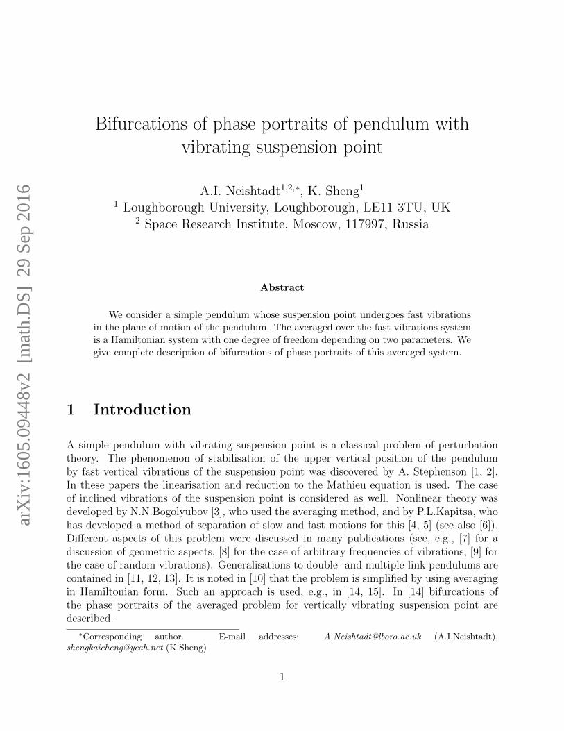
Consider a simple pendulum, Fig. 1, whose suspension point moves in the vertical planewhere the pendulum moves. Let l,m be length of the massless rod and mass of the bob forthis pendulum. Let ξ, η be horizontal and vertical Cartesian coordinates of the suspensionpoint. It is assumed that ξ, η are some given functions of time. Denote by ϕ the anglebetween the pendulum rod and the vertical line straight down.  

x

y

ξ(t)

η(t)

φ

Figure 1. A pendulum with vibrating suspension point.

Then the kinetic and potential energies of the bob are

T =1

2

[l2ϕ2 + 2lϕ(ξ cosϕ+ η sinϕ) + (ξ2 + η2)

], V = mg(η − l cosϕ) .

Here g is the gravity acceleration. The generalised momentum conjugate to ϕ is

p = ∂T/∂ϕ = ml2ϕ+ml(ξ cosϕ+ η sinϕ) .

Thus

ϕ =p

ml2− (ξ cosϕ+ η sinϕ)

l.

In order to obtain the Hamiltonian of the problem we should substitute this expression intoT + V and subtract terms which do not depend on p. Thus we get the Hamiltonian

H =1

2

(p2

ml2− 2

p(ξ cosϕ+ η sinϕ)

l+m(ξ cosϕ+ η sinϕ)2

)−mgl cosϕ .

2

3 Averaged Hamiltonian

Assume that ξ = εξ(ωt/ε), η = εη(ωt/ε), where ε is a small parameter, ξ(·), η(·) are 2π-periodic functions with zero average. Then ξ, η are values of order 1. In the system ofHamilton’s equations

ϕ = ∂H/∂p, p = −∂H/∂ϕ .

the right hand side is a fast oscillating function of time. In line with the averaging method[17], for an approximate description of dynamics of variables ϕ, p we average the Hamiltonian

H with respect to time t. Denote by A,B,C the averages of ξ2

2, η

2

2, and ξη, respectively.

Then the averaged Hamiltonian up to an additive constant is

H =1

2

p2

ml2+ V (ϕ), V = V (ϕ) =

m

2[(A−B) cos 2ϕ+ C sin 2ϕ]−mgl cosϕ .

The type of the phase portrait of H is determined by the extrema of V . Effectively, itdepends on two parameters, (B − A)/(gl) and C/(gl). Our goal is to draw the bifurcationdiagram of the problem. We have to determine a partition of the plane of parameters bycurves into domains such that the type of the phase portrait changes only across these curves.

The function V is invariant under the transformation C → −C,ϕ → −ϕ. Thus, withoutloss of generality, in calculations below we assume that C ≥ 0.

4 Particular cases

4.1 Case C = 0

This is the case considered by Stephenson, Bogolyubov, and Kapitsa under an additionalassumption that A = 0. Phase portraits for this case are presented in [14] (for A = 0).

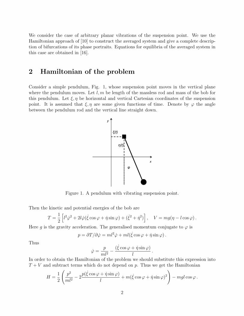
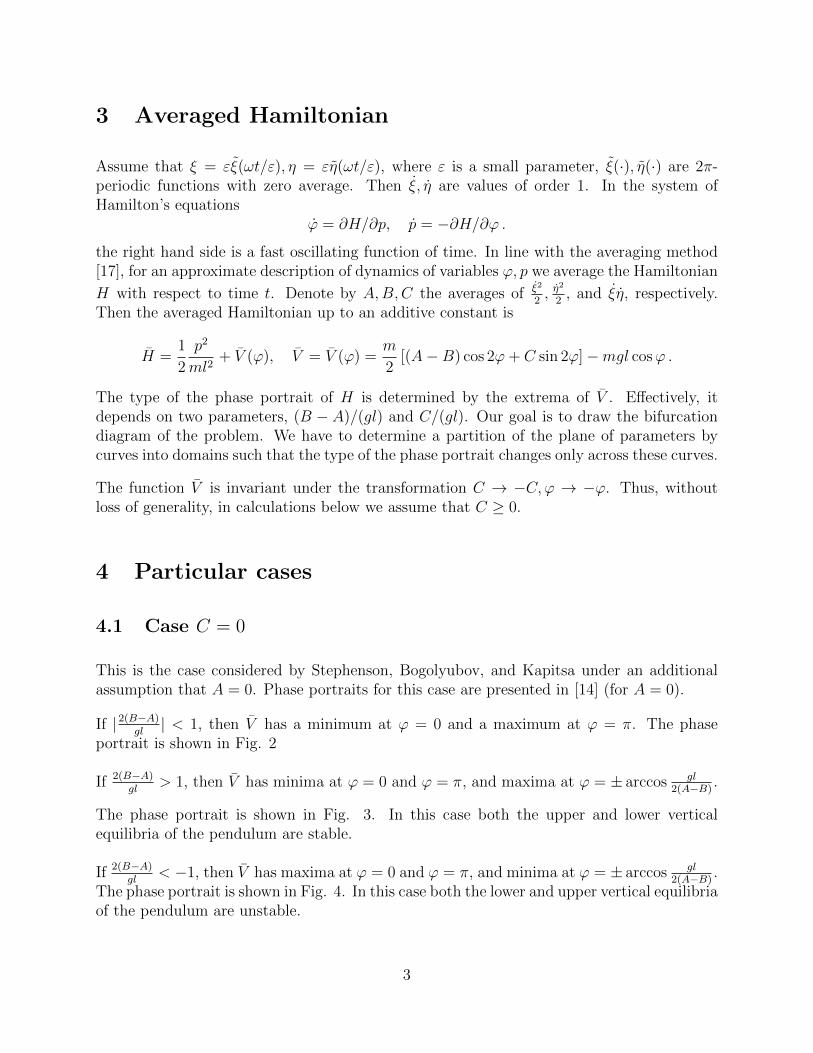
If |2(B−A)gl| < 1, then V has a minimum at ϕ = 0 and a maximum at ϕ = π. The phase

portrait is shown in Fig. 2

If 2(B−A)gl

> 1, then V has minima at ϕ = 0 and ϕ = π, and maxima at ϕ = ± arccos gl2(A−B)

.

The phase portrait is shown in Fig. 3. In this case both the upper and lower verticalequilibria of the pendulum are stable.

If 2(B−A)gl

< −1, then V has maxima at ϕ = 0 and ϕ = π, and minima at ϕ = ± arccos gl2(A−B)

.The phase portrait is shown in Fig. 4. In this case both the lower and upper vertical equilibriaof the pendulum are unstable.

3

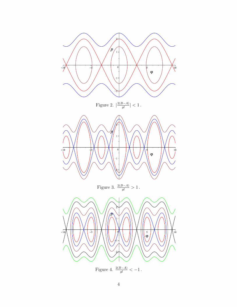
Figure 2. |2(B−A)gl| < 1 .

Figure 3. 2(B−A)gl

> 1 .

Figure 4. 2(B−A)gl

< −1 .

4

We observe a coalescence of two maxima and a minimum of the potential V at 2(B−A)gl

= 1

and that of two minima and a maximum of V at 2(B−A)gl

= −1.

4.2 Case A = B

The equation for extrema of V is

∂V /∂ϕ = m(C cos 2ϕ+ gl sinϕ) = 0

which implies

sinϕ =gl ±

√g2l2 + 8C2

4C. (1)

For the sign “−” in this formula and C > 0 the value in the right hand side is in the interval(−1, 0). Thus we have two solutions

ϕ−,1 = arcsin

(gl −

√g2l2 + 8C2

4C

), ϕ−,2 = π − ϕ−,1 .

They correspond to a minimum and a maximum of V , respectively.

If C > lg then for the sign “+” in (1) the value in the right hand side is in the interval(0, 1). In this case we have two additional solutions

ϕ+,1 = arcsin

(gl +

√g2l2 + 8C2

4C

), ϕ+,2 = π − ϕ+,1 .

They correspond to a maximum and a minimum of V , respectively.

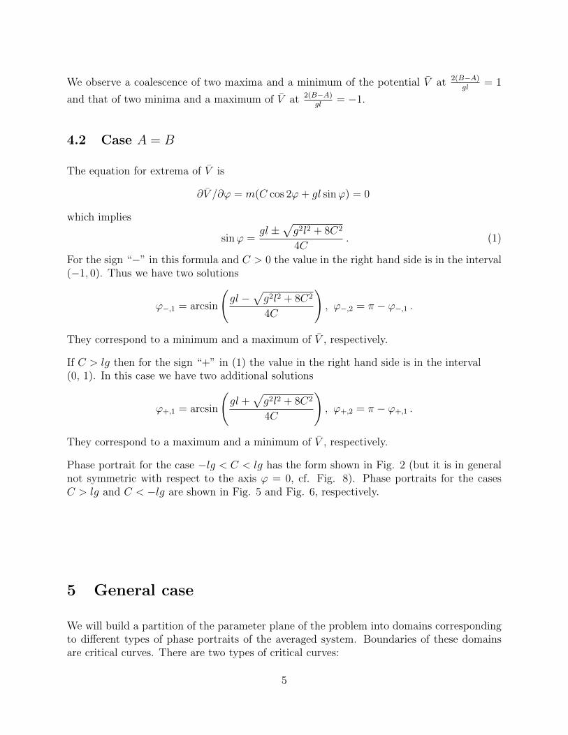
Phase portrait for the case −lg < C < lg has the form shown in Fig. 2 (but it is in generalnot symmetric with respect to the axis ϕ = 0, cf. Fig. 8). Phase portraits for the casesC > lg and C < −lg are shown in Fig. 5 and Fig. 6, respectively.

5 General case

We will build a partition of the parameter plane of the problem into domains correspondingto different types of phase portraits of the averaged system. Boundaries of these domainsare critical curves. There are two types of critical curves:

5

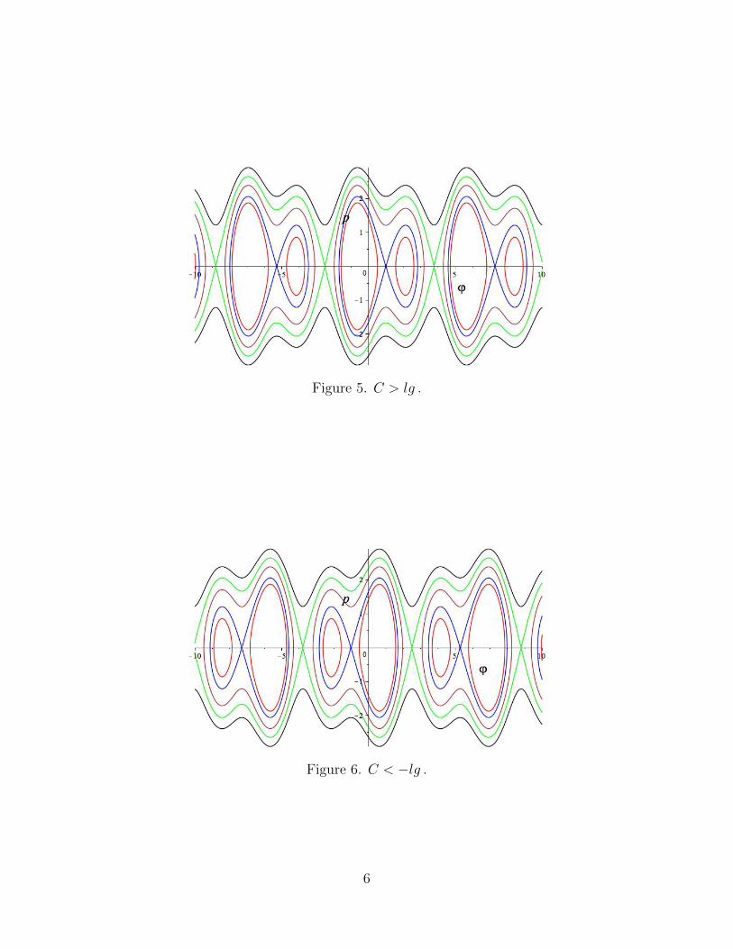
Figure 5. C > lg .

Figure 6. C < −lg .

6

• Curves corresponding to degenerate equilibria: first and second derivatives of V vanishfor parameters on these curves. The number of equilibria changes at crossing such a curvein the plane of parameters.

• Curves such that the function V has the same value at two different saddle equilibria forparameters on these curves. The number of equilibria remains the same at crossing such acurve in the plane of parameters. Curves of the second type separate adjacent regions withdifferent behavior of separatrices.

5.1 Critical curves corresponding to degenerate equilibria

These curves correspond to values of parameters such that

∂V /∂ϕ = m [(B − A) sin 2ϕ+ C cos 2ϕ+ gl sinϕ] = 0 ,

∂2V /∂ϕ2 = m [2(B − A) cos 2ϕ− 2C sin 2ϕ+ gl cosϕ] = 0

which is equivalent to

B − Agl

sin 2ϕ+C

glcos 2ϕ+ sinϕ = 0 , (2)

2(B − A)

glcos 2ϕ− 2C

glsin 2ϕ+ cosϕ = 0 .

This system is invariant with respect to the change B −A→ −(B −A), ϕ→ π − ϕ. Thus,without loss of generality, in this subsection we assume that B − A ≥ 0. As agreed earlier,we also assume that C > 0.

The system (2) can be considered as a system of two linear equations for unknown (B − A)/(gl)and C/(gl). Solving it for these unknown we get

B − Agl

= − sinϕ sin 2ϕ− 1

2cosϕ cos 2ϕ,

C

gl= − sinϕ cos 2ϕ+

1

2cosϕ sin 2ϕ .

An a bit more compact form of these relations is

B − Agl

= cos3 ϕ− 3

2cosϕ, (3)

C

gl= sin3 ϕ .

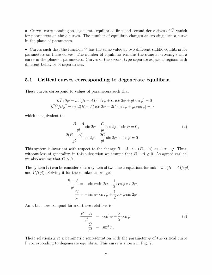
These relations give a parametric representation with the parameter ϕ of the critical curveΓ corresponding to degenerate equilibria. This curve is shown in Fig. 7.

7

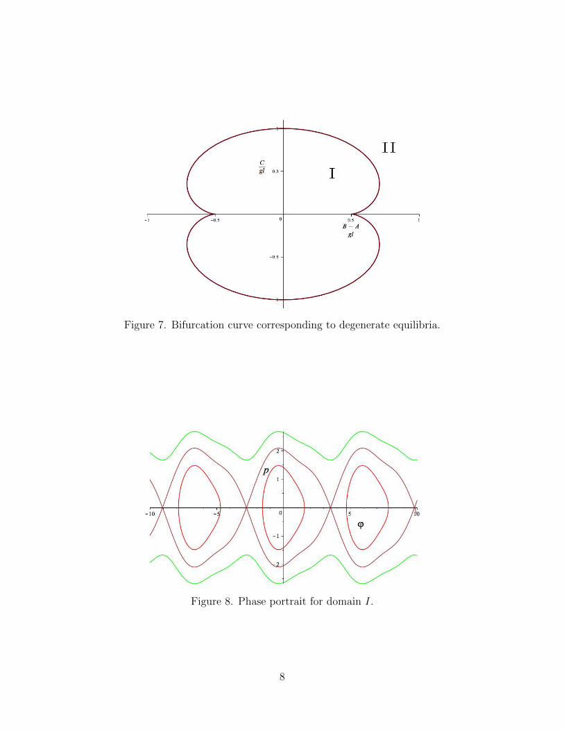
Figure 7. Bifurcation curve corresponding to degenerate equilibria.

Figure 8. Phase portrait for domain I.

8

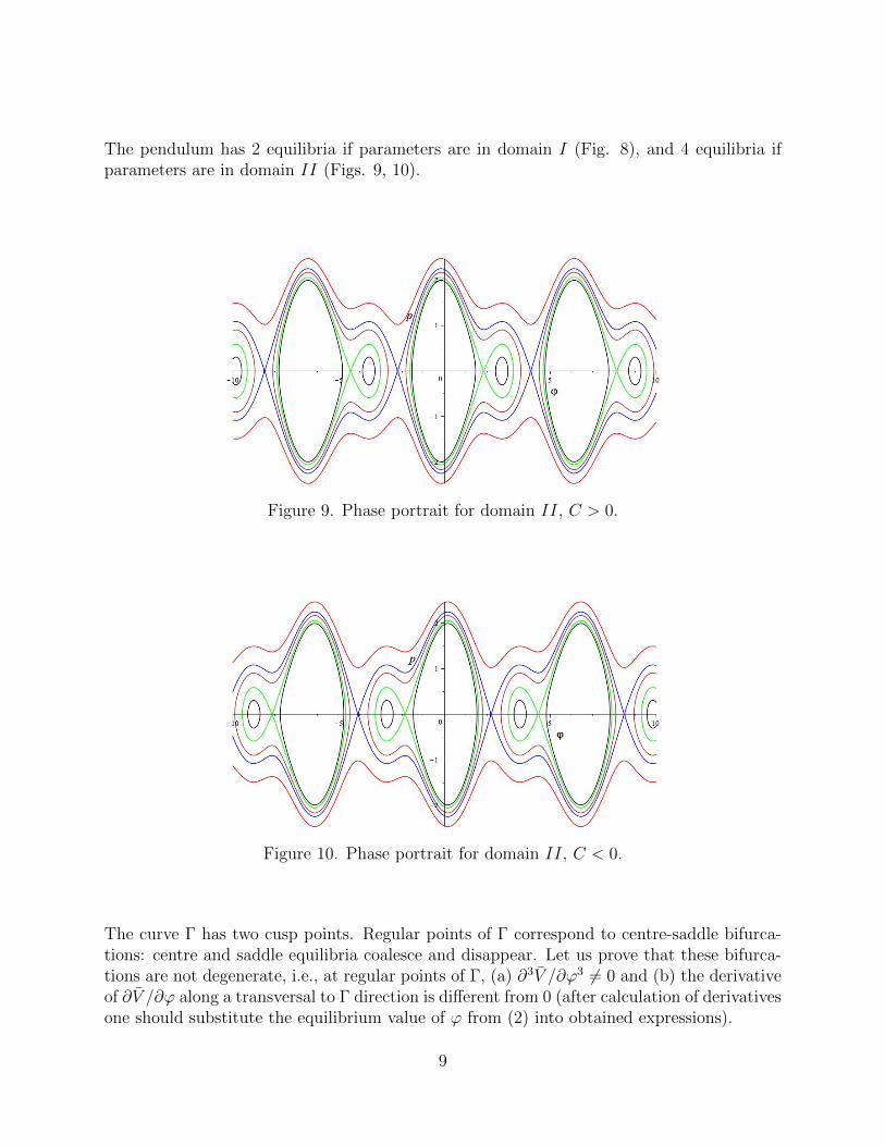
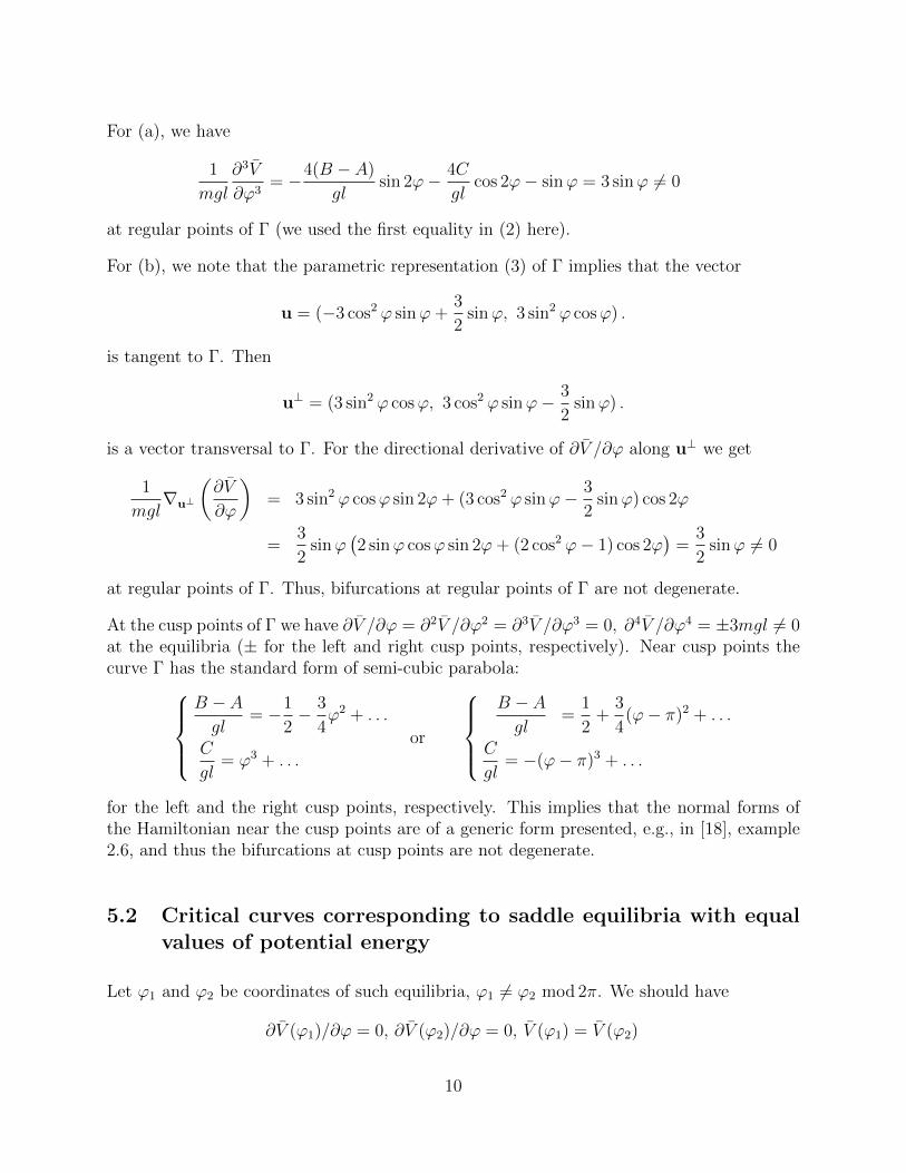
The pendulum has 2 equilibria if parameters are in domain I (Fig. 8), and 4 equilibria ifparameters are in domain II (Figs. 9, 10).

Figure 9. Phase portrait for domain II, C > 0.

Figure 10. Phase portrait for domain II, C < 0.

The curve Γ has two cusp points. Regular points of Γ correspond to centre-saddle bifurca-tions: centre and saddle equilibria coalesce and disappear. Let us prove that these bifurca-tions are not degenerate, i.e., at regular points of Γ, (a) ∂3V /∂ϕ3 6= 0 and (b) the derivativeof ∂V /∂ϕ along a transversal to Γ direction is different from 0 (after calculation of derivativesone should substitute the equilibrium value of ϕ from (2) into obtained expressions).

9

For (a), we have

1

mgl

∂3V

∂ϕ3= −4(B − A)

glsin 2ϕ− 4C

glcos 2ϕ− sinϕ = 3 sinϕ 6= 0

at regular points of Γ (we used the first equality in (2) here).

For (b), we note that the parametric representation (3) of Γ implies that the vector

u = (−3 cos2 ϕ sinϕ+3

2sinϕ, 3 sin2 ϕ cosϕ) .

is tangent to Γ. Then

u⊥ = (3 sin2 ϕ cosϕ, 3 cos2 ϕ sinϕ− 3

2sinϕ) .

is a vector transversal to Γ. For the directional derivative of ∂V /∂ϕ along u⊥ we get

1

mgl∇u⊥

(∂V

∂ϕ

)= 3 sin2 ϕ cosϕ sin 2ϕ+ (3 cos2 ϕ sinϕ− 3

2sinϕ) cos 2ϕ

=3

2sinϕ

(2 sinϕ cosϕ sin 2ϕ+ (2 cos2 ϕ− 1) cos 2ϕ

)=

3

2sinϕ 6= 0

at regular points of Γ. Thus, bifurcations at regular points of Γ are not degenerate.

At the cusp points of Γ we have ∂V /∂ϕ = ∂2V /∂ϕ2 = ∂3V /∂ϕ3 = 0, ∂4V /∂ϕ4 = ±3mgl 6= 0at the equilibria (± for the left and right cusp points, respectively). Near cusp points thecurve Γ has the standard form of semi-cubic parabola:

B − Agl

= −1

2− 3

4ϕ2 + . . .

C

gl= ϕ3 + . . .

or

B − Agl

=1

2+

3

4(ϕ− π)2 + . . .

C

gl= −(ϕ− π)3 + . . .

for the left and the right cusp points, respectively. This implies that the normal forms ofthe Hamiltonian near the cusp points are of a generic form presented, e.g., in [18], example2.6, and thus the bifurcations at cusp points are not degenerate.

5.2 Critical curves corresponding to saddle equilibria with equalvalues of potential energy

Let ϕ1 and ϕ2 be coordinates of such equilibria, ϕ1 6= ϕ2 mod 2π. We should have

∂V (ϕ1)/∂ϕ = 0, ∂V (ϕ2)/∂ϕ = 0, V (ϕ1) = V (ϕ2)

10

or, in the explicit form,

B − Agl

sin 2ϕ1 +C

glcos 2ϕ1 + sinϕ1 = 0 , (4)

B − Agl

sin 2ϕ2 +C

glcos 2ϕ2 + sinϕ2 = 0 ,

−B − Agl

(cos 2ϕ1 − cos 2ϕ2) +C

gl(sin 2ϕ1 − sin 2ϕ2)− 2(cosϕ1 − cosϕ2) = 0 .

As ϕ1 6= ϕ2 mod 2π, we can divide the last equation by 4 sin ϕ1−ϕ2

2. It reduces to

B − Agl

sin(ϕ1 + ϕ2) cosϕ1 − ϕ2

2+C

glcos

ϕ1 − ϕ2

2cos(ϕ1 + ϕ2) + sin

ϕ1 + ϕ2

2= 0 . (5)

The first two equations in (4) can be considered as a system of two linear equations forunknown (B − A)/(gl) and C/(gl). The determinant of this system is

D = sin 2(ϕ1 − ϕ2) .

We should consider two cases: D = 0 and D 6= 0.

In the case D 6= 0 we solve first two equations in (4) for (B − A)/(gl) and C/(gl) and get

B − Agl

=− sinϕ1 cos 2ϕ2 + sinϕ2 cos 2ϕ1

sin 2(ϕ1 − ϕ2),

C

gl=

sinϕ1 sin 2ϕ2 − sinϕ2 sin 2ϕ1

sin 2(ϕ1 − ϕ2).

These relations can be rewritten in the form

B − Agl

=2 sin ϕ1−ϕ2

2cos ϕ1+ϕ2

2(cos(ϕ1 + ϕ2)− cos(ϕ1 − ϕ2)− 1)

sin 2(ϕ1 − ϕ2),

C

gl=

2 sin ϕ1−ϕ2

2sin ϕ1+ϕ2

2(− cos(ϕ1 + ϕ2) + cos(ϕ1 − ϕ2))

sin 2(ϕ1 − ϕ2)

or, after a cancellation, in the form

B − Agl

=cos ϕ1+ϕ2

2(cos(ϕ1 + ϕ2)− cos(ϕ1 − ϕ2)− 1)

2 cos(ϕ1 − ϕ2) cos ϕ1−ϕ2

2

,

C

gl=

sin ϕ1+ϕ2

2(− cos(ϕ1 + ϕ2) + cos(ϕ1 − ϕ2))

2 cos(ϕ1 − ϕ2) cos ϕ1−ϕ2

2

.

Now we substitute these relations into equation (5), and, assuming that ϕ1 6= −ϕ2 mod 2π,divide the obtained equation by sin ϕ1+ϕ2

2. We get

cos2 ϕ1+ϕ2

2(cos(ϕ1 + ϕ2)− cos(ϕ1 − ϕ2)− 1)

cos(ϕ1 − ϕ2)

+(− cos(ϕ1 + ϕ2) + cos(ϕ1 − ϕ2))

2 cos(ϕ1 − ϕ2)cos(ϕ1 + ϕ2) + 1 = 0

11

which is equivalent to

(1 + cos(ϕ1 + ϕ2)) (cos(ϕ1 + ϕ2)− cos(ϕ1 − ϕ2)− 1)

+ (− cos(ϕ1 + ϕ2) + cos(ϕ1 − ϕ2)) cos(ϕ1 + ϕ2) + 2 cos(ϕ1 − ϕ2) = 0

and then equivalent tocos(ϕ1 − ϕ2) = 1

which can not be satisfied for ϕ1 6= ϕ2 mod 2π.

Thus, the only remaining possibilities are related to the special cases D = sin 2(ϕ1−ϕ2) = 0and ϕ1 = −ϕ2 mod 2π. It is easy to check that each of these relations together with relations(4) implies C = 0. As ϕ1 and ϕ2 should correspond to different saddles, we should considerthe domain were there are four equilibria. Thus, possible bifurcational curves are rays{C = 0, 2(B−A)

gl> 1} and {C = 0, 2(B−A)

gl< −1}. The equilibria with equal values of potential

energy are saddles for the first and centres for the second of these rays (see Figs. 3 and 4).

Thus the only bifurcational curve of the considered type is the ray {C = 0, 2(B−A)gl

> 1}.

5.3 Bifurcation diagram

The partition of the plane of parameters into domains with qualitatively different phaseportraits is shown in Fig. 11. The pendulum has 2 equilibria if parameters are in domain I(phase portrait in Fig. 8), and 4 equilibria if parameters are in domain II (phase portraitin Fig. 9 for C > 0 and Fig. 10 for C < 0; these phase portraits are topologically thesame but have different types of asymmetry of the eight-shaped separatrix). The boundary

Γ between these domains is the curve of degenerate equilibria. The ray {C = 0, 2(B−A)gl

> 1}corresponds to phase portraits with a heteroclinic trajectory (Fig. 3). Passage through thisray transforms the phase portrait of Fig. 9 via that of Fig. 3 to that of Fig. 10. At approachthe curve of degenerate equilibria from the domain II at C > 0 (respectively C < 0), theright (respectively, the left) loop of eight-shaped separatrix shrinks to a point and disappears.

6 Conclusion

Our study in this paper provides a complete description of bifurcations of phase portraits fora pendulum with vibrating suspension point in the approximation of the averaging method.The relation of such a description to dynamics in the exact (not averaged) problem forhigh-frequency oscillations is discussed, e.g., in [15], Sect. 6.3.3.B. One should consider thePoincare return map for the plane ϕ, p (Poincare section t = 0 mod 2πε

ω). Fixed points of this

12

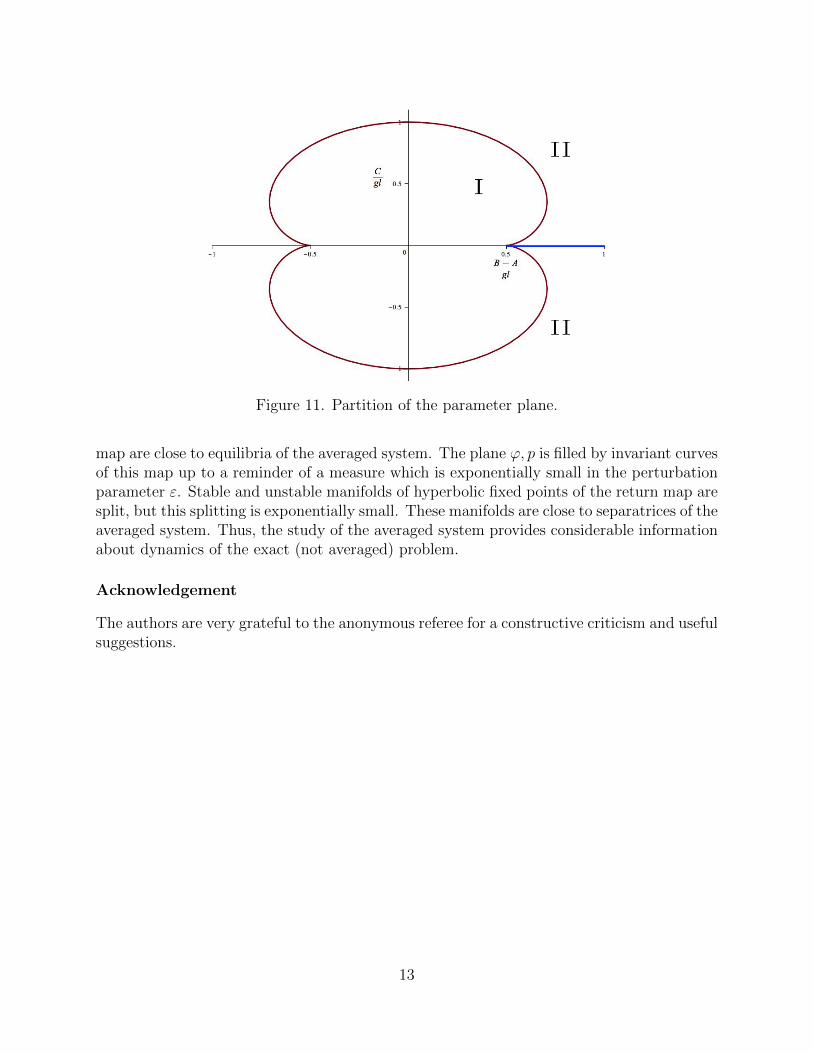
Figure 11. Partition of the parameter plane.

map are close to equilibria of the averaged system. The plane ϕ, p is filled by invariant curvesof this map up to a reminder of a measure which is exponentially small in the perturbationparameter ε. Stable and unstable manifolds of hyperbolic fixed points of the return map aresplit, but this splitting is exponentially small. These manifolds are close to separatrices of theaveraged system. Thus, the study of the averaged system provides considerable informationabout dynamics of the exact (not averaged) problem.

Acknowledgement

The authors are very grateful to the anonymous referee for a constructive criticism and usefulsuggestions.

13

References

[1] Stephenson A. On induced stability. Philosophical Magazine Series 6 1908; 15: 233-6.

[2] Stephenson A. On a new type of dynamical stability. Mem Proc Manch Lit Phil Soc 1908;52 (8): 1-10.

[3] Bogolyubov NN. Perturbation theory in nonlinear mechanics. In: Collection of papers of InstConstuct Mekh Akad Nauk UkrSSR 1950; 14: 9-34 (in Russian).

[4] Kapitsa PL. Dynamic stability of a pendulum with oscillating point of suspension. Sov.Phys. JETP 1951; 21: 588-597 (in Russian), see also Collected papers of P. L. Kapitza, vol.2, 714-725. London: Pergamon; 1965.

[5] Kapitsa PL. A pendulum with vibrating point of suspension. Usp Phys Nauk 1951; 44: 7-20(in Russian).

[6] Landau LD, Lifshitz EM. Course of theoretical physics, Vol. 1: Mechanics. Oxford: Perga-mon; 1988.

[7] Levi M. Geometry of Kapitsa’s potential. Nonlinearity 1998; 11: 1365-8.

[8] Bardin BS, Markeyev AP. On the stability of equilibrium of a pendulum with vertical oscil-lations of its suspension point. J Appl Math Mech 1995; 59: 879-86.

[9] Ovseyevich AI. The stability of an inverted pendulum when there are rapid random oscilla-tions of the suspension point. J Appl Math Mech 2006; 70: 761-8.

[10] Burd VSh, Matveev VN. Asymptotic methods on an infinite interval in problems of nonlinearmechanics. Yaroslavl’: Yaroslavl’ Univ; 1985 (in Russian).

[11] Stephenson A. On induced stability. Philosophical Magazine Series 6 1909; 17: 765-6.

[12] Acheson D. A pendulum theorem. Proc R Soc London 1993; 433: 239-45.

[13] Kholostova O. On the motions of a double pendulum with vibrating suspension point. Me-chanics of Solids 2009; 44: 184-97.

[14] Treschev D. Some aspects of finite-dimensional Hamiltonian dynamics. In: Craig W (editor).Hamiltonian dynamical systems and applications, 1-19. Dordrecht: Springer; 2008.

[15] Arnold VI, Kozlov VV, Neishtadt AI. Mathematical aspects of classical and celestial me-chanics. Berlin: Springer; 2006.

[16] Akulenko LD. Asymptotic analysis of dynamical systems subjected to high-frequency inter-actions. J Appl Math Mech. 1994; 58(3): 393-402.

[17] Bogoliubov NN, Mitropolsky YA. Asymptotic methods in the theory of non-linear oscilla-tions. New York: Gordon and Breach Sci Publ; 1961.

[18] Hanßmann H. Local and semi-local bifurcations in Hamiltonian systems - Results and ex-amples. Lecture Notes in Mathematics 1893. Berlin: Springer; 2007.

14