IMT Institute for Advanced Studies

Lucca, Italy

Big Data and the Web: Algorithms forData Intensive Scalable Computing

PhD Program in Computer Science and Engineering

XXIV Cycle

By

Gianmarco De Francisci Morales

2012

The dissertation of Gianmarco De Francisci Morales isapproved.

Program Coordinator: Prof. Rocco De Nicola, IMT Lucca

Supervisor: Dott. Claudio Lucchese, ISTI-CNR Pisa

Co-Supervisor: Dott. Ranieri Baraglia, ISTI-CNR Pisa

Tutor: Dott. Leonardo Badia, University of Padova

The dissertation of Gianmarco De Francisci Morales has been reviewedby:

Aristides Gionis, Yahoo! Research Barcelona

Iadh Ounis, University of Glasgow

IMT Institute for Advanced Studies, Lucca

2012

Where is the wisdom wehave lost in knowledge?Where is the knowledge wehave lost in information?

To my mother, for her unconditional love

and support throughout all these years.

Acknowledgements

I owe my deepest and earnest gratitude to my supervisor,Claudio Lucchese, who shepherded me towards this goal withgreat wisdom and everlasting patience.

I am grateful to all my co-authors, without whom this workwould have been impossible. A separate acknowledgementgoes to Aris Gionis for his precious advice, constant presenceand exemplary guidance.

I thank all the friends and colleagues in Lucca with whomI shared the experience of being a Ph.D. student, my Lab inPisa that accompanied me through this journey, and all thepeople in Barcelona that helped me feel like at home.

Thanks to my family and to everyone who believed in me.

ix

Contents

List of Figures xiii

List of Tables xv

Publications xvi

Abstract xviii

1 Introduction 11.1 The Data Deluge . . . . . . . . . . . . . . . . . . . . . . . . 2

1.2 Mining the Web . . . . . . . . . . . . . . . . . . . . . . . . . 6

1.2.1 Taxonomy of Web data . . . . . . . . . . . . . . . . . 8

1.3 Management of Data . . . . . . . . . . . . . . . . . . . . . . 10

1.3.1 Parallelism . . . . . . . . . . . . . . . . . . . . . . . . 11

1.3.2 Data Intensive Scalable Computing . . . . . . . . . 14

1.4 Contributions . . . . . . . . . . . . . . . . . . . . . . . . . . 16

2 Related Work 192.1 DISC systems . . . . . . . . . . . . . . . . . . . . . . . . . . 20

2.2 MapReduce . . . . . . . . . . . . . . . . . . . . . . . . . . . 24

2.2.1 Computational Models and Extensions . . . . . . . 27

2.3 Streaming . . . . . . . . . . . . . . . . . . . . . . . . . . . . 30

2.3.1 S4 . . . . . . . . . . . . . . . . . . . . . . . . . . . . . 31

2.4 Algorithms . . . . . . . . . . . . . . . . . . . . . . . . . . . . 34

x

3 SSJ 373.1 Introduction . . . . . . . . . . . . . . . . . . . . . . . . . . . 383.2 Problem definition and preliminaries . . . . . . . . . . . . . 403.3 Related work . . . . . . . . . . . . . . . . . . . . . . . . . . . 42

3.3.1 MapReduce Term-Filtering (ELSA) . . . . . . . . . . 423.3.2 MapReduce Prefix-Filtering (VERN) . . . . . . . . . 44

3.4 SSJ Algorithms . . . . . . . . . . . . . . . . . . . . . . . . . 463.4.1 Double-Pass MapReduce Prefix-Filtering (SSJ-2) . . 463.4.2 Double-Pass MapReduce Prefix-Filtering with Re-

mainder File (SSJ-2R) . . . . . . . . . . . . . . . . . 493.4.3 Partitioning . . . . . . . . . . . . . . . . . . . . . . . 52

3.5 Complexity analysis . . . . . . . . . . . . . . . . . . . . . . 533.6 Experimental evaluation . . . . . . . . . . . . . . . . . . . . 56

3.6.1 Running time . . . . . . . . . . . . . . . . . . . . . . 573.6.2 Map phase . . . . . . . . . . . . . . . . . . . . . . . . 593.6.3 Shuffle size . . . . . . . . . . . . . . . . . . . . . . . 623.6.4 Reduce phase . . . . . . . . . . . . . . . . . . . . . . 633.6.5 Partitioning the remainder file . . . . . . . . . . . . 65

3.7 Conclusions . . . . . . . . . . . . . . . . . . . . . . . . . . . 66

4 SCM 674.1 Introduction . . . . . . . . . . . . . . . . . . . . . . . . . . . 684.2 Related work . . . . . . . . . . . . . . . . . . . . . . . . . . . 714.3 Problem definition . . . . . . . . . . . . . . . . . . . . . . . 714.4 Application scenarios . . . . . . . . . . . . . . . . . . . . . . 724.5 Algorithms . . . . . . . . . . . . . . . . . . . . . . . . . . . . 74

4.5.1 Computing the set of candidate edges . . . . . . . . 744.5.2 The STACKMR algorithm . . . . . . . . . . . . . . . 754.5.3 Adaptation in MapReduce . . . . . . . . . . . . . . 814.5.4 The GREEDYMR algorithm . . . . . . . . . . . . . . 844.5.5 Analysis of the GREEDYMR algorithm . . . . . . . . 85

4.6 Experimental evaluation . . . . . . . . . . . . . . . . . . . . 874.7 Conclusions . . . . . . . . . . . . . . . . . . . . . . . . . . . 97

xi

5 T.Rex 985.1 Introduction . . . . . . . . . . . . . . . . . . . . . . . . . . . 995.2 Related work . . . . . . . . . . . . . . . . . . . . . . . . . . . 1045.3 Problem definition and model . . . . . . . . . . . . . . . . . 106

5.3.1 Entity popularity . . . . . . . . . . . . . . . . . . . . 1135.4 System overview . . . . . . . . . . . . . . . . . . . . . . . . 1165.5 Learning algorithm . . . . . . . . . . . . . . . . . . . . . . . 119

5.5.1 Constraint selection . . . . . . . . . . . . . . . . . . 1215.5.2 Additional features . . . . . . . . . . . . . . . . . . . 122

5.6 Experimental evaluation . . . . . . . . . . . . . . . . . . . . 1235.6.1 Datasets . . . . . . . . . . . . . . . . . . . . . . . . . 1235.6.2 Test set . . . . . . . . . . . . . . . . . . . . . . . . . . 1255.6.3 Evaluation measures . . . . . . . . . . . . . . . . . . 1265.6.4 Baselines . . . . . . . . . . . . . . . . . . . . . . . . . 1285.6.5 Results . . . . . . . . . . . . . . . . . . . . . . . . . . 128

5.7 Conclusions . . . . . . . . . . . . . . . . . . . . . . . . . . . 130

6 Conclusions 131

A List of Acronyms 135

References 137

xii

List of Figures

1.1 The petabyte age. . . . . . . . . . . . . . . . . . . . . . . . . 31.2 Data Information Knowledge Wisdom hierarchy. . . . . . . 41.3 Complexity of contributed algorithms. . . . . . . . . . . . . 17

2.1 DISC architecture. . . . . . . . . . . . . . . . . . . . . . . . . 202.2 Data flow in the MapReduce programming paradigm. . . . 262.3 Overview of S4. . . . . . . . . . . . . . . . . . . . . . . . . . 322.4 Twitter hashtag counting in S4. . . . . . . . . . . . . . . . . 33

3.1 ELSA example. . . . . . . . . . . . . . . . . . . . . . . . . . . 443.2 VERN example. . . . . . . . . . . . . . . . . . . . . . . . . . 463.3 Pruned document pair: the left part (orange/light) has

been pruned, the right part (blue/dark) has been indexed. 473.4 SSJ-2 example. . . . . . . . . . . . . . . . . . . . . . . . . . 483.5 SSJ-2R example. . . . . . . . . . . . . . . . . . . . . . . . . . 533.6 Running time. . . . . . . . . . . . . . . . . . . . . . . . . . . 583.7 Average mapper completion time. . . . . . . . . . . . . . . 593.8 Mapper completion time distribution. . . . . . . . . . . . . 603.9 Effect of Prefix-filtering on inverted list length distribution. 623.10 Shuffle size. . . . . . . . . . . . . . . . . . . . . . . . . . . . 633.11 Average reducer completion time. . . . . . . . . . . . . . . 643.12 Remainder file and shuffle size varying K. . . . . . . . . . . 65

4.1 Example of a STACKMR run. . . . . . . . . . . . . . . . . . 80

xiii

4.2 Communication pattern for iterative graph algorithms onMR. . . . . . . . . . . . . . . . . . . . . . . . . . . . . . . . . 83

4.3 Distribution of edge similarities for the datasets. . . . . . . 884.4 Distribution of capacities for the three datasets. . . . . . . . 894.5 flickr-small dataset: matching value and number of

iterations as a function of the number of edges. . . . . . . . 924.6 flickr-large dataset: matching value and number of

iterations as a function of the number of edges. . . . . . . . 934.7 yahoo-answers dataset: matching value and number of

iterations as a function of the number of edges. . . . . . . . 944.8 Violation of capacities for STACKMR. . . . . . . . . . . . . . 954.9 Normalized value of the b-matching achieved by the GREEDY-

MR algorithm as a function of the number of MapReduceiterations. . . . . . . . . . . . . . . . . . . . . . . . . . . . . . 96

5.1 Osama Bin Laden trends on Twitter and news streams. . . . 1015.2 Joplin tornado trends on Twitter and news streams. . . . . . 1025.3 Cumulative Osama Bin Laden trends (news, Twitter and

clicks). . . . . . . . . . . . . . . . . . . . . . . . . . . . . . . 1135.4 News-click delay distribution. . . . . . . . . . . . . . . . . . 1145.5 Cumulative news-click delay distribution. . . . . . . . . . . 1155.6 Overview of the T.REX system. . . . . . . . . . . . . . . . . 1175.7 T.REX news ranking dataflow. . . . . . . . . . . . . . . . . . 1195.8 Distribution of entities in Twitter. . . . . . . . . . . . . . . . 1235.9 Distribution of entities in news. . . . . . . . . . . . . . . . . 1245.10 Average discounted cumulated gain on related entities. . . 129

xiv

List of Tables

2.1 Major Data Intensive Scalable Computing (DISC) systems. 21

3.1 Symbols and quantities. . . . . . . . . . . . . . . . . . . . . 543.2 Complexity analysis. . . . . . . . . . . . . . . . . . . . . . . 543.3 Samples from the TREC WT10G collection. . . . . . . . . . 573.4 Statistics for the four algorithms on the three datasets. . . . 61

4.1 Dataset characteristics. |T |: number of items; |C|: numberof users; |E|: total number of item-user pairs with non zerosimilarity. . . . . . . . . . . . . . . . . . . . . . . . . . . . . . 91

5.1 Table of symbols. . . . . . . . . . . . . . . . . . . . . . . . . 1075.2 MRR, precision and coverage. . . . . . . . . . . . . . . . . . 128

xv

Publications

1. G. De Francisci Morales, A. Gionis, C. Lucchese, “From Chatter to Head-lines: Harnessing the Real-Time Web for Personalized News Recommen-dations", WSDM’12, 5th ACM International Conference on Web Searchand Data Mining, Seattle, 2012, pp. 153-162.

2. G. De Francisci Morales, A. Gionis, M. Sozio, “Social Content Matching inMapReduce”, PVLDB, Proceedings of the VLDB Endowment, 4(7):460-469,2011.

3. R. Baraglia, G. De Francisci Morales, C. Lucchese, “Document SimilaritySelf-Join with MapReduce”, ICDM’10, 10th IEEE International Conferenceon Data Mining, Sydney, 2010, pp. 731-736.

4. G. De Francisci Morales, C. Lucchese, R. Baraglia, “Scaling Out All PairsSimilarity Search with MapReduce”, LSDS-IR’10, 8th Workshop on Large-Scale Distributed Systems for Information Retrieval, @SIGIR’10, Geneva,2010, pp. 25-30.

5. G. De Francisci Morales, C. Lucchese, R. Baraglia, “Large-scale Data Anal-ysis on the Cloud”, XXIV Convegno Annuale del CMG-Italia, Roma, 2010.

xvi

Presentations

1. G. De Francisci Morales, “Harnessing the Real-Time Web for PersonalizedNews Recommendation”, Yahoo! Labs, Sunnyvale, 16 Februrary 2012.

2. G. De Francisci Morales, “Big Data and the Web: Algorithms for Data In-tensive Scalable Computing”, WSDM’12, Seattle, 8 Februrary 2012.

3. G. De Francisci Morales, “Social Content Matching in MapReduce”, Yahoo!Research, Barcelona, 10 March 2011.

4. G. De Francisci Morales, “Cloud Computing for Large Scale Data Analy-sis”, Yahoo! Research, Barcelona, 2 December 2010.

5. G. De Francisci Morales, “Scaling Out All Pairs Similarity Search withMapReduce”, Summer School on Social Networks, Lipari, 6 July 2010.

6. G. De Francisci Morales, “How to Survive the Data Deluge: Petabyte ScaleCloud Computing”, ISTI-CNR, Pisa, 18 January 2010.

xvii

Abstract

This thesis explores the problem of large scale Web miningby using Data Intensive Scalable Computing (DISC) systems.Web mining aims to extract useful information and modelsfrom data on the Web, the largest repository ever created.DISC systems are an emerging technology for processing hugedatasets in parallel on large computer clusters.

Challenges arise from both themes of research. The Web isheterogeneous: data lives in various formats that are bestmodeled in different ways. Effectively extracting informationrequires careful design of algorithms for specific categories ofdata. The Web is huge, but DISC systems offer a platform forbuilding scalable solutions. However, they provide restrictedcomputing primitives for the sake of performance. Efficientlyharnessing the power of parallelism offered by DISC systemsinvolves rethinking traditional algorithms.

This thesis tackles three classical problems in Web mining.First we propose a novel solution to finding similar items ina bag of Web pages. Second we consider how to effectivelydistribute content from Web 2.0 to users via graph matching.Third we show how to harness the streams from the real-timeWeb to suggest news articles. Our main contribution lies inrethinking these problems in the context of massive scale Webmining, and in designing efficient MapReduce and streamingalgorithms to solve these problems on DISC systems.

xviii

Chapter 1

Introduction

An incredible “data deluge” is currently drowning the world. Data sourcesare everywhere, from Web 2.0 and user-generated content to large scien-tific experiments, from social networks to wireless sensor networks. Thismassive amount of data is a valuable asset in our information society.

Data analysis is the process of inspecting data in order to extractuseful information. Decision makers commonly use this information todrive their choices. The quality of the information extracted by this pro-cess greatly benefits from the availability of extensive datasets.

The Web is the biggest and fastest growing data repository in theworld. Its size and diversity make it the ideal resource to mine for usefulinformation. Data on the Web is very diverse in both content and format.Consequently, algorithms for Web mining need to take into account thespecific characteristics of the data to be efficient.

As we enter the “petabyte age”, traditional approaches for data analy-sis begin to show their limits. Commonly available data analysis tools areunable to keep up with the increase in size, diversity and rate of changeof the Web. Data Intensive Scalable Computing is an emerging alterna-tive technology for large scale data analysis. DISC systems combine bothstorage and computing in a distributed and virtualized manner. Thesesystems are built to scale to thousands of computers, and focus on faulttolerance, cost effectiveness and ease of use.

1

1.1 The Data Deluge

How would you sort 1GB of data? Today’s computers have enoughmemory to keep this quantity of data, so any optimal in-memory al-gorithm will suffice. What if you had to sort 100 GB of data? Even ifsystems with more than 100 GB of memory exist, they are by no meanscommon or cheap. So the best solution is to use a disk based sorting al-gorithm. However, what if you had 10 TB of data to sort? At a transferrate of about 100 MB/s for a normal disk it would take more than oneday to make a single pass over the dataset. In this case the bandwidthbetween memory and disk is the bottleneck. In any case, today’s disksare usually 1 to 2 TB in size, which means that just to hold the data weneed multiple disks. In order to obtain acceptable completion times, wealso need to use multiple computers and a parallel algorithm.

This example illustrates a general point: the same problem at differ-ent scales needs radically different solutions. In many cases we evenneed change the model we use to reason about the problem becausethe simplifying assumptions made by the models do not hold at everyscale. Citing Box and Draper (1986) “Essentially, all models are wrong,but some are useful”, and arguably “most of them do not scale”.

Currently, an incredible “data deluge” is drowning the world. Theamount of data we need to sift through every day is enormous. For in-stance the results of a search engine query are so many that we are notable to examine all of them, and indeed the competition now focuses thetop ten results. This is just an example of a more general trend.

The issues raised by large datasets in the context of analytical ap-plications are becoming ever more important as we enter the so-called“petabyte age”. Figure 1.1 shows the sizes of the datasets for problemswe currently face (Anderson, 2008). The datasets are orders of magni-tude greater than what fits on a single hard drive, and their managementposes a serious challenge. Web companies are currently facing this issue,and striving to find efficient solutions. The ability to manage and ana-lyze more data is a distinct competitive advantage for them. This issuehas been labeled in various ways: petabyte scale, Web scale or “big data”.

2

Figure 1.1: The petabyte age.

But how do we define “big data”? The definition is of course relativeand evolves in time as technology progresses. Indeed, thirty years agoone terabyte would be considered enormous, while today we are com-monly dealing with such quantity of data.

Gartner (2011) puts the focus not only on size but on three differentdimensions of growth for data, the 3V: Volume, Variety and Velocity. Thedata is surely growing in size, but also in complexity as it shows up indifferent formats and from different sources that are hard to integrate,and in dynamicity as it arrives continuously, changes rapidly and needsto be processed as fast as possible.

Loukides (2010) offers a different point of view by saying that bigdata is “when the size of the data itself becomes part of the problem”and “traditional techniques for working with data run out of steam”.

Along the same lines, Jacobs (2009) states that big data is “data whosesize forces us to look beyond the tried-and-true methods that are preva-lent at that time”. This means that we can call big an amount of data thatforces us to use or create innovative methodologies.

We can think that the intrinsic characteristics of the object to be an-alyzed demand modifications to traditional data managing procedures.

3

Understanding

Connectedness

Data

Knowledge

Wisdom

InformationUnd

erstand

Relatio

ns

Understand

Pattern

s

Understand

Principles

Figure 1.2: Data Information Knowledge Wisdom hierarchy.

Alternatively, we can take the point of view of the subject who needs tomanage the data. The emphasis is thus on user requirements such asthroughput and latency. In either case, all the previous definitions hintto the fact that big data is a driver for research.

But why are we interested in data? It is common belief that data with-out a model is just noise. Models are used to describe salient features inthe data, which can be extracted via data mining. Figure 1.2 depicts thepopular Data Information Knowledge Wisdom (DIKW) hierarchy (Row-ley, 2007). In this hierarchy data stands at the lowest level and bearsthe smallest level of understanding. Data needs to be processed and con-densed into more connected forms in order to be useful for event com-prehension and decision making. Information, knowledge and wisdomare these forms of understanding. Relations and patterns that allow togain deeper awareness of the process that generated the data, and prin-ciples that can guide future decisions.

4

For data mining, the scaling up of datasets is a “double edged” sword.On the one hand, it is an opportunity because “no data is like more data”.Deeper insights are possible when more data is available (Halevy et al.,2009). Oh the other hand, it is a challenge. Current methodologies areoften not suitable to handle huge datasets, so new solutions are needed.

The large availability of data potentially enables more powerful anal-ysis and unexpected outcomes. For example, Google Flu Trends candetect regional flu outbreaks up to ten days faster than the Center forDisease Control and Prevention by analyzing the volume of flu-relatedqueries to the Web search engine (Ginsberg et al., 2008). Companies likeIBM and Google are using large scale data to solve extremely challeng-ing problems like avoiding traffic congestion, designing self-driving carsor understanding Jeopardy riddles (Loukides, 2011). Chapter 2 presentsmore examples of interesting large scale data analysis problems.

Data originates from a wide variety sources. Radio-Frequency Iden-tification (RFID) tags and Global Positioning System (GPS) receivers arealready spread all around us. Sensors like these produce petabytes ofdata just as a result of their sheer numbers, thus starting the so called“industrial revolution of data” (Hellerstein, 2008).

Scientific experiments are also a huge data source. The Large HadronCollider at CERN is expected to generate around 50 TB of raw data perday. The Hubble telescope captured millions of astronomical images,each weighting hundreds of megabytes. Computational biology experi-ments like high-throughput genome sequencing produce large quantitiesof data that require extensive post-processing.

The focus of our work is directed to another massive source of data:the Web. The importance of the Web from the scientific, economical andpolitical point of view has grown dramatically over the last ten years, somuch that internet access has been declared a human right by the UnitedNations (La Rue, 2011). Web users produce vast amounts of text, audioand video contents in the Web 2.0. Relationships and tags in social net-works create massive graphs spanning millions of vertexes and billionsof edges. In the next section we highlight some of the opportunities andchallenges found when mining the Web.

5

1.2 Mining the Web

The Web is easily the single largest publicly accessible data source in theworld (Liu, 2007). The continuous usage of the Web has accelerated itsgrowth. People and companies keep adding to the already enormousmass of pages already present.

In the last decade the Web has increased its importance to the point ofbecoming the center of our digital lives (Hammersley, 2011). People shopand read news on the Web, governments offer public services through itand enterprises develop Web marketing strategies. Investments in Webadvertising have surpassed the ones in television and newspaper in mostcountries. This is a clear testament to the importance of the Web.

The estimated size of the indexable Web was at least 11.5 billion pagesas of January 2005 (Gulli and Signorini, 2005). Today, the Web size isestimated between 50 and 100 billion pages and roughly doubling everyeight months (Baeza-Yates and Ribeiro-Neto, 2011), faster than Moore’slaw. Furthermore, the Web has become infinite for practical purpose, as itis possible to generate an infinite number of dynamic pages. As a result,there is on the Web an abundance of data with growing value.

The value of this data lies in being representative of collective userbehavior. It is our digital footprint. By analyzing a large amount of thesetraces it is possible to find common patterns, extract user models, makebetter predictions, build smarter products and gain a better understand-ing of the dynamics of human behavior. Enterprises have started to re-alize on which gold mine they are sitting on. Companies like Facebookand Twitter base their business model entirely on collecting user data.

Data on the Web is often produced as a byproduct of online activityof the users, and is sometimes referred to as data exhaust. This data issilently collected while the users are pursuing their own goal online, e.g.query logs from search engines, co-buying and co-visiting statistics fromonline shops, click through rates from news and advertisings, and so on.

This process of collecting data automatically can scale much furtherthan traditional methods like polls and surveys. For example it is possi-ble to monitor public interest and public opinion by analyzing collective

6

click behavior in news portals, references and sentiments in blogs andmicro-blogs or query terms in search engines.

As another example, Yahoo! and Facebook (2011) are currently repli-cating the famous “small world” experiment ideated by Milgram. Theyare leveraging the social network created by Facebook users to test the“six degrees of separation” hypothesis on a planetary scale. The largenumber of users allows to address the critiques of selection and non-response bias made to the original experiment.

Let us now more precisely define Web mining. Web mining is the ap-plication of data mining techniques to discover patterns from the Web.According to the target of the analysis at hand, Web mining can be cat-egoryzed into three different types: Web structure mining, Web contentmining and Web usage mining (Liu, 2007).

Web structure mining mines the hyperlink structure of the Web usinggraph theory. For example, links are used by search engines to findimportant Web pages, or in social networks to discover communi-ties of users who share common interests.

Web content mining analyzes Web page contents. Web content miningdiffers from traditional data and text mining mainly because of thesemi-structured and multimedial nature of Web pages. For exam-ple, it is possible to automatically classify and cluster Web pagesaccording to their topics but it is also possible to mine customerproduct reviews to discover consumer sentiments.

Web usage mining extracts information from user access patterns foundin Web server logs, which record the pages visited by each user, andfrom search patterns found in query logs, which record the termssearched by each user. Web usage mining investigates what usersare interested in on the Web.

Mining the Web is typically deemed highly promising and rewarding.However, it is by no means an easy task and there is a flip side of the coin:data found on the Web is extremely noisy.

7

The noise comes from two main sources. First, Web pages are com-plex and contain many pieces of information, e.g., the main content ofthe page, links, advertisements, images and scripts. For a particular ap-plication, only part of the information is useful and the rest is consid-ered noise. Second, the Web is open to anyone and does not enforce anyquality control of information. Consequently a large amount of informa-tion on the Web is of low quality, erroneous, or even misleading, e.g.,automatically generated spam, content farms and dangling links. Thisapplies also to Web server logs and Web search engine logs, where er-ratic behaviors, automatic crawling, spelling mistakes, spam queries andattacks introduce a large amount of noise.

The signal, i.e. the useful part of the information, is often buried un-der a pile of dirty, noisy and unrelated data. It is the duty of a data ana-lyst to “separate the wheat from the chaff” by using sophisticated cleaning,pre-processing and mining techniques.

This challenge is further complicated by the sheer size of the data.Datasets coming from the Web are too large to handle using traditionalsystems. Storing, moving and managing them are complex tasks bythemselves. For this reason a data analyst needs the help of powerful yeteasy to use systems that abstract away the complex machinery neededto deliver the required performance. The goal of these systems is to re-duce the time-to-insight by speeding up the design-prototype-test cyclein order to test a larger number of hypothesis, as detailed in Section 1.3.

1.2.1 Taxonomy of Web data

The Web is a very diverse place. It is an open platform where anybodycan add his own contribution. Resultingly, information on the Web isheterogeneous. Almost any kind of information can be found on it, usu-ally reproduced in a proliferation of different formats. As a consequence,the categories of data available on the Web are quite varied.

Data of all kinds exist on the Web: semi-structured Web pages, struc-tured tables, unstructured texts, explicit and implicit links, and multime-dia files (images, audios, and videos) just to name a few. A complete

8

classification of the categories of data on the Web is out of the scope ofthis thesis. However, we present next what we consider to be the mostcommon and representative categories, the ones on which we focus ourattention. Most of the Web fits one of these three categories:

Bags are unordered collections of items. The Web can be seen as a col-lections of documents when ignoring hyperlinks. Web sites thatcollect one specific kind of items (e.g. flickr or YouTube) can alsobe modeled as bags. The items in the bag are typically representedas sets, multisets or vectors. Most classical problems like similarity,clustering and frequent itemset mining are defined over bags.

Graphs are defined by a set of vertexes connected by a set of edges. TheWeb link structure and social networks fit in this category. Graphare an extremely flexible data model as almost anything can be seenas a graph. They can also be generated from predicates on a set ofitems (e.g. similarity graph, query flow graph). Graph algorithmslike PageRank, community detection and matching are commonlyemployed to solve problems in Web and social network mining.

Streams are unbounded sequences of items ordered by time. Searchqueries and click streams are traditional examples, but streams aregenerated as well by news portals, micro-blogging services andreal-time Web sites like twitter and “status updates” on social net-works like Facebook, Google+ and LinkedIn. Differently from timeseries, Web streams are textual, multimedial or have rich metadata.Traditional stream mining problems are clustering, classificationand estimation of frequency moments.

Each of these categories has its own characteristics and complexities.Bags of items include very large collections whose items can be analyzedindependently in parallel. However this lack of structure can also com-plicate analysis as in the case of clustering and nearest neighbor search,where each item can be related to any other item in the bag.

In contrast, graphs have a well defined structure that limits the lo-cal relationships that need to be taken into account. For this reason lo-cal properties like degree distribution and clustering coefficient are very

9

easy to compute. However global properties such as diameter and girthgenerally require more complex iterative algorithms.

Finally, streams get continuously produced and a large part of theirvalue is in their freshness. As such, they cannot be analyzed in batchesand need to be processed as fast as possible in an online fashion.

For the reasons just described, the algorithms and the methodologiesneeded to analyze each category of data are quite different from eachother. As detailed in Section 1.4, in this work we present three differentalgorithms for large scale data analysis, each one explicitly tailored forone of these categories of data.

1.3 Management of Data

Providing data for analysis is a problem that has been extensively stud-ied. Many solutions exist but the traditional approach is to employ aDatabase Management System (DBMS) to store and manage the data.

Modern DBMS originate in the ’70s, when Codd (1970) introducedthe famous relational model that is still in use today. The model intro-duces the familiar concepts of tabular data, relation, normalization, pri-mary key, relational algebra and so on.

The original purpose of DBMSs was to process transactions in busi-ness oriented processes, also known as Online Transaction Processing(OLTP). Queries were written in Structured Query Language (SQL) andrun against data modeled in relational style. On the other hand, cur-rently DBMSs are used in a wide range of different areas: besides OLTP,we have Online Analysis Processing (OLAP) applications like data ware-housing and business intelligence, stream processing with continuousqueries, text databases and much more (Stonebraker and Çetintemel,2005). Furthermore, stored procedures are preferred over plain SQL forperformance reasons. Given the shift and diversification of applicationfields, it is not a surprise that most existing DBMSs fail to meet today’shigh performance requirements (Stonebraker et al., 2007a,b).

High performance has always been a key issue in database research.There are usually two approaches to achieve it: vertical and horizon-

10

tal. The former is the simplest, and consists in adding resources (cores,memory, disks) to an existing system. If the resulting system is capable oftaking advantage of the new resources it is said to scale up. The inherentlimitation of this approach is that the single most powerful system avail-able on earth could not suffice. The latter approach is more complex,and consists in adding new separate systems in parallel. The multiplesystems are treated as a single logical unit. If the system achieves higherperformance it is said to scale out. However, the result is a parallel sys-tem with all the hard problems of concurrency.

1.3.1 Parallelism

Typical parallel systems are divided into three categories according totheir architecture: shared memory, shared disk or shared nothing. Inthe first category we find Symmetric Multi-Processors (SMPs) and largeparallel machines. In the second one we find rack based solutions likeStorage Area Network (SAN) or Network Attached Storage (NAS). Thelast category includes large commodity clusters interconnected by a localnetwork and is deemed to be the most scalable (Stonebraker, 1986).

Parallel Database Management Systems (PDBMSs) (DeWitt and Gray,1992) are the result of these considerations. They attempt to achievehigh performance by leveraging parallelism. Almost all the designs ofPDBMSs use the same basic dataflow pattern for query processing andhorizontal partitioning of the tables on a cluster of shared nothing ma-chines for data distribution (DeWitt et al., 1990).

Unfortunately, PDBMSs are very complex systems. They need finetuning of many “knobs” and feature simplistic fault tolerance policies. Inthe end, they do not provide the user with adequate ease of installationand administration (the so called “one button” experience), and flexibilityof use, e.g., poor support of User Defined Functions (UDFs).

To date, despite numerous claims about their scalability, PDBMSshave proven to be profitable only up to the tens or hundreds of nodes.It is legitimate to question whether this is the result of a fundamentaltheoretical problem in the parallel approach.

11

Parallelism has some well known limitations. Amdahl (1967) arguedin favor of a single-processor approach to achieve high performance. In-deed, the famous “Amdahl’s law” states that the parallel speedup of aprogram is inherently limited by the inverse of his serial fraction, thenon parallelizable part of the program. His law also defines the conceptof strong scalability, in which the total problem size is fixed. Equation 1.1specifies Amdahl’s law for N parallel processing units where rs and rp

are the serial and parallel fraction of the program (rs + rp = 1)

SpeedUp(N) =1

rs +rpN

(1.1)

Nevertheless, parallelism has a theoretical justification. Gustafson(1988) re-evaluated Amdahl’s law using a different assumption, i.e. thatthe problem sizes increases with the computing units. In this case theproblem size per unit is fixed. Under this assumption, the achievablespeedup is almost linear, as expressed by Equation 1.2. In this case r′sand r′p are the serial and parallel fraction measured on the parallel sys-tem instead of the serial one. Equation 1.2 defines the concept of scaledspeedup or weak scalability

SpeedUp(N) = r′s + r′p ∗N = N + (1−N) ∗ r′s (1.2)

Even though the two equations are mathematically equivalent (Shi,1996), they make drastically different assumptions. In our case the sizeof the problem is large and ever growing. Hence it seems appropriate toadopt Gustafson’s point of view, which justifies the parallel approach.

Parallel computing has a long history. It has traditionally focusedon “number crunching”. Common applications were tightly coupled andCPU intensive (e.g. large simulations or finite element analysis). Control-parallel programming interfaces like Message Passing Interface (MPI) orParallel Virtual Machine (PVM) are still the de-facto standard in this area.These systems are notoriously hard to program. Fault tolerance is diffi-cult to achieve and scalability is an art. They require explicit control ofparallelism and are called “the assembly language of parallel computing”.

12

In stark contrast with this legacy, a new class of parallel systems hasemerged: cloud computing. Cloud systems focus on being scalable, faulttolerant, cost effective and easy to use.

Lately cloud computing has received a substantial amount of atten-tion from industry, academia and press. As a result, the term “cloudcomputing” has become a buzzword, overloaded with meanings. Thereis lack of consensus on what is and what is not cloud. Even simple client-server applications are sometimes included in the category (Creeger, 2009).The boundaries between similar technologies are fuzzy, so there is noclear distinction among grid, utility, cloud, and other kinds of comput-ing technologies. In spite of the many attempts to describe cloud com-puting (Mell and Grance, 2009), there is no widely accepted definition.

However, within cloud computing, there is a more cohesive subsetof technologies which is geared towards data analysis. We refer to thissubset as Data Intensive Scalable Computing (DISC) systems. These sys-tems are aimed mainly at I/O intensive tasks, are optimized for dealingwith large amounts of data and use a data-parallel approach. An inter-esting feature is they are “dispersed”: computing and storage facilities aredistributed, abstracted and intermixed. These systems attempt to movecomputation as close to data as possible because moving large quanti-ties of data is expensive. Finally, the burden of dealing with the issuescaused by parallelism is removed from the programmer. This providesthe programmer with a scale-agnostic programming model.

The data-parallel nature of DISC systems abstracts away many of thedetails of parallelism. This allows to design clean and elegant algorithms.DISC systems offer a limited interface that allows to make strong as-sumptions about user code. This abstraction is useful for performanceoptimization, but constrains the class of algorithms that can be run onthese systems. In this sense, DISC systems are not general purpose com-puting systems, but are specialized in solving a specific class of problems.

DISC systems are a natural alternative to PDBMSs when dealing withlarge scale data. As such, a fierce debate is currently taking place, both inindustry and academy, on which is the best tool (Dean and S. Ghemawat,2010; DeWitt and Stonebraker, 2008; Stonebraker et al., 2010).

13

1.3.2 Data Intensive Scalable Computing

Let us highlight some of the requirements for a system used to performdata intensive computing on large datasets. Given the effort to find anovel solution and the fact that data sizes are ever growing, this solutionshould be applicable for a long period of time. Thus the most importantrequirement a solution has to satisfy is scalability.

Scalability is defined as “the ability of a system to accept increasedinput volume without impacting the profits”. This means that the gainsfrom the input increment should be proportional to the increment itself.This is a broad definition used also in other fields like economy. For asystem to be fully scalable, the size of its input should not be a designparameter. Forcing the system designer to take into account all possibledeployment sizes in order to cope with different input sizes leads to ascalable architecture without fundamental bottlenecks.

However, apart from scalability, there are other requirements for alarge scale data intensive computing system. Real world systems costmoney to build and operate. Companies attempt to find the most costeffective way of building a large system because it usually requires a sig-nificant money investment. Partial upgradability is an important moneysaving feature, and is more easily attained with a loosely coupled sys-tem. Operational costs like system administrators’ salaries account for alarge share of the budget of IT departments. To be profitable, large scalesystems must require as little human intervention as possible. Thereforeautonomic systems are preferable, systems that are self-configuring, self-tuning and self-healing. In this respect fault tolerance is a key property.

Fault tolerance is “the property of a system to operate properly inspite of the failure of some of its components”. When dealing with alarge number of systems, the probability that a disk breaks or a servercrashes raises dramatically: it is the norm rather than the exception. Aperformance degradation is acceptable as long as the systems does nothalt completely. A denial of service of a system has a negative economicimpact, especially for Web-based companies. The goal of fault tolerancetechniques is to create a highly available system.

14

To summarize, a large scale data analysis system should be scalable,cost effective and fault tolerant.

To make our discussion more concrete we give some examples ofDISC systems. A more detailed overview can be found in Chapter 2while here we just quickly introduce the systems we use in our research.While other similar systems exist, we have chosen these systems be-cause of their availability as open source software and because of theirwidespread adoption both in academia and in industry. These factorsincrease the reusability of the results of our research and the chances ofhaving practical impact on real-world problems.

The systems we make use of in this work implement two differentparadigms for processing massive datasets: MapReduce (MR) and stream-ing. MapReduce offers the capability to analyze massive amounts ofstored data while streaming solutions are designed to process a mul-titude of updates every second. We provide a detailed descriptions ofthese paradigms in Chapter 2.

Hadoop1 is a distributed computing framework that implements theMapReduce paradigm(Dean and Ghemawat, 2004) together with a com-panion distributed file system called Hadoop Distributed File System(HDFS). Hadoop enables the distributed processing of huge datasetsacross clusters of commodity computers by means of a simple functionalprogramming model.

A mention goes to Pig2, a high level framework for data manipulationthat runs on top of Hadoop (Olston et al., 2008). Pig is a very useful toolfor data exploration, pre-processing and cleaning.

Finally, S43 is a distributed scalable stream processing engine (Neumeyeret al., 2010). While still a young project, its potential lies in complement-ing Hadoop for stream processing.

1http://hadoop.apache.org2http://pig.apache.org3http://incubator.apache.org/s4

15

1.4 Contributions

DISC systems are an emerging technology in the data analysis field thatcan be used to capitalize on massive datasets coming from the Web.“There is no data like more data” is a famous motto that epitomizes theopportunity to extract significant information by exploiting very largevolumes of data. Information represents a competitive advantage foractors operating in the information society, an advantage that is all thegreater the sooner it is achieved. Therefore, in the limit online analyticswill become an invaluable support for decision making.

To date, DISC systems have been successfully employed for batchprocessing, while their use for online analytics has not received muchattention and is still an open area of research. Many data analysis algo-rithms spanning different application areas have been already proposedfor DISC systems. So far, speedup and scalability results are encourag-ing. We give an overview of these algorithms in Chapter 2.

However, it is not clear in the research community which problemsare a good match for DISC systems. More importantly, the ingredientsand recipes for building a successful algorithm are still hidden. Design-ing efficient algorithms for these systems requires thinking at scale, care-fully taking into account the characteristics of input data, trading offcommunication and computing and addressing skew and load balanc-ing problems. Meeting these requirements on a system with restrictedprimitives is a challenging task and an area for research.

This thesis explores the landscape of algorithms for Web mining onDISC systems and provides theoretical and practical insights on algo-rithm design and performance optimization.

Our work builds on previous research in Data Mining, InformationRetrieval and Machine Learning. The methodologies developed in thesefields are essential to make sense of data on the Web. We also leverageDistributed Systems and Database research. The systems and techniquesstudied in these fields are the key to get an acceptable performance onWeb-scale datasets.

16

Algorithm Structure

Dat

a Co

mpl

exity

MR-IterativeMR-Optimized S4-Streaming & MR

Bags

Streams & Graphs

Graphs SocialContentMatching

SimilaritySelf-Join

PersonalizedOnline NewsRecommendation

Figure 1.3: Complexity of contributed algorithms.

Concretely, our contributions can be mapped as shown in Figure 1.3.We tackle three different problems that involve Web mining tasks on dif-ferent categories of data. For each problem, we provide algorithms forData Intensive Scalable Computing systems.

First, we tackle the problem of similarity on bags of Web documentsin Chapter 3. We present SSJ-2 and SSJ-2R, two algorithms specificallydesigned for the MapReduce programming paradigm. These algorithmsare batch oriented and operate in a fixed number of steps.

Second, we explore graph matching in Chapter 4. We propose an ap-plication of matching to distribution of content from social media andWeb 2.0. We describe STACKMR and GREEDYMR, two iterative MapRe-duce algorithms with different performance and quality properties. Bothalgorithms provide approximation guarantees and scale to huge datasets.

17

Third, we investigate news recommendation for social network usersin Chapter 5. We propose a solution that takes advantage of the real-time Web to provide personalized and timely suggestions. We presentT.REX, a methodology that combines stream and graph processing andis amenable to parallelization on stream processing engines like S4.

To summarize, the main contribution of this thesis lies in addressingclassical problems like similarity, matching and recommendation in thecontext of Web mining and in providing efficient and scalable solutionsthat harness the power of DISC systems. While pursuing this generalobjective we use some more specific goals as concrete stepping stones.

In Chapter 3 we show that carefully designing algorithms specificallyfor MapReduce gives substantial performance advantages over trivialparallelization. By leveraging efficient communication patterns SSJ-2Routperforms state-of-the-art algorithms for similarity join in MapReduceby almost five times. Designing efficient MapReduce algorithms requiresrethinking classical algorithms rather than using them as black boxes. Byapplying this principle we provide scalable algorithms for exact similar-ity computation without any need to tradeoff precision for performance.

In Chapter 4 we propose the first solution to the graph matchingproblem in MapReduce. STACKMR and GREEDYMR are two algorithmsfor graph matching with provable approximation guarantees and highpractical value for large real-world systems. We further propose a gen-eral scalable computational pattern for iterative graph mining in MR.This pattern can support a variety of algorithms and we show how toapply it to the two aforementioned algorithms for graph matching.

Finally in Chapter 5 we describe a novel methodology that combinesseveral signals from the real-time Web to predict user interest. T.REX isable to harnesses information extracted from user-generated content, so-cial circles and topic popularity to provide personalized and timely newssuggestions. The proposed system combines offline iterative computa-tion on MapReduce and online processing of incoming data in a stream-ing fashion. This feature allows both to provide always fresh recommen-dations and to cope with the large amount of input data.

18

Chapter 2

Related Work

In this chapter we give an overview of related work in terms of systems,paradigms and algorithms for large scale Web mining.

We start by describing a general framework for DISC systems. Largescale data challenges have spurred the design of a multitude of new DISCsystems. Here we review the most important ones and classify them ac-cording to our framework in a layered architecture. We further distin-guish between batch and online systems to underline their different tar-gets in the data and application spectrum. These tools compose the bigdata software stack used to tackle data intensive computing problems.

Then we offer a more detailed overview of the two most importantparadigms for large scale Web mining: MapReduce and streaming. Thesetwo paradigms are able to cope with huge or even unbounded datasets.While MapReduce offers the capability to analyze massive amounts ofstored data, streaming solutions offer the ability to process a multitudeof updates per second with low latency.

Finally, we review some of the most influential algorithms for largescale Web mining on DISC systems. We focus mainly on MapReducealgorithms, which have received the largest share of attention. We showdifferent kind of algorithms that have been proposed in the literature toprocess different types of data on the Web.

19

2.1 DISC systems

Even though existing DISC systems are very diverse, they share manycommon traits. For this reason we propose a general architecture of DISCsystems, that captures the commonalities in the form of a multi-layeredstack, as depicted in Figure 2.1. A complete DISC solution is usuallydevised by assembling multiple components. We classify the variouscomponents in three layers and two sublayers.

Coordination

ComputationHigh Level Languages

DistributedData

Data Abstraction

Figure 2.1: DISC architecture.

At the lowest level we find a coordination layer that serves as a basicbuilding block for the distributed services higher in the stack. This layerdeals with basic concurrency issues.

The distributed data layer builds on top of the coordination one. Thislayer deals with distributed data access, but unlike a traditional dis-

20

tributed file system it does not offer standard POSIX semantics for thesake of performance. The data abstraction layer is still part of the datalayer and offers different, more sophisticated interfaces to data.

The computation layer is responsible for managing distributed pro-cessing. As with the data layer, generality is sacrificed for performance.Only embarrassingly data parallel problems are commonly solvable inthis framework. The high level languages layer encompasses a numberof languages, interfaces and systems that have been developed to sim-plify and enrich access to the computation layer.

Table 2.1: Major DISC systems.

Batch OnlineHigh Level Languages Sawzall, SCOPE, Pig

Latin, Hive, DryadLINQ,FlumeJava, Cascading,Crunch

Computation MapReduce, Hadoop,Dryad, Pregel, Giraph,Hama

S4, Storm, Akka

Data Abstraction BigTable, HBase,PNUTS, Cassandra,Voldemort

Distributed Data GFS, HDFS, Cosmos DynamoCoordination Chubby, Zookeeper

Table 2.1 classifies some of the most popular DISC systems.In the coordination layer we find two implementations of a consensus

algorithm. Chubby (Burrows, 2006) is an implementation of Paxos (Lam-port, 1998) while Zookeeper (Hunt et al., 2010) implements ZAB (Reedand Junqueira, 2008). They are distributed services for maintaining con-figuration information, naming, providing distributed synchronizationand group services. The main characteristics of these services are veryhigh availability and reliability, thus sacrificing high performance.

21

On the next level, the distributed data layer presents different kindsof data storages. A common feature in this layer is to avoid full POSIXsemantic in favor of simpler ones. Furthermore, consistency is somewhatrelaxed for the sake of performance.

HDFS 1, Google File System (GFS) (Ghemawat et al., 2003) and Cos-mos (Chaiken et al., 2008) are distributed file systems geared towardslarge batch processing. They are not general purpose file systems. Forexample, in HDFS files can only be appended but not modified and inGFS a record might get appended more than once (at least once seman-tics). They use large blocks of 64 MB or more, which are replicated forfault tolerance. Dynamo (DeCandia et al., 2007) is a low latency key-values store used at Amazon. It has a Peer-to-Peer (P2P) architecturethat uses consistent hashing for load balancing and a gossiping protocolto guarantee eventual consistency (Vogels, 2008).

The systems described above are either mainly append-only and batchoriented file systems or simple key-value stores. However, it is sometimeconvenient to access data in a different way, e.g. by using richer datamodels or by employing read/write operations. Data abstractions builton top of the aforementioned systems serve these purposes.

BigTable (Chang et al., 2006) and HBase2 are non-relational data stores.They are actually multidimensional, sparse, sorted maps designed forsemi-structured or non structured data. They provide random, realtimeread/write access to large amounts of data. Access to data is providedvia primary key only, but each key can have more than one column.PNUTS (Cooper et al., 2008) is a similar storage service developed byYahoo! that leverages geographic distribution and caching, but offerslimited consistency guarantees. Cassandra (Lakshman and Malik, 2010)is an open source Apache project initially developed by Facebook. It fea-tures a BigTable-like interface on a Dynamo-style infrastructure. Volde-mort3 is an open source non-relational database built by LinkedIn, basi-cally a large persistent Distributed Hash Table (DHT).

1http://hadoop.apache.org/hdfs2http://hbase.apache.org3http://project-voldemort.com

22

In the computation layer we find paradigms for large scale data in-tensive computing. They are mainly dataflow paradigms with supportfor automated parallelization. We can recognize the same pattern foundin previous layers also here: trade off generality for performance.

MapReduce (Dean and Ghemawat, 2004) is a distributed computingengine developed by Google, while Hadoop4 is an open source clone. Amore detailed description of this framework is presented in Section 2.2.Dryad (Isard et al., 2007) is Microsoft’s alternative to MapReduce. Dryadis a distributed execution engine inspired by macro-dataflow techniques.Programs are specified by a Direct Acyclic Graph (DAG) whose ver-texes are operations and whose edges are data channels. The systemtakes care of scheduling, distribution, communication and execution ona cluster. Pregel (Malewicz et al., 2010), Giraph5 and Hama (Seo et al.,2010) are systems that implement the Bulk Synchronous Parallel (BSP)model (Valiant, 1990). Pregel is a large scale graph processing systemdeveloped by Google. Giraph implements Pregel’s interface as a graphprocessing library that runs on top of Hadoop. Hama is a generic BSPframework for matrix processing.

S4 (Neumeyer et al., 2010) by Yahoo!, Storm6 by Twitter and Akka7 aredistributed stream processing engines that implement the Actor model(Agha, 1986) They target a different part of the spectrum of big data,namely online processing of high-speed and high-volume event streams.Inspired by MapReduce, they provide a way to scale out stream process-ing on a cluster by using simple functional components.

At the last level we find high level interfaces to these computing sys-tems. These interfaces are meant to simplify writing programs for DISCsystems. Even though this task is easier than writing custom MPI code,DISC systems still offer fairly low level programming interfaces, whichrequire the knowledge of a full programming language. The interfaces atthis level allow even non programmers to perform large scale processing.

Sawzall (Pike et al., 2005), SCOPE (Chaiken et al., 2008) and Pig Latin

4http://hadoop.apache.org5http://incubator.apache.org/giraph6https://github.com/nathanmarz/storm7http://akka.io

23

(Olston et al., 2008) are special purpose scripting languages for MapRe-duce, Dryad and Hadoop. They are able to perform filtering, aggrega-tion, transformation and joining. They share many features with SQL butare easy to extend with UDFs. These tools are invaluable for data explo-ration and pre-processing. Hive (Thusoo et al., 2009) is a data warehous-ing system that runs on top of Hadoop and HDFS. It answers queriesexpressed in a SQL-like language called HiveQL on data organized intabular format. Flumejava (Chambers et al., 2010), DryadLINQ (Yu et al.,2008), Cascading8 and Crunch9 are native language integration librariesfor MapReduce, Dryad and Hadoop. They provide an interface to buildpipelines of operators from traditional programming languages, run themon a DISC system and access results programmatically.

2.2 MapReduce

When dealing with large datasets like the ones coming from the Web,the costs of serial solutions are not acceptable. Furthermore, the size ofthe dataset and supporting structures (indexes, partial results, etc...) caneasily outgrow the storage capabilities of a single node. The MapReduceparadigm (Dean and Ghemawat, 2004, 2008) is designed to deal with thehuge amount of data that is readily available nowadays. MapReducehas gained increasing attention due to its adaptability to large clustersof computers and to the ease of developing highly parallel and fault-tolerant solutions. MR is expected to become the normal way to dealwith massive datasets in the future (Rajaraman and Ullman, 2010).

MapReduce is a distributed computing paradigm inspired by con-cepts from functional languages. More specifically, it is based on twohigher order functions: Map and Reduce. The Map function reads theinput as a list of key-value pairs and applies a UDF to each pair. Theresult is a second list of intermediate key-value pairs. This list is sortedand grouped by key in the shuffle phase, and used as input to the Reducefunction. The Reduce function applies a second UDF to each intermedi-

8http://www.cascading.org9https://github.com/cloudera/crunch

24

ate key with all its associated values to produce the final result. The twophases are strictly non overlapping. The general signatures of the twophases of a MapReduce computation are as follows:

Map : 〈k1, v1〉 → [〈k2, v2〉]Reduce : 〈k2, [v2]〉 → [〈k3, v3〉]

The Map and Reduce function are purely functional and thus withoutside effects. This property makes them easily parallelizable because eachinput key-value is independent from the other ones. Fault tolerance isalso easily achieved by just re-executing the failed function instance.

MapReduce assumes a distributed file systems from which the Mapinstances retrieve their input data. The framework takes care of mov-ing, grouping and sorting the intermediate data produced by the variousmappers (tasks that execute the Map function) to the corresponding re-ducers (tasks that execute the Reduce function) .

The programming interface is easy to use and does not require anyexplicit control of parallelism. A MapReduce program is completely de-fined by the two UDFs run by mappers and reducers. Even though theparadigm is not general purpose, many interesting algorithms can beimplemented on it. The most paradigmatic application is building an in-verted index for a Web search engine. Simplistically, the algorithm readsthe crawled and filtered web documents from the file system, and forevery word it emits the pair 〈word, doc_id〉 in the Map phase. The Re-duce phase simply groups all the document identifiers associated withthe same word 〈word, [doc_id1, doc_id2, . . .]〉 to create an inverted list.

The MapReduce data flow is illustrated in Figure 2.2. The mappersread their data from the distributed file system. The file system is nor-mally co-located with the computing system so that most reads are local.Each mapper reads a split of the input, applies the Map function to thekey-value pair and potentially produces one or more output pairs. Map-pers sort and write intermediate values on the local disk.

Each reducer in turn pulls the data from various remote locations.Intermediate key-value pairs are already partitioned and sorted by keyby the mappers, so the reducer just merge-sorts the different partitions to

25

DFSInput 1

Input 2

Input 3

MAP

MAP

MAP

REDUCE

REDUCE

DFS

Output 1

Output 2

Shuffle

Merge & GroupPartition &

Sort

Figure 2.2: Data flow in the MapReduce programming paradigm.

group the same keys together. This phase is called shuffle and is the mostexpensive in terms of I/O operations. The shuffle phase can partiallyoverlap with the Map phase. Indeed, intermediate results from mapperscan start being transferred as soon as they are written to disk. In thelast phase each reducer applies the Reduce function to the intermediatekey-value pairs and write the final output to the file system.

MapReduce has become the de-fact standard for the development oflarge scale applications running on thousand of inexpensive machines,especially with the release of its open source implementation Hadoop.

Hadoop is an open source MapReduce implementation written inJava. Hadoop also provides a distributed file system called HDFS, usedas a source and sink for MapReduce jobs. Data is split in chunks, dis-tributed and replicated among the nodes and stored on local disks. MRand HDFS daemons run on the same nodes, so the framework knowswhich node contains the data. Great emphasis is placed on data locality.The scheduler tries to run mappers on the same nodes that hold the inputdata in order to reduce network traffic during the Map phase.

26

2.2.1 Computational Models and Extensions

A few computational models for MapReduce have been proposed. Afratiand Ullman (2009) propose an I/O cost model that captures the essentialfeatures of many DISC systems. The key assumptions of the model are:

• Files are replicated sets of records stored on a distributed file sys-tem with a very large block size b and can be read and written inparallel by processes;

• Processes are the conventional unit of computation but have limitson I/O: a lower limit of b (the block size) and an upper limit of s, aquantity that can represent the available main memory;

• Processors are the computing nodes, with a CPU, main memoryand secondary storage, and are available in infinite supply.

The authors present various algorithms for multiway join and sort-ing, and analyze the communication and processing costs for these ex-amples. Differently from standard MR, an algorithm in this model is aDAG of processes, in a way similar to Dryad. Additionally, the model as-sumes that keys are not delivered in sorted order to the Reduce. Becauseof these departures from the traditional MR paradigm, the model is notappropriate to compare real-world algorithms developed for Hadoop.

Karloff et al. (2010) propose a novel theoretical model of computationfor MapReduce. The authors formally define the Map and Reduce func-tions and the steps of a MR algorithm. Then they proceed to define anew algorithmic class: MRCi. An algorithm in this class is composedby a finite sequence of Map and Reduce rounds with some limitations.Given an input of size n:

• each Map or Reduce is implemented by a random access machinethat uses sub-linear space and polynomial time in n;

• the total size of the output of each Map is less than quadratic in n;

• the number of rounds is O(logi n).

27

The model makes a number of assumptions on the underlying infras-tructure to derive the definition. The number of available processors isassumed to be sub-linear. This restriction guarantees that algorithms inMRC are practical. Each processor has a sub-linear amount of memory.Given that the Reduce phase can not begin until all the Maps are done,the intermediate results must be stored temporarily in memory. Thisexplains the space limit on the Map output which is given by the totalmemory available across all the machines. The authors give examples ofalgorithms for graph and string problems. The result of their analysis isan algorithmic design technique forMRC.

A number of extensions to the base MR system have been developed.Many of these works focus on extending MR towards the database area.

Yang et al. (2007) propose an extension to MR in order to simplify theimplementation of relational operators. More specifically they target theimplementation of join, complex, multi-table select and set operations.The normal MR workflow is extended with a third final Merge phase.This function takes as input two different key-value pair lists and outputsa third key-value pair list. The model assumes that the output of theReduce function is fed to the Merge. The signature are as follows.

Map : 〈k1, v1〉α → [〈k2, v2〉]αReduce : 〈k2, [v2]〉α → 〈k2, [v3]〉α

Merge : 〈 〈k2, [v3]〉α , 〈k3, [v4]〉β 〉 → [〈k4, v5〉]γ

where α, β, γ represent data lineages. The lineage is used to distinguishthe source of the data, a necessary feature for joins.

The signatures for the Reduce function in this extension is slightlydifferent from the one in traditional MR. The Merge function requires itsinput to be organized in partitions. For this reason the Reduce functionpasses along the key k2 received from the Map to the next phase withoutmodifying it. The presence of k2 guarantees that the two inputs of theMerge function can be matched by key.

28

The implementation of the Merge phase is quite complex so we referthe reader to the original paper for a detailed description. The proposedframework is efficient even though complex for the user. To implement asingle join algorithm the programmer needs to write up to five differentfunctions for the Merge phase only. Moreover, the system exposes manyinternal details that pollute the clean functional interface of MR.

The other main area of extension is adapting MR for online analytics.This modification would give substantial benefits in adapting to changes,and the ability to process stream data. Hadoop Online Prototype (HOP)is a proposal to address this issue (Condie et al., 2009). The authorsmodify Hadoop in order to pipeline data between operators, and to sup-port online aggregation and continuous queries. In HOP a downstreamdataflow element can begin consuming data before a producer elementhas completed its execution. Hence HOP can generate and refine an ap-proximate answer by using online aggregation (Hellerstein et al., 1997).Pipelining also enables to push data as it comes inside a running job,which in turn enables stream processing and continuous queries.

To implement pipelining, mappers push data to reducers as soon as itis ready. The pushed data is treated as tentative to retain fault tolerance,and discarded in case of failure. Online aggregation is performed by ap-plying the Reduce function to all the pipelined data received so far. Theresult is a snapshot of the computation and is saved on HDFS. Continu-ous MR jobs are implemented by using both pipelining and aggregationon data streams, by reducing a sliding window of mappers output.

HOP presents several shortcomings because of hybrid model. Pipelin-ing is only possible between mappers and reducers in one job. Onlineaggregation recomputes the snapshot from scratch each time, consum-ing computing and storage resources. Stream processing can only beperformed on a window because of fault tolerance. Anyway reducersdo not process the data continuously but are invoked periodically. HOPtries to transform MapReduce from a batch system to an online systemby reducing the batch size and addressing the ensuing inefficiencies.

HStreaming10 also provides stream processing on top of Hadoop.

10http://www.hstreaming.com

29

2.3 Streaming

Streaming is an fundamental model for computations on massive datasets(Alon et al., 1999; Henzinger et al., 1998). In the traditional streamingmodel we are allowed only a constant number of passes on the data andpoly-logarithmic space in the size of the input n. In the semi-streamingmodel, we are allowed a logarithmic number of passes andO(n·polylog n)

space (Feigenbaum et al., 2005). Excluding the distribution over multiplemachines, these models are indeed very similar to the model of compu-tation allowed in MapReduce. Feldman et al. (2007) explore the relation-ship between streaming and MapReduce algorithms.

Streaming is applicable to a wide class of data-intensive applicationsin which the data is modeled best as transient data streams rather thanpersistent relations. Examples of such applications include financial ap-plications, network monitoring, security and sensor networks.

A data stream is a continuous, ordered sequence of items. However,its continuous arrival in multiple, rapid, possibly unpredictable and un-bounded streams raises new interesting challenges (Babcock et al., 2002).

Data streams differ from the traditional batch model in several ways:

• data elements in the stream arrive online;

• the algorithm has no control over the order of the items;

• streams are potentially unbounded in size;

• once an item has been processed it is discarded or archived.

This last fact implies that items cannot be retrieved easily unless they areexplicitly stored in memory, which is usually small compared to the sizeof the input data streams.

Processing on streams in performed via continuous queries, whichare evaluated continuously as streams arrive. The answer to a continu-ous query is produced over time, always reflecting the stream items seenso far. Continuous query answers may be stored and updated as newdata arrives, or they may be produced as data streams themselves.

30

Since data streams are potentially unbounded, the amount of spacerequired to compute an exact answer to a continuous query may alsogrow without bound. While batch DISC systems are designed to handlemassive datasets, such systems are not well suited to data stream appli-cations since they lack support for continuous queries and are typicallytoo slow for real-time response.

The data stream model is most applicable to problems where shortresponse times are important and there are large volumes of data thatare being continually produced at a high speed. New data is constantlyarriving even as the old data is being processed. The amount of com-putation time per data element must be low, or else the latency of thecomputation will be too high and the algorithm will not be able to keeppace with the data stream.

It is not always possible to produce exact answers for data streamqueries by using a limited amount of memory. However, high-qualityapproximations are often acceptable in place of exact answers (Mankuand Motwani, 2002). Sketches, random sampling and histograms arecommon tools employed for data summarization. Sliding windows arethe standard way to perform joins and other relational operators.

2.3.1 S4

S4 (Simple Scalable Streaming System) is a distributed stream-processingengine inspired by MapReduce (Neumeyer et al., 2010). It is a general-purpose, scalable, open platform built from the ground up to processdata streams as they arrive, one event at a time. It allows to easily de-velop applications for processing unbounded streams of data when asingle machine cannot possibly cope with the volume of the streams.

Yahoo! developed S4 to solve problems in the context of search ad-vertising with specific use cases in data mining and machine learning.The initial purpose of S4 was to process user feedback in real-time to op-timize ranking algorithms. To accomplish this purpose, search enginesbuild machine learning models that accurately predict how users willclick on ads. To improve the accuracy of click prediction the models in-

31

ProcessingElement

ZookeeperEventStreams

Coordination

Events Input Events Output

Business logicgoes here

ProcessingNode 1

PE PE PE PE

ProcessingNode 2

PE PE PE PE

ProcessingNode 3

PE PE PE PE

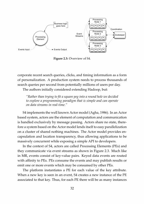
Figure 2.3: Overview of S4.

corporate recent search queries, clicks, and timing information as a formof personalization. A production system needs to process thousands ofsearch queries per second from potentially millions of users per day.

The authors initially considered extending Hadoop, but:

“Rather than trying to fit a square peg into a round hole we decidedto explore a programming paradigm that is simple and can operateon data streams in real-time.”

S4 implements the well known Actor model (Agha, 1986). In an Actorbased system, actors are the element of computation and communicationis handled exclusively by message passing. Actors share no state, there-fore a system based on the Actor model lends itself to easy parallelizationon a cluster of shared nothing machines. The Actor model provides en-capsulation and location transparency, thus allowing applications to bemassively concurrent while exposing a simple API to developers.

In the context of S4, actors are called Processing Elements (PEs) andthey communicate via event streams as shown in Figure 2.3. Much likein MR, events consist of key-value pairs. Keyed data events are routedwith affinity to PEs. PEs consume the events and may publish results oremit one or more events which may be consumed by other PEs.

The platform instantiates a PE for each value of the key attribute.When a new key is seen in an event, S4 creates a new instance of the PEassociated to that key. Thus, for each PE there will be as many instances

32

status.text:"Introducing #S4: a distributed #stream processing system"

PE1

PE2 PE3

PE4

RawStatusnulltext="Int..."

EVKEYVAL

Topictopic="S4"count=1

EVKEYVAL

Topictopic="stream"count=1

EVKEYVAL

TopicreportKey="1"topic="S4", count=4

EVKEYVAL

TopicExtractorPE (PE1)extracts hashtags from status.text

TopicCountAndReportPE (PE2-3)keeps counts for each topic acrossall tweets. Regularly emits report event if topic count is above a configured threshold.

TopicNTopicPE (PE4)keeps counts for top topics and outputs top-N topics to external persister

Figure 2.4: Twitter hashtag counting in S4.

as the number of different keys in the data stream. The instances arespread among the cluster to provide load balancing. Each PE consumesexactly those events whose key matches its own instantiation key.

A PE is implemented by defining a ProcessEvent function. This UDFis handed the current event, can perform any kind of computation andemit new keyed events on a stream. A communication layer will takecare of routing all the events to the appropriate PE. The user can definean application by specifying a DAG of PEs connected by event streams.

Unlike other systems S4 has no centralized master node. Instead,it leverages ZooKeeper to achieve a clean and symmetric cluster archi-tecture where each node provides the same functionalities. This choicegreatly simplifies deployments and cluster configuration changes.

Figure 2.4 presents a simple example of an S4 application that keepstrack of trending hashtag on Twitter. PE1 extracts the hashtags from thetweet and sends them down to PE2 and PE3 that increment their coun-ters. At regular intervals the counters are sent to an aggregator that pub-lishes the top-N most popular ones.

33

2.4 Algorithms

Data analysis researchers have seen in DISC systems the perfect tool toscale their computations to huge datasets. In the literature, there aremany examples of successful applications of DISC systems in differentareas of data analysis. In this section, we review some of the most signi-ficative example, with anl emphasis on Web mining and MapReduce.

Information retrieval has been the classical area of application forMR Indexing bags of documents is a representative application of thisfield, as the original purpose of MR was to build Google’s index for Websearch. Starting from the original algorithm, many improvements havebeen proposed, from single-pass indexing to tuning the scalability andefficiency of the process. (McCreadie et al., 2009a,b, 2011).

Several information retrieval systems have been built on top of MR.Terrier (Ounis et al., 2006), Ivory (Lin et al., 2009) and MIREX (Hiemstraand Hauff, 2010) enable testing new IR techniques in a distributed set-ting with massive datasets. These systems also provide state-of-the-artimplementation of common indexing and retrieval functionalities.

As we explain in Chapter 3, pairwise document similarity is a com-mon tool for a variety of problems such as clustering and cross-documentcoreference resolution. MR algorithms for closely related problems likefuzzy joins (Afrati et al., 2011a) and pairwise semantic similarity (Pan-tel et al., 2009) have been proposed. Traditional two-way and multiwayjoins have been explored by Afrati and Ullman (2010, 2011)

Logs are a gold mine of information about users’ preferences, natu-rally modeled as bags of lines. For instance frequent itemset mining ofquery logs is commonly used for query recommendation. Li et al. (2008)propose a massively parallel algorithm for this task. Zhou et al. (2009)design a DISC-based OLAP system for query logs that supports a vari-ety of data mining applications. Blanas et al. (2010) study several MR joinalgorithms for log processing, where the size of the bags is very skewed.

MapReduce has proven itself as an extremely flexible tool for a num-ber of tasks in text mining such as expectation maximization (EM) andlatent dirichlet allocation (LDA) (Lin and Dyer, 2010; Liu et al., 2011).

34

Mining massive graphs is another area of research where MapReducehas been extensively employed. Cohen (2009) presents basic patterns ofcomputation for graph algorithms in MR, while Lin and Schatz (2010)presents more advanced performance optimizations. Kang et al. (2011)propose an algorithm to estimate the graph diameter for graphs withbillions of nodes like the Web, which is by itself a challenging task.

Frequently computed metrics such as the clustering coefficient andthe transitivity ratio involve counting triangles in the graph. Tsourakakiset al. (2009) and Pagh and Tsourakakis (2011) propose two approachesfor approximated triangle counting on MR using randomization, whileYoon and Kim (2011) propose an improved sampling scheme. Suri andVassilvitskii (2011) propose exact algorithms for triangle counting thatscale to massive graphs on MapReduce.

MR has been used also to address NP-complete problems. Brocheleret al. (2010) and Afrati et al. (2011b) propose algorithms for subgraphmatching. Chierichetti et al. (2010) tackles the problem of max cover-ing, which can be applied to vertexes and edges in a graph. Lattanziet al. (2011) propose a filtering technique for graph matching tailored forMapReduce. In Chapter 4 we will present two MapReduce algorithmsfor graph b-matching with applications to social media.

A number of different graph mining tasks can be unified via general-ization of matrix operations. Starting from this observation, Kang et al.(2009) build a MR library for operation like PageRank, random walkswith restart and finding connected components. Co-clustering is the si-multaneous clustering of the rows and columns of a matrix in order tofind correlated sub-matrixes. Papadimitriou and Sun (2008) describe aMR implementation called Dis-Co. Liu et al. (2010) explore the problemof non-negative matrix factorization of Web data in MR.

Streaming on DISC system is still an unexplored area of research.Large scale general purpose stream processing platforms are a recent de-velopment. However, many streaming algorithms in the literature canbe adapted easily. For an overview of distributed stream mining algo-rithms see the book by Aggarwal (2007). For large scale stream miningalgorithms see Chapter 4 of the book by Rajaraman and Ullman (2010).

35

DISC technologies have also been applied to other fields, such as sci-entific simulations of earthquakes (Chen and Schlosser, 2008), collabo-rative Web filtering (Noll and Meinel, 2008) and bioinformatics (Schatz,2009). Machine learning has been a fertile ground for MR applicationssuch as prediction of user rating of movies (Chen and Schlosser, 2008).In general, many widely used machine learning algorithms can be im-plemented in MR (Chu et al., 2006).

36

Chapter 3

Similarity Self-Join inMapReduce

Similarity self-join computes all pairs of objects in a collection such thattheir similarity value satisfies a given criterion. For example it can beused to find similar users in a community or similar images in a set. Inthis thesis we focus on bags of Web pages. The inherent sparseness of thelexicon of pages on the Web allows for effective pruning strategies thatgreatly reduce the number of pairs to evaluate.

In this chapter we introduce SSJ-2 and SSJ-2R, two novel parallel al-gorithms for the MapReduce framework. Our work builds on state ofthe art pruning techniques employed in serial algorithms for similarityjoin. SSJ-2 and SSJ-2R leverage the presence of a distributed file systemto support communication patterns that do not fit naturally the MapRe-duce framework. SSJ-2R shows how to effectively utilize the sortingfacilities offered by MapReduce in order to build a streaming algorithm.Finally, we introduce a partitioning strategy that allows to avoid memorybottlenecks by arbitrarily reducing the memory footprint of SSJ-2R.

We present a theoretical and empirical analysis of the performanceof our two proposed algorithms across the three phases of MapReduce.Experimental evidence on real world data from the Web demonstratesthat SSJ-2R outperforms the state of the art by a factor of 4.5.

37

3.1 Introduction

In this chapter, we address the similarity self-join problem: given a col-lection of objects, we aim at discovering every pair of objects with highsimilarity, according to some similarity function. The task of discoveringsimilar objects within a given collection is common to many real worlddata mining and machine learning problems.

Item-based and user-based recommendation algorithms require to com-pute, respectively, pair-wise similarity among users or items. Due to thelarge number of users and objects commonly handled by popular recom-mender systems similarity scores are usually computed off-line.

Near duplicate detection is commonly performed as a pre-processingstep before building a document index. It may be used to detect redun-dant documents, which can therefore be removed, or it may be a hint todiscover content farms and spam websites exploiting content repurpos-ing strategies. Near duplicate detection finds application also in the areaof copyright protection as a tool for discovering plagiarism.

Density-based clustering algorithms like DBSCAN (Ester et al., 1996)or OPTICS (Ankerst et al., 1999) inherently join the input data based onsimilarity relationships. Correlation clustering (Bansal et al., 2004) usessimilarity relationship between the objects instead of the actual repre-sentation of the objects. All these algorithms will draw high benefit fromefficient and scalable MapReduce implementations of similarity joins.

Finding similar objects is also a basic step for data cleaning tasks. Whendealing with real world data, we wish to normalize different but simi-lar representations of the same entity, e.g. different names or addresses,caused by mistakes or formatting conventions. Similarity joins also playan important role in distance-based outlier detection.

We focus on document collections and model them as bags of vectors(see Section 1.2.1). Each document is a vector in a highly-dimensionalspace. Documents are a particular kind of data that exhibits a significantsparseness: only a small subset of the whole lexicon occurs in any givendocument. This sparsity allows to exploit pruning strategies that reducethe potentially quadratic number of candidate pairs to evaluate.

38

Finally, the size of the collection at hand poses new interesting chal-lenges. This is particularly relevant for Web-related collections, wherethe number of documents involved is measured in billions. For this set-ting, distributed solutions become mandatory. Indeed, there are a fewrelated proposals that exploit the MapReduce framework. Elsayed et al.(2008) propose a MapReduce algorithm to compute the similarity be-tween every pair of documents in a collection, without taking advantageof any pruning strategy. Vernica et al. (2010) present a MapReduce algo-rithm to compute the similarity join of collections of sets.

Our main contributions are the following.

• We present SSJ-2 and SSJ-2R the efficient distributed algorithmsbased on the MapReduce framework to compute the similarity self-join on a collection of documents.

• We borrow from existing pruning techniques designed for serialalgorithms, and we extend them to the distributed setting.

• We exploit selective communication patterns that do not naturallyfit the MapReduce paradigm.

• We provide detailed analytical and empirical analysis of the algo-rithms across the various phases of the MapReduce framework.

• We show that SSJ-2R performs nicely on a sample of the WT10gTREC Web Corpus.1

The rest of the chapter is organized as follows. In Section 3.2 we in-troduce the similarity self-join problem and some solutions adopted bynon-parallel algorithms. In Section 3.3 we discuss the algorithms for sim-ilarity self-join that are based on the MapReduce framework. Section 3.4presents our proposed algorithms, which are theoretically analyzed inSection 3.5 and experimentally evaluated in Section 3.6.

1http://ir.dcs.gla.ac.uk/test_collections/wt10g.html

39

3.2 Problem definition and preliminaries

We address the similarity self-join problem applied to a collection D ofdocuments. Let L be the lexicon of the collection. Each document d isrepresented as a |L|-dimensional vector. Without loss of generality, weassume that documents are normalized, so d[i] denotes the number ofoccurrences of the i-th term in the document d divided by the norm ‖d‖.We adopt the cosine distance to measure the similarity between two doc-uments. For normalized documents the cosine similarity can be simplycomputed as the inner product between document vectors.

Problem 1 (Similarity Self-Join Problem). Given a collection of normalizeddocument-vectorsD = {d1, . . . , dN}, a similarity function σ : D×D → R anda minimum similarity threshold σ, the Similarity Self-Join problem requires todiscover all those pairs di, dj ∈ D with similarity above the threshold:

σ(di, dj) =∑

0≤t<|L|

di[t] · dj [t] ≥ σ

Note that the results discussed in this chapter can be easily applied toother similarity measures, such as Jaccard, Dice or overlap.

Differently from normal join problems, self-join involves joining alarge table with itself. Thus it is not possible to apply traditional algo-rithms for data warehousing, that join a large fact table with smaller di-mension tables. Recent algorithms for log processing in MR also assumethat one of the tables is much smaller that the other (Blanas et al., 2010).

Following Arasu et al. (2006); Xiao et al. (2009), we classify algorithmsfor similarity self-join by their solution to the following sub-problems:

1. Signature scheme: a compact representation of each document;

2. Candidate generation: identifying potentially similar documentpairs given their signature;

3. Verification: computing document similarity;

4. Indexing: data structures for speeding up candidate generationand verification.

40

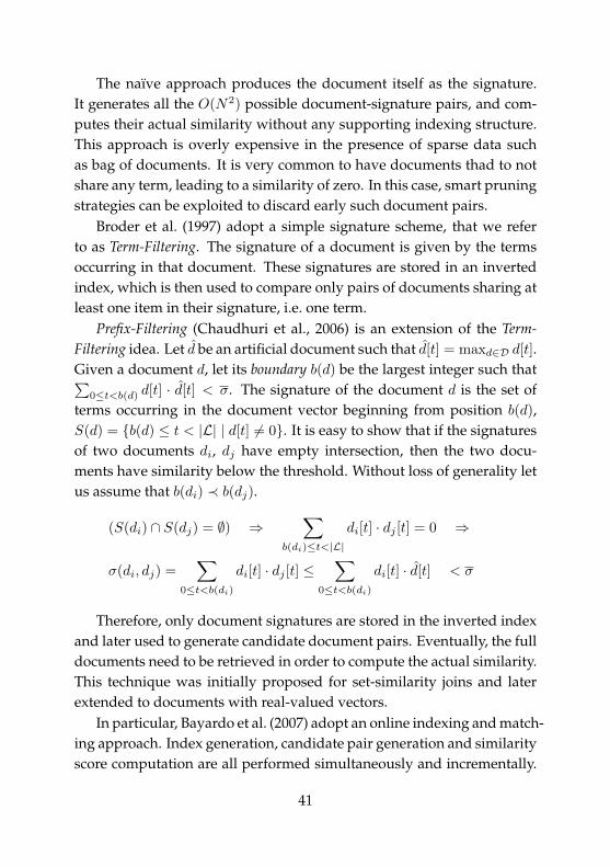
The naïve approach produces the document itself as the signature.It generates all the O(N2) possible document-signature pairs, and com-putes their actual similarity without any supporting indexing structure.This approach is overly expensive in the presence of sparse data suchas bag of documents. It is very common to have documents thad to notshare any term, leading to a similarity of zero. In this case, smart pruningstrategies can be exploited to discard early such document pairs.

Broder et al. (1997) adopt a simple signature scheme, that we referto as Term-Filtering. The signature of a document is given by the termsoccurring in that document. These signatures are stored in an invertedindex, which is then used to compare only pairs of documents sharing atleast one item in their signature, i.e. one term.

Prefix-Filtering (Chaudhuri et al., 2006) is an extension of the Term-Filtering idea. Let d be an artificial document such that d[t] = maxd∈D d[t].Given a document d, let its boundary b(d) be the largest integer such that∑

0≤t<b(d) d[t] · d[t] < σ. The signature of the document d is the set ofterms occurring in the document vector beginning from position b(d),S(d) = {b(d) ≤ t < |L| | d[t] 6= 0}. It is easy to show that if the signaturesof two documents di, dj have empty intersection, then the two docu-ments have similarity below the threshold. Without loss of generality letus assume that b(di) ≺ b(dj).

(S(di) ∩ S(dj) = ∅) ⇒∑

b(di)≤t<|L|

di[t] · dj [t] = 0 ⇒

σ(di, dj) =∑

0≤t<b(di)

di[t] · dj [t] ≤∑

0≤t<b(di)

di[t] · d[t] < σ

Therefore, only document signatures are stored in the inverted indexand later used to generate candidate document pairs. Eventually, the fulldocuments need to be retrieved in order to compute the actual similarity.This technique was initially proposed for set-similarity joins and laterextended to documents with real-valued vectors.

In particular, Bayardo et al. (2007) adopt an online indexing and match-ing approach. Index generation, candidate pair generation and similarityscore computation are all performed simultaneously and incrementally.

41

Each document is matched against the current index to find potentialcandidates. The similarity scores are computed by retrieving the candi-date documents directly from the collection. Finally, a signature is ex-tracted from the current document and added to the index.

This approach results in a single full scan of the input data, a smallnumber of random accesses to single documents, and a smaller (on av-erage) index to be queried. Prefix-filtering outperforms alternative tech-niques such as LSH (Gionis et al., 1999), PartEnum (Arasu et al., 2006)and ProbeCount-Sort (Sarawagi and Kirpal, 2004), which we thereforedo not considered in our work. Unfortunately, an incremental approachthat leverages a global shared index is not practical on a large parallelsystem because of contention on the shared resource.

Finally, Xiao et al. (2008) present some additional pruning techniquesbased on positional and suffix information. However these techniquesare specifically tailored for set-similarity joins and cannot be directly ap-plied to document similarity.

3.3 Related work

In this section we describe two MR algorithm for the similarity self-joinproblem. Each exploits one of the pruning techniques discussed above.

3.3.1 MapReduce Term-Filtering (ELSA)

Elsayed et al. (2008) present a MapReduce implementation of the Term-Filtering method. Hereafter we refer to it as ELSA for convenience. Theauthors propose an algorithm for computing the similarity of every doc-ument pair, which can be easily adapted to our setting by adding a sim-ple post-filtering. The algorithm runs two consecutive MR jobs, the firstbuilds an inverted index and the second computes the similarities.

Indexing: Given a document di, for each term, the mapper emits the termas the key, and a tuple 〈i, di[t]〉 consisting of document ID and weight asthe value. The shuffle phase of MR groups these tuples by term anddelivers these inverted lists to the reducers, that write them to disk.

42

Map : 〈i, di〉 → [〈t, 〈i, di[t]〉〉 | di[t] > 0]

Reduce : 〈t, [〈i, di[t]〉, 〈j, dj [t]〉, . . .]〉 → [〈t, [〈i, di[t]〉, 〈j, dj [t]〉, . . .]〉]

Similarity: Given the inverted list of term t, the mapper produces thecontribution wij [t] = di[t] · dj [t] for every pair of documents where theterm t co-occurs. This value is associated with a key consisting of the pairof document IDs 〈i, j〉. For any document pair the shuffle phase will passto the reducer the contribution list Wij = {wij [t] | wij [t] > 0, ∀t ∈ L}from the various terms, which simply need to be summed up.

Map : 〈t, [〈i, di[t]〉, 〈j, dj [t]〉, . . .]〉 → [〈〈i, j〉, wij [t]〉]

Reduce : 〈〈i, j〉,Wij〉 →

〈〈i, j〉, σ(di, dj) =∑

w∈Wij

w〉

The Term-Filtering is exploited implicitly: the similarity of two doc-

uments that do not share any term is never evaluated because none oftheir terms ever occurs in the same inverted list.

The main drawback of this approach is caused by the large numberof candidate document pairs that it generates. In fact, there are manydocument pairs that share only a few terms but have anyway a simi-larity largely below the threshold. The number of candidates directlyaffects completion time. More importantly it determines the shuffle size,the volume of intermediate data to be moved from mappers to reducers.Minimizing shuffle size is critical because network bandwidth is the onlyresource that cannot be easily added to a cluster.

Finally, recall that reducers may start only after every mapper hascompleted. Therefore, the presence of a few long inverted lists for com-mon terms induces a significant load imbalance. Most of the resourceswill remain idle until the processing of the longest inverted list is com-pleted. To alleviate this issue Elsayed et al. remove the top 1% most fre-quent terms, thus trading efficiency for precision. Our goal is to providean efficient algorithm that computes the exact similarity.

43

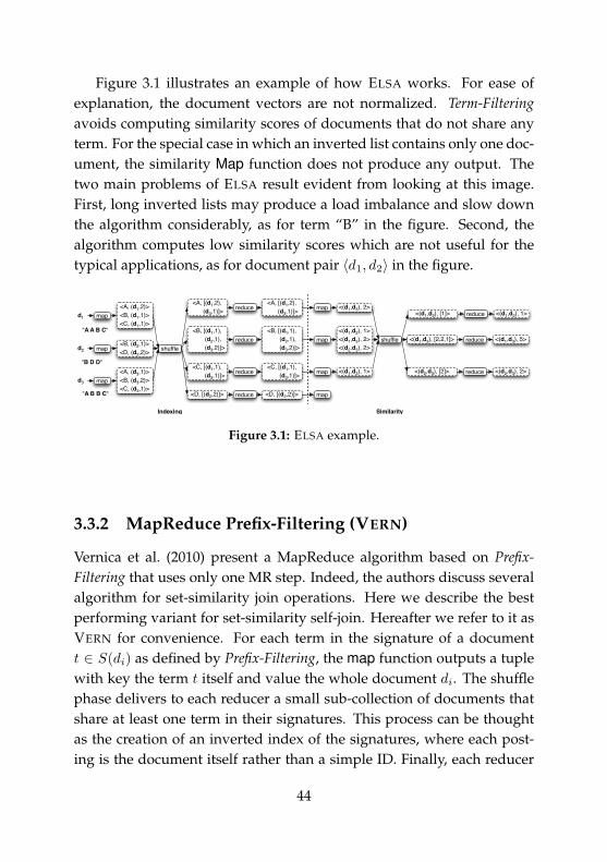
Figure 3.1 illustrates an example of how ELSA works. For ease ofexplanation, the document vectors are not normalized. Term-Filteringavoids computing similarity scores of documents that do not share anyterm. For the special case in which an inverted list contains only one doc-ument, the similarity Map function does not produce any output. Thetwo main problems of ELSA result evident from looking at this image.First, long inverted lists may produce a load imbalance and slow downthe algorithm considerably, as for term “B” in the figure. Second, thealgorithm computes low similarity scores which are not useful for thetypical applications, as for document pair 〈d1, d2〉 in the figure.

shuffle

map

map

map

map

shuffle<B, [(d1,1),

(d2,1), (d3,2)]>

<C, [(d1,1), (d3,1)]>

<D, [(d2,2)]>

<A, [(d1,2),(d3,1)]>

<A, (d1,2)><B, (d1,1)><C, (d1,1)>

<B, (d2,1)><D, (d2,2)>

<A, (d3,1)><B, (d3,2)><C, (d3,1)>

<B, [(d1,1),(d2,1),

(d3,2)]>

<A, [(d1,2),(d3,1)]>

<C, [(d1,1), (d3,1)]>

<D, [(d2,2)]>

reduce

reduce

reduce

reduce

Indexing Similarity

<(d1,d2), 1><(d1,d3), 2><(d2,d3), 2>

<(d1,d3), 1>

<(d1,d3), 2>

<(d1,d3), [2,2,1]>

<(d1,d2), [1]>

<(d2,d3), [2]>

reduce

reduce

reduce

<(d1,d3), 5>

<(d1,d2), 1>

<(d2,d3), 2>

mapd1

"A A B C"

mapd3

"A B B C"

mapd2

"B D D"

Figure 3.1: ELSA example.

3.3.2 MapReduce Prefix-Filtering (VERN)

Vernica et al. (2010) present a MapReduce algorithm based on Prefix-Filtering that uses only one MR step. Indeed, the authors discuss severalalgorithm for set-similarity join operations. Here we describe the bestperforming variant for set-similarity self-join. Hereafter we refer to it asVERN for convenience. For each term in the signature of a documentt ∈ S(di) as defined by Prefix-Filtering, the map function outputs a tuplewith key the term t itself and value the whole document di. The shufflephase delivers to each reducer a small sub-collection of documents thatshare at least one term in their signatures. This process can be thoughtas the creation of an inverted index of the signatures, where each post-ing is the document itself rather than a simple ID. Finally, each reducer

44

finds similar pairs among candidates by using state-of-the-art serial algo-rithms (Xiao et al., 2008). The Map and Reduce functions are as follows.

Map : 〈i, di〉 → [〈t, di〉 | t ∈ S(di)]

Reduce : 〈t,Dv = [di, dj , . . .]〉 → [〈〈i, j〉, σ(di, dj)〉 | di, dj ∈ Dv]

Nonetheless, this approach does not bring a significant improvementover the previous strategy. First, a document with a signature of lengthn is replicated n times, even if there are no other documents with anoverlapping signature. Second, pairs of similar documents that have mcommon terms in their signatures are produced m times at different re-ducers. Computing these duplicates is a overhead of parallelization, andtheir presence requires a second scan of the output to get rid of them.

Figure 3.2 illustrates an example run of VERN. Light gray terms arepruned from the document by using Prefix-Filtering. Each document isreplicated once for each non-pruned term it contains. Finally, the reducercomputes the similarity of the bag of documents it receives by employ-ing a serial SSJ algorithm. As shown in Figure 3.2, VERN computes thesimilarity of the pair 〈d1, d3〉multiple times at different reducers.

We propose here a simple strategy that solves the issue of duplicatesimilarity computation. We use this modified version of the originalVERN algorithm in our evaluation. This modified version runs slightlybut consistently faster than the original one, and it does not require post-processing. The duplicate similarities come from pair of documents thatshare more than one term in their signatures. Let Sij = S(di) ∩ S(dj)

be the set of such shared terms in document pair 〈di, dj〉. Let t be thelast of such terms in the order imposed to the lexicon by Prefix-Filteringt = tx | tx � ty ∀ tx, ty ∈ Sij . The reducer that receives each pair cansimply check if its key corresponds to t and compute the similarity onlyin this case. The term t for each pair of documents can be efficiently com-puted by a simple backwards scan of the two arrays that represent thedocuments. This strategy allows to avoid computing duplicate similari-ties and does not impose any additional overhead the original algorithm.

45

shuffle

<(d1,d3), 5>

<(d1,d3), 5>

<A, (d1, A A B C)><B, (d1, A A B C)><C, (d1, A A B C)>

<D, (d2, B D D)>

<B, (d3, A B B C)><C, (d3, A B B C)>

mapd1

"A A B C"

mapd2

"B D D"

mapd3

"A B B C"

<B, [(d1, A A B C),(d3, A B B C)]>

<A, (d1, A A B C)>

<C, [(d1, A A B C),(d3, A B B C)]>

<D, [(d2, B D D)]>

reduce

reduce

reduce

reduce

Figure 3.2: VERN example.

3.4 SSJ Algorithms

In this section we describe two algorithms based on Prefix-Filtering thatovercome the weak points of the algorithms presented above. The firstalgorithm, named SSJ-2, performs a Prefix-Filtering in two MR steps.Note that in the first step we use a naïve indexing algorithm but if neededmore advanced techniques can be used (McCreadie et al., 2009b, 2011).The second algorithm, named SSJ-2R, additionally uses a remainder fileto broadcast data that is likely to be used by every reducer. It also effec-tively partitions the search space to reduce the memory footprint. Codefor both algorithm is open source and available online.2

3.4.1 Double-Pass MapReduce Prefix-Filtering (SSJ-2)

This algorithm is and extention of ELSA, and also consists of an indexingphase followed by a similarity computation phase.

SSJ-2 shortens the inverted lists by employing Prefix-Filtering. Asshown in Figure 3.3, the effect of Prefix-Filtering is to reduce the portionof document indexed. The terms occurring in di up to position b(di), orbi for short, need not be indexed. By sorting terms in decreasing order offrequency, the most frequent terms are discarded. This pruning shortensthe longest inverted lists and brings a significant performance gain.

2https://github.com/azaroth/Similarity-Self-Join

46

To improve load balancing we employ a simple bucketing techniqueDuring the indexing phase we randomly hash the inverted lists to differ-ent buckets. This spreads the longest lists uniformly among the buckets.Each bucket is then consumed by a different mapper in the next phase.

Pruned Indexed

Pruned Indexed

di

dj

bi bj

|L|0

Figure 3.3: Pruned document pair: the left part (orange/light) has beenpruned, the right part (blue/dark) has been indexed.

Unfortunately with this schema the reducers do not have enough in-formation to compute the similarity between di and dj . They receive onlythe contribution from terms t � bj , assuming bi ≺ bj . For this reason, thereducers need two additional remote I/O operations to retrieve the twodocuments di and dj from the underlying distributed file system.

SSJ-2 improves over both ELSA and VERN in terms of the amountof intermediate data produced. Thanks to Prefix-Filtering, the invertedlists are shorter than in ELSA and therefore the number of candidatepairs generated decreases quadratically. In VERN each document is al-ways sent to a number of reducers equal to the size of its signature, evenif no other document signature shares any term with it. In SSJ-2 a pair

47

of documents is sent to the reducer only if they share at least one termin their signature. Furthermore, while SSJ-2 computes the similarity be-tween any two given documents just once, VERN computes the similarityof two documents in as many reducers as the size of the intersection oftheir signatures. Therefore, SSJ-2 has no computational overhead due toparallelization, and significantly reduces communication costs.

Figure 3.4 presents an example for SSJ-2. As before, light gray termshave been pruned and documents are not normalized to ease the expla-nation. Pairs of documents that are below the similarity threshold arediscarded early. However the reducer of the similarity phase needs toaccess the remote file system to retrieve the documents in order to com-pute the correct final similarity score.

shuffle

<(d1,d3), 2>

<(d1,d3), 1>

<(d1,d3), [2,1]> reduce <(d1,d3), 5>

HDFS

d3"A B B C"

d1"A A B C"

Similarity

map

map

map

shuffle

<B, [(d1,1), (d3,2)]>

<C, [(d1,1), (d3,1)]>

<D, [(d2,2)]>

<B, (d1,1)><C, (d1,1)>

<D, (d2,2)>

<B, (d3,2)><C, (d3,1)>

mapd1

"A A B C"

mapd2

"B D D"

mapd3

"A B B C"

<B, [(d1,1), (d3,2)]>

<C, [(d1,1), (d3,1)]>

<D, [(d2,2)]>

reduce

reduce

reduce

Indexing

Figure 3.4: SSJ-2 example.

48

3.4.2 Double-Pass MapReduce Prefix-Filtering with Re-mainder File (SSJ-2R)

For any given pair of documents 〈di, dj〉, the reducers of SSJ-2 receiveonly partial information. Therefore, they need to retrieve the full docu-ments in order to correctly compute their similarity. Since a node runsmultiple reducers over time, each of them remotely accessing two doc-uments, in the worst case this is equivalent to broadcasting the full col-lection to every node, with obvious limitations to the scalability of thealgorithm. We thus propose an improved algorithm named SSJ-2R thatdoes not perform any remote random access, and that leverages the non-indexed portion of the documents.

Let us make a few interesting observations. First, some of the termsare very common, and therefore used to compute the similarity of mostdocument pairs. For those terms, it would be more efficient to broad-cast their contributions rather than pushing them through the MR frame-work. Indeed, such piece of information is the one pruned via Prefix-Filtering during the indexing phase. We thus propose to store the prunedportion of each document in a remainder file DR, which can be later re-trieved by each reducer from the underlying distributed file system.

Second, the remainder file DR does not contain all the informationneeded to compute the final similarity. Consider Figure 3.3, each reducerreceives the contributions wij [t] = di[t] · dj [t] | t � bj . DR contains in-formation about the terms di[t] | t ≺ bi} and {dj [t] | t ≺ bj . But, subtly,no information is available for those terms di[t] | bi � t ≺ bj . On theone hand, those term weights are not in the remainder file because theyhave been indexed. On the other hand, the corresponding inverted listscontain the frequency of the terms in di but not of those occurring in dj ,and therefore, the weights wij [t] = di[t] · dj [t] cannot be produced.

We thus propose to let one of the two documents be delivered tothe reducer through the MR framework by shuffling it together with theweights of the document pairs. Given two documents di and dj as shownin Figure 3.3, if bi ≺ bj we call di the Least Pruned Document and dj theMost Pruned Document. Our goal is to group at the reducer each docu-

49

ment dwith the contributionsw of every document pair 〈di, dj〉 for whichd is the least pruned document between di and dj . This document con-tains the pieces of information that we are missing in order to computethe final similarity score. This can be achieved by properly defining thekeys produced by the mappers and their sorting and grouping operators.

More formally, we define two functions LPD(di, dj) and MPD(di, dj).

LPD(di, dj) =

{i, if bi ≺ bjj, otherwise

MPD(di, dj) =

{j, if bi ≺ bji, otherwise

First, we slightly modify the similarity Map function such that for ev-ery document pair of the given inverted list, it produces as keys a coupleof document IDs where the first is always the LPD, and as values theMPD and the usual weight w.

Map : [〈t, [〈i, di[t]〉, 〈j, dj [t]〉, . . .]〉]→[〈〈LPD(di, dj),MPD(di, dj)〉 , 〈MPD(di, dj), wij [t]〉〉]

Second, we take advantage of the possibility of running independentMap functions whose outputs are then shuffled together. We define aMap function that takes the input collection and outputs its documents.

Map : 〈i, di〉 → [〈〈i, φ〉 , di〉]

where φ is a special value such that φ < i ∀di ∈ D.Third, we make use of the possibility offered by Hadoop to rede-

fine parts of its communication pattern. The process we describe hereis commonly known as secondary sort in MR parlance. We redefine thekey partitioning function, which selects which reducer will process thekey. Our function takes into account only the first document ID in thekey. This partitioning scheme guarantees that all the key-value pairs thatshare the same LPD will end up in the same partition, together with onecopy of the LPD document itself coming from the second Map function.

We instruct the shuffle phase of MR to sort the keys in each partitionin ascending order. This order takes into account both IDs, the first asprimary key and the second as secondary key. Consequently, for each

50

document di MR builds a list of key-value pairs such that the first key is〈i, φ〉, followed by every pair of document IDs for which di is the LPD.

Finally, we override the grouping function, which determines whethertwo keys belong to the same equivalence class. If two keys are equiva-lent, their associated values will be processed by the same single call tothe Reduce function. Concretely, the grouping function builds the argu-ment list for a call to the Reduce function by selecting values from thepartition such that the corresponding keys are equivalent. Therefore ourgrouping function must consistent with our partitioning scheme: twokeys 〈i, j〉 and 〈i′, j′〉 are equivalent iff i = i′.

The input of the Reduce function is thus as follows.

〈〈i, φ〉 , [di, 〈j, wij [t′]〉 , 〈j, wij [t′′]〉 , . . . , 〈k,wik[t′]〉 , 〈k,wik[t′′]〉 , . . .]〉

The key is just the first key in the group, as they are all equivalent toMR. The first value is the LPD document di. Thanks to the sorting of thekeys, it is followed by a set of contiguous stripes of weights. Each stripeis associated to the same document dj | j = MPD(di, dj).

SSJ-2R can now compute the similarity σ(di, dj) in one pass. Beforethe algorithm starts, each reducer loads the remainder file DR in mem-ory. For each Reduce call, SSJ-2R starts by caching di, which is at thebeginning of the list of values. Then, for each dj in the list, it sums up allthe corresponding weights wij to compute a partial similarity. Finally, itretrieves the pruned portion of dj from DR, computes the similarity ofdi to the pruned portion of dj and adds this to the partial similarity com-puted before. This two step process correctly computes the final similar-ity σ(di, dj) because all the terms bi � t ≺ bj are available both in di andin the pruned portion of dj . This process is repeated for each stripe ofweights belonging to the same document pair in the list of values.

Differently from SSJ-2, SSJ-2R performs no remote access to the doc-ument collection. Given a document pair, one is delivered fully throughthe MapReduce framework, and the other is partially retrieved from theremainder file DR. The advantage in terms of communication costs isgiven by the remainder file. Indeed, DR is much smaller than the inputcollection. We show experimentally that its size is one order of magni-

51

tude smaller than the input. Therefore,DR can be efficiently broadcast toevery node through the distributed file system. Each reducer can load itin main memory so that the similarity computation can be fully accom-plished without any additional disk access.

Figure 3.5 illustrates the full data flow of SSJ-2R with an example. Asbefore, light gray terms have been pruned and documents are not nor-malized. SSJ-2R stores the pruned part of each document in the remain-der file, which is put in the distributed cache in order to be broadcast.The reducer of the similarity phase reads the remainder file in memorybefore starting to process its value list. In the example, d1 is deliveredthrough the MR framework, while the pruned part of d3 is recoveredfrom the remainder file. This procedure allows to correctly compute thecontributions of the term “A” which was pruned from the documents.The contributions from terms “B” and “C” are computed by the mapperof the similarity phase and delivered normally through MR.

3.4.3 Partitioning

Even though the remainder fileDR is much smaller than the original col-lection, its size will grow when increasing the collection size, and there-fore it may hinder the scalability of the algorithm.

To overcome this issue, we introduce a partitioning scheme for theremainder file. Given a user defined parameter K, we split the range ofdocument identifiers into K equally sized chunks, so that the unindexedportion of document di falls into the bi/Kc-th chunk. Consequently, wemodify the partitioning function which maps a key emitted by the map-per to a reducer. We map each key 〈i, j〉 to the bj/Kc-th reducer instance,i.e. the mapping is done on the basis of the MPD. This means that eachreducer will receive only weights associated to a portion of the documentspace. Therefore, the reducer needs to retrieve and load in memory only1/K-th of the remainder file DR.

This new partitioning scheme spreads the weights associated to thesame LPD document over K different reducers. Therefore, to correctlycompute the final similarity SSJ-2R needs a copy of the LPD document

52

shuffle

<B, [(d1,1), (d3,2)]>

<C, [(d1,1), (d3,1)]>

<D, [(d2,2)]>

<B, (d1,1)><C, (d1,1)>

<D, (d2,2)>

<B, (d3,2)><C, (d3,1)>

mapd1

"A A B C"

mapd2

"B D D"

mapd3

"A B B C"

<B, [(d1,1), (d3,2)]>

<C, [(d1,1), (d3,1)]>

<D, [(d2,2)]>

reduce

reduce

reduce

Indexing

shuffle

<(d1,d3), 2>

<(d1,d3), 1>

<(d1,✦),"A A B C"><(d1,d3), 2><(d1,d3), 1>

reduce <(d1,d3), 5>

Similarity

map

map

map

map

Remainder File

d1 "A A"

d3 "A"

d2 "B"Distributed Cache

<(d1,✦),"A A B C">

<(d3,✦),"A B B C">

Figure 3.5: SSJ-2R example.

di at each of these reducers. For this reason, we replicate K times thespecial key 〈i, φ〉 and its associated value di, once for each partition.

The parameter K allows to tune the memory usage of SSJ-2R andcontrols the tradeoff with the communication cost due to replication.

3.5 Complexity analysis

In Section 2.2.1 we presented a few proposals for modeling MapReducealgorithms (Afrati and Ullman, 2009; Karloff et al., 2010). Indeed, esti-mating the cost of a MapReduce algorithm is quite difficult, because of

53

Table 3.1: Symbols and quantities.

Symbol Description

d d Avg. and Max. document lengths s Avg. and Max. signature lengthp p Avg. and Max. inverted list length with Prefix-Filteringl Avg. inverted list length without pruningr Cost of a remote access to a documentR Cost of retrieving the remainder file DR

Table 3.2: Complexity analysis.

ALGORITHM Map Shuffle ReduceELSA l2 |L| · l2 d

VERN s · d |D| · s · d p2 · dSSJ-2 p2 |L| · p2 d+ r

SSJ-2R p2 |L| · p2 + |D| · d+R d

the inherent parallelism, the hidden cost of the shuffling phase, the over-lap among computation and communication managed implicitly by theframework, the non-determinism introduced by combiners and so on.

We prefer to model separately the three main steps of a MapReducejobs: the Map and Reduce functions, and the volume of the data to beshuffled. In particular, we take into consideration the cost associatedto the function instance with the largest input. This way, we roughlyestimate the maximum possible degree of parallelism and we are able tocompare the different algorithms in deeper detail.

We refer to Table 3.1 for the symbols used in this section. The quantityl can also be seen as the average frequency of the terms in the lexicon L.Similarly, p can also be seen as the number of signatures containing anygiven term. Clearly, it holds that p ≤ l.

The running time of ELSA is dominated by the similarity phase. Its

54

Map function generates every possible document pair for each invertedlist, with a cost of O(l2). Most of this large number of candidate pairshas a similarity below the threshold. Furthermore, the presence of longinverted lists introduces stragglers. Since reducers may start only afterevery mapper has completed, mappers processing the longest lists keepresources waiting idly. Since the shuffling step handles a single datumfor every generated pair, we can estimate the cost by summing over thevarious inverted lists asO(|L| · l2). The Reduce function just sums up thecontributions of the various terms, with a cost O(d).

VERN runs only one MR job. The Map replicates each document d|S(d)| times, with a cost of O(s · d). Similarly, we can estimate the shufflesize as O(|D| · d · s). The Reduce evaluates the similarity of every pairof documents in its input, with cost O(p2 · d). Due to Prefix-Filtering, themaximum reducer input size is p, which is smaller than l.

By comparing the two algorithms, we notice the superiority of VERN

in the first two phases of the computation. The Map function generates anumber of replicas of each document, rather then producing a quadraticnumber of partial contributions. Considering that |L| · l is equal to |D| ·d,and that l is likely to be much larger than s, it is clear that ELSA has thelargest shuffle size. Conversely, the Reduce cost for VERN is quadraticin the size of the pruned lists p.

Our proposed algorithms SSJ-2 and SSJ-2R have a structure simi-lar to ELSA. The Map cost O(p2) depends on the pruned inverted lists.For SSJ-2R, we are disregarding the cost of creating replicas of the inputin the similarity Map function, since it is much cheaper than processingthe longest inverted list. They have similar shuffles sizes, respectivelyO(|L| · p2) and O(|L| · p2 + |D| · d + R). In this case we need to con-sidered the cost of shuffling the input documents and the remainder filegenerated by SSJ-2R. Note that we are considering the remainder file asa shuffle cost even though it is not handled by MapReduce. Finally, theReduce cost is different. In addition to the contributions coming fromthe pruned inverted index, SSJ-2 needs to access documents remotelywith a total cost of O(d + r). Conversely SSJ-2R has a cost of O(d) sincethe unindexed portion of the document is already loaded in memory at

55

the local node, delivered via the distributed file system.Thanks to Prefix-Filtering, the Map cost of our proposed algorithm

smaller than ELSA, yet larger than VERN. For the same reason, the shuf-fle size of SSJ-2 is smaller than ELSA but still larger than VERN, if weassume that p is not significantly smaller than l. For SSJ-2R, the shufflesize is probably its weakest point. Shuffling the whole collection withinthe MapReduce data flow increases the volume of intermediate data. TheReduce function of SSJ-2 needs to remotely recover the documents be-ing processed to retrieve their unindexed portions. This dramaticallyincreases its cost beyond ELSA but can hardly be compared with VERN.SSJ-2R has about the same cost as ELSA when assuming that the remain-der file is already loaded in memory.

It is difficult to combine the costs of the various phases of the fouralgorithms. Therefore, it is not possible to understand which is the best.We can conclude that Elsayed et al. is the worst of the four, due to the nonexploitation of the Prefix-Filtering, and that the impact of the shufflingphase will determine the goodness of our proposed algorithms. In theexperimental section, we evaluate empirically the efficiency of the fouralgorithms in the three steps of the MapReduce framework.

3.6 Experimental evaluation

In this section we describe the performance evaluation of the algorithms.We used several subsets of the TREC WT10G Web corpus. The originaldataset has 1,692,096 english language documents. The size of the entireuncompressed collection is around 10GiB. In Table 3.3 we describe thesamples of the collection we used, ranging from ∼ 17k to ∼ 63k docu-ments. We preprocessed the data to prepare it for analysis. We parsedthe dataset stripping HTML, removed stop-words, performed stemmingand vectorization of the input and extracted the lexicon. We also sortedthe features inside each document in decreasing order of term frequencyin order to effectively utilize Prefix-Filtering.

We ran the experiments on a 5-node cluster. Each node was equippedwith two Intel Xeon E5520 CPUs @2.27GHz, with 8 virtual cores (for a

56

Table 3.3: Samples from the TREC WT10G collection.

D17K D30K D63K# documents 17,024 30,683 63,126# terms 183,467 297,227 580,915# all pairs 289,816,576 941,446,489 3,984,891,876# similar pairs 94,220 138,816 189,969

total of 80 virtual cores), a 2TiB disk, 8GiB of RAM, and Gigabit Ethernet.We used one of the nodes to run Hadoop’s master daemons (NameN-

ode and JobTracker), the rest were configured as slaves running DataN-ode and TaskTracker daemons. Two of the virtual cores on each slavemachine were reserved to run the daemons, the rest were equally splitamong map and reduce slots (7 each), for a total of 28 slots for each phase.

We tuned Hadoop’s configuration as follows: we allocated 1GiB ofmemory to each daemon and 400MiB to each task, changed the blocksize of HDFS to 256MiB and the file buffer size to 128KiB, disabled spec-ulative execution and enabled JVM reuse and map output compression.

For each algorithm, we wrote an appropriate combiner to reduce theshuffle size (a combiner is a reduce-like function that runs inside themapper to aggregate partial results). For SSJ-2 and SSJ-2R the combinerperform the sums of partial scores in the values, according to the samelogic used in the reducer. We also implemented raw comparators for ev-ery key type used in order to get better performance (raw comparatorscompare keys during sorting without deserializing them into objects).

3.6.1 Running time

We compared the four algorithms described in the previous sections. Thetwo baselines ELSA and VERN and the two algorithms proposed by us:SSJ-2 and SSJ-2R. VERN would require an additional step for removingduplicate similar pairs. We did not need to implement this step thanksto the strategy described in Section 3.3.2 Therefore our analysis does nottake into account the overhead induced by such duplicate removal.

For SSJ-2R we used a partitioning factor of the remainder file K = 4.

57

0

10000

20000

30000

40000

50000

60000

15000 20000 25000 30000 35000 40000 45000 50000 55000 60000 65000

Tim

e (

se

co

nd

s)

Number of vectors

ELSAVERNSSJ-2

SSJ-2R

Figure 3.6: Running time.

We enabled partitioning just for the sake of completeness, given that themappers were not even close to fill the available memory.

We use 56 mappers and 28 reducers, so that the mappers finish intwo waves and all the reducers can start copying and sorting the partialresults while the second wave of mappers is running. For all the experi-ments, we set the similarity threshold σ = 0.9.

Figure 3.6 shows the running times of the four different algorithms.All of them have a quadratic step, so doubling the size of the inputroughly multiplies by 4 the running time. Unexpectedly, VERN does notimprove significantly over ELSA. This means that Prefix-Filtering is notfully exploited. Recall ELSA uses a simple Term-Filtering and comparesany document pair sharing at least one term. Both our proposed algo-rithms outperform the two baselines. In particular, SSJ-2 is more thantwice faster than VERN and SSJ-2R is about 4.5 times faster. Notice that

58

SSJ-2R is twice as fast compared to SSJ-2, which means that the im-provement given by the use of the remainder file is significant.

We tried to fit a simple power law model f(x) = axb to the runningtime of the algorithms. For all algorithms but VERN the parameter b u2.5, while a u 10−8 with ELSA having the largest one. VERN has a smallerconstant a u 10−10 with a larger b u 2.9. However, given the smallnumber of data points available the analysis is not conclusive.

3.6.2 Map phase

0

1000

2000

3000

4000

5000

6000

7000

8000

15000 20000 25000 30000 35000 40000 45000 50000 55000 60000 65000

Tim

e (

se

co

nd

s)

Number of vectors

ELSAVERNSSJ-2

SSJ-2R

Figure 3.7: Average mapper completion time.

In Figure 3.7 we report the average map times for each algorithm.Clearly VERN is the fastest. The mapper only replicates input docu-ments. The time required by the other algorithms grows quadraticallyas expected. The two algorithms we propose are two times faster thanELSA for two main reasons.

59

0

200

400

600

800

1000

1200

1400

1600

1800

2000

0 10 20 30 40 50

Tim

e (

se

co

nd

s)

Mapper ID

ELSAVERN

SSJ-2R without bucketingSSJ-2R with bucketing

Figure 3.8: Mapper completion time distribution.

First, Prefix-Filtering reduces the maximum inverted list length. Evena small improvement here brings a quadratic gain. Since Prefix-Filteringremoves the most frequent terms, the longest inverted lists are short-ened or even removed. For D17K, the length of the longest inverted listis reduced from 6600 to 1729 thanks to Prefix-Filtering, as shown in Fig-ure 3.9. The time to process such inverted list decreases dramatically, andalso the amount of intermediate data generated is reduced. Interestingly,Prefix-Filtering does not affect significantly the index size. Only 10% ofthe index is pruned as reported in Table 3.4, meaning that its effects arelimited to shortening the longest inverted lists.

Second, we employ a bucketing technique to improve load balancing.Since mappers process the inverted lists in chunks, the longest invertedlists might end up in the same chunk and be processed by a single map-per. SSJ-2 and SSJ-2R randomly hash the inverted lists into different

60

Table 3.4: Statistics for the four algorithms on the three datasets.D

atas

et

Alg

orit

hm

#ev

alua

ted

pair

s(M

)

Inde

xsi

ze(M

B)

Rem

aind

ersi

ze(M

B)

Shuf

flesi

ze(G

B)

Run

ning

tim

e(s

)

Avg

.map

tim

e(s

)

Std.

map

tim

e(%

)

Avg

.red

uce

tim

e(s

)

Std.

redu

ceti

me

(%)

D17

K

ELSA 109 46 3.3 2,187 276 127.50 49 16.68VERN 401 3.7 1,543 42 68.10 892 22.20SSJ-2 65 41 2.1 971 148 37.92 575 3.58

SSJ-2R 65 41 4.7 2.6 364 122 26.50 49 15.50

D30

K

ELSA 346 92 11.3 8,430 1,230 132.08 82 15.91VERN 1,586 8.3 5,313 112 68.10 3,847 13.94SSJ-2 224 82 8.1 3,862 635 32.06 2,183 5.81

SSJ-2R 224 82 8.2 10.5 1,571 560 23.41 155 15.50

D63

K

ELSA 1,519 189 49.2 51,540 7,013 136.39 1,136 11.84VERN 6,871 20.7 28,534 338 59.61 16,849 9.36SSJ-2 1,035 170 35.8 20,944 3,908 24.32 11,328 2.76

SSJ-2R 1,035 170 15.6 49.7 9,745 3,704 20.26 846 12.11

buckets, so that the longest lists are likely spread among all the map-pers. Figure 3.8 shows the completion time of the mappers for the D17Kdataset. VERN has the lowest average mapper completion time, as allthe work is done in the reducer. However, due to skew in the input, theslowest mapper in VERN is slower than in SSJ-2R with bucketing. Thiscan happen if there are a few very dense documents in the input, so thatVERN needs to create a large number of copies of each of these docu-ment. ELSA is in any case slower than SSJ-2R without bucketing justbecause of the maximum inverted list length. Nevertheless, completiontimes are not evenly distributed in ELSA. This skew induces a strongload imbalance, forcing all the reducers to wait the slowest mapper be-fore starting. Bucketing solves this issue by evenly spreading the loadamong mappers. As a result, the running time of the slowest mapper isalmost halved. The standard deviation of map completion times for allalgorithms is reported in Table 3.4.

61

1

10

100

1000

100 1000

Nu

mb

er

of

lists

Inverted list length

max=6600

ELSA

1

10

100

1000

Nu

mb

er

of

lists

max=1729

SSJ-2R

Figure 3.9: Effect of Prefix-filtering on inverted list length distribution.

3.6.3 Shuffle size

Figure 3.10 shows the shuffles sizes for the various algorithms whenvarying the input size. The shuffle size is affected by the combiners, thatcompact the key-value pairs emitted by the mappers into partial resultsby applying a reduce-like function. VERN has the smallest shuffle size.We intuitively expected that the replication performed during the mapphase would generate a large amount of intermediate data. Conversely,the algorithms based on the inverted index generate the largest volumeof data. This is consistent with the analysis in the previous section asVERN is the only algorithm without a quadratic term in the shuffle size.

More specifically, SSJ-2 produces less data thanks to Prefix-Filtering.However, SSJ-2R shuffles about the same data as ELSA due to the addi-tional information needed the replication introduced by the partitioningof the remainder file. The shuffles size does not include the remainder

62

0

5

10

15

20

25

30

35

40

45

50

15000 20000 25000 30000 35000 40000 45000 50000 55000 60000 65000

Sh

uff

le s

ize

(G

B)

Number of vectors

ELSAVERNSSJ-2

SSJ-2R

Figure 3.10: Shuffle size.

file, which is anyway small enough to be negligible as discussed below.Although SSJ-2R and ELSA have the same shuffle size, our algorithm isalmost five times faster overall.

3.6.4 Reduce phase

Figure 3.11 shows the average running time of the reduce function. VERN

is the most expensive as expected. While the other algorithms take ad-vantage of the MR infrastructure to perform partial similarity computa-tions, VERN just delivers to the reducer a collection of potentially similardocuments. The similarity computation is entirely done at the reducer,with a cost quadratic in the number of documents received. In addition,the same document pair is evaluated several times at different reducersat least to check if the reducer is responsible for computing the similarity,thus increasing the total cost of the reduce phase.

63

0

2000

4000

6000

8000

10000

12000

14000

16000

18000

15000 20000 25000 30000 35000 40000 45000 50000 55000 60000 65000

Tim

e (

se

co

nd

s)

Number of vectors

ELSAVERNSSJ-2

SSJ-2R

Figure 3.11: Average reducer completion time.

SSJ-2 is the second most expensive due to the remote retrieval of doc-uments from the distributed file system.

Both SSJ-2R and ELSA are way faster compared to the other two algo-rithms. The reducer performs very little computation, the contributionsfrom the various terms are simply summed up. The use of the remainderfile significantly speeds up SSJ-2R compared to SSJ-2. The remainderfile is quickly retrieved from the distributed file system and no randomremote access is performed.

The performance of the reducer depends heavily on the number ofcandidate pairs evaluated. As shown in Table 3.4, both SSJ-2 and SSJ-2Revaluate about 33% less candidate than ELSA. VERN evaluates a numberof pairs which is more than 5 times larger than SSJ-2 and SSJ-2R be-cause of the replication of the input sent to the reducers. Even thoughall but one of these pairs are discarded, they still need to be checked.

64

As reported in Table 3.4, all reduce times have small standard deviation,which means that the load is well balanced across the reducers.

3.6.5 Partitioning the remainder file

500

1000

1500

2000

2500

3000

3500

4000

4500

5000

1 2 3 4 5 6 7

Siz

e (

kB

)

Number of partitions K

Remainder fileIdeal remainder file (1/x)

Shuffle

Figure 3.12: Remainder file and shuffle size varying K.

We have seen that using the remainder file in SSJ-2R almost halvesthe running time of SSJ-2. This result leverages the fact that the portionof information which is needed by every node can be easily broadcastvia the distributed file system rather than inside the MR data flow. InTable 3.4, we report the size of the remainder file which is always about10% of the inverted index when using a similarity threshold σ = 0.9.Such limited size was not an issue in our experimental setting. How-ever, this might become an issue with larger collections, or when manyreducers run on the same node and share the same memory.

65

Figure 3.12 illustrates a small experiment on a single node with theD17K dataset, where we varied the numberK of chunks of the remainderfile. Since partitioning is done in the document identifier space, the sizeof each chunk is not exactly the same and depends on the distribution ofdocument sizes. However, in our experiments the variance is quite low.This proves experimentally that a reducer needs to load in memory onlya small chunk, thus allowing SSJ-2R to scale to very large collections.Figure 3.12 also shows the trade-off between shuffle size and remainderfile size when increasingK. For each additional chunk we need to shuffleone extra copy of the input, so shuffle size increases linearly with K.

3.7 Conclusions

Finding similar items in a bag of documents is a challenging problem thatarises in many applications in the areas of Web mining and informationretrieval. The size of Web-related problems mandates the use of parallelapproaches in order to achieve reasonable computing times.

In this chapter we presented two novel algorithms for the MapRe-duce framework. We showed that designing efficient algorithms for MRis not trivial and requires careful blending of several factors to effectivelycapitalize on the available parallelism. We analyzed the complexity ofour algorithms, and compared it with the state-of-the-art by examiningthe map, shuffle and reduce phases. We validated this theoretical analy-sis with experimental evidence collected on a sample of the Web.

SSJ-2R borrows from previous approaches based on inverted index,and embeds pruning strategies that have been used only in sequentialalgorithms so far. We exploited the underlying distributed filesystem tosupport communication patterns that do not naturally fit the MR frame-work. We also described a partitioning strategy that overcomes memorylimitations at the cost of an increased volume of intermediate data. SSJ-2R achieves scalability without sacrificing precision by exploiting eachMR phase to perform useful work. Thanks to a careful design that takesinto account the specific properties of MR, SSJ-2R outperforms the state-of-the-art by a factor of about 4.5.

66

Chapter 4

Social Content Matching inMapReduce

Matching is a classical problem in graph theory. It entails finding a sub-set of edges that satisfy a bound on the number of shared vertexes. Thiskind of problem falls in the second category of the taxonomy defined inChapter 1 and requires iterative solutions. Matching problems are ubiq-uitous. They occur in economic markets and Web advertising, to namea few. In this chapter we focus on an application of matching for socialmedia. Our goal is to distribute content from information suppliers to in-formation consumers. We seek to maximize the overall relevance of thematched content from suppliers to consumers while regulating the over-all activity, e.g., ensuring that no consumer is overwhelmed with dataand that all suppliers have chances to deliver their content.

We propose two MapReduce matching algorithms: GREEDYMR andSTACKMR. Both algorithms have provable approximation guarantees,and in practice they produce high-quality solutions. While both algo-rithms scale extremely well, we can show that STACKMR requires onlya poly-logarithmic number of MapReduce steps, making it an attrac-tive option for applications with very large datasets. We experimentallyshow the trade-offs between quality and efficiency of our solutions ontwo large datasets coming from real-world social media Web sites.

67

4.1 Introduction

The last decade has witnessed a radical paradigm shift on how informa-tion content is distributed among people. Traditionally, most of the in-formation content has been produced by few specialized agents and con-sumed by the big masses. Nowadays, an increasing number of platformsallow everyone to participate both in information production and in in-formation consumption. The phenomenon has been coined as democrati-zation of content. The Internet, and its younger children, user-generatedcontent and social media, have had a major role in this paradigm shift.

Blogs, micro-blogs, social-bookmarking sites, photo-sharing systems,and question-answering portals, are some of the social media that peopleparticipate in as both information suppliers and information consumers.In such social systems, not only consumers have many opportunities tofind relevant content, but also suppliers have opportunities to find theright audience for their content and receive appropriate feedback. How-ever, as the opportunities to find relevant information and relevant au-dience increase, so does the complexity of a system that would allowsuppliers and consumers to meet in the most efficient way.

Our motivation is building a “featured item” component for social-media applications. Such a component would provide recommendationsto consumers each time they log in the system. For example, flickr1 dis-plays photos to users when they enter their personal pages, while Yahoo!Answers2 displays questions that are still open for answering. For con-sumers it is desirable that the recommendations are of high quality andrelevant to their interests. For suppliers it is desirable that their content isdelivered to consumers who are interested in it and may provide usefulfeedback. In this way, both consumers and suppliers are more satisfiedby using the system and they get the best out of it.

Naturally, we model this problem as a matching problem. We asso-ciate a relevance score to each potential match of an item t to a user u.This score can be seen as the weight of the edge (t, u) of the bipartite

1http://flickr.com2http://answers.yahoo.com

68

graph between items and users. For each item t and each user u we alsoconsider constraints on the maximum number of edges that t and u canparticipate in the matching. These capacity constraints can be estimatedby the activity of each user and the relative frequency with which itemsneed to be delivered. The goal is to find a matching that satisfies allcapacity constraints and maximizes the total weight of the edges in thematching. This problem is known as b-matching .

The b-matching problem can be solved exactly in polynomial time bymax-flow techniques. However, the fastest exact algorithms today havecomplexity O(nm) (Gabow, 1983; Goldberg and Rao, 1998), for graphswith n nodes and m edges, and thus do not scale to large datasets. In-stead, in this work we focus on approximation algorithms that are scal-able to very large datasets. We propose two algorithms for b-matching,STACKMR and GREEDYMR, which can be implemented efficiently in theMapReduce paradigm. While both our algorithms have provable ap-proximation guarantees, they have different properties.

We design the STACKMR algorithm by drawing inspiration from ex-isting distributed algorithms for matching problems (Garrido et al., 1996;Panconesi and Sozio, 2010). STACKMR is allowed to violate capacity con-straints by a factor of (1 + ε), and yields an approximation guarantee of1

6+ε , for any ε > 0. We show that STACKMR requires a poly-logarithmicnumber of MapReduce steps. This makes STACKMR appropriate for re-alistic scenarios with large datasets. We also study a variant of STACK-MR, called STACKGREEDYMR, in which we incorporate a greedy heuris-tic in order to obtain higher-quality results.

On the other hand, GREEDYMR is simpler to implement and hasthe desirable property that it can be stopped at any time and providethe current best solution. GREEDYMR is a 1/2-approximation algorithm,so it has a better quality guarantee than STACKMR. GREEDYMR alsoyields better solutions in practice. However, it cannot guarantee a poly-logarithmic number of steps. A simple example shows that GREEDYMRmay require a linear number of steps. Although GREEDYMR is theo-retically less attractive than STACKMR, in practice it is a very efficientalgorithm, and its performance is way far from the worst case.

69

Finally, we note that the b-matching algorithm takes as input the setof candidate edges weighted by their relevance scores. In some cases,this set of candidate edges is small, for instance when items are recom-mended only among friends in a social network. In other applications,any item can be delivered to any user, e.g., a user in flickr may view aphoto of any other user. In the latter case, the graph is not explicit, andwe need to operate on a bag of items and consumers. In this case, materi-alizing all pairs of item-user edges is an unfeasible task. Thus, we equipour framework with a scheme that finds all edges with score greater thansome threshold σ, and we restrict the matching to those edges. We usethe SSJ-2R algorithm presented in Chapter 3 to solve the problem of find-ing all similar item-user pairs efficiently in MapReduce.

Our main contributions are the following.

• We investigate the problem of b-matching in the context of social con-tent distribution, and devise a MapReduce framework to address it.

• We develop STACKMR, an efficient variant of the algorithm presentedby Panconesi and Sozio (2010). We demonstrate how to adapt suchan algorithm in MapReduce, while requiring only a poly-logarithmicnumber of steps. Our experiments show that STACKMR scales excel-lently to very large datasets.

• We introduce GREEDYMR, a MapReduce adaptation of a classicalgreedy algorithm. It has a 1/2-approximation guarantee, and is veryefficient in practice.

• We employ SSJ-2R to build the input graph for the b-matching.

• We perform a thorough experimental evaluation using large datasetsextracted from real-world scenarios.

The rest of the chapter is organized as follows. In Section 4.3 we for-mally define the graph matching problem. In Section 4.4 we present theapplication scenario to social content distribution that we consider. InSection 4.5 we discuss the algorithms and their MR implementation. Fi-nally, we present our experimental evaluation in Section 4.6.

70

4.2 Related work

The general problem of assigning entities to users so to satisfy some con-straints on the overall assignment arises in many different research areasof computer science. Entities could be advertisements (Charles et al.,2010), items in an auction (Penn and Tennenholtz, 2000), scientific pa-pers (Garg et al., 2010) or media content, like in our case. The b-matchingproblem finds applications also in machine learning (Jebara et al., 2009)and in particular in spectral clustering (Jebara and Shchogolev, 2006).

The weighted b-matching problem can be solved in polynomial timeby employing maximum flow techniques (Gabow, 1983; Goldberg andRao, 1998). In any case, the time complexity is still superlinear in theworst case. Christiano et al. (2010) have recently developed a faster ap-proximation algorithm based on electrical flows.

In a distributed environment, there are some results for the unweightedversion of the (simple) matching problem (Fischer et al., 1993; Garridoet al., 1996), while for the weighted case the approximation guarantee hasprogressively improved from 1/5 (Wattenhofer and Wattenhofer, 2004)to 1/2 (Lotker et al., 2008). For distributed weighted b-matching, a 1/2-approximation algorithm was developed by Koufogiannakis and Young(2009). However, a MapReduce implementation is non-obvious. Lattanziet al. (2011) recently proposed a MapReduce algorithm for b-matching.

4.3 Problem definition

In this section we introduce our notation and provide our problem for-mulation. We are given a set of content items T = {t1, . . . , tn}, which areto be delivered to a set of consumers C = {c1, . . . , cm}. For each ti andcj , we assume we are able to measure the interest of consumer cj in itemti with a positive weight w(ti, cj). The distribution of the items T to theconsumers C can be clearly seen as a matching problem on the bipartitegraph with nodes T and C, and edge weights w(ti, cj).

In order to avoid that each consumer cj receive too many items, weenforce a capacity constraint b(cj) on the number of items that are matched

71

to cj . Similarly, we would like to avoid the scenario when only a fewitems (e.g. the most popular ones) participate in the matching. To thisend, we introduce a capacity constraint b(ti) on the number of consumersthat each item ti is matched to.

This variant of the matching problem is well known in the theoreticalcomputer science community as the b-matching problem. This is definedas follows. We are given an undirected graph G = (V,E), a functionb : V → N expressing node capacities (or budgets) and another functionw : E → R+ expressing edge weights. A b-matching in G is a subset of Esuch that for each node v ∈ V at most b(v) edges incident to v are in thematching. We wish to find a b-matching of maximum weight.

Although our algorithms work with any undirected graph, we focuson bipartite graphs which are relevant to our application scenarios. Theproblem we shall consider in the rest of the chapter is defined as follows.

Problem 2 (Social Content Matching Problem). We are given an undirectedbipartite graph G = (T,C,E), where T represents a set of items and C repre-sents a set of consumers, a weight function w : E → R+, as well as a capacityfunction b : T ∪ C → N. A b-matching in G is a subset of E such that for eachnode v ∈ T ∪ C at most b(v) edges incident to v are in the matching. We wishto find a b-matching of maximum weight.

4.4 Application scenarios

To instantiate the problem we just defined, we need to (i) define theweights w(ti, cj) between items ti and consumers cj , (ii) decide the setof potential edges that participates in the matching, and (iii) define thecapacity constraints b(ti) and b(cj). In our work we focus only on thematching algorithm and we assume that addressing the details of theabove questions depends on the application. However, for completenesswe discuss our thoughts on these issues.

Scenario. We envision a scenario in which an application operates inconsecutive phases. Depending on the dynamics of the application, theduration of each phase may range from hours to days. Before the be-ginning of the i-th phase the application makes a tentative allocation of

72

which items will be delivered to which consumers during the i-th phase.The items that participate in this allocation, i.e., the set T of Problem 2,are those that have been produced during the (i − 1)-th phase, and per-haps other items that have not been distributed in previous phases.

Edge weights. A simple approach is to represent items and consumers ina vector space, i.e., items ti and consumers cj are represented by featurevectors v(ti) and v(cj). Then we can define the edge weight w(ti, cj)

using the cosine similarity w(ti, cj) = v(ti) · v(cj)/(‖v(ti)‖ · ‖v(cj)‖).Potentially, more complex similarity functions can be used. Borrowingideas from information retrieval, the features in the vector representationcan be weighted by tf·idf scores. Alternatively, the weights w(ti, cj)

could be the output of a recommendation system that takes into accountuser preferences and user activities.

Candidate edges. With respect to deciding which edges to consider formatching, the simplest approach is to consider all possible pairs (ti, cj).This is particularly attractive, since we let the decision of selecting edgesentirely to the matching algorithm. However, consideringO(|T ||C|) edgesmakes the system highly inefficient. Thus, we opt for methods that prunethe number of candidate edges. Our approach is to consider as candi-dates only edges whose weight w(ti, cj) is above a threshold σ. The ra-tionale is that since the matching algorithm will seek to maximize thetotal edge weight, we preferably discard low-weight edges.

We note that depending on the application, there may be other waysto define the set of candidate edges. For example, in social-networkingsites it is common for consumers to subscribe to suppliers they are inter-ested in. In such an application, we consider only candidate edges (ti, cj)

for which cj has subscribed to the supplier of ti.

Capacity constraints. The consumer capacity constraints express thenumber of items that need to be displayed to each consumer. For ex-ample, if we display one different item to a consumer each time theyaccess the application, b(cj) can be set to an estimate of the number oftimes that consumer cj will access the application during the i-th phase.Such an estimate can be obtained from log data.

For the item capacity constraints, we observe that B =∑c∈C b(c) is

73

an upper bound on the total number of distributed items, so we requireB =

∑t∈T b(t) as well. Now we distinguish two cases, depending on

whether there is a quality assessment on the items T or not. If there isno quality assessment, all items are considered equivalent, and the totaldistribution bandwidth B can be divided equally among all items, sob(t) = max{1, B|T |}, for all t in T .

If on the other hand there is a quality assessment on the items T ,we assume a quality estimate q(t) for each item t. Such an estimate canbe computed using a machine-learning approach, as the one proposedby Agichtein et al. (2008), which involves various features like content,links, and reputation. Without loss of generality we assume normalizedscores, i.e.,

∑t∈T q(t) = 1. We can then divide the total distribution

bandwidth B among all items in proportion to their quality score, sob(t) = max{1, q(t) · B}. In a real-application scenario, the designers ofthe application may want to control the function q(t) so that it satisfiescertain properties, for instance, it follows a power-law distribution.

4.5 Algorithms

4.5.1 Computing the set of candidate edges

The first step of our algorithm is to compute the set of candidate edges,which in Section 4.4 were defined to be the edges with weight w(ti, cj)

above a threshold σ. This step is crucial in order to avoid consideringO(|T ||C|) edges, which would make the algorithm impractical.

As we have already seen in the previous chapter, the problem of find-ing all the pairs of ti ∈ T and cj ∈ C so that w(ti, cj) ≥ σ is known as thesimilarity join problem. Since we aim at developing the complete systemin the MapReduce framework, we obviously take advantage of SSJ-2R.

In particular, we adapt SSJ-2R to compute the similarity betweenitem-consumer pairs. First, we build a document bag by interpretingthe items ti and the consumers cj as documents via their vector repre-sentation. Second, SSJ-2R can be trivially modified to join the two sets Tand C without considering pairs between two items or two consumers.

74

4.5.2 The STACKMR algorithm

Our first matching algorithm, STACKMR, is a variant of the algorithmdeveloped by Panconesi and Sozio (2010). Panconesi and Sozio proposea complex mechanism to ensure that capacity constraints are satisfied,which unfortunately does not seem to have an efficient implementationin MapReduce. Here we devise a more practical variant that allows nodecapacities to be violated by a factor of at most (1 + ε), for any ε > 0. Thisapproximation is a small price to pay in our application scenarios, wheresmall capacity violations can be tolerated.

For the sake of presentation, we describe our algorithm first in a cen-tralized environment and then in a parallel environment. Pseudocodefor STACKMR and for the algorithm by Panconesi and Sozio are shownin Algorithms 1 and 2, respectively.

The latter one has been slightly changed so to take into account im-plementation issues. However, we do not include an evaluation of thelatter algorithm as it does not seem to be efficient. In the next section wedescribe in detail how to implement the former algorithm in MapReduce.

Our algorithm is based on the primal-dual schema, a successful andestablished technique to develop approximation algorithms. The primal-dual schema has proved to play an important role in the design of se-quential and distributed approximation algorithms. We hold the beliefthat primal-dual algorithms bear the potential of playing an importantrole in the design of MapReduce algorithms as well.

The first step of any primal-dual algorithm is to formulate the prob-lem at hand as an integer linear program (IP). Each element that mightbe included in a solution is associated with a 0-1 variable. The combina-torial structure of the problem is captured by an objective function and aset of constraints, both being a linear combination of the binary variables.

Then, integrality constraints are relaxed so that variables can take anyvalue in the range [0, 1]. This linear program is called primal. From theprimal program we derive the so-called dual. There is a direct correspon-dence between the variables of the primal and the constraints of the dual,as well as, the variables of the dual and the constraints of the primal.

75

Algorithm 1 STACKMR violating capacity constraints by a factor of atmost (1+ε)

1: /* Pushing Stage */2: while E is non empty do3: Compute a maximal dεbe-matching M (each vertex v has capacity

dεb(v)e), using the procedure in Garrido et al. (1996);4: Push all edges of M on the distributed stack (M becomes a layer

of the stack);5: for all e ∈M in parallel do6: Let δ(e) = (w(e)− yu/b(u)− yv/b(v)) /2;7: increase yu and yv by δ(e);8: end for9: Update E by eliminating all edges that have become weakly cov-

ered10: end while11: /* Popping Stage */12: while the distributed stack is nonempty do13: Pop a layer M out of the distributed stack.14: In parallel include all edges of M in the solution.15: For each vertex v: let b(v) be the set of edges in M that are incident

to v; update b(v) ← b(v) − b(v); if b(v) ≤ 0 then remove all edgesincident to v.

16: end while

A typical primal-dual algorithm proceeds as follows: at each stepdual variables are raised and as soon as a dual constraint is satisfiedwith equality (or almost) the corresponding primal variable is set to one.The above procedure is iterated until no dual variable can be increasedfurther without violating a dual constraint. The approximation guaran-tee follows from the fact that any feasible dual solution gives an upperbound on any optimum solution for the primal. Thus, the closer thesetwo quantities the better the approximation guarantee.

We first present our algorithm in a centralized environment and laterproceed to show how to adapt it in MapReduce. Let us now give the IPformulation for the b-matching problem.

76

Algorithm 2 STACKMR satisfying all capacity constraints1: /* Pushing Stage */2: while E is non empty do3: Compute a maximal dεbe-matchingM (each vertex v has capacity dεb(v)e),

using the procedure in Garrido et al. (1996);4: Push all edges of M on the distributed stack (M becomes a layer of the

stack);5: for all e ∈M in parallel do6: Let δ(e) = (w(e)− yu/b(u)− yv/b(v)) /2;7: increase yu and yv by δ(e);8: end for9: Update E by eliminating all edges that have become weakly covered

10: end while11: /* Popping Stage */12: while the distributed stack is nonempty do13: Pop a layer M out of the distributed stack.14: In parallel tentatively include all edges of M in the solution.15: If there is a vertex v whose capacity is exceeded then mark all edges in M

incident to v as overflow, remove them from the solution and remove alledges in E \M incident to v from the graph.

16: For each vertex v: let b(v) be the number of edges in M that are incidentto v; update b(v)← b(v)− b(v); if b(v) = 0 then remove all edges incidentto v.

17: end while18: /* Computing a feasible solution */19: while there are overflow edges do20: Let L be the set of overflow edges such that for every e ∈ L there is no

overflow edge f , incompatible with e, for which δ(f) > (1 + ε)δ(e).21: Compute a maximal b-matching M including only edges of L (M shall be

referred to as a sublayer of the stack);22: In parallel, for each edge e ∈ M , include e in the solution if this maintains

the solution feasible.23: For each vertex v: let b(v) be the set of edges in M that are incident to v

(these edges are included in the solution); update b(v) ← b(v) − b(v); ifb(v) ≤ 0 then remove from the set of overflow edges all edges incident tov.

24: Remove all edges in M from the set of overflow edges.25: end while

77

maximize∑e∈E

w(e)xe (IP)

such that∑

e∈E, v∈exe ≤ b(v) ∀v ∈ V, (4.1)

where xe ∈ {0, 1} is associated to edge e, and a value of 1 means that ebelongs to the solution. The dual program is as follows.

minimize∑v∈V

yv (DP)

such thatyub(u)

+yvb(v)

≥ w(e) ∀e = (u, v) ∈ E, (4.2)

yv ≥ 0 ∀v ∈ V. (4.3)

Dual constraints (4.2) are associated with edges e. An edge is said tobe covered if its corresponding constraint is satisfied with equality. Thevariables occurring in such a constraint are referred as e’s dual variablesand play an important role in the execution of the algorithm.

The centralized algorithm consists of two phases: a push phase whereedges are pushed on a stack in arbitrary order, and a pop phase whereedges are popped from the stack and a feasible solution is computed.When an edge e(u, v) is pushed on the stack, each of its dual variablesis increased by the same amount δ(e) so to satisfy Equation (4.2) withequality. The amount δ(e) is derived from Equation (4.2) as

δ(e) =(w(e)− yu/b(u)− yv/b(v))

2. (4.4)

Whenever edges become covered they are deleted from the input graph.The push phase terminates when no edge is left. In the pop phase, edgesare successively popped out of the stack and included in the solution iffeasibility is maintained.

In a parallel environment, we wish to parallelize as many operationsas possible so to ensure poly-logarithmic running time. Thus, we needa mechanism to bound the number of push and pop steps, which in the

78

centralized algorithm may be linear in the number of edges. This is doneby computing at each step a maximal dεbe-matching. Note the differencebetween maximum and maximal: a b-matching is maximal if and onlyif it is not properly contained in any other b-matching. All edges in amaximal set, called a layer of the stack, are pushed on the stack in parallel.In the popping phase, all edges within the same layer are popped out ofthe stack and included in the solution in parallel. Edges of nodes whosecapacity constraints are satisfied or violated are deleted from the stackand ignored from further consideration. A maximal b-matching can becomputed efficiently in MapReduce as we will discuss in Section 4.5.3.

Unfortunately, the total number of layers may still be linear in themaximum degree of a node. To circumvent this problem, we introducethe definition of weakly covered edges. Roughly speaking, a weakly cov-ered edge is an edge whose constraint is only “partially satisfied” andthus gets covered after a small number of iterations.

Definition 1. (Weakly covered edges) Given ε > 0, at any time during theexecution of our algorithm we say that an edge e ∈ E is weakly covered ifconstraint (4.2) for e = uv is such that

yub(u)

+yvb(v)

≥ 1

3 + 2εw(e), (4.5)

where y denotes the current value of y.

Observe that Equation (4.5) is derived from Equation (4.2).To summarize, our parallel algorithm proceeds as follows. At each

step of the push phase, we compute a maximal dεbe-matching using theprocedure by Garrido et al.. All the edges in the maximal matching arethen pushed on the stack in parallel forming a layer of the stack. For eachof these edges we increase each of its dual variable by δ(e) in parallel.Some edges might then become weakly covered and are deleted fromthe input graph. The push phase is executed until no edge is left.

At the end of the push phase, layers are iteratively popped out ofthe stack and edges within the same layer are included in the solution inparallel. This can violate node capacities by a factor of at most (1 + ε), asevery layer contains at most εb(v) edges incident to any node v. Edges

79

Input Push Pop

Output

Figure 4.1: Example of a STACKMR run.

of nodes whose capacity constraints are satisfied or violated are deletedfrom the stack and ignored from further consideration. This phase isiterated until the stack becomes empty.

Figure 4.1 shows an example of a run of the STACKMR algorithm.On the top left we have the input: an undirected weighted graph. Inthe middle column the push phase builds the stack layer by layer, goingupwards. Each layer is a maximal dεbe-matching. On the right columnthe pop phase consumes the stack in reverse order and merges each layerto create the final solution. Edges in lower layers might get discarded ifcapacities are saturated. The output of the algorithm is shown on thebottom left, where dashed edges have been excluded by STACKMR.

We can show that the approximation guarantee of our algorithm is1

6+ε , for every ε > 0. Moreover, we can show that the push phase is iter-ated at most O(log wmax

wmin) steps, where wmax and wmin are the maximum

and minimum weight of any edge in input, respectively. This fact, to-gether with the fact that the procedure by Garrido et al. (1996) requiresO(log3 n) rounds imply the following theorem.

Theorem 1. Algorithm 1 has an approximation guarantee of 16+ε and violates

capacity constraints by a factor of at most 1 + ε. It requires O( log3 nε2 · log wmax

wmin)

80

communication rounds, with high probability.

The non-determinism follows from the algorithm that computes max-imal b-matchings. The proof of Theorem 1 is similar to the one givenby Panconesi and Sozio. STACKMR is a factor 1/ε faster than the original.

4.5.3 Adaptation in MapReduce

The distributed algorithm described in the previous section works in aniterative fashion. In each iteration we first compute a maximal matching,then we push it on a stack, we update edges, and we pop all levels from thestack. Below we describe how to implement these steps in MapReduce.

Maximal matching. To find maximal b-matchings we employ the al-gorithm of Garrido et al. which is an iterative probabilistic algorithm.Each iteration consists of four stages: (i) marking, (ii) selection, (iii)matching, and (iv) cleanup.

In the marking stage, each node v marks randomly d 12b(v)e of itsincident edges. In the selection stage, each node v selects randomlymax{b 12b(v)c, 1} edges from those marked by its neighbors. Call F thisset of selected edges. In the matching stage, if some node v has ca-pacity b(v) = 1 and two incident edges in F , it randomly deletes one ofthem. At this point the set F is a valid b-matching. The set F is addedto the solution and removed from the original graph. In the cleanup

stage, each node updates its capacity in order to take into considerationthe edges in F and saturated nodes are removed from the graph. Thesestages are iterated until there are no more edges left in the original graph.The process requires, on expectation, O(log3 n) iterations to terminate.

To adapt this algorithm in MapReduce, we need one job for each stageof the algorithm. The input and output of each MapReduce job is al-ways of the same format: a consistent view of the graph represented asadjacency lists. We maintain a node-based representation of the graphbecause we need to make decisions based on the local neighborhood ofeach node. Assuming the set of nodes adjacent to vi is {vj , . . . , vk}, theinput and output of each job is a list of pairs 〈vi, [(vj , Tij), . . . , (vk, Tik)]〉,where vi is the key and [(vj , Tj), . . . , (vk, Tk)] the associated value. The

81

variables T represent the state of each edge. We consider five possiblestates of an edge: E in the main graph; K marked; F selected; D deleted;and M in the matching. The 4 stages of the algorithm are repeated untilall the edges are in the matching (M ) or are deleted (D).

The general signature of each job is as follows.

Map : 〈vi, [(vj , Tij), . . . , (vk, Tik)]〉 →[〈vi, T (i)

ij 〉, 〈vj , T(i)ij 〉, . . . , 〈vi, T

(i)ik 〉, 〈vk, T

(i)ik 〉]

Reduce : 〈vi, T (i)ij 〉, 〈vi, T

(j)ij 〉, . . . , 〈vi, T

(i)ik 〉, 〈vk, T

(k)ik 〉 →

〈vi, [(vj , T ′ij), . . . , (vk, T ′ik)]〉

where T (i)ij is the state of edge (vi, vj) as locally viewed by vi and T ′ij is

the final state after unification of the views from vi and vj .Each Map function alters the state of the graph locally to each node.

Each Reduce function unifies the diverging views of the graph at eachnode. For each edge (vi, vj), each Map function will emit both vi and vj

as keys, together with the current state of the edge as value. The Reducefunction will receive the views of the state of the edge from both end-points, and will unify them, yielding a consistent graph representation.Unification is performed by a simple precedence rule. If a � b the algo-rithm unifies two diverging states (a, b) to state b. Only a subset of allthe possible combinations of states may actually happen, so we need tospecify only a few rules as follows.

E � K � F ; F �M ; E � D;

Each MapReduce job uses the same communication pattern and stateunification rules. They only differ in the way they update the state ofthe edges. The communication cost of each job is thus O(|E|), while theachievable degree of parallelism is O(|V |). Figure 4.2 illustrates the com-munication pattern, which is the same for each vertex. Let us take intoaccount the central node. For each incident edge, the mapper emits theedge state as viewed by the node twice: once for each end of the edge.In the picture the state view is represented by the arrows which are colorcoded to represent their origin and point to their destination. For each

82

Map

Reduce

Figure 4.2: Communication pattern for iterative graph algorithms on MR.

incident edge, the reducer receives two different views of the state of theedge, one from each endpoint. The reducer reconciles the two views byapplying the unification rules to obtain a consistent view of the graph.

Push, update, and pop. The basic scheme of communication for the push,update, and pop phases is the same as the one for computing maximalmatching. We maintain the same invariant of representing the graphfrom Map to Reduce functions and in-between consecutive iterations.For these phases of the algorithm, we maintain a separate state for eachedge. The possible states in which an edge can be are: E, edge in thegraph; S, edge stacked; R, edge removed from the graph; and I , edgeincluded in the solution. For each edge we also maintain an integer vari-able that represents the stack level in which the edge has been put.

During the push phase, for each edge included in the maximal match-ing, we set its state to S and the corresponding stack level. The updatephase is needed to propagate the δ(e) contributions. Each edge sent to anode v carries the value of its sending node yu/b(u). Thus, each node cancompute the new δ(e) and update its local yv . This phase also removes

83

weakly covered edges by setting their state to R, and updates the capac-ities of the nodes for the next maximal-matching phase. Removed edgesare not considered for the next maximal-matching phase.

The pop phase starts when all the edges in the graph are either stacked(S) or removed (R). During the pop phase, each stacked (S) edge inthe current level (starting from the topmost) is included in the solutionby setting its state to I . The capacities are locally updated, and nodes(and all incident edges) are removed when their capacity becomes non-positive. Overall, there is one MapReduce step for each stack level.

The decision to change the state of the edge during these phases de-pends only on the current state of the edge. The only local decision isedge removal when the vertex capacity gets saturated. Therefore, weonly need to deal with diverging views related to the removed (R) state:

E � R; S � R; I � R;

4.5.4 The GREEDYMR algorithm

In this section we present a second matching algorithm based on a greedystrategy: GREEDYMR. As previously, we analyze the centralized versionand then we show how to adapt it in MapReduce.

The centralized greedy algorithm processes sequentially each edge inorder of decreasing weight. It includes an edge e(u, v) in the solution ifb(u) > 0 ∧ b(v) > 0. In this case, it subtracts 1 from both b(u) and b(v).

It is immediate that the greedy algorithm produces a feasible solution.In addition, it has a factor 1/2 approximation guarantee. We believe thatthis is a well-known result, however, we were not able find a reference.Thus, for completeness we include a proof in Section 4.5.5.

GREEDYMR is a MapReduce adaptation of this centralized algorithm.We note that the adaptation is not straightforward due to the access to theglobally-shared variables b(v) that hold node capacities.

GREEDYMR works as follows. In the map phase each node v proposesits b(v) edges with maximum weight to its neighbors. In the reduce

phase, each node computes the intersection between its own proposalsand the proposals of its neighbors. The set of edges in the intersection is

84

included in the solution. Then, each node updates its capacity. If it be-comes 0, the node is removed from the graph. Pseudocode for GREEDY-MR is shown in Algorithm 3.

In contrast with STACKMR, GREEDYMR is not guaranteed to ter-minate in a poly-logarithmic number of iterations. As a simple worst-case input instance, consider a path graph u1u2, u2u3, ...uk−1uk such thatw(ui, ui+1) ≤ w(ui+1, ui+2). GREEDYMR will face a chain of cascadingupdates that will cause a linear number of MapReduce iterations. How-ever, as shown in Section 4.6, in practice GREEDYMR yields quite com-petitive results compared to STACKMR.

Finally, GREEDYMR maintains a feasible solution at each step. Theadvantage is that it can be terminated at any time and return the cur-rent solution. This property makes GREEDYMR especially attractive inour application scenarios, where content can be delivered to the usersimmediately while the algorithm continues running in the background.

Algorithm 3 GREEDYMR1: while E is non empty do2: for all v ∈ V in parallel do3: Let Lv be the set of b(v) edges incident to v with maximum weight;4: Let F be Lv∩LU where U = {u ∈ V : ∃ e(v, u) ∈ E} is the set f vertexes

sharing an edge with v;5: Update M ←M ∪ F ;6: Update E ← E \ F ;7: Update b(v)← b(v)− bF (v);8: If b(v) = 0 remove v from V and remove all edges incident to v from E;9: end for

10: end while11: return M ;

4.5.5 Analysis of the GREEDYMR algorithm

The following theorem proves the approximation guarantee of GREEDY-MR. We believe this result to be well-known, however we could not finda reference. Thus, we give a proof for completeness and self contain-ment. The greedy algorithm can be equivalently described as the follow-

85

ing process: at each step each node v marks an edge with largest weight.If an edge is marked by both its end nodes then it enters the solution andresidual node capacities are updated. As soon as the residual capacity ofa node becomes zero all its edges are deleted and ignored from furtherconsideration. These steps are iterated until the set of edges of the inputgraph becomes empty.

Theorem 2. The greedy algorithm produces a solution with approximationguarantee 1

2 for the weighted b-matching problem.

Proof. LetO be an optimum solution for a given problem instance and letA be the solution yielded by the greedy algorithm. For every node v, letOv andAv denote the sets of edgesO∩∆G(v) andA∩∆G(v), respectively,where ∆G(v) is the set of edges in G incident to v. The total weight ofa set of edges T is denoted by w(T ). We say that a node is saturated ifexactly b(v) edges of v are in the greedy solution A and we let S denotethe set of saturated nodes.

For every node v, we consider the sets Ov ⊆ Ov \ A, defined as fol-lows: each edge e(u, v) ∈ O \ A is assigned to a set Ov , for which v isa saturated node and the weight of any edge in Av is larger than w(e).Ties are broken arbitrarily. There must be such a node v, for otherwise ewould be included in A. The idea of the proof is to relate the weight ofedge ewith the weights of the edges ofAv , which prevent e from enteringthe solution. From the definition of the Ov’s it follows that

w(O \A) =∑v∈S

w(Ov). (4.6)

For every saturated node v we have that |Ov| ≤ b(v) = |Av|. From thisand from the definition of the Ov’s we have that∑

v∈Sw(Av \O) ≥

∑v∈S

w(Ov). (4.7)

From Equations (4.6) and (4.7) we obtain

2w(A) ≥ w(A ∩O) +∑v∈S

w(Av \O) ≥ w(A ∩O) +∑v∈S

w(Ov) ≥ w(O),

which concludes the proof.

86

The analysis is tight as proved by the following example. Considera cycle consisting of three nodes u, v, z and three edges uv, vz, zu. Letb(u) = b(z) = 1 and let b(v) = 2. Moreover, let w(uv) = w(vz) = 1 whilew(zu) = (1+ε) where ε > 0. The greedy algorithm would select the edgewhose weight is 1 + ε, while the weight of the optimum solution is 2.

4.6 Experimental evaluation

Flickr. We extract two datasets from flickr, a photo-sharing Web site.Table 4.1 shows statistics for the flickr-small and flickr-large

datasets. In these datasets items represent photos and consumers repre-sent users. In each dataset, each user has posted at least 10 photos, andeach photo has been considered at least 5 times as a favorite.

Recall from our discussion in Section 4.4 that the capacity b(u) of eachuser u should be set in proportion to the login activity of the user in thesystem. Unfortunately, the login activity is not available in the datasets.So we decide to use the number of photos n(u) that the user u has postedas a proxy to his activity. We then use a parameter α > 0 to set the ca-pacity of each user u as b(u) = αn(u). Higher values of the parameter αsimulate higher levels of activity in the system.

Next we need to specify the capacity of photos. Since our primarygoal is to study the matching algorithm, specifying the actual capacitiesis beyond the scope of the work. Thus we use as a proxy, the numberof favorites f(p) that each photo p has received. The intuition is that wewant to favor good photos in order to increase user satisfaction. Follow-ing Section 4.4, we set the capacity of each photo to

b(p) = f(p)

∑u αn(u)∑q f(q)

.

In order to estimate edge similarities, we represent each photo by itstags, and each user by the set of all tags he or she has used. Then wecompute the similarity between a photo and a user as the cosine simi-larity of the their tag vectors. We compute all edges whose similarity islarger than a threshold σ by employing SSJ-2R.

87

0 0.2 0.4 0.6 0.810

0

102

104

106

σ

flickr small

0 0.2 0.4 0.6 0.8 110

4

106

108

1010

σ

flickr large

0 0.2 0.4 0.6 0.8 110

0

105

1010

σ

yahoo answers

Figure 4.3: Distribution of edge similarities for the datasets.

88

100

105

100

101

102

103

capacity

flickr small

100

105

1010

100

101

102

103

104

capacity

flickr large

100

102

104

100

102

104

106

108

capacity

yahoo answers

Figure 4.4: Distribution of capacities for the three datasets.

89

Yahoo! Answers. We extract one dataset from Yahoo! Answers, a Webquestion-answering portal. In yahoo-answers, consumers representusers, while items represent questions. The motivating application is topropose unanswered questions to users. Matched questions should fitthe interests of the user. To identify user interests, we represent users bythe weighted set of words in their answers. We preprocess the answersto remove punctuation and stop-words, stem words, and apply tf·idfweighting. We treat questions in the same manner.

As before, we extract a bipartite graph with edge weights represent-ing the similarity between questions and users. We employ again a thresh-old σ to sparsify the graph, and present results for different density lev-els. In this case, we set user capacities b(u) by employing the number ofanswers n(u) provided by each user u as a proxy to the activity of theuser. We use the same parameter α as for the flickr datasets to setb(u) = αn(u). However, for this dataset we use a constant capacity forall questions, in order to test our algorithm under different settings. Foreach question q we set

b(q) =

∑u αn(u)

|Q| .

The distributions of node capacities are shown in Figure 4.4 while thedistributions of edge similarities are shown in Figure 4.3.

Variants. We also experiment with a number of variants of the STACKMRalgorithm. In particular, we vary the edge-selection strategy employedin the first phase of the maximal b-matching algorithm (marking). TheSTACKMR algorithm proposes to its neighbors edges chosen uniformlyat random. In order to favor heavier edges in the matching, we mod-ify the selection strategy to propose the d 12εb(v)e edges with the largestweight. We call this variant STACKGREEDYMR. We also experiment witha third variant, in which we choose edges randomly but with probabilityproportional to their weights. We choose not to show the results for thisthird variant because it always performs worse than STACKGREEDYMR

Measures. We evaluate the proposed algorithms in terms of both qualityand efficiency. Quality is measured in terms of b-matching value achieved,and efficiency in terms of the number of MapReduce iterations required.

90

Table 4.1: Dataset characteristics. |T |: number of items; |C|: number ofusers; |E|: total number of item-user pairs with non zero similarity.

Dataset |T | |C| |E|flickr-small 2 817 526 550 667flickr-large 373 373 32 707 1 995 123 827yahoo-answers 4 852 689 1 149 714 18 847 281 236

We evaluate our algorithms by varying the following parameters: thesimilarity threshold σ, which controls the number of edges that partic-ipate in the matching; the factor α in determining capacities; and theslackness parameter ε used by STACKMR.

Results. Sample results on the quality and efficiency of our matchingalgorithms for the three datasets, flickr-small, flickr-large, andyahoo-answers, are shown in Figures 4.5, 4.6, and 4.7, respectively. Foreach plot in these figures, we fix the parameters ε and α and we vary thesimilarity threshold σ. Our observations are summarized as follows.

Quality. GREEDYMR consistently produces matchings with highervalue than the two stack-based algorithms. Since GREEDYMR has bet-ter approximation guarantee, this result is in accordance with theory.In fact, GREEDYMR achieves better results even though the stack algo-rithms have the advantage of being allowed to exceed node capacities.However, as we will see next, the violations of the stack-based algo-rithms are very small, ranging from practically 0 to at most 6%. In theflickr-large dataset, GREEDYMR produces solutions that have onaverage 31% higher value than the solutions produced by STACKMR. Inflickr-small and yahoo-answers, the improvement of GREEDYMRis 11% and 14%, respectively. When comparing the two stack algorithms,we see that STACKGREEDYMR is slightly better than STACKMR. Againthe difference is more pronounced on the flickr-large dataset.

We also observe that in general the b-matching value increases withthe number edges. This behavior is expected, as the number of edges in-crease the algorithms have more flexibility. Since we add edges by lower-ing the edge weight threshold, the gain in the b-matching value tends tosaturate. The only exception to this rule is for STACKGREEDYMR on the

91

0 5 10 15

x 104

0

500

1000

1500

2000

Number of edges

matc

hin

g v

alu

e

flickr small, a=0.2, e=1.0

GreedyMRStackMRStackGreedyMR

0 5 10 15

x 104

−10

0

10

20

30

40

50

Number of edges

map−

reduce ite

rations

flickr small, a=0.2, e=1.0

GreedyMRStackMRStackGreedyMR

0 5 10 15

x 104

0

1000

2000

3000

Number of edges

matc

hin

g v

alu

e

flickr small, a=0.8, e=1.0

GreedyMRStackMRStackGreedyMR

0 5 10 15

x 104

0

10

20

30

40

Number of edges

ma

p−

red

uce

ite

ratio

ns

flickr small, a=0.8, e=1.0

GreedyMRStackMRStackGreedyMR

0 5 10 15

x 104

0

1000

2000

3000

4000

5000

Number of edges

matc

hin

g v

alu

e

flickr small, a=3.2, e=1.0

GreedyMRStackMRStackGreedyMR

0 5 10 15

x 104

−10

0

10

20

30

Number of edges

map−

reduce ite

rations

flickr small, a=3.2, e=1.0

GreedyMRStackMRStackGreedyMR

Figure 4.5: flickr-small dataset: matching value and number of itera-tions as a function of the number of edges.

92

0 5 10

x 108

3.5

4

4.5

5

5.5

x 106

Number of edges

ma

tch

ing

va

lue

flickr large, a=0.4, e=1.0

GreedyMRStackMRStackGreedyMR

0 5 10

x 108

50

100

150

200

250

300

Number of edges

map−

reduce ite

rations

flickr large, a=0.4, e=1.0

GreedyMRStackMRStackGreedyMR

0 5 10

x 108

0.8

0.9

1

1.1

1.2

1.3

1.4x 10

7

Number of edges

ma

tch

ing

va

lue

flickr large, a=1.6, e=1.0

GreedyMRStackMRStackGreedyMR

0 5 10

x 108

50

100

150

200

250

300

350

Number of edges

map−

reduce ite

rations

flickr large, a=1.6, e=1.0

GreedyMRStackMRStackGreedyMR

0 5 10

x 108

1.5

2

2.5

x 107

Number of edges

ma

tch

ing

va

lue

flickr large, a=6.4, e=1.0

GreedyMRStackMRStackGreedyMR

0 5 10

x 108

50

100

150

200

250

300

350

Number of edges

map−

reduce ite

rations

flickr large, a=6.4, e=1.0

GreedyMRStackMRStackGreedyMR

Figure 4.6: flickr-large dataset: matching value and number of itera-tions as a function of the number of edges.

93

0 1 2 3 4

x 108

1

1.5

2

2.5

3

3.5x 10

5

Number of edges

ma

tch

ing

va

lue

yahoo answers, a=0.4, e=1.0

GreedyMRStackMRStackGreedyMR

0 1 2 3 4

x 108

0

200

400

600

Number of edges

map−

reduce ite

rations

yahoo answers, a=0.4, e=1.0

GreedyMRStackMRStackGreedyMR

0 1 2 3 4

x 108

2

4

6

8

10

x 105

Number of edges

ma

tch

ing

va

lue

yahoo answers, a=1.6, e=1.0

GreedyMRStackMRStackGreedyMR

0 1 2 3 4

x 108

0

100

200

300

400

500

600

Number of edges

map−

reduce ite

rations

yahoo answers, a=1.6, e=1.0

GreedyMRStackMRStackGreedyMR

0 1 2 3 4

x 108

0

0.5

1

1.5

2

2.5

3

x 106

Number of edges

ma

tch

ing

va

lue

yahoo answers, a=6.4, e=1.0

GreedyMRStackMRStackGreedyMR

0 1 2 3 4

x 108

0

100

200

300

400

500

Number of edges

map−

reduce ite

rations

yahoo answers, a=6.4, e=1.0

GreedyMRStackMRStackGreedyMR

Figure 4.7: yahoo-answers dataset: matching value and number of itera-tions as a function of the number of edges.

94

0 2 4 6

0

0.01

0.02

0.03

0.04

0.05

0.06

α

effective v

iola

tion

flickr large

σ = 0.02

σ = 0.04

σ = 0.08

σ = 0.16

0 2 4 6

0

2

4

6

8

10

12

x 10−5

α

eff

ective

vio

latio

n

yahoo answers

σ = 0.08

σ = 0.16

σ = 0.32

Figure 4.8: Violation of capacities for STACKMR.

flickr-large dataset. We believe this is due to the uneven capacitydistribution for the flickr-large dataset, see Figure 4.4. Our belief issupported by fact that the decrease is less visible for higher values of α.

Efficiency. Our findings validate the theory also in terms of efficiency.In most settings the stack algorithms perform better than GREEDYMR.The only exception is the flickr-small dataset. This dataset is verysmall, so the stack algorithms incur excessive overhead in computingmaximal matchings. However, the power of the stack algorithms is bestproven on the larger datasets. Not only they need less MapReduce stepsthan GREEDYMR, but they also scale extremely well. The performanceof STACKMR is almost unaffected by increasing the number of edges.

Capacity violations. As explained in Section 4.5.2, the two stack-basedalgorithms can exceed the capacity of the nodes by a factor of (1 + ε).However, in our experiments the algorithms exhibit much lower viola-tions than the worst case. We compute the average violation as follows.

ε′ =1

|V |∑v∈V

max{|M(v)| − b(v), 0}b(v)

,

where |M(v)| is the degree of node v in the matching M , and b(v) isthe capacity for each node v in V . Figure 4.8 shows capacity violationsfor STACKMR. The violations for STACKGREEDYMR are similar. When

95

0 50 100 150 200 250

0.4

0.6

0.8

1

number of iterations

fra

ctio

n o

f m

atc

hin

g v

alu

eflickr large

σ = 0.08 α = 0.4

σ = 0.08 α = 1.6

σ = 0.16 α = 0.4

σ = 0.16 α = 1.6

0 200 400 6000

0.2

0.4

0.6

0.8

1

number of iterations

fra

ctio

n o

f m

atc

hin

g v

alu

e

yahoo answers

σ = 0.08 α = 0.4

σ = 0.08 α = 1.6

σ = 0.16 α = 0.4

σ = 0.16 α = 1.6

Figure 4.9: Normalized value of the b-matching achieved by the GREEDY-MR algorithm as a function of the number of MapReduce iterations.

ε = 1, for the flickr-large dataset the violation is as low as 6% inthe worst case. As expected, more violations occur when more edges areallowed to participate in the matching, either by increasing the numberof edges (by lowering σ) or the capacities of the nodes (by increasing α).On the other hand, for the yahoo-answers datasets, using the sameε = 1, the violations are practically zero for any combination of the otherparameters. One reason for the difference between the violations in thesetwo datasets may be the capacity distributions, as shown in Figure 4.4.For all practical purposes in our scenarios, these violations are negligible.

Any-time stopping. An interesting property of GREEDYMR is that itproduces a feasible but suboptimal solution at each iteration. This allowsto stop the algorithm at any time, or to query the current solution andlet the algorithm continue in the background. Furthermore, GREEDY-MR converges very fast to a good global solution. Figure 4.9 showsthe value of the solution found by GREEDYMR as a function of the it-eration. For the three datasets, flickr-small, flickr-large, andyahoo-answers, the GREEDYMR algorithm reaches 95% of its final b-matching value within 28.91%, 44.18%, and 29.35% of the total numberof iterations required, respectively. The latter three numbers are averagesover all the parameter settings we tried in each dataset.

96

4.7 Conclusions

Graph problems arise continuously in the context of Web mining. In thischapter we investigate the graph b-matching problem and its applicationto content distribution. Our goal is to help users effectively experienceWeb 2.0 sites with large collections of user-generated content.

We described two iterative MapReduce algorithms, STACKMR andGREEDYMR. Both algorithms rely on the same base communication pat-tern. This pattern is able to support a variety of computations and pro-vides a scalable building block for graph mining in MR.

To the best of our knowledge, STACKMR and GREEDYMR are thefirst solutions to graph b-matching in MR. Both algorithms have prov-able approximation guarantees and scale to realistic-sized datasets. Inaddition STACKMR provably requires only a poly-logarithmic numberof MapReduce iterations. On the other hand GREEDYMR has a betterapproximation guarantee and allows to query the solution at any time.

We evaluated our algorithms on two large real-world datasets fromthe Web and highlighted the tradeoffs between quality and performancebetween the two solutions. GREEDYMR is a good solution for practi-tioners. In our experiments it consistently found the best b-matchingvalue. Moreover, it is easy to implement and reason about. Neverthe-less, STACKMR has high theoretical and practical interest because of itsbetter running time. It scales gracefully to massive datasets and offershigh-quality results.

97

Chapter 5

Harnessing the Real-TimeWeb for Personalized NewsRecommendation

Real-time Web is an umbrella term that encompasses several social micro-blogging services. It can be modeled as a graph of nodes exchangingstreams of updates via publish-subscribe channels. As such it crosses theboundaries between graphs and streams as defined in the taxonomy ofChapter 1. Famous examples include Facebook’s news feed and Twitter.

In this chapter we tackle the problem of mining the real-time Webto suggest articles from the news stream. We propose T.REX, a newmethodology for generating personalized recommendations of news ar-ticles by leveraging the information in users’ Twitter persona. We use amix of signals to model relevance of news articles for users: the contentof the tweet stream of the users, the profile of their social circles, andrecent topic popularity in news and Twitter streams.

We validate our approach on a real-world dataset from Yahoo! newsand one month of tweets that we use to build user profiles. We model thetask as click prediction and learn a personalized ranking function fromclick-through data. Our results show that a mix of various signals fromthe real-time Web is an effective indicator of user interest in news.

98

5.1 Introduction

Information overload is a term referring to the difficulty in taking decisionsor understanding an issue when there is more information than one canhandle. Information overload is not a new problem. The term itself pre-cedes the Internet by several years Toffler (1984). However, digital andautomated information processing has aggravated the problem to un-precedented levels, transforming it into one of the crucial issues in themodern information society.

In this work we focus on one of the most common daily activities:reading news articles online. Every day the press produces thousandsof news articles covering a wide spectrum of topics. For a user, findingrelevant and interesting information in this ocean of news is a dauntingtask and a perfect example of information overload.

News portals like Yahoo! news and Google news often resort to rec-ommender systems to help the user find relevant pieces of information.In recent years the most successful recommendation paradigm has beencollaborative filtering (Adomavicius and Tuzhilin, 2005). Collaborative fil-tering requires the users to rate the items they like. The rating can beexplicit (e.g., ‘like’, ‘+1’, number of stars) or implicit (e.g., click on a link,download). In both cases, collaborative filtering leverages a closed feed-back loop: user preferences are inferred by looking only at the user inter-action with the system itself. This approach suffers from a data sparsityproblem, namely it is hard to make recommendations for users for whomthere is little available information or for brand new items, since little orno feedback is available for such “cold” items.

At the same time, at an increasingly rate, web users access news ar-ticles via micro-blogging services and the so-called real-time web. Bysubscribing to feeds of other users, such as friends, colleagues, domainexperts and enthusiasts, as well as to organizations of interest, they ob-tain timely access to relevant and personalized information. Yet, infor-mation obtained by micro-blogging services is not complete as highly-relevant events could easily be missed by users if none of their contactsposts about these events.

99

We propose to recommend news articles to users by combining twosources of information, news streams and micro-blogs, and leveragingthe best features of each. News streams have high coverage as they ag-gregate a very large volume of news articles obtained from many differ-ent news agencies. On the other hand, information obtained by micro-blogging services can be exploited to address the problems of informationfiltering and personalization, as users can be placed in the context of theirsocial circles and personal interests.

Our approach has the following advantages. First, we are able toleverage the information from social circles in order to offer personal-ized recommendations and overcome the data-sparsity problem. If wedo not have enough information for a user, there should be significantlymore information from the social circle of the user, which is presumablyrelevant. Second, more than once it has been reported that news breakout earlier on the real-time web than in traditional media, and we wouldlike to harness this property to provide timely recommendations.

With more than 200 million users, Twitter is currently the most pop-ular real-time web service. Twitter is an emerging agora where userspublish short text messages, also known as tweets, and organize them-selves into social networks. Interestingly, in many cases, news have beenpublished and commented on Twitter before any other news agency, asin the case of Osama Bin-Laden’s death in 2011,1 or Tiger Wood’s carcrash in 2009.2 Due to its popularity, traditional news providers, suchas magazines, news agencies, have become Twitter users: they exploitTwitter and its social network to disseminate their contents.

Example. In Figure 5.1 we show the normalized number of tweets andnews articles regarding “Osama Bin Laden” during the time period be-tween May 1st and 4th, 2011. For the news, we also report the num-ber of clicks in the same period. We notice that the number of relevanttweets ramps up earlier than news, meaning that the information spreadthrough Twitter even before any press release. Later on, while the num-ber of tweets decreases quickly, and stabilizes around a relatively small

1http://www.bbc.co.uk/news/technology-132579402http://techcrunch.com/2009/11/27/internet-twitter-tiger-woods

100

number of tweets, the number of published news continues to be quitelarge. The number of clicks on news articles follows somewhat the num-ber of published news, even though there is a significant delay until thetime the users actually click and read an article on the topic. Figure 5.2presents similar information for the “Joplin tornado.” In this case, eventhough there is a great activity both on Twitter and on news streams,users start reading the news only after one day. About 60% of the clickson the news occur starting from 10 hours after its publication. �

-0.2

0

0.2

0.4

0.6

0.8

1

1.2

May-01 h20

May-02 h00

May-02 h04

May-02 h08

May-02 h12

May-02 h16

May-02 h20

May-03 h00

May-03 h04

May-03 h08

newstwitterclicks

Figure 5.1: Osama Bin Laden trends on Twitter and news streams.

The goal of this work is to reduce the delay between the publicationof a news and its access by a user. We aim at helping the users in findingrelevant news as soon as they are published. Our envisioned applicationscenario is a feature operating on a news aggregator like Yahoo! news orGoogle news. Our objective is to develop a recommendation system thatprovides the users with fresh, relevant news by leveraging their tweet

101

-0.2

0

0.2

0.4

0.6

0.8

1

1.2

1.4

May-22 h00

May-22 h12

May-23 h00

May-23 h12

May-24 h00

May-24 h12

May-25 h00

May-25 h12

May-26 h00

newstwitterclicks

Figure 5.2: Joplin tornado trends on Twitter and news streams.

stream. Ideally, the users log into the news portal and link their Twitteraccount to their portal account in order to provide access to their tweetstream. The portal analyzes the tweet stream of the users and providesthem personalized recommendations.

Solving this problem poses a number of research challenges. First,the volume of tweets and news is significantly large. It is necessary todesign a scalable recommender system able to handle millions of users,tweets and news. Second, both tweets and news are unbounded streamsof items arriving in real-time. The set of news from which to chooserecommendations is highly dynamic. In fact, news are published contin-uously and, more importantly, they are related to events that cannot bepredicted in advance. Also, by nature, news have a short life cycle, sincethey are replaced by updated news on the same topic, or because they be-come obsolete. Therefore, a recommender system should be able to find

102

relevant news early, before they lose their value over time. Third, thenature of tweets, short and jargon-like, complicates the task of modelingthe interests of users.

Finally, personalization should leverage user profiles to drive the userto less popular news. But it should not prevent from suggesting newsof general interest, even when unrelated to the user profile, e.g., theFukushima accident.

In summary, our contributions are the following.

• We propose an adaptive, online recommendation system. In con-trast, typical recommendation systems operate in offline mode.

• We present a new application of usage of tweets. Twitter has mainlybeen used to identify trending topics and analyzing informationspread. Its application to recommendation has received little inter-est in the community. Our main recommendation system is calledT.REX, for twitter-based news recommendation system.

• Our system provides personalized recommendations by leverag-ing information from the tweet stream of users, as well as fromthe streams of their social circle. By incorporating social informa-tion we address the issue of data sparsity. When we do not haveenough information for a user, for example for a new user or if auser rarely tweets, the available information in the social circle ofthe user provides a proxy to his interests.

The rest of this chapter is organized as follows. In Section 5.3 we for-malize the news recommendation problem, and introduce our proposedpersonalized news ranking function. In Section 5.5 we describe the learn-ing process of the ranking function based on click data. In Section 5.6 wepresent the experimental setting used in the evaluation of our algorithmsand our results. Finally, in Section 5.2 we discuss other related work.

103

5.2 Related work

Recommender systems can be roughly divided in two large categories:content-based and collaborative filtering (Goldberg et al., 1992).

The large-scale system for generating personalized news recommen-dations proposed by Das et al. (2007) falls in the second category. The au-thors exploit a linear combination of three different content agnostic ap-proaches based only on click-through data: clustering of users based onminhashing, probabilistic latent semantic indexing of user profiles andnews, and news co-visitation count. Even tough the system can updateits recommendation immediately after a new click is observed, we haveseen that click information arrives with a significant delay, and thereforeit may fail in detecting emerging topics early.

Using Twitter to provide fresh recommendations about emerging top-ics has received a large deal of attention recently. A number of stud-ies attempts to understand the Twitter social network, the information-spreading process, and to discover emerging topics of interesest oversuch a network (Bakshy et al., 2011; Cataldi et al., 2010; Java et al., 2007).

Chen et al. (2010) propose a URL-recommender system from URLsposted in Twitter. A user study shows that both the user content-basedprofile, and the user social neighborhood plays a role, but, the most im-portant factor in the recommendation performance is given by the socialranking, i.e., the number of times a URL is mentioned among the neigh-borhood of a given user. The work presented by Garcia Esparza et al.(2010) exploits data from a micro-blogging movie review service similarto Twitter. The user profile is built on the basis of the user’s posts. Sim-ilarly, a movie profile generated from the posts associated to the movie.The proposed prototype resembles a content-based recommender sys-tem, where users are matched against recommended items.

A small user study by Teevan et al. (2011) reports that 49% of userssearch while looking for information related to news, or to topics gainingpopularity, and in general to “to keep up with events.” The analysisof a larger crawl of Twitter shows that about 85% of the Twitter postsare about headlines or persistent news (Kwak et al., 2010). As a result,

104

this abundance of news-related content makes Twitter the ideal source ofinformation for the news recommendation task.

Akcora et al. (2010) use Twitter to detect abrupt opinion changes.Based on an emotion-word corpus, the proposed algorithm detects opinionchanges, which can be related to publication of some interesting news.No actual automatic linking to news is produced. The system proposedby Phelan et al. (2011) is a content-based approach that uses tweets torank news using tf·idf. A given a set of tweets, either public or of afriend, is used to build a user profile, which is matched against the newscoming from a set of user-defined RSS feeds. McCreadie et al. (2010)show that, even if useful, URL links present in blog posts may not be suf-ficient to identify interesting news due to their sparsity. Their approachexploits user posts as if they were votes for the news on a given day. Theassociation between news and posts is estimated by using a divergencefrom randomness model. They show that a gaussian weighting schemecan be used profitably to predict the importance of a news on a givenday, given the posts of a few previous days.

Our approach pursues the same direction, with the goal of exploit-ing Twitter posts to predict news of interest. To this end, rather thananalyzing the raw text of a tweet, we chose to extract the entities dis-cussed in tweets. Indeed, Twitter highlights in its Web interfaces theso called trending topics, i.e., set of words occurring frequently in recenttweets. Asur et al. (2011) crawled all the tweets containing the keywordsidentifying a Twitter trending topic in the 20 minutes before the topic isdetected by Twitter. The authors find that the popularity of a topic canbe described as a multiplicative growth process with noise. Thereforethe cumulative number of tweets related to a trending topic increaseslinearly with time.

Kwak et al. (2010) conduct an interesting study on a large crawl ofTwitter, and analyze a number of features and phenomena across thesocial network. We highlight a few interesting findings. After the initialbreak-up, the cumulative number of tweets of a trending topic increaseslinearly, as suggested by Asur et al. (2011), and independently of thenumber of users. Almost 80% of the trending topics have a single activity

105

period, i.e., they occur in a single burst, and 93% of such activity periodslast less than 10 days. Also, once a tweet is published, half of its re-tweetsoccur within an hour and 75% within one day. Finally, once re-tweeted,tweets quickly spread four hops away. These studies confirm the fastinformation spreading occurring on Twitter.

A basic approach for building topic-based user profiles from tweetsis proposed by Michelson and Macskassy (2010). Each capitalized non-stopword is considered an entity. The entity is used to query Wikipediaand the categories of the retrieved page are used to update the list oftopics of interest for the user who authored the tweet.

Abel et al. (2011) propose a more sophisticated user model to supportnews recommendation for Twitter users. They explore different ways ofmodeling use profiles by using hashtags, topics or entities and concludethat entity based modeling gives the best results. They employ a simplerecommender algorithm that uses cosine similarity between user profilesand tweets. The authors recommend tweets containing news URLs andre-tweets are used as ground truth.

Based on these results, we choose to use Wikipedia to build an entitybased user model. We use the SPECTRUM system (Paranjpe, 2009) to mapevery single tweet to a bag of entities, each corresponding to a Wikipediapage. We apply the same entity extraction process to the stream of newswith the goal of overcoming the vocabulary mismatch problem. Our pro-posed model borrows from the aforementioned works by exploiting ablend of content-based and social-based profile enrichment. In additionit is able to discover emerging trends on Twitter by measuring entitypopularity and taking into account aging effects. Finally, we propose tolearn the ranking function directly from available data.

5.3 Problem definition and model

Our goal is to harness the information present in tweets posted by usersand by their social circles in order to make relevant and timely recom-mendation of news articles. We proceed by introducing our notation anddefine formally the problem that we consider in this work. For quick

106

Table 5.1: Table of symbols.

Symbol DefinitionN = {n0, n1, . . .} Stream of newsni i-th news articleT = {t0, t1, . . .} Stream of tweetsti i-th tweetU = {u0, u1, . . .} Set of usersZ = {z0, z1, . . .} Set of entitiesτ(ni) Timestamp of the i-th news article niτ(ti) Timestamp of the i-th tweet tic(ni) Timestamp of the click on niS Social network matrixS∗ Social-influence network matrixA User× tweet authorship matrixT Tweet× entity relatedness matrixN Entity×news relatedness matrixM = T ·N Tweet×news relatedness matrixΓ = A ·M User×news content relatednessΣ = S∗ ·A ·M User×news social relatednessZ Entity popularityΠ = Z ·N News popularityRτ (u, n) Ranking score of news n for user u

at time τ

reference, our notation is also summarized in Table 5.1.

Definition 2 (News stream). LetN = {n0, n1, . . .} be an unbounded streamof news arriving from a set of news sources, where news article ni is publishedat time τ(ni).

Definition 3 (Tweet stream). Let T = {t0, t1, . . .} be an unbounded streamof tweets arriving from the set of Twitter users, where tweet ti is published attime τ(ti).

Problem 3 (News recommendation problem). Given a stream of newsN , aset of users U = {u0, u1, . . .} and their stream of tweets T , find the top-k mostrelevant news for user u ∈ U at time τ .

We aim at exploiting the tweet and news streams to identify news

107

of general interest, but also at exploiting a Twitter-based user profile toprovide personalized recommendations. That is, for any user u ∈ U atany given time τ , the problem requires to rank the stream of past newsin N according to a user-dependent relevance criteria. We also aim atincorporating time recency into our model, so that our recommendationsfavor the most recently published news articles.

We now proceed to model the factors that affect the relevance of newsfor a given user. We first model the social-network aspect. In our case,the social component is induced by the Twitter following relationship. Wedefine S to be the social network adjacency matrix, were S(i, j) is equalto 1 divided by the number of users followed by user ui if ui follows uj ,and 0 otherwise. We also adopt a functional ranking (Baeza-Yates et al.,2006) that spreads the interests of a user among its neighbors recursively.By limiting the maximum hop distance d, we define the social influencein a network as follows.

Definition 4 (Social influence S∗). Given a set of users U = {u0, u1, . . .},organized in a social network where each user may express an interest to thecontent published by another user, we define the social influence model S∗ as the|U| × |U| matrix where S∗(i, j) measures the interest of user ui to the contentgenerated by user uj and it is computed as

S∗ =

(i=d∑i=1

σiSi

),

where S is the row-normalized adjacency matrix of the social network, d is themaximum hop-distance up to which users may influence their neighbors, and σis a damping factor.

Next we model the profile of a user based on the content that the userhas generated. We first define a binary authorship matrix A to capturethe relationship between users and the tweets they produce.

Definition 5 (Tweet authorshipA). LetA be a |U|×|T |matrix whereA(i, j)is 1 if ui is the author of tj , and 0 otherwise.

The matrix A can be extended to deal with different types of relation-ships between users and posts, e.g., weigh differently re-tweets, or likes.

108

In this work, we limit the concept of authorship to the posts actuallywritten by the user.

It is worth noting that a tweet stream for a user is composed of tweetsauthored by the user and by people in the social neighborhood of theuser. This is a generalization of the “home timeline” as known in Twitter.

We observe that news and tweets often happen to deal with the sametopic. Sometimes a given topic is pushed into Twitter by a news source,and then it spread throughout the social network. However sometimesa given topic is first discussed by Twitter users, and it is later reflected inthe news, which may or may not be published back on Twitter. In bothcases, it is important to discover which are the current trending topicsin order to promptly recommend news of interest. We model the rela-tionship between tweets and news by introducing an intermediate layerbetween the two streams. This layer is populated by what we call entities.

Definition 6 (Tweets-to-news model M ). Let N be astream of news, T a stream of tweets, and Z = {z0, z1, . . .} a set of entities.We model the relationship between tweets and news as a |T | × |N | matrix M ,where M(i, j) is the relatedness of tweet ti to news nj , and it is computed as

M = T · N,

where

T is a |T | × |Z| row-wise normalized matrix with T (i, j) representing the re-latedness of tweet ti to entity zj ;

N is a |Z|× |N | column-wise normalized matrix with N(i, j) representing therelatedness of entity zi to news nj .

The set of entities Z introduces a middle layer between the stream ofnews and the stream of tweets that allows us to generalize our analysis.First, this layer allows to overcome any vocabulary mismatch problembetween the two streams, since the streams are mapped onto the entityspace. Second, rather than monitoring the relevance of a specific news ora tweet, we propose to measure the relevance of an entity.

A number of techniques can be used to extract entities from newsand tweets. A naïve approach is to let each term in the dictionary play

109

the role of an entity. In this case T (t, z) can be estimated as the numberof occurrences of the term z in the tweet t, or as a tf·idf score, andsimilarly for N . Alternatively, probabilistic latent semantic indexing canmap tweets and news onto a set of latent topics (Hofmann, 1999).

In this work we follow a third approach: we use an existing entity-extraction system. In particular we use the SPECTRUM system, whichwas proposed by Paranjpe (2009). Given any fragment of text, the SPEC-TRUM system identifies entities related to Wikipedia articles. Therefore,we assume thatZ consists of the set of all titles of Wikipedia articles. Thischoice has some interesting advantages. First, once an entity is detected,it is easy to propose a meaningful label to the user. Second, it allowsto include additional external knowledge into the ranking, such as ge-ographic position, categorization, number of recent edits by Wikipediausers. Although we choose to use Spectrum, we note that our model isindependent of the specific entity extraction technique employed.

Example. Consider the following tweet by user KimAKelly: “Miss Lib-erty is closed until further notice.” The words “Miss Liberty” are mappedto the entity/Wikipedia page Statue of Liberty, which is an interestingtopic, due to the just announced renovation. This allows to rank highnews regarding the Statue of Liberty, e.g. “Statue of Liberty to Close forOne Year after 125th Anniversary” by Fox news. Potentially, since theWikipedia page is geo-referenced, it is possible to boost the ranking ofthe news for users living nearby, or interested in the entity New York. �

Example. Consider the following tweet by user NASH55GARFIELD:“We don’t know how we’re gonna pay social security benefits to the el-derly & we’re spending 27.25 mill $ to renovate the Statue of Liberty!!!”.The following entities/Wikipedia pages are extracted: welfare (from “so-cial benefits”), social security and Statue of Liberty. This entity extractionsuggests that news regarding the announced Statue of Liberty renova-tion, or the U.S. planned medicare cuts are of interests to the user. �

The three matrices S∗,A,M can be used to measure the relatedness ofthe news inN to the tweets posted by a user or her social neighborhood.

Definition 7 (Content-based relatedness Γ). Given the tweet authorship ma-trix A and the tweets-to-news model M for a stream of news N and a stream of

110

tweets T authored by users U , the relatedness between U and N is defined as

Γ = A ·M,

where Γ is a |U| × |N | matrix, where Γ(ui, nj) is the relevance of news nj foruser ui.

According to the definition of Γ, a news article nj is relevant for userui, if the news article discusses entities that have been discussed in thepast by the user in her own tweets.

Definition 8 (Social-based relatedness Σ). Given the tweet authorship ma-trix A, the tweets-to-news model M , and the social network S for a stream ofnews N and a stream of tweets T authored by users U , the relatedness betweenU and N is defined as

Σ = S∗ ·A ·M,

where Σ is a |U| × |N | matrix, where Σ(ui, nj) is the relevance of news nj foruser ui.

According to the definition of social-based relatedness Σ, the rele-vance of a news article is computed by taking into account the tweetsauthored by neighboring users.

The matrices Γ and Σ measure content-based similarity, with no ref-erence to popularity or freshness of tweets, news articles, and entities.In order to provide timely recommendations and catch up with trendingnews, we introduce a popularity component, which combines the “hot-ness” of entities in the news stream and the tweet stream.

Definition 9 (Entity-based news popularity Π). Given a stream of newsN ,a set of entitiesZ , and their relatedness matrixN , the popularity ofN is definedas

Π = Z ·N,where Z is a row-wise vector of length |Z| and Z(i) is a measure of the popular-ity of entity zi. The resulting Π is a row-wise vector of length |N |, where Π(j)measures the popularity of the news article nj .

The vector Z holds the popularity of each entity zi. The counts ofthe popularity vector Z need to be updated as new entities of interestarise in the news streamN and the tweet stream T . An important aspect

111

in updating the popularity counts is to take into account recency: newentities of interest should dominate the popularity counts of older enti-ties. In this work, we choose to update the popularity counts using anexponential decay rule. We discuss the details in Section 5.3.1. However,note that the popularity update is independent of our recommendationmodel, and any other decaying function can be used.

Finally, we propose a ranking function for recommending news arti-cles to users. The ranking function is linear combination of the scoringcomponents described above. We plan to investigate the effect of non-linear combinations in the future.

Definition 10 (Recommendation ranking Rτ (u, n)). Given the componentsΣτ , Γτ and Πτ , resulting form a stream of news N and a stream of tweets Tauthored by users U up to time τ , the recommendation score of a news articlen ∈ N for a user u ∈ U at time τ is defined as

Rτ (u, n) = α · Στ (u, n) + β · Γτ (u, n) + γ ·Πτ (n),

where α, β, γ are coefficients that specify the relative weight of the components.

At any given time, the recommender system produces a set of newsrecommendation by ranking a set of candidate news, e.g., the most re-cent ones, according to the ranking function R. To motivate the pro-posed ranking function we note similarities with popular recommenda-tion techniques. When β = γ = 0, the ranking function R resemblescollaborative filtering, where user similarity is computed on the basisof their social circles. When α = γ = 0, the function R implements acontent-based recommender system, where a user is profiled by the bag-of-entities occurring in the tweets of the user. Finally, when α = β = 0,the most popular items recommended, regardless of the user profile.

Note that Σ, Γ, Π and R are all time dependent. At any given time τthe social network and the set of authored tweets vary, thus affecting Σ

and Γ. More importantly, some entities may abruptly become popular,hence of interest to many user. This dependency is captured by Π. Whilethe changes in Σ and Γ derive directly from the tweet stream T and thesocial network S, the update of Π is non-trivial, and plays a fundamentalrole in the recommendation system that we describe in the next section.

112

5.3.1 Entity popularity

We complete the description of our model by discussing the update ofthe entity popularity counts. We motivate our approach by empiricallyobserving how the user interest for particular entities decays over time.

-0.1

0

0.1

0.2

0.3

0.4

0.5

0.6

0.7

0.8

May-01 h20

May-02 h00

May-02 h04

May-02 h08

May-02 h12

May-02 h16

May-02 h20

May-03 h00

May-03 h04

May-03 h08

newstwitterclicks

Figure 5.3: Cumulative Osama Bin Laden trends (news, Twitter and clicks).

Figure 5.3 shows the cumulative distribution of occurrences for thesame entity of Figure 5.1. By using cumulative distribution, the fact theentity appears much earlier in Twitter than in the news becomes moreevident. If we consider the number of clicks on news as a surrogate ofuser interest, we notice that with a delay of about one day the entity re-ceives a great deal of attention. This delay is probably due to the factthat the users have not been informed about the event yet. On the otherhand, we observe that after two days the number of clicks drop, possiblythe interest of users has been saturated or diverted to other events.

113

1

10

100

1 10 100 1000 10000

Minutes

News-click delay

Figure 5.4: News-click delay distribution.

We note that the example above is not an exception, rather it describesthe typical behavior of users with respect to reading news articles online.Figure 5.4 shows the scatter plot of the distribution of delay between thetime that news articles are published the when they are clicked by users.The figure considers all the news articles and all the clicks in our datasetas described in Section 5.6.1.

Only a very small number of news is clicked within the first hourfrom their publication. Nonetheless, 76.7% of the clicks happen withinone day (1440 minutes) and 90.1% within two days (2880 minutes). Anal-ogous observations can be made by looking at Figure 5.5, which showsthe cumulative distribution of the delay and resembles a typical Paretodistribution. The slope of the curve is very steep up to about 2000 min-utes (33 hours), however it flattens out quite rapidly soon after.

114

0

0.1

0.2

0.3

0.4

0.5

0.6

0.7

0.8

0.9

1

0 1000 2000 3000 4000 5000 6000 7000 8000 9000 10000

Minutes

News-click delay

Figure 5.5: Cumulative news-click delay distribution.

From these empirical observations on the delay between news pub-lishing and user clicking we can draw the following conclusions:

1. The increase in the number of tweets and news related to a givenentity can be used to predict the increase of interest of the users.

2. News become stale after two days.

The first observation motivates us to inject a popularity component inour recommendation model. The second observation suggests updatingpopularity scores using a decaying function. We choose an exponentially-decaying function, which has the advantage of allowing to count effi-ciently frequent items in the data stream model. This choice allows tomonitor entity popularity in high-speed data streams by using only alimited amount of memory (Cormode et al., 2008).

115

Definition 11 (Popularity-update rule). Given a stream of news N and astream of tweets T at time τ , the popularity vector Z is computed at the end ofevery time window of fixed width ω as follows

Zτ = λZτ−1 + wTHT + wNHN .

The vectors HT and HN are estimates of the expected number of mentions ofthe entity occurring in tweets and news, respectively, during the latest timewindow. They are also called hotness coefficients. The weights wT and wNmeasure the relative impact of news and tweets to the popularity count, andλ < 1 is an exponential forgetting factor.

The popularity-update rule has the effect of promptly detecting en-tities becoming suddenly popular, and spreading this popularity in thesubsequent time windows. According to our experimental evidence, wefix λ so that a signal is becomes negligible after two days. We set bothcoefficients wT and wN to 0.5 to give equal weight to tweets and news.

Asur et al. (2011) show that the number of tweets for a trending topicgrows linearly over time. So we compute the expected counts of theentity in tweets and news HT and HN by using the first order derivativeof their cumulative counts, measured at the last time window τ − 1.

5.4 System overview

Figure 5.6 shows a general overview of the T.REX system. T.REX main-tains a user model for each user that is composed by the content related-ness and social relatedness components. Conceptually both componentsprocess tweets at high speed to extract and count entities. This operationcan be done efficiently and in parallel at high speed. Efficiently keepingfrequency moments in a stream is a classical problem in the literature ofstreaming algorithms (Alon et al., 1999).

The social component also holds truncated PageRank values for thefollowees of each users. These values are used to weight the importanceof the followee profile when computing recommendation scores for theuser. Truncated PageRank values can be updated periodically, or whenthe social graph has been modified more than a given threshold.

116

tweets

User

tweets

Followee

tweets

Followee

tweets

Followee

tweetstwitter

articlesnews

T.Rex

User Model

Σ

Γ

Π

Personalized ranked list of news articles

Figure 5.6: Overview of the T.REX system.

PageRank is a typical batch operation and can be easily implementedin MR. Given that we use a truncated version of PageRank, this compu-tation is even cheaper because the values can spread only d hops away,therefore convergence will be faster. Parameters for the ranking functioncan be computed offline and updated likewise in a batch fashion. Theusers can possibly be clustered into groups and different parameters canbe learned for each group. We leave the study of the effects of clusteringfor future work. Learning the parameters and the potential clusteringare best seen as offline processes, given that the general preferences ofthe user are not supposed to change too rapidly.

However processing high speed streams is a poor fit for MR. Highspeed counting is necessary both for the user model and for entity popu-larity. Even though MR has been extended to deal with incremental andcontinuous computations (Condie et al., 2009), there are more naturalmatches for computing on streams. One reason is that the fault toleranceguarantees of MR are too strong in this case. We would rather loose sometweets than wait for them to be reprocessed upon a crash, as long as thesystem is able to keep running. Freshness of data is a key property topreserve when mining streams, even at the cost of some accuracy.

Therefore we propose to use the actors model to parallelize our sys-

117

tem (Agha, 1986). In particular, we describe how to implement it on S4.

We use two different type of PEs to update the model: one for the con-tent component and one for entity popularity. The social component canbe implemented by aggregating the values from various content compo-nents with pre-computed weights, so it does not need a separate PE. Theweights can be updated in batches and computed in MR.

A content PE receives tweets keyed on the author, extracts entitiesfrom the tweets and updates the counts for the entities seen so far. Then itsends messages keyed on the entity to popularity PEs in order to updatetheir entity popularity counts.

The entity extraction operation is performed also on incoming newsby using a keyless PE. This PE just performs entity extraction on the in-coming news articles and forwards the mention counts downstream. Thenews articles with the extracted entities are kept in a pool as long as theydo not become stale, after which they are discarded.

A popularity PE receives entity count updates keyed on the entity. Itupdates its own counts by using the timestamp of the mention and anefficient procedure for exponentially decayed counters Cormode et al.(2008). As popularity is updated at fixed intervals, caching and batch-ing can be used to reduce the network load of the system. For instanceupdates can be sent only at time window boundaries.

Figure 5.7 depicts an overview of the ranking process at query time.When the user logs into the system, the pool of news articles is rankedaccording to the user model model and the entity popularity informa-tion. The search for relevant news can be speeded up by employing aninverted index of the entities in each news, and indeed the process is verysimilar to answering a query in a Web search engine.

All the standard techniques for query processing found in the infor-mation retrieval literature can be used. For example, it is possible toemploy early exit optimizations (Cambazoglu et al., 2010). Ranking ofnews can proceed in parallel at different PEs, and finally only the top-knews articles from each PE need to be aggregated again at a single place.

118

Personalized ranked list of news articles

Entity-based user model at login time

Dynamic news pool

News index by entity

Popular entities

ΣΓ

Π

Rankingfunction

Figure 5.7: T.REX news ranking dataflow.

5.5 Learning algorithm

The next step is to estimate the parameters of the relevance model thatwe developed in the previous section. The parameters consist of the co-efficients α, β, γ used to adjust the relative weight of the components ofthe ranking function Rτ . Another parameter is the damping factor usedin the computation of social influence, but we empirically observed thatit does not influence the results very much, so we used a default valueof σ = 0.85 common in PageRank. We consider only direct neighborsby setting the maximum hop distance d = 1. This choice is for practicalreasons, since crawling Twitter is rate limited and thus very slow.

Our approach is to learn the parameters of the model by using train-ing data obtained from action logs. In particular, we use click-log datafrom Yahoo! toolbar as a source of user feedback, The Yahoo! toolbaranonymously collects clicks of several millions of users on the Web, in-cluding clicks on news. Our working hypothesis is that a high-qualitynews recommender ranks high the news that will be clicked by users. We

119

actually formulate our recommendation task according to the learning-to-rank framework (Joachims, 2002).

Consider a user u ∈ U and a news article n ∈ N with publicationtimestamp τ(n) ≤ τ , where τ is the current time. We say that the newsarticle n should be ranked in the i-th position of the recommendation listfor user u, if it will be the i-th article to be clicked in the future by user u.

This formulation allows to define precedence constraints on the rank-ing function Rτ . Let c(n) be the time at which the news n is clicked, andlet c(n) = +∞ if n is never clicked. At time τ , for two news ni, nj withτ(ni) ≤ τ and τ(nj) ≤ τ , we obtain the following constraint:

If τ ≤ c(ni) < c(nj) then Rτ (u, ni) > Rτ (u, nj). (5.1)

The click stream from Yahoo! toolbar identifies a large number of con-straints according to Equation (5.1) that the optimal ranking functionmust satisfy. As for the learning-to-rank problem Joachims (2002), find-ing the optimal ranking function is an NP-hard problem. Additionally,considering that some of the constraints could be contradictory, a feasi-ble solution may not exist. As usual, the learning problem is translatedto a Ranking-SVM optimization problem.

Problem 4 (Recommendation Ranking Optimization).

Minimize: V(−→ω ≡ 〈α, β, γ〉,−→ξ ) =

1

2‖−→ω ‖2 + C

∑ξijτ

Subject to: Rτ (u, ni) > Rτ (u, nj) + 1− ξijτfor all τ, ni ∈ N , nj ∈ N such thatτ(ni) ≤ τ, τ(nj) ≤ τ, τ ≤ c(ni) < c(nj)

ξijτ ≥ 0

As shown by Joachims (2002), this optimization problem can be solvedvia classification SVM. In the following sections, we show how to gener-ate the training set of the SVM classifier in order to keep a reasonably lowamount of training instances, so as to speed-up convergence and supportthe scalability of the solution.

120

5.5.1 Constraint selection

The formulation of Problem 4 includes a potentially huge number of con-straints. Every click occurring after time τ on a news n, generates a newconstraints involving n and every other non-clicked news published be-fore time τ . Such a large number of constraints also includes relation-ships on “stale” news articles, e.g., a non-clicked news article publishedweeks or months before τ . Clicks are the signals driving the learning pro-cess. So it is important to select pairs of clicked news articles that elim-inate biases such as the one caused by stale news articles. Clearly, themore constraints are taken into consideration during the learning pro-cess, the more robust is the final model. On the other hand, increasingthe number of constraints affects the complexity of the minimization al-gorithm. We propose the following strategy in order to select only themost interesting constraints and thus simplify the optimization problem.

First, we evaluate the ranking function only at the time instants whena click happens. This selection does not actually change the set of con-straints of Problem 4, but it helps in the generation of the constraints byfocussing on specific time instants. If the user u clicks at the news articleni at time c(ni), then the news article ni must be the most relevant at thattime. The following condition must hold.

Rc(ni)(u, ni) > Rc(ni)(u, nj) + 1− ξijc(ni)

for all nj ∈ N such that τ(nj) ≤ c(ni). (5.2)

Whenever a click occurs at time c(ni), we add a set of constraint tothe ranking function such that the clicked news article gets the largestscore among any other news article published before time c(τ).

Second, we restrict the number of news articles to be compared withthe clicked one. If a news article was published a long time before theclick, then it can be easily filtered out, as it would not help the learningprocess. As we have shown in Section 5.3.1, users lose interest into newsarticles after a time interval τ of two days. We can make use of this

121

threshold into Equation (5.2) as follows:

Rc(ni)(u, ni) > Rc(ni)(u, nj) + 1− ξijc(ni)

for all nj ∈ N [c(ni)− τ , c(ni)] , (5.3)

where N [c(ni)− τ , c(ni)] is the set of news articles published betweentime c(ni)− τ and c(ni).

Finally, we further restrictN [c(ni)− τ , c(ni)] by considering only thearticles which that are relevant according to at least one of the three scorecomponents Στ , Γτ , Πτ . Let Top(k, χ, τa, τb) be the set of k news articleswith largest rank in the setN [τa, τb] according to the score component χ.We include into the optimization Problem 4 only the constraints:

Rc(ni)(u, ni) > Rc(ni)(u, nj) + 1− ξijc(ni)

for all nj s.t. nj ∈ Top(k,Σc(ni), c(ni)− τ , c(ni)

)or

nj ∈ Top(k,Γc(ni), c(ni)− τ , c(ni)

)or

nj ∈ Top(k,Πc(ni), c(ni)− τ , c(ni)

). (5.4)

By setting k = 10 we are able to reduce the number of constraints frommore than 25 million to approximately 250 thousand, thus significantlyreducing the training time of the learning algorithm.

5.5.2 Additional features

The system obtained by learning the model parameters using the SVM-Rank method is named T.REX, and forms our main recommender. Ad-ditionally, we attempt to improve the accuracy of T.REX by incorporat-ing more features. To build this improved recommender we use exactlythe same learning framework: we collect more features from the sametraining dataset and we learn their importance using the SVM-Rank al-gorithm. We choose three additional features: age, hotness and click count,which we describe below.

The age of a news article n is the time elapsed between the currenttime and the time n was published, that is, τ − τ(n).

The hotness of a news article is a set of features extracted from thevectors HT and HN , which keep the popularity counts for the entities in

122

our model. For each news article n we compute the average and stan-dard deviation of the vectors HT and HN over all entities extracted fromarticle n. This process gives us four hotness features per news article.

Finally, the click count of a news article is simply the number of timesthat the article has been clicked by any users in the system up to time τ .

The system that we obtain by training our ranking function on theseadditional features is called T.REX+.

5.6 Experimental evaluation

5.6.1 Datasets

1

10

100

1000

10000

100000

1e+06

1e+07

10 100 1000 10000 100000

Co

un

t

Entity

DistributionCumulative

Figure 5.8: Distribution of entities in Twitter.

To build our recommendation system we need the following sourcesof information: Twitter stream, news stream, the social network of users,

123

1

10

100

1000

10000

100000

1e+06

10 100 1000 10000

Co

un

t

Entity

DistributionCumulative

Figure 5.9: Distribution of entities in news.

and click-through data. We extract this information from three differentdata sources: Twitter, Yahoo! news, and Yahoo! toolbar, respectively.

Twitter: We obtain tweets from Twitter’s public API by crawling users’timelines. We collect all tweets posted during May 2011 by our 3, 214

target users (identified as described below). We also collect a randomsample of tweets to track entity popularity across all Twitter. We extractentities from tweets using the Spectrum method described by Paranjpe(2009). Overall we obtain about 1 million tweets in English, for which weare able to extract entities. Figure 5.8 shows the distribution of entities inthe Twitter dataset. The curve has a truncated power law shape.

Yahoo! news: We collect all news articles aggregated in the English site ofYahoo! news during May 2011. From the news articles we extract entitiesby using again the Spectrum algorithm. Overall we have about 28.5

million news articles, from which we keep only the articles that contain

124

at least one entity contained in one of the tweets. In total we obtain about40 thousand news articles. Figure 5.9 shows the distribution of entitiesin the Yahoo! news dataset. The shape of the distribution is similar to theone of Twitter, a truncated power law distribution.

Yahoo! toolbar: We collect click information from the Yahoo! toolbarlogs. The Yahoo! toolbar is a browser add-on that provides a set of brows-ing functionalities. The logs contain information about the browsing be-havior of the users who have installed the toolbar, such as, user cookieid, url, referral url, event type, and so on. We collect all toolbar data oc-curring in May 2011. We use the first 80% in chronological order of thetoolbar clicks to train our system.

Using a simple heuristic we identify a small set of users for whom wecan link their toolbar cookie id, with their Twitter user id. The heuristicis to identify which Twitter account a user is visiting more often, dis-carding celebrity accounts and non-bijective mappings. The underlyingassumption is that users visit more often their own accounts. In total weidentify of set U0 of 3,214 test users. The dataset used in this work is theprojection of all the data sources on the users of the set U0, that is, for allthe users in U0 we collect all their tweets and all their clicks on Yahoo!news. Additionally, by employing snowball sampling on Twitter we ob-tain the set of users U1 who are followed by the set of users U0. Then, bycollecting all the tweets of the users in U1, we form the social componentfor our set of users of interest U0.

5.6.2 Test set

Evaluating a recommendation strategy is a complex task. The ideal eval-uation method is to deploy a live system and gather click-through statis-tics. While such a deployment gives the best accuracy, it is also veryexpensive and not always feasible.

User studies are a commonly used alternative evaluation method.However, getting judgements from human experts does not scale wellto a large number of recommendations. Furthermore, these judgementare often biased because of the small sample sizes. Finally, user studies

125

cannot be automated, and they are impractical if more than one strategyor many parameters need to be tested.

For these reasons, we propose an automated method to evaluate ourrecommendation algorithm. The proposed evaluation method exploitsthe available click data collected by the Yahoo! toolbar, and it is similarin spirit with the learning process. Given a stream of news and a streamof tweets for the user, we identify an event that a user clicks at a newsarticle n∗. Assume that such a click occurs at time τ = c(n∗). Supposethe user just logged in the system at time τ . Then the recommendationstrategy should rank the news article n∗ as high as possible.

To create a test instance, we collect all news articles that have beenpublished within the time interval [τ − τ∗, τ ], and select a subset as de-scribed by Equation (5.4): we pick the news with largest scores accordingto the components of content, social, popularity, and number of clicks un-til time τ . In total we generate a pool of k = 1,000 candidate news. Allthese news articles are ranked using our ranking function Rτ , and wethen examine what is the ranking of the article n∗ in the list.

We use the last 20%, in chronological order, of the Yahoo! toolbar logto test the T.REX and T.REX+ algorithms, as well as all the baselines.

5.6.3 Evaluation measures

Evaluating a ranking of items is a standard problem in information re-trieval. In our setting we have only one correct answer per ranking —the news article n∗ clicked by the user — and we care about the positionof this item in the ranking, which we evaluate using the Mean ReciprocalRank (MRR) measure Voorhees (1999):

MRR =1

|Q|

Q∑i=1

1

r(ni∗),

where r(ni∗) is the rank of the news article ni∗ in the i-th event of the eval-uation and Q is the set of all tests. The MRR measure is commonly usedto evaluate question-answering systems, where only the first correct an-swer matters. MRR gives higher scores to correct results that are higher

126

in the ranking and reduces the importance of correct predictions in thelower parts of the ranking.

We also compute the precision of our system at different levels. Forour task we define the precision-at-k (P@k) as the fraction of rankings inwhich the clicked news is ranked in the top-k positions. We computeP@k for k = 1, 5, and 10.

There are cases in which the sparsity of the data prevents our systemfrom providing recommendations. Therefore, we also evaluate the cov-erage of our recommendations. We define the coverage as the fraction ofclicks for which we were able to provide some recommendation.

Finally, we note that when the user clicks on a news, the user is ac-tually expressing interest in the entities mentioned in the news. We canargue that if a user clicks on a report on Fukushima from CNN, the usermight equally be interested in a report on the same topic from BBC. Inthis case, we would like to predict the entities that the user is interestedin, rather than the news articles themselves.

We use Jaccard overlap between the sets of entities mentioned in twonews articles to measure the similarity between the articles themselves.We compute the similarity between each news article in the ranking andthe clicked news. Then, we assign a relevance level to each news by bin-ning the computed similarity into five levels. This gives rise to a rankingtask with multiple levels of relevance. We use Discounted CumulatedGain (DCG) (Järvelin and Kekäläinen, 2002) to measure the performanceof the strategies on this newly defined task:

DCG [i] =

G [i] if i = 1;

DCG [i− 1] + G[i]log2i

if i > 1,

where G[i] is the relevance of the document at position i in our ranking.We compute the DCG for the top 20 results averaged over all the rank-ings produced. If a strategy is not able to produce a ranking, we pad theranking with non-relevant documents.

127

Table 5.2: MRR, precision and coverage.

Algorithm MRR P@1 P@5 P@10 CoverageRECENCY 0.020 0.002 0.018 0.036 1.000CLICKCOUNT 0.059 0.024 0.086 0.135 1.000SOCIAL 0.017 0.002 0.018 0.036 0.606CONTENT 0.107 0.029 0.171 0.286 0.158POPULARITY 0.008 0.003 0.005 0.012 1.000T.REX 0.107 0.073 0.130 0.168 1.000T.REX+ 0.109 0.062 0.146 0.189 1.000

5.6.4 Baselines

We compare our system with other five ranking baselines:

RECENCY: it ranks news articles by time of publication (most recent first);

CLICKCOUNT: it ranks news articles by click count (highest count first);

SOCIAL: it ranks news articles by using T.REX with β = γ = 0;

CONTENT: it ranks news articles by using T.REX with α = γ = 0;

POPULARITY: it ranks news articles by using T.REX with α = β = 0.

5.6.5 Results

We report MRR, precision and coverage results in Table 5.2. The twovariants of our system, T.REX and T.REX+, have the best results overall.

T.REX+ has the highest MRR of all the alternatives. This result meansthat our model has a good overall performance across the dataset. CON-TENT has also a very high MRR. Unfortunately, the coverage achievedby the CONTENT strategy is very low. This issue is mainly caused by thesparsity of the user profiles. It is well know that most of Twitter usersbelong to the “silent majority,” and do not tweet very much.

The SOCIAL strategy is affected by the same problem, albeit to a muchlesser extent. The reason for this difference is that SOCIAL draws froma large social neighborhood of user profiles, instead of just one. So it

128

0

2

4

6

8

10

12

14

1 2 3 4 5 6 7 8 9 10 11 12 13 14 15 16 17 18 19 20

Ave

rag

e D

CG

Rank

T.Rex+T.Rex

PopularityContent

SocialRecency

Click count

Figure 5.10: Average discounted cumulated gain on related entities.

has more chances to provide a recommendation. The quality of the rec-ommendation is however quite low, probably because the social-basedprofile only is not able to catch the specific user interests.

It is worth noting that in almost 20% of the cases T.REX+ was able torank the clicked news in the top 10 results. Ranking by the CLICKCOUNT

strategy is quite efficient despite being very simple. Interestingly, addingthe CLICKCOUNT feature to our model does not improve the results sig-nificantly. In fact, the difference in P@10 between T.REX and T.REX+

is only about 2%. This suggests that the information contained in theclick counts is already captured by our model, or cannot be effectivelyexploited by a linear combination.

Figure 5.10 shows the DCG measure for the top 20 positions in therankings. From the figure we can see that, compared to the other strate-gies, T.REX and T.REX+ are able to suggest more news articles about thesame entities mentioned in the clicked news. This result is expected, asour system is specifically designed to exploit the concept of entity.

129

5.7 Conclusions

The real-time Web can provide timely information on important events,and mining it online with stream processing allows to yield maximumbenefit from it. In this chapter we proposed an application to online newsrecommendation. Our goal is to help the user keep up with the torrentof news by providing personalized and timely suggestions.

We described T.REX, an online recommender that combines streamand graph mining to harness the information available on Twitter. T.REX

creates personalized entity-based user models from the information inthe tweet streams coming from the user and his social circle, and furthertracks entity popularity in Twitter and news streams. T.REX constantlyupdates the models in order to continuously provide fresh suggestions.

We framed our problem as a click-prediction task and we tested oursystem on real-world data from Twitter and Yahoo! news. We combinedthe signals from the two streams by using a learning-to-rank approachwith training data extracted from Yahoo! toolbar logs. T.REX is able topredict with good accuracy the news articles clicked by the users andrank them higher on average. Our results show that the real-time Web isa useful resource to build powerful predictors of user interest.

130

Chapter 6

Conclusions

“In pioneer days they used oxen for heavy pulling, and whenone ox couldn’t budge a log, they didn’t try to grow a larger ox.”

Admiral Grace Hopper,developer of the first compiler.

Data Intensive Scalable Computing is an emerging technology in thedata analysis field that can be used to capitalize on massive datasets com-ing from the Web. In particular MapReduce and streaming are the twomost promising emerging paradigms for analyzing, processing and mak-ing sense of large heterogeneous datasets. While MapReduce offers thecapability to analyze large batches of stored data, streaming solutions of-fer the ability to continuously process unbounded streams of data online.

“It is not who has the best algorithms that wins, it is who has more data”is a well known aphorism. The importance of big data is widely recog-nized both in academia and in industry, and the Web is the largest publicdata repository available. Information extracted from the Web has thepotential to have a big impact in our society.

Data on the Web is heterogeneous and is best modeled in differentways. To fully exploit the power of parallelism offered by DISC systems,algorithms need to take into account the characteristics of their inputdata. Therefore, designing algorithms for large scale Web mining is aninteresting and challenging research goal.

131

In this thesis we have explored how to tackle the big data problem forthe Web by employing Data Intensive Scalable Computing. This prob-lem has two sides. On the one hand we need effective methodologies tomake sense of the complex relationships that underly data on the Web.On the other hand we need efficient techniques that enable processingof large datasets. This thesis sheds some light at the crossing of thesetwo areas of research, and investigates the synergies and difficulties inperforming large scale Web mining using Data Intensive Scalable Com-puting. Our work builds on previous research in Data Mining, Informa-tion Retrieval and Machine Learning to make sense of the complex dataavailable on the Web. We also employ the products of Distributed Sys-tems and Database research to manage the Web-scale datasets. We havetackled three classical problems in Web mining and provided solutionsfor MapReduce and streaming.

In Chapter 3 we addressed the issue of similarity on bags of Webpages. Finding similar items in a bag of documents is a challenging prob-lem that arises in many applications in the areas of Web mining. The sizeof Web-related problems mandates the use of parallel approaches in or-der to achieve reasonable computing times. We presented SSJ-2 and SSJ-2R, two algorithms specifically designed for the MapReduce program-ming paradigm. We showed that designing efficient algorithms for MRis not trivial and requires careful blending of several factors to effectivelycapitalize on the available parallelism. We analyzed and compared ouralgorithms with the state-of-the-art theoretically and experimentally ona sample of the Web. SSJ-2R borrows from previous approaches basedon inverted index, and embeds pruning strategies that have been usedonly in sequential algorithms so far. Designing algorithms specificallyfor MapReduce by rethinking classical algorithms gives substantial per-formance advantages over black box parallelization. By applying thisprinciple SSJ-2R achieves scalability without sacrificing precision by ex-ploiting each MR phase to perform useful work. SSJ-2R outperforms thestate-of-the-art for similarity join in MapReduce by almost five times.

In Chapter 4 we explored graph b-matching and proposed its appli-cation to the distribution of user-generated content from Web 2.0 sites.

132

Our goal is to help users experience websites with large collections ofuser-generated content. We described STACKMR and GREEDYMR, twoiterative MapReduce algorithms with different performance and qual-ity properties. These algorithms represent the first solution to the graphb-matching problem in MapReduce. They rely on the same base com-munication pattern for iterative graph mining in MR which can supporta variety of algorithms and provides a scalable building block for graphmining in MR. Both algorithms have provable approximation guaranteesand scale to massive datasets. In addition STACKMR provably requiresonly a poly-logarithmic number of MapReduce iterations. On the otherhand GREEDYMR has a better approximation guarantee and allows toquery the solution at any time. We evaluated our algorithms on two largereal-world datasets from the Web and highlighted the tradeoffs betweenquality and performance between the two solutions.

In Chapter 5 we investigated online news recommendation for real-time Web users. Our goal is to help the user keep up with the torrentof news by providing personalized and timely suggestions. We devisedT.REX, an online recommender that combines stream and graph min-ing to harness the information available on Twitter. The proposed sys-tem processes all the incoming data online in a streaming fashion and isamenable to parallelization on stream processing engines like S4. Thisfeature allows to provide always fresh recommendations and to copewith the large amount of input data. T.REX extracts several signals fromthe real-time Web to predict user interest. It is able to harnesses informa-tion extracted from user-generated content, social circles and entity pop-ularity in Twitter and news streams. Our results show that the real-timeWeb is a useful resource to build powerful predictors of user interest.

The research results presented in this thesis open the way to someinteresting questions that deserve further investigation. It is reasonableto ask whether all of the useful part of the Web can be modeled as bags,graphs, streams or a mix of these. Furthermore, the Web is highly dy-namic and changes rapidly. Therefore new kinds of data might requirenew models and new algorithms. On the other hand new DISC systemsare emerging and they might provide a good fit for some of the algo-

133

rithms presented here, especially for graph and iterative computations.Finally, the algorithms presented in Chapter 3 and Chapter 4 can be gen-eralized to contexts different from the Web. Finding the limits of appli-cability of these algorithms is an interesting line of research.

Some direct extensions of the present work are also worth of notice.For instance computing top-k and incremental versions of the similarityself-join problem, or exploring the effects of clustering users and employ-ing entity categories on the news recommendation problem. Finally, livedeployments of the systems described in Chapter 4 and 5 could provideuseful insight on the quality of the suggestions made. This would in turnopen new spaces for further research on user engagement.

We believe that the topic investigated in this thesis has the potentialfor great practical impact in our society. We hope that the contributionspresented here will be valuable for the future researchers in the field.

134

Appendix A

List of Acronyms

API Application Programming Interface

CERN European Council for Nuclear Research

GPS Global Positioning System

HOP Hadoop Online Prototype

LHC Large Hadron Collider

NAS Network Attached Storage

P2P Peer-to-Peer

RFID Radio-Frequency Identification

SAN Storage Area Network

SMP Symmetric Multi-Processor

BSP Bulk Synchronous Parallel

DAG Direct Acyclic Graph

DBMS Database Management System

DHT Distributed Hash Table

135

DIKW Data Information Knowledge Wisdom

DISC Data Intensive Scalable Computing

GFS Google File System

HDFS Hadoop Distributed File System

MPI Message Passing Interface

MR MapReduce

OLAP Online Analysis Processing

OLTP Online Transaction Processing

PDBMS Parallel Database Management System

PE Processing Element

PVM Parallel Virtual Machine

SQL Structured Query Language

UDF User Defined Function

136

References

Fabian Abel, Qi Gao, G.J. Houben, and Ke Tao. Analyzing User Modeling onTwitter for Personalized News Recommendations. In UMAP ’11: 19th Inter-national Conference on User Modeling, Adaption and Personalization, pages 1–12.Springer, 2011. 106

G Adomavicius and A Tuzhilin. Toward the next generation of recommendersystems: A survey of the state-of-the-art and possible extensions. IEEE Trans-actions on Knowledge and Data Engineering, pages 734–749, 2005. 99

Foto N Afrati and Jeffrey D. Ullman. A New Computation Model for ClusterComputing. 2009. URL http://ilpubs.stanford.edu:8090/953/. 27,53

Foto N. Afrati and Jeffrey D. Ullman. Optimizing Joins in a Map-Reduce En-vironment. In EDBT ’10: 13th International Conference on Extending DatabaseTechnology, pages 99—-110, 2010. 34

Foto N. Afrati and Jeffrey D. Ullman. Optimizing Multiway Joins in a Map-Reduce Environment. IEEE Transactions on Knowledge and Data Engineering, 23(9):1282 – 1298, 2011. 34

Foto N. Afrati, Anish Das Sarma, David Menestrina, Aditya Parameswaran, andJeffrey D. Ullman. Fuzzy Joins Using MapReduce. Technical report, StanfordInfoLab, July 2011a. URL http://ilpubs.stanford.edu:8090/1006. 34

Foto N. Afrati, Dimitris Fotakis, and Jeffrey D. Ullman. Enumerating SubgraphInstances Using Map-Reduce. Technical report, Stanford University, 2011b.URL http://ilpubs.stanford.edu:8090/1020/. 35

Charu C. Aggarwal. Data Streams: Models and Algorithms. Springer, 2007. ISBN0387287590. 35

Gul Agha. ACTORS: A Model of Concurrent Computation in Distributed Systems.MIT Press, December 1986. ISBN 0-262-01092-5. 23, 32, 118

137

Eugene Agichtein, Carlos Castillo, Debora Donato, Aristides Gionis, and GiladMishne. Finding High-Quality Content in Social Media. In ACM, editor,WSDM ’08: 1st International Conference on Web Search and Data Mining, pages183–194, 2008. 74

C G Akcora, M A Bayir, M Demirbas, and H Ferhatosmanoglu. Identifying break-points in public opinion. In SOMA ’10: 1st Workshop on Social Media Analytics,pages 62–66. ACM, 2010. 105

Noga Alon, Yossi Matias, and Mario Szegedy. The Space Complexity of Approx-imating the Frequency Moments. Journal of Computer and System Sciences, 58(1):137–147, 1999. 30, 116

Gene M Amdahl. Validity of the single processor approach to achieving largescale computing capabilities. In AFIPS ’67: April Spring Joint Computer Confer-ence, pages 483–485. ACM, April 1967. 12

C Anderson. The Petabyte Age: Because more isn’t just more—more is different.Wired, 16(07), July 2008. 2

Mihael Ankerst, Markus M Breunig, Hans-Peter Kriegel, and Jörg Sander. OP-TICS: Ordering points to identify the clustering structure. In SIGMOD ’99:25th ACM International Conference on Management of Data, SIGMOD ’99, pages49–60, New York, NY, USA, 1999. ACM. ISBN 1-58113-084-8. 38

Arvind Arasu, Venkatesh Ganti, and Raghav Kaushik. Efficient exact set-similarity joins. In VLDB ’06: 32nd International Conference on Very Large DataBases, pages 918–929. VLDB Endowment, 2006. 40, 42

S Asur, B A Huberman, G Szabo, and C Wang. Trends in Social Media: Persis-tence and Decay. Arxiv, 2011. 105, 116

Brian Babcock, Shivnath Babu, Mayur Datar, Rajeev Motwani, and JenniferWidom. Models and issues in data stream systems. In PODS ’02: 21st Sympo-sium on Principles of Database Systems, pages 1–30, New York, New York, USA,June 2002. ACM Press. ISBN 1581135076. 30

R Baeza-Yates, P Boldi, and C Castillo. Generalizing PageRank: Damping Func-tions for Link-Based Ranking Algorithms. SIGIR ’06: 29th International Con-ference on Research and Development in Information Retrieval, pages 308—-315,August 2006. 108

Ricardo Baeza-Yates and Berthier Ribeiro-Neto. Modern Information Retrieval:The Concepts and Technology behind Search (2nd Edition). Addison-Wesley, 2011.ISBN 0321416910. 6

138

Eytan Bakshy, Jake M Hofman, Duncan J Watts, and Winter A Mason. Every-oneâAZs an Influencer : Quantifying Influence on Twitter. In WSDM ’11: 4thInternational Conference on Web Search and Data Mining, WSDM ’11, pages 65–74, 2011. 104

N Bansal, A Blum, and S Chawla. Correlation Clustering. Machine Learning Jour-nal, 56(1):89–113, 2004. 38

Roberto J. Bayardo, Yiming Ma, and Ramakrishnan Srikant. Scaling Up All PairsSimilarity Search. In WWW ’07: 16th International Conference on World Wide Web,pages 131–140, New York, New York, USA, 2007. ACM. ISBN 9781595936547.41

Spyros Blanas, Jignesh M. Patel, Vuk Ercegovac, Jun Rao, Eugene J. Shekita,and Yuanyuan Tian. A Comparison of Join Algorithms for Log Processingin MapReduce. In SIGMOD ’10: 36th International Conference on Management ofData, pages 975–986. ACM Press, 2010. ISBN 9781450300322. 34, 40

George E P Box and Norman R Draper. Empirical model-building and response sur-face, page 424. John Wiley & Sons, Inc., 1986. 2

M. Brocheler, A. Pugliese, and VS Subrahmanian. COSI: Cloud Oriented Sub-graph Identification in Massive Social Networks. In ASONAM ’10: Inter-national Conference on Advances in Social Networks Analysis and Mining, pages248—-255. IEEE, 2010. 35

A Z Broder, S C Glassman, M S Manasse, and G Zweig. Syntactic clustering ofthe web. Computer Networks and ISDN Systems, 29(8-13), 1997. 41

Mike Burrows. The Chubby lock service for loosely-coupled distributed systems.In OSDI ’06: 7th Symposium on Operating Systems Design and Implementation,pages 335–350, November 2006. 21

B. Barla Cambazoglu, Hugo Zaragoza, Olivier Chapelle, Jiang Chen, Ciya Liao,Zhaohui Zheng, and Jon Degenhardt. Early exit optimizations for additivemachine learned ranking systems. In WSDM ’10: 3rd International Conferenceon Web Search and Data Mining, page 411. ACM Press, February 2010. ISBN9781605588896. 118

Mario Cataldi, Università Torino, Luigi Di Caro, Claudio Schifanella, and LuigiDi Caro. Emerging Topic Detection on Twitter based on Temporal and SocialTerms Evaluation. In MDMKDD ’10: 10th International Workshop on MultimediaData Mining, pages 4:1—-4:10, 2010. 104

R Chaiken, B Jenkins, P ÅLarson, B Ramsey, D Shakib, S Weaver, and J Zhou.SCOPE: Easy and efficient parallel processing of massive data sets. VLDB En-dowment, 1(2):1265–1276, August 2008. 22, 23

139

Craig Chambers, Ashish Raniwala, Frances Perry, Stephen Adams, Robert RHenry, Robert Bradshaw, and Nathan Weizenbaum. FlumeJava: Easy, EfficientData-Parallel Pipelines. In PLDI ’10: SIGPLAN Conference on Programming Lan-guage Design and Implementation, PLDI ’10, pages 363–375. ACM, May 2010.ISBN 978-1-4503-0019-3. 24

Fay Chang, Jeffrey Dean, Sanjay Ghemawat, Wilson C Hsieh, Deborah A Wal-lach, Mike Burrows, Tushar Chandra, Andrew Fikes, and Robert E Gruber.BigTable: A distributed storage system for structured data. In OSDI ’06:7th Symposium on Operating Systems Design and Implementation, pages 205–218,November 2006. 22

Denis Charles, Max Chickering, Nikhil R Devanur, Kamal Jain, and MananSanghi. Fast algorithms for finding matchings in lopsided bipartite graphswith applications to display ads. In EC ’10: 11th Conference on Electronic Com-merce, pages 121–128. ACM, 2010. 71

Surajit Chaudhuri, Venkatesh Ganti, and Raghav Kaushik. A Primitive Operatorfor Similarity Joins in Data Cleaning. In ICDE ’06: 22nd International Conferenceon Data Engineering, page 5. IEEE Computer Society, 2006. 41

Jilin Chen, Rowan Nairn, Les Nelson, Michael Bernstein, and Ed H Chi.Short and Tweet : Experiments on Recommending Content from InformationStreams. In CHI ’10: 28th International Conference on Human Factors in Comput-ing Systems, pages 1185–1194. ACM, 2010. 104

S Chen and S W Schlosser. Map-Reduce Meets Wider Varieties of Appli-cations. Technical Report IRP-TR-08-05, Intel Research, Pittsburgh, May2008. URL http://www.pittsburgh.intel-research.net/~chensm/papers/IRP-TR-08-05.pdf. 36

Flavio Chierichetti, Ravi Kumar, and Andrew Tomkins. Max-Cover in Map-Reduce. In WWW ’10: 19th International Conference on World Wide Web, pages231–240, New York, New York, USA, 2010. ACM Press. ISBN 9781605587998.35

Paul Christiano, Jonathan A Kelner, Aleksander Madry, Daniel A Spielman, andShang-Hua Teng. Electrical Flows, Laplacian Systems, and Faster Approxima-tion of Maximum Flow in Undirected Graphs. STOC ’10: 43rd ACM Symposiumon Theory of Computing, pages 273—-282, 2010. 71

Cheng-Tao Chu, Sang Kyun Kim, Yi-An Lin, YuanYuan Yu, Gary R Bradski, An-drew Y Ng, and Kunle Olukotun. Map-Reduce for Machine Learning on Mul-ticore. Advances in Neural Information Processing Systems, 19:281–288, 2006. 36

E F Codd. A relational model of data for large shared data banks. Communicationsof the ACM, 13(6):377–387, 1970. 10

140

Jonathan Cohen. Graph Twiddling in a Map Reduce World. Computing in Scienceand Engineering, 11(4):29–41, 2009. 35

T Condie, N Conway, P Alvaro, J M Hellerstein, K Elmeleegy, and R Sears.MapReduce Online. Technical Report UCB/EECS-2009-136, University of Cal-ifornia, Berkeley, October 2009. URL http://www.eecs.berkeley.edu/Pubs/TechRpts/2009/EECS-2009-136.html. 29, 117

B F Cooper, R Ramakrishnan, U Srivastava, A Silberstein, P Bohannon, H A Ja-cobsen, N Puz, D Weaver, and R Yerneni. PNUTS: Yahoo!’s hosted data servingplatform. VLDB Endowment, 1(2):1277–1288, August 2008. 22

Graham Cormode, Flip Korn, and Srikanta Tirthapura. Exponentially DecayedAggregates on Data Streams. In ICDE ’08: 24th International Conference on DataEngineering, pages 1379 – 1381. IEEE, 2008. 115, 118

Mache Creeger. Cloud Computing: An Overview. ACM Queue, 7(5):2:3—-2:4,June 2009. 13

Abhinandan Das, Mayur Datar, Ashutosh Garg, and Shyam Rajaram. GoogleNews Personalization: Scalable Online Collaborative Filtering. In WWW ’07:16th International Conference on World Wide Web, pages 271–280. ACM, AVM,2007. 104

J Dean and S. Ghemawat. MapReduce: a flexible data processing tool. Communi-cations of the ACM, 53(1):72–77, January 2010. 13

Jeffrey Dean and Sanjay Ghemawat. MapReduce: Simplified Data processing onLarge Clusters. In OSDI ’04: 6th Symposium on Opearting Systems Design andImplementation, pages 137–150. USENIX Association, December 2004. 15, 23,24

Jeffrey Dean and Sanjay Ghemawat. MapReduce: Simplified Data Processing onLarge Clusters. Communications of the ACM, 51(1):107–113, 2008. 24

Giuseppe DeCandia, Deniz Hastorun, Madan Jampani, Gunavardhan Kakula-pati, Avinash Lakshman, Alex Pilchin, Swaminathan Sivasubramanian, PeterVosshall, and Werner Vogels. Dynamo: Amazon’s highly available key-valuestore. In SOSP ’07: 21st Symposium on Operating Systems Principles, pages 205–220. ACM, October 2007. 22

D J DeWitt and M Stonebraker. MapReduce: A ma-jor step backwards, January 2008. URL http://databasecolumn.vertica.com/database-innovation/mapreduce-a-major-step-backwards http://databasecolumn.vertica.com/database-innovation/mapreduce-ii. 13

141

D J DeWitt, S Ghandeharizadeh, D A Schneider, A Bricker, H.-I. Hsiao, and R Ras-mussen. The Gamma database machine project. IEEE Transactions on Knowledgeand Data Engineering, 2(1):44–62, March 1990. 11

David DeWitt and Jim Gray. Parallel database systems: the future of high perfor-mance database systems. Communications of the ACM, 35(6):85–98, June 1992.11

Tamer Elsayed, Jimmy Lin, and Douglas W Oard. Pairwise document similarityin large collections with MapReduce. In HLT ’08: 46th Annual Meeting of theAssociation for Computational Linguistics on Human Language Technologies, pages265–268. Association for Computational Linguistics, June 2008. 39, 42, 43

M Ester, H P Kriegel, J Sander, and X Xu. A density-based algorithm for discover-ing clusters in large spatial databases with noise. In KDD ’96: 2nd InternationalConference on Knowledge Discovery and Data mining, volume 1996, pages 226–231. AAAI Press, 1996. 38

J Feigenbaum, S Kannan, A McGregor, S Suri, and J Zhang. On Graph Prob-lems in a Semi-Streaming Model. Theoretical Computer Science, 348(2-3):207–216, 2005. 30

Jon Feldman, S. Muthukrishnan, Anastasios Sidiropoulos, Clifford Stein, andZoya Svitkina. On the Complexity of Processing Massive, Unordered, Dis-tributed Data. Arxiv, 2007. 30

Ted Fischer, Andrew Goldberg, David Haglin, and Serge Plotkin. ApproximatingMatchings in Parallel. Information Processing Letters, 46(3):115–118, 1993. 71

H Gabow. An efficient reduction technique for degree-constrained subgraph andbidirected network flow problems. In STOC ’83: 15th ACM Symposium on The-ory of Computing, pages 448–456, 1983. 69, 71

Sandra Garcia Esparza, Michael P O’Mahony, Barry Smyth, Sandra Garcia Es-parza, and Michael P O Mahony. On the Real-Time Web as a Source of Rec-ommendation Knowledge. In RecSys ’10: 4th ACM Conference on RecommenderSystems, RecSys’10, pages 305–308. ACM, January 2010. 104

N Garg, T Kavitha, A Kumar, K Mehlhorn, and J Mestre. Assigning papers toreferees. Algorithmica, 58(1):119–136, 2010. 71

Oscar Garrido, Stefan Jarominek, Andrzej Lingas, and Wojciech Rytter. A SimpleRandomized Parallel Algorithm for Maximal f-Matchings. Information Process-ing Letters, 57(2):83–87, 1996. 69, 71, 76, 77, 79, 80, 81

142

Gartner. Gartner Says Solving ’Big Data’ Challenge Involves More Than JustManaging Volumes of Data, 2011. URL http://www.gartner.com/it/page.jsp?id=1731916. 3

Sanjay Ghemawat, Howard Gobioff, and Shun-Tak Leung. The Google file sys-tem. In SOSP ’03: 19th ACM symposium on Operating Systems Principles, pages29–43. ACM, October 2003. 22

J Ginsberg, M H Mohebbi, R S Patel, L Brammer, M S Smolinski, and L Brilliant.Detecting influenza epidemics using search engine query data. Nature, 457(7232):1012–1014, 2008. 5

Aristides Gionis, Piotr Indyk, and Rajeev Motwani. Similarity Search in HighDimensions via Hashing. In VLDB ’99: 25th International Conference on VeryLarge Data Bases, pages 518–529, 1999. 42

Andrew V Goldberg and Satish Rao. Beyond the flow decomposition barrier.Journal of the ACM, 45(5):783–797, 1998. 69, 71

David Goldberg, David Nichols, Brian M Oki, and Douglas Terry. Using collabo-rative filtering to weave an information tapestry. Communications of the ACM,35(12):61–70, December 1992. 104

A Gulli and A Signorini. The Indexable Web is More than 11.5 billion pages. InWWW ’05: Special Interest Tracks and Posters of the 14th International Conference onWorld Wide Web, WWW ’05, pages 902–903, New York, NY, USA, 2005. ACM.ISBN 1-59593-051-5. 6

John L Gustafson. Reevaluating Amdahl’s law. Communications of the ACM, 31(5):532–533, May 1988. 12

Alon Halevy, Peter Norvig, and Fernando Pereira. The Unreasonable Effective-ness of Data. IEEE Intelligent Systems, 24(2):8–12, March 2009. ISSN 1541-1672.5

Ben Hammersley. My speech to the IAAC, 2011. URL http://www.benhammersley.com/2011/09/my-speech-to-the-iaac/. 6

Joseph M Hellerstein. Programming a Parallel Future. Technical Re-port UCB/EECS-2008-144, University of California, Berkeley, November2008. URL http://www.eecs.berkeley.edu/Pubs/TechRpts/2008/EECS-2008-144.html. 5

Joseph M Hellerstein, Peter J Haas, and Helen J Wang. Online aggregation. InSIGMOD ’97: Proceedings of the 23rd ACM International Conference on Manage-ment of Data, pages 171–182. ACM, May 1997. 29

143

M.R. Henzinger, P. Raghavan, and S. Rajagopalan. Computing on data streams.Technical report, Digital Systems Research Center, 1998. URL http://www.eecs.harvard.edu/~michaelm/E210/datastreams.pdf. 30

Djoerd Hiemstra and Claudia Hauff. MapReduce for information retrieval eval-uation: âAIJLetâAZs quickly test this on 12 TB of dataâAI. In CLEF ’10: 2010Conference on Multilingual and Multimodal Information Access Evaluation, pages64–69, September 2010. ISBN 3-642-15997-4, 978-3-642-15997-8. 34

T Hofmann. Probabilistic latent semantic indexing. SIGIR ’99: 22nd InternationalConference on Research and Development in Information Retrieval, January 1999.110

Patrick Hunt, Mahadev Konar, F.P. Junqueira, and Benjamin Reed. ZooKeeper:Wait-free coordination for Internet-scale systems. In USENIXATC ’10: USENIXAnnual Technical Conference, pages 1–14. USENIX Association, 2010. 21

Michael Isard, Mihai Budiu, Yuan Yu, Andrew Birrell, and Dennis Fetterly.Dryad: Distributed data-parallel programs from sequential building blocks. InEuroSys ’07: 2nd European Conference on Computer Systems, pages 59–72. ACM,March 2007. 23

Adam Jacobs. The Pathologies of Big Data. Communications of the ACM, 52(8):36–44, August 2009. ISSN 00010782. 3

Kalervo Järvelin and Jaana Kekäläinen. Cumulated gain-based evaluation of IRtechniques. ACM Transactions on Information Systems, 20(4):422–446, October2002. ISSN 1046-8188. 127

Akshay Java, Xiaodan Song, Tim Finin, and Belle Tseng. Why We Twitter: Un-derstanding Microblogging Usage and Communities. In WebKDD-SNA-KDD’07: Joint 9th WebKDD and 1st SNA-KDD Workshop on Web Mining and SocialNetwork Analysis, pages 56–65. ACM, 2007. 104

T Jebara, J Wang, and S F Chang. Graph construction and b-matching for semi-supervised learning. In ICML ’09: 26th International Conference on MachineLearning, pages 441–448, 2009. 71

Tony Jebara and Vlad Shchogolev. B-Matching for Spectral Clustering. In ECML’06: 17th European Conference on Machine Learning, pages 679–686, 2006. 71

Thorsten Joachims. Optimizing search engines using clickthrough data. In KDD’02: 8th International Conference on Knowledge Discovery and Data Mining, pages133–142. ACM, 2002. 120

144

U Kang, Charalampos E Tsourakakis, and Christos Faloutsos. PEGASUS: A Peta-Scale Graph Mining System Implementation and Observations. In ICDM ’09:9th International Conference on Data Mining, pages 229–238. IEEE Computer So-ciety, December 2009. 35

U. Kang, CE Charalampos E. Tsourakakis, Ana Paula Appel, Christos Faloutsos,and Jure Leskovec. HADI: Mining Radii of Large Graphs. ACM Transactionson Knowledge Discovery from Data, 5(2):1–24, 2011. 35

H Karloff, S Suri, and S Vassilvitskii. A Model of Computation for MapReduce.In SODA ’10: Symposium on Discrete Algorithms, pages 938–948. ACM, January2010. 27, 53

Christos Koufogiannakis and Neal Young. Distributed Fractional Packing andMaximum Weighted b-Matching via Tail-Recursive Duality. In DISC ’09: 23rdInternational Symposium on Distributed Computing, pages 221–238, 2009. 71

Haewoon Kwak, Changhyun Lee, Hosung Park, and Sue Moon. What is Twitter,a social network or a news media? In WWW ’10: 19th International Conferenceon World Wide Web, pages 591–600, New York, New York, USA, 2010. ACM,ACM Press. ISBN 9781605587998. 104, 105

Frank La Rue. Report of the Special Rapporteur on the promotion and protectionof the right to freedom. Technical Report May, United Nations, 2011. 5

Avinash Lakshman and Prashant Malik. Cassandra - A Decentralized StructuredStorage System. ACM SIGOPS Operating Systems Review, 44(2):35—-40, April2010. ISSN 01635980. 22

Leslie Lamport. The part-time parliament. ACM Transactions on Computer Sys-tems, 16(2):133–169, 1998. 21

Silvio Lattanzi, Benjamin Moseley, S. Suri, and Sergei Vassilvitskii. Filtering: AMethod for Solving Graph Problems in MapReduce. In ACM, editor, SPAA’11: 23rd Symposium on Parallelism in Algorithms and Architectures, pages 85—-94, 2011. 35, 71

Haoyuan Li, Yi Wang, Dong Zhang, Ming Zhang, and Edward Y Chang. PFP:Parallel FP-Growth for Query Recommendation. In RecSys ’08: 2nd ACM Con-ference on Recommender Systems, pages 107–114. ACM, October 2008. 34

J Lin, D Metzler, T Elsayed, and L Wang. Of Ivory and Smurfs: LoxodontanMapReduce experiments for Web search. In TREC ’09: 18th Text REtrieval Con-ference, November 2009. 34

145

Jimmy Lin and Chris Dyer. Data-Intensive Text Processing with MapReduce.Synthesis Lectures on Human Language Technologies, 3(1):1–177, 2010. ISSN19474040. 34

Jimmy Lin and Michael Schatz. Design Patterns for Efficient Graph Algorithmsin MapReduce. In MLG ’10: 8th Workshop on Mining and Learning with Graphs,pages 78–85. ACM, 2010. 35

Bing Liu. Web data mining. Springer, 2007. 6, 7

Chao Liu, Hung-chih Yang, Jinliang Fan, Li-Wei He, and Yi-Min Wang. Dis-tributed Nonnegative Matrix Factorization for Web-Scale Dyadic Data Analy-sis on MapReduce. In WWW ’10: 19th International Conference on World WideWeb, pages 681—-690, New York, New York, USA, April 2010. ACM Press.ISBN 9781605587998. 35

Zhiyuan Liu, Yuzhou Zhang, Edward Y. Chang, and Maosong Sun. PLDA+: Par-allel Latent Dirichlet Allocation with Data Placement and Pipeline Processing.ACM Transactions on Intelligent Systems and Technology, 2(3):26, April 2011. ISSN2157-6904. 34

Zvi Lotker, Boaz Patt-Shamir, and Seth Pettie. Improved distributed approxi-mate matching. In SPAA ’08: 20th Symposium on Parallelism in Algorithms andArchitectures, pages 129–136, 2008. 71

Mike Loukides. What is Data Science? Technical report, O’ReillyRadar, 2010. URL http://cdn.oreilly.com/radar/2010/06/What_is_Data_Science.pdf. 3

Mike Loukides. The Evolution of Data Products. Technical report,O’Reilly Radar, 2011. URL http://cdn.oreilly.com/radar/2011/09/Evolution-of-Data-Products.pdf. 5

Grzegorz Malewicz, Matthew H Austern, Aart J C Bik, James C Dehnert, IlanHorn, Naty Leiser, and Grzegorz Czajkowski. Pregel: A System for Large-Scale Graph Processing. In SIGMOD ’10: 36th International Conference on Man-agement of Data, SIGMOD ’10, pages 135–145, New York, NY, USA, June 2010.ACM. ISBN 978-1-4503-0032-2. 23

G.S. Manku and R. Motwani. Approximate Frequency Counts over Data Streams.In VLDB ’02: 28th International Conference on Very Large Data Bases, pages 346–357. VLDB Endowment, 2002. 31

R M C McCreadie, C Macdonald, and I Ounis. Comparing Distributed Indexing:To MapReduce or Not? In LSDS-IR ’09: 7th Workshop on Large-Scale DistributedSystems for Information Retrieval, pages 41–48, 2009a. 34

146

Richard McCreadie, Craig Macdonald, and Iadh Ounis. On single-pass indexingwith MapReduce. In SIGIR ’09: 32nd International Conference on Research anddevelopment in Information Retrieval, pages 742–743. ACM, July 2009b. 34, 46

Richard McCreadie, Craig Macdonald, and Iadh Ounis. News Article Ranking:Leveraging the Wisdom of Bloggers. RIAO ’10: Adaptivity, Personalization andFusion of Heterogeneous Information, pages 40–48, January 2010. 105

Richard McCreadie, Craig Macdonald, and Iadh Ounis. MapReduce indexingstrategies: Studying scalability and efficiency. Information Processing & Man-agement, pages 1–18, February 2011. ISSN 03064573. 34, 46

Peter Mell and Tim Grance. Definition of Cloud Computing, October 2009. URLhttp://csrc.nist.gov/groups/SNS/cloud-computing. 13

Matthew Michelson and Sofus A Macskassy. Discovering Users âAZ Topics ofInterest on Twitter : A First Look. In AND ’10: 4th Workshop on Analytics forNoisy Unstructured Text Data, pages 73–80, 2010. 106

Leonardo Neumeyer, Bruce Robbins, A. Nair, and A. Kesari. S4: DistributedStream Computing Platform. In ICDMW ’10: 10th International Conference onData Mining Workshops, pages 170–177. IEEE, 2010. 15, 23, 31

Michael G Noll and Christoph Meinel. Building a Scalable Collaborative WebFilter with Free and Open Source Software. In SITIS ’08: 4th IEEE InternationalConference on Signal Image Technology and Internet Based Systems, pages 563–571.IEEE Computer Society, November 2008. 36

Christopher Olston, Benjamin Reed, Utkarsh Srivastava, Ravi Kumar, and An-drew Tomkins. Pig Latin: A not-so-foreign language for data processing. InSIGMOD ’08: 34th International Conference on Management of Data, pages 1099–1110. ACM, June 2008. 15, 24

Iadh Ounis, Gianni Amati, Vassilis Plachouras, Ben He, Craig Macdonald, andChristina Lioma. Terrier: A High Performance and Scalable Information Re-trieval Platform. In OSIRâAZ06: 2nd International Workshop on Open SourceInformation Retrieval, pages 18–25, 2006. 34

Rasmus Pagh and Charalampos E. Tsourakakis. Colorful Triangle Counting anda MapReduce Implementation. Arxiv, pages 1–9, 2011. 35

Alessandro Panconesi and Mauro Sozio. Fast primal-dual distributed algorithmsfor scheduling and matching problems. Distributed Computing, 22(4):269–283,March 2010. ISSN 0178-2770. 69, 70, 75, 81

147

Patrick Pantel, Eric Crestan, Arkady Borkovsky, Ana-Maria Popescu, and VishnuVyas. Web-Scale Distributional Similarity and Entity Set Expansion. In EMNLP’09: 2009 Conference on Empirical Methods in Natural Language Processing, page938. Association for Computational Linguistics, 2009. ISBN 9781932432626. 34

Spiros Papadimitriou and Jimeng Sun. DisCo: Distributed Co-clustering withMap-Reduce: A Case Study towards Petabyte-Scale End-to-End Mining. InICDM ’08: 8th International Conference on Data Mining, pages 512–521. IEEEComputer Society, December 2008. 35

Deepa Paranjpe. Learning document aboutness from implicit user feedback anddocument structure. In CIKM ’09: 18th Conference on Information and KnowledgeMining, pages 365–374, New York, New York, USA, 2009. ACM, ACM Press.ISBN 9781605585123. 106, 110, 124

M Penn and M Tennenholtz. Constrained multi-object auctions and b-matching.Information Processing Letters, 75(1-2):29–34, 2000. 71

Owen Phelan, K. McCarthy, Mike Bennett, and Barry Smyth. Terms of a Feather: Content-Based News Recommendation and Discovery Using Twitter. Ad-vances in Information Retrieval, 6611(07):448–459, 2011. 105

Rob Pike, Sean Dorward, Robert Griesemer, and Sean Quinlan. Interpreting thedata: Parallel analysis with Sawzall. Scientific Programming, 13(4):277–298, Oc-tober 2005. 23

Anand Rajaraman and Jeffrey D Ullman. Mining of Massive Datasets. StanfordUniversity, 2010. 24, 35

Benjamin Reed and Flavio P. Junqueira. A simple totally ordered broadcast pro-tocol. In LADIS ’08: 2nd Workshop on Large-Scale Distributed Systems and Middle-ware, LADIS ’08, pages 2:1—-2:6, New York, NY, USA, September 2008. ACM.21

Jennifer Rowley. The wisdom hierarchy: representations of the DIKW hierarchy.Journal of Information Science, 33(2):163–180, April 2007. 4

Sunita Sarawagi and Alok Kirpal. Efficient set joins on similarity predicates. InSIGMOD ’04: 30th International Conference on Management of Data, pages 743–754. ACM, 2004. 42

M C Schatz. CloudBurst: highly sensitive read mapping with MapReduce. Bioin-formatics, 25(11):1363, June 2009. 36

Sangwon Seo, Edward J. Yoon, Jaehong Kim, Seongwook Jin, Jin-Soo Kim,and Seungryoul Maeng. HAMA: An Efficient Matrix Computation with the

148

MapReduce Framework. In CloudCom ’10: 2nd International Conference on CloudComputing Technology and Science, pages 721–726. IEEE, November 2010. ISBN978-1-4244-9405-7. 23

Y Shi. Reevaluating Amdahl’s Law and Gustafson’s Law. October 1996. URLhttp://www.cis.temple.edu/~shi/docs/amdahl/amdahl.html. 12

M Stonebraker, C Bear, U Cetintemel, M Cherniack, T Ge, N Hachem, S Hari-zopoulos, J Lifter, J Rogers, and S Zdonik. One size fits all? Part 2: Bench-marking results. In CIDR ’07: 3rd Conference on Innovative Data Systems Re-search, January 2007a. 10

M Stonebraker, S Madden, D J Abadi, S Harizopoulos, N Hachem, and P Helland.The End of an Architectural Era (It’s Time for a Complete Rewrite). In VLDB’07: 33rd International Conference on Very Large Data Bases, pages 1150–1160.ACM, September 2007b. 10

Michael Stonebraker. The Case for Shared Nothing. IEEE Data Engineering Bul-letin, 9(1):4–9, March 1986. 11

Michael Stonebraker and UÇgur Çetintemel. "One Size Fits All": An Idea WhoseTime Has Come and Gone. In ICDE ’05: 21st International Conference on DataEngineering, pages 2–11. IEEE Computer Society, Ieee, April 2005. ISBN 0-7695-2285-8. 10

Michael Stonebraker, Daniel Abadi, David J DeWitt, Sam Madden, Erik Paul-son, Andrew Pavlo, and Alexander Rasin. MapReduce and Parallel DBMSs:Friends or Foes? Communications of the ACM, 53(1):64–71, January 2010. 13

Siddharth Suri and Sergei Vassilvitskii. Counting triangles and the curse of thelast reducer. In WWW ’11: 20th International Conference on World Wide Web,pages 607–614. ACM, 2011. ISBN 9781450306324. 35

Jaime Teevan, Daniel Ramage, and Merredith Ringel Morris. # TwitterSearch: A Comparison of Microblog Search and Web Search. In WSDM ’11: 4thInternational Conference on Web Search and Data Mining, pages 35–44, 2011. 104

Ashish Thusoo, Joydeep Sen Sarma, Namit Jain, Zheng Shao, Prasad Chakka,Suresh Anthony, Hao Liu, Pete Wyckoff, and Raghotham Murthy. Hive - AWarehousing Solution Over a Map-Reduce Framework. VLDB Endowment, 2(2):1626–1629, August 2009. 24

Alvin Toffler. Future shock. Random House Publishing Group, 1984. 99

Charalampos E Tsourakakis, U Kang, Gary L Miller, and Christos Faloutsos.DOULION: Counting Triangles in Massive Graphs with a Coin. In KDD ’09:15th International Conference on Knowledge Discovery and Data Mining, pages837–846. ACM, April 2009. 35

149

Leslie G. Valiant. A bridging model for parallel computation. Communications ofthe ACM, 33(8):103–111, August 1990. ISSN 00010782. 23

Rares Vernica, Michael J. Carey, and Chen Li. Efficient parallel set-similarity joinsusing MapReduce. In SIGMOD ’10: 36th International Conference on Manage-ment of Data, pages 495–506, New York, New York, USA, 2010. ACM Press.ISBN 9781450300322. 39, 44

Werner Vogels. Eventually Consistent. ACM Queue, 6(6):14—-19, October 2008.ISSN 15427730. 22

Ellen M Voorhees. The TREC-8 Question Answering Track Report. In TREC ’99:8th Text REtrieval Conference, 1999. 126

Mirjam Wattenhofer and Roger Wattenhofer. Distributed Weighted Matching. InDistributed Computing, pages 335–348, 2004. 71

Chuan Xiao, Wei Wang, Xuemin Lin, and Jeffrey Xu Yu. Efficient similarity joinsfor near duplicate detection. In WWW ’08: 17th International Conference onWorld Wide Web, pages 131–140. ACM, 2008. 42, 45

Chuan Xiao, Wei Wang, Xuemin Lin, and Haichuan Shang. Top-k Set SimilarityJoins. In ICDE ’09: 25th International Conference on Data Engineering, pages 916–927. IEEE Computer Society, 2009. 40

Yahoo! and Facebook. Yahoo! Research Small World Experiment, 2011. URLhttp://smallworld.sandbox.yahoo.com/. 7

H Yang, A Dasdan, R L Hsiao, and D S Parker. Map-reduce-merge: simplifiedrelational data processing on large clusters. In SIGMOD ’07: 33rd InternationalConference on Management of Data, pages 1029–1040. ACM, June 2007. 28

J.H. Yoon and S.R. Kim. Improved Sampling for Triangle Counting with MapRe-duce. In ICHIT ’11: 5th International Conference on Convergence and Hybrid Infor-mation Technology, pages 685–689. Springer, 2011. 35

Y Yu, M Isard, D Fetterly, M Budiu, U Erlingsson, P K Gunda, and J Currey.DryadLINQ: A system for general-purpose distributed data-parallel comput-ing using a high-level language. In OSDI ’08: 8th Symposium on OperatingSystem Design and Implementation, December 2008. 24

Bin Zhou, Daxin Jiang, Jian Pei, and Hang Li. OLAP on search logs: an infrastruc-ture supporting data-driven applications in search engines. In KDD ’09: 15thInternational Conference on Knowledge Discovery and Data Mining, pages 1395–1404. ACM, June 2009. 34

Unless otherwise expressly stated, all original material of whatevernature created by Gianmarco De Francisci Morales and included inthis thesis, is licensed under a Creative Commons Attribution Non-commercial Share Alike 3.0 License.

See creativecommons.org/licenses/by-nc-sa/3.0 for the legal codeof the full license.

Ask the author about other uses.