Big Data : Challenges & Potential Solutions

Ashwin SatyanarayanaCST ColloquiumApril 16th, 2015

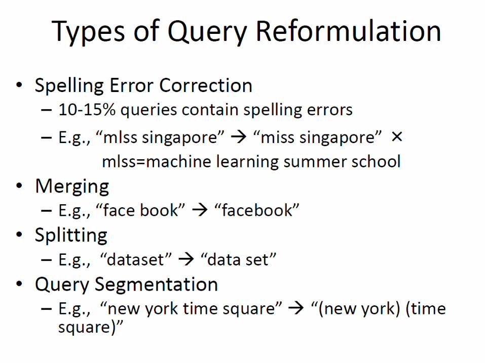
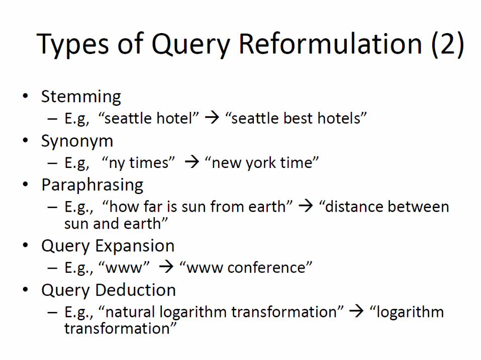
Outline

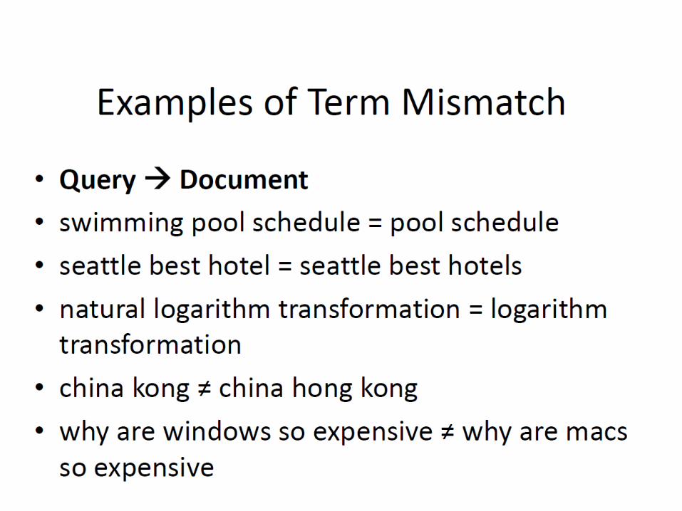
• Big Data Everywhere• Motivation (How Big Data solves Speller Issue)• The New Bottleneck in Big Data• Search Engine (Big Data)

– Query Document Mismatch– Query Reformulation

• Potential Solutions– How much of the data?

• Intelligent Sampling of Big Data

– How to clean up the data?• Filtering

• Conclusions

Big Data EveryWhere!

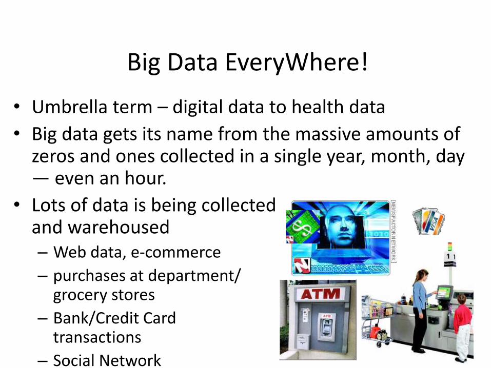
• Umbrella term – digital data to health data

• Big data gets its name from the massive amounts of zeros and ones collected in a single year, month, day — even an hour.

• Lots of data is being collected and warehoused – Web data, e-commerce

– purchases at department/grocery stores

– Bank/Credit Card transactions

– Social Network

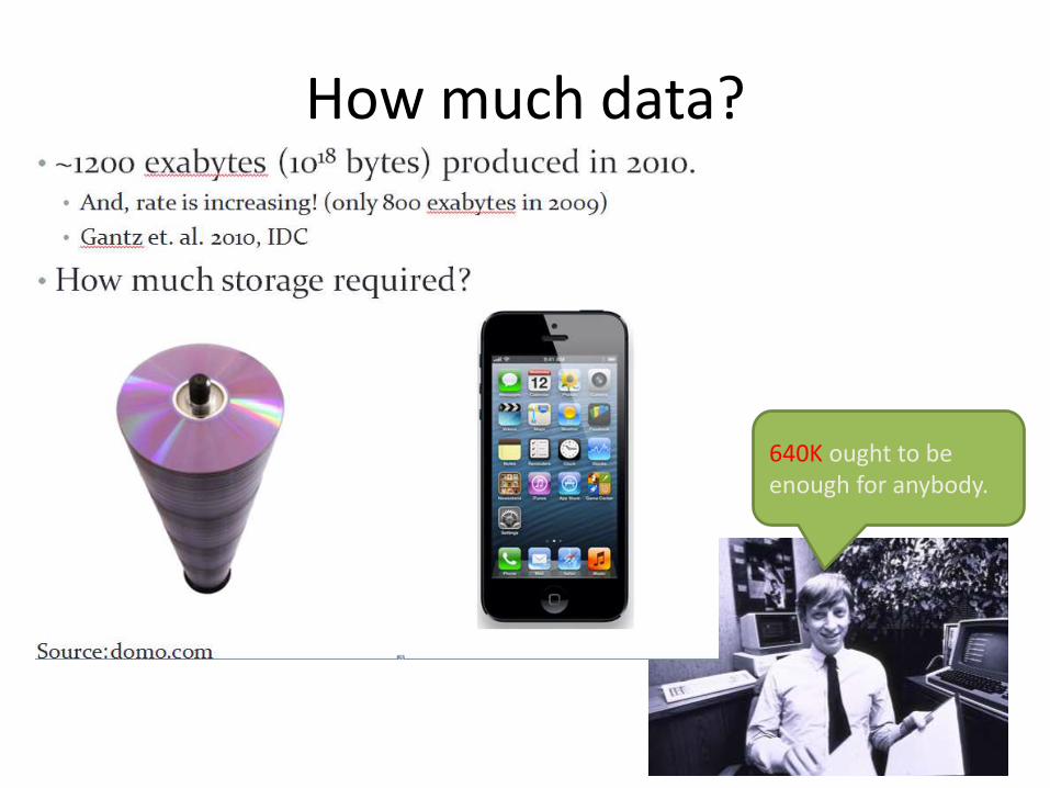
How much data?

640K ought to be enough for anybody.

Opportunities?

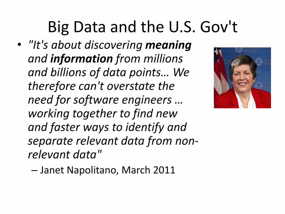
Big Data and the U.S. Gov't• "It's about discovering meaning

and information from millions and billions of data points… We therefore can't overstate the need for software engineers … working together to find new and faster ways to identify and separate relevant data from non-relevant data"– Janet Napolitano, March 2011

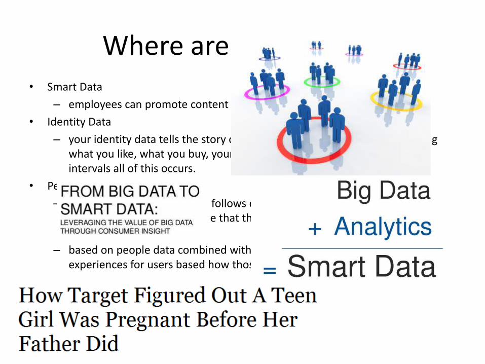
Where are we headed?• Smart Data

– employees can promote content targeting potential customers.

• Identity Data

– your identity data tells the story of who you are in the digital age, including what you like, what you buy, your lifestyle choices and at what time or intervals all of this occurs.

• People Data

– who your audience likes and follows on social media, what links they click, how long they stay on the site that they clicked over to and how many converted versus bounced.

– based on people data combined with on-site analytics, a site can customize experiences for users based how those customers want to use a site.

Big Data – How does it solve problems?

Motivating Example: Speller Problem Solved!

Speller

Google Speller

Microsoft Word Speller

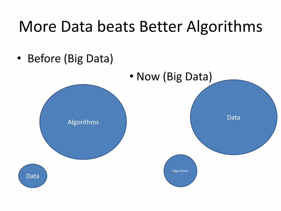
More Data beats Better Algorithms

• Before (Big Data)

• Now (Big Data)

Algorithms

Data

Data

Algorithms

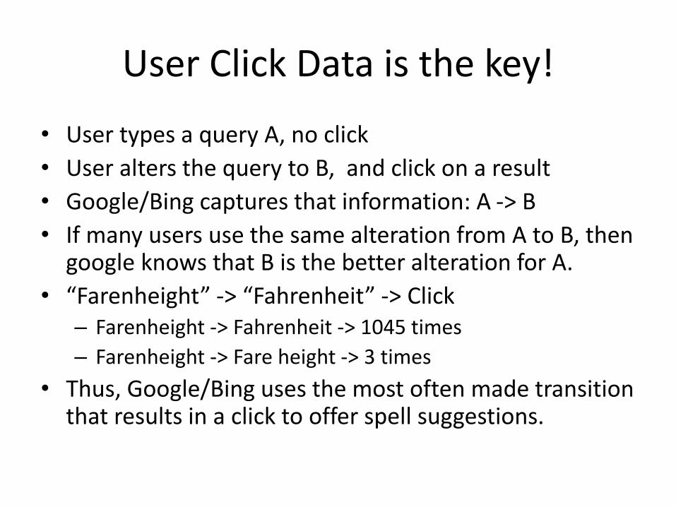
User Click Data is the key!

• User types a query A, no click

• User alters the query to B, and click on a result

• Google/Bing captures that information: A -> B

• If many users use the same alteration from A to B, then google knows that B is the better alteration for A.

• “Farenheight” -> “Fahrenheit” -> Click– Farenheight -> Fahrenheit -> 1045 times

– Farenheight -> Fare height -> 3 times

• Thus, Google/Bing uses the most often made transition that results in a click to offer spell suggestions.

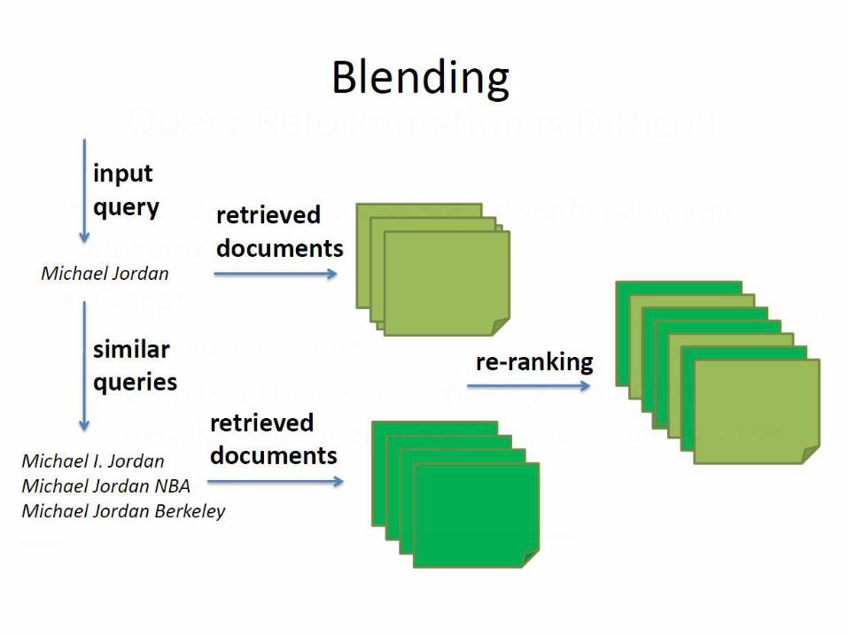
Other Search Engine Problems Solved using Big Data

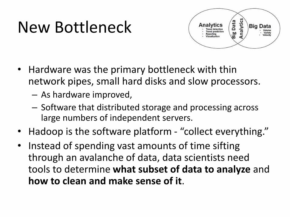
New Bottleneck

• Hardware was the primary bottleneck with thin network pipes, small hard disks and slow processors. – As hardware improved,

– Software that distributed storage and processing across large numbers of independent servers.

• Hadoop is the software platform - “collect everything.”

• Instead of spending vast amounts of time sifting through an avalanche of data, data scientists need tools to determine what subset of data to analyze and how to clean and make sense of it.

33

Motivation: Training a Neural Network

for Face Recognition

Neural Net MaleFemale

Training

M M M M M M M M M M

M M M M M M M M M M

M M M M M M M M M M

M M M M M M M M M M

F F F F F F F F F F

M M M M M M M M M M

34

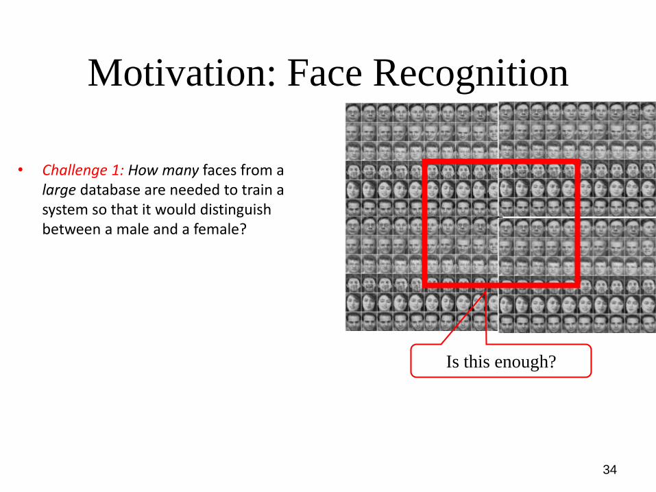
Motivation: Face Recognition

• Challenge 1: How many faces from a large database are needed to train a system so that it would distinguish between a male and a female?

Is this enough?

35

Motivation: Face Recognition

• Challenge 2: Predictive accuracy depends on the quality of data in the training set. Hence improving the quality of training data (i.e. handling noise) improves the accuracy over unseen instances.

Female

Female

Training Instance Class Label

Male

No n

ois

eF

eatu

re n

ois

eC

lass

nois

e

No

ise

36

The Curse of Large Datasets

There are two main challenges of dealing with large datasets.

• Running Time: Reducing the amount of time it takes for the mining algorithm to train.

• Predictive Accuracy: Poor quality of instances in training data lead to lower predictive accuracies. Large datasets are usually heterogeneous, and subjected to more noisy instances [Liu, MotodaDMKD 2002].

The goal of our work is to address these questions and provide some solutions.

37

Two Potential Solutions

• There are two potential solutions to the problems

• Running time:– Scale up existing data mining algorithms (for e.g.

parallelize them)

– Scale down the data

• Predictive accuracy:– Better mining algorithms

– Improve the quality of the training data

Intelligent Sampling

Bootstrapping We shall focus on first scaling down the data, while improving the quality

38

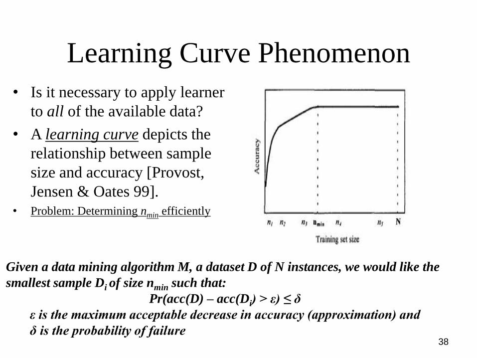
Learning Curve Phenomenon

• Is it necessary to apply learner

to all of the available data?

• A learning curve depicts the

relationship between sample

size and accuracy [Provost,

Jensen & Oates 99].

• Problem: Determining nmin efficiently

Given a data mining algorithm M, a dataset D of N instances, we would like the

smallest sample Di of size nmin such that:

Pr(acc(D) – acc(Di) > ε) ≤ δ

ε is the maximum acceptable decrease in accuracy (approximation) and

δ is the probability of failure

39

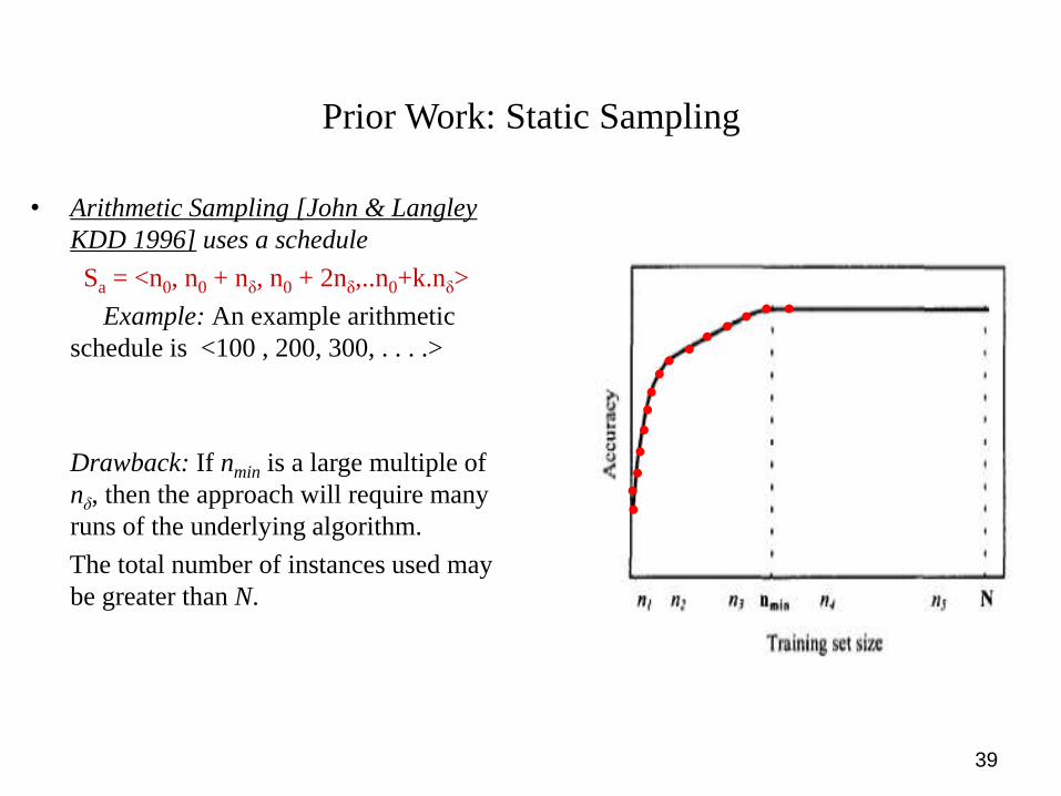
Prior Work: Static Sampling

• Arithmetic Sampling [John & Langley

KDD 1996] uses a schedule

Sa = <n0, n0 + nδ, n0 + 2nδ,..n0+k.nδ>

Example: An example arithmetic

schedule is <100 , 200, 300, . . . .>

Drawback: If nmin is a large multiple of

nδ, then the approach will require many

runs of the underlying algorithm.

The total number of instances used may

be greater than N.

40

Prior Work in Progressive Sampling

• Geometric Sampling [Provost, Jenson &

Oates KDD 1999] uses a schedule

Sg= <n0, a.n0,a2.n0, ………,ak.n0>

An example geometric schedule is:

<100,200,400,800, . . .>

Drawbacks:

(a) In practice, Geometric Sampling

suffers from overshooting nmin.

(b) Not dependent on the dataset at

hand. A good sampling algorithm

is expected to have low bias and

low sampling variance

For example in the KDD CUP dataset,

when nmin=56,600,

the geometric schedule is as follows:

{100, 200, 400, 800, 1600, 3200, 6400,

12800, 25600, 51200, 102400}.

Notice here that the last sample has

overshot nmin by 45,800 instances

Intelligent Dynamic Adaptive Sampling

(a) Sampling schedule → adaptive

to the dataset under consideration.

(c) Adaptive stopping criterion to

determine when the learning curve

has reached a point of diminishing

returns.

42

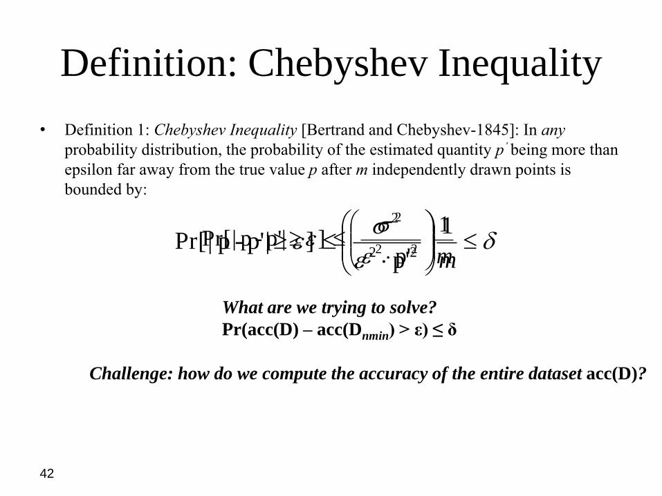
Definition: Chebyshev Inequality

• Definition 1: Chebyshev Inequality [Bertrand and Chebyshev-1845]: In any

probability distribution, the probability of the estimated quantity p’ being more than

epsilon far away from the true value p after m independently drawn points is

bounded by:

m

1

p' ] |p' -p| Pr[

22

2

m

1

p' ] |p' -p| Pr[

22

2

What are we trying to solve?

Pr(acc(D) – acc(Dnmin) > ε) ≤ δ

Challenge: how do we compute the accuracy of the entire dataset acc(D)?

Myopic Strategy: One Step at a time

43

û(Di)

û(Di+1)

||

1

)(||

1)

iû(D

iD

i

i

i

xfD

[Average over the sample Di]

The instance function f(xi) used here is a

Bernoulli trial, 0-1 classification accuracy

44

m

1

p' ] |p' -p| Pr[

22

2

True value

u(Da)-u(Db);

where |Da|>|Db|>nmin

Estimated value

u(Da)-u(Db);

where |Da|>|Db|≥1

Plateau Region:

p=0

Myopic Strategy:

u(Di) - u(Di-1)

m

BOOT 1

))u(D-)u(D( )u(D-)u(D -0 Pr

2

1-ii

2

2

1-ii

1

))u(D-)u(D(

2

1-ii

2

2

BOOTm

m

BOOT 1

))u(D-)u(D( 2

1-ii

2

2

Approximation parameterConfidence parameter

Bootstrapped Variance p’(to improve the quality of the training data)

45

Four Possible cases for Convergence

Negative False1

p' and |p' -p| (d)

Positive False 1

p' and |p' -p| (c)

instances more Add1

p' and |p' -p| (b)

Converged1

p' and |p' -p| (a)

22

2

22

2

22

2

22

2

m

m

m

m

46

47

Empirical Results

• (Full): SN = <N>, a single sample with all the instances. This is the most commonlyused method. This method suffers from both speed and memory drawbacks.

• (Geo): Geometric Sampling, in which the training set size is increasedgeometrically, Sg = <|D1|,a.|D1|,a

2.|D1|,a3.|D1|….ak.|D1|> until convergence is

reached. In our experiments, we use |D1|=100, and a=2 as per the Provost et’ alstudy.

• (IDASA): Our adaptive sampling approach using Chebyshev Bounds. We use ε =0.001 and δ = 0.05 (95% probability) in all our experiments.

• (Oracle): So = <nmin>, the optimal schedule determined by an omniscient oracle; wedetermined nmin empirically by analyzing the full learning curve beforehand. We usethese results to empirically compare the optimum performance with other methods.

• We compare these methods using the following two performance criteria:

• (a) The mean computation time: Averaged over 20 runs for each dataset.

• (b) The total number of instances needed to converge: If the sampling schedule, isas follows: S={|D1|,|D2|,|D3|….|Dk|}, then the total number of instances would be|D1|+|D2|+|D3|….+|Dk|.

48

Empirical Results (for Non-incremental Learner)

49

Empirical Results (for Incremental Learners)

Table 2: Comparison of the mean computation time required for convergence by the different methods to obtain the same accuracy. Time

is in CPU seconds (by the linux time command)

Table 1: Comparison of the total number of instances required for convergence by the different methods to obtain the same accuracy

50

Conclusions

1) Big data is evolving and Smart data, Identity data and People data are here to stay. Think of them as the human discovery of fire, the wheel and wheat.

2) Search Engines use Big Data for their relevance and ranking problems3) Main Bottleneck: data scientists need tools to determine what subset of data to

analyze and how to clean and make sense of it4) Intelligent Sampling addresses what subset to use.5) Bootstrap filtering helps clean up the data.6) In conclusion, Big data is big and it is here to stay. And it’s only getting bigger!!

51

Questions & Suggestions

Filtering

53

Bayesian Analysis of Ensemble Filtering

L1(k-NN Classifier)

Training Data

D

L3(Linear Machine)L2(Decision Tree)

θ1

θ3

θ2θ1 δ(yj , θ1(xj))θ2 δ(yj , θ2(xj))θ3 δ(yj , θ3(xj))

=1 if θ.(xj) is the same as

the true label yj else 0

( xj , yj )

54

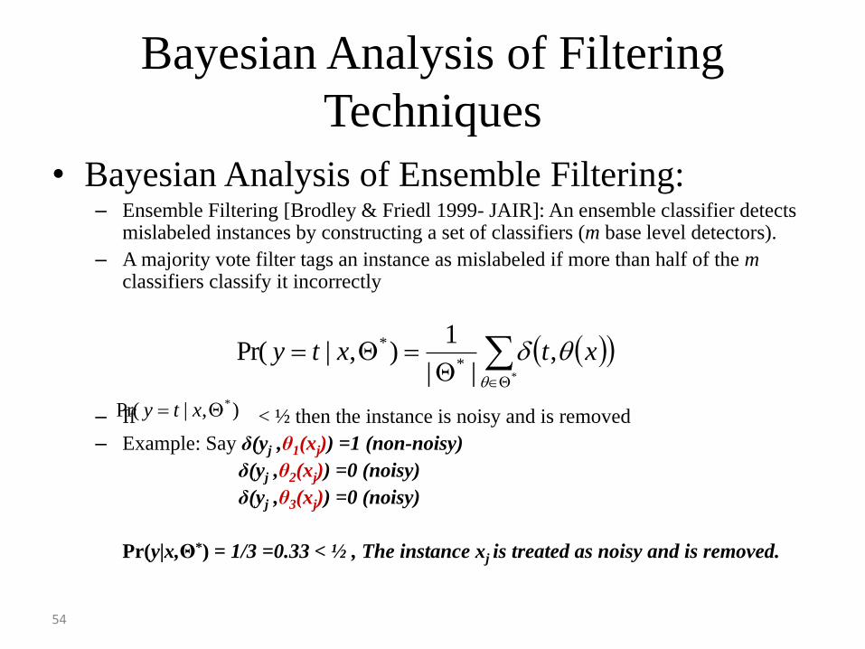
Bayesian Analysis of Filtering

Techniques

• Bayesian Analysis of Ensemble Filtering:– Ensemble Filtering [Brodley & Friedl 1999- JAIR]: An ensemble classifier detects

mislabeled instances by constructing a set of classifiers (m base level detectors).

– A majority vote filter tags an instance as mislabeled if more than half of the mclassifiers classify it incorrectly

– If < ½ then the instance is noisy and is removed

– Example: Say δ(yj ,θ1(xj)) =1 (non-noisy)

δ(yj ,θ2(xj)) =0 (noisy)

δ(yj ,θ3(xj)) =0 (noisy)

Pr(y|x,Θ*) = 1/3 =0.33 < ½ , The instance xj is treated as noisy and is removed.

*

,||

1),|Pr(

*

*

xtxty

),|Pr( * xty

55

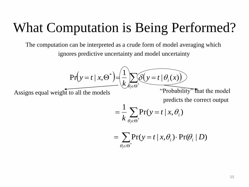
What Computation is Being Performed?

*

)(|1

,|Pr *

i

xtyk

xty i

) , |Pr(1

*

ixtyk

i

The computation can be interpreted as a crude form of model averaging which

ignores predictive uncertainty and model uncertainty

)|Pr(), |Pr(*

Dxty ii

i

Assigns equal weight to all the models “Probability” that the model

predicts the correct output

56

Bootstrapped Model Averaging

– Now that we know what computation is occurring in the filtering techniques, we now propose using a better approximation to model averaging.

– There are lots of model averaging approaches, we choose this because it is efficient for large datasets.

– This particular case uses Efron’s non-parametric bootstrapping approach which is as shown below:

where the datasets D’ are the different bootstrap samples generated from the original dataset D.

DDxyxyDLD

i

i

|'Pr,|Pr ,|Pr)'(,'

57

Introduction to Bootstrapping

• Basic idea:

– Draw datasets by sampling with replacement from the original dataset

– Each perturbed dataset has the same size as the original training set

D

Db’

D2’

D1’

58

Bootstrap Averaging

D

Db’

D2’

D1’

L(Decision Tree)

θ1

θ2

θb

59

Bootstrapped Model Averaging (BMA) vs Filtering

• We now try using bootstrapped model averaging and compare it with partition filtering (10 folds). We used 80% training set and a fixed 20% for testing. We eliminate noisy instances as in partition filtering, and obtained the following results:

• Thus we see can conclude that bootstrap averaged model produces a better approximation to model averaging when compared to the model averaging performed by filtering. 2500 instances -> 10% noise – 250 noisy instances

Partition filtering removed – 194 instances (162 instances were actually noisy, 32 instances were good ones)

BMA filtering removed – 189 instances (178 instances were noisy, 11 instances were non-noisy)

Overlap of noisy instances between the two techniques = 151 instances

LED24 Dataset

60

Why remove noise?• 1) Removing noisy instances increases

the predictive accuracy. This has been

shown by Quinlan [Qui86] and Brodley

and Friedl ([BF96][BF99])

• 2) Removing noisy instances creates a

simpler model. We show this empirically

in the Table.

• 3) Removing noisy instances reduces the

variance of the predictive accuracy: This

makes a more stable learner whose

accuracy estimate is more likely to be the

true value.

61

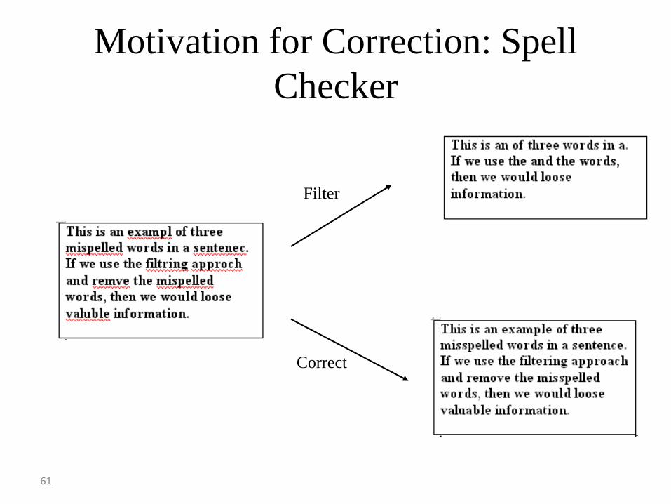
Motivation for Correction: Spell

Checker

Filter

Correct

62

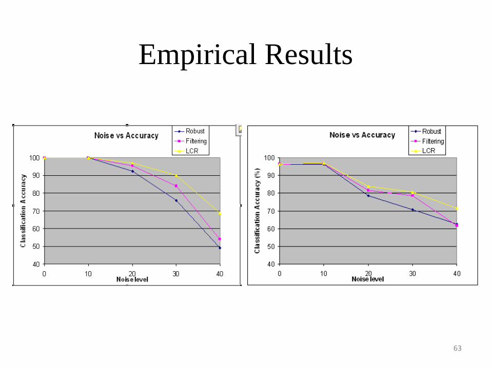
Empirical Comparison of Noise Handling Techniques

• We compare the following approaches for noise handling:– Robust Algorithms: To avoid overfitting, post pruning

and stop conditions are used that prevent further splitting of a leaf node.

– Partition Filtering: Discards instances that the C4.5 decision tree misclassifies, and builds a new tree using the remaining data

– LC Approach: Corrects instances that the C4.5 decision tree misclassified and built a new tree using the corrected data.

63

Empirical Results

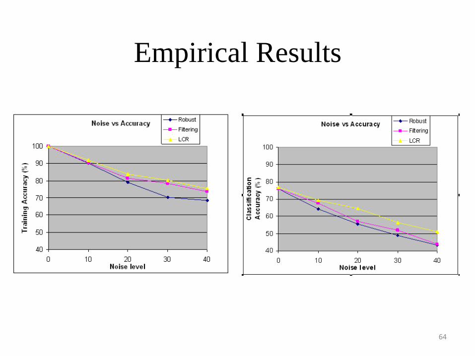
64

Empirical Results

Conclusion

65

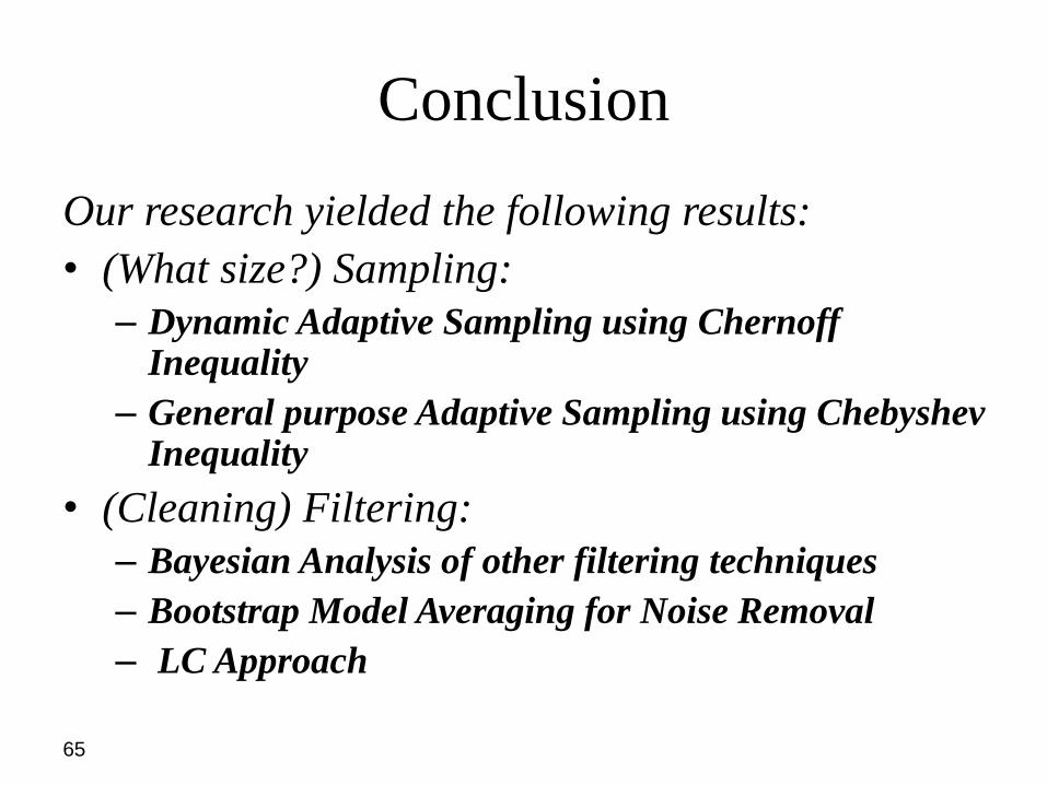
Our research yielded the following results:

• (What size?) Sampling:

– Dynamic Adaptive Sampling using ChernoffInequality

– General purpose Adaptive Sampling using ChebyshevInequality

• (Cleaning) Filtering:

– Bayesian Analysis of other filtering techniques

– Bootstrap Model Averaging for Noise Removal

– LC Approach

66

Questions & Suggestions