big data - lecture 3 supervised classification · introduction naive bayes classi er nearest...
TRANSCRIPT

IntroductionNaive Bayes classifier
Nearest Neighbour ruleSVM
Big Data - Lecture 3Supervised classification
S. Gadat
Toulouse, Novembre 2014
S. Gadat Big Data - Lecture 3
IntroductionNaive Bayes classifier
Nearest Neighbour ruleSVM
Big Data - Lecture 3Supervised classification
S. Gadat
Toulouse, Novembre 2014
S. Gadat Big Data - Lecture 3

IntroductionNaive Bayes classifier
Nearest Neighbour ruleSVM
I - 2 Binary supervised classificationI - 3 Statistical model
Schedule
1 IntroductionI - 1 MotivationsI - 2 Binary supervised classificationI - 3 Statistical model
2 Naive Bayes classifierII - 1 Posterior distributionII - 2 Naive Bayes classifiers in one slideII - 3 Back to the exampleII - 4 General featuresII - 5 A real-world example: spam filtering
3 Nearest Neighbour ruleIII - I A very standard classification algorithmIII - 2 Statistical frameworkIII - 3 Margin assumptionIII - 4 Classification abilitiesIII - 5 Short example
4 Support Vector MachinesMotivation
S. Gadat Big Data - Lecture 3

IntroductionNaive Bayes classifier
Nearest Neighbour ruleSVM
I - 2 Binary supervised classificationI - 3 Statistical model
I - 1 Motivations: Pattern recognition - Medical diagnosisProblem: Automatic classification of handwritten digits, Mnist US Postals database
Source: Y. LeCun, L. Bottou, Y. Bengio, and P. Haffner. ”Gradient-based learning applied todocument recognition.” Proc. of the IEEE, 86(11):2278-2324, Nov. 1998.
New observation Automatic prediction of the class? New diagnosis Nouveau diagnostic?Statistical Approach:
Dataset digital recording (24× 24 pixels) ↪→ described over {0, . . . , 255}24×24.
Medical tests and personal informations (Age, gender, weight, . . . ,)
Collect n samples of observations in the learning set: Dn := (X1, Y1), . . . , (Xn, Yn),Build a prediction from Dn, denoted Φn (”number” / ”healthy” vs ”diseased”).We observe a new X, behaviour of Φn(X) with a large number of observations?
S. Gadat Big Data - Lecture 3

IntroductionNaive Bayes classifier
Nearest Neighbour ruleSVM
I - 2 Binary supervised classificationI - 3 Statistical model
I - 1 Motivation: Spam Detection (Corpus classification)Probleme: Spam Detection, Hp Database
New observation: automatic prediction of the class?Statistical approach:
Description of the messages with a preliminary dictionary of p typical words.
Statistics, Probability, $, !,. . .
Store n samples of Np × {0, 1}: Dn := (X1, Y1), . . . , (Xn, Yn).
Build a classifier / predictor / algorithm from Dn denoted Φn to predict ”Spam” vs ”nonSpam”.
A new message X enters the mailbox, predict Φn(X) with a large number of samples?
S. Gadat Big Data - Lecture 3

IntroductionNaive Bayes classifier
Nearest Neighbour ruleSVM
I - 2 Binary supervised classificationI - 3 Statistical model
I - 2 Binary supervised classification
We observe a learning set Dn of Rd × {0, 1}.
Compute a classifier Φn from Dn (’off-line’ algorithm).
Aim: quantify the prediction ability of each algorithms through a cost function `
Many application fields
Signal and image processing
Text classification
Bioinformatics
Credit scoring
S. Gadat Big Data - Lecture 3

IntroductionNaive Bayes classifier
Nearest Neighbour ruleSVM
I - 2 Binary supervised classificationI - 3 Statistical model
I - 3 Different statistical model (almost equivalent)
Classification model (simplest)
We observe n samples i.i.d. (X1, Y1), . . . (Xn, Yn).
Positions X and labels Y are described through the joint law: (X,Y ) ∼ P .
X is a random vector in a compact set K ⊂ Rd and Y ∈ {0, 1}.The marginal law PY follows a Bernoulli distribution (balanced B(1/2)).
Conditional laws: a.c. w.r.t. dλK(.), f (resp. g) density of X|Y = 0 (resp. X|Y = 1).
Discriminant analysis (not so simple)
We observe n/2 samples of f : (X1, . . . , Xn/2) and (Y1, . . . , Yn/2) = (0, . . . , 0).
We observe n/2 samples of g: (Xn/2+1, . . . , Xn) and (Y1, . . . , Yn/2) = (1, . . . , 1).
In each situation, the important tool is the regression function:
η(x) =g(x)
f(x) + g(x)= P(Y = 1|X).
S. Gadat Big Data - Lecture 3

IntroductionNaive Bayes classifier
Nearest Neighbour ruleSVM
I - 2 Binary supervised classificationI - 3 Statistical model
I - 3 Different statistical model (almost equivalent)
Classification model (simplest)
An algorithm Φ is a function of X and “predict” 0 or 1.
The risk of the algorithm Φ is defined as
R(Φ) = P [Φ(X) 6= Y ] = EP[1Φ(X)6=Y
]There exists an optimal classifier: the Bayes rule
ΦBayes(X) := 1η(X)≥1/2.
Discriminant analysis (not so simple) Omitted here.
Theoreme (Gyorfi ’78, Mammen & Tsybakov ’99)
For any classifier Φ, the excess risk satisfies
R(Φ)−R(ΦBayes) = EPX[|2η(X)− 1| 1Φ(X) 6=ΦBayes(X)
]Since P is unknown in pratique, ΦBayes is intractable.
S. Gadat Big Data - Lecture 3

IntroductionNaive Bayes classifier
Nearest Neighbour ruleSVM
II - 1 Posterior distributionII - 2 Naive Bayes classifiers in one slideII - 3 Back to the exampleII - 4 General featuresII - 5 A real-world example: spam filtering
Schedule
1 IntroductionI - 1 MotivationsI - 2 Binary supervised classificationI - 3 Statistical model
2 Naive Bayes classifierII - 1 Posterior distributionII - 2 Naive Bayes classifiers in one slideII - 3 Back to the exampleII - 4 General featuresII - 5 A real-world example: spam filtering
3 Nearest Neighbour ruleIII - I A very standard classification algorithmIII - 2 Statistical frameworkIII - 3 Margin assumptionIII - 4 Classification abilitiesIII - 5 Short example
4 Support Vector MachinesMotivation
S. Gadat Big Data - Lecture 3

IntroductionNaive Bayes classifier
Nearest Neighbour ruleSVM
II - 1 Posterior distributionII - 2 Naive Bayes classifiers in one slideII - 3 Back to the exampleII - 4 General featuresII - 5 A real-world example: spam filtering
A bit of intuition
A particular example
G(ender) H(eight) (m) W(eight) (kg) F(oot size) (cm)
M 1.82 82 30M 1.80 86 28M 1.70 77 30M 1.80 75 25F 1.52 45 15F 1.65 68 20F 1.68 59 18F 1.75 68 23
Is (1.81, 59, 21) male of female?
S. Gadat Big Data - Lecture 3

IntroductionNaive Bayes classifier
Nearest Neighbour ruleSVM
II - 1 Posterior distributionII - 2 Naive Bayes classifiers in one slideII - 3 Back to the exampleII - 4 General featuresII - 5 A real-world example: spam filtering
Bayesian probabilities
Question: P (G = M | (H,W,F ) = (1.81, 59, 21)) >P (G = F | (H,W,F ) = (1.81, 59, 21))?
Bayes law:
P(G|H,W,F ) =P(G)× P(H,W,F |S)
P(H,W,F )
In other words:
posterior =prior× likelihood
evidence
But P(H,W,F ) does not depend on G, so the question boils down to:
P(G = M)× P(H,W,F |G = M) > P(G = F )× P(H,W,F |G = F )?
Naive Bayes rule aims to mimic this former decision:
1 Estimate the conditional probabilities
Pn(M)× Pn(H,W,F |G = M) and Pn(F )× Pn(H,W,F |G = F )
2 Φn: decide M or F according to the ranks of the products above.
P(G) is easy to estimate. What about P(H,W,F |G)?
S. Gadat Big Data - Lecture 3

IntroductionNaive Bayes classifier
Nearest Neighbour ruleSVM
II - 1 Posterior distributionII - 2 Naive Bayes classifiers in one slideII - 3 Back to the exampleII - 4 General featuresII - 5 A real-world example: spam filtering
Naive Bayes hypothesis
Discretize range(H) in 10 segments.→ P(H,W,F |G) is a 3-dimensional array.
→ 103 values to estimate→ requires lots of data!
Curse of dimensionality: #(data) scales exponentially with #(features).
Reminder, conditional probabilities:
P(H,W,F |G) = P(H|G)× P(W |G,H)× P(F |G,H,W )
Naive Bayes: “what if
{P(W |G,H) = P(W |G)
P(F |G,H,W ) = P(F |G)?”
→ Then P(H,W,F |G) = P(H|G)× P(W |G)× P(F |G)→ only 3× 10 values to estimate
S. Gadat Big Data - Lecture 3
IntroductionNaive Bayes classifier
Nearest Neighbour ruleSVM
II - 1 Posterior distributionII - 2 Naive Bayes classifiers in one slideII - 3 Back to the exampleII - 4 General featuresII - 5 A real-world example: spam filtering
Naive Bayes hypothesis, cont’d
P(W |S,H) = P(W |S) what does that mean?“Among male individuals, the weight is independent of the height”
What do you think?
Despite that naive assumption, Naive Bayes classifiers perform very well!
Let’s formalize that a little more.
S. Gadat Big Data - Lecture 3

IntroductionNaive Bayes classifier
Nearest Neighbour ruleSVM
II - 1 Posterior distributionII - 2 Naive Bayes classifiers in one slideII - 3 Back to the exampleII - 4 General featuresII - 5 A real-world example: spam filtering
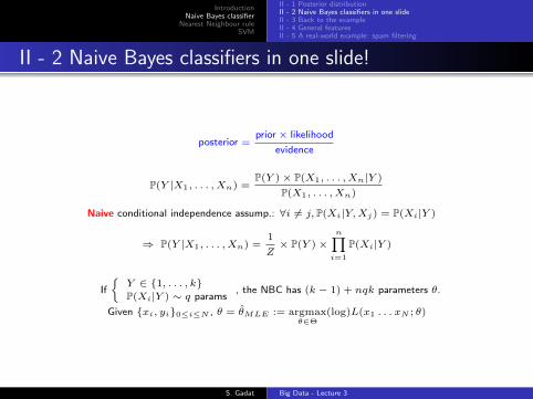
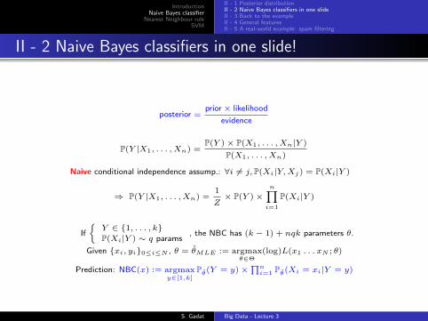
II - 2 Naive Bayes classifiers in one slide!
posterior =prior× likelihood
evidence
P(Y |X1, . . . , Xn) =P(Y )× P(X1, . . . , Xn|Y )
P(X1, . . . , Xn)
Naive conditional independence assump.: ∀i 6= j, P(Xi|Y,Xj) = P(Xi|Y )
⇒ P(Y |X1, . . . , Xn) =1
Z× P(Y )×
n∏i=1
P(Xi|Y )
If
{Y ∈ {1, . . . , k}P(Xi|Y ) ∼ q params
, the NBC has (k − 1) + nqk parameters θ.
Given {xi, yi}0≤i≤N , θ = θMLE := argmaxθ∈Θ
(log)L(x1 . . . xN ; θ)
Prediction: NBC(x) := argmaxy∈[1,k]
Pθ(Y = y)×∏ni=1 Pθ(Xi = xi|Y = y)
S. Gadat Big Data - Lecture 3

IntroductionNaive Bayes classifier
Nearest Neighbour ruleSVM
II - 1 Posterior distributionII - 2 Naive Bayes classifiers in one slideII - 3 Back to the exampleII - 4 General featuresII - 5 A real-world example: spam filtering
II - 2 Naive Bayes classifiers in one slide!
posterior =prior× likelihood
evidence
P(Y |X1, . . . , Xn) =P(Y )× P(X1, . . . , Xn|Y )
P(X1, . . . , Xn)
Naive conditional independence assump.: ∀i 6= j, P(Xi|Y,Xj) = P(Xi|Y )
⇒ P(Y |X1, . . . , Xn) =1
Z× P(Y )×
n∏i=1
P(Xi|Y )
If
{Y ∈ {1, . . . , k}P(Xi|Y ) ∼ q params
, the NBC has (k − 1) + nqk parameters θ.
Given {xi, yi}0≤i≤N , θ = θMLE := argmaxθ∈Θ
(log)L(x1 . . . xN ; θ)
Prediction: NBC(x) := argmaxy∈[1,k]
Pθ(Y = y)×∏ni=1 Pθ(Xi = xi|Y = y)
S. Gadat Big Data - Lecture 3

IntroductionNaive Bayes classifier
Nearest Neighbour ruleSVM
II - 1 Posterior distributionII - 2 Naive Bayes classifiers in one slideII - 3 Back to the exampleII - 4 General featuresII - 5 A real-world example: spam filtering
II - 3 Back to the example
P(G|H,W,F ) =1
Z× P(G)× P(H|G)× P(W |G)× P(F |G)
S(ex) H(eight) (m) W(eight) (kg) F(oot size) (cm)
M 1.82 82 30M 1.80 86 28M 1.70 77 30M 1.80 75 25F 1.52 45 15F 1.65 68 20F 1.68 59 18F 1.75 68 23
P(S = M) =?
P(H = 1.81|S = M) =?
P(W = 59|S = M) =?
P(F = 21|S = M) =?
S. Gadat Big Data - Lecture 3

IntroductionNaive Bayes classifier
Nearest Neighbour ruleSVM
II - 1 Posterior distributionII - 2 Naive Bayes classifiers in one slideII - 3 Back to the exampleII - 4 General featuresII - 5 A real-world example: spam filtering
II - 3 Back to the example
P(G|H,W,F ) =1
Z× P(G)× P(H|G)× P(W |G)× P(F |G)
> gens <- read.table("sex classif.csv", sep=";", colnames)> library("MASS")> fitdistr(gens[1:4,2],"normal")...> 0.5*dnorm(1.81,mean=1.78,sd=0.04690416)
*dnorm(59,mean=80,sd=4.301163)*dnorm(21,mean=28.25,sd=2.0463382)
> 0.5*dnorm(1.81,mean=1.65,sd=0.08336666)*dnorm(59,mean=60,sd=9.407444)*dnorm(21,mean=19,sd=2.915476)
S. Gadat Big Data - Lecture 3

IntroductionNaive Bayes classifier
Nearest Neighbour ruleSVM
II - 1 Posterior distributionII - 2 Naive Bayes classifiers in one slideII - 3 Back to the exampleII - 4 General featuresII - 5 A real-world example: spam filtering
II - 3 Back to the example
P(G|H,W,F ) =1
Z× P(G)× P(H|G)× P(W |G)× P(F |G)
S is discrete, H, W and F are assumed Gaussian.S pS µH|S σH|S µW |S σW |S µF |S σF |SM 0.5 1.78 0.0469 80 4.3012 28.25 2.0463F 0.5 1.65 0.0834 60 9.4074 19 2.9154
P(M |1.81, 59, 21) =1
Z× 0.5×
e−(1.78−1.81)2
2·0.04692
√2π0.04692
×e−(80−59)2
2·4.30122
√2π4.30122
×e−(28.25−21)2
2·2.04632
√2π2.04632
=1
Z× 7.854 · 10
−10
P(F |1.81, 59, 21) =1
Z× 0.5×
e−(1.65−1.81)2
2·0.08342
√2π0.08342
×e−(60−59)2
2·9.40742
√2π9.40742
×e−(19−21)2
2·2.91542
√2π2.91542
=1
Z× 1.730 · 10
−3
S. Gadat Big Data - Lecture 3

IntroductionNaive Bayes classifier
Nearest Neighbour ruleSVM
II - 1 Posterior distributionII - 2 Naive Bayes classifiers in one slideII - 3 Back to the exampleII - 4 General featuresII - 5 A real-world example: spam filtering
II - 3 Back to the example
P(G|H,W,F ) =1
Z× P(G)× P(H|G)× P(W |G)× P(F |G)
Conclusion: given the data, (1.81m, 59kg, 21cm) is more likely to be female.
S. Gadat Big Data - Lecture 3
IntroductionNaive Bayes classifier
Nearest Neighbour ruleSVM
II - 1 Posterior distributionII - 2 Naive Bayes classifiers in one slideII - 3 Back to the exampleII - 4 General featuresII - 5 A real-world example: spam filtering
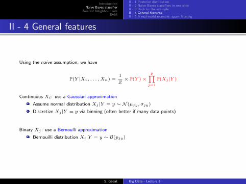
II - 4 General features
Using the naive assumption, we have
P(Y |X1, . . . , Xn) =1
Z× P(Y )×
p∏j=1
P(Xj |Y )
Continuous Xi: use a Gaussian approximation
Assume normal distribution Xj |Y = y ∼ N (µjy, σjy)
Discretize Xj |Y = y via binning (often better if many data points)
Binary Xj : use a Bernoulli approximation
Bernouilli distribution Xi|Y = y ∼ B(pjy)
S. Gadat Big Data - Lecture 3

IntroductionNaive Bayes classifier
Nearest Neighbour ruleSVM
II - 1 Posterior distributionII - 2 Naive Bayes classifiers in one slideII - 3 Back to the exampleII - 4 General featuresII - 5 A real-world example: spam filtering
Algorithm
Train:For all possible values of Y and Xj ,
compute Pn(Y = y) and Pn(Xj = xj |Y = y).
Predict:Given (x1, . . . , xp), return y that
maximizes P(Y = y)∏pj=1 Pn(Xj = xj |Y = y).
S. Gadat Big Data - Lecture 3

IntroductionNaive Bayes classifier
Nearest Neighbour ruleSVM
II - 1 Posterior distributionII - 2 Naive Bayes classifiers in one slideII - 3 Back to the exampleII - 4 General featuresII - 5 A real-world example: spam filtering
When should you use NBC?
Needs little data to estimate parameters.
Can easily deal with large feature spaces.
Requires little tuning (but a bit of feature engineering).
Without good tuning, more complex approaches are often outperformed by NBC.
. . . despite the naive independence assumption!
If you want to understand why: The Optimality of Naive Bayes, H. Zhang, FLAIRS, 2004.
S. Gadat Big Data - Lecture 3

IntroductionNaive Bayes classifier
Nearest Neighbour ruleSVM
II - 1 Posterior distributionII - 2 Naive Bayes classifiers in one slideII - 3 Back to the exampleII - 4 General featuresII - 5 A real-world example: spam filtering
A little more
Computational amendments:
Never say never!
P(Y = y|Xj = xj , j ∈ [1, p]) =1
ZP(Y = y)×
p∏j=1
P(Xj = xj |Y = y)
But if P(Xj = xj |Y = y) = 0, then all other info from Xj is lost!→ never set a probability estimate below ε (sample correction)
Additive model
Log-likelihood: log P(Y |X) = − logZ + log P(Y ) +p∑j=1
log P(Xj |Y ) and:
logP(Y |X)
P(Y |X)= log
(P(Y )
1− P(Y )
)+
p∑j=1
log
(P(Xj |Y )
P(Xj |Y )
)
= α+
n∑j=1
g(Xj)
S. Gadat Big Data - Lecture 3

IntroductionNaive Bayes classifier
Nearest Neighbour ruleSVM
II - 1 Posterior distributionII - 2 Naive Bayes classifiers in one slideII - 3 Back to the exampleII - 4 General featuresII - 5 A real-world example: spam filtering
II - 5 A real-world example: spam filtering
Build a NBC that classifies emails as spam/non-spam,using the occurence of words.
Any ideas?
S. Gadat Big Data - Lecture 3

IntroductionNaive Bayes classifier
Nearest Neighbour ruleSVM
II - 1 Posterior distributionII - 2 Naive Bayes classifiers in one slideII - 3 Back to the exampleII - 4 General featuresII - 5 A real-world example: spam filtering
The data
Data = a bunch of emails, labels as spam/non-spam.The Ling-spam dataset: http://csmining.org/index.php/ling-spam-datasets.html.
PreprocessingForm each email, remove:
stop-words
lemmatization
non-words
S. Gadat Big Data - Lecture 3

IntroductionNaive Bayes classifier
Nearest Neighbour ruleSVM
II - 1 Posterior distributionII - 2 Naive Bayes classifiers in one slideII - 3 Back to the exampleII - 4 General featuresII - 5 A real-world example: spam filtering
The data
Before:Subject: Re: 5.1344 Native speaker intuitions
The discussion on native speaker intuitions has been extremely
interesting, but I worry that my brief intervention may have
muddied the waters. I take it that there are a number of
separable issues. The first is the extent to which a native
speaker is likely to judge a lexical string as grammatical
or ungrammatical per se. The second is concerned with the
relationships between syntax and interpretation (although even
here the distinction may not be entirely clear cut).After:
re native speaker intuition discussion native speaker intuition
extremely interest worry brief intervention muddy waters number
separable issue first extent native speaker likely judge
lexical string grammatical ungrammatical per se second concern
relationship between syntax interpretation although even here
distinction entirely clear cut
S. Gadat Big Data - Lecture 3

IntroductionNaive Bayes classifier
Nearest Neighbour ruleSVM
II - 1 Posterior distributionII - 2 Naive Bayes classifiers in one slideII - 3 Back to the exampleII - 4 General featuresII - 5 A real-world example: spam filtering
The data
Keep a dictionnary V of the |V | most frequent words.
Count the occurence of each dictionary word in each example email.
m emails
ni words in email i
|V | words in dictionary
What is Y ?
What are the Xi?
S. Gadat Big Data - Lecture 3

IntroductionNaive Bayes classifier
Nearest Neighbour ruleSVM
II - 1 Posterior distributionII - 2 Naive Bayes classifiers in one slideII - 3 Back to the exampleII - 4 General featuresII - 5 A real-world example: spam filtering
Text classification features
Y = 1 if the email is a spam.
Xk = 1 if word i of dictionary appears in the email
Estimator of P(Xk = 1|Y = y):
xij is the jth word of email i, yi is the label of email i.
φky =
m∑i=1
ni∑j=1
1{xij=k and yi=y} + 1
m∑i=1
1{yi=y}ni + |V |
S. Gadat Big Data - Lecture 3

IntroductionNaive Bayes classifier
Nearest Neighbour ruleSVM
II - 1 Posterior distributionII - 2 Naive Bayes classifiers in one slideII - 3 Back to the exampleII - 4 General featuresII - 5 A real-world example: spam filtering
Getting started in R
> trainingSet <- read.table("emails-train-features.txt", sep=" ",
col.names=c("document","word","count"))
> labelSet <- read.table("emails-train-labels.txt", sep=" ",
col.names=c("spam"))
> num.features <- 2500
> doc.word.train <- spMatrix(max(trainingSet[,1]), num.features,
as.vector(trainingSet[,1]), as.vector(trainingSet[,2]),
as.vector(trainingSet[,3]))
> doc.class.train <- labelSet[,1]
> source("trainSpamClassifier") # your very own classifier!
> params <- trainSpamClassifier(doc.word.train,doc.class.train)
> testingSet <- read.table("emails-test-features.txt", sep=" ",
col.names=c("document","word","count"))
> doc.word.test <- spMatrix(max(testingSet[,1]), num.features,
as.vector(testingSet[,1]), as.vector(testingSet[,2]),
as.vector(testingSet[,3]))
> source("testSpamClassifier.r")
> prediction <- testSpamClassifier(params, doc.word.test) # does it workwell?
S. Gadat Big Data - Lecture 3

IntroductionNaive Bayes classifier
Nearest Neighbour ruleSVM
II - 1 Posterior distributionII - 2 Naive Bayes classifiers in one slideII - 3 Back to the exampleII - 4 General featuresII - 5 A real-world example: spam filtering
Going further in text mining in R
The “Text Mining” package:http://cran.r-project.org/web/packages/tm/http://tm.r-forge.r-project.org/
Useful if you want to change the features on the previous dataset.
S. Gadat Big Data - Lecture 3

IntroductionNaive Bayes classifier
Nearest Neighbour ruleSVM
III - I A very standard classification algorithmIII - 2 Statistical frameworkIII - 3 Margin assumptionIII - 4 Classification abilitiesIII - 5 Short example
Schedule
1 IntroductionI - 1 MotivationsI - 2 Binary supervised classificationI - 3 Statistical model
2 Naive Bayes classifierII - 1 Posterior distributionII - 2 Naive Bayes classifiers in one slideII - 3 Back to the exampleII - 4 General featuresII - 5 A real-world example: spam filtering
3 Nearest Neighbour ruleIII - I A very standard classification algorithmIII - 2 Statistical frameworkIII - 3 Margin assumptionIII - 4 Classification abilitiesIII - 5 Short example
4 Support Vector MachinesMotivation
S. Gadat Big Data - Lecture 3

IntroductionNaive Bayes classifier
Nearest Neighbour ruleSVM
III - I A very standard classification algorithmIII - 2 Statistical frameworkIII - 3 Margin assumptionIII - 4 Classification abilitiesIII - 5 Short example
I - 4 Un algorithme de classification classiqueMetric space (K , ‖.‖), given x ∈ K, we rank the n observations according to the distances to x:
‖X(1)(x)− x‖ ≤ ‖X(2)(x)− x‖ ≤ . . . ≤ ‖X(n)(x)− x‖.
X(m)(x) is the m-th closest neighbour of x in Dn and Y(m)(x) is the corresponding label.
Φn,k(x) :=
1 if
1
k
k∑j=1
Y(j)(x) >1
2,
0 otherwise.
(1)
A simple picture. . .
Fig. Left: decision with 3-NN Fig. Right: classifier ΦBayes
S. Gadat Big Data - Lecture 3

IntroductionNaive Bayes classifier
Nearest Neighbour ruleSVM
III - I A very standard classification algorithmIII - 2 Statistical frameworkIII - 3 Margin assumptionIII - 4 Classification abilitiesIII - 5 Short example
I - 4 Un algorithme de classification classiqueInfluence of k on the k-NN classifier?
k ∈ {1, 3, 20, 200}, k = 1 ↪→ overfitting (global variance), k = 200 ↪→ underfitting (globalbias).
S. Gadat Big Data - Lecture 3

IntroductionNaive Bayes classifier
Nearest Neighbour ruleSVM
III - I A very standard classification algorithmIII - 2 Statistical frameworkIII - 3 Margin assumptionIII - 4 Classification abilitiesIII - 5 Short example
III - 2 Statistical framework
Assumption on the distribution of X compactly supported (on K).
The law of X PX has a density w.r.t. µ (Lebesgue measure on K).
Regular support :
∀x ∈ K ∀r ≤ r0 λ (K ∩ B(x, r)) ≥ c0λB(x, r).
This assumption means that K does not possess a kind of fractal structure.
We assume at last that η = g/(f + g) is L-Lispchitz w.r.t. ‖.‖:
∃L > 0 ∀x ∈ K ∀h |η(x+ h)− η(x)| ≤ L‖h‖.
S. Gadat Big Data - Lecture 3

IntroductionNaive Bayes classifier
Nearest Neighbour ruleSVM
III - I A very standard classification algorithmIII - 2 Statistical frameworkIII - 3 Margin assumptionIII - 4 Classification abilitiesIII - 5 Short example
III - 3 Margin assumptionMargin assumption HMA(α) introduced by Mammen & Tsybakov (’99):
A real value α ≥ 0 exists such that
∀ε ≤ ε0 PX[∣∣∣∣η(X)−
1
2
∣∣∣∣ ≤ ε] ≤ Cεα
Line: η = 1/2, dashed line: η = 1/2± ε.
Local property around the boundary η = 1/2.α = +∞, η has a spacial discontinuity and jumps ”saute” at the level 1/2.If η ”crosses” the boundary 1/2, then α = 1.If η possesses r vanishing derivatives on the set η = 1/2, then α = 1
r+1 .
S. Gadat Big Data - Lecture 3

IntroductionNaive Bayes classifier
Nearest Neighbour ruleSVM
III - I A very standard classification algorithmIII - 2 Statistical frameworkIII - 3 Margin assumptionIII - 4 Classification abilitiesIII - 5 Short example
III - 4 Classification abilities
Up to the former simulations when k varies, a careful choice is needed!The following theorem holds:
Theoreme (2007,2014)
(a) For any classification algorithm Φn, there exists a distribution such that the Marginassumption holds, as well as the assumptions on the density and
R(Φn)−R(ΦBayes) ≥ Cn−(1+α)/(2+d),
(b) The lower bound is optimal and reached by the kn NN rule with kn = n2/(2+d).
Standard situation: α = 1, excess risk: ∼ n−22+d where d is the dimension of the state
space.
In the 1−D case, we reach the rate n−2/3.
The effect of the dimension is dramatical! It is related to the curse of dimensionality.
Important need: reduce the effective dimension of the data that still preserves thediscrimination (compute a PCA and project on main directions, or use a preliminary featureselection algorithm).
S. Gadat Big Data - Lecture 3

IntroductionNaive Bayes classifier
Nearest Neighbour ruleSVM
III - I A very standard classification algorithmIII - 2 Statistical frameworkIII - 3 Margin assumptionIII - 4 Classification abilitiesIII - 5 Short example
III - 5 Short example
Dataset: 100 samples of (x1, x2) ∼ U[0,1]2 . Class label:
If (x1, x2) is above the line 2x1 + x2 > 1.5 choose Y ∼ B(p) with p < 0.5
If (x1, x2) is below the line 2x1 + x2 < 1.5 choose Y ∼ B(q) with q > 0.5
Example of the 1 NN decision with:
−0.2 0.0 0.2 0.4 0.6 0.8 1.0 1.2
−0.
20.
20.
40.
60.
81.
01.
2
test$x[, 1]
test
$x[,
2]simulated data classification
true frontierk−nn zone 1k−nn zone 0
Bayes classification error: 0.1996. 1 NN classifier error: 0.35422 Works bad!
S. Gadat Big Data - Lecture 3

IntroductionNaive Bayes classifier
Nearest Neighbour ruleSVM
III - I A very standard classification algorithmIII - 2 Statistical frameworkIII - 3 Margin assumptionIII - 4 Classification abilitiesIII - 5 Short example
III - 5 Short exampleOptimization with a Cross Validation criterion:
Optimal choice of k leads to k = 12.
Works better! Theoretical recommandation: kn ∼ n2/(2+d) ' 10 here.
S. Gadat Big Data - Lecture 3

IntroductionNaive Bayes classifier
Nearest Neighbour ruleSVM
Motivation
Schedule
1 IntroductionI - 1 MotivationsI - 2 Binary supervised classificationI - 3 Statistical model
2 Naive Bayes classifierII - 1 Posterior distributionII - 2 Naive Bayes classifiers in one slideII - 3 Back to the exampleII - 4 General featuresII - 5 A real-world example: spam filtering
3 Nearest Neighbour ruleIII - I A very standard classification algorithmIII - 2 Statistical frameworkIII - 3 Margin assumptionIII - 4 Classification abilitiesIII - 5 Short example
4 Support Vector MachinesMotivation
S. Gadat Big Data - Lecture 3

IntroductionNaive Bayes classifier
Nearest Neighbour ruleSVM
Motivation
Linearly separable data
Intuition: How would you separate whites and blacks?
S. Gadat Big Data - Lecture 3

IntroductionNaive Bayes classifier
Nearest Neighbour ruleSVM
Motivation
Separation hyperplane
S. Gadat Big Data - Lecture 3

IntroductionNaive Bayes classifier
Nearest Neighbour ruleSVM
Motivation
Separation hyperplane
S. Gadat Big Data - Lecture 3

IntroductionNaive Bayes classifier
Nearest Neighbour ruleSVM
Motivation
Separation hyperplane
S. Gadat Big Data - Lecture 3

IntroductionNaive Bayes classifier
Nearest Neighbour ruleSVM
Motivation
Separation hyperplane
M-
M+
β
Any separation hyperplane can be written (β, β0) such that:
∀i = 1..N, βTxi + β0 ≥ 0 if yi = +1
∀i = 1..N, βTxi + β0 ≤ 0 if yi = −1
This can be written:
∀i = 1..N, yi(βTxi + β0
)≥ 0
S. Gadat Big Data - Lecture 3

IntroductionNaive Bayes classifier
Nearest Neighbour ruleSVM
Motivation
Separation hyperplane
M-
M+
β
But. . .
yi(βT xi + β0
)is the
signed distance betweenpoint i and
the hyperplane (β, β0)
Margin of a separating hyperplane: miniyi(βT xi + β0
)?
S. Gadat Big Data - Lecture 3

IntroductionNaive Bayes classifier
Nearest Neighbour ruleSVM
Motivation
Separation hyperplane
M-
M+
β
Optimal separating hyperplane
Maximize the margin between the hyperplane and the data.
maxβ,β0
M
such that ∀i = 1..N, yi(βTxi + β0
)≥M and ‖β‖ = 1
S. Gadat Big Data - Lecture 3

IntroductionNaive Bayes classifier
Nearest Neighbour ruleSVM
Motivation
Separation hyperplane
M-
M+
β
Let’s get rid of ‖β‖ = 1:
∀i = 1..N,1
‖β‖yi(βTxi + β0
)≥M
⇒ ∀i = 1..N, yi(βTxi + β0
)≥M‖β‖
S. Gadat Big Data - Lecture 3

IntroductionNaive Bayes classifier
Nearest Neighbour ruleSVM
Motivation
Separation hyperplane
M-
M+
β
∀i = 1..N, yi(βTxi + β0
)≥M‖β‖
If (β, β0) satisfies this constraint, then ∀α > 0, (αβ, αβ0) does too.
Let’s choose to have ∀i = 1..N, yi(βT xi + β0
)≥ 1
then we need to set ‖β‖ =1
M
S. Gadat Big Data - Lecture 3

IntroductionNaive Bayes classifier
Nearest Neighbour ruleSVM
Motivation
Separation hyperplane
M-
M+
β
Now M =1
‖β‖. Geometrical interpretation?
Somaxβ,β0
M ⇔ minβ,β0‖β‖ ⇔ min
β,β0‖β‖2
S. Gadat Big Data - Lecture 3

IntroductionNaive Bayes classifier
Nearest Neighbour ruleSVM
Motivation
Separation hyperplane
M-
M+
β
Optimal separating hyperplane (continued)
minβ,β0
1
2‖β‖2
such that ∀i = 1..N, yi(βTxi + β0
)≥ 1
Maximize the margin M =1
‖β‖between the hyperplane and the data.
S. Gadat Big Data - Lecture 3

IntroductionNaive Bayes classifier
Nearest Neighbour ruleSVM
Motivation
Optimal separating hyperplane
minβ,β0
1
2‖β‖2
such that ∀i = 1..N, yi(βTxi + β0
)≥ 1
It’s a QP problem!
LP (β, β0, α) =1
2‖β‖2 −
N∑i=1
αi(yi(βTxi + β0
)− 1)
KKT conditions
∂LP∂β = 0⇒ β =
N∑i=1
αiyixi
∂LP∂β0
= 0⇒ 0 =N∑i=1
αiyi
∀i = 1..N, αi(yi(βT xi + β0
)− 1)
= 0
∀i = 1..N, αi ≥ 0
S. Gadat Big Data - Lecture 3

IntroductionNaive Bayes classifier
Nearest Neighbour ruleSVM
Motivation
Optimal separating hyperplane
minβ,β0
1
2‖β‖2
such that ∀i = 1..N, yi(βTxi + β0
)≥ 1
It’s a QP problem!
∀i = 1..N, αi(yi(βTxi + β0
)− 1)
= 0
Two possibilities:
αi > 0, then yi(βT xi + β0
)= 1: xi is on the margin’s boundary
αi = 0, then xi is anywhere on the boundary or further. . . but does not participate in β.
β =
N∑i=1
αiyixi
The xi for which αi > 0 are called Support Vectors.
S. Gadat Big Data - Lecture 3

IntroductionNaive Bayes classifier
Nearest Neighbour ruleSVM
Motivation
Optimal separating hyperplane
minβ,β0
1
2‖β‖2
such that ∀i = 1..N, yi(βTxi + β0
)≥ 1
It’s a QP problem!
Dual problem: maxα∈R+N
LD(α) =
N∑i=1
αi −1
2
N∑i=1
N∑j=1
αiαjyiyjxTi xj
such thatN∑i=1
αiyi = 0
Solving the dual problem is a maximization in RN , rather than a (constrained) minimization inRn. Usual algorithm: SMO=Sequential Minimal Optimization.
S. Gadat Big Data - Lecture 3

IntroductionNaive Bayes classifier
Nearest Neighbour ruleSVM
Motivation
Optimal separating hyperplane
minβ,β0
1
2‖β‖2
such that ∀i = 1..N, yi(βTxi + β0
)≥ 1
It’s a QP problem!
And β0?
Solve αi(yi(βT xi + β0
)− 1)
= 0 for any i such that αi > 0
S. Gadat Big Data - Lecture 3

IntroductionNaive Bayes classifier
Nearest Neighbour ruleSVM
Motivation
Optimal separating hyperplane
M-
M+
β
Overall:
β =N∑i=1
αiyixi
With αi > 0 only for xi support vectors.
Prediction: f(x) = sign(βT x+ β0
)= sign
(N∑i=1
αiyixTi x+ β0
)
S. Gadat Big Data - Lecture 3
IntroductionNaive Bayes classifier
Nearest Neighbour ruleSVM
Motivation
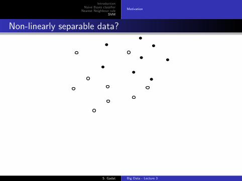
Non-linearly separable data?
S. Gadat Big Data - Lecture 3

IntroductionNaive Bayes classifier
Nearest Neighbour ruleSVM
Motivation
Non-linearly separable data?
S. Gadat Big Data - Lecture 3

IntroductionNaive Bayes classifier
Nearest Neighbour ruleSVM
Motivation
Non-linearly separable data?
S. Gadat Big Data - Lecture 3

IntroductionNaive Bayes classifier
Nearest Neighbour ruleSVM
Motivation
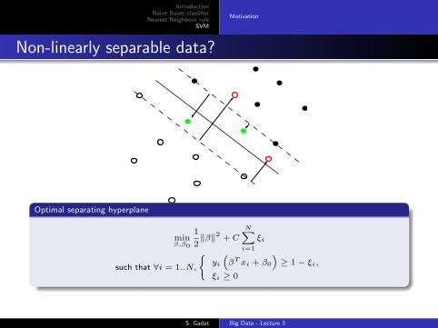
Non-linearly separable data?
Slack variables ξ = (ξ1, . . . , ξN )
yi(βT xi + β0) ≥M − ξi
or
yi(βT xi + β0) ≥M(1− ξi)
and ξi ≥ 0 andN∑i=1
ξi ≤ K
S. Gadat Big Data - Lecture 3

IntroductionNaive Bayes classifier
Nearest Neighbour ruleSVM
Motivation
Non-linearly separable data?
yi(βTxi + β0) ≥M(1− ξi)⇒ misclassification if ξi ≥ 1
N∑i=1
ξi ≤ K ⇒ maximum K misclassifications
S. Gadat Big Data - Lecture 3

IntroductionNaive Bayes classifier
Nearest Neighbour ruleSVM
Motivation
Non-linearly separable data?
Optimal separating hyperplane
minβ,β0‖β‖
such that ∀i = 1..N,
yi(βT xi + β0
)≥ 1− ξi,
ξi ≥ 0,N∑i=1
ξi ≤ K
S. Gadat Big Data - Lecture 3
IntroductionNaive Bayes classifier
Nearest Neighbour ruleSVM
Motivation
Non-linearly separable data?
Optimal separating hyperplane
minβ,β0
1
2‖β‖2 + C
N∑i=1
ξi
such that ∀i = 1..N,
{yi(βT xi + β0
)≥ 1− ξi,
ξi ≥ 0
S. Gadat Big Data - Lecture 3

IntroductionNaive Bayes classifier
Nearest Neighbour ruleSVM
Motivation
Optimal separating hyperplane
Again a QP problem.
LP =1
2‖β‖2 + C
N∑i=1
ξi −N∑i=1
αi(yi(βTxi + β0
)− (1− ξi)
)−
N∑i=1
µiξi
KKT conditions
∂LP∂β = 0⇒ β =
N∑i=1
αiyixi
∂LP∂β0
= 0⇒ 0 =N∑i=1
αiyi
∂LP∂ξ = 0⇒ αi = C − µi
∀i = 1..N, αi(yi(βT xi + β0
)− (1− ξi)
)= 0
∀i = 1..N, µiξi = 0∀i = 1..N, αi ≥ 0, µi ≥ 0
S. Gadat Big Data - Lecture 3

IntroductionNaive Bayes classifier
Nearest Neighbour ruleSVM
Motivation
Optimal separating hyperplane
Dual problem: maxα∈R+N
LD(α) =N∑i=1
αi −1
2
N∑i=1
N∑j=1
αiαjyiyjxTi xj
such thatN∑i=1
αiyi = 0
and 0 ≤ αi ≤ C
S. Gadat Big Data - Lecture 3

IntroductionNaive Bayes classifier
Nearest Neighbour ruleSVM
Motivation
Optimal separating hyperplane
αi(yi(βTxi + β0
)− (1− ξi)
)= 0 and β =
N∑i=1
αiyixi
Again:
αi > 0, then yi(βT xi + β0
)= 1− ξi: xi is a support vector.
Among these:
ξi = 0, then 0 ≤ αi ≤ Cξi > 0, then αi = C (because µi = 0, because µiξi = 0)
αi = 0, then xi does not participate in β.
S. Gadat Big Data - Lecture 3

IntroductionNaive Bayes classifier
Nearest Neighbour ruleSVM
Motivation
Optimal separating hyperplane
Overall:
β =N∑i=1
αiyixi
With αi > 0 only for xi support vectors.
Prediction: f(x) = sign(βT x+ β0
)= sign
(N∑i=1
αiyixTi x+ β0
)S. Gadat Big Data - Lecture 3

IntroductionNaive Bayes classifier
Nearest Neighbour ruleSVM
Motivation
Non-linear SVMs?
Key remark
h :
{X → Hx 7→ h(x)
is a mapping to a p-dimensional Euclidean space.
(p� n, possibly infinite)
SVM classifier in H: f(x′) = sign
(N∑i=1
αiyi〈x′i, x′〉+ β0
).
Suppose K(x, x′) = 〈h(x), h(x′)〉,Then:
f(x) = sign
(N∑i=1
αiyiK(xi, x) + β0
).
S. Gadat Big Data - Lecture 3

IntroductionNaive Bayes classifier
Nearest Neighbour ruleSVM
Motivation
Kernels
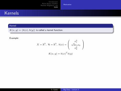
Kernel
K(x, y) = 〈h(x), h(y)〉 is called a kernel function.
S. Gadat Big Data - Lecture 3
IntroductionNaive Bayes classifier
Nearest Neighbour ruleSVM
Motivation
Kernels
Kernel
K(x, y) = 〈h(x), h(y)〉 is called a kernel function.
Example:
X = R2, H = R3
, h(x) =
x21√
2x1x2
x22
K(x, y) = h(x)
Th(y)
S. Gadat Big Data - Lecture 3

IntroductionNaive Bayes classifier
Nearest Neighbour ruleSVM
Motivation
Kernels
Kernel
K(x, y) = 〈h(x), h(y)〉 is called a kernel function.
What if we knew that K(·, ·) is a kernel, without explicitly building h?
The SVM would be a linear classifier in H but we would never have to compute h(x) for trainingor prediction!
This is called the kernel trick.
S. Gadat Big Data - Lecture 3

IntroductionNaive Bayes classifier
Nearest Neighbour ruleSVM
Motivation
Kernels
Kernel
K(x, y) = 〈h(x), h(y)〉 is called a kernel function.
Under what conditions is K(·, ·) an acceptable kernel?Answer: if it is an inner product on a (separable) Hilbert space.
In more general words, we are interested in positive, definite kernel on a Hilbert space:
Positive Definite Kernels
K(·, ·) is a positive definite kernel on X if
∀n ∈ N, x ∈ Xn and c ∈ Rn,n∑
i,j=1
cicjK(xi, xj) ≥ 0
S. Gadat Big Data - Lecture 3

IntroductionNaive Bayes classifier
Nearest Neighbour ruleSVM
Motivation
Kernels
Kernel
K(x, y) = 〈h(x), h(y)〉 is called a kernel function.
Mercer’s condition
Given K(x, y), if:
∀g(x)/
∫g(x)
2dx <∞,
∫∫K(x, y)g(x)g(y)dxdy ≥ 0
Then, there exists a mapping h(·) such that:
K(x, y) = 〈h(x), h(y)〉
S. Gadat Big Data - Lecture 3

IntroductionNaive Bayes classifier
Nearest Neighbour ruleSVM
Motivation
Kernels
Kernel
K(x, y) = 〈h(x), h(y)〉 is called a kernel function.
Examples of kernels:
polynomial K(x, y) = (1 + 〈x, y〉)d
radial basis K(x, y) = e−γ‖x−y‖2
(very often used in Rn)
sigmoid K(x, y) = tanh (κ1〈x, y〉+ κ2)
S. Gadat Big Data - Lecture 3

IntroductionNaive Bayes classifier
Nearest Neighbour ruleSVM
Motivation
Kernels
Kernel
K(x, y) = 〈h(x), h(y)〉 is called a kernel function.
What do you think:Is it good or bad to send all data points in a feature space with p� n?
S. Gadat Big Data - Lecture 3
IntroductionNaive Bayes classifier
Nearest Neighbour ruleSVM
Motivation
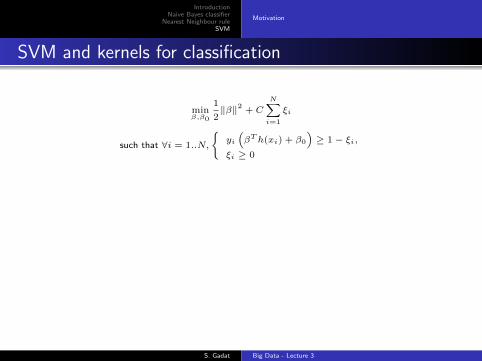
SVM and kernels for classification
minβ,β0
1
2‖β‖2 + C
N∑i=1
ξi
such that ∀i = 1..N,
{yi(βTh(xi) + β0
)≥ 1− ξi,
ξi ≥ 0
S. Gadat Big Data - Lecture 3

IntroductionNaive Bayes classifier
Nearest Neighbour ruleSVM
Motivation
SVM and kernels for classification
minβ,β0
1
2‖β‖2 + C
N∑i=1
ξi
such that ∀i = 1..N,
{yi(βTh(xi) + β0
)≥ 1− ξi,
ξi ≥ 0
Dual problem: maxα∈R+N
LD(α) =
N∑i=1
αi −1
2
N∑i=1
N∑j=1
αiαjyiyj〈h(xi), h(xj)〉
such thatN∑i=1
αiyi = 0
and 0 ≤ αi ≤ C
S. Gadat Big Data - Lecture 3

IntroductionNaive Bayes classifier
Nearest Neighbour ruleSVM
Motivation
SVM and kernels for classification
minβ,β0
1
2‖β‖2 + C
N∑i=1
ξi
such that ∀i = 1..N,
{yi(βTh(xi) + β0
)≥ 1− ξi,
ξi ≥ 0
Dual problem: maxα∈R+N
LD(α) =
N∑i=1
αi −1
2
N∑i=1
N∑j=1
αiαjyiyjK(xi, xj)
such thatN∑i=1
αiyi = 0
and 0 ≤ αi ≤ C
S. Gadat Big Data - Lecture 3

IntroductionNaive Bayes classifier
Nearest Neighbour ruleSVM
Motivation
SVM and kernels for classification
Overall:β =
N∑i=1
αiyixi
With αi > 0 only for xi support vectors.
Prediction: f(x) = sign(βT x+ β0
)= sign
(N∑i=1
αiyiK(xi, x) + β0
)
S. Gadat Big Data - Lecture 3

IntroductionNaive Bayes classifier
Nearest Neighbour ruleSVM
Motivation
Why whould you use SVM?
With kernels, sends the data into higher (sometimes infinite) dimension feature space, wherethe data is separable / linearly interpolable.
Produces a sparse predictor (many coefficients are zero).
Automatically maximizes margin (thus generalization error?).
Performs very well on complex, non-linearly separable / fittable data.
S. Gadat Big Data - Lecture 3

IntroductionNaive Bayes classifier
Nearest Neighbour ruleSVM
Motivation
SVM for regression
Now we don’t want to separate, but to fit.
Contradictory goals?
Fit the data: minimizeN∑i=1
V (yi − f(xi))
V is a loss function.
Keep large margins: minimize ‖β‖
Support Vector Regression
minβ,β0
1
2‖β‖2 + C
N∑i=1
V (yi − βT xi + β0))
S. Gadat Big Data - Lecture 3

IntroductionNaive Bayes classifier
Nearest Neighbour ruleSVM
Motivation
Loss functions
ε-insensitive V (z) =
{0 if |z| ≤ ε|z| − ε otherwise
Laplacian V (z) = |z|Gaussian V (z) = 1
2 z2
Huber’s robust loss V (z) =
{1
2σ z2 if |z| ≤ σ
|z| − σ2 otherwise
S. Gadat Big Data - Lecture 3
IntroductionNaive Bayes classifier
Nearest Neighbour ruleSVM
Motivation
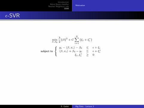
ε-SVR
minβ,β0
λ
2‖β‖2 + C
N∑i=1
(ξi + ξ
∗i
)
subject to
yi − 〈β, xi〉 − β0 ≤ ε+ ξi〈β, xi〉+ β0 − yi ≤ ε+ ξ∗i
ξi, ξ∗i ≥ 0
As previously, this is a QP problem.
LP =λ
2‖β‖2 + C
N∑i=1
(ξi + ξ
∗i
)−
N∑i=1
αi (ε+ ξi − yi + 〈β, xi〉+ β0)
−N∑i=1
α∗i
(ε+ ξ
∗i + yi − 〈β, xi〉 − β0
)−
N∑i=1
(ηiξi + η
∗i ξ∗i
)
S. Gadat Big Data - Lecture 3

IntroductionNaive Bayes classifier
Nearest Neighbour ruleSVM
Motivation
ε-SVR cont’d
LD = −1
2
N∑i=1
N∑j=1
(αi − α∗i
) (αj − α∗j
)〈xi, xj〉
− εN∑i=1
(αi + α
∗i
)+
N∑i=1
yi(αi − α∗i
)Dual optimization problem:
maxα
LD
subject to
N∑i=1
(αi − α∗i ) = 0
αi, α∗i ∈ [0, C]
S. Gadat Big Data - Lecture 3

IntroductionNaive Bayes classifier
Nearest Neighbour ruleSVM
Motivation
ε-SVR, support vectors
KKT conditions:
αi (ε+ ξi − yi + 〈β, xi〉+ β0) = 0
α∗i (ε+ ξ∗i − yi + 〈β, xi〉+ β0) = 0
(C − αi) ξi = 0
(C − α∗i ) ξ∗i = 0
if α(∗)i = 0, then ξ
(∗)i = 0: points inside the ε-insensitivity “tube” don’t participate in β
if α(∗)i > 0, then
if ξ(∗)i = 0, then xi is exactly on the border of the “tube”,
α(∗)i ∈ [0, C]
if ξ(∗)i > 0, then α
(∗)i = C: outliers are support vectors.
S. Gadat Big Data - Lecture 3

IntroductionNaive Bayes classifier
Nearest Neighbour ruleSVM
Motivation
SVR prediction
f(x) =N∑i=1
(αi − α∗i
)〈xi, x〉+ β0
S. Gadat Big Data - Lecture 3

IntroductionNaive Bayes classifier
Nearest Neighbour ruleSVM
Motivation
Kernels and SVR?
Just as you would expect it!Left to you as an exercice.
S. Gadat Big Data - Lecture 3

IntroductionNaive Bayes classifier
Nearest Neighbour ruleSVM
Motivation
Why whould you use SVM?
With kernels, sends the data into higher (sometimes infinite) dimension feature space, wherethe data is separable / linearly interpolable.
Produces a sparse predictor (many coefficients are zero).
Automatically maximizes margin (thus generalization error?).
Performs very well on complex, non-linearly separable / fittable data.
S. Gadat Big Data - Lecture 3

IntroductionNaive Bayes classifier
Nearest Neighbour ruleSVM
Motivation
Further reading / tutorials
A tutorial on Support Vector Machines for Pattern Recognition.C. J. C. Burges, Data Mining and Knowledge Discovery, 2, 131–167, (1998).
A tutorial on Support Vector Regression.A. J. Smola and B. Scholkopf, Journal of Statistics and Computing, 14(3), 199-222, (2004).
S. Gadat Big Data - Lecture 3