bim model data transfer from revit into static analysis
TRANSCRIPT

Author: Zhu Nan, B.Sc. ZURICH | 2019
BIM model data transfer from Revit into static analysis software: development of a plug-in based on Revit
MASTER THESIS SPRING SEMESTER 2019 ETH ZURICH
START FROM: 18.02.2019
SUBMITTED ON: 01.07.2019
INSTITUTE: INSTITUTE FOR GEOTECHNICAL ENGINEERING, ETH ZURICH
INSTITUTE FOR CONSTRUCTION INFORMATICS, TU DRESDEN
AMBERG ENGINEERING AG, AMBERG GROUP
SUPERVISORS: PROF. DR. I. ANASTASOPOULOS, ETH ZURICH
PROF. DR. R. J. SCHERER, TU DRESDEN
DR. A. MARIN, ETH ZURICH
MSC. F. LIN, TU DRESDEN
MSC. L. SAKELLARIADIS, TU DRESDEN
AMBERG GROUP: MSC. P. DOHMEN
MSC. A. TATAR

Masterarbeit 2019
1
Preface The idea of this master thesis originally comes from Mr. Ali Tatar during my intern from September
2018 to January 2019 in Amberg Engineering AG in Zurich. He was the leader of BIM department of
Amberg Engineering AG at that time and has found the necessity of extracting and transferring model
parameter from BIM software into static analysis software. This technic provides the possibility to
considerably shorten the working time for both BIM drafters and civil engineers. After the dimission
of Mr. Tatar, Mr. Philipp Dohmen, leader of digitization of Amberg Group Ltd, has taken over this
master thesis and supervised me during the whole period of the thesis. I must express my heartfelt
thanks for Mr. Tatar and Mr. Dohmen for the help from them in every possible way. I must also thank
Mr. Abdelali Aouada, BIM computational specialist in Amberg Engineering AG, for offering me Revit
models.
For the guidance of data extraction and transfer of BIM model, I must thank Prof. R. J. Scherer and
Mr. Fangzheng Lin (Institute for Construction Informatics, TU Dresden). They have given me support
and guidance not only in the field of model data extraction from BIM software, but also the CADINP
language of static analysis software SOFiSTiK. Mr. Lin has given me overwhelming support during the
whole period of my master thesis, to prevent me from deviating from the right path.
For the aspect of static analysis of the extracted BIM model, I would like to firstly thank my thesis
advisor Prof. Dr. I. Anastasopoulos (Institute for Geotechnical Engineering, ETH Zurich), who is quite
open for my master thesis and has steered me in the right direction whenever he thought I need it. I
would also like to thank Dr. A. Marin (Institute for Geotechnical Engineering, ETH Zurich), my main
supervisor during the whole period of my thesis, for keeping giving me valuable comments and help.
Without his passionate contribution, the master thesis cannot be successfully finished. I would also
like to thank MSc. L. Sakellariadis for helping me simulating the pile-soil interface and pointing out
the problems of my hand calculation in time.
Finally, I must express my profound gratitude to my parents for providing me with unfailing support
and continuous encouragement. Without their support, the accomplishment of my master study
cannot be possible. Thank you!
Nan Zhu

Masterarbeit 2019
2
Kurzfassung Eines der Hauptmerkmale der Building Information Modeling (BIM) ist die zentrale
Datenspeicherung. Diese Modelldaten (z. B. Abmessungen, Koordinaten, Materialien usw.) können in
der BIM-Software Revit mithilfe der Revit-API-Funktionen extrahiert werden. Mit den extrahierten
Modelldaten werden mithilfe von Abaqus-Makrofunktionen neue Modelle für die statische Analyse
in den statischen Analysesoftware Abaqus und SOFiSTiK erstellt. Die Erstellung und Vernetzung des
statischen Modells erfolgt in Abaqus mithilfe von Python-gesteuerten Abaqus-Makrofunktionen. Die
vernetzten Modelldaten werden dann in Form einer Abaqus-Eingabedatei und einer SOFiSTiK-
Eingabedatei (CADINP-Sprache) zur weiteren statischen Analyse geschrieben.
In dieser Masterarbeit wurden Pfahlgruppenfundament und Tunnelmodell getestet, um die
Anwendbarkeit und Robustheit der BIM-Datenübertragung zu überprüfen. Die Gründung der
Pfahlgruppe wurde speziell für die detaillierte statische Analyse in Abaqus ausgewählt.
Die manuelle Vorverarbeitung von Pfahlgruppenfundamenten ist zeitaufwändig und fehleranfällig.
Somit wird ein standardisierter Vorverarbeitungsworkflow des FEM-Modells unter Verwendung eines
pythongesteuerten Abaqus-Makros implementiert. Die korrekte Vorverarbeitung wird zunächst bei
gleichzeitiger Abaqus-Makroaufnahme durchgeführt. Anschließend werden die nützlichen
Informationen im Abaqus-Makroskript extrahiert, um ein verständliches Python-Skript neu zu
erstellen. Mit dem Python-Skript wird Abaqus CAE so gesteuert, dass eine System-Eingabedatei
generiert wird, die mit vielen nutzlosen Informationen nicht sauber und verständlich genug ist. Auf
diese Weise wird anschließend eine neue saubere und verständliche Eingabedatei erstellt, indem
Python-Skripte für weitere statische Analysen verwendet werden.
Nach der erfolgreichen Erstellung des Abaqus-Plugins zur automatischen Generierung des
Pfahlgruppengrundmodells wird die laterale Pushover-Analyse der Pfahlgruppe durchgeführt. Die
Momentenkapazität einer Pfahlgruppe wird herkömmlicherweise als das Moment definiert, das
mobilisiert wird, wenn die Randpfähle einer Gruppe ihre axiale bzw. Druckkapazität erreichen. So
werden zunächst die vertikalen Druck- und Zugprüfungen für Einzelpfähle zur Entnahme von Druck-
und Zugkräften durchgeführt. Danach werden Biegemomente, die durch Rotation des Fundaments in
den Pfählen induziert werden, ebenfalls als wichtiger Faktor der Momentenkapazität für die
Pfahlgruppe angesehen. In diesem Fall ist die Momentenkapazität für Pfahlgruppen durch die
Biegekapazität der Pfähle begrenzt. Daher wird eine Untersuchung der
Pfahlgruppenmomentwiderstand unter Berücksichtigung nicht nur der herkömmlichen Druck- und
Zugwiderstand, sondern auch der Biegemomentwiderstand der Pfählen durchgeführt, um den
Entwurfsprozess zu optimieren und unnötigen Konservativismus zu reduzieren.

Masterarbeit 2019
3
Abstract One of the main characteristics of building information modelling (BIM) is the central data storage.
These model data (e.g. dimensions, coordinates, materials, etc.) can be extracted in BIM software
Revit by using Revit API functions. With the extracted model data, new models for static analysis are
created in static analysis software Abaqus and SOFiSTiK, by using Abaqus macro functions. The
creation and mesh of static model are conducted in Abaqus by using python controlled Abaqus
macro functions. The meshed model data are then written in the form of Abaqus input file and
SOFiSTiK input file (CADINP language), for further static analysis.
This thesis has tested pile group foundation and tunnel model, to check the applicability and
robustness of BIM data transfer. Pile group foundation is specifically selected for detailed static
analysis in Abaqus.
Manual pre-processing of pile group foundation is time-consuming and error prone. Thus, a
standardized pre-processing workflow of FEM model is implemented, using python controlled
Abaqus macro. The correct pre-processing is conducted at first, with Abaqus macro recording at the
same time. Then, the useful information in Abaqus macro script is extracted for regeneration of an
understandable python script. Using the python script, Abaqus CAE is controlled to generate a
system input file, which is not clean and understandable enough with many useless information.
Thus, a new clean and understandable input file is created afterwards by using python script for
further static analysis.
After the successful creation of Abaqus plugin, for automatic generation of pile group foundation
model, the lateral pushover analysis of pile group is conducted. Moment capacity of a pile group is
conventionally defined as the moment mobilized when the edge piles of a group reach their axial and
compressive capacity respectively. Thus, the vertical compression and tension tests for single pile are
firstly conducted for extraction of compressive and tensive capacities. After that, bending moments
induced in the piles due to rotation of the foundation are also considered as an important factor of
moment capacity for pile group. In this case, the moment capacity for pile group is limited by the
bending capacity of the piles. Thus, investigation of pile group moment capacity considering not only
conventional compression and tension capacity, but also bending moment capacity of piles, is
conducted for optimization of the design process and the reduction of unnecessary conservatism.

Masterarbeit 2019
4
Contents Preface ..................................................................................................................................................... 1
Kurzfassung ............................................................................................................................................. 2
Abstract ................................................................................................................................................... 3
1. Introduction ......................................................................................................................................... 6
1.1. Introduction and status quo ......................................................................................................... 6
1.2. Goals of the work ......................................................................................................................... 8
1.3. Structure of the master thesis ...................................................................................................... 9
2. Literature review ............................................................................................................................... 11
3. Drafting in Revit ................................................................................................................................. 12
4. Data transfer from Revit to Abaqus .................................................................................................. 14
4.1. Extraction of model data in Revit ............................................................................................... 14
4.2. Adjustment of coordinate systems from Revit to Abaqus ......................................................... 16
4.3. Generation of Abaqus input file with extracted data from Revit model ................................... 16
4.4. Transfer demonstration from Revit into Abaqus ....................................................................... 18
5. Modelling in Abaqus .......................................................................................................................... 20
5.1. Modeling of pile.......................................................................................................................... 20
5.1.1. Moment curvature (MC) pile ............................................................................................... 20
5.1.2. Concrete damaged plasticity (CDP) pile .............................................................................. 21
5.2. Modeling of soil .......................................................................................................................... 22
5.3. Modeling of pile cap and pier ..................................................................................................... 23
5.4. Interface between pile and soil .................................................................................................. 24
5.5. Connections management ......................................................................................................... 25
5.5.1. Connections on pier ............................................................................................................ 25
5.5.2. Connections between pier and pile cap .............................................................................. 25
5.5.3. Connections between MC pile and pile cap ........................................................................ 26
5.5.4. Connections between CDP pile and pile cap ....................................................................... 26
5.5.5. Connections between pile cap and soil ............................................................................... 26
6. Automatic modelling in Abaqus ........................................................................................................ 27
6.1. Brief introduction to Abaqus macro ........................................................................................... 27
6.2. User interface for parameter input ............................................................................................ 27
6.3. Automatic modelling procedure ................................................................................................ 28
7. Push-over analyses (results and interpretation) ............................................................................... 30
7.1. Vertical compression test for single pile .................................................................................... 30
7.1.1. Hand calculation results for compression pile .................................................................... 30
7.1.2. Numerical modelling results for compression pile .............................................................. 31

Masterarbeit 2019
5
7.1.3. Comparison between results from hand calculation and numerical modelling ................. 32
7.2. Vertical tension test for single pile ............................................................................................. 34
7.2.1. Hand calculation results for tension pile ............................................................................. 34
7.2.2. Numerical modelling results for tension pile ...................................................................... 34
7.2.3. Comparison between results from hand calculation and numerical modelling ................. 35
7.3. Lateral pushover analysis for pile group foundation.................................................................. 35
7.3.1. Analytical method for rotation of pile group foundation according to GAZETAS (1991) ... 36
7.3.2. Numerical modelling results for pile group ......................................................................... 36
8. Discussion .......................................................................................................................................... 39
9. Outlook .............................................................................................................................................. 40
Appendices ............................................................................................................................................ 41
Appendix A ........................................................................................................................................ 42
A1. Hand calculation of vertical capacity for single pile ................................................................ 42
A2. Hand calculation for pile group ............................................................................................... 47
Appendix B ........................................................................................................................................ 49
B1: Design structure and workflow of python script .................................................................... 49
B2: Python codes ........................................................................................................................... 81
Figure lists .............................................................................................................................................. 82
Table lists ............................................................................................................................................... 85
List of abbreviations .............................................................................................................................. 86
References ............................................................................................................................................. 87

Masterarbeit 2019
6
1. Introduction
1.1. Introduction and status quo Building Information Modelling (BIM), a 3D based modelling method with model information
combined, should lead to more transparency, better planning and deadline and cost certainty in
construction. One of the main characteristics of building information modelling (BIM) is the central
data storage, which can be used for different purposes (e.g. construction guidance, cost estimation,
static analysis, etc.).
As a leading company in the field of BIM and civil engineering industry in Switzerland, Amberg
Engineering AG has found the necessity of creating the interface of BIM software, for BIM model
data extraction and implementation for practical engineering application. This master thesis is
written during the author’s intern in BIM department of Amberg Engineering AG.
To improve the communication efficiency between architects and civil engineers, a Revit plug-in is
developed for reading and extracting BIM model data. These model data (e.g. dimensions,
coordinates, materials, etc.) can be extracted in BIM software Revit by using Revit API functions. With
the extracted model data, new models for static analysis are created in static analysis software
Abaqus and SOFiSTiK, by using Abaqus macro functions.
Two static analysis software, Abaqus and SOFiSTiK are specifically selected. Abaqus is a powerful FEM
software with abundant linear and non-linear analysis tools. Moreover, it also contains an ample
macro functions library, which can conduct the pre-processing of FEM model automatically by using
python controlled Abaqus macro functions. The meshed model data are then written in the form of
Abaqus input file and SOFiSTiK input file (CADINP language), for further static analysis. SOFiSTiK,
another powerful static analysis software in civil engineering industry, is not able to simulate the
whole FEM model by script automatically. The generation and mesh of a FEM model can only be
conducted in its integrated software SOFiPlUS manually. Thus, Abaqus is purposely selected, for
preparation of meshed nodes and elements in SOFiSTiK.
After the preparation of BIM model and data transfer, static analysis should be conducted.
This thesis has tested pile group foundation and tunnel model, to check the applicability and
robustness of BIM data transfer. Pile group foundation is specifically selected for detailed static
analysis in Abaqus, whereas the static analysis of tunnel model will not be considered in this thesis.
For bridge engineering, the most commonly used foundation type is pile, with different types of cross
sections. Among all these types of piles, circular pile is frequently used for shallow foundations and
has a relatively clear static mechanism. When the bearing capacity of surface soil layers is
insufficient, the loads on the foundation need to be transferred to deeper soil layers via piles.
Besides the bearing resistance for foundation, pile foundations can also be adopted when
settlements need to be reduced or when the available space for the foundation system is limited.
This thesis focuses on circular pile foundation, based on conventional theory of pile capacity. The
transfer of vertical loads from superstructure to the ground happens via the shear stresses mobilized
along the shaft at the contact between pile and surrounding soil, and normal stresses at the pile tip.
This means the pile bearing system consists of three cases:
Case 1: the pile can be floating, which means shaft friction along the pile is significantly higher than
tip pressure.
Case 2: the pile can be end bearing. In this regard, the loads are mostly transferred by means of
pressure mobilized at the pile tip.

Masterarbeit 2019
7
Case 3: the pile can be hybrid bearing, which indicates the both the shaft friction and the tip pressure
have non-negligible contribution to the bearing capacity
This thesis has assumed that pile tip has not reached the rock. An isotropic undrained soil layer with
a relatively common shear strength (100 kPa) is selected for analysis. Thus, case 3 is more suitable for
simulation of axial compression mechanism.
For simulation of this kind of mechanism, there are a lot of commercial and educational finite
element software. For this thesis, Abaqus CAE is selected for pre-processing and finite element
modeling. This is a powerful finite element analysis software, which contains all types of finite
element with linear and non-linear analysis tools. Moreover, Abaqus owns a powerful python-based
macro, which can record all manual steps during modelling. This enables the further standardized
automatic modelling process in chapter 6.
In order to properly simulate the axial and lateral pushover mechanism of pile, not only all elements
in the whole pile should be driven axially and move at the same pace, as it has a relatively larger
elastic modulus and stiffness than soil, but the materials’ constitutive laws should also be correctly
defined.
The pile is firstly simulated as a centralized located beam which controls the surrounding pseudo
solid elements. The advantage of this simulation method is that the definition of the beam properties
is relatively easier (only need to define the beam elements) than to simulate the whole pile structure
with solid elements. Moreover, the beam element can properly simulate the axial movement and
even lateral bending procedure of a real pile. Thus, this kind of modelling method is marked as
moment curvature (MC) pile in this thesis. However, one challenge to precisely simulate the pile
structure is that the moment curvature relationship is always not constant during lateral pushover
progress. Th axial load on the pile varies during the lateral pushover progress, which leads to variant
moment curvature relationships of pile. It is a big challenge to accurately put the adjusted moment
curvature data (corresponds to adjusted axial load) into Abaqus input file every time the axial load
changes during the lateral pushover progress.
Thus, it is inevitable to model the whole pile with solid elements and define the individual properties
of them. This method can indeed precisely simulate the real pile properties during lateral pushover
progress. However, the modelling progress (CDP) is relatively more complex than the former method
(MC). As the pile element consists of three parts: internal confined concrete, reinforcement in the
middle and unconfined concrete outside. This pile is the so-called concrete damaged plasticity (CDP)
pile, with predefined damage and stress development curves along with increasing inelastic strain.
The later modelling method (CDP pile) is a standard comparison against the former method (MC pile)
It is quite time consuming and error prone to simulate the MC and CDP pile foundations mentioned
above in Abaqus. The engineers and researchers cannot focus on the most meaningful static analysis
part at the beginning of the simulation. Thus, a standardized and automatic modelling tool for these
two types of pile group foundations is necessary and meaningful. With this tool, the engineers can
firstly focus on the design and static analysis part as follows.
For design and static analysis of pile group foundation, especially for overturning moment on pile
group, the moment capacity of pile group is mobilized mainly by two mechanisms. One mechanism
of moment capacity is due to the contribution of compression and tension axial forces induced in the
pile according to their distance to the center of rotation of the foundation. In this regard, the
moment capacity of the whole pile group is limited by the axial compression and tension resistance
of the edge piles. This mechanism is the main contribution to the pile group’s overturning moment
capacity. Another mechanism stays in the bending moments induced in the piles due to the rotation

Masterarbeit 2019
8
of the pile group foundation. In this case, the pile group overturning capacity is strictly limited by the
bending moment capacity of single pile, which have relatively less contribution to the whole
overturning moment capacity of pile group. The conventional design for pile group considers only the
first mechanism and contains unnecessary conservatism. Thus, besides the automation of finite
element modelling procedure for pile group, the study of the second mechanism of moment capacity
for pile group is also necessary, to avoid unnecessary conservatism.
1.2. Goals of the work As is already introduced above, one main goal of the thesis is to build a powerful tool (in the form of
plug-ins) both in BIM software Revit and static analysis software Abaqus. The whole workflow of this
master thesis is shown in Figure 1. At first, the accurate data extraction of parametric model in BIM
software should be conducted, by using C# script and Revit API functions, for further pre-processing
of FEM model. Then, a standardized constitutive and numerical modelling process should be built,
based on the parameters extracted from the first step. After the determination of numerical
modelling method, the input language of FEM software Abaqus and SOFiSTiK should be studied and
used for generation of input file. With the preparation work above, an automatic modelling
procedure should be realized by using python script. An Abaqus plug-in should be built in this step to
realize these functions. Finally, the static analysis will be conducted. In this thesis, two types of pile
group foundations, moment curvature and concrete damaged plasticity pile, are selected for static
analysis.
Figure 1: Workflow of this master thesis
In order to automatically simulate the moment curvature and concrete damaged plasticity pile
foundations in Abaqus, a proper and standardized simulation progress of these two pile group
foundations will be introduced at first. Then, following the standardized simulation progress, a plugin
for Abaqus will be created by using python script and Abaqus macro. This part of work is like the
assembly line of Henry Ford’s model T car assembly line (Figure 2), which has significantly increased
the work efficiency of car industry. The engineers can create their finite element model by simply

Masterarbeit 2019
9
giving the essential parameters in the Abaqus plugin or drafting in BIM software Revit, and then the
whole model will be generated automatically in the form of a ready-to-run input file in a few
seconds.
Figure 2: Henry Ford’s model T car assembly line
After the creation of Abaqus plugin for automatic model generation, static analysis for overturning
moment capacity of pile group should be conducted. As is already explained in section 1.2, the
second mechanism (bending moment of single pile) which contributes to the overturning moment
capacity of the whole pile group should also be considered.
Figure 3 shows the three stages of overturning moment added on pile group. Point A indicates the
stage where the edge piles of the pile group reach their compression resistance, while the tension
piles on the other side haven’t reached their tension resistance. The curve from point A to point B
represents the progress that the compression edge piles stay at the limit state, while the tension
edge piles slowly come to the tension resistance. The interval from point B to point C implies that
edge piles on both sides have reached their tension and compression resistance, but the piles haven’t
reached their bending moment resistance yet. Point C is the time when one of the piles in the pile
group firstly reaches its bending moment resistance. This means the whole pile group comes to
failure.
Figure 3: three overturning moment stages for pile group foundation
The task is to conduct the numerical analysis of pile group and extract the moment curvature data to
find these three points on the curve.
1.3. Structure of the master thesis At the beginning, literature review is performed in chapter 2 to summarize the evaluation methods
of bearing capacity of piles.
After the illustration of pile foundation typologies and bearing capacity in chapter 2, the geometry pf
the foundation will be drafted using Revit (BIM software Autodesk). Introduction to Revit will be
conducted at first. Then the drafting method will also be briefly introduced in chapter 3. This part of

Masterarbeit 2019
10
work is preparation for work in chapter 4: data transfer from Revit into Abaqus. In chapter 4, Revit
API (application programming interface) will be introduced at first, to show the data extraction from
parametric model in Revit. Then an Abaqus plugin, which can read the extracted pile dimensions
from Revit, will be introduced.
To realize the automatic modelling procedure, a standardized manual modelling is firstly conducted
in chapter 5. Then chapter 6 and appendix A will introduce the automatic modelling procedure with
python script.
With the pre-processed model above, pushover analysis is carried out in chapter 7 and the results
will be analysis and interpreted in this chapter.
Chapter 8 summarizes the whole thesis and gives a review of all the work and results in this thesis.
The possible studies in the future based on this thesis will be discussed in chapter 9.
Besides the main structure of this thesis, two appendices are appended in the end. Appendix A gives
all the details of hand calculation about bear capacity for pile and pile group foundations. Then
appendix B shows the whole development procedure of Abaqus plugin, which is specially designed
for automatic modelling of pile group foundations.

Masterarbeit 2019
11
2. Literature review As is already introduced in chapter 1, a standard pile foundation modelling workflow should be
conducted in this thesis. To test the validity of the model, analytical methods of pile bearing capacity
should be selected. For pile bearing capacity for undrained conditions, analytical methods from both
Lang et al. (2011) and EA Pfähle are selected as comparison to numerical results.
For analytical method of Lang et al. (2011), the shaft resistance of pile only depends on the pile
dimension and undrained shear strength between pile and soil. The undrained shear strength on the
shaft is acquired by adding a reduction factor to the undrained shear strength of soil. In this thesis, a
reduction factor of 0.7 is selected. For base resistance, the method from Lang et al. (2011) considers
the effect of slenderness ratio of pile, the cross-section area of pile and the undrained shear strength
of soil. The analytical method from Lang et al. (2011) has simplified the calculation progress and
makes the mechanism clear and understandable. However, the influence of the settlement of pile on
pile base resistance has not be considered.
Empirical method (EA Pfähle) has eliminated the drawback. The pile shaft resistance is firstly
acquired with a range of empirical values according to the undrained shear strength of soil. Then the
settlement of the pile is divided into three stages, where the settlement reaches 0.02D, 0.03D and
0.1D (D=diameter of pile) respectively. Different from the method of Lang et al. (2011), base
resistance of pile according to EA Pfähle is not constant anymore. It depends on the undrained shear
strength of soil and relative settlement of the pile. Base resistance increases with increasing
settlement until the settlement reaches 0.1D.
After determining the bearing capacity for single pile, analytical method for the rotation of pile group
foundation should also be selected, as comparison to the results from numerical model. GAZETAS
(1991) has divided the rotational stiffness of pile group into two parts. The axial stiffness of edge
piles on both sides of pile group and the rotational stiffness of pile itself. The axial stiffness of single
pile was developed by Randolph & Wroth (1978), by considering the pile-soil stiffness ratio and
influence radius of pile. The self-rotational stiffness of pile also depends on pile-soil stiffness ratio
and elastic modulus of soil. The analytical rotational stiffness is then acquired for comparison to the
results from numerical pushover analysis.
Besides the definition of pile properties, the soil also plays an important role during pushover
analysis. For failure criteria of soil, the modified von-mises failure criteria is selected, instead of
Mohr-Coulomb failure criteria, to simulate the soil failure behavior. Although Mohr-Coulomb failure
criteria provides a good fit to the experimental data in triaxial compression and extension, it is not
the most convenient model to use, either for analytical or numerical analysis (Puzrin (2012)).
For analytical analysis with Mohr-Coulomb failure criteria, the analytical derivations, based on the
complex expression of failure surface in the stress tensor invariant space, are extremely complicated.
For numerical case, the numerical analysis may easily run into difficulties, as the surface in 3D
principal stress space is not “smooth”, it has “corners”.
Those difficulties are eliminated by modified Von-Mises failure criteria. The surface of Von-Mises
failure criteria in 3D principal stress space is a cylinder. To let the failure surface fit the Mohr-
Coulomb failure surface, a modified Von-Mises cone surface was applied by Anastasopoulos (2011).
Masterarbeit 2019
12
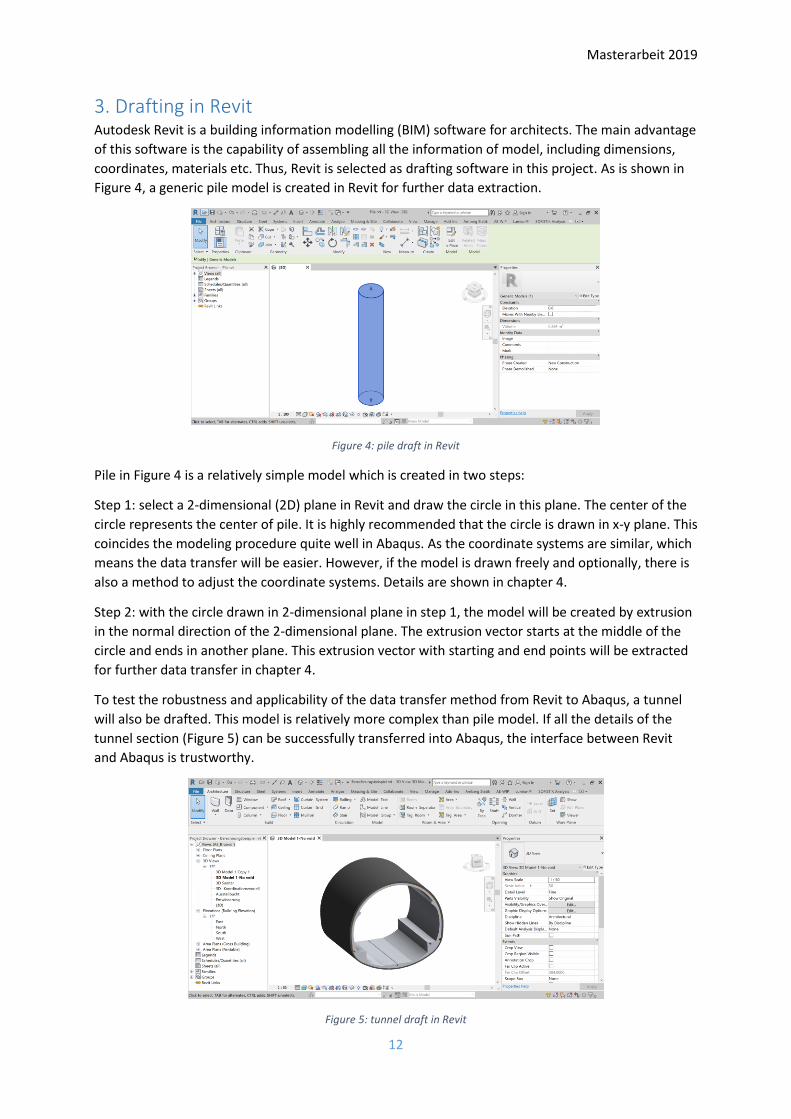
3. Drafting in Revit Autodesk Revit is a building information modelling (BIM) software for architects. The main advantage
of this software is the capability of assembling all the information of model, including dimensions,
coordinates, materials etc. Thus, Revit is selected as drafting software in this project. As is shown in
Figure 4, a generic pile model is created in Revit for further data extraction.
Figure 4: pile draft in Revit
Pile in Figure 4 is a relatively simple model which is created in two steps:
Step 1: select a 2-dimensional (2D) plane in Revit and draw the circle in this plane. The center of the
circle represents the center of pile. It is highly recommended that the circle is drawn in x-y plane. This
coincides the modeling procedure quite well in Abaqus. As the coordinate systems are similar, which
means the data transfer will be easier. However, if the model is drawn freely and optionally, there is
also a method to adjust the coordinate systems. Details are shown in chapter 4.
Step 2: with the circle drawn in 2-dimensional plane in step 1, the model will be created by extrusion
in the normal direction of the 2-dimensional plane. The extrusion vector starts at the middle of the
circle and ends in another plane. This extrusion vector with starting and end points will be extracted
for further data transfer in chapter 4.
To test the robustness and applicability of the data transfer method from Revit to Abaqus, a tunnel
will also be drafted. This model is relatively more complex than pile model. If all the details of the
tunnel section (Figure 5) can be successfully transferred into Abaqus, the interface between Revit
and Abaqus is trustworthy.
Figure 5: tunnel draft in Revit

Masterarbeit 2019
13
The way to draft the tunnel section is the same as that for pile. A 2-dimensional plane should be
firstly selected for drawing faces to extrude. This tunnel section consists of four parts, namely shot-
concrete calotte, sealing, tunnel inner lining and in-situ concrete shoulder. All these parts are
extruded sections. Thus, the first step is to draw all the faces of them with lines and curves in a plane.
After finishing the closed faces, the model can be created by extrusion afterwards.
Until now, a simple pile model and a relatively more complex tunnel model are prepared.

Masterarbeit 2019
14
4. Data transfer from Revit to Abaqus
4.1. Extraction of model data in Revit In order to extract coordinates of Revit model, the Revit application programming interface (API) is
employed. Autodesk Revit API platform holds a very rich function library, compatible with
Microsoft .NET framework such as C# and VB. By accessing the API functions, the model information
such as coordinates can be extracted for further use.
Autodesk Revit API development library contains a lot of namespaces as shown in Figure 6.
Namespace “Autodesk.Revit.DB” includes all the information of Revit functions and Revit model. The
coordinates and dimensions of Revit model should be extracted from this namespace. Besides
“Autodesk.Revit.DB”, namespace “Autodesk.Revit.UI” deals with functions about user interface.
Functions in these two namespaces will be visited and accessed for extraction of model information.
Figure 6: namespaces of Revit API development platform

Masterarbeit 2019
15
Figure 7: Revit API function to extract extrusion vector
Figure 7 shows the method to acquire extrusion vector of model. As is already shown in chapter 3,
the model is created with extruded faces. Thus, the vector for face extrusion should be extracted
from Revit at first. Under the namespace “Autodesk.Revit.DB” in class
“AdaptiveComponentInstanceUtils”, method “GetInstancePlacementPointElementRefIds” can extract
the extrusion vector’s starting and end points’ coordinates. Details of the codes are appended in the
handed file “Revit_Finalreader”. It should be mentioned that all the codes are written with object-
oriented programming language C#.
Figure 8: Revit API function to find faces for extrusion
After successful extraction of extrusion vector’s coordinates, the faces for extrusion should also be
found and selected. In namespace “Autodesk.Revit.DB” there is a class called solid, which represents
all solid elements in Revit. By accessing its properties edges and faces, all the faces and edges of a
solid element can be selected for further use.
For recognition of extruded faces, cross validation is used. The normal of selected face and extrusion
vector will cross validate (Figure 8). If the value of cross validation is nearly negligible, this means the
normal of the face is parallel to the extrusion vector. This means the face is the right face for
extrusion.
With the extruded face, class “Face” will be used (Figure 9) to access the edges of the face. This
property of class “Face” will export lines and curves of face edges in sequence. The coordinates of all
edges can be extracted by using this method.

Masterarbeit 2019
16
Figure 9: Revit API function to extract coordinates of edge lines and curves
With methods above, curves and lines in face edges, in form of coordinates of starting points, end
points and middle points, can be written in the form that Abaqus can recognize. The basic steps to
create model are the same as that in Revit (shown in chapter 3). Thus, same model can be generated
again in Abaqus with the parameters extracted above.
4.2. Adjustment of coordinate systems from Revit to Abaqus One challenge during data transfer from Revit to Abaqus stays in the coordinate system. As is already
shown in chapter 3, the model is created firstly with face in a 2-dimensional plane before extrusion.
This plane can be x-y, y-z or x-z plane. However, the model might be rotated afterwards, which
indicates that the coordinates of faces is no longer in x-y, y-z or x-z plane anymore.
Thus, the model must be rotated back with faces in standardized plane at first. Then the extrusion
vector can be extracted for further modelling.
4.3. Generation of Abaqus input file with extracted data from Revit model To generate Abaqus input file with the extracted coordinates above, Abaqus macro should be used.
The common way to create the model in Abaqus is using the Abaqus user interface directly. The finite
element model is created step by step manually, according to the dimensions of model extracted
above. After finishing the modeling work, a system input file can be generated for calculation. All the
steps above can be recorded by Abaqus macro, including the generation of system input file. Thus,
data transfer from Revit to Abaqus can be realized automatically by two steps: exporting data from
Revit at first and then importing data in Abaqus.
For step one, exporting data from Revit, a Revit plugin (Figure 10) using Revit API (application
programming interface) functions is created, for reading model dimensions and coordinates at first,
and then exporting the data into a json file. It can be seen in Figure 10 that the plugin is called
“Amberg Statik”. “Amberg” is an engineering company in Switzerland where the author works in. The
goal of this plugin later is to develop a powerful interface which can export all types of elements (e.g.
beams, columns etc.) into json file for further use. In this thesis, only the interface about pile and
tunnel will be introduced.
Figure 11 demonstrates the structure of this Revit plugin, which can export the data into two types of
files: dat file for commercial FEM software SOFiSTiK and json file for Abaqus. This thesis only deals
with the part about Abaqus. It can be clearly seen in Figure 11 that the user can input dimensions of
soil surrounding pile and tunnel structure. All the information of pile, tunnel and soil will be gathered

Masterarbeit 2019
17
and exported into a json file, from which another Abaqus plugin (Figure 12) developed can read the
coordinates and dimensions of the model.
Figure 10: Plugin in Revit to export model information into json file
In the exported json file stays general information about model coordinates and dimensions. With
the generated json file, another plugin in Abaqus (Figure 12) is created for reading and automatic
generation of finite element model. This plugin contains functions not only for reading data from json
file, but also for creating Abaqus input file automatically. In this chapter, the workflow of generation
of Abaqus input file with extracted data from Revit is firstly illustrated as follows. Details about
automatic modelling are introduced in chapter 6 and appendix B.
Step 1: extract model data from Revit with Revit API development platform
Step 2: save the model data into a json file for further reading
Step 3: create an Abaqus plugin which can read the json file from step 2
Step 4: create the Abaqus input file automatically by using python script and Abaqus macro, with the
model data from step 3
Step 5: conduct lateral pushover analysis and interpretation of the results
Figure 11: structure of the Revit plugin

Masterarbeit 2019
18
It can be seen above that plugins from both sides (Revit and Abaqus) should be developed. The key
challenge stays in step 4, which contains a lot of details about model creation and validation. Chapter
5 and 6 below show how the pile finite element model is created and the automatic generation of
the corresponding Abaqus input file.
Figure 12: Abaqus plugin to import json file and create model automatically
4.4. Transfer demonstration from Revit into Abaqus
Figure 13: data transfer of single pile element from Revit into Abaqus
Figure 13 shows the data transfer of a single pile from Revit into Abaqus. It can be seen in Figure 13
that not only the pile, but also the soil element is also created in Abaqus. To test the applicability and
robustness of this data transfer tool, a tunnel model in Revit is also tested in Figure 14. It can be
found in Figure 14 that all the details of the tunnel are successfully transferred into Abaqus, even the
drainage ditch.

Masterarbeit 2019
19
Figure 14: data transfer of tunnel element from Revit into Abaqus

Masterarbeit 2019
20
5. Modelling in Abaqus This chapter mainly deals with modelling of different parts for pile group foundation in Abaqus CAE,
including the surrounding soils. Parameters for these parts are introduced and listed in the following
sections. Moreover, the connections between nodes are also illustrated. Details of the modelling
progress can be found in Appendix B.
5.1. Modeling of pile
5.1.1. Moment curvature (MC) pile As is already discussed in section 1.1, two types of piles are selected for simulation. The first type of
pile is simulated as a centralized located beam (Figure 15) which controls the surrounding pseudo
solid elements. This makes the definition of beam properties relatively easier than to simulate the
while pile structure with solid elements. In addition, axial movement and lateral bending procedure
can also be properly simulated by adding the correct elastic modulus and moment curvature data
into beam properties. This kind of modelling method is marked as moment curvature (MC) pile.
Figure 15: centralized beam element in moment curvature pile
Details of MC pile modelling can be seen in Appendix B. In this section, only general modelling
workflow and material properties are discussed. The concrete type selected for pile is C30/37. Its
properties are listed in Table 1 as follows. It should be mentioned here that only the beam in the
middle in Figure 15 holds the properties. The solid element around the beam are pseudo continuum
element with no density, elastic modulus and poison ratio. The nodes of the surrounding solid
elements are controlled by the central beam nodes with MPC (multi-point constraints) connections.
Thus, the pile can move upwards and downwards with beam at the same pace.
Table 1: Concrete properties for pile according to SIA 262
Properties Value Units
Concrete type C30/37 [-]
Elastic modulus 31 [GPa]
Density 25 [kN/m^3]
Poison ratio 0.1 [-]
Design compressive strength 20 [MPa]
Design shear strength 1.10 [MPa]
Standard cylinder compressive strength 30 [MPa]
Standard cubic compressive strength 37 [MPa]
Mean value of tensive strength 2.9 [MPa]

Masterarbeit 2019
21
The modelling method shown above illustrates the vertical movement of pile. For lateral pushover of
pile with load added on the top pf the pile, the moment curvature relationship should be defined.
Figure 16: Moment curvature relationship of pile for a 3X1 pile group foundation with cap and pier above
Figure 16 shows a moment curvature relationship of pile for a 3-by-1 pile group foundation, whose
pile cap dimension is 8mX2mX1m (Figure 69 Appendix B). The pier on the pile cap holds a cross
section of 1.5m diameter circle and height of 5.5 meters. It should be mentioned in Figure 16 that the
vertical load on the single pile is assumed to be constant, which is the sum of weight of pile cap and
pier above the piles divided by number of piles (here 3 piles). The concrete type used for pile cap and
pier is the same as that for pile in Table 1.
During lateral pushover progress, the axial load on the pile head changes all the time due to the
overturning rotation of pile cap. This indicates that the moment curvature property of pile is not
constant as well. The precise way to simulate the pile is to input the adjusted moment curvature data
every time the axial load on pile varies. This is a big challenge because of too many work steps and
the load step of axial load on pile head should be very finely divided to get a decent pushover
analysis diagram. Thus, it is inevitable to model the whole pile with solid elements and define the
individual properties of them.
5.1.2. Concrete damaged plasticity (CDP) pile Different from the modelling method for moment curvature (MC) pile above, the modelling method
for concrete damaged plasticity (CDP) pile can precisely simulate the real pile properties during
lateral pushover progress. The constitutive law of concrete for linear and non-linear stage are
illustrated in section B1.8.2 in Appendix B. Those properties of CDP pile are independent from the
external loads added on the pile, in comparison to those of MC pile. Thus, CDP piles can be used to
simulate the whole pushover progress properly.
Figure 17 shows three components of a typical CDP pile. The confined cover concrete and the
confined core concrete are modelled using 3D volume elements. However, separate element sets are
used in Abaqus, to define the different properties. The reinforcement in between is defined with
surface elements at the interface between confined and unconfined concrete.

Masterarbeit 2019
22
The method to simulate the reinforcement in such a way is mainly because Abaqus cannot
automatically calculate the confinement of the concrete core.
Figure 17: three components of concrete damaged plasticity (CDP) pile
The axial movement of CDP pile is controlled by the middle point on the surface of pile head. As is
shown in Figure 18, MPC connections are only applied on the surface of the pile head. Different from
the mechanism of MC pile, CDP pile’s vertical movement is driven by the pile head. The pile head is
driven by the middle point on the pile head surface.
Figure 18: MPC connections on the top of CDP pile
Both MC and CDP pile are used in this thesis for lateral pushover analysis.
5.2. Modeling of soil As is already discussed in chapter 2, the modified von-mises failure criteria is selected, instead of
Mohr-Coulomb failure criteria, to simulate the soil failure behavior. Although Mohr-Coulomb failure
criteria provides a good fit to the experimental data in triaxial compression and extension, it is not
the most convenient model to use, either for analytical or numerical analysis (Puzrin (2012)).
For analytical analysis with Mohr-Coulomb failure criteria, the analytical derivations, based on the
complex expression of failure surface in the stress tensor invariant space, are extremely complicated.
For numerical case, the numerical analysis may easily run into difficulties, as the surface in 3D
principal stress space is not “smooth”, it has “corners” (Figure 19).

Masterarbeit 2019
23
Those difficulties are eliminated by modified Von-Mises failure criteria. The surface of Von-Mises
failure criteria in 3D principal stress space is a cylinder in Figure 19. To let the failure surface fit the
Mohr-Coulomb failure surface, modified Von-Mises cone surface is applied as follows.
σy = √3 (𝜎1 + 𝜎2 + 𝜎3)
3sinφ
Where:
σy: yield stress of soil
σ1, σ2, σ3: principal stress in three orthometric directions
Figure 19: comparison between von-mises and Mohr-Coulomb failure criteria in 3D principal stress space
This modified Von-Mises failure criteria has not only the advantages of Mohr-Coulomb failure
criteria, but also makes the calibration of parameters more straight-forward and simplifies the
analytical and numerical analysis.
Besides the failure mechanism of soil, the hardening rule of the soil is assumed to be isotropic-
kinematic hardening with associated flow rule. Table 2 shows the main parameters of soil.
Table 2: Parameters of soil
Value Unit
Elastic modulus 18 [MPa]
Density 16 [kN/m^3]
Poison ratio 0.3 [-]
5.3. Modeling of pile cap and pier The concrete type used for pile cap and pier is also C30/37. Parameters of this type of concrete
according to SIA 262 are shown in Table 1. Pile cap is simulated using solid elements while pier is
beam element.
Details of material definition and modeling for pile cap and pier can be seen in section B1.8,
B1.11.1.1.2 and B1.11.1.1.3 in Appendix B.

Masterarbeit 2019
24
5.4. Interface between pile and soil For modelling of pile tip resistance, the properties of soil and pile is already introduced in section
B5.1 and B5.2. The nodes on the tip of pile and soil are connected. Thus, the movement of pile will
drive the soil to move. Thus, the soil failure mechanism can be observed during the movement of
pile. Besides the interface on pile tip, the friction force between pile shaft and soil also plays a
important role for pile resistance.
Figure 20 shows the normal soil pressure distribution along pile length, where K0 is coefficient of
earth pressure (here 0.5). The sum of the soil pressure can be simulated as a concentrated force
acting at the point of 2/3 pile length.
Figure 20: soil pressure acted on the surface of the pile shaft
The normal force acted on the pile shaft surface is then:
N =1
2× 𝐾0 × 𝛾𝑠𝑜𝑖𝑙 × 𝐿 × 𝐴
Where:
𝐾0: coefficient of earth pressure, 0.5.
𝛾𝑠𝑜𝑖𝑙: density of soil, 16 kN/m^3.
𝐿: length of pile, 15 m.
𝐴: surface area of pile shaft, 𝐴 = 𝜋 × 𝐷 × 𝐿.
𝐷: diameter of pile, 1m.
Thus, the total friction force acted along the pile length is:
Ff1 = 𝜇 × 𝑁 × 𝐴
Where:
𝜇: friction coefficient between pile shaft and soil
The relationship between friction force and normal force acted on pile shaft surface can be seen in
Figure 21. The bigger the normal force acted on the pile surface, the larger the friction force will be.

Masterarbeit 2019
25
Figure 21: linear relationship between friction force and normal force on the pile shaft surface
According to the theory of Lang et al, the friction force along the pile length can be acquired with the
following equation:
Ff2 = 𝑆𝑢
× 𝜋 × 𝐷 × 𝐿
Where:
𝑆𝑢 : modified undrained shear strength, 𝑆𝑢
= 𝛼 × 𝑆𝑢
𝑆𝑢: undrained shear strength
𝛼: reduction factor, 0.7
Let Ff1 equal to Ff
2, the friction coefficient on pile shaft can be calculated as follows:
μ =2 × 𝛼 × 𝑆𝑢 × 𝜋 × 𝐷 × 𝐿
𝐾0 × 𝛾𝑠𝑜𝑖𝑙 × 𝐿2 × 𝐷 × 𝜋= 1.17
So far, both the pile tip and shaft’s interfaces with soil are determined.
5.5. Connections management Section 5.1 to 5.4 illustrates the modelling of different parts of the pile foundation and the interface
between pile and soil. Besides these individual models, the connections between them is also quite
essential. Thus, with a sequence from top to bottom, the connections are introduced as follows.
5.5.1. Connections on pier Figure 63 in Appendix B shows the MPC connections on the pier, which is simulated as beam
element. The first node on the top of the pier controls all other nodes. This makes all other nodes on
the pier follow the movement of pier head. The advantage of this connection method is that the
whole pier is very rigid. The bending moment added on the pile cap can be calculated directly by
multiplying lateral load on pier head and pier height. No secondary effect should be considered.
This thesis will not analyze the internal stress of pier. Only the moment at the base of the pier and
lateral load on pile head will be considered.
5.5.2. Connections between pier and pile cap After determining the connections on pier, the connections between pier and pile cap should also be
considered. Figure 85 in Appendix B shows the connections between pier and pile cap. It can be seen
in Figure 85 that the base node of the pier controls all other nodes on pile cap surface. The whole pile
cap is therefore driven by the pier. No local stress concentration will occur during overturning due to
these connections.
With the connection methods done for pier and pile cap above, the emphasis can be finally put on
piles below.

Masterarbeit 2019
26
5.5.3. Connections between MC pile and pile cap Connections between MC pile and pile cap can be found in Figure 65 in Appendix B. The middle node
on top of the MC pile controls other nodes from both pile head and pile cap bottom. Details of the
connections can be seen in section B1.7.3.3 in Appendix B.
The connection method enables the movement of pile cap and pile at the same pace. Different from
CDP pile, the most important static element is beam element in the middle. The top node on the
beam is also purposely selected for activation of the beam elements during lateral pushover
procedure.
5.5.4. Connections between CDP pile and pile cap For connections between CDP pile and pile cap, no specific node will be selected to play an
intermediary role. This is because the whole pile is modelled with solid elements with defined
properties.
Figure 66 shows the connections between CDP pile and pile cap. It can be clearly seen in this figure
that the nodes on the bottom surface of pile cap controls the surface nodes on pile head. Thus, the
piles are driven by the pile cap during lateral pushover analysis.
5.5.5. Connections between pile cap and soil The connections between pile cap and soil also plays an important role for the pushover results.
Friction force between pile cap and soil is determined in the same way as that between piles and soil.
The friction coefficient is also 1.17, as is shown in section 5.4. The contact pressure-overclosure
relationship between pile cap and soil is also the same as that between piles and soil, which can be
found in section B1.11.1.2.5 in Appendix B.
With all the pre-processing above, a standard modelling workflow is successfully created. The
following chapter will make the standard modelling workflow automatic, with python script and
Abaqus macro.

Masterarbeit 2019
27
6. Automatic modelling in Abaqus Chapter 5 demonstrates the standard workflow of pile group foundation modelling in Abaqus. This
chapter will automate the whole workflow, with Abaqus macro and python script. This work will
reduce the modelling time for engineers and only static analysis should be emphatically considered.
An Abaqus plugin will be developed for users to input the parameters of pile group foundation. To
make the main structure clear and understandable, only main workflow will be briefly introduced in
this chapter. Details of this automation work can be found in Appendix B.
6.1. Brief introduction to Abaqus macro Abaqus/CAE is a complete Abaqus environment that provides a simple, consistent interface for
creating, submitting, monitoring, and evaluating results from Abaqus/Standard and Abaqus/Explicit
simulations (SIMULIA, 2009).
Based on Abaqus, Abaqus macro (Figure 45 in Appendix B) can record each step during the modelling
process, in a form of python script. This enables the generation of a special python script, which can
repeat the whole standard workflow introduced in chapter 5. A final Abaqus input file will be created
according to the input parameters from the users in the following section.
6.2. User interface for parameter input To generate the Abaqus input file automatically, dimensions of pile group foundation should be at
least given by users. Based on the RSG dialog builder (Figure 43), an user-interface is developed as is
shown in Figure 22.
Figure 22: developed user interface for parameter input
The user can choose which type of piles for the pile group foundation, namely MC and CDP pile. For
analysis of pile group effects or doing single pile analysis, the pile cap might not be considered. Thus,

Masterarbeit 2019
28
the user can also disable the pile cap. If pile cap is considered, cap thickness and the height of pier on
the pile cap should be inputted. The default value of pier diameter is 1.5 m.
In the module of soil, the soil dimension should be given to surround the piles. For creation of pile
groups, pile diameter and length should be given individually. Moreover, to form a pile group, the
spacing between piles and pile numbers in x and y direction should also be given into the script.
After receiving the dimensions of pile group foundation from user above, the developed python
script can conduct the automatic modelling procedure as follows.
6.3. Automatic modelling procedure The automatic modelling procedure is summarized in Figure 23. After receiving dimensions of pile
group foundation from UI, a judgement will be firstly conducted, to make sure the input dimensions
are proper for creation of pile group foundation (e.g. soil dimension should be larger than pile groups
etc.). After the judgement of model dimensions, the automatic modelling procedure begins as
follows.
In the first step of modelling, parts of pile, soil and pile cap should be created in Abaqus. Pier is
simulated as beam element and will be written directly into the final input file with python script.
Thus, no part of pier should be created here. After the determination of parts in Abaqus, controlled
partition should be added onto those parts to control the mesh region. Fine seed will then be
conducted after partition of parts. It should be mentioned here that the partition and seed here are
very important for the later node and element sets management and convergence of the model
during calculation. After the pre-processing of partition and seed, the whole model can be assembled
and meshed.
With the meshed model above, specific nodes and element sets can be selected for further boundary
conditions control and material definition. The material can also be input with the Abaqus macro
after the mesh. After the definition of materials, a raw system input file with a lot of useless
information (e.g. operation of views from user in Abaqus) inside can be generated with Abaqus
macro.
The unclean input file contains some useful information for creation of the final input file. The nodes
and elements in the system raw input file should be firstly extracted. Then, the pre-defined node and
element sets should also be selected for boundary control and material definition. With the
extracted information above, a final clean and understandable input file can be developed with
python script. With the input file generation above, the user can conduct the pushover analysis
directly in Abaqus, without any necessity to model the whole pile group foundation.
The results of pushover analysis are shown in the following chapter.

Masterarbeit 2019
29
Figure 23: automatic modelling procedure of the python script developed for Abaqus plugin

Masterarbeit 2019
30
7. Push-over analyses (results and interpretation) Chapter 5, 6 and appendix B have shown the modelling of pile group foundation. This chapter
illustrates the vertical and lateral pushover results for both single pile and pile group foundation. It
should be mentioned here that all the piles are MC piles.
Section 7.1 shows the axial compression test for single pile and a comparison between numerical
results and hand calculation will be conducted in section 7.1.3. Axial tensive test is also implemented
in section 7.2, with the comparison against hand calculation. The numerical axial compression and
tension resistance will be extracted from section 7.1 and 7.2, for analysis of pile group overturning
progress in section 7.3.
7.1. Vertical compression test for single pile Figure 24 shows the dimension and mesh of soil and pile model, for axial single pile compression test.
The pile is 15 m long with 7 m deep soil below the pile base. The modelling method of MC pile is
already introduced in chapter 5, 6 and Appendix B.
Figure 24: meshed soil and pile model for single MC pile
7.1.1. Hand calculation results for compression pile Hand calculation results from Lang et al. (2011) and EA Pfähle are appended in Appendix A. It can be
found in section A1.1 in Appendix A that the compression resistance from EA Pfähle is shown in
Figure 39, while that from Lang et al. (2011) is 3522 kN. Both analytical results and numerical results
are shown in Figure 25. It can be seen in Figure 25 that the analytical compression resistance from
according to Lang et al. (2011) is a little bit larger than that according to EA Pfähle. The compression
resistance for single pile is around 3150 kN to 3522 kN.

Masterarbeit 2019
31
Figure 25: comparison of single pile compression resistance between numerical results and hand calculation
7.1.2. Numerical modelling results for compression pile As is already illustrated in Figure 25, the numerical modelling results for single pile compression test
matches quite well with the analytical results from Lang et al. (2011). Figure 26 shows the extracted
characteristic single pile compression resistance, which is 3303 kN and will be used for lateral
pushover analysis of pile group foundation in section 7.3 later. The axial settlement which
corresponds to this resistance is 0.03 m.
Figure 26: single pile compression resistance from numerical results

Masterarbeit 2019
32
7.1.3. Comparison between results from hand calculation and numerical modelling When comparing results from analytical method and numerical model, not only total compression
load of a single pile, but also shaft and pile base load should be selected for comparison.
Figure 27 illustrates the comparison of results for pile base, shaft and total compression resistance. It
can be clearly seen in the figure that both the shaft force and total compression load matches quite
well between analytical method (Lang et al. (2011)) and numerical model. The pile base force from
numerical model exceeds the analytical value at an early stage, where the settlement is only 0.04 m.

Masterarbeit 2019
33
Figure 27: comparison of pile resistance between numerical results and analytical method from Lang et al. (2011)

Masterarbeit 2019
34
7.2. Vertical tension test for single pile Section 7.1 has shown the single pile compression test and the numerical result matches quite well
with analytical results. In this section, single pile tension test is conducted in Abaqus for comparison
against analytical results.
7.2.1. Hand calculation results for tension pile As is shown in section A1.2 in Appendix A, the characteristic tension resistance according to Lang et
al. (2011) is 3297 kN, while that from EA Pfähle is 2406.81 kN. The tension resistance from Lang et al.
(2011) is much larger than that from EA Pfähle.
Figure 28: comparison of single pile tension results between numerical model and analytical methods
7.2.2. Numerical modelling results for tension pile Figure 28 demonstrates the comparison of single pile tension load displacement relationship for
numerical model and analytical methods. It can be clearly seen in Figure 28 that the tension
resistance is much larger than the analytical tension resistances. This might account for the relatively
smaller fine mesh region around pile. The fine mesh region around the pile should be enlarged.
The tension resistance of single pile is extracted in Figure 29, which is 3882 kN. This value will be
used in section 7.3 for overturning analysis for pile group foundation.

Masterarbeit 2019
35
Figure 29: extracted single pile tension resistance from numerical model
7.2.3. Comparison between results from hand calculation and numerical modelling When comparing single pile tension results from numerical model and analytical method, it can be
clearly found in Figure 28 that the numerical result is much larger than analytical results. This is
mainly due to the relatively smaller fine mesh region around pile. As the coarse mesh around pile are
not sensitive to the deformation. The interpolated results from coarse mesh are not accurate enough
then those from fine mesh. A larger fine mesh region around pile should be created for further
analysis.
In this thesis, as the pre-processing of fine mesh region for pile group foundation and single pile are
the same, the results from section 7.2 will still be used for overturning analysis in section 7.3, to keep
the consistency of the numerical model in different cases.
7.3. Lateral pushover analysis for pile group foundation After determining the characteristic compression and tension resistance of single pile, the lateral
pushover analysis for pile group foundation is conducted in this section.
The selected pile group foundation contains 3 piles, with pile distance of 3 m. All the piles’ length is
the same as that for single pile analysis in section 7.1 and 7.2, namely 15 m. The mesh rules of the
model are already introduced in chapter 5, 6 and Appendix B. The pile cap on the piles is 8 m long,
2m wide and 1 m high. The pier on the pile cap is 6 m high with a diameter of 1.5 m.
Figure 30 shows the dimension and mesh of the pile group foundation model.

Masterarbeit 2019
36
Figure 30: meshed model for a 3-by-1 pile group foundation
7.3.1. Analytical method for rotation of pile group foundation according to GAZETAS (1991) As is shown in section A2 in Appendix A, the analytical relationship between overturning moment on
the pile cap and rotation angle according to GAZETAS (1991) can be determined as follows.
θb =𝑀𝑘
𝐾𝑟=
𝑀𝑘
4′378.272 𝑀𝑁𝑚𝑟𝑎𝑑
This analytical value is set as a contrast against numerical value in the following sections.
7.3.2. Numerical modelling results for pile group
Figure 31: moment curvature relationship of a 3-by-1 pile group foundation

Masterarbeit 2019
37
Figure 31 shows the moment curvature relationship of a 3-by-1 pile group foundation. It can be seen
in Figure 31 that the failure of the pile group begins when the overturning moment reaches 20 MNm.
However, for the definition of “failure” for pile group foundation during lateral pushover, as is
already introduced in Figure 3 in section 1.2, there are three cases of failure. The first case is shown
in Figure 32, when the edge compressive pile reaches its compression resistance, but the tensive pile
on the other side hasn’t come to the tensive resistance.
Figure 32: schema of the stage during overturning of the pile group when compressive pile reaches its compression resistance
This case is marked as point A in Figure 33, which is the conventional design for bridge pile
foundation. Once the compression or tension resistance of pile occurs, the pile foundation is defined
as “damaged” foundation and cannot sustain loads any more.
Figure 33: point A on moment curvature curve when compressive pile firstly reaches its compression resistance

Masterarbeit 2019
38
Figure 34: schema of the stage during overturning of the pile group when compressive pile reaches its bending moment resistance and starts yielding
However, the piles under the pile cap are still undamaged in point A. Only the soil at the base of pile
is damaged. The pile group can still sustain further overturning moment until the tensive pile on
another side reaches its tensive resistance or one the pile reaches its bending moment capacity.
During the lateral pushover analysis, the edge compressive pile firstly reaches its bending moment
capacity as is shown in Figure 34. The edge tensive pile hasn’t reached its tensive resistance yet.
Figure 35: point A and point B on moment curvature curve to represent two stages of pile group failure during overturning progress
This stage is shown as point B in Figure 35, where the actual failure of pile group foundation occurs.

Masterarbeit 2019
39
8. Discussion This master thesis has successfully realized the data transfer from Revit draft model into Abaqus FEM
model. Engineers can create the proper pile group foundation into any size and pile types they want,
in a very short time. The automatic workflow developed in this thesis is quite flexible. By using the
developed Abaqus plugin, flexible pile group foundations with or without pile cap and pier can be
properly created in the form of Abaqus input file. Only tiny adjustments need to be processed before
running the input file in Abaqus CAE.
For control of fine mesh area, the developed Abaqus plugin can be more flexible, to avoid the case
shown in section 7.2, where the fine mesh region around pile is not broad enough.
The numerical modeling results for single pile compression test match quite well with those from
analytical method, which proves the validity of the modelling method. The only drawback is that the
fine mesh region around the pile should be flexible for users to adjust, so that the results from single
pile tensive test can be more reasonable.
The lateral pushover analysis in section 7.3 has proven that the conventional design of pile group
foundation for overturning is too conservative. After reaching the compression or tension resistance
of edge piles, the pile group foundation can still sustain more overturning load, which in this case
accounts for nearly 6.5% of the conventional overturning moment capacity for pile group foundation.

Masterarbeit 2019
40
9. Outlook Based on the tools developed in this master thesis, the engineers and researchers can use it for pile
group foundation modelling in Abaqus. These tools (Revit plugin and Abaqus plugin) will save a lot of
time during numerical modelling and static analysis.
The fine mesh region around the pile can be more flexible, so that the users can adjust the fine mesh
region purposely by themselves. This will make the Abaqus plugin more adaptive to general pile
group foundation modelling.
Based on the static analysis results in this master thesis, dynamic analyses of the pile group subjected
to uniform cyclic loading can be conducted. The modelled response can be used to extract
information about the rocking stiffness and moment capacity of the pile group.

Masterarbeit 2019
41
Appendices

Masterarbeit 2019
42
Appendix A In this appendix, hand calculation for single pile and pile group will be introduced separately. In part
A1, vertical bearing capacity for single pile will be firstly calculated with empirical method of
“recommendation on piling (EA-Pfähle)” and analytical method of Lang et al. (2011). These results
from hand calculation will be used for comparison with numerical modelling results in chapter 7.
Part A2 will then show the rotation of pile group with the method of GAZETAS (1991). This result will
be used as a comparison to the results from lateral pushover analysis.
A1. Hand calculation of vertical capacity for single pile Vertical bearing capacity of single pile will be calculated in this section as follows.
A1.1. Determination of vertical compression capacity for single pile
A1.1.1. Empirical method of “recommendation on piling (EA-Pfähle)”
Determination of characteristic shaft resistance according to EA-Pfähle section 5.4.6:
The clay has an undrained shear strength 𝑠𝑢 = 100 𝑘𝑃𝑎. For the maximal values of Table 5.15 of EA-
Pfähle (Figure 36) we get after linear interpolation 𝑞𝑠,𝑘 = 51.1 𝑘𝑁/𝑚2.
qs,k = 40 +𝑆𝑢 − 60
150 − 60× (65 − 40) = 40 +
100 − 60
150 − 60× (65 − 40) = 51.1 𝑘𝑃𝑎
Figure 36: extracted table 5.15 from EA Pfähle
Thus, the characteristic shaft resistance for undrained condition is:
𝑅s,k,EA = 𝐴𝑠 × 𝑞𝑠,𝑘 = 47.1 𝑚2 × 51.1 𝑘𝑃𝑎 = 2406.81 𝑘𝑁
Where:
𝐴𝑠: pile shin area, 𝐴𝑠 = 𝜋 × 𝐷 × 𝐿 = 𝜋 × 1 𝑚 × 15 𝑚 = 47.1 𝑚2
𝑞𝑠,𝑘: characteristic skin friction, 𝑞𝑠,𝑘 = 51.1 𝑘𝑃𝑎
Determination of characteristic base resistance according to EA-Pfähle section 5.4.6:
With the characteristic pile shaft resistance 𝑅s,k,EA acquired above, the limit settlement for this
characteristic pile shaft resistance can be empirically calculated according to formula 5.11 of EA
Pfähle.
Ssg[𝑐𝑚] = 0.5 × 𝑅𝑠,𝑘,𝐸𝐴[𝑀𝑁] + 0.5[𝑐𝑚] = 0.5 × 2.40681 + 0.5 = 1.7 𝑐𝑚 ≤ 3 𝑐𝑚
The limit settlement for characteristic pile base resistance 𝑅b,k,EA can be calculated according to
formula 5.10 of EA Pfähle.
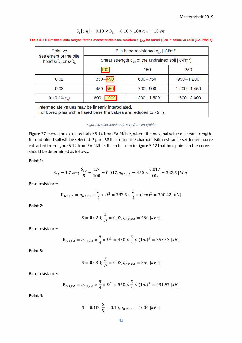
Masterarbeit 2019
43
Sg[𝑐𝑚] = 0.10 × 𝐷𝑏 = 0.10 × 100 𝑐𝑚 = 10 𝑐𝑚
Figure 37: extracted table 5.14 from EA Pfähle
Figure 37 shows the extracted table 5.14 from EA Pfähle, where the maximal value of shear strength
for undrained soil will be selected. Figure 38 illustrated the characteristic resistance-settlement curve
extracted from figure 5.12 from EA Pfähle. It can be seen in figure 5.12 that four points in the curve
should be determined as follows:
Point 1:
Ssg = 1.7 𝑐𝑚; 𝑆𝑠𝑔
𝐷=
1.7
100= 0.017, 𝑞𝑏,𝑘,𝐸𝐴 = 450 ×
0.017
0.02= 382.5 [𝑘𝑃𝑎]
Base resistance:
Rb,k,EA = 𝑞𝑏,𝑘,𝐸𝐴 ×𝜋
4× 𝐷2 = 382.5 ×
𝜋
4× (1𝑚)2 = 300.42 [𝑘𝑁]
Point 2:
S = 0.02D; 𝑆
𝐷= 0.02, 𝑞𝑏,𝑘,𝐸𝐴 = 450 [𝑘𝑃𝑎]
Base resistance:
Rb,k,EA = 𝑞𝑏,𝑘,𝐸𝐴 ×𝜋
4× 𝐷2 = 450 ×
𝜋
4× (1𝑚)2 = 353.43 [𝑘𝑁]
Point 3:
S = 0.03D; 𝑆
𝐷= 0.03, 𝑞𝑏,𝑘,𝐸𝐴 = 550 [𝑘𝑃𝑎]
Base resistance:
Rb,k,EA = 𝑞𝑏,𝑘,𝐸𝐴 ×𝜋
4× 𝐷2 = 550 ×
𝜋
4× (1𝑚)2 = 431.97 [𝑘𝑁]
Point 4:
S = 0.1D; 𝑆
𝐷= 0.10, 𝑞𝑏,𝑘,𝐸𝐴 = 1000 [𝑘𝑃𝑎]

Masterarbeit 2019
44
Base resistance:
Rb,k,EA = 𝑞𝑏,𝑘,𝐸𝐴 ×𝜋
4× 𝐷2 = 1000 ×
𝜋
4× (1𝑚)2 = 785.40 [𝑘𝑁]
Figure 38: extracted figure 5.12 from EA Pfähle
With the base and shaft resistance above, the total axial compression resistance can be sorted as follows. Determination of characteristic axial pile resistance according to EA-Pfähle section 5.4.6: Point 1:
Ssg = 1.7 𝑐𝑚; 𝑆𝑠𝑔
𝐷= 0.017,
Base resistance: Rb,k,EA = 300.42 [𝑘𝑁]
Shaft resistance: Rs,k,EA = 2406.81 [𝑘𝑁] Total compression resistance: Rc,k,EA = Rb,k,EA + Rs,k,EA = 300.42 + 2406.81 = 2707.23 [𝑘𝑁] Point 2:
S = 0.02𝐷; 𝑆
𝐷= 0.02,
Base resistance: Rb,k,EA = 353.43 [𝑘𝑁] Shaft resistance: Rs,k,EA = 2406.81 [𝑘𝑁]
Total compression resistance: Rc,k,EA = Rb,k,EA + Rs,k,EA = 353.43 + 2406.81 = 2760.24 [𝑘𝑁] Point 3:
S = 0.03𝐷; 𝑆
𝐷= 0.03,
Base resistance: Rb,k,EA = 431.97 [𝑘𝑁]
Shaft resistance: Rs,k,EA = 2406.81 [𝑘𝑁] Total compression resistance: Rc,k,EA = Rb,k,EA + Rs,k,EA = 431.97 + 2406.81 = 2838.78 [𝑘𝑁] Point 4:
S = 0.1𝐷; 𝑆
𝐷= 0.10,
Base resistance: Rb,k,EA = 785.40 [𝑘𝑁] Shaft resistance: Rs,k,EA = 2406.81 [𝑘𝑁] Total compression resistance: Rc,k,EA = Rb,k,EA + Rs,k,EA = 785.40 + 2406.81 = 3192.21 [𝑘𝑁]

Masterarbeit 2019
45
Figure 39: characteristic pile base, shaft and total compression resistance-settlement curve according to EA Pfähle
The characteristic pile resistance-settlement curve according to EA Pfähle is shown in Figure 39 above.
A1.1.2. Analytical method of Lang et al. (2011)
Determination of characteristic shaft resistance for undrained conditions according to Lang et al.
(2011):
For undrained conditions, the characteristic shaft resistance is acquired as follows:
Rs,k,Lang = 𝑈 × 𝐿 × 𝑆 = 3.14 𝑚 × 15 𝑚 × 70 𝑘𝑃𝑎 = 3297 [𝑘𝑁]
Where:
𝑈: circumference of the pile: 𝑈 = 𝜋 × 𝐷 = 𝜋 × 1 𝑚 = 3.14 [𝑚];
𝑆: shear strength between pile and soil: 𝑆 = 0.7 × 100 𝑘𝑃𝑎 = 70 [𝑘𝑃𝑎];
𝐿: pile length: 𝐿 = 15 [𝑚]
Determination of characteristic base resistance for undrained conditions according to Lang et al.
(2011):
Rb,k,Lang = 𝐴 × 𝑁𝑐 × 𝑆𝑢 = 0.25 𝑚2 × 9 × 100 𝑘𝑃𝑎 = 225 [𝑘𝑁]
Where:
𝑁𝑐: load capacity factor: 𝑁𝑐 = 9 𝑤𝑖𝑡ℎ 𝐿
𝐷=
15𝑚
1𝑚= 15 [−];(Figure 40)
𝐴: cross section area: 𝐴 =1
4× 𝜋 × 𝐷2 =
1
4× 𝜋 × (1𝑚)2 = 0.25 [m2];
𝑆𝑢: undrained shear strength: 𝑆𝑢 = 100 [𝑘𝑃𝑎]
Determination of total characteristic compression resistance for undrained conditions according to
Lang et al. (2011):

Masterarbeit 2019
46
Rc,k,Lang = 𝑅𝑠,𝑘,𝐿𝑎𝑛𝑔 + 𝑅𝑏,𝑘,𝐿𝑎𝑛𝑔 = 3297 + 225 = 3522 [kN]
Figure 40: load capacity factor according to Lang et al. (2011)
A1.2. Determination of vertical tension capacity for single pile
Section A1.1 has already shown the shaft and base resistance from both EA Pfähle and Lang et al.
(2011). For determination of compression resistance, both shaft and base resistance should be
counted. However, for case of tensive pile, only shaft resistance needs to be considered.
A1.1.1. Empirical method of “recommendation on piling (EA-Pfähle)”
Determination of characteristic tensive resistance according to EA-Pfähle section 5.4.6: Point 1:
Ssg = 1.7 𝑐𝑚; 𝑆𝑠𝑔
𝐷= 0.017,
Shaft resistance: Rs,k,EA = 2406.81 [𝑘𝑁]
Total tensive resistance: Rt,k,EA = Rs,k,EA = 2406.81 [𝑘𝑁] Point 2:
S = 0.02𝐷; 𝑆
𝐷= 0.02,
Shaft resistance: Rs,k,EA = 2406.81 [𝑘𝑁]
Total tensive resistance: Rt,k,EA = Rs,k,EA = 2406.81[𝑘𝑁] Point 3:
S = 0.03𝐷; 𝑆
𝐷= 0.03,
Shaft resistance: Rs,k,EA = 2406.81 [𝑘𝑁] Total tensive resistance: Rt,k,EA = Rs,k,EA = 2406.81 [𝑘𝑁] Point 4:

Masterarbeit 2019
47
S = 0.1𝐷; 𝑆
𝐷= 0.10,
Shaft resistance: Rs,k,EA = 2406.81 [𝑘𝑁] Total tensive resistance: Rs,k,EA = Rs,k,EA = 2406.81 [𝑘𝑁]
A1.1.2. Analytical method of Lang et al. (2011)
Determination of characteristic tensive resistance for undrained conditions according to Lang et al.
(2011):
R𝑡,k,Lang = 𝑅𝑠,𝑘,𝐿𝑎𝑛𝑔 = 3297 [kN]
A2. Hand calculation for pile group In this section the rotation of the pile group with the method of GAZETAS (1991) will be introduced.
The selected pile group in chapter 7 for lateral pushover analysis is 3-by-1. Due to the presence of a
pile cap, the acting moment is transferred to the piles through axial forces at the 2 edge piles and
through concentrated moments at the 9 pile heads. The rotation of the pile group is therefore
limited both by the rotational stiffness of each pile and the vertical stiffness of the two edges piles.
The rotational stiffness of a single pile in homogeneous soil is
KMM,SP = 0.15 × 𝐸𝑠 × 𝐷3 × (𝐸𝑝
𝐸𝑠)
0.75
= 0.15 × 18 𝑀𝑃𝑎 × (1 𝑚)3 × (31′000 𝑀𝑃𝑎
40 𝑀𝑃𝑎)
0.75
= 396.59 𝑀𝑁𝑚/𝑟𝑎𝑑
The vertical stiffness of the single pile is calculated according to Randolph & Wroth (1978).
Figure 41: shearing modulus distribution according to Randolph & Wroth (1978)
𝑃
𝑤= 𝐺𝐿𝑟0
4𝑛(1 − 𝑣)𝜉
+2𝜋𝜌
𝜁 ×tanh (𝜇𝐿)
𝜇𝐿 ×𝐿𝑟0
1 +1
𝜋𝜆×
4𝑛(1 − 𝑣)𝜉
×tanh (𝜇𝐿)
𝜇𝐿 ×𝐿𝑟0
Where:
ν: Poisson’s ratio of the soil ν = 0.3

Masterarbeit 2019
48
𝐺𝐿: shear modulus of soil constant with depth: 𝐺𝐿 =𝐸𝑠
2(1+ν)=
18 𝑀𝑃𝑎
2(1+0.3)= 6.92 𝑀𝑃𝑎
𝐺𝑏: shear modulus at pile base: 𝐺𝑏 = 𝐺𝐿 = 6.92 𝑀𝑃𝑎
𝜉: ratio of end-bearing: 𝜉 =𝐺𝐿
𝐺𝑏= 1
𝜌: variation of soil shear modulus with depth: 𝜌 =𝐺𝐿/2
𝐺𝐿= 1
𝑟𝑚: radius of influence of pile: 𝑟𝑚 = 𝐿 × (0.25 + 𝜉(2.5𝜌(1 − ν) − 0.25)) =
15 m × (0.25 + 1 × (2.5 × 1 × (1 − 0.3) − 0.25)) = 26.25 m
𝜁: measure of radius of influence of pile: 𝜁 = ln (𝑟𝑚
𝑟0) = ln (
26.25 𝑚
0.5 𝑚) = 3.96 [−]
𝜆: pile-soil stiffness ratio: 𝜆 =𝐸𝑝
𝐺𝐿=
𝐸𝑐
𝐺𝐿=
31′000 𝑀𝑃𝑎
6.92 𝑀𝑃𝑎= 4479.77 [−]
𝜇: measure of pile compressibility: 𝜇 =1
𝑟0√
2
𝜁𝜆=
1
0.5 𝑚√
2
3.96×4479.77= 0.021
n: ratio of underream: n =𝑟𝑏
𝑟0= 1
𝑃
𝑤= 𝐺𝐿𝑟0
4𝑛(1 − 𝑣)𝜉
+2𝜋𝜌
𝜁 ×tanh(𝜇𝐿)
𝜇𝐿 ×𝐿𝑟0
1 +1
𝜋𝜆×
4𝑛(1 − 𝑣)𝜉
×tanh(𝜇𝐿)
𝜇𝐿 ×𝐿𝑟0
= 6920 𝑘𝑃𝑎 × 0.5 𝑚 ×
4 × 1(1 − 0.3) × 1
+2𝜋 × 1
3.96 ×tanh(0.021 × 15 𝑚)
0.021 × 15 𝑚×
15 𝑚0.5 𝑚
1 +1
𝜋 × 4479.77 ×4 × 1
(1 − 0.3) × 1×
tanh(0.021 × 15 𝑚)0.021 × 15 𝑚
×15 𝑚0.5 𝑚
= 177′139 kN/m
The vertical stiffness of the single pile is then:
Kv,SP =𝑃
𝑤= 177′139 kN/m
The total rotational stiffness of the pile group is:
Kr = 2 × 𝑠2 × Kv,SP + 3 × KMM,SP = 2 × (3 𝑚)2 × 177.139𝑀𝑁
𝑚+ 3 × 396.59
𝑀𝑁𝑚
𝑟𝑎𝑑
= 4′378.272 𝑀𝑁𝑚
𝑟𝑎𝑑
Finally, the average rotation of the rigid pile cap under the characteristic moment action for a
serviceable limit calculation:
θb =𝑀𝑘
𝐾𝑟=
𝑀𝑘
4′378.272 𝑀𝑁𝑚𝑟𝑎𝑑

Masterarbeit 2019
49
Appendix B In Appendix B, the details and workflow of Abaqus Plugin will be clearly explained, as supplementary
explanation for chapter 5 and 6. The whole workflow of the developed python script is already
illustrated in Figure 23 in chapter 6. In this appendix, the automatic input file generation of both MC
and CDP pile will be clearly and detailly explained.
B1: Design structure and workflow of python script As is shown in Figure 42, the user can give the dimensions of pile, cap and soil respectively, and then
the script reads the input parameters from user and works as shown on the right hand side of Figure
42.
At first, the parts of both pile and soil will be created, respectively. In order to control the mesh,
partitions will be implemented after parts generation. Then, the seed will be conducted accurately
after partition to make sure the mesh is accurate and proper enough. With all the pre-processing
work done above, the model mesh will be generated and the whole is divided into fine finite
elements. In order define elements’ properties later, the elements sets will be deliberately selected
and saved. After the material input, the whole model’s input file can be generated.
The input file, generated automatically from Abaqus, is always not clean enough. It contains a lot of
useless information and will make the whole input file very hard to read and understand. Thus, the
extraction of useful information from the system input file is highly necessary. The information of
nodes and elements will be firstly extracted for further reproduction of a clear input file. Finally, the
clean and comprehensible input file will be generated, for final static analysis.
Figure 42: User interface and workflow of the python script
The details of all the workflow in Figure 42 are shown as follows from B1.1 to B1.11.
B1.1. Introduction to Abaqus RSG dialog builder Abaqus has a built-in plugin development tool, called “Really Simple GUI (RSG) Dialog Builder” Figure
43.

Masterarbeit 2019
50
Figure 43: Abaqus built-in plugin development tool (RSG dialog builder)
The final user dialog in shown in Figure 42, where text field, radio button, check button, label,
vertical aligner and color button are used. All the functions of them are listed below:
i. Text field: a text entry field that can be set to accept text, integers, or floats
ii. Radio button: an option button that can be set on or off; only one radio button at a time in a
group may be on
iii. Check button: an option button that can be set on or off
iv. Label: read only text
v. Vertical aligner: an invisible frame around a group of widgets that are displayed in a vertical
layout with the left edge of their text field aligned
vi. Color button: a button that posts the selected color dialog
After the creation of UI, the kernel option in Figure 43 will be used to load python script (Figure 44).
Thus, the next step is to write the python script firstly and load it into the kernel module field. After
that, a plugin file which can be added into Abaqus plugins file path is successfully created.
Figure 44: Kernel option in RSG dialog builder to load python script

Masterarbeit 2019
51
B1.2. Abaqus macro and python programming language
Abaqus/CAE is a complete Abaqus environment that provides a simple, consistent interface for
creating, submitting, monitoring, and evaluating results from Abaqus/Standard and Abaqus/Explicit
simulations (SIMULIA, 2009).
In order to have access to all the macro codes of Abaqus, the Abaqus built-in macro manager (Figure
45) is used, so that a python script can be written afterwards to do the modelling automatically. This
workflow means the macro will record all the manual operations during modelling and show the
macros directly in a script. Most of the manual operations can be used to generate the final python
script. However, some specific functions, e.g. selecting the lines, faces or element sets, cannot be
realized again by using Abaqus macro. Thus, customized algorithms should be developed, by using
Abaqus macro function library.
Figure 45: Abaqus macro manager
The script language used in Abaqus plugin is python, which is an interpreted, high level, general-
purpose programming language. Created by Guido van Rossum and first released in 1991, python’s
design philosophy emphasizes code readability with its notable use of significant whitespace. Abaqus
has chosen python as its admissive programming language. After the brief introduction of Abaqus
plugin above, the numerical modeling process controlled by Abaqus macro is listed in the following
sections.
B1.3. Create part of pile and soil
The first step of pre-processing of finite element model is creation of parts. As is already illustrated in
appendix A, two kinds of pile, MC (moment curvature) pile and CDP (concrete damaged plasticity)
pile, are employed for comparison and static analysis.
In the first step “create part”, the macro’s function used in both piles are the same (Figure 46). As is
shown in Figure 46, the function used for creation of soil part and pile part are different, although
they are both extrusion solids. The plane of soil used for extrusion is a rectangle (determined by two
points), while for pile is a circle (determined by one circle center and one point in the circle). After
the extraction of rectangle for soil part, holes in the soil corresponding to pile size and position are
cut for piles to be put into. The size and position of holes should be the same as those of piles (circle
plane and depth), so that the subsequent processing of pile and soil interface can be successfully
conducted.

Masterarbeit 2019
52
Figure 46: Abaqus macro functions for creation of model and part
B1.4. Create partition
After part generation in section B1.3, the partition soil and pile parts are shown in this section, for
accurate mesh control of the whole model. The datum plane is used here for partition. The soil and
pile models can be accurately cut by used the selected datum plane (e.g. XY, YZ, XZ plane). The macro
functions used here are shown in Figure 47.
Figure 47: Abaqus macro function for partition of soil and pile
It should be mentioned here that the fine mesh areas around piles for MC & CDP pile are different.
MC pile itself has a relatively coarser mesh than CDP pile. Thus, for MC pile, the fine mesh area in soil
is also relatively smaller than that for CDP pile. As is shown in Figure 48, the partition datum plane for
MC pile is 1 diameter beside the pile center (Figure 48 (a)), while that for CDP pile is 1.5 diameters
(Figure 48 (b)).

Masterarbeit 2019
53
Figure 48: Partition datum plane around pile for (a) MC & (b) CDP pile
The partition size in Z direction for pile is shown in Figure 49. There is an XY partition datum plane,
which stays 1 pile diameter above the pile base. This partition is specially processed for finer mesh
against the parts above. As the pile base and the soil around pile base are relatively sensitive to mesh
size. The pile end bearing resistance has a strong relationship with the soil around pile base (Figure
50).
Figure 49: Partition size of pile
The pile base resistance mechanisms (Figure 50) developed so far depend highly on the soil below
and even above the pile base. Thus, for both pile and soil, the relatively finer mesh is conducted 1
diameter above the pile base.

Masterarbeit 2019
54
Figure 50: Pile end bearing resistance mechanism
B1.5. Seed
After the partition of soil and pile model, the fine and accurate mesh will be achieved by seed. In
general, there are two types of seed in Abaqus: seed by number and seed by size. The Abaqus system
macro cannot record the coordinates of the line to be seeded. Thus, the edges should be selected at
first by using function “findAt()”. The input parameters in this function is a point coordinates (X, Y, Z).
If the point in within the line, the line will then be selected. All the algorithm in part B2 are based on
this method.
Figure 51: Abaqus macro functions for control of seed in soil part above pile base
The seed of soil along the direction of depth is divided into three parts. For seed above pile base
(from soil surface to one diameter above pile base), it can be seen in Figure 51 that the mesh size if
0.5 pile diameter. Here the mathematic function “ceiling” is used, for non-integer cases. E.g. 9.9
divided by 0.5 is 20. This method makes sure the mesh size is uniformly distributed, even if the input
soil depth from user is non-integer.

Masterarbeit 2019
55
Figure 52: Abaqus macro functions for control of seed 1 diameter above pile base
The mesh of underpart of soil is relatively finer than upperpart. As is shown in Figure 52, the mesh in
the area of 1 diameter above pile base is 0.25 pile diameter, namely seeded by size 4 (Figure 52). The
reason of finer mesh in this area is introduced in B1.4.
Figure 53: Abaqus macro functions for control of seed below pile base
Figure 53 shows the seed in soil below pile base. The size is set to 0.25 diameter of pile and the
mathematic method “ceiling” is used again for non-integer cases.

Masterarbeit 2019
56
Figure 54: Abaqus macro functions for control of seed on soil surface (outer edges)
After the pre-processing of seed along soil depth, the seed on the soil surface is shown in Figure 54
and Figure 55. The outer edges of the soil surface are seeded by size of 0.5 pile diameter (Figure 54),
while the inner edges are seeded by size of 0.25 diameter. For inner edges around pile, the seed is
specifically controlled by number 2 or 3 (Figure 55 and Figure 56) to make the mesh proper enough,
to avoid mis-convergence during calculation and let the computer calculate the finite element model
more efficiently.
Figure 55: Abaqus macro functions for control of seed on soil surface (inner edges)

Masterarbeit 2019
57
Figure 56: Abaqus macro functions for control of seed in area around pile
After the seed control in soil (from Figure 51 to Figure 56), the seeds on the pile along pile depth are
illustrated in Figure 57. Same as the seed on soil, the upper part of pile is seeded by size of 0.5 pile
diameter, where non-integer case (input pile depth) is also considered by using mathematic method
“ceiling”. The underpart of the pile (1 pile diameter above pile base) is seeded by number of 4 (0.25
pile diameter). The seed on pile coincide quite well with the seed on soil. Thus, the further pile-soil
interaction properties can be successfully determined, using the perfect match of pile and soil mesh.
This means all the nodes on pile surface shares the same coordinates with those on the soil surface.
Abaqus can recognize those nodes and find the surface automatically, which makes further
processing of pile-soil friction force more straightforward.
Figure 57: Abaqus macro functions for control of seed along pile depth
It should also be mentioned that the mesh on the head of the pile is shown on the right-hand side in
Figure 56. In x direction, it is divided by number of 2 and y direction by 3. The curve is also divided by
3.
B1.6. Generate mesh
After the pre-processing from B1.1 to B1.5, the model can be meshed. Figure 58 shows an example
of a 3-by-2 pile group foundation with cap and pier above. It can be seen clearly in Figure 58 that the

Masterarbeit 2019
58
upperpart of the soil model has a relatively coarser mesh than underpart. Moreover, the mesh in
inner area near the pile group is also finer than that in outer area.
Figure 58: A mesh example of a 3-by-2 pile group foundation with cap and pier above
With the meshed model above, the nodes and elements generated can be managed for specific
purpose in the following sections.
B1.7. Sets management
Figure 59: Abaqus macro functions for sets management
As is shown in section B1.6, all the nodes and elements are available after mesh. By using the
intrinsic function “getByBoundingBox” (Figure 59), the elements inside the given bounding box can
be selected for specific uses (e.g. definition of elements’ material).
B1.7.1. Sets management for material definitions
In the script, every 1 m soil elements are selected as a unique element set (Figure 59), for further
definition of each layer’s material properties. This is quite helpful when dealing with complex and
non-homogenous soil layers (e.g. alluvial deposit on the surface, soft soil below and stiff rock on the

Masterarbeit 2019
59
base). The selected soil element sets enable a relatively flexible material definition for further
research.
B1.7.2. Sets management for control of boundary conditions
The nodes can not only be acquired with bounding box method, but also with selected faces after
step “create part”. After the creation of soil and pile part, the soil faces can be selected by using
Abaqus macro function “findAt()”. The input parameter of this function is a node’s coordinate inside
the face (Figure 59). The faces can be pre-selected and meshed afterwards. When controlling the
boundary conditions of the soil element, these faces can be used for management of node sets. It
can be clearly seen in Figure 59 that all the surfaces’ nodes in both x and y direction (faceSide-X &
faceSide-Y), and the soil base surface nodes are selected for boundary condition control as follows.
Figure 60: Constrain of x-direction for soil model
Figure 60 to Figure 62 have shown the boundary conditions of the soil model. The boundaries of the
soil model should be strictly constrained, so that the whole model can be statically determinate. It
can be seen in Figure 60 and Figure 61 that peripheral surfaces of the soil model are fixed against
further extension and shrink in x and y direction, respectively. In Figure 62, the soil model’s z
direction is also fixed against rappelling and ascending. Moreover, x direction of the base is also fixed
to avoid horizontal movement.
Figure 61: Constrain of y-direction for soil model

Masterarbeit 2019
60
Figure 62: Constraints of base for soil model
It should be mentioned that the boundary constraints are applied directly to the node sets. The
Abaqus input keyword “BOUNDARY” invokes the function, where node sets and constrained
directions should be given.
B1.7.3. MPC (multi-point constraints) connection
Besides element selection and boundary control, the connection between specific nodes is also
inevitable during pre-processing.
B1.7.3.1. MPC connections on pier
As is shown on the right-hand side in Figure 58, the base node of the pier has a master control over
all the nodes on cap surface. Moreover, the top node of the pier controls all other beams nodes in
the pier. As is shown in Figure 63, the top node on the pier controls all other nodes, which means the
lateral pushover load added at the top node will drive all the “slave” nodes move at the same pace.
This method makes the further lateral pushover analysis more accurate, as the relative horizontal
displacement between pier top and base is zero. Only rotation will be counted in. This means the
moment added on the pile group is can be simplified as lateral load multiply pier height, which also
makes the extraction of moment and rotation angle afterwards easier. The rotation angle can be
extracted directly by selecting the pier base node in Abaqus ODB result file.
Figure 63: Example for multi-point constraints connection of pier

Masterarbeit 2019
61
B1.7.3.2. MPC connections in MC pile
The modelling of MC (moment curvature pile) is mainly based on multi-point connections. The
nonlinear beam elements (Figure 64) controls each layer’s nodes. The master nodes are the beam
nodes, and the slave nodes are the surrounding nodes around the beam nodes.
The hybrid modelling of this MC pile consists of two parts. One part is the pseudo continuum
elements around the beam elements. Those pile elements have no density, stiffness and poison
ratio. What they offer is the well-matched pile nodes around the beams in the middle. Another part
of the hybrid modelling is the beam element in the middle. Those beam elements control the
surrounding nodes in their layer and drive the nodes move up and down at the same pace.
Figure 64: MPC connections in MC pile
B1.7.3.3. MPC connection between pile head and pile cap for MC pile
Figure 65: MPC connection between MC pile and cap
The connections between pile head and cap is also very important. For case MC pile, the top node on
the beam masters all the nodes, which match the mesh of pile on pile cap bottom surface (Figure 65).
It can also be found in Figure 65 that the top master node of the beam in MC pile controls two node

Masterarbeit 2019
62
sets, one set on pile cap bottom surface and one on pile top surface. These two node sets share the
same coordinates and stay in the same position. The top node is a connection between these two
node sets. Once the pile cap moves, the pile below will also be driven due to these multi-points
connections.
B1.7.3.4. MPC connection between pile head and pile cap for CDP pile
The connections between pile head and cap for CDP pile are different from those for MC pile. For
CDP pile group with pile cap above, there is no MPC connections in CDP piles. The node set of pile
Figure 66: MPC connection between CDP pile and cap
top is slave set to node set at cap surface (Figure 66). It can be seen in Figure 66 that these two node
sets have one-to-one node connection. The mechanism of CDP pile is introduced in Figure 67. It can
be clearly seen in Figure 67 that one CDP pile consists of three different parts: unconfined concrete
Figure 67: Element sets for CDP pile
elements, confined concrete elements and reinforcement respectively. These three parts are
assembled into one pile, which means the nodes on the surfaces of reinforcement, inner confined
concrete and outer unconfined concrete share the same coordinates. The exact material definition
of CDP pile will be illustrated in section B1.8.

Masterarbeit 2019
63
B1.8. Material input
Figure 68: Abaqus macro functions for material definition and moment curvature for MC pile
With the sets created above, the materials, e.g. density, elastic modulus and poison ratio, should be
defined by using the macro functions in Figure 68.
B1.8.1. Materials of MC pile
As is already discussed in section B1.7, MC pile consists of beam elements and pseudo pile elements.
The pile elements have no density, elastic modulus and poison ration. However, the beam elements
in the middle have user-defined properties.
As is shown in Figure 68, the bending moment curvature of the beam is acquired by the following
preconditions for pile and cap.
• Precondition 1: The vertical axial load remains constant during lateral push-over analysis.
• Precondition 2: The diameter of the pile is 1m and reinforcement ratio is 1%
• Precondition 3: This is a 3-by-1 pile group with an 8mX2mX1m pile cap (Figure 69)
Figure 69: Dimension of the 3-by-1 pile group’s cap for lateral pushover analysis
The pier on the pile cap has a diameter of 1.5m and height of 6m. Thus, the axial load added on the
single pile is uniformly distributed as follows:

Masterarbeit 2019
64
𝑁𝑣𝑒𝑟𝑡𝑖𝑐𝑎𝑙 =𝐺𝑝𝑖𝑒𝑟 + 𝐺𝑐𝑎𝑝
𝑁𝑝𝑖𝑙𝑒
Where:
Nvertical: axial load added on single pile
Gpier: weight of pier
Gcap: weight of cap
Npile: number of piles
With the constant axial load added on the pile, the moment curvature is acquired with Fagus (a static
analysis software). It should be mentioned that the axial load for single pile is also from the equation
above. However, the weight of cap and pier should be adjusted. Thus, the moment curvature for
single pile is different from that for pile group. The soil parameters, together with the concrete
parameters used for pile, cap and pier, are shown in Table 3.
Table 3: Soil and concrete parameters
Elastic modulus Density Poison ratio
Unit [MPa] [kN/m^3] [-]
Soil 18 16 0.3
Concrete 31000 25 0.1
B1.8.2. Materials of CDP pile
As is already shown in Figure 67, a CDP pile consists of three parts, namely confined inner concrete,
reinforcement in between and outer unconfined concrete. Although the confined and unconfined
concrete have the same elastic modulus and poison ratio, the constitutive laws are distinguishing due
to the “confined effect”. The inner concrete is strictly confined by the reinforcement, which indicates
that the compression and tension yield stress and the stress development curve is totally different
from unconfined normal concrete. Thus, the constitutive properties of both concrete types should be
defined separately, to accurately simulate the real concrete pile.
B1.8.2.1. Confined concrete
Figure 70: (a) Compression stress-strain curve of concrete and (b) confined concrete crushing curve (stress-inelastic strain curve)

Masterarbeit 2019
65
Figure 70 (a) shows the normal constitutive curve of concrete. It is normally divided into two stages:
elastic and inelastic stage. For elastic stage before yield point on the curve, the compression stress-
strain curve shows linear increment, whose derivative is the concrete elastic modulus used in Table 3
(31GPa). This elastic modulus applies to confined and unconfined concrete. For stage after yield
point, inelastic compression stress-strain curve is shown in Figure 70 (b). This curve shows the
crushing of concrete with increasing inelastic strain. The concrete type is C30/37. It can be seen
clearly in Figure 70(b) that inelastic strain increases rapidly after the compression stress reaches a
summit of 38MPa. The “confined effect” on the inner concrete has enlarged the real compression
strength. With these two stages’ compression stress-strain relationship, the confined concrete’s
constitutive laws constitutive law is determined.
After the determination of constitutive law for confined concrete, the cracks development in
concrete with increasing inelastic strain is also crucial for further damage analysis. Figure 71 shows
the compression cracks development with increasing inelastic strain. It can be seen in Figure 71 that
the ultimate turning point occurs when inelastic strain reaches 14‰. It should be mentioned that the
damage in Figure 71 has no unit, only a magnitude, which is specially designed for describing cracks’
development vividly.
Figure 71: Confined concrete compression cracks development curve with increasing inelastic strain
After the determination of compression stress-strain relationship for confined concrete, the normal
tension stress-strain curve is shown in Figure 72. It can be seen clearly in Figure 72 (a) that the
tension stress-strain curve is also divided into two parts: elastic and inelastic part. For elastic stage,
the tension stress in concrete develops linearly with increasing elastic strain, where the elastic
modulus is the same as that for compression case in Figure 70. After the summit, where tension
stress is around 1.8MPa, the tension stress in concrete decreases with increasing inelastic strain. In
this inelastic stage, crack occurs, and inelastic strain increases rapidly (Figure 72 (b)). Figure 72 (b)
shows the second stage of the tension stress-strain curve in Figure 72(a).
Figure 73 illustrates the tension cracks development with increasing inelastic strain. Different from
the crack’s development for compression case (Figure 71), the crack for tension case occurs at a
relatively earlier stage. For same damage of 0.8, the compression inelastic strain is 14‰ in Figure 71,
while the tension inelastic strain in Figure 73 shows a much smaller value of 0.18‰. This is mainly
due to the concrete character, which has a large compression resistance but a much smaller tension
resistance. Tension crack occurs at a very early stage.

Masterarbeit 2019
66
Figure 72: (a) Tension stress-strain curve of concrete and (b) confined concrete tension curve (stress-inelastic strain curve)
It should also be mentioned in Figure 73 that the tension damage curve has no plateau, in
comparison to that from compression case (Figure 71). This indicates the tension cracks development
is relatively “brittle” and shows a relatively weak “ductility” than that for compression case.
Figure 73: Confined concrete tension cracks development curve with increasing inelastic strain

Masterarbeit 2019
67
B1.8.2.2. Unconfined concrete
Figure 74: (a) Compression stress-strain curve of concrete and (b) unconfined concrete crushing curve (stress-inelastic strain curve)
After the determination of material properties for confined concrete, unconfined concrete is also
shown in Figure 74. The concrete type here is C30/37, which coincides well with the summit in Figure
74 (b). The unconfined concrete is outside the reinforcement, where no confinement is added on the
concrete. Thus, the concrete strength is not influenced by the surrounding materials at all.
Figure 75: Unconfined concrete compression cracks development curve with increasing inelastic strain
Similar to confined concrete, the inelastic stress-strain curve in Figure 74 (b) corresponds to the
inelastic part in Figure 74 (a). After reaching the summit where the compression stress is 30 MPa, the
inelastic strain drops down rapidly. It should be mentioned here that the elastic modulus used here is
the same as that for confined concrete. The elastic modulus is shown in Table 3.
The crack’s development curve with increasing inelastic strain is shown in Figure 75. Different from
the curve in Figure 71, the compression damage curve in Figure 75 reaches no plateau when the
damage comes to 0.8 and the inelastic strain at this point (6.2‰) is relatively smaller than that
(14‰) in Figure 71. This indicates that the cracks’ development is constrained due to the

Masterarbeit 2019
68
confinement. The unconfined concrete outside the reinforcement shows a relatively quicker cracks’
development at the same inelastic strain.
Figure 76: (a) Tension stress-strain curve of concrete and (b) unconfined concrete tension curve (stress-inelastic strain curve)
After the determination of concrete compression constitutive law above, the tension stress-strain
relationship is also illustrated in Figure 76. It should be mentioned in Figure 76 that the tension
stress-inelastic strain curve (Figure 76 (b)) corresponds to the right part of the tension stress strain
curve in Figure 76 (a). In Figure 76 (a), the tension stress shows a linear increment with increasing
strain before reaching the summit. After the summit, the tension stress decreases rapidly with the
increasing inelastic strain. The tension stress-strain curve for the second stage is shown Figure 76 (b).
Figure 77: Unconfined concrete tension cracks development curve with increasing inelastic strain
The tension cracks’ development with inelastic strain for unconfined concrete outside the
reinforcement is demonstrated in Figure 77. When comparing Figure 77 with Figure 75, it can be
clearly found that the concrete reaches a much earlier tension damage than compression case. For
cracks development to a value of 0.8 in tension case (Figure 77), the inelastic strain is only 0.18‰.
This inelastic strain corresponds to nearly no damage in concrete for compression case in Figure 75.

Masterarbeit 2019
69
It is mainly due the concrete’s character: the tension resistance is much smaller than the
compression resistance.
With all the constitutive properties defined above, the concrete material is properly determined for
CDP pile. The reinforcement between the confined and unconfined concrete should be determined
as follows.
B1.8.2.3. Reinforcement
The reinforcement in the concrete is simulated as shell element. Parameters of the reinforcement
are listed as follows:
Table 4: parameters of reinforcement used in CDP pile
Value Unit
Elastic modulus 210 [GPa]
Poison ratio 0.3 [-]
Density 78.5 [kN/m^3]
Details of defining the reinforcement are shown in section B1.11.2.4 in Appendix B.
B1.8.3. Materials of soil
Table 2 has already shown the basic properties of soil used in this thesis. Beside those basic
properties, the failure mechanism is determined as follows.
For soil failure mechanism, the modified von-mises failure criteria is selected, instead of Mohr-
Coulomb failure criteria, to simulate the soil failure behavior. Although Mohr-Coulomb failure criteria
provides a good fit to the experimental data in triaxial compression and extension, it is not the most
convenient model to use, either for analytical or numerical analysis (Puzrin (2012)).
For analytical analysis with Mohr-Coulomb failure criteria, the analytical derivations, based on the
complex expression of failure surface in the stress tensor invariant space, are extremely complicated.
For numerical case, the numerical analysis may easily run into difficulties, as the surface in 3D
principal stress space is not “smooth”, it has “corners” (Figure 19).
Those difficulties are eliminated by modified Von-Mises failure criteria. The surface of Von-Mises
failure criteria in 3D principal stress space is a cylinder in Figure 19. Details of the modifications can
be found in section 5.2 in chapter 5.

Masterarbeit 2019
70
B1.9. Generate input file
Figure 78: Abaqus macro functions for generation of input file
After all the pre-processing of the soil-pile model, the system input file can be automatically created
by using the macro functions shown in Figure 78. The system generated input file is contains all the
operations above, where all the information is gathered in the input file, even the operation
command. Thus, it is necessary to clean the needless information in the input file and retain the
useful information. The details are shown in the following section.

Masterarbeit 2019
71
B1.10. Extract useful information from input file
Figure 79: Python codes for extraction of useful information from system input file
Figure 79 shows the python codes for extraction of useful information from system generated input
file. For generation of a clean and understandable input file, what is useful in old input file is the
information of nodes and elements. The nodes and elements are miscellaneous and the data of them
are huge. Thus, the nodes and elements should be firstly extracted for preparation of a clean input
file. Other useful information like node and element sets should also be extracted afterwards. The
information of material definition and connection relationship can be written manually into the new
input file with the python code. The load cases are written directly into the input file as well. Thus,
the useful information here is the coordinates of nodes, nodes set, elements and elements’ sets.
With the pre-selected information above, the final input file can be created as follows.
B1.11. Final input file generation
This section illustrates the contents of the input file. Different from the system input file generated
from Abaqus CAE, this input file is written purposely for users to understand and modify. Thus, it
shows a much more understandable structure and clean content. The input files’ contents of MC and
CDP pile are listed separately as follows.
B1.11.1. Contents of input file for MC pile foundation
This section introduces the contents’ structure of input file for MC pile foundation. At the beginning,
nodes and elements of soil, piles, beams in piles, pile cap and pier will be determined as the basic
preparation for the following step: determination of connections between nodes. After the
determination of MPC (multi-point constraints) connection, the sections of soil, pile, beam, pile cap
and pier should be defined, and the corresponding materials will also be determined. Then the
boundary conditions should be processed for preparation of calculation. The final step is the
management of load cases and pushover analysis. Details of those processes are shown as follows:
B1.11.1.1. Determination of nodes and elements:
After mesh of parts for the whole model, nodes and elements are created. The definition of nodes
follows the following format:
First line: *NODE, NSET= name of node set to which these nodes will be assigned
Second line: Node number, first coordinate of the node, second coordinate of the node, third
coordinate of the node

Masterarbeit 2019
72
It should be mentioned that the coordinate systems used here is rectangular cartesian coordinate
systems. The length unit used for the whole system is meter.
B1.11.1.1.1. Soil
After the definition of soil nodes with the format above, special node sets should be selected for
further use. For boundary conditions’ control, the nodes on the side surfaces and base of the soil
should be selected (Figure 60, Figure 61 and Figure 62). The method to select nodes as a set is
already introduced in section B1.7. The format to define node set is shown as follows:
First line: *NSET, NSET=name of the node set to which the nodes will be assigned
Second line: list of nodes or node set labels to be assigned to this node set. Only previously
defined node sets can be assigned to another node set.
By using the input format above, the side nodes are selected as node sets with name “SIDES-X”,
“SIDES-Y” and “Base” respectively.
With the already defined nodes and node sets, the element and element set for soil should be
defined as well. In this thesis, the format to define elements by specifying their nodes are shown as
follows:
First line: *ELEMENT, TYPE=element type, ELSET=name of element set
Second line: element number, element nodes that define the element
This option is used to define an element directly by specifying its nodes.
Figure 80 shows the commonly used element families. The element type used for soil is continuum
(solid and fluid) elements. For continuum elements, displacements or other degrees of freedom are
calculated at the nodes of the element. At any other point in the element, the displacements are
obtained by interpolating from the nodal displacement. Usually the interpolation order is determined
by the number of nodes used in the elements.
Figure 80: Commonly used element families
Figure 81 shows three different types of continuum elements, namely linear, quadratic and modified
second-order element.

Masterarbeit 2019
73
As is shown in Figure 81 (a), elements have nodes only at their corners, which means linear
interpolation in each direction is used between two nodes. Thus, this kind of elements is called linear
elements or first-order elements. Different from the 8-node brick in Figure 81 (a), the 20-node brick
is shown in Figure 81 (b), with nodes in the middle. This kind of interpolation is quadratic
interpolation. These elements are therefore called quadratic elements or second-order elements.
Modified triangular or tetrahedral elements with midside nodes are shown in Figure 81 (c), with a
modified second-order interpolation. They are often called modified or modified second order
elements. The calculation efficiency decreases with increasing element orders. Thus, for convergence
of the whole model during calculation, the element type C3D8 (Figure 81 (a)) is selected for soil
elements. 8 nodes should be determined when defining the elements.(有时间这里介绍一下 C3D8
的性质)
Figure 81: Linear brick, quadratic, and modified tetrahedral elements
B1.11.1.1.2. Pile cap
To define the nodes of pile cap, the node number for pile cap should not collide with that for soil.
The nodes’ coordinates are extracted from Abaqus system input file (section B1.10), where the
nodes’ number of soil and other models like piles are always variable. This is mainly due to the
alteration of model dimension and mesh. The irregular node numbers make it difficult for users to
read and adjust the input file. Thus, it is necessary to set a rule for nodes’ numbering.
Due to the variance of soil nodes, the following mathematic method is used for selecting a decent
starting number for models after soil (e.g. pile cap).
labelMultipler = int(pow(10, len(str(soilNodeMax))))
curLabelMultipler += 1
labelStart = curLabelMultiple * labelMultipler
For example, if the last node number of soil model is 899991, the starting node number of the model
after soil (e.g. pile cap here) is 1000000. For model after pile cap, if the end node number of pile cap
is 1929332, the starting node number of the model (e.g. pier) is 2000000. By using this mathematic
method, the starting node number of all the models can be clearly found and easy to understand.
After the determination of nodes’ coordinates for pile cap, the nodes on the surface of pile cap
should be selected as a node set. This node set will be used for further MPC (multi-point constraints)
connections with pier. This part will be introduced in the following section. The format to define the
node set is already introduced in the aforementioned sections, where node sets in soil are defined.

Masterarbeit 2019
74
Same as the element type for soil, element type C3D8 is also selected for pile cap for the same
reason. The format to define elements for pile cap is the same as that for soil, with the nodes defined
above for pile cap.
B1.11.1.1.3. Pier
The nodes definition for pier is relatively simple than soil and piles. Pier is simulated as divided beam
elements. Each beam section length is 0.5 meters. The nodes at the top and at the base of the pier
are selected separately as node sets for further use (MPC connections).
B1.11.1.1.4. Pile
The element type for pile is eight-node brick element with reduced integration (C3D8R). Different
from C3D8, element type C3D8R is not stiff enough in bending. Moreover, the integration point of
C3D8R element is located in the middle of the element (Figure 82). For normal analysis of stresses,
strains, these values are accurate only in the integration points. Thus, small elements are required to
capture a stress concentration at the boundary of a structure.
Figure 82: 1X1X1 integration point scheme in hexahedral elements
B1.11.1.1.5. Beam in pile
Before the definition of beam elements in pile, the format of beam elements should be introduced at
first. Figure 83 shows the format of element type for beam element in Abaqus. Here B31 is used for
simulation of beams in the middle of pile. B31 means a beam in space that uses linear interpolation.
Figure 83: definition of beam element in Abaqus
The beam used here is the traditional Timoshenko beam, which allows for transverse shear
deformation. This kind of beam can not only be used for stout beam, but also for slender beam.
Moreover, the Timoshenko beams can be subjected to large axial strains. Thus, this beam type B31 is
selected for the numerical modelling.

Masterarbeit 2019
75
The format to define the beam element is shown as follows:
First line: *ELEMENT, TYPE = beam type, ELSET = name of element set
Second line: element number, first node number forming the element, second node number
forming the element
The beam elements are not pre-defined and generated in Abaqus. They are written manually using
python code. The length of the whole beam in the middle of pile should match the length of pile.
Moreover, the section length of each beam element should also match the mesh of pile and soil, so
that the nodes in the beam and pile coincide well with those in soil. The interface between pile and
soil can be properly processed later.
B1.11.1.2. Determination of connections
After the pre-processing of nodes and elements, the connections between nodes should be
conducted. Multi-point constraints (MPC) connection is commonly used in Abaqus by giving the
associated data. This kind of connection allow constraints to be imposed between different degrees
of freedom of the model and can be quite general (nonlinear and nonhomogeneous). The format of
the MPC connection used in this thesis is shown as follow:
First line: *MPC
Second line: connection type (BEAM here), slave node, master node
It should be mentioned that the connection type used in this thesis is “BEAM”, which provides a rigid
beam between two nodes to constrain the displacement and rotation at the first node to the
displacement and rotation at the second node, corresponding to the presence of a rigid beam
between the two nodes.
B1.11.1.2.1. MPC connections between beam and pile elements
As is already introduced in section B1.7, the MPC connections between beam and pile guarantee the
same axial movement of the whole pile. This kind of hybrid modelling is shown in Figure 84. The
master nodes are the nodes on the beams, while the slave nodes are the nodes on the piles (Figure
84). Once the load is added on the top of the beam, it drives the whole pile move up and down due
to the fixed MPC connections.
Figure 84: multi-point constraints (MPC) connection between beam and pile
B1.11.1.2.2. MPC connections on the pier
In order to accurately conduct the lateral pushover analysis, the pier is simulated as a fixed beam,
without any possibility to be bent. As is already shown in Figure 63, the node at the top of the pier
controls all other nodes in the pier. Thus, the master node is the top node of the pier and the slave
nodes are other nodes in the pier.

Masterarbeit 2019
76
B1.11.1.2.3. MPC connections between pier and pile cap
Figure 85 shows the MPC connections on the surface of the pile cap. All the nodes on the pile cap
surface are controlled by the node at the base of the pier. Thus, if the node at the top pf pier is
laterally pushed, due to the MPC connections for nodes in the pier and on the surface of pile cap, the
pier base and the whole pile cap is also laterally pushed with the same load in the same direction.
The pile cap will drive the piles below with the connections between pile cap and pile, which will be
illustrated as follows.
Figure 85: MPC connections between pier base and nodes on the surface of the pile cap
B1.11.1.2.4. Pile-cap connections
As is already shown in Figure 65, the connections between MC (moment curvature) piles and pile cap
is controlled by the top nodes on the piles. The top node, so-called master node, controls the
surrounding nodes both at the top of pile and at the bottom of the pile cap. Once the pile cap is
laterally pushed, the pile below will also be driven laterally.

Masterarbeit 2019
77
B1.11.1.2.5. Pile-soil interface
Figure 86: exponential pressure-overclosure relationship
As is already shown in section 5.4, the friction coefficient between pile surface and soil is 1.17.
Moreover, the contact pressure-overclosure relationship between pile and soil should be defined. As
is illustrated in Figure 86, the exponential pressure-overclosure relationship is selected. The user can
specify an optional limit on the contact stiffness that the model can attain, kmax (Figure 86). This limit
is useful for penalty contact to mitigate the effect that large stiffnesses have on reducing the stable
time increment.
The format to define this exponential pressure-overclosure relationship is shown as follows:
First line: *SURFACE BEHAVIOR, PRESSURE-OVERCLOSURE=EXPONENTIAL
Second line: the clearance at zero contact pressure (c0), the contact pressure at zero
clearance (p0)
B1.11.1.3. Determination of materials and sections
Here the materials of soil, pile, pile cap and pier will be introduced at first. Then, the sections will be
defined with the pre-defined materials.
B1.11.1.3.1. Materials
B1.11.1.3.1.1. Soil
The density, elastic modulus and poison ratio of soil are already shown in Table 3. Beside these
common material properties, the parameters for the pre-defined hardening rule of soil should also
be added here. As is already discussed in chapter 5, the soil follows a nonlinear isotropic/kinematic
hardening rule. For convenience, the data type is set as “PARAMETERS” to specify the calibrated
kinematic hardening material parameters directly. The format to define the hardening rule is shown
as follows:
First line: PLASTIC, HARDENING = COMBINED, DATA TYPE = PARAMETERS
Second line: yield stress at zero plastic strain, kinematic hardening parameter (C1), kinematic
hardening parameter (γ1)
B1.11.1.3.1.2. Concrete
Material properties like density, elastic modulus and poison ratio is also shown in Table 3. This
material applies to pile cap and pier.

Masterarbeit 2019
78
B1.11.1.3.1.3. Air
The name “air” here means the material for pile. The beam in the middle of pile has the real pile
properties like concrete density and bending moment curvature. The pile solids around the beams
are pseudo piles with no density, elastic modulus and poison ratio. Thus, a special material “air” is
defined for the pseudo piles.
B1.11.1.3.2. Sections
After the determination of materials, the sections for soil, piles, pile cap and pier should be assigned.
The assignment of materials for pile cap and pile is the same. They are both concrete. The pile cap is
solid continuum elements, the format to define pile cap is shown as follows:
First line: SOLID SECTION, ELSET = PILECAP, MATERIAL = CONCRETE
The pier is simulated as beam element with a solid circular section (CIRC). The format is shown as
follows:
First line: BEAM SECTION, ELSET = PIER, MATERIAL = CONCRETE, SECTION = CIRC
Second line: radius of the circular section
Third line: direction cosine of the first beam section axis
For determination of soil section, material soil created above is used and the format is:
First line: SOLID SECTION, ELSET = ELSOIL, MATERIAL = SOIL
The section definition of beams in the middle of the pile is relatively complex. As is already shown
above, the beam in the middle of the pile is simulated as Timoshenko beam, which allows transverse
shear deformation. Moreover, the moment curvature of the beam (Figure 68) should also be added
for lateral pushover analysis. Thus, the beam is nonlinear. Command “BEAM GENERAL SECTION” in
Abaqus is selected as follows:
First line: *BEAM GENERAL SECTION, DENSITY = 2.5, SECTION = NONLINEAR GENERAL, ELSET
= ALLBEAMS
Second line: area of beam section (A), moment of inertia for bending about the 1-axis (I11),
moment of inertia for cross bending (I12), moment of inertia for bending about the 2-axis (I22),
torsional constant (J)
The command to define transverse shear stiffness in conjunction with the command “*BEAM
GENERAL SECTION” is shown here:
First line: *TRANSVERSE SHEAR STIFFNESS
Second line: value of the K23 shear stiffness of the section, value of the K13 shear stiffness of
the section
For definition of bending moment behavior of beams, commands “M1” and “M2” are used for adding
moment curvature data. More details of the code can be found in the attached input file. No more
description will be added here.
B1.11.1.4. Determination of boundary conditions
After all the pre-processing of the numerical model, initial boundary conditions should be defined. At
first, the vertical stress in the soil and coefficient of lateral soil stress should be determined. The
format is shown as follows:
Masterarbeit 2019
79
First line: *INITIAL CONDITIONS, TYPE = STRESS, GEOSTATIC
Second line: element number or element set label, first value of vertical component of
(effective) stress, vertical coordinate corresponding to the above value, second value of
vertical component of (effective) stress, vertical coordinate corresponding to the above
value, first coefficient of lateral stress (x-direction stress component)
After the determination of initial stress conditions, the boundary conditions of the whole model are
defined by using the node sets (SIDE-X, SIDE-Y & BASE) from section B1.7 as follows:
First line: *BOUNDARY
Second line: node number or node set label, first degree of freedom constrained, last degree
of freedom constrained
B1.11.1.5. Load cases and pushover analysis
With all the pre-processing of the whole model above, the load cases can be added finally as follows.
B1.11.1.5.1. Step 1: Geostatic (partial dead loads)
For convergence of the calculation, the self-loads of soil, pile, pile cap and pier should be added in
two steps. The self-load of the first step should be equally added, which means the gravities of
different models with different densities should be interpolated, to make sure the whole model goes
done at the same pace under vertical stresses (self-loads). The densities of soil and pile (pseudo pile)
is relatively small. Thus, their gravities can be fully added for the first step. For beams in the middle
of the pile, whose density (concrete) is much larger than soil and “air”, the vertical load to be added
in the first step should be interpolated with a fraction of 𝜌𝑠𝑜𝑖𝑙/𝜌𝑐𝑜𝑛𝑐𝑟𝑒𝑡𝑒. The self-loads of pile cap
and pier should not be added at the beginning as well, for convergence of the calculation.
B1.11.1.5.2. Step 2: Static (full dead loads)
After the first load step, the full self-loads of all parts should be added in the second step. In this load
step, the self-loads of pier and pile cap should also be added. After the preparation of self-weight for
all models, the pushover analysis can be conducted in the third step as follows.
B1.11.1.5.3. Vertical, lateral pushover analysis
For pushover analysis, the load is always added at the top of the pier, or at the top of the pile when
cap and pier are not considered. The pushover analysis can be vertical and lateral. Thus, the final
input file generated by the Abaqus plugin can do all the pushover analysis (vertical & lateral) for both
single pile and pile groups, with or without pile cap. The final pushover analysis results are shown in
chapter 7.
B1.11.2. Contents of input file for CDP pile foundation
The structure of input file for CDP (concrete damaged plasticity) pile is like MC (moment curvature)
pile. However, as is already shown in section B1.7 and B1.8, the materials and connections are totally
different. The details of the contents of the input file for CDP pile are shown as follows.
B1.11.2.1. Determination of nodes and elements
The way to extract and determine nodes and elements for CDP pile foundation is the same as that for
MC pile foundation (already shown above in this section). The only difference is that CDP pile
consists of three different parts (Figure 67), confined concrete, reinforcement and unconfined
concrete.
Among these three parts, confined and unconfined concrete are defined as C3D8R (Figure 82) linear
elements. Instead of C3D8 elements, C3D8R elements are purposely selected to increase the
calculation efficiency of the whole model. As CDP piles are finely meshed and divided into three

Masterarbeit 2019
80
different parts with different properties. C3D8 element is very accurate, but the use of C3D8 element
will increase the calculation workload and can easily lead to non-convergence. Thus, C3D8R element
is selected to simulate piles. If the elements are small enough, the results will still be trustworthy.
The reinforcement between confined and unconfined concrete is simulated as a shell, where 4-node
quadrilateral surface element (SFM3D4 Figure 87) is selected as the shell’s basic unit.
The specific naming rules for surface elements are shown in Figure 88. The selected SFM3D4
element here means a three-dimensional, 4-node surface element. Those SFM3D4 elements are just
like membrane elements and can be embedded in solid elements. They have no bending stiffness or
transverse shear stiffness and can transmit only in-plane forces. Thus, SFM3D4 elements can be used
as rebar layers to add the “confined effect” on the concrete.
Figure 87: 4-node element
Figure 88: general naming rules for surface elements
B1.11.2.2. Determination of connections
The boundary conditions for CDP pile foundations are similar to those for MC pile introduced in
B1.11.1.2. The only difference is that the CDP pile head nodes are controlled by the nodes on the
surface of pile cap bottom (Figure 66). Moreover, different from MC pile, CDP pile itself has no MPC
connections. Details of them will not be explained in this section
B1.11.2.3. Determination of materials and sections
For determination of materials for CDP pile foundation, the definition of materials for soil, pier and
pile cap are the same as that for MC pile foundation, which is already illustrated in section B1.11.1.3.
The definition method of confined and unconfined concrete is generally the same as that of normal
concrete for pile cap and pier. However, as CDP pile, properties “CONCRETE DAMAGED PLASTICITY”,
“CONCRETE COMPRESSION HARDENING”, “CONCRETE TENSION STIFFENING” and “CONCRETE
TENSION DAMAGE” should be added. The data of these four properties are also shown in section
B1.8.2 in Appendix B.

Masterarbeit 2019
81
For definition of reinforcement in CDP pile, a general reinforcement material should be firstly defined
with parameters shown in Table 4. Besides this, to simulate shell elements, command “SURFACE
SECTION”, “REBAR LAYER” and “EMBEDDED ELEMENT” should be used.
B1.11.2.4. Determination of boundary conditions
The boundary conditions for CDP pile foundations are nearly the same as those for MC pile
introduced in B1.11.1.4. Details of them will not be explained again in this section
B1.11.1.5. Load cases and pushover analysis
The load cases and pushover analysis for CDP pile foundations are nearly the same as those for MC
pile introduced in B1.11.1.5. Details of them will not be explained again in this section
B2: Python codes
B2.1: Main python code for automatic modelling
The script details can be found in file “Python Script for Abaqus Plugin” →” CreateModels” →”
createModels.py”
B2.2: Python code for UI design
The script details can be found in file “Python Script for Abaqus Plugin” →” CreateModels” →”
createModelsDB.py”
B2.3: Python code for generation of Abaqus plugin
The script details can be found in file “Python Script for Abaqus Plugin” →” CreateModels” →”
createModels_plugin.py”
B2.4: Python code for importing Json file from Revit and automatic modelling
The script details can be found in file “Python Script for Abaqus Plugin” →” ImportJson”

Masterarbeit 2019
82
Figure lists Figure 1: Workflow of this master thesis ................................................................................................ 8
Figure 2: Henry Ford’s model T car assembly line ................................................................................... 9
Figure 3: three overturning moment stages for pile group foundation.................................................. 9
Figure 4: pile draft in Revit .................................................................................................................... 12
Figure 5: tunnel draft in Revit................................................................................................................ 12
Figure 6: namespaces of Revit API development platform ................................................................... 14
Figure 7: Revit API function to extract extrusion vector ....................................................................... 15
Figure 8: Revit API function to find faces for extrusion ........................................................................ 15
Figure 9: Revit API function to extract coordinates of edge lines and curves ...................................... 16
Figure 10: Plugin in Revit to export model information into json file ................................................... 17
Figure 11: structure of the Revit plugin ................................................................................................ 17
Figure 12: Abaqus plugin to import json file and create model automatically ..................................... 18
Figure 13: data transfer of single pile element from Revit into Abaqus ............................................... 18
Figure 14: data transfer of tunnel element from Revit into Abaqus ..................................................... 19
Figure 15: centralized beam element in moment curvature pile ......................................................... 20
Figure 16: Moment curvature relationship of pile for a 3X1 pile group foundation with cap and pier
above ..................................................................................................................................................... 21
Figure 17: three components of concrete damaged plasticity (CDP) pile ............................................ 22
Figure 18: MPC connections on the top of CDP pile ............................................................................. 22
Figure 19: comparison between von-mises and Mohr-Coulomb failure criteria in 3D principal stress
space ...................................................................................................................................................... 23
Figure 20: soil pressure acted on the surface of the pile shaft ............................................................. 24
Figure 21: linear relationship between friction force and normal force on the pile shaft surface ....... 25
Figure 22: developed user interface for parameter input .................................................................... 27
Figure 23: automatic modelling procedure of the python script developed for Abaqus plugin .......... 29
Figure 24: meshed soil and pile model for single MC pile .................................................................... 30
Figure 25: comparison of single pile compression resistance between numerical results and hand
calculation ............................................................................................................................................. 31
Figure 26: single pile compression resistance from numerical results ................................................. 31
Figure 27: comparison of pile resistance between numerical results and analytical method from Lang
et al. (2011) ........................................................................................................................................... 33
Figure 28: comparison of single pile tension results between numerical model and analytical methods
............................................................................................................................................................... 34
Figure 29: extracted single pile tension resistance from numerical model .......................................... 35
Figure 30: meshed model for a 3-by-1 pile group foundation .............................................................. 36
Figure 31: moment curvature relationship of a 3-by-1 pile group foundation ..................................... 36
Figure 32: schema of the stage during overturning of the pile group when compressive pile reaches
its compression resistance .................................................................................................................... 37
Figure 33: point A on moment curvature curve when compressive pile firstly reaches its compression
resistance .............................................................................................................................................. 37
Figure 34: schema of the stage during overturning of the pile group when compressive pile reaches
its bending moment resistance and starts yielding .............................................................................. 38
Figure 35: point A and point B on moment curvature curve to represent two stages of pile group
failure during overturning progress ...................................................................................................... 38
Figure 36: extracted table 5.15 from EA Pfähle .................................................................................... 42
Figure 37: extracted table 5.14 from EA Pfähle .................................................................................... 43
Figure 38: extracted figure 5.12 from EA Pfähle ................................................................................... 44

Masterarbeit 2019
83
Figure 39: characteristic pile base, shaft and total compression resistance-settlement curve according
to EA Pfähle ........................................................................................................................................... 45
Figure 40: load capacity factor according to Lang et al. (2011) ............................................................ 46
Figure 41: shearing modulus distribution according to Randolph & Wroth (1978) ........................... 47
Figure 42: User interface and workflow of the python script ............................................................... 49
Figure 43: Abaqus built-in plugin development tool (RSG dialog builder) ............................................ 50
Figure 44: Kernel option in RSG dialog builder to load python script ................................................... 50
Figure 45: Abaqus macro manager ....................................................................................................... 51
Figure 46: Abaqus macro functions for creation of model and part ..................................................... 52
Figure 47: Abaqus macro function for partition of soil and pile ........................................................... 52
Figure 48: Partition datum plane around pile for (a) MC & (b) CDP pile .............................................. 53
Figure 49: Partition size of pile .............................................................................................................. 53
Figure 50: Pile end bearing resistance mechanism ............................................................................... 54
Figure 51: Abaqus macro functions for control of seed in soil part above pile base ............................ 54
Figure 52: Abaqus macro functions for control of seed 1 diameter above pile base ........................... 55
Figure 53: Abaqus macro functions for control of seed below pile base .............................................. 55
Figure 54: Abaqus macro functions for control of seed on soil surface (outer edges) ......................... 56
Figure 55: Abaqus macro functions for control of seed on soil surface (inner edges) ......................... 56
Figure 56: Abaqus macro functions for control of seed in area around pile ........................................ 57
Figure 57: Abaqus macro functions for control of seed along pile depth ............................................. 57
Figure 58: A mesh example of a 3-by-2 pile group foundation with cap and pier above ..................... 58
Figure 59: Abaqus macro functions for sets management ................................................................... 58
Figure 60: Constrain of x-direction for soil model ................................................................................. 59
Figure 61: Constrain of y-direction for soil model ................................................................................ 59
Figure 62: Constraints of base for soil model ........................................................................................ 60
Figure 63: Example for multi-point constraints connection of pier ...................................................... 60
Figure 64: MPC connections in MC pile ................................................................................................. 61
Figure 65: MPC connection between MC pile and cap ......................................................................... 61
Figure 66: MPC connection between CDP pile and cap ........................................................................ 62
Figure 67: Element sets for CDP pile ..................................................................................................... 62
Figure 68: Abaqus macro functions for material definition and moment curvature for MC pile ......... 63
Figure 69: Dimension of the 3-by-1 pile group’s cap for lateral pushover analysis .............................. 63
Figure 70: (a) Compression stress-strain curve of concrete and (b) confined concrete crushing curve
(stress-inelastic strain curve) ................................................................................................................. 64
Figure 71: Confined concrete compression cracks development curve with increasing inelastic strain
............................................................................................................................................................... 65
Figure 72: (a) Tension stress-strain curve of concrete and (b) confined concrete tension curve (stress-
inelastic strain curve) ............................................................................................................................ 66
Figure 73: Confined concrete tension cracks development curve with increasing inelastic strain ...... 66
Figure 74: (a) Compression stress-strain curve of concrete and (b) unconfined concrete crushing
curve (stress-inelastic strain curve) ....................................................................................................... 67
Figure 75: Unconfined concrete compression cracks development curve with increasing inelastic
strain ...................................................................................................................................................... 67
Figure 76: (a) Tension stress-strain curve of concrete and (b) unconfined concrete tension curve
(stress-inelastic strain curve) ................................................................................................................. 68
Figure 77: Unconfined concrete tension cracks development curve with increasing inelastic strain .. 68
Figure 78: Abaqus macro functions for generation of input file ........................................................... 70
Figure 79: Python codes for extraction of useful information from system input file ......................... 71

Masterarbeit 2019
84
Figure 80: Commonly used element families ........................................................................................ 72
Figure 81: Linear brick, quadratic, and modified tetrahedral elements ............................................... 73
Figure 82: 1X1X1 integration point scheme in hexahedral elements ................................................... 74
Figure 83: definition of beam element in Abaqus ................................................................................. 74
Figure 84: multi-point constraints (MPC) connection between beam and pile .................................... 75
Figure 85: MPC connections between pier base and nodes on the surface of the pile cap ................. 76
Figure 86: exponential pressure-overclosure relationship ................................................................... 77
Figure 87: 4-node element ................................................................................................................... 80
Figure 88: general naming rules for surface elements .......................................................................... 80

Masterarbeit 2019
85
Table lists Table 1: Concrete properties for pile according to SIA 262 .................................................................. 20
Table 2: Parameters of soil .................................................................................................................... 23
Table 3: Soil and concrete parameters .................................................................................................. 64
Table 4: parameters of reinforcement used in CDP pile ....................................................................... 69

Masterarbeit 2019
86
List of abbreviations API: application programming interface
BIM: building information modelling
CDP: concrete damaged plasticity
FEM: finite element method
GUI: Graphical User Interface
MC: moment curvature
MPC: multi-points constraints
RSG: Really Simple GUI
2D: two dimensional
3D: three dimensional
UI: user interface

Masterarbeit 2019
87
References Alexander M. Puzrin. (2012), Constititive Modelling in Geomechanics. Springer Heidelberg Dordrecht
London New York
Anastasopoulos, F. Gelagoti, R. Kourkoulis & G. Gazetas (2011). Simplified Constitutive Model for
Simulation of Cyclic Response of Shallow Foundations: Validation against Laboratory Tests. Journal of
Geotechnical and Geoenvironmental Engineering. DOI: 10.1061/(ASCE)GT.1943-5606.0000534
Arbeitskreis AK 2.1 “Pfähle” (2012). Empfehlungen des Arbeitskreises “Pfähle”, EA-Pfähle, 2nd edition,
Ernst & Sohn, Berlin
Fleming, W.G.K., Weltman, A.J., Randolph, M.F., Elson, W.K. (1992). Piling Engineering, 2nd edition,
Blackie A & P
Lang, H.J., Huder, J., Amann, P., Puzrin, A.M. (2011). Bodenmechanik und Grundbau. Springer Verlag,
9. Auflage
SIA (2003) SIA 262: Stahlbeton, SIA, Zürich, Switzerland, SN 505 262
SIA (2003) SIA 267: Geotechnik, SIA, Zürich, Switzerland, SN 505 267

Eigenständigkeitserklärung Die unterzeichnete Eigenständigkeitserklärung ist Bestandteil jeder während des Studiums verfassten Semester-, Bachelor- und Master-Arbeit oder anderen Abschlussarbeit (auch der jeweils elektronischen Version). Die Dozentinnen und Dozenten können auch für andere bei ihnen verfasste schriftliche Arbeiten eine Eigenständigkeitserklärung verlangen.
__________________________________________________________________________ Ich bestätige, die vorliegende Arbeit selbständig und in eigenen Worten verfasst zu haben. Davon ausgenommen sind sprachliche und inhaltliche Korrekturvorschläge durch die Betreuer und Betreuerinnen der Arbeit. Titel der Arbeit (in Druckschrift):
Verfasst von (in Druckschrift):
Bei Gruppenarbeiten sind die Namen aller Verfasserinnen und Verfasser erforderlich.
Name(n): Vorname(n):
Ich bestätige mit meiner Unterschrift:
− Ich habe keine im Merkblatt „Zitier-Knigge“ beschriebene Form des Plagiats begangen.
− Ich habe alle Methoden, Daten und Arbeitsabläufe wahrheitsgetreu dokumentiert.
− Ich habe keine Daten manipuliert.
− Ich habe alle Personen erwähnt, welche die Arbeit wesentlich unterstützt haben.
Ich nehme zur Kenntnis, dass die Arbeit mit elektronischen Hilfsmitteln auf Plagiate überprüft werden kann. Ort, Datum Unterschrift(en)
Bei Gruppenarbeiten sind die Namen aller Verfasserinnen und
Verfasser erforderlich. Durch die Unterschriften bürgen sie gemeinsam für den gesamten Inhalt dieser schriftlichen Arbeit.