BIMM Clustering November 5th, 2009

Distances

• Chisquare

• Mahalanobis

• Jaccard

• Manhattan (Hamming)

• Euclidean

What is clustering?

Clustering is the most popular method currently used in the first step

of gene expression matrix analysis and for making trees. The goal of

clustering is to group together objects (i.e. genes) with similar properties

(i.e. similar response to some perturbation). Clustering can be also viewed

as a method to reduce the dimensionality of the system, by reducing the

response of thousands of genes to a few groups of genes that respond

similarly.

Clustering : Grouping by similarity

.

Birds of a Feather Flock together

Of a feather : how are distances measured, or how is similarity between

observations defined ?

• Euclidean Distances

• Weighted euclidean distances, χ2,...

• Measurements of co-occurence, ecological/ sociological data for

instance. When what really counts is how often certain species are

found together then if the observations are just sequences of 0’s and

1’s, presence of 1’s in the same spots does not present the same

importance as that of the 0’s.

• Distances between ‘purified ’ observations; clustering can often be used

after a principal components analysis or a correpondence analysis has

been used to supposedly eliminate the noise from the data, bringing

down the dimensionnality. This is often the case when the graphical

maps suggested by the decomposition methods suggests that the data

are clumped into groups.

Hierarchical Clustering

Choices that have to be made :

1. Distances to start with.

2. Criteria for creating classes

3. Dissimilarities between classes.

Advantage: the number of classes is not decided upon, and can be a result

of the analyses: a number of clusters (or clades) may appear naturally.

Distances between observations

Given a table of variables measured on variables the choice of how

similarity will be measured is essential and will influence all subsequent

results, a typical case of this is phytosociological data in ecological studies

where plant or insect presences are inventoried in certain loci. Counting

a presence in common with the same weight as an absence in common

doesn’t make sense, so another indice has to be chosen (and there are

many of them).

Of course in the case of continous observations one can choose to

rescale all the variables to variance one and then compute euclidean

distances, equivalent to using a weighted euclidean distance, however

that is actually valid only if the variables have similar distributions.

Taking out the noise first, if possible is always a good idea, we will

see that a method for doing that is principal components, it may also be

important to make the variables have similar levels of variation, as they

are combined in the measurement of distnces.

Methods of computing dissimilarities betwee theaggregated classes

• Minimal jump : this will separate the groups as much as possible,

this is also called single linkage and for the mathematically minded:

D12 = mini∈C1,i∈C2dij Single linkage (nearest neighbor). As described

above, in this method the distance between two clusters is determined

by the distance of the two closest objects (nearest neighbors) in the

different clusters. This rule will, in a sense, string objects together to

form clusters, and the resulting clusters tend to represent long “chains.”

• Maximum jump : this gives the most compact groups, also called

Complete linkage (furthest neighbor). In this method, the distances

between clusters are determined by the greatest distance between any

two objects in the different clusters (i.e., by the “furthest neighbors”).

This method usually performs quite well in cases when the objects

actually form naturally distinct “clumps.” If the clusters tend to be

somehow elongated or of a “chain” type nature, then this method is

inappropriate.

• Unweighted pair-group average. In this method, the distance between

two clusters is calculated as the average distance between all pairs of

objects in the two different clusters. This method is also very efficient

when the objects form natural distinct “clumps,” however, it performs

equally well with elongated, “chain” type clusters. Note that in their

book, Sneath and Sokal (1973) introduced the abbreviation UPGMA to

refer to this method as unweighted pair-group method using arithmetic

averages.

• Weighted pair-group average. This method is identical to

the unweighted pair-group average method, except that in the

computations, the size of the respective clusters (i.e., the number

of objects contained in them) is used as a weight. Thus, this method

(rather than the previous method) should be used when the cluster sizes

are suspected to be greatly uneven. Note that in their book, Sneath

and Sokal (1973) introduced the abbreviation WPGMA to refer to this

method as weighted pair-group method using arithmetic averages.

• Unweighted pair-group centroid. The centroid of a cluster is the

average point in the multidimensional space defined by the dimensions.

In a sense, it is the center of gravity for the respective cluster.

In this method, the distance between two clusters is determined as

the difference between centroids. Sneath and Sokal (1973) use the

abbreviation UPGMC to refer to this method as unweighted pair-group

method using the centroid average.

• Weighted pair-group centroid (median). This method is identical to the

previous one, except that weighting is introduced into the computations

to take into consideration differences in cluster sizes (i.e., the number

of objects contained in them). Thus, when there are (or one suspects

there to be) considerable differences in cluster sizes, this method is

preferable to the previous one. Sneath and Sokal (1973) use the

abbreviation WPGMC to refer to this method as weighted pair-group

method using the centroid average.

• Ward’s method. This method is distinct from all other methods

because it uses an analysis of variance approach to evaluate the

distances between clusters. In short, this method attempts to minimize

the Sum of Squares (SS) of any two (hypothetical) clusters that can be

formed at each step. Refer to Ward (1963) for details concerning this

method. In general, this method is regarded as very efficient, however,

it tends to create clusters of small size. Ward’s centred second moment

maximises the inertia at each step.

Distance: d(x, z) ≤ d(x, y) + d(y, z)

Ultrametric: d(x, z) ≤ max{d(x, y), d(y, z)}

Suppose that d(x, y) is the smallest of the three distances then:

d(x, z) ≤ max{d(x, y), d(y, z)} = d(y, z)

d(y, z) ≤ max{d(y, x), d(x, z)} = d(x, z)

d(x, z) = d(y, z)

Can represent the three points as on an isoceles triangle or a tree withh

equal pendant branch lengths.

This is a special type of distance, more restrictif than the ordinary

condition.

Advantages and Disadvantages of the various distancesbetween clumps

Simple linkage Good for recognizing the number of clusters . . . But

combs.

Maximal linkage Compact classes . . .one observation can alter groups.

Average Classes have the same variance.

Centroid More robust to outliers.

Ward Minimising an inertia . . .Classes all end up the same size.

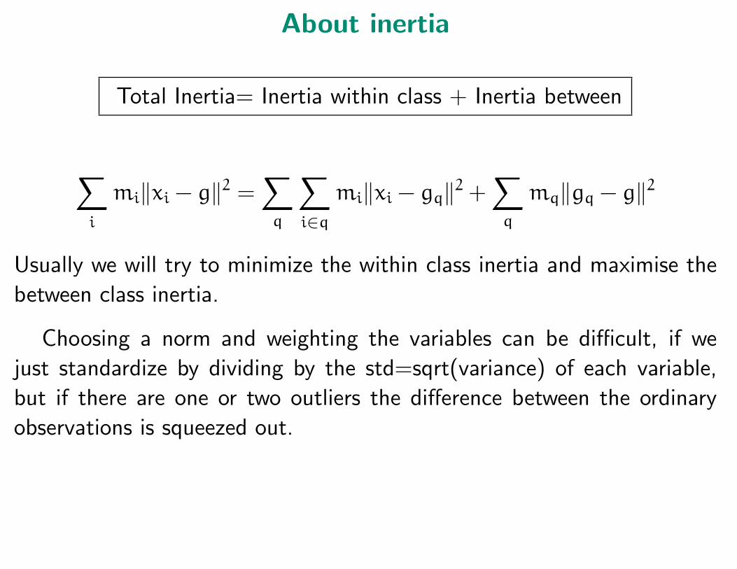
About inertia

Total Inertia= Inertia within class + Inertia between

∑i

mi‖xi − g‖2 =∑q

∑i∈q

mi‖xi − gq‖2 +∑q

mq‖gq − g‖2

Usually we will try to minimize the within class inertia and maximise the

between class inertia.

Choosing a norm and weighting the variables can be difficult, if we

just standardize by dividing by the std=sqrt(variance) of each variable,

but if there are one or two outliers the difference between the ordinary

observations is squeezed out.

Other renormalizations can be used:

• interquartile range.

• functions of the range.

• trimmed std.

Here is a summary of the essential choices implied in a hierarchical

clustering procedure:

Are the data tree-like?

One of the questions which sometimes is not addressed, and should

be, is the validity of choosing a hierarchical clustering procedure to begin

with.

For instance it is dangerous to build a tree, maximising some kind of

within inertia and then ask whether the inertia is significant as compared

to random clusters.

However for the non-biologist looking at the data a first question

comes to mind : Are trees the best way to represent the data? Sattah

and Tversky (1977) compare the tree representation to multidimensional

scaling.

One of the drawbacks the biologists have run into using trees is that

it has been difficult up to now to combine information from different

trees, for instance a tree built from DNA sequences and a tree built from

morphometric data ? Whereas combining multidimensional scaling maps

is possible along the same lines as the conjoint analysis methods.

Agglomerative Coefficient

agnes computes a coefficient, called Agglomerative Coefficient, which

measures the clustering structure of the data set. Agglomerative

coefficient is defined as follows:

-Let d(i) denote the dissimilarity of object i to the first cluster it is

merged with, divided by the dissimilarity of the merger in the last step of

the algorithm.

-The agglomerative coefficient (AC) is defined as the average of all

[1− d(i)]

Note that the agglomerative coefficient (AC) defined above can also be

defined as the average width (or the percentage filled) of the banner plot

described below.

Because AC grows with the number of objects, this measure should not

be used to compare clusters of data sets of very different sizes.

Non-hierarchical Clustering or Iterative Relocation

There are several intial choices to be made with these methods and

when the a priori knowledge is not available this can be a drawback. The

first is the number of clusters suspected. Each time the algorithm is run,

initial ‘seeds’ for each cluster have to be provided, for different starting

configurations the answers can be different.

The function kmeans is the one that can be used in R.

A more evolved method called Dynamical Clusters is also interesting

because it repeats the process many times and builds what is known as

‘strong forms’ which are groups of obervations that end up in the same

classes for most possible initial configurations.

Have to choose how many classes they will be prior to the analysis.

Can depend on the initial seeds, so we may need to repeat the analyses

over and over again.

Successful Perturbative Method for Non-hierarchicalClustering

Dynamical Clusters: Edwin Diday, 1970, 1972. [?]

• Repeated k-means with fixed class sizes.

– Choose a set of k nuclei (usually from the data).

– Partition the data as the nearest neighbors to each of the k points.

– For each partition define its centroid.

– Iterate the above 2 steps until convergence.

• This process gives a set of clusters.

• Organize these clusters according to sets of ‘strong forms” the ones

that were always together (or mostly) together.