Binary Encoding and Gene Rearrangement Analysis

Jijun Tang

Tianjin UniversityUniversity of South Carolina

jtang@cse.sc.edu(803) 777-8923

Outline

Backgrounds

Maximum Likelihood Methods for Phylogenetic Reconstruction

Maximum Likelihood Methods for Ancestral Genome Inferrence

Conclusions

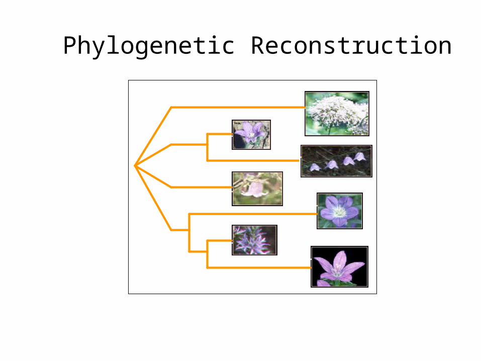
Phylogenetic Reconstruction

Data Type

Sequence Data

DNA/RNA/Protein Sequences

String on an alphabet of 4 or 20 characters

Gene-Order Data

Simple Rearrangements

Rearrangement Phylogeny

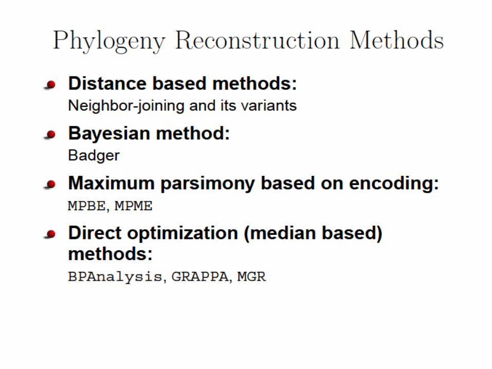
Median Problem

Goal: find M so that DAM+DBM+DCM is minimized

NP hard for most metric distances

Binary Encoding

Biased Model

Model of evolution:Duplications, insertions and deletions of syntenic blocksRearrangements: inversions, translocations, fusions, fissions

Binary sequences: 1(presence) vs. 0(absence)Adjacency: Pr (1 ->0) vs. Pr (0 -> 1)Gene content: Pr (1 -> 0) vs. Pr (0 -> 1)

Strong bias:Pr (1 ->0) >> Pr (0 ->1) for adjacencyLose an existing adjacency: Pr (1->0) 1/O(n)Gain a new adjacency: Pr (0 -> 1) 1/O(n2)

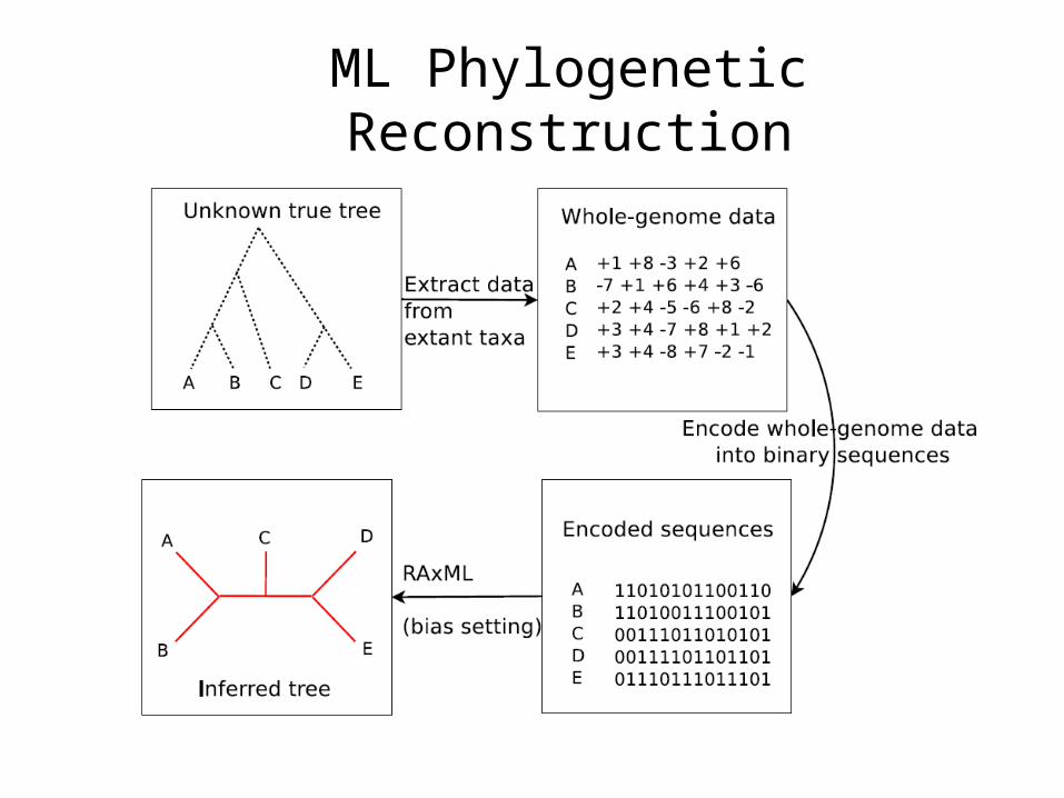
ML Phylogenetic Reconstruction

Simulated Results

Ancestral Inference

Step 1. Encoding gene orders into binary sequences.

Step 2. Setup the biased transition model.

Step 3. Arrange target ancestor to the root, and calculate the probabilities of character states for each character in the root.

Step 4. Building the adjacency graph and use a greedy heuristic to assemble adjacencies into valid gene order for the target ancestor.

Probabilities are calculated with a bottom-up recursive manner, so the target ancestor is placed to the root to prevent information loss.

Step 3 – Root Tree

Likelihood of a tree given sequence data at leaves can be computed (Felsenstein1981)

X Y ZW 1 1 00

01 01

01

X Y ZWPick one

tree

Pick one

site

Step 3 –Probabilities of Adjacencies

Posterior probabilities of character states (0 and 1) can be calculated according to Yang (Yang1995).

This is calculated by summing over all other ancestral states except root

8 histories8 histories 4 histories +4 histories +4 histories4 histories

Step 3 –Probabilities of Adjacencies

Independent adjacencies are assembled into valid gene order permutations by a greedy heuristic proposed by Jian Ma (Ma2007).

Sort the edges by weight.

Add the current heaviest edge to the path until a cycle is formed, then repeat the process until all vertices are traversed.

Remove the lightest edge in each cycle.

(1 -4 -3 5 2)(1 -4 -3 5 2)

Step 4 – Assemble Adjacencies

Transition model and reroot procedure are necessary

Simulation Result

PMAG was compared with InferCarsPro (Ma2011) and GRAPPA_DCJ(Xu2008)

Results-2

Tests on Large Scale Dataset

ML on Binary Encoding is more accurate and thousands of times faster than other methods

Binary encoding reduces the complexity and allows us to using existing methods for sequence data

Biased transition model and rerooting procedure are very useful

Future work:Extend PMAG to handle a more general model of evolution, including gene indel and duplication

Missing Adjacencies?

Conclusions

Thank You!