Master Thesis, Department of Geosciences

Binary filters developed to enhance and extract features and trends from 3D fault likelihood coherence data

Aina Juell Bugge

Binary filters developed to enhance and extract features and trends from 3D fault likelihood

coherence data

Aina Juell Bugge

Master Thesis in Geosciences

Discipline: Petroleum Geology and Petroleum Geophysics

Department of Geosciences

Faculty of Mathematics and Natural Sciences

University of Oslo Spring 2016

© Aina Juell Bugge, 2016 This work is published digitally through DUO – Digitale Utgivelser ved UiO http://www.duo.uio.no It is also catalogued in BIBSYS (http://www.bibsys.no/english) All rights reserved. No part of this publication may be reproduced or transmitted, in any form or by any means, without permission.

Abstract

This thesis presents a simple binary filter method for feature extraction and fault enhancement of

fault attribute data.

Fault attributes are commonly used in structural interpretive studies to detect faults. However, they

also tend to detect stratigraphic discontinuities and noise, and this provides a need to remove

unwanted features and to sort out important information. This has been the motivation behind this

thesis.

Structural geology, seismic interpretation and data processing have been combined to develop the

presented methodical approach. This approach involves converting the fault attribute data to

binary data, as well as assuming that each individual binary object has a set of properties that

represent fault properties and can be filtered. Each binary operation has been through an iterative

process of testing and evaluating different parameters for the most optimal use, and the procedure

has further evolved through this testing. All computational operations have been executed in

MATLAB r2014A and results have been evaluated subjectively in Petrel 2015.

Finally, development and application of seven binary filters is presented. They all in some way

measure properties of binary objects in two- and/or three-dimensions and they all, to some extent,

enhance or extract structural elements or trends.

The specific attribute data are fault likelihood coherence data derived from seismic data with a

semblance-based coherence algorithm. All completed filters are developed specifically for this fault

likelihood coherence data. However, it is assumed that other fault attribute data could be used after

some adaption.

The original seismic data is acquired in the southwest Barents Sea.

Preface

This paper presents a master thesis in Petroleum Geology and Petroleum Geophysics. It is written in collaboration with Lundin Norway AS and the Department of Geoscience at the University of Oslo. Dr. Jan Erik Lie, Prof. Dr. Jan Inge Faleide and Dr. Andreas K. Evensen have been supervising the work.

Lundin has provided the idea, data and necessary resources for this thesis and most work has been done in their offices in Oslo, Norway. The thesis work (ECTS 30) is the final part a of two-year master program (ECTS 120). The presented work will be further developed and implemented in a processing toolbox for Promax during the summer 2016 in collaboration with Lundin Norway AS.

Acknowledgements

First and foremost I would like to thank my supervisors; Dr. Jan Erik Lie (Lundin), Prof. Dr. Jan Inge Faleide (UiO) and Dr. Andreas K. Evensen (Lundin), for vital input and constructive feedback. All have provided valuable and necessary contributions to this work.

Lundin is acknowledged for providing topic, data and work place, and I would also like to thank all Lundin employees who have been available for questions during my stay. Especially, I would like to thank Steve Thomas for offering help and guidance with both the language and content in this thesis.

Further I would like to thank professors, lecturers and fellow students at the Department of Geoscience at the University of Oslo for all academic and social encounters these last five years. Finally, I want to thank my parents for taking an interest in my work and contributing with and guidance and input, especially related to language and phrasing.

Aina Juell Bugge, 2016.

TABLE OF CONTENTS

1. INTRODUCTION 1 1.1 Aim and outline 1 1.2 Faults: importance, characteristics and detectability 2 1.3 Structural framework in the acquisition area 5

2. COHERENCE IN FAULT DETECTION 9 2.1 Basics and applications of coherence 9 2.2 The mathematics behind coherence algorithms 12 3. DATA 17

4. A BINARY APPROACH TO FILTER COHERENCE DATA 21 4.1 Motivation and pitfalls 21 4.2 Workflow and introduction to binary operations 22

5. RESULTS FROM BINARY FILTERING 27 5.1 Preface to binary filtering results 27 5.2 Two-dimensional binary filtering 31 5.2.1 Area in 2D (F1) 32 5.2.2 Orientation in 2D (F2) 44 5.2.3 Clustering in 2D (F3) 48 5.2.4 Orientation and clustering in 2D (F4) 52 5.3 Introducing three-dimensional filtering 56 5.3.1 Area in 3D (F5) 57 5.3.2 Combined 2D and 3D area (F6) 59 5.3.3 Combined 2D orientation and 3D area (F7) 61 5.4 Summary of the results 64

6. DISCUSSION 67 6.1 Recommended strategy for use and potential improvements 67 6.2 Towards a quantitative evaluation of the results 68 6.3 Assessment and implementation of the procedure 70 6.4 Influence and importance of geology and data quality 72 7. CONCLUSIONS 75

8. REFERENCES 77

APPENDICES 81 Appendix I - 2D COHERENCE ANALYSIS IN MATLAB 82 Appendix II - UNUSED RESULTS 83 Appendix III - COMPLEMENTARY RESULTS 87 Appendix IV - FRACTALS AND FRACTAL DIMENSION 93

1

1. INTRODUCTION

1.1 Aim and outline

The objective for this thesis is to develop and exert new ways to filter fault likelihood coherence

data, as a filtering approach that enhance faults and fault trends could contribute to a better

structural understanding of an area. The idea is that when important information is accentuated and

noise is reduced, the structural geology can be better viewed and the following interpretation can be

more efficient.

Among numerous filter methods that exist, a binary approach was selected. This was selected after

investigation and testing of different filtering approaches, as it responded specifically well on the

provided attribute data. It is thought to be applicable on other reasonably imaged attribute data as

well, but it is however likely that a binary approach is best suited for high-quality data, as the data

dealt with in this thesis.

Specific aims for the thesis are to exploit this binary procedure and develop binary filters for the

fault likelihood coherence data. Each binary filter should in some way contribute to improve the

input data by enhancing or extracting specific structural features. This is done with relatively simple

and available tools and can, hopefully, in the future be used to aid structural seismic interpretation,

alone or combined with other existing methods.

The thesis consists of seven chapters, and the first introduces aim, outline and background

information considered necessary to interpret and evaluate results from filter operations. This

includes general perceptions of faults and of the structural settings in the acquisition area. Chapter 2

discusses coherence and how coherence algorithms can be used to detect discontinuities in seismic

reflection data. Chapter 3 describes provided data and chapter 4 briefly explains the most general

aspects of the binary procedure, and provides arguments for why filtering is necessary. Chapter 5

evaluates and discusses results from binary filtering and presents seven complete binary filters for

the fault attribute data. The discussion in chapter 6 aims to evaluate and discuss the filtering

approach and how to best implement it in seismic interpretation. Finally, conclusions are

summarized in chapter 7.

2

The appendices present derailments, complimentary elaborations and "dead ends" to the main flow

of the thesis work. This includes results that for some reason have not been used in filter

development, programming codes (MATLAB) and some necessary theory and explanatory

computations.

1.2 Faults: importance, characteristics and detectability

Faults and fractures are important in the petroleum industry as they affect both exploration and

exploitation of hydrocarbons. In some petroleum reservoirs faults can act as the seal that trap the

hydrocarbons. In others; faults can empty a reservoir by giving the fluids a pathway to escape. A

range of factors, not to be discussed here, controls how a fault allegedly affects the fluid flow in a

reservoir (Chester et al., 1993; Cornet et al., 2004; Braathen et al., 2009). Faults have also been

stated to in some cases improve reservoir quality by increasing porosity of the reservoir rock (Scott

and Nielsen, 1991; Aarre et al., 2012) and can cause hazards in well drilling (Aldred et al., 1999;

Aarre et al., 2012).

Generally, faults can be described as discontinuities in the earth’s interior and are results of

fracturing and displacement in rock volumes. Brittle responses to movements in the earth are

usually caused by plate tectonics; compressional-, extensional- or transversely related, and they

make up a vital part in understanding the structural geology in an area. Different stress regimes

cause different fault geometries. Normal faults are results of extension, reverse (and thrust) faults

result from compression and strike-slip faults occur in transverse regimes (figure 1.1).

Figure 1.1: Main fault geometries; normal-, reverse-, and strike-slip (illustration from: http://epicentral.net/faults/).

The fractured surface, usually referred to as the fault plane, is a three-dimensional feature with an

orientation determined by its strike and dip (figure 1.2). Strike (or azimuth, depending on the

notation) refers to the direction of the fault plane on a horizontal surface. Dip is the angle of the

3

fault plane relative to horizontal. Fault planes are often curved, so fault characteristics vary in

space.

Figure 1.2: Fault plane strike and dip (Brown, 2004).

Faults often occur in clusters, or zones, which are deformation areas in the crust weaker than the

surrounding rock (Chester et al., 1993). Fault zones consist of individual fault segments and/or fault

arrays, where fault arrays refer to more than one fault (Walsh and Watterson, 1989; Walsh et al.,

2003). Over time, fault growth can lead to interaction and overlapping of initially individual and

independent fault segments (Walsh et al., 2003).

There is no doubt that there is a need to understand the presence and characteristics of faults. The

problem lies with detecting them and interpreting them correctly. Reflection seismology is the most

common technique used to image the subsurface and thus to reveal faults. Seismic reflection data

are acquired as a receiver detects seismic signals that have been sent through and reflected on

internal layers in the earth (Ghosh, 2000; Gelius, 2004). Recordings are stored in two-dimensional

(2D) lines or three-dimensional (3D) cubes and display spatial changes in acoustic impedance;

seismic wave velocity and/or density (figure 1.3). These changes in the earth's interior can be

caused by sedimentary bedding, sequence boundaries, volcanic and salt intrusions, among some,

and are unanimously referred to as seismic reflectors (Gelius, 2004). Structural features such as

folds and faults will affect the seismic data and can bend or disrupt the continuity of these seismic

reflectors.

4

Figure 1.3: Two-dimensional seismic reflection data (data: Norsk Hydro AS in Brown, 2004).

In traditional fault interpretation, faults are detected by their tendency to truncate seismic reflectors

(figure 1.4). The faults can be interpreted manually with, or without, the help of an auto tracking

device. However, traditional fault interpretation tends to be biased as it is highly dependent on the

interpreter and the auto tracking device of the interpretive software. Manual geological

interpretation of seismic data also adds time between exploration and production and time-reduction

is generally economically beneficial (Randen et al., 2001).

Figure 1.4: Truncated seismic reflectors indicate presence of a fault (Data: Lundin Norway AS).

Not all faults are easy to see in seismic. Known and common difficulties are associated with

terminations of low amplitude events and fault planes oriented parallel to bedding. These obstacles

are often referred to as subtle faults and invisible faults, due to their low detectability (Aarre et al.,

2012). When a fault plane runs parallel or close to parallel to bedding plane, the fault will

consequently run parallel to the seismic reflector and not give a distinct reflector termination

(Brown, 2004; Aarre et al., 2012).

In seismic, faults are usually categorized as either planar or listric. Listric faults are curved and

flatten out with depth, which affect the seismic detectability as the terminated reflector will become

less and less visible. If the fault flattens out too much the fault itself becomes a reflector. Faults tend

5

to appear more listric in TWT (two-way time) on seismic sections than they really are in depth. This

occurs as the seismic velocity increases with depth (Turner and Holdsworth, 2002). As the fault

plane is a three-dimensional feature, two-dimensional seismic data will portray only a sliced view

of the fault plane, most likely with misleading fault characteristics. Only three-dimensional seismic

data can measure three-dimensional characteristics.

1.3 Structural framework in the acquisition area

The seismic data handled in this thesis is acquired near the Loppa High in the southwestern part of

the Barents Sea (figure1.5); an epicontinental sea located north of Norway (Gabrielsen et al., 1992;

Gudlaugsson et al., 1998). A basic understanding of the main structural trends and the timing of

responsible events in the study area is considered a prerequisite for the rest of the thesis. Any new

or own contributions to interpret the structural geology will however not be presented.

Figure 1.5: Location and main structural elements of the Barents Sea with highlighted acquisition area (based on NPD

fact maps, edited for own use).

The 300 km wide southwestern Barents Sea rift zone is thought to have been formed mainly during

the mid Carboniferous (Breivik et al., 1995; Gudlaugsson et al., 1998). A complex structural

evolution and extensive crustal thinning have led to developments of basins and highs, such as the

Loppa High; a sedimentary high surrounded by the Hammerfest Basin, the Tromsø Basin, the

Bjørnøya Basin and the Bjarmeland Platform (Gabrielsen et al., 1990; Gabrielsen et al,. 1992;

Breivik et al., 1998).

6

It is a general perception that a compressional tectonic event is responsible (at least to some extent)

for the dominant northeastern structural trend in the western Barents Sea today (Sturt et al., 1975;

Gabrielsen et al., 1990; Gudlaugsson et al., 1998; Ritzmann and Faleide, 2007). This compressional

event had two phases, an early phase in late Cambrian and a main phase in late Silurian-early

Devonian, and led to the formation of a major orogeny; the Caledonian mountain range (Ritzmann

and Faleide., 2007).

More detailed, the major structural trends in the SW Barents Sea can be subdivided into (Gabrielsen

et al., 1990):

1) ENE-WSW to NE-SW

2) NNE-SSW

3) WNW-ESE (more locally)

The Caledonian Orogeny established a fracture system; a zone of weakness in the basement rock

that influenced the following tectonic phases in the Barents Sea (Gabrielsen et al., 1990; Gabrielsen

et al., 1992). New stress-regimes, even those with different orientation and polarity, adapted to this

established trend and re-activated pre-existing faults (Cooper et al., 1989; Gabrielsen et al., 1992).

Post-Caledonian tectonics was dominated by crustal extension, which contributed to a series of

rifting, subsidence, tilting, uplift, erosion and inversion events (Gabrielsen et al., 1992; Faleide et

al., 1993; Gudlaugsson et al., 1998). Inversion structures; inside out turning of basins, are thought to

be a result of changes in stress regimes (Williams et al., 1989, Gabrielsen et al., 1992).

Comprehensive fault systems and reactivations have made it difficult to determine the number,

timing and relative importance of the different tectonic phases (Gabrielsen et al,. 1992;

Gudlaugsson et al., 1998). They have also varied locally in the Barents Sea, and the northeartern

part became more tectonically stable before the southwestern part (Gabrielsen et al., 1990;

Gudlaugsson et al., 1998).

Today, the western Barents Sea subsurface consists of Caledonian metamorphic basement rocks

covered by sedimentary packages ranging in age from Late Palaeozoic to present (Gabrielsen et al.,

1992; Faleide et al., 1993; Gudlaugsson et al., 1998; Ritzmann and Faleide., 2007).

7

Figure 1.6 illustrates the structural styles of the study area as well as listing the primary structural

events which affected the study area (Glørstad-Clark et al., 2011). Sedimentary successions from

Devonian to Triassic are represented on Loppa High in addition to Quaternary glacial sediments

(Gabrielsen et al., 1990). The Polheim Sub-platform is less affected by erosion and has preserved

more post-Triassic deposits. Thick, deltaic, early Mesozoic packages are results of a strong

sedimentary influx from the east in Triassic time (Gabrielsen et al., 1990; Glørstad-Clark et al.,

2010, 2011).

The Ringvassøy-Loppa Fault Complex was active at least four times since Devonian, and the

structural high present today is an assumed result of extensional tectonic events in Jurassic-early

Cretaceous and early Cretaceous-Tertiary (Gabrielsen et al,. 1990; Faleide et al., 1993). Its majority

of faults are Jurassic/early Cretaceous extensional faults (normal faults) striking north, and some

probably involved basement faulting (Gabrielsen, 1984; Gabrielsen et al,. 1993; Faleide et al., 1993;

Ritzmann and Faleide, 2007).

8

a)

b) Figure 1.6: a) Interpreted faults and sedimentary packages near the Loppa High and the Polheim Sub-platform, edited

to highlight acquisition area. b) Corresponding event chart. Both from: Glørstad-Clark et al., 2011.

9

2. COHERENCE IN FAULT DETECTION

2.1 Basics and application of coherence

A coherence analysis is one of many techniques used to detect and classify discontinuities in the

earth’s interior on seismic data. Simply put, the analysis employs a coherence algorithm to obtain

measurements of multi-trace relationships based on how coherent (similar) neighboring signals are

(Bahorich and Farmer, 1995). This is illustrated in figure 2.1.

Figure 2.1: Sketched basics of a coherence analysis. 𝜏 denotes a time shift.

Different coherence algorithms have been proposed over the last decades. They operate in two or

three dimensions and calculate coherence coefficients as a function of waveform likeness for a

given number of neighboring seismic traces. Today, cross-correlation, semblance and eigenstructure

are the most common coherence algorithms (Bahorich and Farmer, 1995; Marfurt et al., 1998;

Gerztenkorn and Marfurt, 1999; Chopra, 2002; Hale, 2012, 2013)

The coherence coefficients are derived with a chosen algorithm that calculates the similarity of

neighboring seismic time signals, i.e. seismic traces, within a sliding analysis window (figure 2.2).

10

Figure 2.2: Sketched coherence analysis of seismic traces. High coherence is measured along the seismic reflector (red

line). Termination indicates low coherence and a potential discontinuity.

When derived from seismic data, high coherence coefficients indicate high trace similarity and

ideally represent continuous seismic reflectors. Conversely, lower coherence coefficients represent

discontinuous or terminated seismic reflectors (figure 2.3). Hence, the coherence analysis

potentially reveals faults as low coherence regions numerically separated in space from the

surrounding data (Bahorich and Farmer, 1995).

Figure 2.3: From left: 1) Seismic line, 2) seismic line and detected discontinuities, 3) only detected discontinuities.

Detected discontinuities are obtained with a coherence algorithm (Data: Lundin Norway AS).

Coherence is considered a seismic attribute (a post-stack, window–based attribute) and generates a

new dataset from the existing. It is however, a derivative of basic information; time, and displays

data in a new way (Brown, 2004).

Figure 2.4 illustrates how a simple two-dimensional coherence analysis calculates coherence

coefficients (B) from seismic data (A). The analysis is executed in MATLAB and procedure can be

found in Appendix I. Terminated seismic reflectors observed in the seismic data correspond to areas

11

of low detected coherence. This shows that low coherence regions can be interpreted as

discontinuities and ideally reveal faults.

Figure 2.4: 2D seismic line (A) and corresponding coherence line (B). This specific coherence analysis executed in

MATLAB and explained in Appendix I.

Calculated coherence values for all points in a seismic volume result in a coherence cube; a three-

dimensional cube of coherence coefficients. As the coherence cube reveals faults and other

discontinuities with minimum interpretational bias, coherence analysis is cost-efficient and time

saving compared to manual fault interpretation in seismic data (Skirius et al., 1999).

Figure 2.5 displays a seismic time slice and corresponding time slice extracted from the coherence

cube. Complex fault geometries with major and minor faults, and even faults that run parallel to

strike, become visible on the coherence time slice. Where fault visibility on regular seismic data

depends on their orientation relative to structural strike, all discontinuities will be equally detectable

in coherence data (Bahorich and Farmer, 1995; Brown, 2004).

12

Figure 2.5: a) Seismic time slice, b) coherence time slice (Data: Lundin Norway AS).

Another application of coherence is derivation of coherence coefficients from interpreted seismic

horizons. This will however not exclude interpretational bias and is more common in geological

studies used to detect lithological contrasts caused by channels, point bars, canyons, slumps, tidal

drainage patterns etc. (Marfurt et al., 1998; Bahorich and Farmer, 1995).

2.2 The mathematics behind coherence algorithms

The first coherence algorithm for geophysical appliances was cross-correlation-based and

introduced by Bahorich and Farmer in 1995.

Cross-correlation, C, is in general described as a measure of similarity between two signals and can

mathematically be written in the discrete domain as:

𝐶 = 𝑠1(𝑡) ∗ 𝑠2(𝑡 + 𝜏),

where * represents the cross-correlation operation that sums together all multiplications of the

amplitude of one signal (s1) with the time shifted amplitude of a neighboring signal (s2). 𝑡 is time

13

and the time shift, or lag, (𝜏) represents how much one signal must be moved in time to best match

the other (figure 2.6). For best possible match, cross-correlation is at its maximum and the peaks of

the two signals will be aligned.

Figure 2.6: Sketch illustrates a time shift (𝜏) between two seismic signals, s1 and s2.

In signal processing it is common to use normalized cross correlation (Lines and Newrick, 2004).

This will produce correlation coefficients between zero and one. The normalized cross correlation

takes use of the energy of the two signals and can be written as:

𝐶 = 𝑠1(𝑡) ∗ 𝑠2(𝑡 + 𝜏)

�𝐸𝑠1𝐸𝑠2.

The energy, E, of a discrete signal 𝑥(𝑡) is generally defined as ∑ |𝑥(𝑡)|2𝑑𝑡∞−∞ , and the energy of s1

and s2 can be written as ∑ 𝑠12(𝑡𝑖)𝑖 and ∑ 𝑠22(𝑡𝑗)𝑗 respectively. Thus, the normalized cross

correlation equation can be extended and written as (Lines and Newrick, 2004):

𝐶 =∑ 𝑠1(𝑡𝑖)𝑠2(𝑡𝑗 + 𝜏)𝑖

�∑ 𝑠12(𝑡𝑖)𝑖 ∑ 𝑠22(𝑡𝑗)𝑗 �1/2.

Exact shape of s1 and s2 at an alignment t (even though the amplitudes can vary) will give C=1.

This will, if measured along a seismic reflector, indicate that it is perfectly continuous.

The cross-correlation algorithm (and any other coherence algorithm) derives coherence coefficients

within a spatial analysis window. The window is centered on an analysis point and calculates

coherence within the window before the window is moved in space. Seismic signals are often

shifted in time due to non-horizontal seismic reflectors.

ANALYSIS WINDOW

14

It is therefore crucial that the analysis window has the same dip and azimuth as the local seismic

horizon and knowledge of the structural dip is essential for a successful coherence analysis. By

selecting a dip and azimuth at the analysis point that gives the largest positive normalized cross-

correlation value, the dip and azimuth of the analysis window will approximately match the dip and

azimuth of the seismic reflector (figure 2.7) and hence, local dip is accommodated for (Chopra and

Marfurt, 2007). Cross-correlation can thus also be used as a technique for automatic dip-extraction

(Hale, 2012, 2013).

Figure 2.7: Sketch illustrates a time shift that can be explained by dipping seismic reflectors. The analysis window

adapts to this dip when calculating coherence.

For a 3D measure of coherence, the signal at the analysis point is compared to its two closest

neighbors in inline and crossline direction (figure 2.8). For this, a minimum of three traces are

required, although more than three can reduce occurrence of granular noise and increase the data

quality (Chopra and Marfurt, 2007). The three-trace-cross-correlation algorithm is sensitive to

waveform and noise but not to amplitude changes (Chopra and Marfurt, 2007). It lacks robustness,

but has high computationally effectiveness as only three traces are used (Gersztenkorn and Marfurt,

1999).

15

Figure 2.8: Sketch of a three-trace-analysis window (3D coherence analysis). S1 is at the analysis point and S2 and S3

are closest neighbors in inline and crossline direction.

Mathematically, a three-dimensional coherence coefficient is obtained by combining the calculated

maximum cross-correlation in both inline and crossline direction (Marfurt et al., 1998):

𝐶𝑥𝑥 = �� 𝐶𝑥(𝑡, 𝜏(𝑙), 𝑥𝑖, 𝑦𝑖)𝜏(𝑙) 𝑚𝑚𝑥 �� 𝐶𝑥(𝑡, 𝜏(𝑚), 𝑥𝑖 ,𝑦𝑖)𝜏(𝑚)

𝑚𝑚𝑥 � .

Here 𝜏(𝑙) and 𝜏(𝑚) are the respective lags for maximum cross-correlation in two directions (𝐶𝑥 and

𝐶𝑥) and 𝑡 is time between traces at positions 𝑥𝑖 and 𝑦𝑖. 𝐶𝑥𝑥 is then the three-dimensional estimate of

coherency. Only by combining the maximum cross-correlation values for inline and crossline

correlation coefficients, the window dip will be (approximately) equal to the structural dip (Chopra

and Marfurt, 2007).

There are many ways of measuring similarity of signals, and coherence algorithms have been

upgraded over time as technology has evolved. Some more advanced coherence algorithms are the

multitrace semblance-based algorithm (Marfurt et al., 1998), the eigenstructure-based algorithm

(Gersztenkorn and Marfurt, 1999), the higher-order-statistics based algorithm (Lu et al., 2005) and

the super trace eigenstructure-based algorithm (Li et al., 2006).

Semblance is a measurement of trace relationship similar to cross-correlation that estimates

coherency using a semblance analysis over an arbitrary number of traces. Whereas cross

correlation-based coherency is derived from the sum of products of seismic amplitudes, semblance

divides the energy of the sum of trace amplitudes by the sum of energy of the traces (Lines and

16

Newrick, 2004). In contrary to the simplest cross-correlation algorithm which only relied on three

neighbor traces, the semblance algorithm uses five-, nine-, or more neighboring traces (Chopra and

Marfurt, 2007). A 5-trace analysis window is illustrated in figure 2.9.

Figure 2.9: Sketch of a 5-trace analysis window.

The semblance-based algorithm is more stable when dealing with noisy data than the cross-

correlation-based (Gersztenkorn and Marfurt, 1999; Cohen et al., 2006). The analysis window

centered on the analysis point must still have the same dip as the target horizon, either set by user-

definition or through calculations (Chopra and Marfurt, 2007; Wang and AlRegib, 2014). The

analysis point then defines a local planar event at time t, with apparent dips in two directions

(Marfurt et al., 1998). An analytic representation of the original signal in the same domain gives a

complex-valued function and semblance is then calculated of the analytic trace (Marfurt et al.,

1998).

Eigenstructure-based coherence computations were introduced by Gersztenkorn and Marfurt in

1999. Of the three discussed algorithms, eigenstructure provides the most robust results

(Gersztenkorn and Marfurt, 1999). The algorithm is based on the eigenstructure of a covariance

matrix. It is possible to assume zero dip and azimuth, but this will give structural artifacts. By first

calculating and applying dip and azimuth one gets artifacts-free results (Chopra and Marfurt, 2007).

Both semblance and eigenstructure suffer from sensitivity of waveform and lateral amplitude

changes (Chopra and Marfurt, 2007).

17

3. DATA

Lundin Norway AS has provided three-dimensional seismic data and corresponding fault likelihood

coherence data of high quality for this thesis (figures 3.1 and 3.2).

The provided seismic volume (LN15M03) is a merge of several seismic datasets acquired near the

Loppa High in the southwest Barents Sea. Inline range is 31400-28300 and crossline range is

26814-24838, both with increment 2 and 25 meter intervals. The volume extends over 949 km2

laterally and 3 seconds vertically, with a sample rate of 4 ms (751 samples per trace). Inlines are

directed N-S and crosslines are directed E-W.

The fault likelihood coherence data is derived from the original seismic data. Coherence values for

each point in the dataset have first been calculated with a semblance-based coherence algorithm.

Further, fault likelihood has been estimated from the semblance values. Fault likelihood is defined

as 1 – ss, where s is the semblance value. This represents the likelihood of a point being part of a

fault surface (Cohen et al., 2006; Wang and AlRegib, 2014). All assumed fault surfaces have been

through a thinning operation for visual enhancement.

The size of the attribute volume is the same as the seismic volume except for a vertical reduction to

2,5 seconds and all points in the fault likelihood coherence data are given as fault likelihood

amplitudes ranging from zero to one. A more detailed description of the specific attribute algorithm

will not be presented here as it is not available in the public domain.

Figure 3.1 display seismic lines and time slice from the provided seismic data, and figure 3.2

display the corresponding fault likelihood coherence data.

18

Figure 3.1: Seismic lines and time slice from the provided data.

19

Figure 3.2: Coherence lines and time slice, derived from original seismic in figure 3.1.

20

Time slices display fault trends best as distribution and orientations can be studied on them.

Orientation measured on a time slice will represent the strike (or azimuth) of the measured feature.

Inlines and crosslines display other fault characteristics such as apparent dip.

The main NE structural trend in the western Barents Sea (e.g. Gabrielsen et al., 1990; Faleide et al.,

1993; Gudlaugsson et al., 1998; Ritzmann and Faleide, 2007) can be observed in the provided data.

However, a more or less directly northern trend is just as prominent (figure 3.3). The northern trend

varies slightly between NNE and NNW but is mainly directed N-S and is parallel to the western

fault of the paleohigh referred to as the Selis Ridge (Glørstad-Clark et al., 2011). This paleohigh is

displayed in figure 1.6. Most observed faults in the data are normal faults due to the extensional

history in the area.

Figure 3.3: Observed main structural trends drawn on fault likelihood coherence time slice (1,5 s).

21

4. A BINARY APPROACH TO FILTER COHERENCE DATA

4.1 Motivation and pitfalls

Although the coherence analysis provides a technique for detecting faults with less bias than

conventional fault interpretation, there are still issues that should be addressed. Stratigraphic

discontinuities comprise potential pitfalls as coherence algorithms fail to differentiate between

different types of discontinuities (Bahorich and Farmer, 1995). Other problems are typically related

to noise.

Noise is a subjective term and can be defined as "unwanted energy" in seismic recordings (Scales

and Snieder, 1998) or as all that disturbs the signal from a reflector (Hesthammer and Fossen,

1997). It originates from numerous sources and can be recordings related to the environment; such

as waves in the ocean, to seismic acquisition; such as vibrations from the acquisition vehicle, or

different types of multiples, seismic artifacts and effects from processing (Scales and Snieder,

1998).

In fault likelihood coherence data, noise can be defined as all recordings that do not comprise

structural discontinuities and that are not important for the structural geology in the area of interest

(figure 4.1).

Figure 4.1: Seismic data (left) and coherence data (right). Stated observations are based on subjective interpretations.

22

All seismic data, and thus all attribute data, will be affected by noise, often categorized as

systematic or random noise (Hesthammer and Fossen, 1997). In structural studies, systematic noise

typically comprises the largest pitfall as it potentially has a linear or curved-linear appearance

(Hesthammer and Fossen, 1997) and can be misinterpreted as a structural feature, both by people

and algorithms.

Automatic or semi-automatic methods for noise reduction and faults enhancement have been

introduced the last few decades. Gibson et al. proposed in 2005 a workflow that extracts faults

based on the merge of likely fault points into larger three-dimensional surfaces. Cohen et al. (2006)

presented a multi-directional filter with a threshold to enhance contrasts of fault likelihood points,

and Hale (2013) introduced an automatic three-step process of computing fault likelihood data

together with dip and strike measurements, extracting fault surfaces and finally estimating fault

throws. In 2014, Wang and AlRegib proposed a fault feature detection algorithm based on Hough's

transform that converts fault likelihood points to parametric representations of lines to be classified

as either fault features or false features. Another commonly accepted fault extraction method is "Ant

tracking" (Pedersen, 1999; Pedersen et al., 2002, 2003). This technique codes virtual ants to track

discontinuities in fault attribute data and then further extract these tracked faults (Pedersen, 1999).

Here, a procedure that targets all detected discontinuities as binary objects is presented. Although

the specific input data is fault likelihood data derived with a semblance-based coherence algorithm,

the filter method is thought to be applicable on other fault attribute data as well.

The binary procedure was chosen specifically for the provided data. This was not a pre-determined

method for the thesis, but was selected based on its ability to be applied with relatively simple tools

and that it early on showed promising results. Other procedures were considered, but for various

reasons they were abandoned. The high quality of the fault likelihood data is thought to be a

controlling factor here and it is likely that for noisier input data, other methods could be preferred.

4.2 Workflow and introduction to binary operations

The filtering procedure deploys binary operations, and this requires that the input is first converted

to binary data. Binary data is expressed by only two symbols, such as zeroes (0) and ones (1), and

23

stored in a binary matrix, also referred to in literature as logical-, integer-, relation- or Boolean

matrix, with one or more matrix dimensions (O’Neil and O’Neil, 1973). Here, the binary

conversion involves transforming all fault likelihood amplitudes larger than zero to ones (figure

4.2).

Figure 4.2: Fault likelihood points before and after binary conversion.

With this, the variation in fault likelihood amplitudes is removed and ones will represent any

likelihood of a present discontinuity. Alternatively this conversion could have been done with

another preferred threshold.

Connected ones now represent binary objects. These binary objects can ideally be thought of as

individual discontinuities and can be subjected to binary operations that change, extract or remove

specific properties or trends. Issues occur if two discontinuities interfere and are detected as one

object. This will be addressed when encountered.

Different operations are extensively tested and evaluated from a mainly interpretive and subjective

point of view as most settings and parameters are decided from what produces best results.

Successful operations are further exploited and used to develop complete binary filters for the fault

likelihood cube.

Binary operations are applied in an iterative process where it is repeated with new settings and

parameters until either discarded or implemented in a binary filter. Figure 4.3 shows a sketch of the

main steps in the workflow.

24

Figure 4.3: Sketch of workflow chart for the presented method.

All computational operations are carried out in MATLAB R2014a. Petrel 2015 is used to evaluate

the results from the different binary operations. Figure 4.4 illustrates data format and software used

in the main steps of the workflow. Other computer languages and other interpretational software

could alternatively be used.

Figure 4.4: Sketch illustrates data format and software used in different steps of the workflow.

Properties studied in this thesis are size, distance to neighbor objects, orientation, axis lengths and

geometries/shapes. Some central object properties are illustrated in figure 4.5 and 4.6.

Object size can be defined differently, such as with a calculated area, given as the number of

connecting ones. Another measure of object size is the length of the objects major axis. Major axis

is defined as the longest detectable axis measured in number of pixels. As the major axis is the

longest axis, the minor axis is consequently the shortest. For three-dimensional objects a third axis

can also be measured. Axis orientation and lengths can give an approximate idea of an objects

25

shape and extent. Orientation, or direction, is measured as degrees between the x-axis and the major

axis. This varies from -90° to 90°.

Figure 4.5: Sketch illustrates area, major axis and orientation of a binary object.

Distance is typically measured as the number of pixels between two binary objects. It can be

derived between all points of the two objects, or derived as a scalar such as; minimum distance,

maximum distance or average distance.

Information of the binary objects axis lengths can be used to study object shapes. Other properties,

such as extreme points, center points and eccentricity can also be used to indicate object shape. The

center point refers to the location of the point in the middle of the binary object whereas extreme

points can be thought of as the location of the corners of the binary objects (Márquez et al., 2011).

Figure 4.6: Sketch illustrates center point of a binary object, extreme points of a binary object and minimum distance

between two binary objects and

The eccentricity can be thought of as an indication of object shape as it in mathematics defines how

much an object shape differs from a circle. Eccentricity can be derived from the ratio of the distance

between the foci (center point) of an ellipse and its major axis length (Salas, 2004). In 2D, 0 denotes

a circle and 1, a line segment (figure 4.7).

26

Figure 4.7: Sketch illustrates different values of eccentricity.

Binary operations are tested on arbitrary small volumes in 3D and/or arbitrary inlines, crosslines or

time slices in 2D (figure 4.8).

Figure 4.8: Illustration of a 3D cube, inline, crossline and time slice and their respective axes.

It must be emphasized that one pixel does not represent the same geographical distance in all

directions. Just as seismic data, it has time (s) on the vertical axis and length (m) on the two

horizontal axes. This means that all areas, lengths, directions and other binary measurements must

be treated with care if they are to be projected to geographical measurements.

For the specific data in this thesis a distance of one pixel on a time slice (x- and y- directions)

corresponds to 25 meters, while the same pixel distance down an inline or crossline (z-direction)

corresponds to 4 milliseconds (figure 4.9). The seismic velocity in the given area at depths of 1-1,5

seconds is estimated to be ~3,2 km/s (J. I. Faleide, 2016, pers. comm. April 15.). One pixel in z-

direction is thus ~12,8 m.

Figure 4.9: Sketch illustrates pixel size for the binary fault likelihood data in this thesis.

27

5. RESULTS FROM BINARY FILTERING

5.1 Preface to binary filtering results

This chapter presents development of, and results from, seven binary filters to be used for fault

likelihood data (table 5.1). The main focus has been two-dimensional binary filtering. A sole three-

dimensional procedure is also briefly introduced, before a combined 2D/3D procedure is pursued.

Two-dimensional binary operations benefit from being relatively easy to apply and comprehend.

However, only three-dimensional operations can obtain three-dimensional property measurements,

and these will likely be closer to true fault properties. A summary of the presented binary filters is

found at the end of this chapter.

Table 5.1: A presentation of binary filters with a short description.

FILTER Dimension Short description

F1 2D Target noise and insignificant discontinuities in different directions

F2 2D Separate fault orientations

F3 2D Aims to extract fault zones based on clustering

F4 2D Aims to extract fault zones based on orientation and clustering

F5 3D Targets major faults in 3D

F6 2D/3D Targets major faults in 3D after first filtering area in 2D

F7 2D/3D Targets major faults in 3D after separating fault into orientation groups in 2D

The following unused and complimentary results are included in the Appendix II and III:

- Results from targeting object geometry

- A table presenting the default settings and parameters for the filters (Table A1)

- Codes (MATLAB scripts) for all completed filters (F1-F7)

Unused results are results from binary operations that were not used in filter developments, either

due to unsuccessful results or due to scope limitations. This involves mainly operations that initially

were meant to target fault geometries (or shapes) and morphological alterations; ways of changing

28

object shape. These operations are presented and discussed in Appendix II. The MATLAB codes

and a table of recommended parameters are included as complementary results in Appendix III.

Properties that have proven useful and thus have been exploited in different ways to develop filters

are area, distances and orientation. The final binary filters are applied on small sub-volumes for

computational efficiency. The sub-volume is extracted from an approximate center of the initially

provided data volume (figure 5.1).

Figure 5.1: Relative size of extracted sub volume compared to the provided seismic volume.

Sub-volumes or sub-cubes are also used for illustration purposes. Figure 5.2 displays the seismic

sub-cube, the fault likelihood sub-cube and the binary fault likelihood sub-cube. Time slices from

the center of the respective cubes are also shown. The binary sub-cube and its center time slice are

used throughout the thesis to present the results from the final filters, unless another or an additional

view is more explanatory. Steps, issues or pitfalls are shown on arbitrary lines or slices that are

selected based on ability to illustrate the specific phenomenon.

The sub-cube is 25 km2 in lateral extent and its vertical thickness is 0,5 seconds (124 samples).

After conversion, the binary sub-cube consists of 201x201x124 binary pixels.

29

Figure 5.2: Time slices and sub-cubes from seismic-, fault likelihood- and binary fault likelihood data.

30

The sub-cube is relatively shallow and covers Triassic sedimentary packages faulted by (mainly)

Late Jurassic-Early Cretaceous normal faults. It represents all major structural trends (figure 5.3)

and its structural framework is considered representative for the entire volume.

Seismic resolution defines the limits of how much detail that can be observed in the seismic and it

will decrease with vertical depth as the seismic wavelength increases (Sheriff, 1985, 1996). As the

sub-volume is shallow; 1-1,5 seconds, the seismic is of relatively high quality. It is thus assumed

that the sub-cube has higher seismic quality; better displayed details and less interference than

deeper sections in the same seismic volume. However, as the entire volume also is relatively

shallow (0-3 seconds) it has an overall good quality, but vertical and horizontal differences can be

expected.

Figure 5.3: Major observed fault trends illustrated on a time slice from the fault likelihood sub-cube.

31

5.2 Two-dimensional binary filtering

Development and application of four two-dimensional binary filters; F1, F2, F3 and F4, is presented

in this sub-chapter. Generally, two-dimensional filters suffer from un-true object properties and

direction-dependent results. Two-dimensional operations target object properties on time slices,

inlines or crosslines so selected direction must be specified. The same binary operation will provide

different outcome for the three different directions and can even target different properties as the

axis operate with different scales and units. There is no preferred direction for all situations, and

input, wanted output and the type of operation should be considered upon selection. Thus, viewing

a fault from the three different orthogonal directions gives three different visualizations of the fault

due to how the slice or line intersects the discontinuity (figure 5.4).

TIME SLICE CROSSLINE INLINE

Figure 5.4: A binary object (assumed fault) displayed from three directions).

Inlines or crosslines with orientation similar to orientation of a fault plane tends to view this fault as

a wide, odd feature. This is especially true for steep dipping faults. A line oriented approximately

90 degrees to the fault plane typically detects a sharper discontinuity more typical of thought fault

plane geometry. The concept is attempted to be explained with the sketch presented in figure 5.5.

Figure 5.5: Sketch illustrates how 2D detections of 3D features can be misleading. Left: steep-dipping fault oriented

similarly to line. Right) fault plane oriented with a high angle to the line (near orthogonal).

32

Time slices portray a horizontal view of the fault plane at a specific depth in time and are less

affected by how the seismic lines intersect the fault plane. However as 3D fault planes vary their

extent in space and usually curve, the viewpoint is still crucial on time slices (figure 5.6).

Figure 5.6: Sketch illustrates how different time slices detects the same fault differently.

How a discontinuity is viewed in 2D is a combined effect of mainly how the lines are oriented, and

on the structural geology; fault orientation, size and characteristics. Additionally, data quality

determines if a lot of noise is wrongfully included and resolution controls detectability; how small

discontinuities that are detected, and how close they can be without appearing as one.

The final 2D-filters should be applicable to a three-dimensional volume. This is done by filtering

separatly on all timesclices, all inlines or all crosslines in the volume and then merge these back

into a signle cube (figure 5.7).

Figure 5.7:Sketch illustrates how3D data can be filtered in 2D by filtering either all time slices or all lines in the cube

(in one direction).

5.2.1 Area in 2D (F1)

Filter F1 addresses binary object size. The idea is that by removing all objects smaller than a

specified size, noise and smaller discontinuities are removed, and major faults are accentuated. This

can ideally improve the understanding of the structural framework.

33

Figure 5.8 illustrate examples of objects that, based on a subjective interpretation, could be

beneficial to remove.

Figure 5.8: Arbitrary time slice from unfiltered cube with highlighted areas showing examples of assumed unimportant

objects for the structural framework (targets for filtering).

Different ways of defining object size could be used in F1. A comparison of area and major axis

length is included in Appendix II. The comparison indicated that both seemed useful for the

purpose of removing minor objects. However, area was chosen as the default criteria measurement

of size for F1.

PROCEDURE OF F1:

1) Detect all individual binary objects

2) Measure area of each object

3) Remove all smaller than a user-defined area

The procedure of F1 is tested on one time slice, one crossline and one inline and the results are

portrayed in figure 5.9. All settings and parameters are equal for the three recursions. Minimum

area criterion is set by the user. It is here set to 30 pixels. All objects with areas less than this is

removed. This choice of parameter is further discussed later.

34

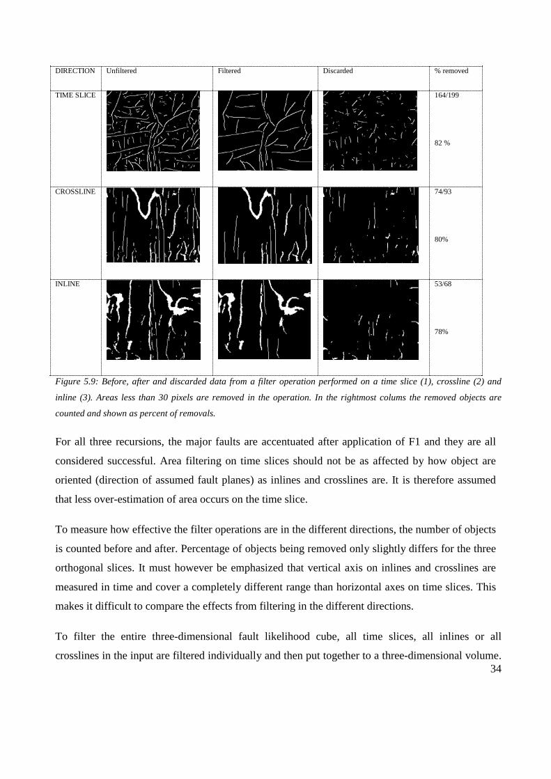
DIRECTION Unfiltered Filtered Discarded % removed

TIME SLICE

164/199

82 %

CROSSLINE

74/93

80%

INLINE

53/68

78%

Figure 5.9: Before, after and discarded data from a filter operation performed on a time slice (1), crossline (2) and

inline (3). Areas less than 30 pixels are removed in the operation. In the rightmost colums the removed objects are

counted and shown as percent of removals.

For all three recursions, the major faults are accentuated after application of F1 and they are all

considered successful. Area filtering on time slices should not be as affected by how object are

oriented (direction of assumed fault planes) as inlines and crosslines are. It is therefore assumed

that less over-estimation of area occurs on the time slice.

To measure how effective the filter operations are in the different directions, the number of objects

is counted before and after. Percentage of objects being removed only slightly differs for the three

orthogonal slices. It must however be emphasized that vertical axis on inlines and crosslines are

measured in time and cover a completely different range than horizontal axes on time slices. This

makes it difficult to compare the effects from filtering in the different directions.

To filter the entire three-dimensional fault likelihood cube, all time slices, all inlines or all

crosslines in the input are filtered individually and then put together to a three-dimensional volume.

35

All three filter directions are tested and compared. Extracted time slice and lines from the results are

showed in figure 5.10.

DIRECTION TIME SLICE CROSSLINE INLINE

A) no direction

(unfiltered)

B) Time slice

direction.

C) Crossline direction

D) Inline direction

Figure 5.10: Single-directional application of F1 that removes areas less than 30 pixels in a selected direction: A)

unfiltered, B) filtered on time slices, C) filtered on crosslines and D) filtered on inlines

Results are different for the three filter directions, but there is not one obvious best choice. In all

cases minor objects are removed, but also in all cases: loss of information occurs. Obvious

36

problems with area filtering are related to removal of too much information or not removing

enough, so the filter parameters have to be tested and results compared.

It seems like filtering in time slice direction results in most optimal filtered time slices, whereas

filtering in inline or crossline direction produces optimal inlines and crosslines, respectively.

Cutting of faults occur in all directions, and are most severe in the directions not selected as filter

direction. This is attempted to be showed and explained in figures 5.11 and 5.13.

Figure 5.11: Left) crossline after time slice-directed filtering. Right) crossline after crossline-directed filtering.

Highlighted area show how filtering in one direction tends to cut objects in another direction.

Figure 5.12: Sketch that illustrates how filtering on time slices can cut objects in inline/crossline direction. Left: before,

right: after area filtering. Black area indicates what is displayed on the fictitious line.

As there are both benefits and disadvantages with all three filter directions, a combined multi-

directional application is pursued. This is achieved by applying F1 iterative with a new filter

direction per iteration.

The user defines the number of iterations, the sequence of them, and the area criterion targeted per

iteration. Minimum areas to be removed should be decided through testing (figure 5.13), and too

large area criterion will cause severe loss of information (over-filtering). Too small area criterion

37

will keep a lot of noise (under-filtering). Optimal parameter setting is highly dependent on the

number of iterations and the chosen direction(s), as well as on the input.

3 iterations 10 pixels 20 pixels 30 pixels

Multi-directional filtering

Figure 5.13: Multi-directional appliance of F1 tested for different area criterions. The same sequence of iterations is

used in all three examples.

A multi-directional application of F1 provides the best results so far (based on subjectively

interpreting the results). It is suggested for this specific case that removal of 20-pixels-areas in each

direction (per iteration) is optimal. Much of the presumed noise is removed, and the cube suffers

less from cutting and removal of assumed important faults (figure 5.14). An advantage with a multi-

directional procedure is that a smaller area can be filtered in each of the directions than what is

necessary for one-directional applications.

Figure 5.14: Multidirectional filtering (3 x 20 pixels) in time-, XL- and IL- direction.

There are six unique sequence combinations for the 3-iterational F1-filter and the sequence does

matter (figure 5.15)

1

23

38

XL, t, IL

XL, IL, t

t, XL, IL

IL, XL, t

IL, t, XL

t, IL, XL

Figure 5.15: Arbitrary time slice from the binary fault likelihood sub-cube after different sequences of 3-iterational

appliance of F1. Only minor differences are observed.

It is difficult to select a recommended sequence for the iterations in F1 as they only produce minor

differences that all seem random and cannot be thought of as general for the specific sequence. The

similar results can be seen as a consequence of that only a minor area (20 pixels) is filtered in each

direction. The assumption of unimportant iteration sequence is thus only valid for small area

criterions. If larger areas are removed per iteration, the sequence will presumably be more

important and cause larger differences. Default sequence for F1 is that time slices are filtered first,

and then crosslines and last inlines (figure 5.14). This selection is randomly chosen, as an indication

of an optimal sequence was not obtained.

Although the sequence of iterations does not seem to cause significant difference in this dataset,

observations show that the first iteration is the one with the most impact on the result (figure 5.16).

The two following iterations will not remove as many objects; presumably because small objects in

one direction is also those that are small in other directions. These will then be removed in the first

iteration, leaving fewer targets for the following two. It should also be remembered that areas

targeted on inlines and crosslines are smaller areas in true geographic size than those measured on

time slices due to the different pixel size in vertical and horizontal direction.

39

Figure 5.16: Unfiltered cube and all three iterations (steps) it goes through in F1. The number of objects counted after

each iteration is included in the figure. Most filtered objects are removed in the first iteration.

Unfortunately, F1 over-filter areas close to the edges of the fault likelihood cube. This "edge-effect"

occurs when discontinuities near the edges are only partially included in the dataset. This should be

considered a pitfall and potential loss of information increases towards the edges of the cube. A

quick-fix to this problem is to simply cut the edges of the filtered cube (edge-cropping). In figure

5.17, F1 has been applied to two input cubes of different sizes, where one has been edge cropped

and thus removes over-filtered edges.

Top time slice Center time slice Bottom time slice

Without edge- cropping (original)

With edge- cropping

Figure 5.17: Time slices extracted from original filtered data (top) and edge-cropped filtered data (bottom).

Edge-cropping requires that the user has a large dataset and is willing to reduce it. This is therefore

not an ideal way of addressing the issue. Affected region is controlled by the filter criterions; for

example with a minimum area criterion of 20 pixels, the over-filtered edge affect maximum the

40

outermost 20 pixels of the cube in each direction. Thus, relatively speaking, the over-filtered edge

comprises a small pitfall in regional studies and is not discussed further here.

For better observations of the results from filter F1, unfiltered data and filtered data are displayed

on the corresponding original seismic (figure 5.18 and 5.19). Small objects (presumed noise) are

removed and most major faults are preserved. Shortening of faults does still occur, but to a lesser

extent than with one-directional filtering. The conclusion is that due to application of filter F1, the

imaging of significant faults in the sub-cube is visually enhanced.

To test if observations can be generalized for large inputs, F1 is applied on larger data volume.

Observations are consistent with those already presented; noise is removed and structural geology is

enhanced (figure 5.20). These consistencies in observations indicate that the same results should

apply for the entire fault likelihood volume, not just the sub-volume. This statement should

however be treated with care and ideally be backed up by more testing.

41

Figure 5.18: Seismic sub-cube and binary fault likelihood data before (top) and after (bottom) application of filter F1.

Figure 5.19: Seismic data and fault likelihood data before/after F1. F1 both removes of assumed noise and abruptly

cuts assumed faults.

42

Figure 5.20: Large time slices (10x10 km) displaying before, after and discarded data from F1-filtering.

43

After the binary cube has been subjected to preferred filter operations it can, if desired, be

converted back to fault likelihood data. All extracted binary points will then attain their original

fault likelihood amplitude (figure 5.21). By deciding a threshold for these amplitudes, the fault

likelihood itself becomes a target for filtering.

FLP

0-1

FLP

0-1

FLP

>0,5

FLP

>0,8

UNFILTERED:

FILTERED:

Figure 5.21: Fault likelihood amplitudes after application of F1. Fault likelihood points (FLP) lower than selected

user-defined criterions (left column) are removed.

44

Filtering fault likelihood amplitudes provides minor changes, indicating that most of the lower-

valued fault likelihood points (< 0.5) were initially removed by binary area filtering (F1). This is

again an indication that many of the low amplitude objects are also the minor objects in the attribute

volume.

5.2.2 Orientation in 2D (F2)

F2 aims to classify and categorize binary objects into defined orientation intervals. The idea is that

orientation can be used to identify specific fault trends. Fault trends might correspond to a specific

geological event; i.e. a tectonic phase. Therefore, orientation-based filtering can then help

distinguish different trending faults from each other and can in best case help place the faults to

their respective geological events and indicate relative time of faulting.

PROCEDURE OF F2:

1) Detect all individual binary object

2) Measure orientation of each detected object

3) Separate/divide into one or more defined orientation interval(s)

Orientation of binary objects measured on time slices will give estimated fault azimuth, and thus

indicate fault plane direction. In figure 5.22, objects with orientations between 0-30 degrees have

been extracted from an arbitrary time slice.

Figure 5.22: Time slices displaying unfiltered objects (left) and extracted objects with orientation 0-30 degrees (right).

Highlighted area show assumed interacting binary objects.

45

Misleading orientations are detected if fault interferes and operates as one (highlighted in figure

5.22). Interference of faults is not addressed further here, as it occurs relatively sparsely and is not

rated of significant importance for F2.

Orientation measured on inlines or crosslines will give apparent steepness of fault dip on the

particular line. In figure 5.23, the objects on an arbitrary line have been separated into two

orientations intervals; 0° to 90° and -90° to 0°. This operation could further be used to separate the

low-angled from the steep faults, but as F2 aims to study fault orientation this is not targeted here.

A B C

Figure 5.23: A) a seismic line, unfiltered, B) orientations >0 C) orientations <0.

Different size and number of intervals are tested to decide optimal settings for F2. Figure 5.24

shows objects gathered in various orientation groups. The number of orientation groups and their

size must be defined by the user and will affect the result.

46

A) Two groups (-90° to 0°)

B) Four groups (-90° to -45°)

C) Three groups (-60° to -90° plus 60° to 90°)

D) Six groups (60° to 90°)

Figure 5.24: A selection of possible orientation intervals. All from the same original arbitrary time slice.

As can be observed in figure 5.24; too narrow orientation intervals will divide faults that possibly

have the same trend into different groups (B and D). Too broad intervals will lead to different fault

trends being merged together (A). Three orientation intervals of 60 degrees each are selected as

default for F2. As many of the objects in this dataset are oriented close to 90° and -90°, most

optimal results are obtained when these are not split into separate groups. Figure 5.25 display the

three selected orientation groups in separate cubes and figure 5.26 displays them combined in a

single volume

47

Figure 5.25: Three cubes with different extracted orientation intervals. 1) -60 to -90 plus 60 to 90 (pink), 2) -60 to 0

(yellow) and 3) 0 to 60 (blue).

48

Figure 5.26: Three different labelled orientation intervals. 0 to 60 (blue), -60 to 0 (yellow), and 60 to 90 plus -60 to -90

(pink).

Problems occur when a fault curves so that it is categorized into more than one orientation group

(figure 5.27). This can lead to cutting/splitting of objects if specific orientations are extracted or

excluded. Optimal definition of orientation groups and size minimize this effect, but is difficult to

avoid completely.

Figure 5.27: Results from orientation separation indicates here that orientation of one object can change in time when

the orientation is measured on time slices

5.2.3 Clustering in 2D (F3)

F3 aims to extract major fault zones from less significant features in the input data. A fault zone is

here defined as a function of how closely presumed faults are located in space. Calculated distances

give a measure of isolation or clustering. F3 measures minimum distance relative to nearest major

fault (figure 5.27). Thus major faults, or reference faults, must be defined first. Definition of

49

reference fault should be decided by the user using a minimum area criterion as discussed for F1.

The edge-effect should be considered whenever measuring area.

PROCEDURE OF F3

1) Extract large reference faults (area)

2) Measure all distances relative to reference faults

3) Define zones (faults within a distance from reference fault)

4) Keep only faults that are part of these zones

Time slice is preferred direction for F3 for two reasons; 1) over-estimation of areas on inlines and

crosslines is avoided when defining reference faults, and 2) time slices have (contrary to inlines and

crosslines) equal axes that both show lateral distance. This is more convenient when distance

between objects is the major operation of F3.

Criterion for minimum distance from reference faults for clustering is decided through testing; the

default distance for F3 is 6 pixels (figure 5.28).

Distance from reference faults on time slice

0 pixels 3 pixels 6 pixels 10 pixels

Figure 5.28: Extraction of different fault clusters based on distance from main faults.

Extraction of only objects included in the defined clusters provide a fault likelihood cube that

presents the major fault zones in the input cube (Figure 5.29).

50

Figure 5.29: Sub-cube and time slice after application of F3.

F3 suffers from cutting of faults and fails to keep some presumably important faults. These

statements are made from subjectively interpretation (figure 5.30). However F3 does seem to give a

quick overview of the main structural trends

Figure 5.30: Unfiltered binary fault likelihood sub-cube. Presumed important fault and a major fault zone are pointed

out on the figure.

A potential weakness in filter F3 is the need of a reference fault (or master fault) to define a fault

zone. Zones that consist of several minor faults but no reference fault are removed, and fault zones

consisting of only reference fault are kept. There are no requirements of number of faults in a zone.

F3 is probably best for large datasets when a general overview of the main fault zones is desired. In

figure 5.31, unfiltered data, reference faults, and fault zones (after F3) are compared on time slices

from relatively large input data (10 x 10 km).

51

Figure 5.31: Fault clustering applied on a large dataset (time slice is 10 x 10 km). Unfiltered, reference faults and fault

zones respectively.

The comparisons show that less information is lost when the clustering step is included in addition

to area filtering (reference faults).

52

5.2.4 Orientation and clustering in 2D (F4)

Filter F4 aims to extract fault trends to further enhance the prominent structural elements. The aim

is similar as for F3, but the definition of a zone and the filter procedure differs. F4 targets both

orientation and clustering and then removes defined zones smaller than an area (figure 5.32). If

objects have approximately the same direction and are fairly close in space they can be thought of

as part of the same fault zone. F4 is a combination of F2 and F3, although some parameters and

settings deviate. The filter operates on time slices, for the same reasons as F2 and F3 does.

PROCEDURE OF F4:

1) Separate the faults into orientation intervals

2) Define zones (fault within a distance from reference fault)

3) Keep only faults that are part of these zones

4) Remove small fault zones

Figure 5.32: Illustration of main steps in the procedure of F4. Rightmost figure shows extracted fault zones for a

defined orientation.

The filter includes several user-defined parameters that affect the outcome: 1) how many and how

large orientation intervals that are defined, 2) size of reference faults 3) the maximum distance

between reference fault and faults in the same cluster and 4) How large a cluster must be to be kept

as a fault zone.

F4 first extracts all objects oriented in the approximate same direction. The number and size of

orientation intervals are the same as for F2; three groups á 60 degrees each. Further, reference faults

are defined and distances for all other objects relative to nearest reference fault is measured. This

defines the zones, and only the largest zones are kept.

Figure 5.33 displays zones in the three selected orientation groups separately, and figure 5.34

displays them all merged into the same cube.

53

Figure 5.33: Extracted fault clusters separated in three directions.

54

Figure 5.34: Fault clusters for all orientations with and without color-separation.

Binary fault likelihood data after F4 displays major fault clusters for each chosen orientation

interval. Each cluster, or zone, consists of closely spaced similarly directed faults. It does however

seem like F4 keeps more information than wanted (noise), as defined zones operate too close to

each other. Another issue with this filter is that faults might fall into more than one fault zone. This

can happen both if the fault orientation changes too much or if the fault moves closer to another

zone than where it originally belongs. Carefully picking parameters can reduce this effect, but never

completely eliminate it. By removing the smallest clusters from the cube the filter might also

consequently cut of parts of larger fault zones.

The sequence of the different steps will affect the result and the faults should be grouped in

respective orientation intervals first. If not, the filter will provide several small suggested zones

instead of fewer and large zones. This is illustrated in figure 5.35.

55

Figure 5.35: Test of two different sequences of the steps in F4. Recommended sequence is orientation separation before

cluster filtering

As F3 and F4 both target fault zones, they are applied on large input data for a comparison. Figure

5.35 show results from each of the two as well as the original data on 10x10 km time slices.

Although they aim to do much of the same, they operate differently and thus provide different

results.

Figure 5.36: Large time slice (10 x 10 km) before filtering, after F3 and after F4, for comparison.

Both F3 and F4 seem to give an overview of the main fault trends on the presented time slices. Only

F4 includes the step of removing smaller zones (user-defined criterion), and this step does not seem

to operate as wanted, due to interfering defined zones. It is difficult to define minimum criterion for

small zones due to this interference as it tends to either remove too much information or preserve

too much noise.

Results after recommended sequence:

Results after a different sequence:

56

As F4 separates in orientation intervals before filtering degree of clustering, it requires more user-

defined parameters and a closer control on parameterization to produce reliable desired results. As

a general recommendation; F3 is preferred over F4. F3 also provides more credible results from a

geological perspective. F4 separates objects into orientation intervals before extracting clusters and

defines fault zones as densely faulted regions with little deviation in the direction of each object.

Faults may very well be directed differently and still be part of the same fault zone and thus, F4 is

stated to be less geologically credible than F3.

5.3 Introducing three-dimensional binary filtering

Three-dimensional filtering gauges all binary objects as volumetric features and measures their

three-dimensional properties. Thus three-dimensional filters should measure properties more true to

real fault properties than the two-dimensional filters did. Filter direction is no longer a crucial filter

setting as it was in two-dimensional filtering.

This sub-chapter presents three new binary filters; F5, F6 and F7. It was early on discovered that

three-dimensional operations fail to detect faults and discontinuities as individual objects. Due to

interference in time and/or space direction, binary objects are merged together. Three-dimensional

operations detect these merged objects as one, which can cause severe errors in property

measurements.

To investigate how severe the interference is, single individual binary objects have been extracted

from the binary volume.

Figure 5.37 compares a time slice from the unfiltered data (a) to a time slice which is supposed to

only portray one single extracted binary object. As this time slice seems to portray many single

objects, it is assumed that they interact someplace else in the three-dimensional volume.

57

a) b) Figure 5.37: a) Unfiltered time slice. B) Time slice displaying one extracted three-dimensional object (which is likely to

represent several fault segments due to interference).

The problem with detecting individual segments in 3D is assumed to significantly affect all

properties of interest (areas, orientations, distances, shapes etc.). Due to the lack of success with

three-dimensional operations, only one sole three-dimensional filter is presented (F5). Further, a

combined two- and three-dimensional procedure was tested and used to develop two new filters; F6

and F7. The motivation behind combining two- and three-dimensional filter operations is that

interference was only considered a minor issue in two-dimensional operations. By first filtering in

2D, binary objects can thus be separated from each other and then be targeted in 3D. F6 and F7

combine 2D and 3D operations in two different ways, but both aim to remove minor binary objects.

5.3.1 Area in 3D (F5)

Filter F5 is a three-dimensional filter which aims to remove binary objects with 3D areas smaller

than a user-defined criterion.

PROCEDURE OF F5:

1) Count all individual 3D objects

2) Measure object size as a three-dimensional area

3) Remove those smaller than a user defined size

Results from different user-defined area criterions are shown in figure 5.38. Regardless of defined

criterion, results are considered inconclusive. Significantly fewer objects than expected are

identified in the filtered cubes (the number of detected objects after the operation is counted and

displayed in the rightmost column in figure 5.38). This is presumed to be an effect from

58

interference of binary objects. In figure 5.38 D, only three separate segments are counted, which is

not likely the real case (based on observations).

Removed area in

number of pixels

Displayed time slice and cube Number of objects counted

after the operation

A) 0 (unfiltered)

2000

B) < 500

44

C) < 5000

7

D) < 15 000

3

Figure 5.38: Three-dimensional area filter tested with different filter criterions.

Only minor objects and objects close to the edge are less likely to interfere with other objects and

are thus the ones most affected by the filter operation. Area filtering in 3D removes only a few

small objects, even if the removal area is set to areas of 500, 5000 and 15 000 pixels. Interference

can explain how objects are merged together and thus will have falsely large areas in 3D and

consequently not be filtered.

59

5.3.2 Combined 2D and 3D area (F6)

By first filtering small areas in 2D, the idea is that there should be less occurrence of interfering

objects simply due to a reduced number of objects in the cube. This has been exploited to develop

F6: a combined 2D and 3D area filter.

PROCEDURE OF F6:

1) Apply modified version of F1 (3-step-2D-area)

2) Count all remaining individual 3D objects

3) Measure object size (three-dimensional area) of each object

4) Remove those smaller than a user defined criterion

An altered version of F1 (5.1.1) is first applied to remove the smallest objects (10 pixels) in all three

orthogonal directions; first time slice-, then crossline- and last inline-. After the 2D approach, a 3D

area filter operation is applied. Objects are now detected as mostly individual fault segments and

area is derived as a 3D measure. Only the largest faults are kept and they are not cut or damaged

significantly (figure 5.39).

Figure 5.39: Sub-cube and time slice after application of F6.

When it comes to cutting faults, the 3D operation produce a significant improvement from F1 as no

major faults seem shortened or cut (figure 5.40). However, the 3D operation seems to remove too

much information, and interference still occurs allthough it is reduced by the 2D step. After the 3D

60

area filter operation is applied, the operation detects only three objects in the cube. This is clearly a

number too low (based on observations) and is probably due to the interacting objects.

Also, all pitfalls related to F1 and the two-dimensional approach must be considered here, and is

should be assumed that 2D filtering does damage to the results before the 3D operation is applied.

The edge-effect (the problem with over-filtering towards the outermost parts of the cube) is of

significant importance here, as it occurs in both the 2D and 3D area filter operation. All issues

described in relation to F1 also occur here, but to a lesser extent as only a small area is removed in

2D.

Area targeted in 2D only (F1)

Area targeted in 2D and 3D (F6)

Figure 5.40: Comparison of 2D area filtering and 2D/3D area filtering.

61

5.3.3 Combined 2D orientation and 3D area (F7)

Another combined 2D/3D workflow could be to fist run a two-dimentional orientation filter to

disconnect interfering objects so that they can be targeted as indiviual discontinuties. This is the

basis behind F7.

PROCEDURE OF F7:

1) Apply F2 to separate objects into orientation groups

2) Count all individual 3D objects in each group

3) Measure object size as a three-dimensional area for each group

4) Remove those smaller than a user defined size in each group

5) Merge groups into a combined cube

Observations indicate that most interference occurs where two faults with completely different

directions intesects. The idea is thus that by separating objects into orientation intervals in a 2D

operation, effect from interference is reduced. It has already been stated that 2D orentation filtering

is not severly harmed by interference, but that it seems to occur on occasional time slices (figure

5.22). Three 60-degrees intervals were stated as the best filter setting for F2 (figure 5.24) and the

same is used for F7. After objects are separated in their respective orientation intervals a three-

dimensional operation removes all objects smaller than a user defined criterion. The separated

orientation intervals are then combined to give the complete filtered cube. The steps and results are

displayed in figure 5.41.

62

Figure 5.41: Main steps of F7: unfiltered cube is first separated into distinct orientation intervals with a 2D operation.

The separated objects are then subjected to a 3D area filter before they are combined into one cube.

Interference does still occur. This is indicated by a simple test of counting binary objects in the cube

before and after the orientation intervals are merged into a final cube (figure 5.41). The counted

objects before and after the step of merging the orientation intervals together do not add up. This

could be explained by new occurrence of interference and that some of the binary objects are not

being detected as individual objects.

Default parameter for the minimum 3D area is here set to 1500. As for the previously presented

filter, parameter setting is crucial, and figure 5.42 illustrates over- and under-filtering as a result of

setting a less ideal minimum area criterion.

63

Figure 5.42: Different 3D area criterions for F7; a) 500 pixles, b) 1500 pixels and c) 2500 pixels.

Binary fault likelihood data after F7 is compared to the original seismic in figure 5.43. Cutting of

faults is reduced significantly compared to previous results. Potential problems still occur if a fault

changes orientation and thus is present in two or more orientation intervals. Also, interference is

much less severe.

Figure 5.43. Seismic data and binary fault likelihood data after F7.

64

5.4 Summary of the results

All seven presented binary filters are developed specifically for the provided fault likelihood

coherence data. They all exploit binary operations and aim to enhance important faults and main

structural trends. All seven succeed in this to some extent. They differ in how much information

they preserve and how much they remove but loss of information is inevitable and all suffer from

this. Also, careful parameterization is critical.

The completed binary filters consist of two- and/or three-dimensional operations. The best results

are obtained with a combination. Sole two-dimensional filtering (F1-F4) encounters little

computational difficulties, but is affected by errors related to two-dimensional measurements of

properties. These are seldom consistent with true three-dimensional properties of a fault plane. Sole

three-dimensional filters (F5) make it possible to obtain three-dimensional property measurements,

but this procedure is thwarted by severe interference of the binary objects. Combined two-and

three-dimensional filters (F6 and F7) exploit first two-dimensional techniques to reduce occurrence

of interfering objects and then exploit three-dimensional operations to obtain more true object

properties. On the following pages results and important observations from complete binary filters

are summarized.

UNFILTERED SUB-CUBES

Original seismic sub-cube.

Observed reflector terminations reveal potential faults.

Unfiltered binary fault likelihood sub-cube. Binary

conversion has transformed all points to either zeroes or

ones.

65

2D-FILTERED SUB CUBES

F1: 2D Area

F1 targets small discontinuities and noise by removing

binary objects with areas smaller than a user-defined size in

three separate directions. Hence, F1 can be applied when the

aim is to get an idea of the major faults in the area. Wrongful

removal of important information, shortening/cutting of

faults and over-filtered edges are pitfalls.

F2: 2D Orientation

F2 separates main trends and to help resolve major tectonic

events/phases by separating faults into distinct orientation

intervals. Orientation is measured on time slices and gives

approximate fault plane azimuth. Problems occur when

faults bend or curve. F2 does not remove any information

unless a specific orientation interval is extracted or excluded.

F3: 2D Clustering

F3 studies fault zones and aims to get an overview of the

tectonic framework. F3 defines a fault zone as a cluster

around a (defined) major fault. F3 seems to keep more

details than F1. It is sensitive to the definition of reference

fault and to the definition of a zone (distance to ref. fault)

F4: 2D Orientation + clustering

F4 targets fault trends. The aim is similar to F3's, but the

procedure is different. F4 define a fault cluster as densely

faulted areas where faults are oriented with the same

orientation. F4 also removes zones with a calculated area

lesser than a defined size. F4 is less reliable than F3 as it

suffers from defined fault zones interacting with each other.

Pitfalls in F2 and F3 will also apply for F4.

66

3D-FILTERED SUB-CUBE

F5: 3D Area

F5 aims to remove minor discontinuities based on three-

dimensional measurements of area. F5 is unreliable due to

interacting binary objects. The filter is unable to separate

these and measured areas are measured with significant

errors.

COMBINED 2D/3D-FILTERED SUB-CUBES

F6: 2D area + 3D Area

F6 removes objects smaller than a user-defined size through

four steps. First in all two-dimensional directions (time slice,

XL, IL) and then in 3D. The two-dimensional steps reduce

occurrence of a merged object before the three-dimensional

step, but the filter is still unreliable due to this interference.

So, although the result for this specific input presents a view

of the important trends, the filter is not recommended.

F7: 2D orientation + 3D Area

F7 separates all objects into orientation intervals in 2D first,

and then targets objects areas in 3D. F7 is considered the

most successful of all the presented binary filters. It removes

noise with minimal cutting and minimal interference.

It does however not include any clustering operation and this

could potentially be a "next step" in filter development.

Different operations that were not used in the development of final filters are presented in Appendix

II. This includes different ways of targeting object shapes and object morphology. These operations

did in some cases lead to important observations, but either due to unwanted results and/or time

limitations, they were abandoned.

67

6. DISCUSSION

This thesis has presented aspects of a parameterized binary filter approach. The approach was

designed specifically for fault likelihood coherence data and was exploited to develop binary filters.

All filtering results have been dependent on subjective choice of parameters.

Chapter five presented and discussed results and observations from filtering, as well as importance

of parameters and pitfalls. This chapter will discuss recommended strategy for use and potential

improvements (6.1), how the filter operations can potentially be quantitatively evaluated (6.2),

assessment and implementation of the procedure (6.3) and influence of geology and data quality

(6.4).

6.1 Recommended strategy for use and potential improvements

In seismic interpretation, coherency data is used to study discontinuities in the Earth caused by

structural and stratigraphic features. Fault likelihood coherence data can help the interpreter map

the structural framework of an area. This is important, not only to ensure a correct correlation of

seismic reflectors across fault boundaries (reflector truncations) but also to understand the tectonic

evolution in the study area.

The presented filtering approach and all seven filters (F1-F7) are recommended to be used

relatively early in the seismic interpretation process and on large regional data where a main

structural overview is of interest. This is due to the high risk of removing important details.

When dealing with a large new dataset, a typical strategy could be to first apply relatively heavy

filters so that major structural features are uncovered early on. F1 and F7 can be used for this

purpose as both remove areas smaller than a user defined criterion. A next step could be to include

more details and focus the structural analysis. This step is more sensitive to choice of parameters.

F3 or F4 could be used to enhance fault zone details in this round of filtering.

Hence, this filter procedure is an iterative process. The presented filters are not computer intensive

and they run quick, so they can be used several times with new parameters for the different steps in

the interpretation.

68

All filter settings and parameters have to be tested, and they are dependent on the input data. Any

filter operation potentially removes important information, so care should be used when designing

the filter parameters. Even for the same input data, the optimal settings and parameters may vary in

time and space. This has not been accounted for and should be considered a potential weakness in

the proposed method. It could however be addressed by optimizing filter settings for selected areas

as part of an iterative process.

One way to improve the binary filter settings could be to computationally derive parameters

instead of to manually design them. User-defined parameters require knowledge of the input cube

and time to carefully test and adjust them. With computationally derived parameters, a filter could

more easily be generalized to fit any input. This would require more extensive coding in the filter

development, but could potentially save time, as the parameterization will not require the same

degree of time-consuming testing. It is however likely that automatically optimized parameters are

vulnerable to noise, especially to systematic noise, or that they take out useful information.

The scale of the input is important. Objects that appear to be noise on one scale may be part of

important trends on a smaller or larger scale. As emphasized, the filter settings and the results in

this thesis has been evaluated subjectively. It is possible that quantitative analyses can help decide

parameters and help decide if removed objects truly are noise. A suggested quantitative approach

and the theory behind it is explained in Appendix IV and briefly discussed in the next sub-chapter.

6.2 Towards a quantitative evaluation of the filter settings

Results and filter setting have previously been analyzed from a subjective and qualitative point of

view (chapter 5). To include a quantitative element to this evaluation, a parameter referred to as the

fractal dimension is introduced. The fractal dimension is a measure of pattern complexity for

fractals (Barton and LaPointe, 1995; Barton and Hsieh, 1989; Turcotte, 1997; Hirata, 1989; Wilson,

1999, 2001). Basic theory of fractals and derived measurements of the fractal dimensions is

included in Appendix IV. Main and possibly relevant observations are discussed here.

The fractal dimension has been studied to compare fault distributions on time slices from unfiltered,

filtered and discarded data. An initial assumption was that fault patterns follow a scale-invariant

69

distribution law. Comparisons suggest that unfiltered data have a higher fractal dimension than

filtered- and discarded data (illustrated in figure 6.1).

Figure 6.1: Sketch illustrating relative pattern complexity on time slices from filtered and unfiltered data. High fractal

dimension corresponds to high pattern complexity.

Further, discarded data seems to have the least scale-invariant fault distribution (see figure A9,

Appendix IV), which could indicate that the pattern of the discarded objects do not have a fractal

dimension and that this is actually noise. This statement assumes that noise does not have a fractal

dimension, which fits best to describe structural discontinuities (e.g. local erosion) and random

noise (Blomberg, 2007). Thus, the fractal dimension might be used to indicate when noise is

removed and when important elements of the fault pattern are removed and therefore suggest

optimal parameters for the binary filters. If time had allowed it, the fractal dimension could have

been included in the process of deciding filter parameters.

To investigate scale-invariance, time slices of different lateral size are compared. This reveals

increased fractal dimensions when scale decreases (figure 6.2) and is valid for all three tested

datasets (unfiltered, filtered and discarded). This observation is contradictory to the assumption of a

scale-invariant power-law for fault distributions.

70

Figure 6.2: Fractal dimension increases with smaller scale (scale decreases rightwards).

Other previously published studies have however proposed the same trend (Wilson, 2001;

Bhattacharya and Dattatrayam, 2002). In 2002, Bhattacharya and Dattatrayam proposed a

connection between higher values for fractal dimensions with decreasing scale and more

heterogeneity in the pattern, possibly due to clustering. It would be interesting to see if this

connection could be found here as well. This was however beyond the scope of this thesis.

6.3 Assessment and implementation of the procedure

Combined use of coherence attribute data and binary filter operations to study main structural

trends could support structural interpretation processes. The proposed procedure might reduce

interpreter bias as it minimizes the need for manual interpretation. It benefits from being relatively

robust and less computationally complex than other proposed methods for fault extraction (Gibsen

et al., 2005; Cohen et al, 2006; Hale, 2013; Wang and AlRegib, 2014).

The presented approach requires the user to have some interpretational experience and knowledge

of structural geology, but does not require profound mathematical and computational knowledge.

The binary method has proved to work as anticipated and could be further developed to compute

more advanced filter operations in the future. It is also thought that the binary filter procedure could

be implemented with other existing filter methods.

It was initially stated that the presented binary filters could be applicable on any coherency data,

and likely also other fault attributes. A short attempt to test this is therefore included. First, two

known fault attributes; curvature and edge (figure 6.3), are randomly selected from an extensive

71

"library" of fault attributes (Rijks et al., 1991; Randen et al., 2000, 2001; Brown, 2004). The

attributes are derived from the original 3D seismic data in Petrel 2015.

a)

b)

c) Figure 6.3: Different fault attributes; a) provided fault likelihood b) curvature and c) edge.(b and c is obtained in

Petrel 2015).

They all seem to present much of the same information, although in different ways. A binary filter

(F1) is further applied on both fault likelihood data and curvature data for comparison (figure 6.4).

72

Original attribute data Binary attribute data Filtered binary attribute data

Figure 6.4: Arbitrary crossline from the fault likelihood attribute data and from curvature attribute data before and

after application of the binary filter F1.

The results from filtered curvature data are quite daunting (in not portraying the main structural

trends), but the binary filter seems to function as it should; binary objects are detected, measured

and filtered out. This indicates that the presented method and filters are applicable on other fault

attribute data and/or coherence data derived with different coherence algorithms (e.g. cross-

correlation or eigenstructure). A requirement is however that the input is normalized and has a

binary structure.

6.4 Influence and importance of geology and data quality

This sub-chapter discusses how the specific input (mainly controlled by geology, acquisition and

processing) influences different aspects of the filter method and the filters.

The structural geology in the study area is known to be dominated by northern trending normal

faults (see sub-chapter 1.3 and chapter 3). The E-W oriented crosslines in the dataset will be

73

nearly orthogonal to these northern faults and portray a more optimal view of them than the N-S

oriented inlines (figure 6.5). This is especially true for steep dipping faults.

Figure 6.5: Left: inline and right: crossline from the fault likelihood volume.

This leads to differences in how binary objects are detected on inlines versus on crosslines and can

comprise significant discrepancy when measuring object properties (e.g. area) in two dimensions.

As crosslines in this specific dataset tends to portray faults more optimal than inlines, it could be

argued that 2D binary operations should be applied on crosslines rather than on inlines. No issues

particularly related to inline filtering were encountered in this thesis, probably as most 2D filter

operations were applied on time slices. The potential effect should however be considered and it is

an example of how geology and acquisition may affect filter operations in a specific direction.

Also, it must be emphasized again that both the provided seismic and the fault likelihood coherence

data, has a high quality. The seismic quality is a combined result of the geology (depth and

structural complexity), acquisition and processing. The attribute data will also be dependent on the

attribute algorithm(s). It is assumed that with poorer data quality, new problems not encountered in

this thesis may arise.

As mentioned, the binary approach was selected specifically for the provided high-quality fault

likelihood coherence data. As the input data is converted to binary data, the information stored in

fault likelihood amplitudes is abandoned. For noisy data, this conversion and loss of information

will probably affect the filter operations negatively and make them less reliable (as also indicated

by the test presented in figure 6.4).

74

The filters F2, F4 and F7 group objects into three orientation intervals with 60 degrees spacing.

From the literature (e.g. Gabrielsen et al., 1990) the SW Barents Sea is known to be dominated by

an overall NE trend that can be subdivided into three structural trends (ENE-WSW to NE-SW,

NNE-SSW and WNW-ESE). These three trends are all represented in the provided data and they

approximately match the three defined orientation intervals in the binary filters (figure 6.6). This

indicates that knowledge of the structural trends could be used to define the orientation intervals,

and time-consuming testing can be avoided or minimized. In the very least, it may justify the

choice of parameters.

Figure 6.6: Main orientation intervals correspond to main structural trends in this dataset (SW Barents Sea):

0 to 60 (blue), 2) -60 to -90 plus 60 to 90 (pink) and 3) -60 to 0 (yellow).

The most dominating trend in the sub-cube is however the N-S trend, including faults ranging

from slightly NNE to slightly NNW. It is important that defined orientation intervals do not

separate these faults into different groups. Therefore one orientation interval covers -60° to -90°

and 60° to 90° (NNW to N and N to NNE).

Due to a pre-established structural trend in the Barents Sea and later re-activations, it is difficult to

sort faults into specific tectonic phases and any attempt to date age of fault trends is not done here.

It is however possible that F2 can be used for this purpose in other less structurally complex areas

where the structural history is well-known or in a more extensive structural analysis with a larger

time frame.

75

7. CONCLUSIONS

The previous chapters in this thesis have introduced and discussed a simple binary approach for

fault enhancement and feature extraction. It is relatively robust and straightforward compared to

other more advanced methods that aim to detect and enhance faults. The presented filtering

procedure is considered potentially time-efficient and cost-saving based on a reduced need for

manual interpretation, and therefore a potential reduction of time between exploration and

production.

The presented approach involves converting fault likelihood coherence data to binary data and to

further measure and filter distinct properties of individually detected binary objects. In so, it is

successful. Extensive and iterative testing and evaluation of binary operations have been exploited

to develop seven binary filters. All these filters do, to some extent, enhance or extract important

structural features and trends although loss of information is inevitable. The binary filters exploit

both two-dimensional and three-dimensional binary operations. A combination of the two has

provided best results. It is thought that if issues related to interacting binary objects can be solved, a

three-dimensional approach will be beneficial.

Application requires tools that are considered generally available; any computer programming

language and interpretation software is presumed usable. In this thesis, binary operations have been

executed in MATLAB R2014a and results are visualized and studied in Petrel 2015.

Although all computations are tested on, and the filters are developed for, fault likelihood

coherence data, it is likely that the presented method and filters are applicable (after some adaption)

on other reasonably imaged fault attribute data as well. It is however presumed most eligible for

high-quality input data.

It must be stressed that any outcome from filtering will always be a reflection of the users

subjective need and not necessarily fit the needs of everyone else. The user should have some

geological knowledge of the study area and computational and interpretational experience.

However, the provided technique requires less mathematic and computational knowledge than

many other filter techniques that have been presented. Both geology and acquisition, especially

their effect on data quality, will affect the results from filtering.

76

77

8. REFERENCES

Aarre, V., Astratti, D., Dayyni, T. N. A. A., Mahmoud, S. L., Clark, A. B. S., Stellas, M. J., Stringer, J. W., Toelle, B., Vejbæk, O. V. and White, G. (2012). Seismic Detection of Subtle Faults and fractures Oilfield Review summer 2012, no 2.

Aldred, W., Plumb, D., Bradford, I., Cook, J., Gholkar, V., and more (1999). Managing Drilling Risk. Oilfield review Summer 1999 vol. 11 (2), 2-19

Bahorich, M.S., Farmer, S.L. (1995). 3-D seismic discontinuity for faults and stratigraphic features: The coherence cube. The Leading edge, 1053-1058

Barton, C. C. and Hsieh, P. A. (1989). Physical and hydrologic- flow properties of fractures. American Geophysical Union, Washington DC, 36.

Barton, C. C and LaPointe (1995). Fractals in the Earth Sciences, New York, 265.

Bhattacharya S. N and Dattatrayam R. S (2002). Earthquake sequence in Kerala during December 2000 and January. Current Science 82 (10), 1275

Blomberg, C. (2007). Non-linearity: Deterministic chaos. Physics of Life: The Physicist's Road to Biology Part VII: Chapter 28. 289-312.

Braathen, A., Tveranger, J., Fossen, H., Skar, T., Cardozo, N., S. E. Semshaug, S.E., Bastesen, E., and Sverdrup, E. (2009) Fault facies and its application to sandstone reservoirs. AAPG Bulletin, vol. 93 (7), 891–917

Breivik, A.J., Gudlagsson, S.T., Faleide, J.I. (1995). Ottar Basin, SW Barents Sea: a major Upper Palaeozoic rift basin containing large volumes of deeply buried salt, Basin Research (7), 299-312.

Breivik, A.J., Faleide, J.I., Gudlaugsson, S.T. (1998). Southwestern Barents Sea margin: late Mesozoic sedimentary basins and crustal extension, Tectonophysics (293), 21–44.

Brown, A. R. (2004) Interpretation of Three-Dimensional Seismic Data . 6th Edition. Oklahoma: The American Association of Petroleum Geologists and the Society of Exploration Geophysicists Tulsa.

Chester, F. M., J. P. Evans, and R. L. Biegel (1993). Internal structure and weakening mechanisms of the San Andreas fault. Journal of Geophysical Research-Solid Earth, vol. 98, 771–786.

Ghosh, S.K. (2000). Deconvolving the ghost effect of the water surface in marine seismic. Geophysics, 65, 1831-1836.

Chopra, S., (2002). Coherence Cube and beyond, first break vol. 20, 27-33

Chopra, S., Marfurt, K.J. (2007). Seismic attributes for prospect identification and reservoir characterization,

Cohen, I., Coult, N., Vassiliou, A.A. (2006). Detection and extraction of fault surfaces in 3D seismic data. Geophysics vol. 71 (4), 21-27.

Cornet, F. H., Doan, M. L., Moretti, I., Borm, G. (2004) Drilling through the active Aigion Fault: the AIG10 well observatory. Geoscience 336 (2004) 395–406

Cooper, M.A., Williams, G.D., Graciansky, P.C. de, Murphy, R.W., Needham, T., Paor, D. de, Stoneley, R., Todd, S.P., Turner, J.P., Ziegler, P.A. (1989). Inversion tectonics - a discussion,

78

Faleide, J. I. ; Vagnes, ., Gudlaugsson, S. T. (1993). Late Mesozoic-Cenozoic evolution of the south-western Barents Sea in a regional rift-shear tectonic setting. Marine and Petroleum Geology vol.10 (3), 186-214

Gabrielsen, R. H. (1984). Long-lived fault zones and their influence on the tectonic development of the southwestern Barents Sea . Journal of the Geological Society vol. 141 (4), 651-662

Gabrielsen, R. H., Grunnaleite, I., Ottesen, S. (1993). Reactivation of fault complexes in the Loppa High area, southwestern Barents Sea. Norwegian Petroleum Society Special Publications, 631-641

Gabrielsen, R.H., Færseth, R., Jensen, L.N., Kalheim, J.E., Riis, F. (1990). Structural elements of the NCS Part I: The Barents Sea Region, NPD

Gabrielsen, R.H., Grunnaleite, I., Ottesen, S. (1992). Reactivation of fault complexes in the Loppa High area, southwestern Barents Sea, NPF Special Publication 2, pp. 631-641

Gelius, L.J. (2004-2009), Geoclass, unpublished compendiums

Gersztenkorn, A., Marfurt, K.J. (1999). Eigenstructure-based coherence computations as an aid to 3-D structural and stratigraphic mapping. Geophysics vol. 64 (5). 1468-1479.

Ghosh, S.K. (2000). Deconvolving the ghost effect of the water surface in marine seismic. Geophysics, 65, 1831-1836.

Gibson, D., M. Spann, J. Turner, and T. Wright, 2005, Fault surface detection in 3-D seismic data: IEEE Transactions on Geoscience and Remote Sensing, 43, 2094–2102, doi: 10.1109/TGRS.2005.852769.

Glørstad-Clark, E., Faleide, J.I., Lundschien, B. A., Nystuen, J.P. (2010). Triassic seismic sequence stratigraphy and paleogeography of the western Barents Sea area. Marine and Petroleum Geology 27, 1448-1475.

Glørstad-Clark, E. ; Birkeland, E.P. ; Nystuen, J.P. ; Faleide, J.I. ; Midtkandal, I. (2011) Triassic platform-margin deltas in the western Barents Sea. Marine and Petroleum Geology, vol.28 (7), 1294-1314

Glørstad-Clark, E., Clark, S.A., Faleide, J.I., Bjørkesett, S.S., Gabrielsen, R.H. and Nystuen, J.P. (2011) Basin dynamics of the Loppa High area, SW Barents Sea: A history of complex vertical movements in an epicontinental basin. In: Glørstad-Clark, E., Basin analysis in the western Barents Sea area: The interplay between accommodation space and depositional systems. Dissertation for the degree of Philosphiae Doctor (Ph.D.), Department of Geosciences, Faculty of Mathematics and Natural Sciences, University of Oslo, Norway.

Gudlaugsson, S.T., Faleide, J.I., Johansen, S.E., Breivik, A.J. (1998). Late Palaeozoic structural development of the South-western Barents Sea, Marine And Petroleum Geology vol.15 (1), 73-102.

Hale, D (2012). Fault surfaces and fault throws from 3D seismic images. CWP Report 721, 205-220.

Hale, D. (2013). Methods to compute faults images, extract fault surfaces and estimate fault throws from 3d seismic, Geophysica vol. 78 (2), 33-43.

Hirata, T. (1989). Fractal dimension of fault systems in Japan: Fractal structure in rock fracture geometry at various scales. Journal of Pure and applied geophysics, vol. 131. 157-170.

Jaya, V., Raghukanth, S.T.G and Sonika Mohan, S. (2014). Estimating fractal dimension of lineaments using box counting method for the Indian landmass. Geocarto International vol.29(3), 314-331

Jonny Hesthammer and Haakon Fossen. Seismic attribute analysis in structural interpretation of the Gullfaks. Field, northern North Sea Petroleum Geoscience, Vol. 3 1997, pp. 13–26

79

Lines, L.R. and Newrick, R.T., 2004. Fundamentals of Geophysical Interpretation, Society of

Exploration Geophysicists, 13.

Marfurt, K.J., Kirlin, R.L., Famer, S.L., Bahorich, M.S. (1998). 3-D seismic attributes using a semblance-based coherency algorithm. Geophysics vol. 63 (4), 1150-1165.

Márquez, A., Ramos, P. and Urruita, J., (2011). Computational Geometry: XIV Spanish Meeting on Computational Geometry. Spain: Springer, Revised Selected Papers, 159-162

O’Neil, P. E and O’Neil E. J (1973). A Fast Expected Time Algorithm for Boolean Matrix Multiplication and Transitive Closure. INFORMATION AND CONTROL 22, 132-138

Pedersen, S. I. (1999). Automatic fault extraction using artificial ants. SEG Technical Program Expanded Abstracts, Vol. 21(1), 512

Pedersen, S., T. Randen, L. Sonneland, and O. Steen, 2002, Automatic 3D fault interpretation by artificial ants: 72nd Annual International Meeting, SEG, Expanded Abstracts, 512–515.

Pedersen, S., T. Skov, A. Hetlelid, P. Fayemendy, T. Randen, and L. Sonneland, 2003, New paradigm of fault interpretation: 73rd Annual International Meeting, SEG, Expanded Abstracts, 350–353.

Randen, T., Monsen, E., Signer, C. and 5 more (2000) Three-Dimensional Texture Attributes for Seismic Data Analysis. SEG Expanded Abstracts.

Randen, T., Pedersen, S. I. and Sønneland, L. (2001). Automatic Extraction of Fault Surfaces from Three-Dimensional Seismic Data. SEG Int'l Exposition and Annual Meeting * San Antonio, Texas September 9-14 2001.

Ritzmann, O., Faleide, J. I. (2007). Caledonian basement of the western Barents Sea. Tectonics vol. 26,

Ritzmann, O., Faleide, J.I., (2009). The crust and mantle lithosphere in the Barents Sea/Kara Sea region. Teconophysics 470, 89-104

Rijks, E. J. H., and J. C. E. M. Jauffred, 1991, Attribute extraction: An important application in any detailed 3-D interpretation study: The Leading Edge, v. 10, no. 9, p.11-19.

Salas, J. (2004) Global Interpretation and Local Analysis to Measure Gears Eccentricity. Progress in

Pattern Recognition,Image Analysisand Applications. 669-677

Scales, J. A and Snieder, R (1998). What is noise? GEOPHYSICS, VOL. 63 (4), 1122-1124.

Scholz, C.H., Dawers, N. H., Yu, J.-Z., Anders, M. H. and Cowie, P.A.,(1993). Fault Growth and Fault Scaling Laws: Preliminary results, Journal of Geophysical Research (10.12.93).

Scott, T. E. and Nielsen, K. C. (1991) The effects of porosity on fault reactivation in sandstones. Journal of geophysical research, vol. 96, 2353-2362.

Sheriff R. E. (1985). Aspects of seismic resolution. Seismic Stratigraphy II. American Association of Petroleum Geologists, Memoir 39, 1-10.

Sheriff, R. E. (1996). Understanding the Fresnel Zone. Geophysical corner AAPG Explorer.

80

Skirius, C., Nissen, S., Haskell, N., Marfurt, K., Hadler, S., Ternes, D., Michel, K., Reglear, I., D’amico, D., Deliencourt, F., Romero, T., D’angelo, R., Brown, B. (1999). 3-D seismic attributes applied to carbonates. The Leading edge, 384-393.

Sturt, B.A., Pringle, I.R. ; Roberts, D. (1975). Caledonian Nappe Sequence of Finnmark, Northern Norway, and the Timing of Orogenic Deformation and Metamorphism, Bulletin of the Geological Society of America vol.86 (5), 710-718.

Turcotte, D. L (1997). Fractals and Chaos in Geology and Geophysics, Second Edition. Cornell university, 76

Turner, J. P and Holdsworth (2002) Geometry and spatial attributed of normal faults. Extensional Tectonics:Faulting and related processes, Part 2, Geological Society of London, pp 4.

Walsh, J. J., Watterson, A., (1993) Fractal analysis of fracture pattern using the standard box-counting technique: Valid and invalid methodologies. Journal of Structural Geology vol. 15 (12), 1509-1512

Walsh, J. J., Watterson, A., Heath, E. and Childs, C (1998). Representation and scaling of faults in fluid flow models: Petroleum Geoscience, vol. 4, 241–251.

Walsh, J. J., Bailey, W. R., Childs, C., Nicol, A. and Bonson, C. G. (2003) Formation of segmented normal faults: A 3-D perspective. Journal of Structural Geology, vol. 25, 1251–1262.

Wang, Z. and AlRegib, G. (2014). FAULT DETECTION IN SEISMIC DATASETS USING HOUGH TRANSFORM. IEEE International Conference on Acoustic, Speech and Signal Processing (ICASSP), 2372-2376

Williams, G.D., Powell, C.M., Cooper, M.A. (1989). Geometry and kinematics of inversion tectonics. Inversion Tectonics, Geological Society Special Publication (44), 3-15.

Wilson, T. H. (1999) Non-fractal size-scaling attributed of fracture trace and active fault networks with examples from central Appalachians and Japan. Geological Soc. America Apbstract with programs, vol. 31 (7), A 112.

Wilson, T. H (2001). Scale transition in Fracture and Active Fault Networkd. Mathematical geology vol33 (5)

81

APPENDICES

Appendix I - 2D COHERENCE ANALYSIS IN MATLAB 82

Appendix II - UNUSED RESULTS 83 2D OBJECT GEOMETRY 83

3D OBJECT GEOMETRY 85

MORPHOLOGY 86

Appendix III - COMPLEMENTARY RESULTS 87 TABLE: FILTER SETTINGS AND DEFAULT PARAMETERS 87

MATLAB CODES WITH COMMENTS 88

Appendix IV - FRACTALS AND FRACTAL DIMENSION 93 THEORY 93

SUB-STUDY 94

82

Appendix I: 2D COHERENCE ANALYSIS IN MATLAB

Figure 2.4 (chapter 2) illustrates how a simple 2D coherence analysis can be used to reveal faults. The coherence analysis is computed in MATLAB and coherence coefficients are derived from a seismic two-dimensional line. The predefined MATLAB-function mscohere is used.

mscohere computes coherence coefficients as a function of seismic signal similarities along the seismic line. Each seismic trace is compared to its closest neighbor within an analysis window, before the analysis window moves to the next trace.

The output is a coherence line that can reveal discontinuities and potential faults as low-coherence regions. In figure 2.4 the low coherence is shown as dark grey areas. Assumed faults on the coherence line correspond to reflector terminations on the seismic line and the analysis is assumed successful.

How this function operates is described below:

mscohere measures the likeness of signals in the frequency domain. An algorithm estimates magnitude squared coefficients as a function of the power spectral densities of two seismic traces and their cross spectral density:

Pxx(f) and Pyy(f) is the distribution of power along the frequency axis (W/Hz) and Pxy(f) is the power shared by a given frequency for the two traces and the phase shift between them. The magnitude squared coherence estimate is represented by values between 0 and 1, indicating how well the two traces correspond to each other at each frequency, f. mscohere uses a periodic Hamming window, and the discrete Fourier transform calculates periodograms and further the squared magnitude of the result.

83

Appendix II:

UNUSED RESULTS

A number of different binary operations were tested and developed in this thesis. However, not all gave wanted results, and not everything could be done within the available time frame. Some operations that were not used in developing filters, due to scope limitations or due to inconclusive results, are presented here. These results could be of interest for other studies and/or further work. They include object shapes measured in two and three dimensions and morphological alterations.

2D OBJECT GEOMETRY

The idea of targeting different object shapes and geometries is that those objects that are not associatet with probable fault plane geometries (false features) can be removed. Axis lengths, eccentricity, extreme points and center points are properties that can be used to define specific shapes or geometries (see chapter 4 for definitions of these properties). On a time slice the major axis length will be the apparent fault plane width. A comparison of axis length and area is executed to decide which is best to estimate fault size (figure A1).

Figure A1: Minor objects are targeted in two ways: first with area as the chosen parameter, then with Major Axis Length as chosen parameter.

TIME SLICE XLINE INLINE

UNFILTERED

AREA

Filtered area: 30 pixels

MAJOR AXIS LENGTH

Filtered length: 20 pixels

84

The two operations target inlines and crosslines differently, none of them optimal, and they seem to target time slices quite similarly. A selection had to be made, and area is chosen as the default measure of fault size in the development of filters (used for example in F1).

Combinations of the axis lengths can comprise different object geometries and be used to separate between different shapes, such as the example in figure A2.

Figure A2: Long slim fault are extracted from an arbitrary line. This is done with two filter operations. The first extracts only objects with long major axes and the second, only those with short minor axes.

Another example of object geometry filtering is displayed in figure A3, where eccentricity values less than 0,95 are filtered out. On time slices, eccentricity filtering seems to show very little changes. Almost all objects have high eccentricities and only a few of the smallest detected discontinuities are removed.

Figure A3: Before and after filtering of eccentricity (<0,95) on a time slice.

When the eccentricity filtering is performed on inlines and crosslines, the effect is much larger. Eccentricity filtering on an arbitrary line is shown in figure A4.

Figure A4: before and after filtering of eccentricity (<0,95) on a line.

Filter operations that target axis lengths have proved to be unreliable when applied on inlines and crosslines. The same conclusion is valid for eccentricity and all other geometries targeted on lines. A proposed reason is that object shapes measured on inlines or crosslines are too depentent on

85

relative orientation of the fault plane. All filtering will then be unreliable. These operations may be useful for visually enhancing a specific line, but not to improve the structural geology in an area.

Object geometry filter operations on time slices are also rejected. Axis lengths filtered on time slices is similar to area filtering, and there is no need for this operation here. Eccentricity filtering on time slices has little effect as most objects seem to have a high eccentricity to begin with. This high eccentricity is probably a combined result of the high data quality and that the fault likelihood computation includes a "thinning" or "skeletonize" operation (see chapter 3 for description). This is thought to increase the eccentricity of all objects in the input and makes it difficult to detect false features.

Similar problems as for axis length and eccentricity are encountered in all other attempts to filter object geometry, and they are all abandoned.

It is however possible that the filter operations that measure object shapes and aims to target false features could be more useful on data that has not already been visually enhanced. Perhaps these operations are more valuable earlier in the process (before visual enhancements) or for different attribute data.

3D OBJECT GEOMETRY

Filter operations that target three-dimensional object shapes were initially thought to be ideal for false feature removal. The idea was that all objects not typical of a plane could be considered less likely to be a fault surface and thus removed. Unfortunately, due to the interference of binary objects in the input cube, no successful results were obtained with three-dimensional filtering of object geometries.

It is however still thought that if the interference issue can be solved, this can produce successful results. A brief attempt to measure three-dimensional measurements of shape is done for a fault extracted after application of F7 (F7 reduces interference).

Figure A5 illustrates one individual fault segment in 3D and a selection of measured properties. These measurements are not further used in any filter operation here, but this could be a suggestion for further work; to target three dimensional properties (other than area) of individual binary objects.

Figure A5: One extracted three-dimensional fault after filtering with F7, and selected object properties.

86

MORHOLOGICAL OPERATIONS

Morphology can be studied and altered to perform esthetical changes of binary objects. It is not directly a filter operation but a way of changing the (assumed) faults appearances. A selection of morphological operation can be applied to enhance visualization. Best use of morphological operations will depend on the data and the user and should be tested and evaluated for the specific input data. Object morphology is mainly a visual help for the user. Morphological operations are based on different algorithms and can be repeated a defined or infinite number of times to add or remove selected binary pixels from the objects. Some examples are illustrated in figure A6. However, none were used in the final development of the filters presented in this thesis.

ORIGINAL (A)

Thickening (B)

Shrieking (C)

Merging (D)

ORIGINAL (E)

Diagonal thickening (F)

Removal of singles (G)

Removal of “spurs” (H)

Figure A6: First row: A Original, B thicken, C shrink and D merge. Second row: E Original, F diagonal thickening, G removal of single pixels, and H removal of spur pixels

Morphological changes can be applied on inlines and crosslines as well as on time slices. The results are in any way of minor importance here and are not used further in this thesis to develop filters. They could however be valuable for visual enhancement. Morphological alterations have not been performed on 3D data in this thesis.

87

Appendix III: COMPLEMENTARY RESULTS

TABLE A1: FILTER SETTING AND DEFAULT PARAMETERS PARAMETERS DEFAULT / RECOMMENDED

F1 Iterations 3

Directions and sequence 1) Time slice 2) crossline 3) Inline

Area criterion 20-pixel-areas in each direction/iteration

F2 Iteration(s) 1

Direction Time slice

Orientation intervals 3

Orientation interval size 60 degrees *

F3 Iteration(s) 1

Direction Time

Area criterion of reference faults

20 pixels area

Minimum distance to reference fault

6 pixels

F4 Iteration(s) 1

Direction Time slice

Orientation intervals 3

Orientation interval size 60 degrees

Area criterion of reference faults

20 pixels area

Minimum distance to reference fault

15 pixels

Area criterion for each zone 3000 pixels

F5 Iteration(s) 1

88

3D area criterion No ideal parameter…

F6 Iteration(s) 4

2D area criterion 10 pixels areas in each direction (3) , See F1

3D area criterion 1500 (1)

F7 Iteration(s) 2

All parameters for F2 See F2

3D area criterion 1500

*First separated into 6 intervals, then merged to 3 to get: 60 to 90 and -60 to -90 in same group. Remaining two groups: 0 to 60 and -60 to 0. (not ideal solution)

MATLAB CODES WITH COMMENTS

DATA LOADING AND BINARY CONVERSION % A toolbox to read and write SEG-Y formatted files in MATLAB is necessary. SegyMAT is used here. [Data,SegyTraceHeader,SegyHeader]=ReadSegyConstantTraceLength('LN15M03_LNAS_FULL_STK_FAULTCUBE.sgy'); % Misplaced header locations. Trace number=inlines

% Matrix of [time xl il] is obtained from the input Data xl=length(unique([SegyTraceHeader.TraceNumber])); %counts number of xlines il=length(unique([SegyTraceHeader.EnergySourcePoint])); %counts number of inlines samples=[SegyHeader.ns]; lines=xl*il; %total number of lines

% zeropadding is necasarry if the input is not a perfect cube Data(samples, lines)=0; %pad with empty zero-pixels Data=reshape(Data, [samples xl il]); %transformed to a 3D matrix of [time xl il]

%all amplitudes greater than zero is set to one bin=Data; bin(bin > 0) = 1; %bin is now a 3D binary matrix of size [samples xl il]

filtered_cube=zeros(samples, xl, il); %preallocate empty cube to put results in (for speed)

F1

% ITERATION #1 TIME input=bin; %Binary unfiltered cube is the input for i=1:samples % FILTRERE PÅ ALLE TIMESLICES

89

slice=squeeze(input(i,:,:)); % henter ut en og en timeslice filtered=bwareaopen(slice,20); filtered_cube(i,:,:)=filtered; %sett sammen igjen til kube end

% ITERATION #2 XL input=filtered_cube ; for i=1:xl %edit: les lengde fra fil%FILTRERE PÅ ALLE xl L=squeeze(input(:,i,:)); % henter ut en og en XL filtered=bwareaopen(L,20); filtered_cube(:,i,:)=filtered; % replace filtrert slice med tilsvarende slice i kube end

% ITERATION #3 IL input=filtered_cube ; for i=1:il L=squeeze(input(:,:,i)); % henter ut en og en XL filtered=bwareaopen(L,20); filtered_cube(:,:,i)=filtered; % replace filtrert slice med tilsvarende slice i kube end

F2

%LOAD DATA

input=bin; %Binary unfiltered cube is the input for s=1:124 slice=squeeze(input(s,:,:)); %extract one timeslice t=slice; cc=bwconncomp(t); % counts all objects on timeslice L=labelmatrix(cc); %labels all objects on timeslice ori=regionprops(L, 'orientation'); % derives orientations for each object on slice num_zones=6; %Number of different orientations lower=-120; upper=-90; e=30; %increment to next zone (orientation interval) for i=1:num_zones lower=lower+e; %lowest orientation in respective interval upper=upper+e; %highest orientation in respective interval deg_range=( [ori.Orientation] > lower & [ori.Orientation] < upper); %detects objects that match set criterions filt = ismember(L,find(deg_range)); %filter detected objects ori_zone{s,i}=filt; %filt is now one timeslice with only objects matching orientation criterion

%put all filtered slices back to a cube filtered_cube(s,:,:,i)=filt; % 4D (timeslice, xlines, inline, orientering) fo=filtered_cube(:,:,:,i); %saves all objects within same interval in one cube fo(fo == 1) = i; %Objects in different zones are given different values to easier display %them in differen colors.

90

f{i}=fo; %store all cubes with respective orientations in cell, f end end

%The six zones is combined to three zones. This is done to be able to %combine the two zones that are close to 90 degrees. (-60 to -90 and 60 to 90) zone1=f{1}+f{6}; zone2=f{2}+f{3}; zone3=f{4}+f{5};

filtered_cube=zone1+zone+zone3; %alternative step %filtered_cube consists of all objects. Objects are labeled with a number %representing their respective orientation group

F3

% LOAD DATA (load_data.m) input=bin; %input is the binary fault likelihood sub cube for t=1:samples BW = squeeze(input(t,:,:)); %extracts each timeslice in the input cube, one at the time BW=bwmorph(BW,'diag',3); %slightly diagonal thickening is applied to keep faults from being wrongfully separated in a timeslice - only minor effect, can be excluded bw=bwareaopen(BW,60); %Keep only the largest object areas on each timeslice (reference faults) (area is measured after diagonal thickening and is thus larger than expected compared to F1) %bw is now the new timeslice with only reference faults

bw2 = bwdist(bw) <= 6; %Create ZONES around the reference faults. outline{t}=bw2; %store all zones for each timeslice new_S=bw2; new_S(~BW)=0; % Those objects not present in zone is set to 0 (excluded) zoneslice{t}=new_S; %extracts all objects that are present in any defined zone on timeslice filtered_cube(t,:,:)=new_S; %store all filtered timelsices in cube end

F4

%LOAD DATA

input=bin; for t=1:samples BW = squeeze(input(t,:,:)); %filter one timeslice at the time cc=bwconncomp(BW); %detect all binary object on timeslice L=labelmatrix(cc); %label all objects ori=regionprops(L, 'orientation'); %measure orientation of each object

num_zones=6; %Define Number of different orientations * lower=-120; upper=-90; e=30; %define size of each zone in degrees for i=1:num_zones %extracts objects in one orientation interval at the time

91

lower=lower+e; upper=upper+e; deg_range=( [ori.Orientation] > lower & [ori.Orientation] < upper); %derives criterions for the specific orientation interval filt = ismember(L,find(deg_range)); %extracts only objects that fits orientation criterions fff{t,i}=filt;

bw=bwareaopen(filt,25); %define reference faults with the specified orientation CC=bwconncomp(bw); LL=labelmatrix(CC); bw2 = bwdist(bw) <= 15; %define outlines around reference faults with same orientation as reference fault clusters{t,i}=bw2; %store all outlines (orientation and cluster) L2 = labelmatrix(bwconncomp(bw2)); %label all zone outlines CCL2=bwconncomp(L2); %detects the different labelled zone outlines

k=0; for j=1:CCL2.NumObjects %Go though each defined zone outline Zone=L2==j; a=bwarea(Zone); %measure area of zone outline if a < 3000 Zone=j==0; %Delete zones with areas smaller than defined size end S=Zone+k; k=S; %k is now all large zones within the specified orientation end

outline{t,i}=S; %store zones for all orientations and all times in cell new_S=S; new_S(~filt)=0; %those faults that do not occur in zone are set to 0 (excluded) new_S=reshape(new_S, [xl il]); %reshape is necasarry as those timeslices with no detected zones are converted to empty arrays... zoneslice{t,i}=new_S; %Alle faults inside zone outline is kept - for all orientations and all times filtered_cube(t,:,:,i)=new_S; %store all filtered objects in cube

fo=filtered_cube(:,:,:,i); %extracts zones with specific orientations fall{i}=fo; %save all orientation zones in new cube end end

%combine orientations to get most optimal zones * kk=fall{1}+fall{6}; bb=fall{2}+fall{3}; nn=fall{4}+fall{5};

%give different orientation zones different values to easily differentiate kk(kk > 0) = 1; bb(bb > 0) = 2; nn(nn > 0) = 3; filtered_cube=kk+bb+nn;

92

F5 % LOAD DATA input=bin filtered_cube=bwareaopen(input, 1500); %3D filtering

F6

% LOAD DATA

% run F1 with all areas as 10 pixels.

input=filtered_cube; %input is results from F1 (some changed parameters) new_filtered_cube=bwareaopen(input, 1500); %3D filtering

F7

%LOAD DATA

%run F2 as is

%F2 produces three orientation cubes: zone1, zone2, zone3. This is input for the 3D filter operation

filtered1= bwareaopen(zone1,1500); filtered2=bwareaopen(zone2,1500); filtered3=bwareaopen(zone3,1500); %3D area filtering is now done on the three orientational cubes

filtered_cube=filtered1+filtered2+filtered3;

93

Appendix IV: FRACTALS AND FRACTAL DIMENSION

THEORY

Fractals are naturally occurring phenomenon of repeating self-similar patterns. The parameter referred to as the fractal dimension is a measure of pattern complexity for fractals.

Fractals are scale-invariant and have an underlying power-law equation (Turcotte, 1997). The power-law (where one quantity varies as a power of another) will give the fractal dimension. The fractal dimension gives a measure of how complex a fractal pattern is, and more specifically; it provides a quantitative description of how a fractal pattern changes with the scale of measurement (Barton and La Pointe, 1995; Wilson, 2001). The degree of complexity will reflect how quickly the measurements increase or decrease as the scale changes!

Figure A7: If the replication is exactly the same at every scale, it is called a self-similar pattern (Jaya et al., 2014). A cauliflower comes close to this self-replicating pattern.

It is assumed that fractals are common in nature and in geology (Barton and La Pointe, 1995). Many have suggested that faults are fractals (Barton, 1995; Barton and Hsieh 1989; Turcotte 1989; Hirata 1989). However, Wilson (2001) concluded in an experimental study that there is no simple power law that will describe the changes in the fault pattern, and that it is not possible to estimate the fractal dimension of scales other than the particular scale being measured. Hence, it can be questioned if faults really are fractals as some experiments have found this universal scaling law (power-law) for fault patterns, and some have not (Barton and LaPointe, 1995; Barton and Hsieh, 1989; Turcotte, 1997; Hirata, 1989; Wilson, 1999, 2001). This opens up for a discussion around whether faults really are fractals or not, but this will not be touched upon here.

If faults are considered fractals, their fractal dimension would describe how abundance of fractures changes as the size of study area changes (Barton and Hsieh, 1989; Barton and Pointe, 1995). Again this means that the way the geometry of fault patterns repeats from one scale to another would be possible to quantify (Barton and Pointe, 1995).

There are different ways of estimating the fractal dimension (D) of a fractal pattern. One is the box counting method. Box counting involves dividing the area of interest into equally sized boxes (Jaya et al, 2014). The boxes are either squared in 2D or cubes in 3D. The fractal dimension is obtained by varying the number of boxes, and thus their size, through multiple iterations, often 9 (Jaya et al, 2014). It can be described by the equation:

94

,

where N denotes the number of boxes that covers the pattern, and r is the size (length) of one box. Plotting log (N) versus log (r) will give the fractal dimension (D).

If the power-law requirement is fulfilled, the log-plot should be a straight line, and the absolute value of the slope is the fractal dimension. Figure A displays the basics behind the box counting method, and figure B illustrated real results from Wilsons' box counting experiment with fault patterns from 2001.

Figure A7: Sketch illustrating the box counting technique.

Figure A8: Parts of Wilson experiments in 2001. The figures illustrates that higher fractal dimension (D) was obtained for the small scale (larger) study area (Wilson, 2001). SUB-STUDY

A sub-study is executed for filtered and unfiltered data. More specifically, for fault distributions on time slices extracted from unfiltered data, data filtered with F1 (binary 2D area filter) and discarded data from the same filter.

The fractal dimension is obtained with a box counting method in MATLAB. Measurements of box sizes, number of boxes, log data and the calculated fractal dimension is shown in tables on the following page, and in figures A9 and A10.

95

UNFILTERED TIME SLICE (a):

FILTERED TIME SLICE, F1 (b):

DISCARDED TIME SLICE (c):

Figure A9: Unfiltered (a), filtered (b) and discarded (c) data.

BOX COUNTING FOR UNFILTERED PATTERN ON TIME SLICE (a)

r 256 128 64 32 16 8 4 2 1

N 1 4 16 49 162 476 981 1760 3130

Log r 2,408239965 2,10720997 1,806179974 1,50515 1,20412 0,90309 0,60206 0,30103 0

Log N 0 0,602059991 1,204119983 1,690196 2,209515 2,677607 2,991669 3,245513 3,495544

BOX COUNTING FOR FILTERED PATTERN ON TIME SLICE (b)

r 256 128 64 32 16 8 4 2 1

N 1 4 16 49 129 289 565 1042 1918

Log r 2,408239965 2,10720997 1,806179974 1,50515 1,20412 0,90309 0,60206 0,30103 0

Log N 0 0,602059991 1,204119983 1,690196 2,11059 2,460898 2,752048 3,017868 3,282849

BOX COUNTING FOR DISCARDED PATTERN ON TIME SLICE (c)

r 256 128 64 32 16 8 4 2 1

N 1 4 14 46 134 287 473 752 1212

Log r 2,408239965 2,10720997 1,806179974 1,50515 1,20412 0,90309 0,60206 0,30103 0

Log N 0 0,602059991 1,146128036 1,662758 2,127105 2,457882 2,674861 2,876218 3,083503

96

FRACTAL DIMENSION (D)

D = |slope| = 1,47

FRACTAL DIMENSION (D)

D = |slope| =1,34

FRACTAL DIMENSION (D)

D = |slope| = 1,27

Figure A10: Calculated of fractal dimension, D, for unfiltered (a), filtered (b) and discarded (c) data.

The test suggests that unfiltered data has the highest fractal dimension (D=1,47) and a more complex fault pattern than the other two; filtered (D=1,34) and discarded (D=1,27). None of the fracture patterns (a, b or c) describe perfect linear function (distribution law) and D has to be obtained from a fitted equation. R2; sum of squared residuals, is a measure of how well the calculated values match the fitted value. Best fit is obtained for unfiltered and filtered data.

Discarded data show the least evidence of a linear trend which could indicate that this is actually noise as this time slice is least indicative of actually having a fractal pattern.

The box count method is further used to estimate the fractal dimension of time slices of different sizes. Results from varying target area are presented in figure A11

97

Unfiltered Filtered Discarded

2,5x2,5

km2

D=1.397945332381145 D= 1.284611573865051 D=1.146256727496101

5x5

km2

D=1.465803224658085 D= 1.342356610998311 D= 1.273908172701783

20x20

km2

D=1.633145856204632 D= 1.496141067350370 D= 1.525773845005454

Figure A11: Calculated of fractal dimension (pattern complexity) for unfiltered (A), filtered (B) and discarded (C) data, for varying scales.

An increase in the fractal dimensions observed with a decrease in scale (larger study area). This trend is also observed in other studies (Wilson, 2001; Bhattacharya and Dattatrayam, 2002). Deviating fractal dimension with changed scale indicates non-fractal behavior as no power-law describes this pattern. However, as Wilson stated in 2001, fault patterns can in some cases be represented by two or more linear relationships, separated by breakpoints. In such cases the pattern distribution function will contain slope breaks or abrupt transitions. These have in other studies been connected to important information about the particular fracture network (Scholz et al., 1993; Wilson, 2001). They have been proposed to give the characteristic lengths in the pattern, such as diameter of grain size and crustal thickness (Scholz et al., 1993).

98

For the data in this thesis, it is possible that a fractal dimension can describe fault distribution better if slope breaks are included (figure A12).

Figure A12: By implementing slope breaks, the fracture pattern can be described as two separat linear relationaships.

There is a larger deviation (actually an accelerated increase) in the fractal dimension derived for discarded data with decreased scale, than for the other two datasets. This is not completely understood but could be explained by an increase of detected systematic noise with smaller scale. Another or an additional explanation could be that the pattern of the major faults still remains in the pattern of the discarded data as "gaps" or "voids" (figure A13), and that this pattern becomes more distinct when the time slice area increases. These "voids" are effects from the coherence algorithm as it create space around large detected discontinuities.

Figure A13: Left: filtered data, right: discarded data (F1). The pattern of the filtered data can be seen as "voids" in the discarded data and thus influence the fractal dimension of the pattern.

Any observations should be tested more extensively than what has been done here before conclusive statements can be given. The comparison of filtered and unfiltered data has been conducted for F1 only. It could also have been tested for the other binary filters (F2-F7) for comparison. A substantial analysis should also include several iterations and for different parameters.