bio-08-1066, van den bogert 1 - simtk

BIO-08-1066, van den Bogert 1

© 2009 ASME. Any person accessing to this information should assume that ASME is

the original publisher and copyright holder of "Adaptive Surrogate Modeling for

Efficient Coupling of Musculoskeletal Control and Tissue Deformation Models" by

Jason P. Halloran, Ahmet Erdemir and Antonie J. van den Bogert.

This material is presented for timely dissemination of scholarly and technical

work, based on the rights ASME provides to the authors:

"Authors retain all proprietary rights in any idea, process, procedure, or articles

of manufacture described in the Paper, including the right to seek patent

protection for them. Authors may perform, lecture, teach, conduct related research

and display all or part of the Paper, in print or electronic format. Authors may

reproduce and distribute the Paper for non-commercial purposes only. For all copies

of the Paper made by Authors, Authors must acknowledge ASME as original publisher

and include the names of all author(s), the publication title, and an appropriate

copyright notice that identifies ASME as the copyright holder."


Adaptive Surrogate Modeling for Efficient Coupling

of Musculoskeletal Control and Tissue Deformation

Models

Jason P. Halloran, Ahmet Erdemir, and Antonie J. van den Bogert

Cleveland Clinic Foundation, Department of Biomedical Engineering (ND-20)

9500 Euclid Ave., Cleveland, OH 44195

Corresponding Author

Antonie J. van den Bogert

Department of Biomedical Engineering (ND-20)

Lerner Research Institute

Cleveland Clinic Foundation

9500 Euclid Ave.

Cleveland, OH 44195

Phone: 216-444-5566

Fax: 216-444-9198

Email: [email protected]

Keywords: Finite element modeling, Multibody dynamics, Surrogate modeling, Movement

optimization


Abstract

Background. Finite element (FE) modeling and multibody dynamics have traditionally been applied

separately to the domains of tissue mechanics and musculoskeletal movements, respectively.

Simultaneous simulation of both domains is needed when interactions between tissue and movement

are of interest, but this has remained largely impractical due to high computational cost.

Method of Approach. Here we present a method for concurrent simulation of tissue and movement, in

which state of the art methods are used in each domain, and communication occurs via a surrogate

modeling system based on locally weighted regression. The surrogate model only performs FE

simulations when regression from previous results is not within a user-specified tolerance. For proof of

concept and to illustrate feasibility, the methods were demonstrated on an optimization of jumping

movement using a planar musculoskeletal model coupled to a FE model of the foot. To test the relative

accuracy of the surrogate model outputs against those of the FE model, a single forward dynamics

simulation was performed with FE calls at every integration step and compared with a corresponding

simulation with the surrogate model included. Neural excitations obtained from the jump height

optimization were used for this purpose and root mean square (RMS) difference between surrogate and

FE model outputs (ankle force and moment, peak contact pressure and peak von Mises stress) were

calculated.

Results. Optimization of jump height required 1800 iterations of the movement simulation, each

requiring thousands of time steps. The surrogate modeling system only used the FE model in 5% of

time steps, i.e. a 95% reduction of computation time. Errors introduced by the surrogate model were

less than 1 mm in jump height and RMS errors of less than 2 N in ground reaction force, 0.25 Nm in

ankle moment, and 10 kPa in peak tissue stress.

Conclusion. Adaptive surrogate modeling based on local regression allows efficient concurrent


simulations of tissue mechanics and musculoskeletal movement.


Introduction

Computational biomechanics has largely been separated into two distinct modeling domains,

finite element analysis (FEA) [e.g. 1, 2] and multi-body dynamics. Due to computational efficiency,

muscle driven multibody models have been the primary method used in optimization of movement

patterns [3]. While predicting resultant joint loads and muscle forces, musculoskeletal models generally

do not provide detailed representation of soft-tissue structures. Therefore, the distribution of muscle

forces and joint loads at tissue levels and effects of tissue properties on human movement cannot be

studied. Conversely, studies focusing on soft-tissue structures have historically utilized finite element

(FE) methods that required significant computational resources and well-defined boundary conditions

[4, 5]. From analyzing a specific structure such as a medial collateral ligament (MCL) in the knee to

modeling a whole joint or organ such as the foot, FE methods have the ability to yield important soft-

tissue information [6-10] not found in musculoskeletal simulations. There is, however, currently no

method for incorporating mechanical or sensory effects of soft tissue deformations into predictive

musculoskeletal simulations. Creating a framework that spans both domains would allow simulations

of this coupled behavior of muscle actuated multi-body dynamics with realistic soft-tissue models.

Combining the benefits of two domains, especially for use in an optimization scheme (usually

required for predictive movement simulations), is a methodological and computational challenge. At a

similar scale, development of multi-domain analyses incorporating fluid-solid interactions and

structural analysis techniques for automotive crash analysis, aerospace applications, and fatigue have

illustrated the possibility of multi-domain simulations [11-15]. In musculoskeletal biomechanics,

attempts have been made to apply multi-domain techniques but these usually consisted of non-

concurrent simulations. Typically, soft-tissue FE models were driven with boundary conditions

supplied by a musculoskeletal simulation and effectively served as a post-processing tool [16]. This

does not allow prediction of how tissue may affect skeleton movement, either through mechanics (e.g.


joint laxity) or through neural pathways (e.g. osteoarthritic pain).

Of notable exception, Koolstra and van Eijden [17] attempted concurrent simulations of the

temporomandibular joint and jaw structure using muscle activations, rigid-body dynamics and soft-

tissue deformation. An explicit framework was utilized and the computational cost for each solution

was not reported. A major challenge in concurrent domain coupling is that FE simulations are required

at each time step of a movement simulation. Typically, a forward dynamic simulation of movement

contains thousands of time steps, and an iterative movement optimization may require thousands of

such movement simulations until the optimal movement is found. This adds up to millions of FE

simulations, which would thus require enormous computational resources in order to solve just one

movement optimization problem. In order to obtain solutions, modelers typically focus on one of the

modeling domains, while simplifying the other. For instance, surface-surface penetration has been used

within multibody dynamics to compute reaction loads in the knee [18] or between foot and ground

[19]. This is a good approximation when tissue deformation is limited to a surface layer but not

generally applicable.

Under conditions where the analysis requires iterative simulations of a computationally

expensive model, surrogate modeling is often employed. In general, surrogate modeling approaches

can be classified as global or local methods. Global methods fit a statistical regression model to a

defined set of input/output sets. Accuracy of a global method depends on the number of available data

sets and the goodness of fit of the approximation over the whole domain. Examples include response

surface techniques and neural networks. Lin et al. [20] developed a response surface approximation of

knee joint contact mechanics and demonstrated its feasibility for potential use in optimization routines.

This promising work showed a significant reduction in computational cost associated with the use of

the surrogate model but requires an a priori estimate of input data ranges for response surface fitting. In

addition, for higher dimensional input spaces, response surface approximations of complicated or


highly nonlinear behavior are difficult to capture with a low-order polynomial or other function

approximators. User input would also be required to produce a new approximating function whenever

the underlying model is changed or updated, such as for patient specific models of joint contact or soft-

tissue restraint. Local methods use a set of neighboring points only and include locally weighted

regression, spline fitting or radial basis functions. Lazy learning [21] is one form of locally weighted

regression based on linear or polynomial fits to neighboring points. It is particularly attractive because

it retains all the original data and can provide error estimates to drive an adaptive sampling scheme for

generating additional data. This allows unimportant areas of the domain space to be avoided and the

highly nonlinear areas can be densely sampled to accurately describe the response.

The objective of this study was to illustrate that finite element analysis of tissue deformations

can be coupled to musculoskeletal movement simulations concurrently and effectively by the use of an

adaptive surrogate modeling scheme. To realize this possibility and assess feasibility, an optimal

control solution for maximum height jumping was obtained using a musculoskeletal model of the lower

extremity, a finite element model of the foot and a corresponding adaptive surrogate model

representation of the finite element model. We specifically explored answers to the following

questions: (1) Is it possible to perform a forward dynamic movement optimization using this system?

(2) How comparable is the movement simulation when using the surrogate foot model against that fully

coupled with the FE model? (3) How much computation time is required when using the surrogate foot

model?

Methods

Musculoskeletal Model

The musculoskeletal model has been described previously [22, 23]. The model contained seven

body segments: trunk, thighs, shanks, and feet. Joints were assumed to be ideal hinges, and there were

no kinematic constraints between the feet and ground, resulting in a total of nine kinematic degrees of


freedom. Eight muscle groups were included in each lower extremity: Iliopsoas, Glutei, Hamstrings,

Rectus Femoris, Vasti, Gastrocnemius, Soleus, and Tibialis Anterior. Each muscle was represented by a

3-element Hill model, as described in McLean et al. [24], with muscle properties from Gerritsen et al.

[22], and simulated with custom C code. This model has 50 state variables: 9 generalized coordinates, 9

generalized velocities, 16 muscle contractile element lengths, and 16 muscle activations. Equations of

motion were generated by SD/Fast (Parametric Technology Corp., Needham, MA):

0))(()()(),()(...

=++++ qqQFqRqGqqCqqM FEAFEAMT (1)

where M is a mass matrix, C are centrifugal and coriolis effects, G represents gravity, and FMT are the

muscle forces, applied via a matrix of moment arms R. The final term represents reaction loads applied

to the foot segment by the finite element model of the foot, which will be introduced below. In the

absence of friction and viscoelastic effects, these loads are only dependent on kinematic boundary

conditions qFEA which are a known function of skeleton pose q.

The model was configured in an initial squat position, where the joint angles were chosen to

prevent excessive passive force contribution from extensor muscles. The vertical position and trunk

orientation were then calculated in order to satisfy static equilibrium conditions (Figures 1 and 2). An

optimal steady state, which minimized neural excitation values while maintaining zero accelerations,

provided state variables of the muscles (activation and muscle length) that will be used as the initial

condition (along with rigid body degrees of freedom) for all forward dynamic simulations.

Finite Element Model of the Foot

A plane strain foot model (Figures 1 and 2) was implemented in ABAQUS (Simulia,

Providence, RI). A sagittal plane cross-section along the second ray of the foot was used to represent

the bone and tissue geometry. Out-of-plane thickness was set to an approximate adult foot width 80

mm. Selection of a thickness value allows adequate representation of ground reaction forces from


predicted contact pressures. Bones were modeled as rigid and the soft tissue was assumed to be a

nonlinearly elastic (hyperelastic) incompressible material. More specifically, coefficients of an Ogden

material model, which minimized the differences between model predicted and experimental response

of the heel pad under indentation were used [25]. Bones other than the phalanges were combined into

one rigid segment, which was controlled by prescribing the vertical position and the orientation of the

talus relative to the ground. These were the kinematic boundary conditions needed to run finite element

simulations. In effect, the FE model of the foot and the musculoskeletal model were directly coupled

by sharing boundary conditions at a point in the talocrural joint and thus, the ankle is modeled as a

hinge joint. The phalanges were represented as another rigid segment, which was free to move during

simulations. Soft tissue surrounding the metatarsophalangeal joint served to restrain the movements of

this segment during passive toe flexion. Elements between the metatarsal head and the proximal

phalanx also contributed to passive MTP joint stiffness and were modeled as linearly elastic (E=1e6 Pa,

v=0.3). Contact between the plantar aspect of the foot and the ground was modeled as frictionless,

eliminating the need to prescribe the horizontal translation of the talus during simulations. Once the

vertical translation of the talus and its orientation was passed to the finite element model, the FE

simulations were capable of returning the vertical reaction force and moment at the talus to the

musculoskeletal model. Stress-strain distribution within the soft tissue and plantar pressures were by-

products of the finite element analysis that can be used to control movement in future studies.

The 2D finite element model was developed to align with the neutral position of the foot in the

musculoskeletal model. Ankle joint coordinates, qFEA, were directly coupled between the FE and

musculoskeletal models. Coupled time-domain boundary conditions such as acceleration and velocity

were not necessary as the FE model did not include mass, inertial effects or time-dependent material

properties.


Surrogate Modeling Method

The Lazy Learning Toolbox [26, 21] for Matlab (Mathworks, Inc., Natick, MA) was used as the

surrogate modeling tool with two inputs, ankle vertical position and plantar/dorsiflexion rotation, and

four outputs, vertical load, plantar/dorsiflexion moment, peak plantar pressure (PPP), and peak von

Mises stress. Lazy Learning is a local interpolation method based on the use of nearest neighbor

input/output sets present in the database. The linear regression option was utilized and a leave-one-out

cross validation error (CVE) was computed, based on a regression model using the nearest N

neighbors. The distance from the query point Xq to candidate neighbors Xi was defined as the

"Manhattan" distance:

∑=

−=m

j

qjijjqi XXwXXd1

),( (2)

where Xij and Xqj are the jth coordinates of the database point and query point, respectively. In the

present application, m=2 is the number of dimensions in the input space and wj are the weighting

factors that define its distance metric. In the present application, weights were set to 1.0 and inputs

were normalized on the database range which has units of meters (translation) and radians (orientation).

The number of nearest neighbors was allowed to range from 7 to 20 and for each of the four model

outputs, the number of neighbors was selected based on minimization of CVE.

Cross validation errors of the local regression model were compared to prescribed error

tolerances for reaction force and reaction moment. Initially tight tolerances were used to populate the

database. Thereafter, the tolerances were set to 200 N and 0.2 Nm, respectively, based on assessment of

surrogate model outputs against FE model results using this initial database. When both CVE estimates

were below the specified tolerances, the local linear regression model was used to predict output. When

either error was above the specified tolerance, an FE simulation was completed and the results were

supplied to both the musculoskeletal model and the database (Figure 1). A complete description of the


lazy learning algorithms can be found in Atkeson et al. [21].

Movement Prediction

To test the efficacy of the multi-domain simulation, an optimization was performed to generate

a maximal height jumping movement. Left-right symmetrical neural excitation patterns for the eight

muscles were parameterized as 32 parameters along simulation time: the excitation values for 4 time

points of 0.09, 0.18, 0.225, and 0.27 seconds. Time values were chosen based on our preliminary

jumping simulation studies and included a neural excitation parameter near the expected toe-off (0.225

seconds). It is possible to select a larger number of nodes to identify a finer jumping control scheme but

it is not necessary to illustrate the concurrent simulation framework. To start the optimization control

variable neural excitations were set to 0.5. Bounds were prescribed on the neural excitations to only

allow a range of 0.01 to 1.0. A lower bound of 0.01 was specified to avoid an inherently unstable

condition if the muscles were to impart zero force. It should also be noted that once the tolerance

values were chosen, the initial database was cleared. This allowed the true contribution of the

surrogate model to be assessed over the optimization routine.

Each objective function evaluation consisted of one complete forward simulation using a

parameter vector p containing the 32 neural excitation parameters. The forward simulation was

terminated at the beginning of the flight phase at which time the objective function was calculated as

the center of mass jump height:

g

vypJ

y

2)(

2

+= (3)

where y and vy are the vertical position and velocity of the center of mass, respectively, when the feet

leave the ground, and g is the gravitational acceleration. The bounded maximization problem was

solved using sequential quadratic programming (Matlab Optimization Toolbox, Mathworks, Inc.,


Natick, MA). The convergence criteria for the objective function was set to 1/10th of a millimeter.

As a verification of the surrogate model, neural excitation values from the optimized jump were

utilized to compare results from a directly coupled musculoskeletal and FE model simulation and a

corresponding simulation with the surrogate model included. FE results were utilized at every

integration step for the directly coupled simulation. Root mean square (RMS) errors were calculated

between the two simulations to compare the objective function (jump height) and the foot model

outputs (reaction loads and tissue stress).

Results

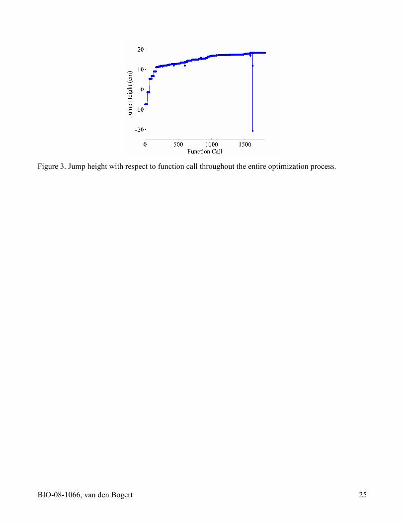
The optimization routine successfully achieved a center of mass jump height of 18.2 cm with

respect to a standing configuration (Figures 2 and 3). During the optimization, approximately 1800

movement simulations were performed, each requiring several thousand evaluations of the foot model.

A total of 51 optimization iterations were performed, with each iteration consisting of an initial model

evaluation followed by 32 forward simulations for gradient calculation, and a few more simulations to

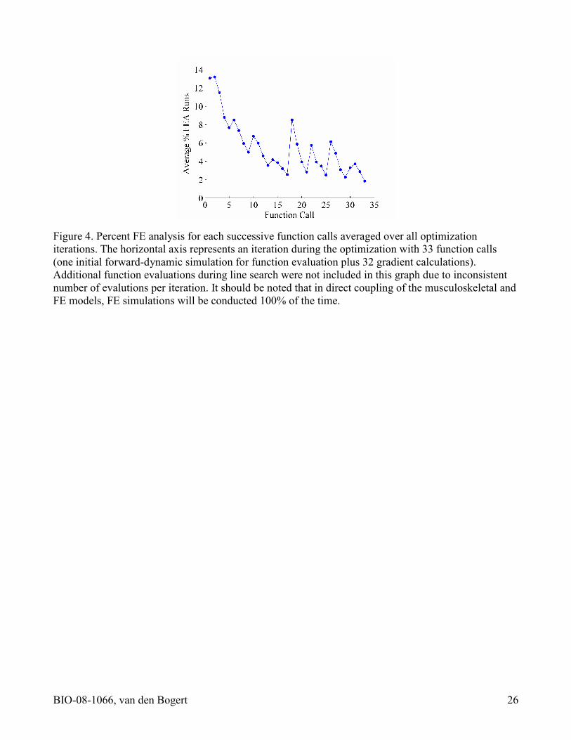
find the minimum for the iteration. Average percentage FEA runs were calculated over all 51 iterations

for initial function evaluation and calculation of individual components of the gradient (Figure 4). As

an iteration proceeded from function evaluation to gradient calculation, the number of FE simulations

decreased from 13% to 2% (Figure 4). This demonstrates that for the relatively small changes to the

control variables during the gradient calculations, the surrogate model was effective in learning a

specific area of the input space. Over the whole optimization, utilization of the surrogate model

resulted in an average reduction of 95% in the number of potential FE simulations, compared to direct

coupling between the FE model and musculoskeletal model (Figure 4). This reduction allowed the

movement prediction simulations to complete in approximately 4 weeks on a Linux based dual

processor Intel® Xeon 3.4 GHz machine with 6GB of memory.


The final database contained over 140,000 FE input/output sets. Each FE simulation required

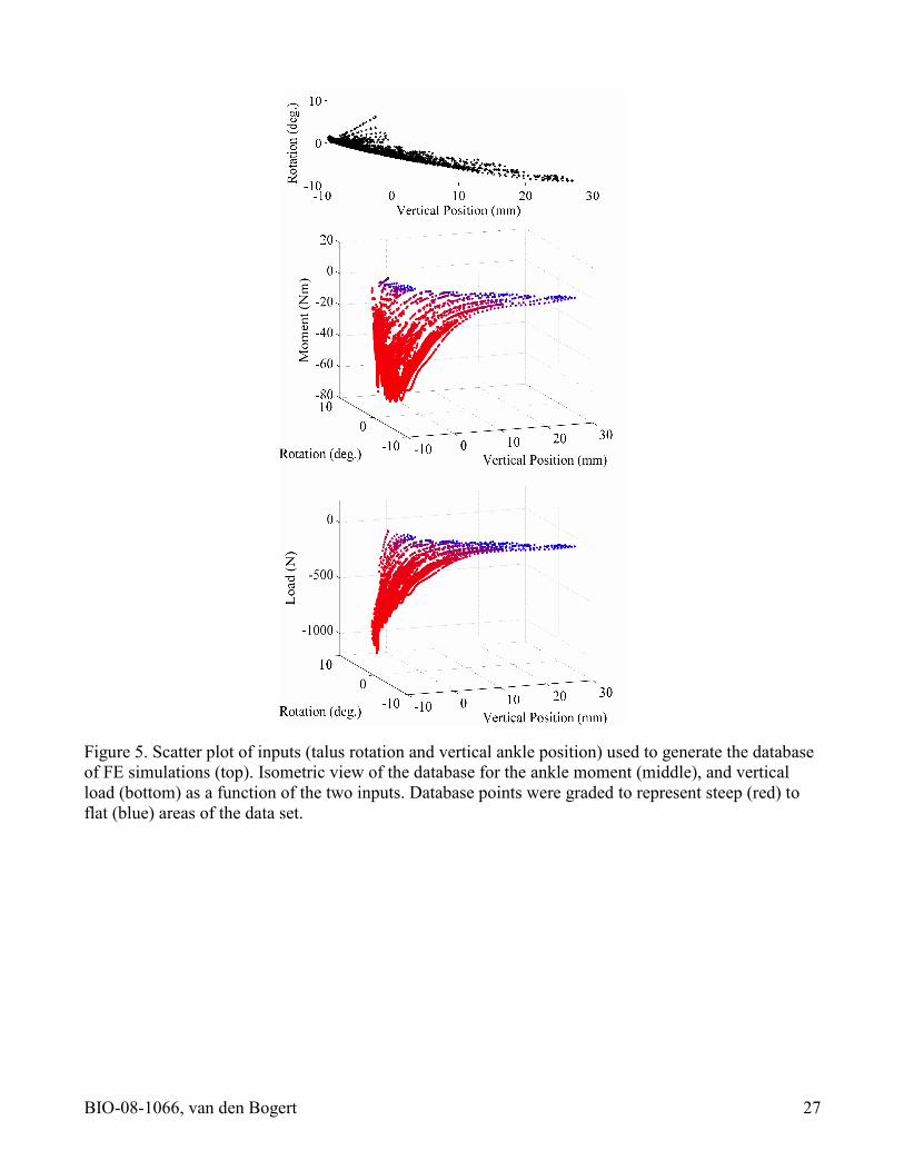
from 4 to 50 seconds to converge, depending on foot position and orientation. Color graded

input/output sets, based on a calculated slope using the 10 closest neighbors, highlighted the nonlinear

nature of the FE foot model (Figure 5). As this is a maximal effort simulation many data points were

required in high load, and thus very stiff, areas of the database. These points tended to be added in the

later stages of the movement optimization.

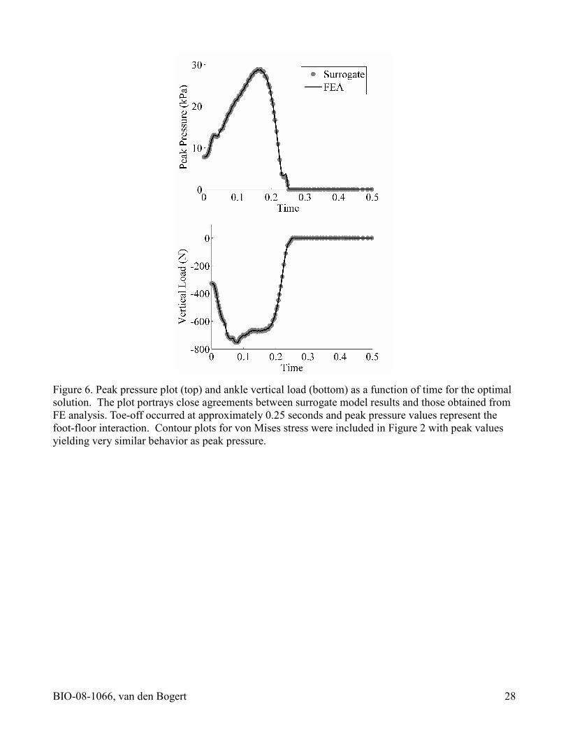
Accuracy of the surrogate model simulation was within 1 mm, obtained from the difference in

predicted jump height versus that obtained using FE simulations at every integration step. Optimal

neural excitation values were utilized during one forward simulation for the comparison. Surrogate

model predicted ankle reaction loads were acceptable when compared to the FE results throughout the

maximal height jumping simulation with RMS errors of 1.59 N for the vertical load and 0.244 Nm for

the plantar/dorsiflexion moment (Figure 6). Peak contact pressure and von Mises stresses were also

predicted throughout the jumping simulations and showed very good agreement between surrogate

model predicted values and FE results with RMS errors of 2 and 7 kPa (0.7% and 1.0% of maximum

value predicted during jumping), respectively.

Discussion

The presented modeling methodology successfully optimized jump height, using neural

excitation patterns as control variables, with a coupled musculoskeletal lower extremity model and FE

model of the foot. The FE model results were stored in a database, from which a surrogate model

attempted to predict subsequent FE results using local regression. When the estimated error of the

regression model was below the specified tolerance, the surrogate model output was used, otherwise a

new FE simulation was performed. As expected, this surrogate modeling scheme was able to gradually

eliminate the need for FE simulations, thus removing its computational cost that appears to be a

bottleneck in concurrent simulations of musculoskeletal movements and tissue deformations.


Furthermore, we have shown that the optimized jumping simulation using the surrogate foot model

sufficiently reproduced the same neuromuscular movement simulation directly coupled to the actual FE

model. Finally, we demonstrated that the surrogate modeling method provided good estimates of tissue

level variables, such as peak stress.

Maximal height jumping has been extensively studied in the literature and was also chosen for

this study because of its straightforward objective to be used as a test problem. Utilizing two-

dimensional models, Pandy et al. [27] achieved a jump height of 33 cm and van Soest et al. [28] a

height of 39.2 cm, with jump height defined by the vertical displacement of the center of mass relative

to the standing configuration. Comparing to the jump height of 18.2 cm in this study, the difference in

performance may be partly due to differences in muscle properties, including generally lower

maximum force producing capability for individual muscles of our study. Additional differences

include choice of control variables and the assumption of frictionless contact, which has been shown to

reduce predicted jump height [29]. Passive toe flexion also likely reduced the maximum achievable

jump height but we do not exclude the possibility that the gradient based SQP algorithm did not reach

to a global optimum. We should therefore consider this solution to be a local optimum and future work

will explore implementation using a global optimization routine. Nevertheless, this movement

optimization served as a good vehicle to demonstrate the feasibility of utilizing a multi-domain

simulation in a computationally intensive optimization of movement.

Further advances to the presented model will include incorporation of friction along with

validated 2D and 3D FE foot models. Interface loads and peak plantar pressures are influenced by

friction and the path taken to a given foot-ground orientation will affect the deformation of the plantar

tissue. Simulated jumping does not necessitate friction whereas other movement patterns such as gait

require the shear force supplied by the foot-ground interaction. When friction is included, path

dependent kinematic variable(s) will need to be incorporated into the estimation for accurate


approximations using a surrogate model. As one might expect, the dimension of the input space, and

the number of data points, will grow substantially as these features are included. The local regression

approach with adaptive sampling has the potential to avoid the "curse of dimensionality" by only

generating database points where needed. In practical applications, database management can be costly

and more sophisticated neighbor searching methods [30] will be useful as the complexity of the model

increases. Even in this study, with the final database size of over 140,000 points (Figure 5), database

management contributed significantly to the overall computational time.

Computational benefits of the surrogate model were assessed based on literature reported run

times and in-house simulations. Computation times for the optimization were not reported by Pandy et

al. [31] for two-dimensional jumping simulation. When the model was further developed in three

dimensions, the optimization routine for maximal jumping required between 1 and 2.5 months (for the

single processor machines) [32]. As more complex models and movement patterns are adopted the

computational expense further increases with one study citing 10,000 hours of computational time for a

gait cycle optimization [33]. Mclean et al. [24] reported 37 hours of computational time to simulate a

cutting maneuver and Neptune et al [34] required 660 hours to optimize a simulation of running. We

are aware that all these simulations considered different number of muscles, nodal parameters for

muscle excitations and were conducted using various computational platforms. Nevertheless, it is clear

that movement prediction takes considerable computational time even when one does not consider soft

tissue deformations through coupling. None of the studies cited above attempted concurrent

simulations. As stated earlier, the complete optimization routine for this study, even using a surrogate

model of foot deformations, required approximately 4 weeks of computational time (672 hours).

Computational expense for the forward simulations during the optimization routine varied dramatically,

from ~1 minute up to multiple hours, depending on the percentage of FE simulations and the database

size. It would not have been feasible to perform a movement optimization without the surrogate model.


One forward simulation using neural excitations from the optimized jump with direct FE analysis at

every integration point required 9.3 hours of computational time. If direct coupling had been

implemented for the movement prediction problem, FE analyses would be performed at every

integration point during the ~1800 function calls (each representing one forward simulation). The

associated expense for the complete optimization routine in this study would have required

approximately 698 days (16,752 hours) of computational time. Obviously, computational expense is a

central consideration when performing optimizations of movement patterns and becomes even more

important when soft-tissue deformation is included.

The performance of the locally weighted regression method will depend on algorithm

parameters, such as polynomial order, the number of neighbors considered, distance metric in input

space, and the tolerance value for adaptive sampling. For this study we selected a set of values that

provided reasonable local regression characteristics but an extensive parameter tuning is warranted to

decrease requested FE simulations without diminishing regression accuracy. Based on the errors found

in the surrogate model after completion of the movement optimization, we suspect that the cross

validation error estimates are overly pessimistic and that fewer FE simulations, possibly by relaxing the

tolerances, would have been sufficient to achieve good results. While the 0.244 Nm RMS error for the

ankle moment output metric appeared to be relatively high, peak errors occurred at the high load areas

of the database and still represented less than one percent of the applied moment. Sensitivity of the

jump height and accuracy of the surrogate model to changes in the interpolation parameters remain a

future direction of this work. Regardless, the linear approximation method proved to be accurate, and

through successive refinement in the database, it reduced the potential number of FE simulations

during an optimization iteration by 95% (Figure 4). As a result, the disproportionate computational cost

associated with the FE model was overcome, while the coupled behavior of the musculoskeletal and

tissue models was retained. Implementing a higher order regression technique could lessen the


computational FE burden, and thus the number of database points, but may require more time to

perform each regression.

Exploration of the ankle-foot complex has clinical applications in the prevention of diabetic

foot ulceration. With the coupled simulations, we will be able to explore the closed loop interactions

between sensory loss, neuromuscular control, and tissue stress and damage. The proposed

methodology, however, is not limited to this specific case. Any coupled, computationally expensive

modeling system could potentially benefit from a surrogate modeling approach. The complex behavior

of the knee would be a very good application where soft-tissue effects and joint level mechanics could

be predicted. Traditionally, computational models of the knee have required substantial resources and

boundary conditions that have not included musculoskeletal loading. Models of shoulder, hip and other

joints of interest could also be developed. Of particular clinical interest, the defined geometry and

material behavior of joint replacements would be well-suited to this method. Other applications in

biomechanics could include tissue-fluid interactions and coupling of cellular mechanics to tissue and

organ level models.

Direct coupling of finite element analysis to a single forward dynamics of a musculoskeletal

model has been shown to be possible [17]. However, predictive simulations that require multiple

solutions of the forward dynamics problem can only be possible with a cost-effective approach. To the

author’s knowledge, this is the first study to complete a predictive optimization of an active movement

with a coupled musculoskeletal and FE model of tissue level mechanics. A surrogate modeling

technique was developed to efficiently and adaptively predict the joint reaction loads and important

soft-tissue conditions of a corresponding FE model. Far less simplification of joint behavior versus

traditional musculoskeletal modeling is an important benefit of this method, and the ability to utilize

and predict tissue and joint mechanics adds clinical insight. This optimized muscle-loaded simulation

helps to further advance the state of musculoskeletal modeling and is an important step toward


development of musculoskeletal simulation strategies more aware of tissue deformations.

Acknowledgments

This study is supported by the National Institutes of Health grant 1 R01 EB006735-01. The authors

would like to thank Scott Sibole for developing the finite element model of the foot and Anna

Fernandez and Marko Ackermann for initial work on the jump optimizations.

References

[1] Huiskes, R. and Chao, E. Y. A survey of finite element analysis in orthopedic biomechanics: the

first decade. J. Biomech. 16(6):385-409, 1983.

[2] Gilbertson, L. G., Goel, V. K., Kong, W. Z. and Clausen, J. D. Finite element methods in spine

biomechanics research. Crit. Rev. Biomed. Eng. 23(5-6):411-473, 1995.

[3] Pandy, M. G. Computer modeling and simulation of human movement. Annu. Rev. Biomed. Eng.

3:245-73, 2001.

[4] Anderson, D. D., Goldsworthy, J. K., Li, W., Rudert, M. J., Tochigi, Y. and Brown, T. D. Physical

validation of a patient-specific contact finite element model of the ankle. J. Biomech. 40(8):1662-1669,

2007.

[5] Speirs, A. D., Heller, M. O., Duda, G. N. and Taylor, W. R. Physiologically based boundary

conditions in finite element modelling. J. Biomech. 40(10):2318-2323, 2007.

[6] Ellis, B. J., Debski, R. E., Moore, S. M., McMahon, P. J. and Weiss, J. A. Methodology and

sensitivity studies for finite element modeling of the inferior glenohumeral ligament complex. J.

Biomech. 40(3):603-612, 2007.

[7] Gardiner, J. C. and Weiss, J. A. Subject-specific finite element analysis of the human medial

collateral ligament during valgus knee loading. J. Orthop. Res. 21(6):1098-1106, 2003.

[8] Phatak, N. S., Sun, Q., Kim, S., Parker, D. L., Sanders, R. K., Veress, A. I., Ellis, B. J. and Weiss, J.

A. Noninvasive determination of ligament strain with deformable image registration. Ann. Biomed.

Eng. 35(7):1175-1187, 2007.

[9] Weiss, J. A., Gardiner, J. C., Ellis, B. J., Lujan, T. J., and Phatak, N. S. Three-dimensional finite

element modeling of ligaments: technical aspects. Med. Eng. Phys. 27:845-61, 2005.

[10] Yao, J., Salo, A. D., Lee, J. and Lerner, A. Sensitivity of tibio-menisco-femoral joint contact

behavior to variations in knee kinematics. J Biomech 41(2):390-398, 2008.

[11] Bourel, B., Combescure, A. and Valentin, L. D. Handling contact in multi-domain simulation of

automobile crashes. Finite. Elem. Anal. Des. 42(8):766-779, 2006.

[12] Gravouil, A. and Combescure, A. Multi-time-step and two-scale domain decomposition method

for non-linear structural dynamics. International Journal for Numerical Methods in Engineering

58(10):1545-1569, 2003.

[13] Kunzelman, K. S., Einstein, D. R. and Cochran, R. P. Fluid-structure interaction models of the

mitral valve: function in normal and pathological states. Philos. Trans. R. Soc. Lond. B. Biol. Sci.

362(1484):1393-1406, 2007.

[14] Nicosia, M. A., Cochran, R. P., Einstein, D. R., Rutland, C. J. and Kunzelman, K. S. A coupled

fluid-structure finite element model of the aortic valve and root. J. Heart Valve Dis. 12(6):781-789,

2003.

[15] Rassaian, M. and Lee, J. Generalized multi-domain method for fatigue analysis of interconnect

structures. Finite Elem. Anal. Des. 40(7):793-805, 2004.


[16] Besier, T. F., Gold, G. E., Beaupre, G. S., and Delp, S.L. A modeling framework to estimate

patellofemoral joint cartilage stress in vivo. Med Sci Sports Exerc. 37:1924-1930, 2005

[17] Koolstra, J. H. and van Eijden, T. M. G. J. Combined finite-element and rigid-body analysis of

human jaw joint dynamics. J. Biomech. 38(12):2431-2439, 2005.

[18] Bei, Y. and Fregly, B. J. Multibody dynamic simulation of knee contact mechanics. Med. Eng.

Phys. 26(9):777-789, 2004

[19] McLean, S.G., Huang, X., Su, A., and van den Bogert, A.J. Sagittal plane biomechanics cannot

injure the ACL during sidestep cutting. Clin. Biomech. 19(8):828-838, 2004.

[20] Lin, Y., Farr, J., Carter, K. and Fregly, B. J. Response surface optimization for joint contact model

evaluation. J. Appl. Biomech. 22(2):120-130, 2006.

[21] Atkeson, C. G., Moore, A. W. and Schaal, S. Locally weighted learning for control. Artif. Intell.

Rev. 11(1-5):75-113, 1997.

[22] Gerritsen, K. G., van den Bogert, A. J., Hulliger, M. and Zernicke, R. F. Intrinsic muscle properties

facilitate locomotor control - a computer simulation study. Motor Control 2(3):206-220, 1998.

[23] Hardin, E. C., Su, A. and van den Bogert, A. J. Foot and ankle forces during an automobile

collision: the influence of muscles. J. Biomech. 37(5):637-44, 2004.

[24] McLean, S. G., Su, A. and van den Bogert, A. J. 2003. Development and validation of a 3-D model

to predict knee joint loading during dynamic movement. J. Biomech. Eng. 125(6) 864-74.

[25] Erdemir A., Viveiros M. L., Ulbrecht J. S. and Cavanagh P. R. An inverse finite-element model of

heel-pad indentation. J. Biomech. 39(7):1279-86, 2006.

[26] Birattari, M., Bontempi, G. and Bersini, H. Lazy learning meets the recursive least squares

algorithm. Proceedings of the 1998 conference on Advances in neural information processing systems

II, MIT Press, Cambridge, MA, USA: 375-381, 1999.

[27] Pandy, M. G., Zajac, F. E., Sim, E. and Levine, W. S. An optimal control model for maximum-

height human jumping. J. Biomech. 23(12):1185-98, 1990.

[28] van Soest, A. J., Schwab, A. L., Bobbert M. F. and van Ingen Schenau G. J. The influence of the

biarticularity of the gastrocnemius muscle on vertical-jumping achievement. J. Biomech. 26:1-8, 1993.

[29] Bobbert, M. F., Houdijk, J. H. P., de Koning, J. J. and de Groot, G. From a one-legged vertical

jump to the speed-skating push-off: A stimulation study. J. Appl. Biomech. 18:28-45, 2002.

[30] Andoni, A. and Indyk, P. Near-optimal hashing algorithms for approximate nearest neighbor in

high dimensions. Commun. ACM. 51(1):117-122, 2008.

[31] Pandy, M. G. and Zajac, F. E. Optimal muscular coordination strategies for jumping. J. Biomech.

24(1):1-10, 1991.

[32] Anderson, F. C. and Pandy, M. G. A Dynamic optimization solution for vertical jumping in three

dimensions. Comput. Methods Biomech. Biomed. Engin. 2(3):201-231, 1999.

[33] Anderson, F. C. and Pandy, M. G. Dynamic optimization of human walking. J. Biomech. Eng.


123(5):381-90, 2001.

[34] Neptune, R. R., Wright, I. C. and Van Den Bogert, A. J. A method for numerical simulation of

single limb ground contact events: application to heel-toe running. Comput. Methods. Biomech.

Biomed. Engin. 3(4):321-334, 2000.


List of Figures

Figure 1. Coupled simulation of musculoskeletal movements and tissue deformations focusing on the

adaptive surrogate modeling approach. The components of q represent talus rotation and vertical

position and Q are the corresponding reactions. Note that when a finite element analysis is requested Q

is returned back to the musculoskeletal model for movement simulations and also to the surrogate

model with the corresponding q to expand the database. Data handling was performed in Matlab

(Mathworks, Inc., Natick, MA) where a script was developed to link the musculoskeletal model with

the FE through file input/output and with the surrogate model representation of the foot complex

directly.

Figure 2. Movement of the lower extremity during jumping obtained from the simulation with

maximum jump height prediction. Von Mises stress distributions within the FE model of the foot are

also illustrated for three time points during the simulation.

Figure 3. Jump height with respect to function call throughout the entire optimization process.

Figure 4. Percent FE analysis for each successive function calls averaged over all optimization

iterations. The horizontal axis represents an iteration during the optimization with 33 function calls

(one initial forward-dynamic simulation for function evaluation plus 32 gradient calculations).

Additional function evaluations during line search were not included in this graph due to inconsistent

number of evalutions per iteration. It should be noted that in direct coupling of the musculoskeletal and

FE models, FE simulations will be conducted 100% of the time.

Figure 5. Scatter plot of inputs (talus rotation and vertical ankle position) used to generate the database

of FE simulations (top). Isometric view of the database for the ankle moment (middle), and vertical

load (bottom) as a function of the two inputs. Database points were graded to represent steep (red) to

flat (blue) areas of the data set.

Figure 6. Peak pressure plot (top) and ankle vertical load (bottom) as a function of time for the optimal

solution. The plot portrays close agreements between surrogate model results and those obtained from

FE analysis. Toe-off occurred at approximately 0.25 seconds and peak pressure values represent the

foot-floor interaction. Contour plots for von Mises stress were included in Figure 2 with peak values

yielding very similar behavior as peak pressure.


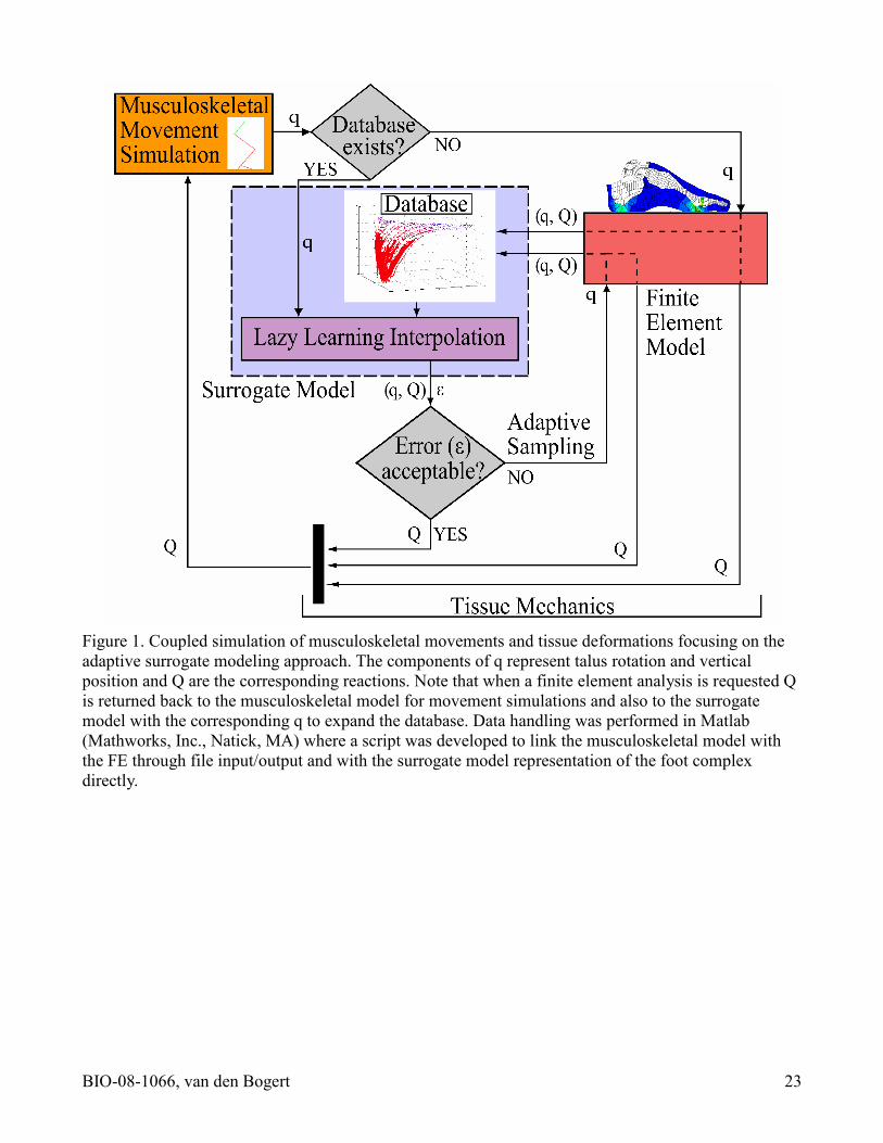
Figure 1. Coupled simulation of musculoskeletal movements and tissue deformations focusing on the

adaptive surrogate modeling approach. The components of q represent talus rotation and vertical

position and Q are the corresponding reactions. Note that when a finite element analysis is requested Q

is returned back to the musculoskeletal model for movement simulations and also to the surrogate

model with the corresponding q to expand the database. Data handling was performed in Matlab

(Mathworks, Inc., Natick, MA) where a script was developed to link the musculoskeletal model with

the FE through file input/output and with the surrogate model representation of the foot complex

directly.


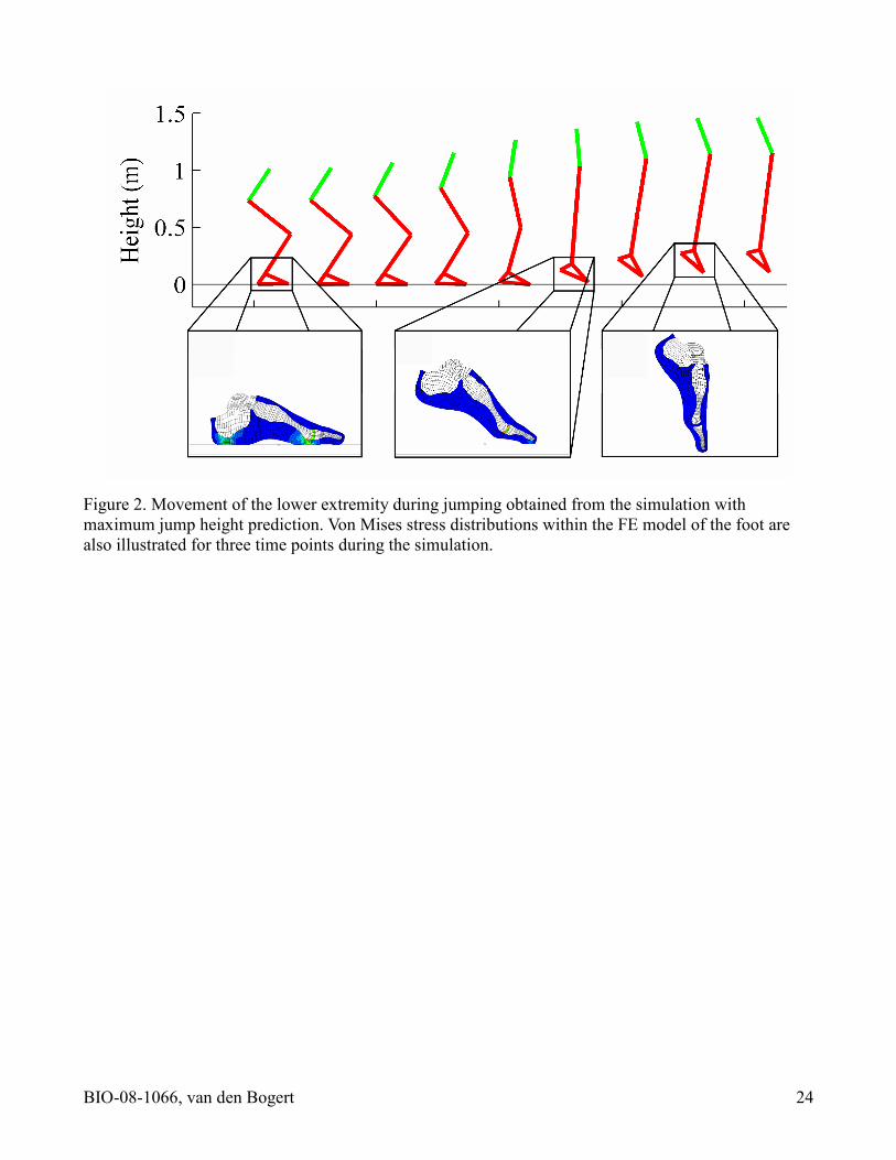
Figure 2. Movement of the lower extremity during jumping obtained from the simulation with

maximum jump height prediction. Von Mises stress distributions within the FE model of the foot are

also illustrated for three time points during the simulation.


Figure 3. Jump height with respect to function call throughout the entire optimization process.


Figure 4. Percent FE analysis for each successive function calls averaged over all optimization

iterations. The horizontal axis represents an iteration during the optimization with 33 function calls

(one initial forward-dynamic simulation for function evaluation plus 32 gradient calculations).

Additional function evaluations during line search were not included in this graph due to inconsistent

number of evalutions per iteration. It should be noted that in direct coupling of the musculoskeletal and

FE models, FE simulations will be conducted 100% of the time.


Figure 5. Scatter plot of inputs (talus rotation and vertical ankle position) used to generate the database

of FE simulations (top). Isometric view of the database for the ankle moment (middle), and vertical

load (bottom) as a function of the two inputs. Database points were graded to represent steep (red) to

flat (blue) areas of the data set.


Figure 6. Peak pressure plot (top) and ankle vertical load (bottom) as a function of time for the optimal

solution. The plot portrays close agreements between surrogate model results and those obtained from

FE analysis. Toe-off occurred at approximately 0.25 seconds and peak pressure values represent the

foot-floor interaction. Contour plots for von Mises stress were included in Figure 2 with peak values

yielding very similar behavior as peak pressure.

bio-08-1066, van den bogert 1 - simtk

Documents