Purdue UniversityPurdue e-PubsDepartment of Agricultural Economics FacultyPublications Department of Agricultural Economics

1-11-2013

Biofuels and Land Use Change: Applying RecentEvidence to Model EstimatesFarzad TaheripourDepartment of Agricultural Economics, Purdue University, tfarzad@purdue.edu

Wallace TynerDepartment of Agricultural Economics, Purdue University, wtyner@purdue.edu

Follow this and additional works at: https://docs.lib.purdue.edu/agedocs

This document has been made available through Purdue e-Pubs, a service of the Purdue University Libraries. Please contact epubs@purdue.edu foradditional information.

Taheripour, Farzad and Tyner, Wallace, "Biofuels and Land Use Change: Applying Recent Evidence to Model Estimates" (2013).Department of Agricultural Economics Faculty Publications. Paper 2.https://docs.lib.purdue.edu/agedocs/2

Appl. Sci. 2013, 3, 14-38; doi:10.3390/app3010014

applied sciences ISSN 2076-3417

www.mdpi.com/journal/applsci

Article

Biofuels and Land Use Change: Applying Recent Evidence to Model Estimates

Farzad Taheripour * and Wallace E. Tyner

Department of Agricultural Economics, Purdue University, 403 West State St. West Lafayette,

IN 47907-2056, USA; E-Mail: wtyner@purdue.edu

* Author to whom correspondence should be addressed; E-Mail: tfarzad@purdue.edu;

Tel.: +1-765-494-4612; Fax: +1-765-494-9176.

Received: 10 October 2012; in revised form: 4 December 2012 / Accepted: 6 January 2013 /

Published: 11 January 2013

Abstract: Biofuels impact on global land use has been a controversial yet important topic.

Up until recently, there has not been enough biofuels to have caused major land use

change, so the evidence from actual global land use data has been scant. However, in the

past decade, there have been 72 million hectares added to global crop cover. In this

research we take advantage of this new data to calibrate the Global Trade Analysis Project

(GTAP) model and parameters. We make two major changes. First, we calibrate the land

transformation parameters (called constant elasticity of transformation, CET) to global

regions so that the parameters better reflect the actual land cover change that has occurred.

Second, we alter the land cover nesting structure. In the old GTAP model, cropland,

pasture, and forest were all in the same nest suggesting, everything else being equal, that

pasture or forest convert to cropland with equal ease and cost. However, we now take

advantage of the fact that pasture converts to cropland at lower cost than forest. The paper

provides the theoretical and empirical justification for these two model improvements.

Then it re-evaluates the global land use impacts due to the USA ethanol program using the

improved model tuned with actual observations. Finally, it shows that compared to the old

model, the new model projects: (1) less expansion in global cropland due to ethanol

expansion; (2) lower U.S. share in global cropland expansion; (3) and lower forest share in

global cropland expansion.

OPEN ACCESS

Appl. Sci. 2013, 3 15

Keywords: general equilibrium; biofuels; land use changes; land transformation elasticity;

nesting structure

1. Introduction

Land use change induced by human activities is a major source of greenhouse gases (GHGs).

Houghton [1] estimated that about 1/3 of carbon emissions released to the atmosphere since 1850 has

resulted from land use change. Ramankutty and Foley [2] estimated that the average annual rate of

deforestation was about 4.25 MH during the time period of 1850–1990. The annual rate of

deforestation has increased to 8.3 MH in 1990s and then decreased to 5.2 MH during the past decade [3].

Expansion in cropland is the major source of land conversion and deforestation. Traditionally, the

expansion in cropland has occurred to satisfy the need for higher demands for food and fiber products.

During the past decades several countries around the world have launched biofuel programs to

produce renewable fuels from agricultural resources. Several papers have assessed the economic and

environmental impacts of these programs. The early papers published in this area suggested that the

USA corn ethanol program could cause major land use implications [4–6]. However, the more recent

studies find that the early estimates have overstated the land use implications of this program [7–13].

While research studies in this area have distinguished and examined the important factors which

determine the land use impacts of biofuels and their geographical distributions no attempt has been

made to validate the land use estimates due to biofuels in the face of actual observations [14]. The

reason is simple. Prior to the last couple of years, there was insufficient data on global land use change

during the biofuels boom era. However, now we have that data, and it can be used to better calibrate

prior estimates of land use change, which is the objective of this paper. The global biofuel programs,

particularly the USA and EU mandates, took off in the early 2000s. However, prior to the past

5–6 years the level of biofuel production was very low and there was no way to get any idea of land

use changes that might come about due to the much higher mandated levels of biofuels. In 2011, USA

corn ethanol production was over 14 billion gallons, near the Renewable Fuel Standard (RFS) level of

15 billion gallons stipulated for 2015. In this year Brazil also produced about 6 billion gallons of

sugarcane ethanol, and the EU members jointly produced more than 4 billion gallons of ethanol

equivalent of biofuels (including ethanol and biodiesel). Thus, with these large magnitudes of biofuel

production we should be able to see some impacts of land use change even if we still cannot isolate the

biofuels induced part of that change with precision.

The existing estimates for the indirect land use change (iLUC) emissions due to biofuels are usually

obtained from economic partial or general equilibrium models. To estimate iLUC emissions economic

models, one way or another, estimate induced land use changes due to biofuel production. A land

supply system which relates supply of different land types to their return or their land conversion costs

is a key and common component of economic models used in this area. The existing Computable

General Equilibrium (CGE) models usually use Constant Elasticity of Transformation (CET)

functional forms to define their land supply system. Land transformation elasticities are needed to

define a land supply system. These elasticities are difficult to directly estimate using econometric

Appl. Sci. 2013, 3 16

methods due to lack of sufficient quality data. In some circumstances the land transformation

elasticities can be retrieved from the exiting land supply elasticity estimates [15] or can be estimated

using simulated pseudo data [16]. A calibration or tuning practice is an alternative method which can

be applied to tune land transformation elasticities for large and global CGE models [13]. In this paper

we use observed information to tune the land transformation elasticities for the GTAP-BIO model.

This global CGE model, developed at the Center for Global Trade Analyses, has played a leading

role in estimating biofuel induced land use changes. Several studies have used this model to evaluate

iLUC emissions due to biofuels [7,10–12,17,18]. This model uses two different land transformation

elasticities to govern the supply of land in each region. The first transformation elasticity (named

ETL1) governs land allocation among managed forest, cropland, and pasture land. The second

transformation elasticity (named ETL2) distributes available croplands among alternative crops. In the

absence of regional empirical estimates for these elasticities, the model uses the same value for each of

these parameters for all regions presented in the model.

Using similar land transformation elasticities for all regions presented in the model cannot be

justified based on actual observations. As explained later on in this paper, historical observations

confirm that regional land use changes followed different patterns during the past two decades. For

example, historical data confirms the area of USA cropland remained constant during the past two

decades, but its distribution among crops has changed significantly during the same time period. This

indicates that no movement along land cover frontier has accrued in the USA during the past two

decades, but movement along the cropland frontier occurred frequently in this economy. On the other

hand, the area of cropland has expanded significantly in Sub Saharan Africa with relatively minor

changes in its distribution among crops over the past two decades. Clearly these two patterns are not

consistent with using the same land transformation elasticities for these two regions.

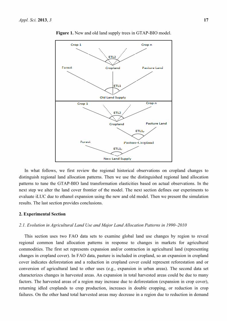
Furthermore, as shown in the top panel of Figure 1, the GTAP-BIO model puts three types of land

cover items (forest, pasture, and cropland) in one nest and implicitly assumes that the economic costs

of converting one hectare of forest to cropland is similar to the economic costs of converting one

hectare of pasture land to cropland and vice versa. This set up is another key deficiency of the

GTAP-BIO model. Including cropland, forest, and pasture land in the same nest could cause

systematic bias in land conversion processes among land cover types due to biofuel production. In

general this is not the case and often the opportunity costs of converting forest to cropland is higher

than the economic costs of converting pastureland to cropland.

In this paper we remove these two deficiencies. We tune the regional land transformation

elasticities based on actual historical observations on changes in land cover and distribution of

cropland among alternative crops during the past two decades. To accomplish this task we use

published data on cropland use around the world by the Food and Agricultural Organization (FAO) of

the United Nation over the period 1990–2010. We alters the land cover component of the land supply

tree, see the bottom panel of Figure 1, to have forest and pasture land in two different nests as

described later in this paper. Then we re-evaluate the global land use impacts due to the USA ethanol

program using the improved model tuned with actual observations. Finally, we show that compared to

the old model the new model projects: (1) less expansion in global cropland; (2) lower share for the

USA economy in global cropland expansion; (3) and lower forest share in global cropland expansion.

Appl. Sci. 2013, 3 17

Figure 1. New and old land supply trees in GTAP-BIO model.

In what follows, we first review the regional historical observations on cropland changes to

distinguish regional land allocation patterns. Then we use the distinguished regional land allocation

patterns to tune the GTAP-BIO land transformation elasticities based on actual observations. In the

next step we alter the land cover frontier of the model. The next section defines our experiments to

evaluate iLUC due to ethanol expansion using the new and old model. Then we present the simulation

results. The last section provides conclusions.

2. Experimental Section

2.1. Evolution in Agricultural Land Use and Major Land Allocation Patterns in 1990–2010

This section uses two FAO data sets to examine global land use changes by region to reveal

regional common land allocation patterns in response to changes in markets for agricultural

commodities. The first set represents expansion and/or contraction in agricultural land (representing

changes in cropland cover). In FAO data, pasture is included in cropland, so an expansion in cropland

cover indicates deforestation and a reduction in cropland cover could represent reforestation and or

conversion of agricultural land to other uses (e.g., expansion in urban areas). The second data set

characterizes changes in harvested areas. An expansion in total harvested areas could be due to many

factors. The harvested areas of a region may increase due to deforestation (expansion in crop cover),

returning idled croplands to crop production, increases in double cropping, or reduction in crop

failures. On the other hand total harvested areas may decrease in a region due to reduction in demand

Appl. Sci. 2013, 3 18

for crops, drought or other catastrophic events. In general, over a long time period total harvested area

and land cover move together. However in the short run they may diverge. In this section we also use

harvested areas to analyze changes in supply of land to alternative crops.

During the time period of 1990–2000 commodity markets were relatively stable, and in many

countries agricultural activities were under governmental support programs. The agricultural markets

experienced major changes in the next decade. Several countries (in particular, USA and EU members)

reduced or modified their agricultural support programs during this decade. Biofuel production began

to grow much faster around 2004 in many countries, especially USA, Brazil, and EU. Many counties,

especially China and India, observed significant food demand expansion due to rapid economic

growth. In addition, the crude oil price reached to its historical high with significant impacts on the

production costs of agricultural products. In response to these changes, crop prices went up

significantly and agricultural markets experienced major turbulences especially during the years

2008–2011. The higher commodity prices led to increases in cropland cover globally. The study of

regional land use changes during these time periods, in particular after 2004, is the key to tuning the

land transformation elasticities used in GTAP-BIO model.

The global area of agricultural land has increased by about 37.5 million hectares (MH) during the

past two decades. During this time period the area of global forest has decreased by about 135 MH.

These figures confirm land conversion along the land cover frontier at the global scale. On the other

hand, the global harvested area followed a relatively flat trend in the 1990s, and then it sharply

increased by about 71 MH during the next decades (from 1353 million hectares (MH) in 2000 to about

1424 MH in 2010 (Figure 2). This rapid growth in the global harvested area reflects major expansion

in the demand for agricultural products during the time period 2000–2010.

Figure 2. Global harvested area 1990–2010.

The allocation of cropland among alternative crops has changed significantly during the past two

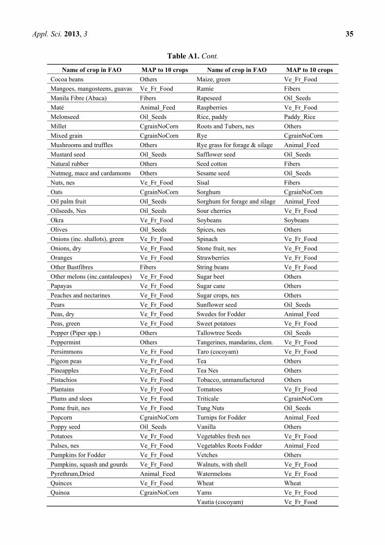
decades. Figure 3 summarizes changes in global harvested areas by crop for the past two decades (for

the list of crop categories and their member see Table A1 in Appendix A). This figure indicates

positive and large changes in the harvested areas of maize and oilseeds and negative and large changes

in the harvested areas of crop categories of wheat, other coarse grains, and animal feed. From these

observations we can conclude that global harvested area has increased significantly during 2000–2010.

However, the rate of land conversion from forest to agricultural land has decreased in this time period

compared to the time period of 1990–2000. Reduction in the area of global idled land, increase in

Appl. Sci. 2013, 3 19

double cropping, and reduction in crop failure could help explain the increase in harvested area while

forest cover has decreased less.

Figure 3. Changes in global harvested area by crops (figures are in million hectares).

Figure 4. Global harvested area by region trajectory.

Appl. Sci. 2013, 3 20

We now examine regional changes in agricultural land and harvested (the regional aggregation is

taken from GTAP-GIO model and is presented in Table B1 in Appendix B). Figure 4 represents

trajectories of harvested areas by region during the past two decades. In general, the 19 regions

presented in this figure can be divided into three groups in terms of land conversion among land cover

items and among alternative crops.

The first group includes regions or countries for which harvested areas have not changed

extensively during the past two decades. However, in these countries allocation of cropland among

alternative crops has typically changed over time. For example, during the past two decades the

harvested area of USA has remained relatively flat around 135 MH, with minor fluctuations. During

this time period (1990–2010) the agricultural land area of this county has decreased by about 5.5%, or

about 0.27% per year. Land conversion in this region has happened in favor of reforestation at a small

rate (about 0.4 MH per year) during the past two decades. Also, urbanization explains some of the loss

in agricultural land. On the other hand, in the USA allocation of cropland among the alternative crops

has significantly changed during the past two decades. During this time period the harvested areas of

soybeans and maize have increased sharply, while the harvested areas of animal feed crops and wheat

have decreased. This indicates that cropland has moved from one crop to another one easily in

response to the market forces in the US. Several other countries or regions including EU27, R_S_Asia,

and Oth_CES_CIS have followed this pattern.

This pattern of land use change can be interpreted as a negligible movement along the land cover

frontier and a major move along the cropland frontier as represented in the panel I of Figure 5. The left

side chart in this panel represents a typical land cover frontier with a small move from agriculture

towards forest (which represents the case of USA). This causes an insignificant inward shift in the

cropland cover on the right side chart in panel I. The right hand chart represents a major move along

the cropland frontier from crop type 1 to the crop type 2 as relative prices of the crops change,

represented by the two relative price lines.

The second group represents regions or countries for which harvested area has expanded

significantly during the past two decades. For example, the harvested area of Sub Saharan Africa has

increased at a rapid rate during the period of 1990–2010, from about 133 MH in 1990 to 165 MH in

2000 and 195 MH in 2010. Hence the harvested area of this region has increased by about 62 MH

(46%) during the past two decades. During this time period (1990–2010) the agricultural land area of

this region has increased by about 56 MH, and its forest area decreased by 75 MH.

In this region the harvested areas of crop categories of soybeans, animal feed, fiber, wheat, and

paddy rice remained constant at their small initial values. However, the harvested areas of crop

categories of other oilseeds, vegetable and fruits, other coarse grains (mainly sorghum), maize, and

other crops have followed upward trends in 1990s and 2000s. In particular, the harvested areas of

vegetable and fruits, other coarse grains, and other oilseeds have increased by 13, 10, and 6.6 MH in

1990s and by 10, 6.4, and 4.3 MH in 2000s.

The observed changes in the harvested area, expansions in agricultural land, and major

deforestation in Sub Saharan Africa confirms that in this region a major land conversion has happened

from forest to cropland, and the expanded croplands are used to expand production of certain crop

categories. This pattern of land use change can be interpreted as large movement along the land cover

frontier, for the case of this region in favor of cropland expansion. The expansion in cropland moves

Appl. Sci. 2013, 3 21

the cropland frontier to the right. The panel II of Figure 5 which represents a large movement along the

land cover frontier demonstrates the pattern of land use changes in this region. Several regions or

countries including S_o_America and Mala_Indo have followed this pattern.

Figure 5. Three patterns of land use changes.

Finally, consider the third group of countries or regions which fall somewhere in between these

polar cases. In this group some countries such as Canada, India, and C_C_Amer observed limited

changes in both land cover and cropland frontiers. On the other hand some countries in this group

observed land conversions along both frontiers. For example, the harvested area of Brazil has

Appl. Sci. 2013, 3 22

increased by about 14.1 MH during the past two decades. In this country the area of agricultural land

has increased by 23 MH and the forest area decreased by about 55 MH in the same time period. These

figures show that about 50% of deforestation in Brazil resulted in additions to the cropland area.

The harvested area of soybean has increased from 11.4 MH in 1990 to 13.6 MH in 2000 and

23.3 MH in 2010 in Brazil. The harvested area of maize has frequently fluctuated around 11 to 14 MH

during the past two decades. The harvested area of other crops (including sugarcane) followed an

upward trend during the past two decades and in particular in 2000s in this country. The harvested area

of sugarcane has increased from 4.3 MH in 1990 to 4.8 MH in 2000 and 9.1 MH in 2010. In general,

the harvested areas of paddy rice, wheat, fibers, and vegetable and fruits followed downward trends

during the time period of 1990 to 2010.

The observed changes in the harvested area and agricultural land in Brazil and changes in the

allocation of cropland among crops in this country demonstrate a mix of the first two extreme cases of

land use change. This pattern of land use change can be interpreted as a mix of changes along the land

cover and cropland frontiers. The panel III of Figure 5 which represents movements along the land

cover and cropland frontiers demonstrate the pattern of land use changes in this region. Several regions

or countries including Japan, E_Asia, and R_SE_Asia, followed this this pattern of land use changes.

The global harvested area has increased by about 30.6 MH since 2004, when biofuel began to

expand rapidly. Several countries such as S_S_Afr, CHIHKG, R_SE_Asia, and S_o_Amer made

major contributions to the expansion in global harvested area in this time period. On the other hand,

regions such as Russia, EU27, and MEAS_NAfr (Middle East and North Africa) lost a portion of their

harvested area since 2004. The reduction in the harvested area of Russia was about 18.1 MH in this

time period. A large portion of this reduction was due to crop failure in 2010.

The historical observations confirm that the expansion paths of maize and oilseeds have shifted up

in this time period in many regions. For example, the top panel of Figure 6 summarizes the increasing

expansion path of the share of maize in the USA harvested area during the past two decades and in

particular since 2004. This graph shows that share of maize in this region has jumped up significantly

during the biofuel era. As mentioned earlier, the expansion in maize and soybean harvested areas in the

USA caused reductions in harvested areas of other crops and did not lead to expanded cropland area. A

similar pattern can be observed in the EU region for the case of biodiesel. The bottom panel of Figure 6

shows that in this region the expansion in biodiesel production led to a jump in the share of harvested

areas of oilseeds, while total harvested area was fluctuating around 120 MH during the biofuel era.

In general since 2004 several countries such as S_S_Afr, CHIHKG, R_SE_Asia, and S_o_Amer

made major contributions to the expansion in global harvested area in this time period (Figure 7). On

the other hand, regions such as Russia, EU27, and MEAS_NAfr (Middle East and North Africa) lost a

portion of their harvested area since 2004 (Figure 7). The reduction in the harvested area of Russia was

about 18.1 MH in this time period. A large portion of this reduction was due to crop failure in 2010.

Appl. Sci. 2013, 3 23

Figure 6. USA and EU27 harvested areas and their oilseeds area share.

Figure 7. Change in harvested area by region, 2004–2010.

Appl. Sci. 2013, 3 24

2.2. Modifications in GTAP Land Transformation Elasticities

This section provides a framework to tune the GTAP land transformation elasticities with the

historical observed land used patterns. As mentioned in section 3 the regional observed trends in land

use patterns prior and after the boom in global biofuel industry are very similar, except that the area

shares of maize and oilseeds tends to be higher since 2004. For this reason we tune the GTAP land

transformation elasticities for the observed patterns during the time period of 2004–2010.

We begin the tuning process with the regional land cover elasticities. The historical changes in total

harvested area of a region is a good indication of changes in cropland cover over time, in particular

when they are in line with historical changes in forest area. The GTAP-BIO model assumes

ETL1 = −0.2 everywhere across the world. As noted in the supporting documents of Hertel et al. [7],

this relatively small value had been selected from the Ahmed et al. [15] calibration process. These

authors developed a calibration process to estimate aggregated cropland transformation elasticities as a

function of time based on Lubowski [19] who estimated land supply elasticities for the USA economy

using county level data observed in 1982, 1987, 1992, and 1997. Ahmed et al. [15] have shown that

the land cover transformation elasticity should be small for short to medium run time horizons. The

choice ETL = −0.2 is clearly made based on observations on the historical land use changes in USA

until 1997. While this figure fairly represents inflexibility in the USA land cover frontier, recent

observations confirm more inflexibility in USA land cover frontier at the aggregate level in recent

years. For example, recent evidence shows that cropland rent has increased faster than pasture rent in

recent years in USA, but the area of cropland remained relatively unchanged. The ratio of cropland

rent over pasture rent has increased gradually from about 8 in 2004 to 9.3 in 2010. This means that

land owners/farmers had the incentive to move their land from pasture to cropland. However, recent

observations indicate that the area of cropland has not increased in the USA in recent years. This

confirms a very small land transformation elasticity for the USA land cover frontier.

While data suggest very small land transformation elasticity for US, exiting evidence indicates

major movements in land cover in other regions. This means that a uniform and small value of land

transformation elasticity does not reflect actual regional observations. To tune this value to the

observed changes in land cover of each region, the 19 regions of GTAP-BIO model are ranked based

on their absolute value of annual average changes in harvested area since 2004. The results are

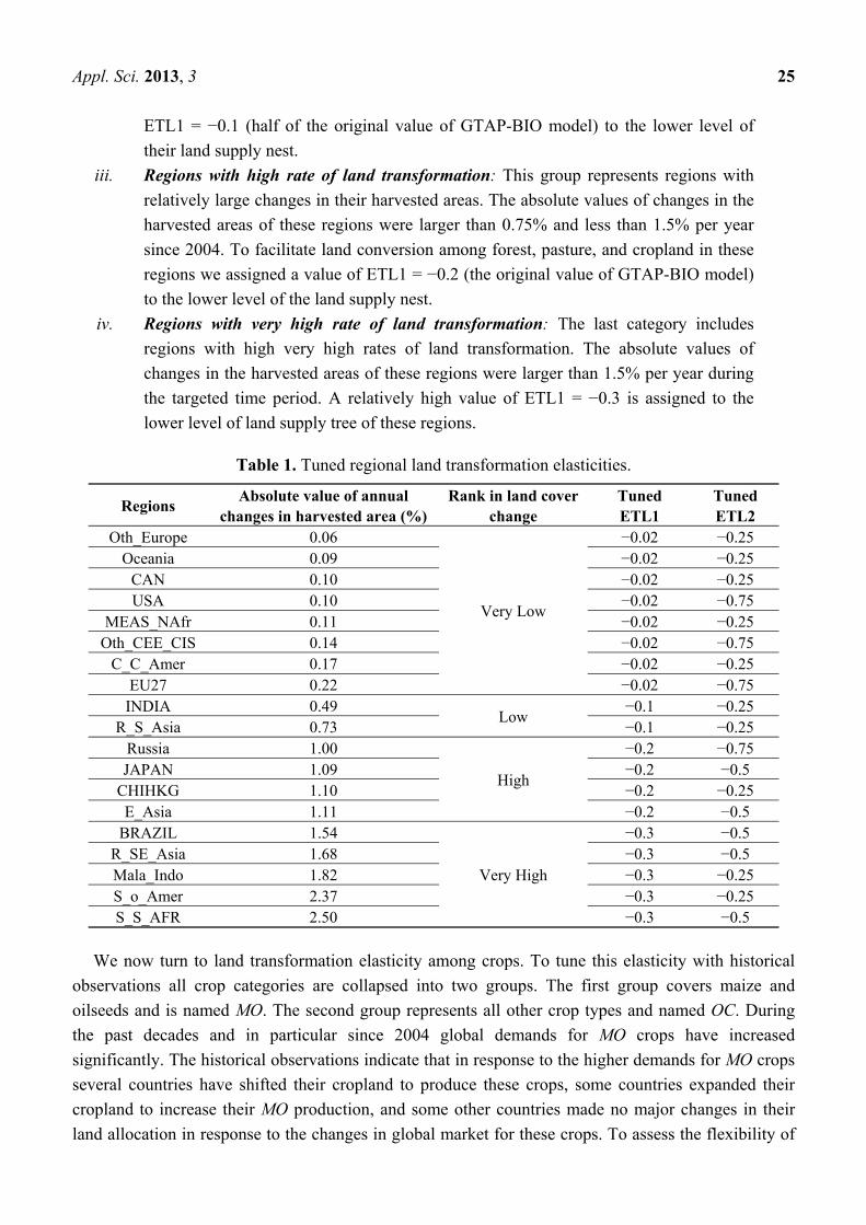
reported in Table 1. The 19 regions are divided into four categories based on the following schedule:

i. Regions with very low rate of land transformation: This category represents regions

with very limited changes in land cover during the time period of 2004–2010. The

absolute values of changes in the harvested areas of these regions were below 0.25%

per year after 2004. To limit land conversion among forest, pasture, and cropland in

these regions we assigned a value of ETL1 = −0.02 to the lower level of the land

supply nest.

ii. Regions with low rate of land transformation: This category represents regions with

relatively low annual rates of land transformation during the targeted time period. The

absolute value of changes in the harvested areas of these region where higher than

0.25% and lower than 0.75% since 2004. For these regions we assigned a value of

Appl. Sci. 2013, 3 25

ETL1 = −0.1 (half of the original value of GTAP-BIO model) to the lower level of

their land supply nest.

iii. Regions with high rate of land transformation: This group represents regions with

relatively large changes in their harvested areas. The absolute values of changes in the

harvested areas of these regions were larger than 0.75% and less than 1.5% per year

since 2004. To facilitate land conversion among forest, pasture, and cropland in these

regions we assigned a value of ETL1 = −0.2 (the original value of GTAP-BIO model)

to the lower level of the land supply nest.

iv. Regions with very high rate of land transformation: The last category includes

regions with high very high rates of land transformation. The absolute values of

changes in the harvested areas of these regions were larger than 1.5% per year during

the targeted time period. A relatively high value of ETL1 = −0.3 is assigned to the

lower level of land supply tree of these regions.

Table 1. Tuned regional land transformation elasticities.

Regions Absolute value of annual

changes in harvested area (%) Rank in land cover

change Tuned ETL1

Tuned ETL2

Oth_Europe 0.06

Very Low

−0.02 −0.25 Oceania 0.09 −0.02 −0.25

CAN 0.10 −0.02 −0.25 USA 0.10 −0.02 −0.75

MEAS_NAfr 0.11 −0.02 −0.25 Oth_CEE_CIS 0.14 −0.02 −0.75

C_C_Amer 0.17 −0.02 −0.25 EU27 0.22 −0.02 −0.75

INDIA 0.49 Low

−0.1 −0.25 R_S_Asia 0.73 −0.1 −0.25

Russia 1.00

High

−0.2 −0.75 JAPAN 1.09 −0.2 −0.5

CHIHKG 1.10 −0.2 −0.25 E_Asia 1.11 −0.2 −0.5

BRAZIL 1.54

Very High

−0.3 −0.5 R_SE_Asia 1.68 −0.3 −0.5 Mala_Indo 1.82 −0.3 −0.25 S_o_Amer 2.37 −0.3 −0.25 S_S_AFR 2.50 −0.3 −0.5

We now turn to land transformation elasticity among crops. To tune this elasticity with historical

observations all crop categories are collapsed into two groups. The first group covers maize and

oilseeds and is named MO. The second group represents all other crop types and named OC. During

the past decades and in particular since 2004 global demands for MO crops have increased

significantly. The historical observations indicate that in response to the higher demands for MO crops

several countries have shifted their cropland to produce these crops, some countries expanded their

cropland to increase their MO production, and some other countries made no major changes in their

land allocation in response to the changes in global market for these crops. To assess the flexibility of

Appl. Sci. 2013, 3 26

countries in their cropland frontier we rely on the regional changes in the harvested areas of MO and

OC crops.

To establish a benchmark consider the USA economy which shifted a big portion of its existing

cropland to produce more MO crops without expansion in its cropland area during the past two

decades and in particular since 2004. It is straight forward to evaluate the cropland transformation

elasticity for this economy using the concept of Arch Transformation Elasticity (ATE). To establish

the theoretical base consider Figure 8 which represents moving over the cropland frontier from point A

to point B to produce more MO crops. For this movement the size of ATE can be obtained from the

following relationship: · . For example, suppose point A represents the year 2003

(one year before biofuel boom) and point B represents 2010. Then ATE = −0.86 for the USA economy

between 2003 and 2010. If we change the base to 2002 then ATE = −0.76 and if we change the end

year to 2009 then ATE = −0.67. Note that in calculating these values we dropped the term from the

above formula because XB were equal YB in recent years. All of these numbers are indeed around

ETL2 = −0.75 used in the latest versions of GTAP-BIO developed by Taheripour et al. [17] and

Tyner et al. [18]. We considered this value of ETL2 as the highest rate of land transformation for the

cropland cover. The cropland transformation elasticities of other regions are tuned with respect to this

benchmark. To accomplish this task the same high value of −0.75 is assigned to the ETL2 for EU,

Russia, and Oth_CEE_CIS regions, which observed limited or no expansion in their cropland and

moved their existing cropland to MO crops since 2004. On the other hand, for those regions which

experienced no major expansion in their cropland area and had no significant changes in their land

allocation among crops, we assigned a low value of −0.25 to their ETL2 rate. Several regions

including Canada, C_C_Amer, Oth_Europe, MEAS_NAfr, and Oceania fall in this group.

Figure 8. Moving towards MO crop without cropland expansion.

Finally, a test is developed to decide about the size of ETL2 for other countries which experienced

expansion in their cropland and observed changes in their cropland allocation among the MO and OC

crops. The test which is explained in Appendix C determines the sources of changes in the area of MO

crops in each region over time. The area of MO crop in each region could change due to two sources. It

can change either due to expansion in cropland or a combination of expansion in cropland and

switching from production of OC to MO crops. In each region, if the expansion occurred only due to

cropland expansion, then a limited value of −0.25 is assigned to ETL2 of that region, otherwise a value

of −0.5 is used. A full set of new regional ETL2 is presented in Table 1.

Appl. Sci. 2013, 3 27

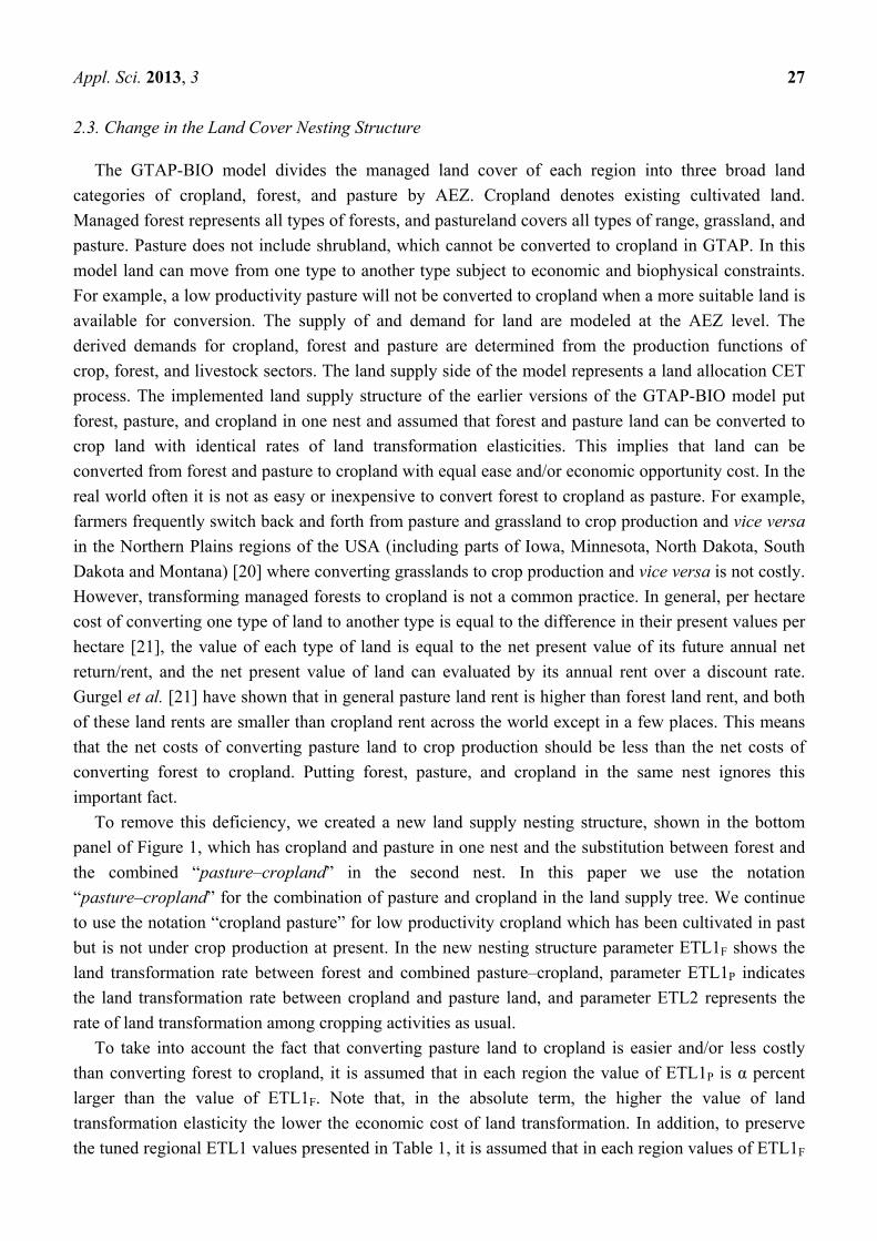
2.3. Change in the Land Cover Nesting Structure

The GTAP-BIO model divides the managed land cover of each region into three broad land

categories of cropland, forest, and pasture by AEZ. Cropland denotes existing cultivated land.

Managed forest represents all types of forests, and pastureland covers all types of range, grassland, and

pasture. Pasture does not include shrubland, which cannot be converted to cropland in GTAP. In this

model land can move from one type to another type subject to economic and biophysical constraints.

For example, a low productivity pasture will not be converted to cropland when a more suitable land is

available for conversion. The supply of and demand for land are modeled at the AEZ level. The

derived demands for cropland, forest and pasture are determined from the production functions of

crop, forest, and livestock sectors. The land supply side of the model represents a land allocation CET

process. The implemented land supply structure of the earlier versions of the GTAP-BIO model put

forest, pasture, and cropland in one nest and assumed that forest and pasture land can be converted to

crop land with identical rates of land transformation elasticities. This implies that land can be

converted from forest and pasture to cropland with equal ease and/or economic opportunity cost. In the

real world often it is not as easy or inexpensive to convert forest to cropland as pasture. For example,

farmers frequently switch back and forth from pasture and grassland to crop production and vice versa

in the Northern Plains regions of the USA (including parts of Iowa, Minnesota, North Dakota, South

Dakota and Montana) [20] where converting grasslands to crop production and vice versa is not costly.

However, transforming managed forests to cropland is not a common practice. In general, per hectare

cost of converting one type of land to another type is equal to the difference in their present values per

hectare [21], the value of each type of land is equal to the net present value of its future annual net

return/rent, and the net present value of land can evaluated by its annual rent over a discount rate.

Gurgel et al. [21] have shown that in general pasture land rent is higher than forest land rent, and both

of these land rents are smaller than cropland rent across the world except in a few places. This means

that the net costs of converting pasture land to crop production should be less than the net costs of

converting forest to cropland. Putting forest, pasture, and cropland in the same nest ignores this

important fact.

To remove this deficiency, we created a new land supply nesting structure, shown in the bottom

panel of Figure 1, which has cropland and pasture in one nest and the substitution between forest and

the combined “pasture–cropland” in the second nest. In this paper we use the notation

“pasture–cropland” for the combination of pasture and cropland in the land supply tree. We continue

to use the notation “cropland pasture” for low productivity cropland which has been cultivated in past

but is not under crop production at present. In the new nesting structure parameter ETL1F shows the

land transformation rate between forest and combined pasture–cropland, parameter ETL1P indicates

the land transformation rate between cropland and pasture land, and parameter ETL2 represents the

rate of land transformation among cropping activities as usual.

To take into account the fact that converting pasture land to cropland is easier and/or less costly

than converting forest to cropland, it is assumed that in each region the value of ETL1P is α percent

larger than the value of ETL1F. Note that, in the absolute term, the higher the value of land

transformation elasticity the lower the economic cost of land transformation. In addition, to preserve

the tuned regional ETL1 values presented in Table 1, it is assumed that in each region values of ETL1F

Appl. Sci. 2013, 3 28

and ETL1P deviate from the value of ETL1 of that region by plus and minus β, respectively. Under

these assumptions it is straight forward to show that: β= α/(200 + α). In this paper we assumed that

ETL1P is 20% larger than ETL1F to take into account the fact that converting forest to cropland is more

costly than converting pasture land to cropland. Given these assumptions the regional values for

ETL1F and ETL1P are obtained from the regional values of ETL1 presented in Table 1. The calculated

values for these land transformation values are presented in Table 2.

Table 2. Tuned regional land cover transformation elasticities.

Regions Rank in land cover change

Tuned ETL1 Tuned ETL1F Tuned ETL1P Tuned ETL2

Oth_Europe

Very Low

−0.02 −0.018 −0.0218 −0.25 Oceania −0.02 −0.018 −0.0218 −0.25 CAN −0.02 −0.018 −0.0218 −0.25 USA −0.02 −0.018 −0.0218 −0.75 MEAS_NAfr −0.02 −0.018 −0.0218 −0.25 Oth_CEE_CIS −0.02 −0.018 −0.0218 −0.75 C_C_Amer −0.02 −0.018 −0.0218 −0.25 EU27 −0.02 −0.018 −0.0218 −0.75 INDIA

Low −0.1 −0.0909 −0.1091 −0.25

R_S_Asia −0.1 −0.0909 −0.1091 −0.25 Russia

High

−0.2 −0.1818 −0.2182 −0.75 JAPAN −0.2 −0.1818 −0.2182 −0.5 CHIHKG −0.2 −0.1818 −0.2182 −0.25 E_Asia −0.2 −0.1818 −0.2182 −0.5 BRAZIL

Very High

−0.3 −0.2727 −0.3273 −0.5 R_SE_Asia −0.3 −0.2727 −0.3273 −0.5 Mala_Indo −0.3 −0.2727 −0.3273 −0.25 S_o_Amer −0.3 −0.2727 −0.3273 −0.25 S_S_AFR −0.3 −0.2727 −0.3273 −0.5

3. Results and Discussion

3.1. Land Use Impacts of USA Ethanol Mandate

Several studies have used the GTAP-BIO model which operates based on a land supply tree with a

one-nest land cover structure and implements uniform land transformation elasticity values of

ETL1 = −0.2 and ETL2 = −0.5 (or recently ETL2 = −0.75) to evaluate the land use impacts of the USA

ethanol mandate. The results from these studies indicate that around 50 percent of the expansion in

global cropland due to USA ethanol occurs in the USA and that much of that is forest. The following

experiments show that moving from this set up to a new GTAP-BIO model which operates based on a

land supply tree with a two-nest land cover structure and implements regional land transformation

elasticities obtained from regional-historical observations could entirely alter this picture To analyze

the impacts of this transition on estimates of induced land use changes due to USA ethanol production

the following four experiments are designed and simulated:

Appl. Sci. 2013, 3 29

Experiment A. An increase in corn ethanol production from its 2004 level (3.41 billion

gallons [BG]) to 15 BG, using a land supply tree including a one-nest land cover structure

with uniform land transformation rates of ETL1 = −0.2 and ETL2 = −0.75 across the world.

Experiment B. An increase in corn ethanol production from its 2004 level (3.41 billion

gallons [BG]) to 15 BG, using a land supply tree including a one-nest land cover structure

with regional land transformation rates presented in Table 1.

Experiment C. An increase in corn ethanol production from its 2004 level (3.41 billion

gallons [BG]) to 15 BG, using a land supply tree including a two-nest land cover structure

with uniform land transformation rates of ETL1 = −0.2 and ETL2 = −0.75 across the world

while we assume in each region ETL1P is 20% larger than ETL1F.

Experiment D. An increase in corn ethanol production from its 2004 level (3.41 billion

gallons [BG]) to 15 BG, using a land supply tree including a two-nest land cover structure

with regional land transformation rates presented in Table 2.

To implement these experiments the GTAP-BIO modeling framework used in Tyner et al. [18] is

modified to handle the new land supply nesting structure with regional land transformation elasticities.

The land use consequences of the first two experiments A and B are presented and compared in Table 3.

Table 3. Induced land use changes due to USA ethanol mandate with one-nest land cover:

Uniform versus regional land transformation rates (figures are in 1000 hectares).

Regions

Experiment A: Uniform land transformation

rates of ETL1 = −0.2 and ETL2 = −0.75

Experiment B: Regional land

transformation rates Presented in Table 1

Forest Cropland Pasture Forest Cropland Pasture

USA −357.4 1033.3 −675.8 −91.6 155.7 −64.1

EU27 −85.8 136.2 −50.4 −21.2 33.6 −12.5

BRAZIL −3.6 91.6 −88.0 21.7 152.1 −173.8

CAN −123.9 184.5 −60.6 −29.4 41.0 −11.7

JAPAN −3.0 3.5 −0.5 −5.3 5.3 0.0

CHIHKG 17.1 59.4 −76.4 −13.2 89.7 −76.5

INDIA −2.2 5.2 −3.0 −7.4 10.7 −3.3

C_C_Amer 34.8 22.3 −57.1 1.8 5.3 −7.0

S_o_Amer 85.8 67.1 −152.9 45.5 111.8 −157.3

E_Asia 4.3 0.8 −5.1 2.2 1.5 −3.7

Mala_Indo 8.2 −4.6 −3.6 1.4 1.6 −3.0

R_SE_Asia 2.5 2.8 −5.3 −12.3 14.4 −2.1

R_S_Asia −2.0 24.9 −23.0 −3.2 23.5 −20.3

Russia 194.3 9.5 −203.9 94.3 52.1 −146.4

Oth_CEE_CIS −22.6 110.3 −87.7 −8.8 27.5 −18.8

Oth_Europe −0.1 1.7 −1.6 −0.3 0.4 −0.1

MEAS_NAfr −0.1 89.6 −89.5 −0.1 21.1 −21.0

S_S_AFR −48.7 284.3 −235.7 −213.9 470.5 −256.6

Oceania −0.9 89.2 −88.3 −0.9 16.8 −15.9

Total −303.3 2211.7 −1908.4 −240.6 1234.6 −994.0

Cropland Pasture

USA −1218.6 −1793.7

Brazil −271.5 −221.2

Appl. Sci. 2013, 3 30

Table 3 indicates that experiment B with the new regional land transformation rates projects an

expansion in global cropland by about 1.2 MH, which is significantly smaller (by 44%) than the

corresponding figure obtained from experiment A with uniform land transformation values. The

geographical distribution of induced cropland expansion indicates the share of USA changes from 47%

to 13% when we use the regional parameters. We checked to see if there was a significant yield

increase due to intensification from the CET parameter change, and found that the changes were small

in all regions. The shares of EU27, Canada, also fall significantly. On the other hand the shares of

several other regions (in particular, S_S_AFR and S_o_Amer) go up.

Incorporation of the regional land transformation elasticities increases the share of forest in

expanded cropland from 13.7% to 19.5% at the global scale. On the other hand, in the USA, cropland

pasture conversion increases significantly, by more than 0.5 MH (or 47%).

Table 4. Induced land use changes due to USA ethanol mandate with two-nest land cover:

Uniform versus regional land transformation rates (figures are in 1000 hectares).

Regions

Experiment C: Uniform land transformation rates of

ETL1F = −0.1818, ETL1P = −0.2182, and ETL2 = −0.75

Experiment D: Regional land

transformation rates Presented in

Table 2

Forest Cropland Pasture Forest Cropland Pasture

USA −243.0 1055.9 −812.9 −64.8 157.4 −92.7

EU27 −73.3 137.2 −64.0 −14.7 33.6 −18.8

BRAZIL 45.2 101.0 −146.3 62.5 156.7 −219.2

CAN −110.4 176.1 −65.6 −25.4 40.1 −14.8

JAPAN −2.9 3.5 −0.6 −5.0 5.2 −0.1

CHIHKG 21.9 60.2 −82.2 −1.7 88.6 −86.8

INDIA −2.5 5.7 −3.2 −7.0 10.5 −3.5

C_C_Amer 38.1 22.4 −60.5 4.5 5.4 −9.9

S_o_Amer 100.2 72.1 −172.3 68.9 114.4 −183.3

E_Asia 4.0 0.9 −5.0 2.2 1.5 −3.8

Mala_Indo 7.2 −3.9 −3.3 0.9 2.1 −3.0

R_SE_Asia 2.0 3.1 −5.2 −11.8 14.4 −2.5

R_S_Asia −1.9 26.2 −24.2 −3.1 24.7 −21.6

Russia 176.1 18.5 −194.7 87.3 58.0 −145.3

Oth_CEE_CIS −21.3 114.8 −93.5 −7.4 28.8 −21.4

Oth_Europe −0.3 1.9 −1.7 −0.2 0.4 −0.2

MEAS_NAfr 0.5 92.8 −93.3 0.2 21.8 −21.9

S_S_AFR −14.8 273.0 −258.2 −167.1 461.8 −294.7

Oceania −0.1 93.6 −93.5 −0.5 17.9 −17.3

Total −74.9 2255.1 −2180.2 −82.4 1243.2 −1160.8

Cropland Pasture

USA −1195.4 −1788.5

Brazil 213.4 −213.9

Consider now the difference between the results obtained from experiments A (in Table 3) and C

(in Table 4). Both experiments are built based on uniform land transformation elasticities, but the

former uses a one-nest land cover and the latter uses a two-nest land cover with different values for

Appl. Sci. 2013, 3 31

pasture–cropland and the combination of pasture–cropland and forest. These two experiments project

very similar patterns for cropland expansion; however the two-nest model estimates a significantly

smaller share for forest in expanded cropland. The share of forest in global expanded cropland

decreases from 14% to 3%. This indicates that using a two-nest land cover only affects the share of

forest in expanded cropland due to ethanol production.

We now move to experiment D (Table 4) which includes both regional land transformation

elasticities and a two-nest land cover structure. Compared to experiment C, this experiment projects a

significantly smaller cropland expansion, by about 45%. And compared to experiment B, it projects a

major drop in the share of forest in cropland expansion, 20% in experiment B versus 7% in experiment

D. Finally, in comparing experiments A and D one can see that using a two-nest structure with regional

land transformation elasticities reduces the magnitude of cropland expansion by about 45%, and

decreases the share of forest in cropland expansion to 7%.

In conclusion, these analyses show that moving towards regional land transformation elasticities

reduces the magnitude of land conversion and using the two-nest land cover nesting structure

decreases the share of forest in land conversion. The combination of these two changes will contribute

to lower estimations for induced land use emissions due to ethanol production.

Consider now Figure 9 which compares the regional expansions in cropland areas obtained from

experiments A and D. This figure shows that the geographical distribution of cropland expansion

obtained from these two experiments are very different. Comparing Figures 7 and 9, it is clear that

experiment D does a much better job of representing the actual land use changes seen over the past six

years. There are still differences, but the new model which uses a two-nest land cover and implements

regional land transformation elasticities represents a significant improvement. And while the ethanol

shock is just one of many actual shocks, the land use changes likely play out in a similar way to the

idealized case with all shocks present.

Figure 9. Cropland expansion due to USA ethanol mandate based on experiments A and D.

Finally, compare Figures 10 and 11 which compare induced land use changes by land types for

experiments A and D. Figure 10 shows that in experiment A the ethanol expansion causes

Appl. Sci. 2013, 3 32

deforestation (by 0.36 MH) and conversion of pasture land (by 0.68 MH) in the US. But Figure 11,

which represents the results of experiment D, results in much lower USA land cover change due to

ethanol production (about 0.09 MH deforestations, 0.06 MH pasture conversions, and 0.15 MH

expansions in cropland). In addition, these figures show that the model with the new modifications

projects larger land conversions in Central and South America and Sub Saharan Africa.

Figure 10. Changes in global land cover in experiment A with original uniform land

transformation elasticities.

Figure 11. Changes in global land cover in experiment D with regional tuned land

transformation elasticities.

3.2. Land Use Emissions Due to Land Use Impacts of USA Ethanol Mandate

To measure land use emissions for the cases developed in this paper we rely on the land use

emissions factors reported for a 30-year time horizon by Plevin et al. [22]. These authors provided a

model which measures carbon fluxes due to land use changes induced by biofuel production at the

Appl. Sci. 2013, 3 33

AEZ level at a global scale. The estimated land emissions for the experiments A and D are about

20.3 g CO2eMJ−1 and 13.3 g CO2eMJ−1. With these figures we can conclude that using a two-nest land

cover structure and applying regional land transformation rates jointly reduce the calculated land use

emissions by about 18%, which is significantly smaller than the reduction in the estimated harvested

area. Part of the reason for this difference is the fact that these emission factors include cropland

pasture, and there is more cropland pasture conversion in experiment D than experiment A.

4. Conclusions

Previous versions of the GTAP-BIO model assume uniform values for the land transformation

elasticities for all regions worldwide. They also put forest, pasture and cropland in one nest and

assume forest and pasture land can be converted to cropland with identical land transformation

elasticities. In prior work there was not much land use change globally that could be used to calibrate

GTAP parameters, but in the past decade there has been substantial land cover change corresponding

to the period of the biofuels boom. The actual land use changes have varied significantly from one

region to another during the past two decades across the world. In addition, in real world converting

forest to cropland is more costly than converting pasture to cropland.

While we recognize that the CET parameter is not the only factor driving the extent and location of

land use change, it is one of the important parameters and one that can easily be varied by region. This

paper reviews changes in global cropland and indicates that during the past two decades countries

around the world have followed different land allocation patterns in the face of changes in markets for

crop products. While some regions have expanded their cropland significantly, other regions mainly

reallocated their existing cropland among alternative crops. This suggests that the land transformation

rates vary across the world. Based on these observations, uniform land transformation elasticities are

modified. In addition, the land cover nesting structure of the land supply tree is modified. In the new

land supply tree cropland and pasture are in one nest, and the combination of these two types of land

cover with forest are in another nest. Then the land use consequences of the USA ethanol mandate are

evaluated with these model and parameter changes.

The implemented experiments show that moving towards regional land transformation elasticities

reduces the magnitude of land conversion, and using the two-nest land cover nesting structure

decreases the share of forest in land conversion. The combination of these two changes reduces the

magnitude of cropland expansion by 45%, and decreases the share of forest in cropland expansion to

7%. The estimated land use emissions due to ethanol production falls by 18%. In addition, about

0.5 MH more cropland pasture will be converted to cropland due to these two modifications.

Acknowledgments

Partial funding for this research was provided by Office of Energy Products and New Uses,

U.S. Department of Agriculture, by the National Institute of Food And Agriculture, U.S. Department

of Agriculture, and also by the National Biodiesel Board.

Appl. Sci. 2013, 3 34

Appendix A

Table A1. List of crop categories and their members.

Name of crop in FAO MAP to 10 crops Name of crop in FAO MAP to 10 crops

Agave Fibres Nes Fibers Coconuts Oil_Seeds

Alfalfa for forage and silage Animal_Feed Coffee, green Others

Almonds, with shell Ve_Fr_Food Cow peas, dry Ve_Fr_Food

Anise, badian, fennel, corian. Animal_Feed Cranberries Ve_Fr_Food

Apples Ve_Fr_Food Cucumbers and gherkins Ve_Fr_Food

Apricots Ve_Fr_Food Currants Ve_Fr_Food

Arecanuts Ve_Fr_Food Dates Ve_Fr_Food

Artichokes Ve_Fr_Food Eggplants (aubergines) Ve_Fr_Food

Asparagus Ve_Fr_Food Fibre Crops Nes Fibers

Avocados Ve_Fr_Food Figs Ve_Fr_Food

Bambara beans Ve_Fr_Food Flax fibre and tow Fibers

Bananas Ve_Fr_Food Fonio CgrainNoCorn

Barley CgrainNoCorn forage Products Animal_Feed

Beans, dry Ve_Fr_Food Fruit Fresh Nes Ve_Fr_Food

Beans, green Ve_Fr_Food Fruit, tropical fresh nes Ve_Fr_Food

Beets for Fodder Animal_Feed Garlic Ve_Fr_Food

Berries Nes Ve_Fr_Food Ginger Others

Blueberries Ve_Fr_Food Gooseberries Ve_Fr_Food

Brazil nuts, with shell Ve_Fr_Food Grapefruit (inc. pomelos) Ve_Fr_Food

Broad beans, horse beans, dry Ve_Fr_Food Grapes Ve_Fr_Food

Buckwheat CgrainNoCorn Grasses Nes for forage;Sil Animal_Feed

Cabbage for Fodder Animal_Feed Green Oilseeds for Silage Animal_Feed

Cabbages and other brassicas Ve_Fr_Food Groundnuts, with shell Oil_Seeds

Canary seed CgrainNoCorn Hazelnuts, with shell Ve_Fr_Food

Carobs Ve_Fr_Food Hemp Tow Waste Fibers

Carrots and turnips Ve_Fr_Food Hempseed Oil_Seeds

Carrots for Fodder Animal_Feed Hops Others

Cashew nuts, with shell Ve_Fr_Food Jojoba Seeds Oil_Seeds

Cashewapple Ve_Fr_Food Jute Fibers

Cassava Ve_Fr_Food Kapok Fruit Fibers

Castor oil seed Oil_Seeds Karite Nuts (Sheanuts) Oil_Seeds

Cauliflowers and broccoli Ve_Fr_Food Kiwi fruit Ve_Fr_Food

Cereals, nes CgrainNoCorn Kolanuts Ve_Fr_Food

Cherries Ve_Fr_Food Leeks, other alliaceous veg Ve_Fr_Food

Chestnuts Ve_Fr_Food Leguminous for Silage Animal_Feed

Chick peas Ve_Fr_Food Leguminous vegetables, nes Animal_Feed

Chicory roots Ve_Fr_Food Lemons and limes Ve_Fr_Food

Chillies and peppers, dry Ve_Fr_Food Lentils Ve_Fr_Food

Chillies and peppers, green Ve_Fr_Food Lettuce and chicory Ve_Fr_Food

Cinnamon (canella) Others Linseed Oil_Seeds

Citrus fruit, nes Ve_Fr_Food Lupins Animal_Feed

Clover for forage and silage Animal_Feed Maize Grain_Maize

Cloves Animal_Feed Maize for forage and silage Animal_Feed

Appl. Sci. 2013, 3 35

Table A1. Cont.

Name of crop in FAO MAP to 10 crops Name of crop in FAO MAP to 10 crops

Cocoa beans Others Maize, green Ve_Fr_Food

Mangoes, mangosteens, guavas Ve_Fr_Food Ramie Fibers

Manila Fibre (Abaca) Fibers Rapeseed Oil_Seeds

Maté Animal_Feed Raspberries Ve_Fr_Food

Melonseed Oil_Seeds Rice, paddy Paddy_Rice

Millet CgrainNoCorn Roots and Tubers, nes Others

Mixed grain CgrainNoCorn Rye CgrainNoCorn

Mushrooms and truffles Others Rye grass for forage & silage Animal_Feed

Mustard seed Oil_Seeds Safflower seed Oil_Seeds

Natural rubber Others Seed cotton Fibers

Nutmeg, mace and cardamoms Others Sesame seed Oil_Seeds

Nuts, nes Ve_Fr_Food Sisal Fibers

Oats CgrainNoCorn Sorghum CgrainNoCorn

Oil palm fruit Oil_Seeds Sorghum for forage and silage Animal_Feed

Oilseeds, Nes Oil_Seeds Sour cherries Ve_Fr_Food

Okra Ve_Fr_Food Soybeans Soybeans

Olives Oil_Seeds Spices, nes Others

Onions (inc. shallots), green Ve_Fr_Food Spinach Ve_Fr_Food

Onions, dry Ve_Fr_Food Stone fruit, nes Ve_Fr_Food

Oranges Ve_Fr_Food Strawberries Ve_Fr_Food

Other Bastfibres Fibers String beans Ve_Fr_Food

Other melons (inc.cantaloupes) Ve_Fr_Food Sugar beet Others

Papayas Ve_Fr_Food Sugar cane Others

Peaches and nectarines Ve_Fr_Food Sugar crops, nes Others

Pears Ve_Fr_Food Sunflower seed Oil_Seeds

Peas, dry Ve_Fr_Food Swedes for Fodder Animal_Feed

Peas, green Ve_Fr_Food Sweet potatoes Ve_Fr_Food

Pepper (Piper spp.) Others Tallowtree Seeds Oil_Seeds

Peppermint Others Tangerines, mandarins, clem. Ve_Fr_Food

Persimmons Ve_Fr_Food Taro (cocoyam) Ve_Fr_Food

Pigeon peas Ve_Fr_Food Tea Others

Pineapples Ve_Fr_Food Tea Nes Others

Pistachios Ve_Fr_Food Tobacco, unmanufactured Others

Plantains Ve_Fr_Food Tomatoes Ve_Fr_Food

Plums and sloes Ve_Fr_Food Triticale CgrainNoCorn

Pome fruit, nes Ve_Fr_Food Tung Nuts Oil_Seeds

Popcorn CgrainNoCorn Turnips for Fodder Animal_Feed

Poppy seed Oil_Seeds Vanilla Others

Potatoes Ve_Fr_Food Vegetables fresh nes Ve_Fr_Food

Pulses, nes Ve_Fr_Food Vegetables Roots Fodder Animal_Feed

Pumpkins for Fodder Ve_Fr_Food Vetches Others

Pumpkins, squash and gourds Ve_Fr_Food Walnuts, with shell Ve_Fr_Food

Pyrethrum,Dried Animal_Feed Watermelons Ve_Fr_Food

Quinces Ve_Fr_Food Wheat Wheat

Quinoa CgrainNoCorn Yams Ve_Fr_Food

Yautia (cocoyam) Ve_Fr_Food

Appl. Sci. 2013, 3 36

Appendix B

Table B1. List of regions and their members.

Region Description Corresponding Countries in GTAP

USA United States Usa

EU27 European Union 27

aut, bel, bgr, cyp, cze, deu, dnk, esp, est, fin, fra,

gbr, grc, hun, irl, ita, ltu, lux, lva, mlt, nld, pol, prt,

rom, svk, svn, swe

BRAZIL Brazil Bra

CAN Canada Can

JAPAN Japan Jpn

CHIHKG China and Hong Kong chn, hkg

INDIA India Ind

C_C_Amer Central and Caribbean Americas mex, xna, xca, xfa, xcb

S_o_Amer South and Other Americas col, per, ven, xap, arg, chl, ury, xsm

E_Asia East Asia kor, twn, xea

Mala_Indo Malaysia and Indonesia ind, mys

R_SE_Asia Rest of South East Asia phl, sgp, tha, vnm, xse

R_S_Asia Rest of South Asia bgd, lka, xsa

Russia Russia Rus

Oth_CEE_CIS Other East Europe and Rest of Former

Soviet Union xer, alb, hrv, xsu, tur

R_Europe Rest of European Countries che, xef

MEAS_NAfr Middle Eastern and North Africa xme,mar, tun, xnf

S_S_AFR Sub Saharan Africa bwa, zaf, xsc, mwi, moz, tza, zmb, zwe, xsd, mdg,

uga, xss

Oceania Oceania countries aus, nzl, xoc

Appendix C

A Test to Determine Sources of Expansion in Harvested Area of Maize and Oilseeds (MO)

This appendix provides a simple test to determine the sources of expansion in the harvested areas of

MO crops when the harvested area of a region is expanded over time. In such a case the area of MO

crops can be expanded either through the expansion in total harvested area or shifting land from OC to

MO crop and vice versa. Consider Figure A1 which represents an expansion in a cropland frontier with

an upward shift from the initial position of F0 to the new position of F1. Suppose the initial allocation

of cropland among OC and MO crops is at point A on the F0 frontier. The allocation of cropland

among these two crop categories can be located on any point on the F1 frontier. Consider two possible

allocations of B and C. If the economy moves to point B then the line EB represents the expansion path

of harvested area in this case. If the economy moves to point C then the line EC represents the

expansion path. The line EB shows a monotonic expansion path. In this case the harvested areas of both

crops will increase proportionally due to the expansion in total harvested area. This line goes through

the origin and has no intercept. In this case no substitution among harvested areas will happen over

time. If the economy moves to point C, then the line EC represents a non-monotonic expansion path. In

Appl. Sci. 2013, 3 37

this case the harvested area of MO expands due to both expansion in total harvested area and moving

cropland from OC to MO.

Hence, if the expansion path of harvested area in a region represents a monotonic pattern, then one

can conclude no substitution among crops occurs. And if the expansion path of harvested area in a

region represents a non-monotonic pattern, then substitution among crops over time does happen.

Following this conclusion an expansion path is estimated for each of the regions which experienced

expansion in harvested area since 2004. Then for each region, if its expansion path was representing a

monotonic pattern a value of −0.25 is assigned to its cropland transformation rate, otherwise a value of

−0.5 is used.

Figure C1. Changes in global land over in experiment D.

References

1. Houghton, R.A. Revised estimates of the annual net flux of carbon to the atmosphere from

changes in land use and land management: 1850–2000. Tellus B 2003, 55, 378–390.

2. Ramankutty, N.; Foley, J.A. Estimating historical changes in global land cover: Croplands from

1700 to 1992. Global Biogeochem. Cycles 1999, 13, 997–1027.

3. Global Forest Resource Assessment 2010; Food and Agricultural Organization of the United

Nation: Rome, Italy, 2010.

4. Tokgoz, S.; Elobeid, A.; Fabiosa, J.F.; Hayes, D.J.; Babcock, B.A.; Yu, T.; Dong, F.; Hart, C.E.;

Beghin, J.C. Emerging Biofuels: Outlook of Effects on U.S. Grain, Oilseed, and Livestock

Markets; Staff Report 07-SR 101; Center for Agricultural and Rural Development: Ames, IA,

USA, 2007.

5. Kammen, D.M.; Farrell, A.E.; Plevin, R.J.; Jones, A.D.; Delucchi, M.A.; Nemet, G.F. Energy and

Greenhouse Impacts of Biofuels: A Framework for Analysis; Discussion paper 2007–2; Joint

Transport Research Centre: Berkeley, CA, USA, 2007.

6. Searchinger, T.; Heimlich, R.; Houghton, R.; Dong, F.; Elobeid, A.; Fabiosa, J.; Tokgoz, S.;

Hayes, D.; Yu, T. Use of U.S. Croplands for Biofuels Increases Greenhouse Gases Through

Emissions from Land-Use Change. Science 2008, 319, 1238–1240.

7. Hertel, T.; Golub, A.; Jones, J.; O’Hare, M.; Pelvin, R.; Kammen, D. Effects of USA Maize

Ethanol on Global Land Use and Greenhouse Gas Emissions: Estimating Market-Mediated

Responses. BioScience 2010, 60, 223–231.

Appl. Sci. 2013, 3 38

8. Al-Riffai, P.; Dimaranan, B.; Laborde, D. Global Trade and Environmental Impact Study of the

EU Biofuels Mandate; International Food Policy Research Institute: Washington, DC, USA, 2010.

9. EPA. Renewable Fuel Standard Program (RFS2) Regulatory Impact Analysis; United States

Environmental Protection Agency: Washington, DC, USA, 2010.

10. Taheripour, F.; Hertel, T.; Tyner, W.; Bechman, J.; Birur, D. Biofuels and Their By-Products:

Global Economic and Environmental Implications. Biomass Bioenergy 2010, 34, 278–289.

11. Tyner, W.; Taheripour, F.; Zhuang, Q.; Birur, D.; Baldos, U. Land Use Changes and Consequent

CO2 Emissions due to USA Corn Ethanol Production: A Comprehensive Analysis; Department of

Agricultural Economics: West Lafayette, IN, USA, 2010.

12. Taheripour, F.; Hertel, T.; Tyner, W. Implications of Biofuels Mandates for the Global Livestock

Industry: A Computable General Equilibrium Analysis. Agric. Econ. 2011, 42, 325–342.

13. Laborde, D. Assessing the Land Use Change Consequences of European Biofuels Policies;

International Food Policy Research Institute: Washington, DC, USA, 2011.

14. Wicke, B.; Verweij, R.; Meijl, H.; Vuuren, D.; Faaij, A. Indirect Land Use Changes: Review of

Existing Models and Strategies for Mitigation. Biofuels 2012, 3: 87–100.

15. Ahmed, S.; Hertel, T.; Lubowski, R. Calibration of a Land Cover Supply Function Using

Transition Probabilities; GTAP Research Memorandum No 12; Center for Global Trade

Analysis: West Lafayette, Indiana, USA, 2008.

16. Palatnik, R.; Kan, I.; Rapaport-Rom, M.; Ghermandi, A.; Eboli, F.; Shechter, M. Land

Transformation Analysis and Application. Presented at the 14th Annual Conference on Global

Economic Analysis, Venice, Italy, June 2011.

17. Taheripour, F.; Tyner, W.; Wang, M. Global Land Use Changes due to the U.S. Cellulosic Biofuel

Program Simulated with the GTAP Model; Purdue University, Department of Agricultural

Economics: West Lafayette, IN, USA, 2011.

18. Tyner, W.; Taheripour, F.; Golub, A. Calculation of Indirect Land Use Change (ILUC) Values for

Low Carbon Fuel Standard (LCSF) Fuel Pathways; Interim report prepared for California Air

Resource Board; Purdue University, Department of Agricultural Economics: West Lafayette, IN,

USA, 2011.

19. Lubowski, R. Determinants of Land Use Transitions in the United States: Econometrics Analysis

of Changes among the Major Land-Use Categories. Ph.D. Thesis, Harvard University,

Cambridge, MA, USA, February 2002.

20. USDA. Grassland to Cropland Conversion in the Northern Plains: The Role of Crop Insurance,

Commodity, and Disaster Programs; Economic Research Report Number 120, Economic

Research Service: Washington, WA, USA, 2011.

21. Gurgel, A.; Reilly, J.; Paltsev, S. Potential Land Use Implications of a Global Biofuels Industry.

J. Agric. Food Ind. Organization 2007, 5, Article 9.

22. Plevin, R.; Gibbs, H.; Duffy, J.; Yui, S.; Yeh, S. Agro-Ecological Zone Emission Factor Model;

California Air Resource Board: Sacramento, CA, USA, 2011.

© 2013 by the authors; licensee MDPI, Basel, Switzerland. This article is an open access article

distributed under the terms and conditions of the Creative Commons Attribution license

(http://creativecommons.org/licenses/by/3.0/).