WORKING PAPER 2012:1

Sören Höjgård

Fredrik Wilhelmsson

Biogas Production from Manure

1

Biogas production from manure

AgriFood Economics Centre working paper

Sören Höjgård and Fredrik Wilhelmsson

2

1. Introduction

Climate policy has high priority in the Swedish political debate and agriculture is a major source of greenhouse gas (GHG) emissions (about 13 percent of total Swedish emissions, SwEPA, 2011). Accordingly, there has been interest in finding cost-effective ways to reduce them. If emissions could be measured at reasonable costs, the societal costs of a given reduction is minimised if market instruments, such as GHG-taxes or tradable emission permits, are used (OECD, 2009). However, agriculture’s emissions primarily consist of nitrous oxide (N2O) from land use and manure, and methane (CH4) from farm animals and manure (SwEPA, 2011) and quantifying these emissions at the farm level is inherently difficult (IPCC, 2006; Berglund et al., 2009; Kasimir Klemedtsson, 2009). Implementing a tax when emis-sions from individual sources cannot be measured would be infeasible since, as the tax base is uncertain, acceptance for the tax would be low. Moreover, the tax might not create incentives to reduce emissions as individual efforts to do so, given that their effects cannot be measured, would not result in lower taxes. Hence, no GHG-taxes have been levied on emissions of methane and nitrous oxides, neither are they included in EU:s system for tradable emission permits (EU-ETS).

An alternative strategy could be to pay farmers for specific activities for which the effects on GHG-emissions can be quantified. For instance, methane emissions could be reduced if manure was anaerobically digested and used for the production of biogas instead of being stored and used as fertiliser. Moreover, using the digestate as fertiliser could reduce demand for inorganic fertiliser which, in turn, would re-duce emissions of nitrous oxide from the production of inorganic fertiliser (Davis and Haglund, 1999). While the effects on GHG-emissions are of primary interest, producing biogas from manure may also affect other emissions. For instance, replacing manure with digestate as fertiliser could reduce nitrogen leakage (Blomqvist, 1993; Sommer et al., 2001), thereby reducing eutrophication of, for example, the Baltic. Furthermore, if the biogas was to replace fossil fuels in transportation, there may be additional effects on emissions from combustion. On the other hand, producing biogas from manure also generates emissions that have to be accounted for. Nevertheless, by quantifying the net reduction of emissions per normal cubic meter (Nm3) methane produced, farmers could be paid according to the societal value of the net reduction of emissions. This could provide incen-tives to reduce emissions without distorting overall resource allocation.

It has been conjectured that biogas production could provide further benefits in the form of increased employment. However, if “biogas production” is not the only

3

job opportunity for those that might be employed, there would be no external ef-fects from that employment per se. In that case, the societal value of these jobs consists of the market value of the biogas produced, plus the value of the environ-mental effects resulting from that production. With the possible exception of sparsely populated regions in northern Sweden, it is highly unlikely that biogas production would be the only job-opportunity for persons so occupied (note, also, that the number of farm animals in these regions is very small). Accordingly, poten-tial employment effects are not discussed in the present paper.

It should be noted that there already is an indirect subsidy for biogas in place in Sweden as it is, for all practical purposes, exempted from energy and carbon diox-ide taxes (Skatteverket, 2010). However, while the size of this subsidy varies de-pending on type of end-use, it does not depend how the biogas has been produced. Accordingly, the subsidy seems to account for effects on emissions arising from the consumption of biogas rather than for effects arising from its production. Thus, a subsidy to the production of biogas, in addition to the current indirect subsidy to consumption, may be warranted if production of biogas has positive environmental effects. It should also be noted that the Swedish rural development programme includes an investment subsidy that could be utilised for investing in anaerobic digestion facilities. This raises the question of if a subsidy covering the value of the reduction of negative externalities from the production of biogas implies that an-aerobic digestion facilities should not be eligible for this investment support. This is not necessarily the case as investment support may be motivated as long as the market for biogas is in an early stage and the technology not fully developed.

The purpose of the study is to use the information available to quantify the net effect on emissions when producing biogas from manure under Swedish conditions and to estimate the societal value of this effect per Nm3 methane produced. The paper is organised as follows: in section 2 estimates of emissions from the storage and use of manure as fertiliser are compared to emissions when manure is used to produce biogas and the digestate is used as fertiliser, section 3 discusses the valua-tion of the environmental impact of biogas production and the societal value of biogas production. Concluding remarks are presented in section 4.

2. Environmental impacts of producing biogas from manure

The environmental impacts of biogas production are inferred by comparing emis-sions from traditional manure handling where manure is stored and used as

4

fertiliser, to emissions from a biogas system where the methane is extracted from the manure and the digestate is used as fertiliser. The environmental impact of this change could be divided into four separate effects: (1) global warming from GHGs (methane, nitrogen oxides, carbon dioxide, carbon oxide and nitrous oxide); (2) eutrophication (nitrogen, nitrogen oxides and ammonia), which has negative ef-fects on water eco-systems and recreational values; (3) acidification (sulphur dioxide, nitrogen oxides and ammonia), which has detrimental effects on capital equipment; and (4) adverse effects on human health (particular matter, sulphur dioxide, carbon oxide and nitrogen oxides). In section 2.1, emissions from tradi-tional handling of manure, which are avoided when producing biogas, are quanti-fied. Section 2.2 quantifies emissions from biogas production. Section 2.3, finally, quantifies the net environmental effect of biogas production by subtracting the former emissions from the latter.

2.1 Emissions from the storage and use of manure as fertiliser

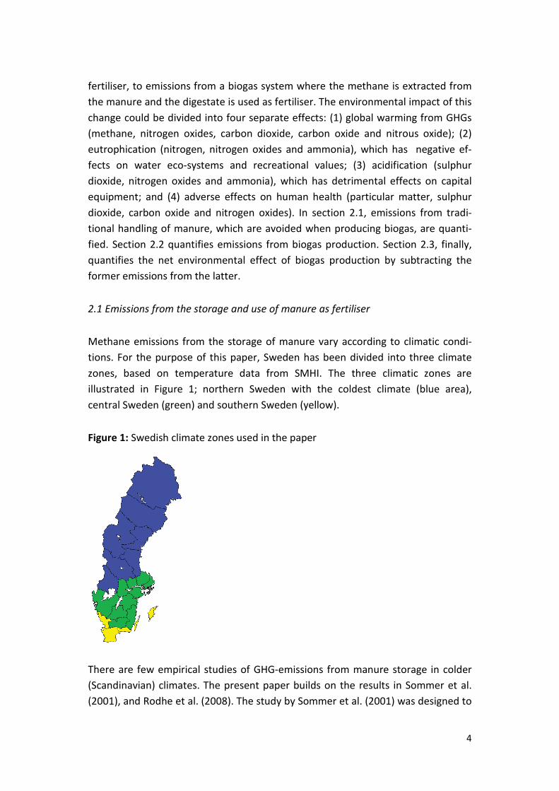
Methane emissions from the storage of manure vary according to climatic condi-tions. For the purpose of this paper, Sweden has been divided into three climate zones, based on temperature data from SMHI. The three climatic zones are illustrated in Figure 1; northern Sweden with the coldest climate (blue area), central Sweden (green) and southern Sweden (yellow).

Figure 1: Swedish climate zones used in the paper

There are few empirical studies of GHG-emissions from manure storage in colder (Scandinavian) climates. The present paper builds on the results in Sommer et al. (2001), and Rodhe et al. (2008). The study by Sommer et al. (2001) was designed to

5

mimic the conditions under which a typical Danish swine- or cattle farm operates, while the study by Rodhe et al. (2008) was a field experiment conducted near Uppsala and designed to represent the conditions on a Swedish cattle farm. Still, it should be kept in mind that whether or not the results can be generalized is subject to uncertainties (depending on, for instance, differences in the content of dry mat-ter (TS) and volatile solids (VS) in the slurry).

The differences in location, i.e. Denmark vs. central Sweden, are of significance as emissions increase with higher temperatures (IPCC, 2006). First, except in the southern part of Sweden, mean out-door temperatures are lower than in Denmark (cf. www.smhi.se). Second, in Sweden, slurry is typically transferred from the stable to the storage tank on a daily basis (communication with Maria Berglund, Hushållningssällskapet Halland) while, in the study by Sommer et al. (2001), it was assumed that swine slurry was transferred to the storage tank twice a month and cattle slurry once a month. As temperatures are higher in the stable, total emis-sions will be larger the longer the transfer is delayed. In addition, in Sweden, ma-nure is distributed on the lands twice a year (spring and autumn, cf. Rodhe et al., 2008) while in Sommer et al. (2001) it was assumed that manure was distributed in spring only. According to Sommer et al, distributing manure also in the autumn would reduce methane emissions by about 10 percent.

Thus, to adjust for effects of differences in storage practice between Denmark and Sweden, emissions occurring before the slurry is transferred to the storage tank, reported in Sommer et al. (2001), are ignored while emissions from the storage tank are multiplied by the factors 1.04, for swine slurry, and 1.08 for cattle slurry.1 Then, to adjust for effects of differences between Denmark and Sweden in the frequency of distributing manure on agricultural lands, emissions are reduced by a further 10 percent. The results are assumed to be representative for emissions of methane that would occur in the southern part of Sweden and presented in the “south” column in Table 2.1 below.

The results in Rodhe et al. (2008) are assumed to be representative for central Sweden and presented in the “central” column of Table 2.1. Emissions are likely to be even lower in northern Sweden but we have been unable to find estimates for that part of the country. In addition, the majority of farm animals are found in southern and central Sweden (cf. SCB, 2010).

1 Since the emissions are calculated on an annual basis and direct transfer would increase the aver-age time in the storage tank by 0.5/12 months for swine slurry, and 1/12 months for cattle slurry.

6

Table 2.1: Methane (CH4) emissions from manure storage in Sweden. Region South Central g methane / ton slurry from: Swine Cattle

2 213a 1 255a

N.a. 376b

Nm3 methane / ton slurry fromc Swine Cattle

16 Nm3 14 Nm3

16 Nm3 14 Nm3

g methane / Nm3 methane produced from Swine slurry Cattle slurry

138.313 89.643

N.a.

26.857 g CO2-equivalents / Nm3 methane produced fromd Swine slurry Cattle slurry

3 457.813 2 241.071

N.a.

671.429 Notes: a) Own calculations using the results in Sommer et al. (2001) and assuming that VS constitutes 64 kg/ton swine or cattle

slurry. b) Using the expression in Rodhe et al: (g CH4/ton slurry) = (VS x TS x 4.4g CH4-C/kg VS x 4/3 x 1000) and assuming that VS

is 80 % of TS, that TS is 8 % of the slurry and that 1 g CH4 = 1.33 g CH4-C. c) It is assumed that each ton of slurry contains 80 kg TS (8 %), and that 1 kg TS in swine (cattle) slurry produces 0.2 (0.175)

Nm3 CH4, (Berglund and Börjesson, 2003; Linné et al., 2008). d) GWP100 conversion factor: 1 g CH4 = 25 g CO2-equivalents

Table 2.1 shows how methane emissions from 1 ton of manure are translated into emissions measured in CO2-equivalents per Nm3 methane produced. For example, in the south of Sweden, 1 ton of swine slurry stored would result in 2 213 gram of methane emissions. As 1 ton of swine slurry produces biogas equivalent to 16 Nm3 methane, emissions per Nm3 methane would be 138.313 gram methane which, in turn, corresponds to 3 457.813 gram of CO2-equivalents per Nm3 methane.

Next, distributing manure on agricultural lands causes emissions of ammonia (NH3) and nitrous oxide (N2O). Table 2.2 shows results based on the study by Sommer et al. (2001). It is assumed that NH3-emissions correspond to about 5 percent of the ammonium content in the slurry, that the nitrate content is 5.1 (3.9) percent of the dry matter in swine- (cattle) slurry, and that the dry matter content in the slurry is 8 percent. It is assumed that the emissions in Sommer et al. (2001) are representative for what could be expected also in the colder Swedish climate.2 Ammonia does not contribute to the greenhouse effect. However, it contributes to eutrophication and acidification. The eutrophication potential (EP) is measured in phosphate equivalents (PO4-Eq.) and the acidification potential (AP) is measured in sulfur dioxide equivalents (SO2-Eq.).3

2 Rodhe et al (2008) contains no estimates of NH3 and N2O emissions from the distribution of slurry. According to Sommer et al. (2001), lower temperatures are expected to reduce the microbial activity generating emissions of nitrous oxide but it is not possible to quantify by how much. 3 See Lindahl et al., (2002) for the EPs and APs of different substances emitted.

7

Table 2.2: Emissions of nitrous oxide (N2O) and ammonia (NH3) from manure distrib-uted on agricultural lands in Sweden.

Emission g/ton slurry g CO2-Eq./Nm3 CH4 g PO4-Eq/ Nm3 CH4 g SO2-Eq/ Nm3 CH4 N2O from: Swine Cattle

43.91 33.53

817.821 713.710

NH3 from: Swine Cattle

250.00 264.77

5.469 6.619

29.688 35.331

Notes: 1 ton of swine (cattle) slurry assumed to contain 16 (14) MJ of raw energy. GWP100 conversion factor: 1 g N2O = 298 g CO2-equivalents EP conversion factor: 1 g NH3 = 0.35 g PO4-equivalents AP conversion factor: 1 g NH3 = 1.9 g SO2-equivalents

Adding, respectively, the CO2-, PO4- and SO2-equivalents in Tables 2.1 and 2.2 gives the total emission from storing and using manure as fertiliser.

Table 2.3: Total emissions/leakage from storing and using manure as fertiliser Emission g CO2-Eq./Nm3 CH4 g PO4-Eq/ Nm3 CH4 g SO2-Eq/ Nm3 CH4 Sum g CO2-Eq. Swine slurry: Cattle slurry:

South 4 275.634 2 954.781

Central 1 855.165 1 385.139

Ammonia from: Swine slurry Cattle slurry

5.469 6.619

29.688 35.331

Note: When calculating total emissions of CH4/Nm3, it is assumed that the lower temperatures in central Sweden reduce CH4-emissions from storage of swine slurry by the same percentage as they reduce CH4-emissions from storage of cattle slurry (i.e. by 70 %, cf. Table 2.1)

2.2 Emissions from biogas production and the use of digestate as fertiliser

Emissions from biogas production arise from the use of energy for transports and running the digestion facility. As the majority of Swedish farms produce only lim-ited amounts of manure, it is assumed that biogas is produced at a central facility to which manure is transported from several individual farms. Hence, emissions are caused by the use of energy when (1) transporting manure to the digestion facility, (2) transporting the digestate back to the farm and distributing it on the lands, and (3) running the digestion facility (i.e., it is assumed that there are no leakage of biogas from the digestion facility). These emissions (based on Börjesson and Berglund, 2003) are summarised in Table 2.4 below (for further details see Tables A1 – A3 in the Appendix).4

4 A farm running its own biogas facility avoids emissions from transporting manure to the facility and digestate back to the farm (Table A4 in Appendix A). This reduces emissions in Table 2.4 by about 20 percent per Nm3 methane produced.

8

Table 2.4: Emissions caused by energy used for transports of manure, and running the digestion facility.

Emission g/Nm3 CH4 g CO2-Eq./Nm3 CH4 g PO4-Eq/ Nm3 CH4 g SO2-Eq/ Nm3 CH4

Swine slurry

Cattle slurry

Swine slurry

Cattle slurry

Swine slurry

Cattle slurry

Swine slurry

Cattle slurry

CO2 516.250 590.00 516.250 590.00

CO 0.502 0.574 1.506 1.721

NOx 3.725 4.257 26.075 29.800 0.484 0.553 2.608 2.980

HC 0.259 0.296 2.846 3.253

CH4 0.069 0.077 1.719 1.964

SO2 < 0.000 < 0.000 < 0.000 < 0.000

PM2.5 0.069 0.077

Sum g CO2-Eq./Nm3 methane 548.396 626.738

Sum g PO4-Eq./Nm3 methane 0.484 0.553

Sum g SO2-Eq./Nm3 methane 2.608 2.980 Energy input MJ/Nm3 methane produced from: Swine slurry 12.188 Cattle slurry 13.929 GWP100 conversion factors: 1 g CO = 3 g CO2-Eq.; 1 g NOx = 7 g CO2-Eq.; 1 g HC = 11 g CO2-Eq.; and 1 g CH4 = 25 g CO2-Eq. EP conversion factor: 1 g NOx = 0.13 g PO4-Eq. AP conversion factor: 1 g NOx = 0.70 g SO2-Eq.

The energy required per ton manure is assumed to be the same regardless of what type of slurry that is processed and where it is processed. However, as methane production per ton manure is higher for swine- than for cattle slurry (cf. Table 2.1), emissions per Nm3 methane differ between types of slurry. It is assumed that slurry is transported to the central digestion facility by lorry, that the digestate is transported back to the farms by lorry and distributed on the lands by tractor (generating emissions of carbon oxide (CO), carbon dioxide (CO2), nitrogen oxides (NOx), hydrocarbon (HC), sulfur dioxide (SO2), and particular matter (PM2.5) from the combustion of diesel). In addition to contributing to the greenhouse effect, NOx also contribute to eutrophication and acidification. The distance from the farm to the digestion facility is assumed to be 10 km. The energy used for running the digestion facility is assumed to come from electric power (38 percent) and biogas (62 percent). The electricity is assumed to be produced from natural gas.5

5 According to Börjesson and Berglund (2003), emissions from electricity generated by natural gas are representative for the Swedish electricity production (a mix of mainly hydroelectric- and nuclear power and a small quantity from fossil fuels). It could be argued that emissions from the digestion facility should, instead, be elicited from those caused by a marginal increase in electricity produc-tion. As Sweden is fully integrated in the Nordic electricity market, this would mean coal-condensing power and result in substantially larger emissions (Uppenberg et al., 2001). The reason is that, even if biogas producers might use hydroelectric- or nuclear power, this would force other users to buy electricity produced by more polluting methods. However, in the long run, increased demand for

9

Distribution of digestate on agricultural lands causes emissions of nitrous oxide (N2O) and ammonia (NH3). Emissions of N2O contribute to global warming while emissions of NH3 contribute to eutrophication and acidification. On the other hand, the digestion process raises the concentrate of ammonium nitrate which is more accessible to plants. Thus, substituting manure with digestate may reduce nitrogen leakage by about 20 percent (or 250 g N) per ton manure (Börjesson and Berglund, 2003). This would partly counteract the contribution to eutrophication from the in-crease in ammonia emissions when distributing digestate instead of slurry. To esti-mate the net effect, the nitrogen and ammonia leakages are converted to phosphor (PO4) equivalents. Results are presented in Table 2.5.

Table 2.5: Emissions and leakage when replacing manure with digestate. Emission g/ton manure g CO2-Eq./

Nm3 CH4 g PO4-Eq/ Nm3 CH4

g SO2-Eq/ Nm3 CH4

N2O from distribution ofa digestate from swine slurry: digestate cattle slurry:

26.35 22.16

490.800 471.771

NH3 from distribution ofa digestate from swine slurry: digestate from cattle slurry:

301.32 322.40

6.592 8.060

35.782 43.754

Reduced N-leakage due to better uptake ofb digestate from swine slurry: digestate from cattle slurry:

-250.00 (-304.878) -250.00 (-304.878)

-6.669 -7.622

Net effect on nutrient emis-sion/leakage by using dige-state from swine slurry: cattle slurry:

-0.077 0.438

Notes: a) Based on Sommer et al. (2001)

b) Based on Börjesson and Berglund (2003), converted to NH3-equivalents (in parentheses) by dividing g N/ton slurry by 0.82 (communication with Maria Berglund, Hushållningssällskapet, Halland).

GWP100 conversion factor: 1 g N2O = 298 g CO2-equivalents EP conversion factor: 1 g NH3 = 0.35 g PO4 AP conversion factor: 1 g NH3 = 1.9 g SO2

Finally, the digestate may also substitute for inorganic fertiliser, implying that de-mand for, and emissions from the production of inorganic nitrogen, will be re-duced.6 Table 2.6 presents estimates of reductions in emissions from the produc-tion of inorganic fertiliser when it is substituted by digestate. It is assumed that 1 ton of manure results in 1 ton of digestate which replaces 220 g of inorganic ferti-liser (Börjesson and Berglund, 2003). To convert this to reduction per Nm3 methane electricity may change the production mix in the Nordic market and reduce emissions from marginal electricity. We have, therefore, chosen to keep the assumptions in Börjesson and Berglund (2003). 6 Table A5 in the Appendix presents estimates of life-cycle emissions per kg nitrogen in the production of inorganic N-fertiliser from Davis and Haglund (1999).

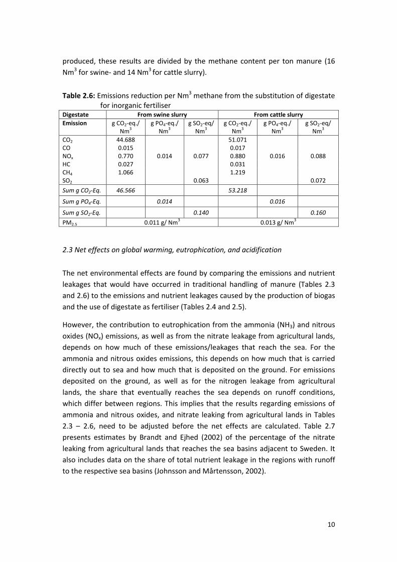
10

produced, these results are divided by the methane content per ton manure (16 Nm3 for swine- and 14 Nm3 for cattle slurry).

Table 2.6: Emissions reduction per Nm3 methane from the substitution of digestate for inorganic fertiliser

Digestate From swine slurry From cattle slurry Emission g CO2-eq./

Nm3 g PO4-eq./

Nm3 g SO2-eq/

Nm3 g CO2-eq./

Nm3 g PO4-eq./

Nm3 g SO2-eq/

Nm3 CO2 44.688 51.071 CO 0.015 0.017 NOx 0.770 0.014 0.077 0.880 0.016 0.088 HC 0.027 0.031 CH4 1.066 1.219 SO2 0.063 0.072 Sum g CO2-Eq. 46.566 53.218

Sum g PO4-Eq. 0.014 0.016

Sum g SO2-Eq. 0.140 0.160 PM2.5 0.011 g/ Nm3 0.013 g/ Nm3

2.3 Net effects on global warming, eutrophication, and acidification

The net environmental effects are found by comparing the emissions and nutrient leakages that would have occurred in traditional handling of manure (Tables 2.3 and 2.6) to the emissions and nutrient leakages caused by the production of biogas and the use of digestate as fertiliser (Tables 2.4 and 2.5).

However, the contribution to eutrophication from the ammonia (NH3) and nitrous oxides (NOx) emissions, as well as from the nitrate leakage from agricultural lands, depends on how much of these emissions/leakages that reach the sea. For the ammonia and nitrous oxides emissions, this depends on how much that is carried directly out to sea and how much that is deposited on the ground. For emissions deposited on the ground, as well as for the nitrogen leakage from agricultural lands, the share that eventually reaches the sea depends on runoff conditions, which differ between regions. This implies that the results regarding emissions of ammonia and nitrous oxides, and nitrate leaking from agricultural lands in Tables 2.3 – 2.6, need to be adjusted before the net effects are calculated. Table 2.7 presents estimates by Brandt and Ejhed (2002) of the percentage of the nitrate leaking from agricultural lands that reaches the sea basins adjacent to Sweden. It also includes data on the share of total nutrient leakage in the regions with runoff to the respective sea basins (Johnsson and Mårtensson, 2002).

11

Table 2.7: Percentage of nutrient leakages from agricultural lands reaching the sea Sea basin Share of leakage reaching the seaa Share of total leakageb Gulf of Bothnia – northern part 67 2.9 Gulf of Bothnia – southern part 69 4.8 Baltic sea 59 38.0 Öresund 70 17.2 Kattegat 66 14.1 Skagerrak 70 23.3 Notes: a) Data from Brandt and Ejhed (2002).

b) Data from Johnsson and Mårtensson (2002)

Biogas produced in the south of Sweden affect eutrophication of the Baltic, the Öresund and the Kattegat. The average share of nutrients leaking from agricultural lands in this part of the country that reaches the sea (using the share of total leakage to each sea basin as weights) is about 65 percent. Biogas produced in central Sweden affect eutrophication of the Baltic and the Skagerrak. The average share of nutrients leaking from agricultural lands in this part of the country that reaches the sea is about 63 percent. As the difference is small, the reduction in nutrient leakage is multiplied by 0.64 (i.e. the mean of these two averages) regardless of where the biogas has been produced.

To our knowledge, there are no estimates of how much of the Swedish ammonia and nitrous oxides emissions that is carried directly out to sea. To avoid over-estimating their effects on eutrophication, it is assumed that all of them are depos-ited on the ground. Thus, all emissions/leakages of phosphate-equivalents in Tables 2.3 – 2.6 are adjusted in this way.

In a similar vein, the contribution to acidification depends on how much of the ammonia, the nitrous oxides and the sulphur dioxide (SO2) emissions that are de-posited on the ground in Sweden. As it has been assumed that all of the ammonia- and nitrous oxides emissions are deposited on the ground, the question primarily concerns the sulphur dioxide emissions. According to Statistics Sweden (SCB, 2000), about 29 percent of the total Swedish sulfur emissions are deposited in Sweden.7 Thus, to estimate the contribution to acidification, the sulphur dioxide equivalents from emissions of ammonia and nitrous oxides in tables 2.3 – 2.6 have not been adjusted while those caused by emissions of SO2 have been multiplied by the factor 0.29. Table 2.8, below, shows the net effects on emissions when substituting

7 It may be argued that SO2-emissions “exported” from Sweden also should be included as they have adverse environmental effects in other countries. However, estimates of these effects are scarce and uncertain as the SO2-molecules react chemically with other air molecules and form new sub-stances with different environmental effects. The extent of such reactions depends on atmospheric conditions and is difficult to estimate. Therefore, only those effects that affect Sweden are ac-counted for, implying that the damage caused by the SO2-emissions probably are under-estimated.

12

traditional handling of manure with biogas production after all these adjustments have been done.

Table 2.8: Net effects on emissions from biogas production (per Nm3 methane) South of Sweden Central part of Sweden Biogas produced from

Swine slurry Cattle slurry Swine slurry Cattle slurry

Sum g CO2-Eq./Nm3

(Greenhouse gases) -3 283.004

(-3 392.696) -1.909.490

(-2 039.603) -869.187

(-876.401) -339.848

(-345.965) Sum g PO4-Eq./Nm3

(Eutrophication) -3.249

(- 3.314) -3.612

(-3.684) -3.249

(- 3.314) -3.612

(-3.684) Sum g SO2-Eq./Nm3

(Acidification) +8.607

(+8.091) +11.294

(+10.729) +8.607

(+8.091) +11.294

(+10.729) Sum PM2.5 g/Nm3 +0.058

(+0.049) +0.064

(+0.054) +0.058

(+0.049) +0.064

(+0.054) Notes: A negative sign indicates that emissions are reduced by X g/Nm3 methane produced while a positive sign implies that

emissions increase by X g/ Nm3 biogas produced. Results for a farm running its own digestion facility in parentheses.

As evident from table 2.8, the net effect on GHG-emissions is highly dependent on where the biogas is produced and, to a lesser extent, on what kind of manure that is used. Nevertheless, producing biogas from swine or cattle slurry and replacing slurry and inorganic fertiliser with digestate, reduce emissions of GHGs and substances contributing to eutrophication. On the other hand, emissions of sub-stances contributing to acidification, and of particular matter, all increase.

3. The societal value of biogas production

The impact of biogas production from manure on the environment is twofold. First, it has the potential to reduce emissions of GHGs and nitrogen leakage which is a positive external effect. Second, emissions of particular matter and acidifying sub-stances may increase, thus, causing a negative externality. The positive and nega-tive environmental effects are expressed in different units (i.e. CO2-, PO4-, SO2-equivalents, and PM) in Table 2.8. Thus, in order to be comparable and allow an evaluation of the total impact, they have to be measured in value terms. The usual way to convert units to values is to use their market prices. However, being exter-nalities, there are no natural market prices on emissions of GHGs, substances con-tributing to eutrophication and/or acidification, or PM. When there are no market prices, values may be elicited by investigating peoples’ willingness to pay (WTP) for a good (or avoiding a hazard) by indirect methods, so called contingent valuation (cf. Alberini and Kahn, 2006). However, relying on peoples’ WTP for avoiding global

13

warming for eliciting the value of a reduction in GHG-emissions may be problem-atic as the full effects on global warming of GHG-emissions will not be realised by the present generation. This has prompted discussions on the ethical implications of basing decisions on the present generation’s valuations (cf. Stern, 2007) and, it has been suggested that, rather than using the WTP of the present generation which, inter alia, is affected by their appreciation of the problem and by their time-preferences, the value of reduced GHG-emissions should be elicited differently. In addition, the impact of GHG-emissions is global while effects of, for example, par-ticular matter are local. Thus the emissions of GHGs will have an impact both on Sweden and other countries while emissions of particular matter only will affect the environment in Sweden. This further complicates the problem of using peoples’ WTP to value reductions in GHG-emissions as WTP will also depend on incomes which differ substantially between countries.

Contrary, the effects of emissions of eutrophicating and acidifying substances, as well as of particular matter are local and their impacts are realised by the present generation. Hence, the above arguments against using the WTP of the present generation to elicit the value of a reduction in emissions of substances contributing to eutrophication, or the costs of an increase in emissions of acidifying substances and particular matter, do not apply.

Regarding GHG-emissions, several attempts to estimate the value of the damages caused have been made. The results differ depending on the underlying assump-tions and the method used as discussed in section 3.1. Fewer studies have at-tempted to estimate the value of the marginal damage caused by the other emis-sions. The problems of valuing these effects are discussed in sections 3.2 and 3.3. Finally, the total subsidy is calculated in section 3.4 by adding the values of the re-duction in GHG-emissions and eutrophicating substances and subtracting the costs of increased emissions of PM2.5 and acidifying substances.

3.1 The value of reduced GHG-emissions

Though the full environmental impact of GHG-emissions is not known, it is widely recognized that there is a link between GHG-emissions and a rising global tempera-ture. This implies that GHGs cause damage to the environment resulting in a cost for society. To limit these emissions at an efficient level there should be a cost at-tached to them. From a theoretical point of view, this cost/price should equalize the marginal damage cost and marginal abatement cost for these emissions. Fur-thermore, to achieve an efficient reduction, this price should be the same for all sources of emissions on a global basis. In practice however, it is difficult to correctly

14

asses the marginal damage cost and marginal abatement cost of GHG-emissions and it is unlikely that a political agreement on a price mechanism can be reached at the global level. As a global price does not exist and, as there is no consensus on the correct value of emission reductions among researchers, one will have to use indirect methods to attach a value to reductions of GHG-emissions. Possible alter-natives are; (1) an estimation of the marginal abatement cost to reach a given level of emission reduction, (2) use the current costs of GHG-emissions in regional sys-tems such as the EU Emission Trading System (EU-ETS); (3) use national taxes as an indicator for the value attached to emission reductions in a nation.

The abatement cost will depend on the emission reduction target. A more ambi-tious target will imply higher abatement costs since the least costly measures (per unit of emission reduction) could be expected to be implemented before more ex-pensive ones. Even though technological progress may reduce the costs of particu-lar measures in the future it is likely that more expensive abatement measures will have to be implemented to meet the climate target as the amount of emissions is reduced further. The value of current emission reductions in the agricultural sector should be based on the value of current reductions and not on possible future val-ues of emission reductions (e.g. estimated future abatement costs). A policy that values emission reductions based on their possible future values would be ineffi-cient as it would support more costly measures to reduce GHG-emissions by a given amount. If the value of emission reductions increases in the future, the policy should be revised to take that into account. In addition, the value of emission re-ductions required to reach the 2 Co target sometime in the future is highly uncer-tain, and Sweden will not be able to reach the climate targets by itself; hence the alternative of using abatement costs as basis for the price of GHG-emissions seems less relevant for assessing the value of current reductions in the agricultural sector.

The price in the EU-ETS reflects the value of GHG-reductions in sectors included in the trading system. It could be discussed whether this is a reasonable price given the reduction targets of the EU but that is not within the scope of this paper. How-ever, the Swedish policy makers could choose to buy emission permits in the EU-ETS to force a reduction in emissions from firms in the EU-ETS at the market price of emission permits. Hence, if measures in the agricultural sector are more expen-sive than buying emission permits, it is more cost-effective to buy emission per-mits. It should be noted that the price of emission permits fluctuates over time and that purchases of permits would increase their price since the number of emission permits is limited. The extent of the price effect will depend on the abatement cost of firms in the EU-ETS and the amount of permits purchased. Thus, it is actually difficult to know the exact cost of a given emission reduction obtained by pur-

15

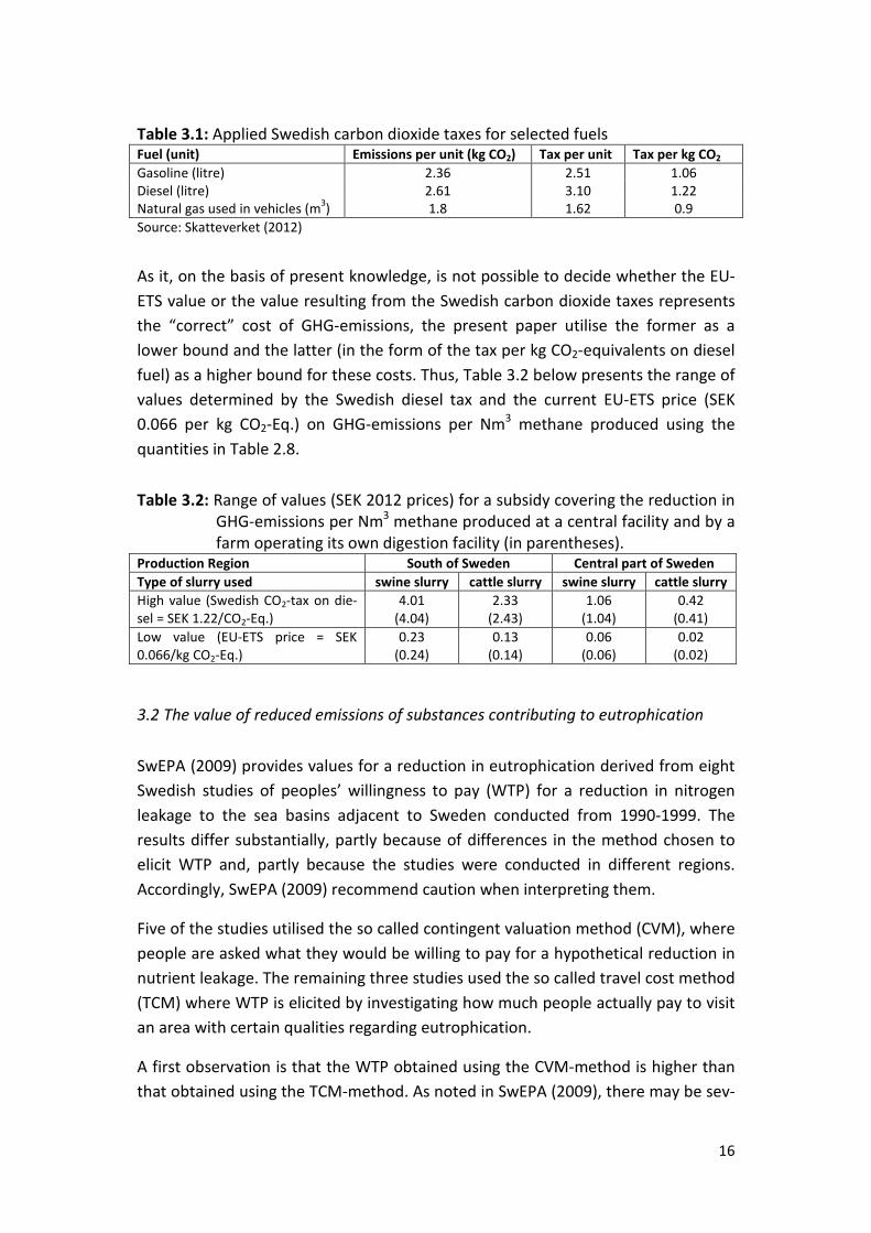
chases of emission permits. The current (February 13, 2012) price of EU allowances is € 7.5 (ICE 2012) or SEK 66.4 per ton CO2-equivalents.8 This price is low relative to recent prices. During 2009, for example, the price never fell below € 8 and it was as high as € 15.6 per ton CO2-equivalents, with prices above € 13 for a substantial part of the year (European Climate Exchange 2010). Moreover, the prices for emission permits could be expected to increase over the next few years as the number of permits is to be reduced and economic growth improves, thus increasing the de-mand for emission permit. Calculating the value of reductions of GHG-emissions based on the current price of permits in the EU-ETS should thus be considered a lower bound for the value of GHG-emission reductions in the agricultural sector.

Emission taxes could be said to reflect the value policy makers attach to reductions of GHG-emissions. These values could of course differ across sectors and countries so it is not straightforward to draw inferences on the true value attached to a re-duction. This paper uses Swedish taxes on carbon dioxide emissions as they reflect the value attached to a reduction of GHG-emissions in Sweden by Swedish policy makers. The same policy makers who would decide on measures to reduce GHG-emissions from the agricultural sector. However, it should be noted that the Swedish carbon dioxide taxes are high in an international perspective and will, thus stimulate abatement measures that are not efficient from a global perspective. For consistency, the value of reductions of carbon dioxide emissions from taxed sectors (for example transports) should equal the value of reductions of GHG-emissions in other sectors, e.g. the agricultural sector; hence the tax on carbon dioxide in the transport sector can be used to calculate the value of GHG-emission reductions in the agricultural sector from a national Swedish perspective. In practice, Swedish policy makers seem to value reductions of carbon dioxide emissions differently depending on the taxed object. This suggests that the tax is not a pure carbon tax implemented to reduce carbon dioxide emission but also used to achieve other policy objectives. As can be seen from Table 3.1 the carbon dioxide tax on fossil fuel in the transport sector varies from SEK 0.9 to SEK 1.22 per kg CO2. There is thus no consistent policy on taxation of carbon dioxide emissions even within the transport sector. The highest value is interpreted as the highest value attached to a reduction of GHG-emission in the transport sector since the tax is labelled as a car-bon dioxide tax even though it is possible that other policy concerns are also reflected by the tax.

8 The exchange rate in January 2012 was € 1 = SEK 8.8464 (www.riksbanken.se)

16

Table 3.1: Applied Swedish carbon dioxide taxes for selected fuels Fuel (unit) Emissions per unit (kg CO2) Tax per unit Tax per kg CO2

Gasoline (litre) 2.36 2.51 1.06 Diesel (litre) 2.61 3.10 1.22 Natural gas used in vehicles (m3) 1.8 1.62 0.9 Source: Skatteverket (2012)

As it, on the basis of present knowledge, is not possible to decide whether the EU-ETS value or the value resulting from the Swedish carbon dioxide taxes represents the “correct” cost of GHG-emissions, the present paper utilise the former as a lower bound and the latter (in the form of the tax per kg CO2-equivalents on diesel fuel) as a higher bound for these costs. Thus, Table 3.2 below presents the range of values determined by the Swedish diesel tax and the current EU-ETS price (SEK 0.066 per kg CO2-Eq.) on GHG-emissions per Nm3 methane produced using the quantities in Table 2.8.

Table 3.2: Range of values (SEK 2012 prices) for a subsidy covering the reduction in GHG-emissions per Nm3 methane produced at a central facility and by a farm operating its own digestion facility (in parentheses).

Production Region South of Sweden Central part of Sweden Type of slurry used swine slurry cattle slurry swine slurry cattle slurry High value (Swedish CO2-tax on die-sel = SEK 1.22/CO2-Eq.)

4.01 (4.04)

2.33 (2.43)

1.06 (1.04)

0.42 (0.41)

Low value (EU-ETS price = SEK 0.066/kg CO2-Eq.)

0.23 (0.24)

0.13 (0.14)

0.06 (0.06)

0.02 (0.02)

3.2 The value of reduced emissions of substances contributing to eutrophication

SwEPA (2009) provides values for a reduction in eutrophication derived from eight Swedish studies of peoples’ willingness to pay (WTP) for a reduction in nitrogen leakage to the sea basins adjacent to Sweden conducted from 1990-1999. The results differ substantially, partly because of differences in the method chosen to elicit WTP and, partly because the studies were conducted in different regions. Accordingly, SwEPA (2009) recommend caution when interpreting them.

Five of the studies utilised the so called contingent valuation method (CVM), where people are asked what they would be willing to pay for a hypothetical reduction in nutrient leakage. The remaining three studies used the so called travel cost method (TCM) where WTP is elicited by investigating how much people actually pay to visit an area with certain qualities regarding eutrophication.

A first observation is that the WTP obtained using the CVM-method is higher than that obtained using the TCM-method. As noted in SwEPA (2009), there may be sev-

17

eral reasons for this. For instance, as the TCM-method elicits WTP by investigating the travel costs for people who actually have visited the area, it only includes the effect of eutrophication on the value of the area for users (so called utilisation-values). By asking people for their WTP regardless of if they have visited the area or not, the CVM-method also allows the inclusion of the effect of eutrophication on the value of the area for non-users (non-utilisation values). Everything else equal, this could lead to higher WTP in studies using the CVM-method without casting doubt on the results. On the other hand, since the CVM-method asks people to state their WTP, there is a hypothetical element involved, which has been shown to lead to upward bias in the results. Meta-studies suggest that this upward bias results in that the elicited WTP, on average, is about three times higher than what people actually would be willing to pay for the good in the market if they were given the opportunity to do so (List and Gallet, 2001; Murphy et al., 2005; Svensson, 2009). Consequently, in SwEPA (2009) the results from the studies using the CVM-method have been divided by the factor 3 to adjust for this problem.

A second observation is that the underlying studies are at least 12 years old. Hence, in SwEPA (2009) the results have been adjusted for changes in prices and incomes that have occurred since they were undertaken to express WTP in 2006 prices. However, these adjustments do not account for changes in peoples’ views on the significance of the eutrophication problem that might have occurred. As there has been much discussion of the effects of eutrophication since 1999 which, inter alia, has led to the adoption of the Baltic Sea Action Plan in November 2007, it might be conjectured that peoples’ concerns for the effects of eutrophication have increased during the period. In that case, the WTP elicited from these early studies are likely to under-estimate the value of reductions in eutrophicating substances.

A third observation is that the original question asked in the CVM-studies was what the respondents would be willing to pay for a “large” reduction in nitrogen leakage. In SwEPA (2009), this was interpreted as how much the respondents would be willing to pay for a 50 percent reduction in nitrogen supplied to the sea basins in question (i.e. a reduction of about 2 556 tonnes annually). This was recalculated to WTP for a reduction of one kg nitrogen by simply dividing the WTP for the 50 percent reduction by 2 556 000. The result is then interpreted as a proxy for the WTP for a marginal reduction in nitrogen leakage. Now, if the marginal utility of reducing eutrophication is decreasing, it would be expected that the value of the first kg of reduced leakage is larger than that of the last. In that case, the values elicited from the underlying studies may under-estimate the value of a marginal reduction in nitrogen leakage. However, this may be a smaller problem in the

18

present case since production of biogas from manure, if undertaken by several farmers, would result in non-marginal reductions in nutrient leakage.

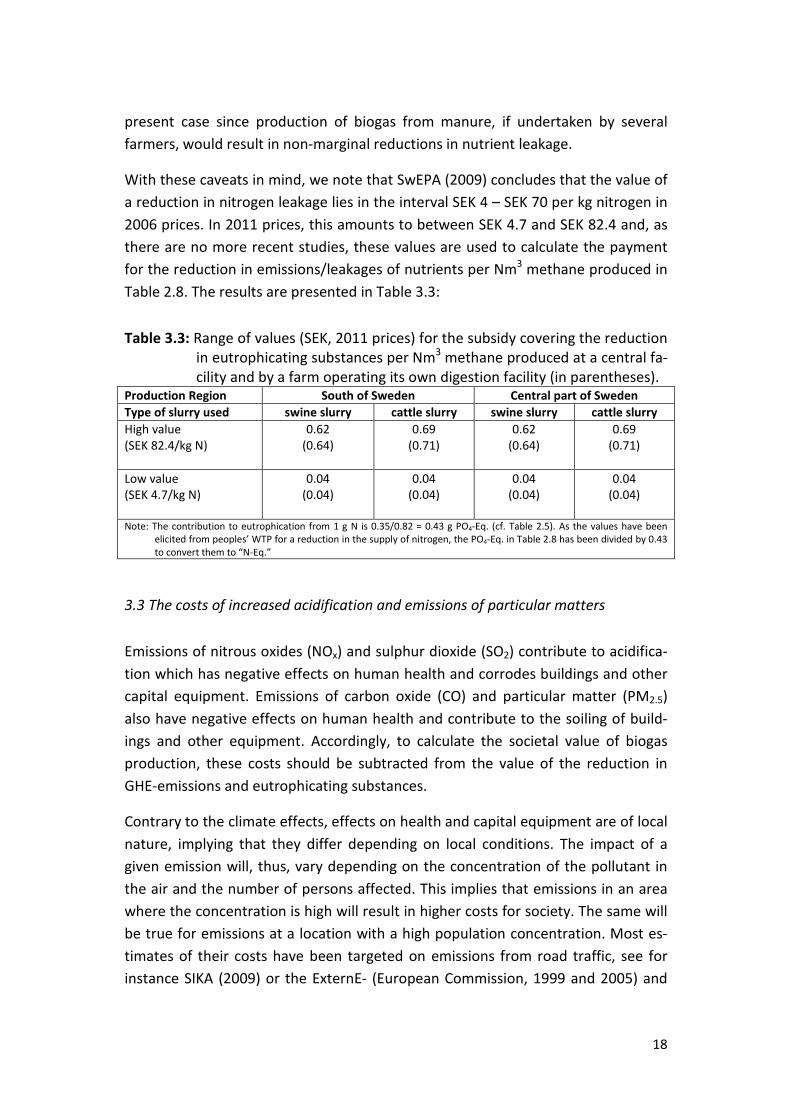
With these caveats in mind, we note that SwEPA (2009) concludes that the value of a reduction in nitrogen leakage lies in the interval SEK 4 – SEK 70 per kg nitrogen in 2006 prices. In 2011 prices, this amounts to between SEK 4.7 and SEK 82.4 and, as there are no more recent studies, these values are used to calculate the payment for the reduction in emissions/leakages of nutrients per Nm3 methane produced in Table 2.8. The results are presented in Table 3.3:

Table 3.3: Range of values (SEK, 2011 prices) for the subsidy covering the reduction in eutrophicating substances per Nm3 methane produced at a central fa-cility and by a farm operating its own digestion facility (in parentheses).

Production Region South of Sweden Central part of Sweden Type of slurry used swine slurry cattle slurry swine slurry cattle slurry High value (SEK 82.4/kg N)

0.62 (0.64)

0.69 (0.71)

0.62 (0.64)

0.69 (0.71)

Low value (SEK 4.7/kg N)

0.04 (0.04)

0.04 (0.04)

0.04 (0.04)

0.04 (0.04)

Note: The contribution to eutrophication from 1 g N is 0.35/0.82 = 0.43 g PO4-Eq. (cf. Table 2.5). As the values have been elicited from peoples’ WTP for a reduction in the supply of nitrogen, the PO4-Eq. in Table 2.8 has been divided by 0.43 to convert them to “N-Eq.”

3.3 The costs of increased acidification and emissions of particular matters

Emissions of nitrous oxides (NOx) and sulphur dioxide (SO2) contribute to acidifica-tion which has negative effects on human health and corrodes buildings and other capital equipment. Emissions of carbon oxide (CO) and particular matter (PM2.5) also have negative effects on human health and contribute to the soiling of build-ings and other equipment. Accordingly, to calculate the societal value of biogas production, these costs should be subtracted from the value of the reduction in GHE-emissions and eutrophicating substances.

Contrary to the climate effects, effects on health and capital equipment are of local nature, implying that they differ depending on local conditions. The impact of a given emission will, thus, vary depending on the concentration of the pollutant in the air and the number of persons affected. This implies that emissions in an area where the concentration is high will result in higher costs for society. The same will be true for emissions at a location with a high population concentration. Most es-timates of their costs have been targeted on emissions from road traffic, see for instance SIKA (2009) or the ExternE- (European Commission, 1999 and 2005) and

19

HEATCO-projects (Bickel et al., 2006). This seems as a relevant starting point also in the present case.

In SIKA (2009), it is suggested that the values to be used for societal cost-benefit analysis in Sweden may be derived using the following expression based on esti-mates by Leksell (1999 and 2000):

( ) CUEPopFemission KgCost

iv ×××= 5.0029.0 (1)

where Fv is the so called ventilation factor in region v, Popi is population size at location i, and CUE is cost per unit exposed.

The product of the first three terms – i.e. 0.029 × Fv × (Popi)0.5 – quantifies the number of persons exposed to a concentration of 1 µg/m3 annually per kg sub-stance emitted at a given location. This depends on population size and meteoro-logical and topological conditions at that location. Differences in meteorological and topological conditions are picked up by the ventilation factors which Leksell have recalculated from estimates by IVL (Persson et al., 1999; Persson and Sjöberg, 1999).9 However, precisely how this has been done is not transparent. One differ-ence between Leksell and IVL is the expression for the concentration) of a given substance (which also explains why the ventilation factor is multiplied by the square root of population rather than by population itself).10 Leksell also corrects the empirically measured concentrations at different locations for differences in heating requirements,11 presumably by replacing the average concentrations dur-ing the winter time (when demand for heating differs the most) used by IVL with the annual average concentrations, but the author is not clear on this. Finally, the multiplicative constant (i.e. 0.029) in eq. (1) was calculated from the expression for concentration level (θi = k × Fv × (Popi)0.5) using empirical data on θ and Pop from Södertälje (a municipality for which Fv = 1).

The last term in eq. (1) – CUE – is the value of the damage caused per person (or capital unit) exposed to 1 µg/m3 annually of the substance. This differs depending

9 Leksell’s ventilation factors ranges from 1 to 1.6 with the lowest values in the southern coastal regions and the highest values in the northern inland regions of Sweden (SIKA, 2009). 10 IVL, using empirical data on concentration levels (θ) during the winter 1997/1998 from 33 munici-palities, found that the function θ = Fv × Log(Popi) gave a reasonably good estimate of the concen-tration, implying that Fv = θ/Log(Popi). However, Leksell (2000) found that the expression θ = k × Fv × (Popi)

0.5 fitted the empirically measured θ’s better. This implies that, in Leksell, Fv = θ/[k × (Popi)0.5].

11 Other things equal, a higher demand for heating (due to colder climate) implies higher emission levels and a higher concentration of substances. However, as Fv is intended to account for dif-ferences in concentration caused by dispersion of a given level of emissions, differences in concen-tration caused by higher emission levels should not affect Fv.

20

on type of emissions but not between locations. Table 3.4 shows CUEs for the respective emissions based on estimates by Leksell and converted to 2006 prices by adjusting for changes in prices and incomes.

Table 3.4: Cost per unit exposed (CUE) by substance Substance CUE (SEK 2006) PM2.5 515 SO2 15.1 NOx 1.8 VOC 3.0 Source: SIKA, 2009 Notes: VOC stands for “Volatile Organic Compounds“ which includes CO as one substance.

The CUE for PM2.5 includes the value of negative health effects (mortality and morbidity) as well as the costs of soiling. The CUEs for SO2, NOx and VOC includes the value of negative health effects as well as the costs of capital deterioration caused by corrosion.

The CUE for PM2.5, is the product of the effects on, respectively, life-expectancy, morbidity and soiling, and the values of these effects, i.e.:

CUE = ΔLE × WTPLY + ΔI × WTPI + ΔS × WTPS (2)

where ΔLE is change in life-expectancy, WTPLY is willingness to pay for a life-year, ΔI is change in morbidity (illness), WTPI is willingness to pay for avoiding morbidity, ΔS is change in soiling, and WTPS is willingness to pay to avoid soiling.

As to mortality costs (ΔLE × WTPLY), Leksell utilised the results regarding the effect on age-specific mortality from a 1 µg/m3 increase in annual exposure to PM2.5 in Bellander et al. (1999).12 To estimate how this change in mortality affected life-expectancy, Leksell then used survival analysis, acknowledging that the quality of life-years may deteriorate with age as well as that future life-years (regardless of their quality) should be discounted,. Finally, WTP for a life-year was derived from the WTP for a statistical life (see Appendix B). This resulted in the following expression for the societal cost of mortality caused by an increase in exposure:

poptacc

pop

LYLE

LEVSLWTPLE

∆

∆×=×∆ exp (3)

where VSL is the value of a statistical life obtained from peoples’ WTP for reducing the risk of fatal traffic accidents, popLEexp∆ is the expected number of quality adjusted and discounted life-years lost

12 Using data from three American studies (Dockery et al., 1993; Pope et al., 1995; Abbey et al., 1999), Bellander et al. found that age-specific mortality rates would increase by about 0.57 percent. This has been confirmed in a later study (Pope et al., 2002) who estimated the effect on age specific mortality to be about 0.6 percent.

21

due to increased exposure in the population, and poptaccLE∆ is the expected number of quality ad-

justed and discounted life-years lost due to fatal traffic accidents in the population.

The morbidity costs (ΔI × WTPI) caused by increased exposure to PM2.5 was cal-culated as a percentage (24 percent) of the mortality costs on the grounds that existing estimates where uncertain and that the ratio of morbidity costs to the cost of mortality in other studies (e.g. ExternE) where about 24 percent. The origin of the soiling costs (ΔS × WTPS) is not explained. However, they amounted to about 17 percent of the sum of mortality and morbidity costs in the original 1999-values (Leksell, 2000).13

Leksell only discusses the derivation of the CUE for particular matter (PM2.5). As SIKA does not provide explanations for the derivation of any of the CUEs, values for nitrous oxides (NOx), sulphur dioxide (SO2) and VOC are very uncertain. According to some studies (Dockery et al., 1993; Pope et al., 1995 and 2002; Abbey et al., 1999; Krewski et al., 2000; Forsberg, 2002; Sunyer et al., 2003; Nerhagen et al., 2005), health effects of sulphur dioxide and nitrous oxides cannot be separated from those of particular matter as emissions are highly correlated. As the health effects of particular matter are considered more prominent than those of the other substances, it is suggested that health effects of the other two substances should be assumed included in those estimated for particular matter. In that case, the CUEs for SO2 and NOx in SIKA (2009) should be reduced by the amounts accounting for negative health effects in order to avoid double counting. However, these amounts are unknown.

Using the method suggested by SIKA (2009) and assuming that the biogas is pro-duced at a rural location in southern or central Sweden, the cost per kg emission in 2011 prices would be as shown in Table 3.5:

Table 3.5: Cost per kg emission in a rural location (SIKA values, 2011 prices). SEK/kg South of Sweden (Fv = 1)

Average population density = 12.0/km2 Central Sweden (Fv = 1.1) Average population density = 7.4/km2

PM2.5 2 158.08 1 864.17 SO2 63.28 54.66 NOx 7.54 6.52 CO 12.57 10.86 Note: In accordance with Leksell (2000), it is assumed that the area affected by the emissions is defined by a circle with a

radius of 20 km = 1256 km2 Data on average population densities from Statistics Sweden.

13 As the 2006-values are equal to the 1999-values multiplied by the changes in consumer prices and real GDP, the costs of reduced life-expectancy caused by PM2.5 are about SEK 355, the costs of morbidity about SEK 85, and the soiling costs about SEK 75 per person exposed, in 2006 prices.

22

Given the uncertainties in the SIKA-values, one may consider replacing the costs per kg emission with those estimated in the ExternE- and HEATCO-projects. ExternE and it successor HEATCO applied the same basic method as Leksell to derive the cost per kg emission (i.e. multiplying the number of people exposed to 1 µg/m3 of the substance by the cost per individual exposed). The quantification of health ef-fects (the effects on mortality and morbidity caused by increased exposure) also rest on the same American studies as SIKA/Leksell. The differences are that they use another model (the so called RoadPol-model, cf. Bickel et al., 1999) than SIKA/Leksell to estimate concentrations, and value health effects differently.

The problem with the RoadPol model is that, while it seems to give reasonably good approximations of the concentrations people are exposed to for Continental Europe, it has not been validated for Swedish climate conditions (cf. Nerhagen et al., 2003 and 2005). The Swedish climate differs from that of Continental Europe in that it, particularly during the winter, is more stable with a higher frequency of temperature inversions, implying a higher concentration of emitted substances in Sweden. As to the value of the health effects, the cost of reduced life-expectancy was elicited from peoples’ WTP for avoiding the loss of one life-year, while the cost of increased morbidity was estimated by combining cost-of-illness studies (quanti-fying direct medical costs and costs of absenteeism) with studies of peoples’ WTP for avoiding the loss of quality of life caused by morbidity (cf. European Commis-sion, 2005). It should be noted that the valuation of a life-year rests on results from one empirical study carried out in three countries only; the UK, Italy and France (cf. European Commission, 2005). Similarly, the costs of morbidity are based on cost-of-illness studies in seven EU-countries (Sweden not included). These costs, as well as WTP for avoiding the loss of quality of life, depend on the specific ailment and have only been estimated for a limited number of conditions.14

As to the costs of capital deterioration caused by soiling and acidification, the dam-ages caused by an increase in emissions are based on exposure-response functions for various building materials (cf. Bickel et al., 2006). Values of the damages are said to have been elicited from estimates of restoration costs using market prices in the respective countries. However, precisely how this has been done is not clear. A final caveat is that in Bickel et al. (2006) cost estimates from the HEATCO-project are presented as average costs for urban and rural areas, respectively, in each country. This implies that it is not possible to differentiate costs between rural

14 Respiratory illness requiring hospital admission, Respiratory illness requiring emergency room visit, Asthma and lower respiratory illness requiring consultation by a general practitioner, Chronic bronchitis, Days of restricted (major and minor) activity, Days of coughing (cf. European Commission (2005).

23

locations. Nevertheless, recalculating the HEATCO-values into 2011 SEK prices, would give the costs per kg emission presented in Table 3.6.:

Table 3.6: Cost for emission at a rural location in Sweden (HEATCO values, 2011 prices).

Emission SEK/kg Particular matter (PM2.5) 504.79 Sulphur dioxide (SO2) 12.62 Nitrous oxides (NOx) 16.41 Carbon oxide (CO) 3.79 Source Bickel et al. (2006). Note: The HETACO values were expressed in € in 2002 prices, have been recalculated to SEK 2011 prices by first using the

exchange rate in 2002 (€ 1 = SEK 9) and then multiplying by the change in CPI from 2002 to 2011 (+14 percent) and then by the change in real GDP from 2002 to 2011 (+23 percent).

Hence, costs per kg emission are substantially lower for particular matter, sulphur dioxide and carbon oxide when using the HEATCO- instead of the SIKA-values, while costs per kg emission of nitrous oxides are higher when using the HEATCO- instead of the SIKA-values. As it, on the basis of present knowledge, is not possible to choose between the SIKA and the HEATCO values, this leaves us again with a range of costs for negative health effects and capital deterioration per Nm3 methane caused by the emissions as presented in Table 3.7 below.

Table 3.7: Range of costs for emissions of PM, CO and acidifying substances per Nm3 methane produced at a central facility and by a farm operating its own digestion facility in parentheses (SEK, 2011 prices).

Production Region South of Sweden Central part of Sweden swine slurry cattle slurry swine slurry cattle slurry High costs (SIKA-values)

0.68 (0.62)

0.86 (0.80)

0.58 (0.54)

0.74 (0.69)

Low costs (HEATCO-values)

0.14 (0.13)

0.18 (0.17)

0.14 (0.13)

0.18 (0.17)

Note: To calculate the costs caused by acidification the amounts of SO2-Eq. in Table 2.8 have been multiplied by the cost for SO2.obtained from SIKA and HEATCO, respectively, while the costs of CO have been calculated by multiplying the net increase (emissions in Table 2.4 minus those in Table 2.6) by the cost of CO obtained from the same sources. The “low cost” estimates are the same regardless of where the biogas has been produced since the HEATCO-values do not differ geographically and the emissions per Nm3 of PM2.5, SO2-Eq. and CO are the same for biogas produced in the South of Sweden and in Central Sweden (cf. Table 2.8).

When calculating the societal value of the environmental effects in section 3.4 below, these costs are subtracted from the values of the reductions in GHG-emission and eutrophicating substances in section 3.1 and 3.2 above.

24

3.4 The environmental value of biogas production

Given the above uncertainties regarding the values of the respective effects, it is not possible to calculate the exact value of the environmental effects from biogas production per Nm3 methane. Therefore, a range, where the upper boundary is defined by the highest values for the reductions in GHG-emissions and eutrophi-cating substances and the lowest costs for the increase in emissions of PM2.5 and acidifying substances, and the lower boundary is defined by the lowest values for the reductions in GHG-emissions and eutrophicating substances and the highest costs for the increase in emissions of PM2.5 and acidifying substances, is presented in Table 3.8 below.

It can be seen, from Table 3.8, that as a result of the uncertainties, the range for the environmental value of biogas production is quite large. Moreover, it includes both positive and negative values. That is, one cannot exclude the possibility that biogas production from manure has a negative effect on the environment under certain circumstances and, thus, should be taxed rather than subsidised. Whether or not the biogas is produced at a central facility for anaerobic digestion (requiring transports of manure from the farm to that facility and transports of digestate from the facility back to the farm) or by a farm operating its own anaerobic digestion facility, does not affect the results very much.

Table 3.8: Range of values of the environmental effects per Nm3 methane pro-duced at a central facility.

Production Region South of Sweden Central part of Sweden swine slurry cattle slurry swine slurry cattle slurry High values of benefits (Tables 3.2 and 3.3), minus low values of costs (Table 53.7)

+4.49

+2.85

+1.55

+0.93

Low values of benefits (Tables 3.2 and 3.3), minus high value of costs (Table 3.7)

-0.42

-0.69

-0.48

-0.68

Note: A positive sign implies that the value of the reduction in GHG-emissions and eutrophicating substances is larger than the cost of the increase in emissions of PM2.5 and acidifying substances resulting in a subsidy of SEK X/Nm3 methane. A negative sign implies that the value of the reduction in GHG-emissions and eutrophicating substances is smaller than the cost of the increase in emissions of PM2.5 and acidifying substances resulting in a negative subsidy (tax) of SEK X/Nm3 methane.

The most critical assumption is the one regarding the valuation of GHG-emissions. To illustrate, results from other combinations of values for the environmental effects are presented in Table 3.9:

25

Table 3.9: Values environmental effects per Nm3 methane produced at a central facility.

Production Region South of Sweden Central part of Sweden swine slurry cattle slurry swine slurry cattle slurry High CO2-values (Table 3.2) plus high values for eutrophication (Table 3.3) minus high values of costs (Table 3.7)

+3.96 +2.16 +1.11 +0.37

Low CO2-values (Table 3.2) plus high values for eutrophication (Table 3.3), minus high values of costs (Ta-ble 3.7)

+0.17

-0.04

+0.10

-0.03

Low values of benefits (Tables 3.2 and 3.3) minus low values of costs (Table 3.7)

+0.13

-0.01

-0.04

-0.12

Note: A positive sign implies that the value of the reduction in GHG-emissions and eutrophicating substances is larger than the cost of the increase in emissions of PM2.5 and acidifying substances resulting in a subsidy of SEK X/Nm3 methane. A negative sign implies that the value of the reduction in GHG-emissions and eutrophicating substances is smaller than the cost of the increase in emissions of PM2.5 and acidifying substances resulting in a negative subsidy (tax) of SEK X/Nm3 methane.

In the first and second rows of Table 3.9, reductions in GHG-emissions are valued by, respectively, the Swedish carbon dioxide-tax and the EU-ETS price. Reductions in eutrophicating substances are valued using the highest WTP, while increases in PM2.5 and acidifying substances are valued by the SIKA costs. The results illustrate the effects of the dual nature of current Swedish policy.15 As can be seen, in either case this results in a positive environmental value of biogas production from swine slurry; hence indicating that a subsidy may be warranted. For biogas production using cattle slurry, on the other hand, the valuation of GHG-emissions is crucial for whether it should be subsidised or taxed.

Using the EU-ETS price to value reductions in GHG-emissions in combination with the lowest WTP for reductions in emissions of eutrophicating substances and the HEATCO-costs to value the increase in emissions of particular matters (PM2.5) and acidifying substances (bottom row), gives a positive result (implying a subsidy) only for biogas produced from swine slurry in the South of Sweden but a negative result (implying that a tax to reduce production may be warranted) for biogas produced from cattle slurry in the South of Sweden and for all biogas produced in the central parts of Sweden.

15 The “duality” refers to the valuation of GHG-emissions which are valued by the Swedish CO2-taxes (if they occur in transports) or by the EU-ETS price (if they occur in sectors included in the EU-ETS). Given the Swedish commitment in the Baltic Sea Action Plan, it seems reasonable to assume that policy makers value reductions in nutrient leakage at least as high as the highest WTP estimated in SwEPA (2009).

26

4. Concluding remarks

The present paper has ventured to quantify the net value of environmental effects from the production of biogas from manure on the basis of the evidence present in the literature. The purpose was to investigate if a subsidy to biogas production may be warranted and, if so, how large it should be.

Effects that arise from the end-use of biogas have not been included. The reason is that there, as noted, already is an indirect subsidy for effects arising in end-use as biogas is exempted from the Swedish energy and carbon dioxide taxes. Potential effects on employment from the production of biogas have also not been included. The reason for this is that, given that biogas production is not the only employment opportunity open to those so occupied, there are no external societal benefits from that employment per se. Except for in sparsely populated regions in the inland mu-nicipalities in northern Sweden, where the number of farm animals is very limited, it seems unlikely that employment in biogas production would affect agricultural land use, biodiversity, or the rural infra-structure. Accordingly, the value of em-ployment in biogas production is reflected by the market value of the biogas pro-duced plus the value of environmental benefits from this production and a subsidy for employment creation per se is not warranted.

The paper presents a range of values for the environmental impact of biogas pro-duction from swine or cattle slurry in different parts of Sweden. It is shown that the production of biogas has a dual impact on the environment which has often been overlooked in the policy debate. The paper highlights the importance of the valua-tions of contradicting environmental effects, such as reduction of greenhouse gases and eutrophication, on the one hand, and increased local emissions of particular matters and acidifying substances on the other, when construction policies for bio-gas production from manure. It is shown that, depending on the choice of values for these contradicting environmental effects, biogas production from manure should either be subsidised or taxed, which, of course, is not very conclusive. How-ever, as the foundation for either of the values used is uncertain, there is no scien-tific base for narrowing the range of values of the environmental effect from biogas production. This suggests that further research in this area is needed.

A second equally important conclusion is that the local climate has to be accounted for by the policy since the environmental benefits are shown to vary significantly across locations due to differences in temperature. As to emissions from traditional manure handling, our results rest on the two available studies applicable to Scandi-navian conditions. As noted, it is not fully understood how emissions of methane

27

and nitrous oxide from manure are affected by climatic differences. Hence, the assumption that the results in the study by Rodhe et al. is representative for the whole area defined as “Central Sweden” may be questioned. On the other hand, temperatures in the Uppsala region were higher than normal during the year the field experiment was conducted (i.e. 2007). In addition, estimated effects on emis-sions rest on the assumption that the content of dry matter is the same as in the two studies referred to above. Finally, there is also incomplete knowledge of how the concentrations of particular matter, sulphur dioxide, nitrogen oxides and CO from combustion of fossil fuels during the production of biogas are affected by the Swedish climate. Accordingly, there are uncertainties regarding the quantitative effects as well.

Somewhat speculative, it may be noted that using the highest values for benefits as well as costs (first row in Table 3.9), biogas production does result in an environ-mental net benefit, the size of which depends on location and type of slurry used. It might be argued that, since this includes the Swedish carbon dioxide tax (to value reductions in GHG-emissions) and the values suggested by SIKA (to value the costs of acidification and negative health effects), it would reflect the net value of biogas production given Swedish preferences. However, there is no scientific foundation for such a conclusion.

28

Appendix A

Table A1: Emissions caused by energy used for transport of manure from the farm to the digestion facility

Emission g/ton manure Conversion factor g CO2-Eq./ton manure CO2 760 1 760 CO 0.13 3 0.39 NOx 7.6 7 53.2 HC 0.44 11 4.84 PM2.5 0.12 Sum g CO2-Eq./ton manure 818.43 Energy input MJ/ton manure 10

Table A2: Emissions caused by use of energy for transport of digestate back to the farm and distribution on the land (each ton of manure is assumed to produce 1 ton of digestate).

Emission g/ton manure Conversion factor g CO2-Eq./ton manure CO2 3300 1 3300 CO 4.8 3 14.4 NOx 38 7 266 HC 2.6 11 28.6 PM2.5 0.53 Sum g CO2-Eq./ton manure 3609 Energy input MJ/ton manure 44

Table A3: Emissions caused by use of energy to run the digestion facility Emission g/ton manure Conversion factor g CO2-Eq./ton manure CO2 4200 1 4200 CO 3.1 3 9.3 NOx 14 7 98 HC 1.1 11 12.1 CH4 1.1 25 27.5 PM2.5 0.45 Sum g CO2-Eq./ton manure 4346.9 Energy input MJ/ton manure 141

29

Table A4: Total emissions caused by energy used for running the digestion facility

and distribution of digestate on the land for a farm with its own a digestion facility (emissions in Table A2 – emissions in Table A1 + emissions in Table A3).

Emission g/ton manure Conversion factor g CO2-Eq./ton manure CO2 6 740 1 6 740 CO 7.77 3 23.31 NOx 44.4 7 310.8 HC 3.26 11 35.86 CH4 1.51 25 37.75 Sum g CO2-Eq./ton manure 7 147.72 PM2.5 (g/ton manure) 0.86 Energy input MJ/ton manure 175

Table A5: Life-cycle emissions from the production of inorganic fertiliser Average for plants producing nitrogen

fertiliser European plant producing phos-phorus fertiliser

Emission g/kg N g CO2-eq./kg N g/kg N g CO2-eq./kg P2O2 CO2 3250.00 3250.00 2920.00 2920.00 CO 0.36 1.08 4.60 13.80 NOx 8.00 56.00 18.00 126.00 HC 0.18 1.98 3.90 42.90 CH4 3.10 77.50 7.20 180.00 Sum g CO2-Eq. 3386.56 3282.70 SO2 4.60 g/kg N 50.00 g/kg P2O2 PM2.5 0.82 g/kg N 9.50 g/kg P2O2

30

Appendix B

S(x), is the probability of surviving to the age of x years. For each year, the proba-bility of surviving to (x+1) years of age is reduced by the probability of dying during that year, ψ(x) (the age specific mortality rate). The annual change in S(x) is, therefore, – ψ(x) × S(x). Assuming continuous age, the probability of surviving from birth to the age of x years is:

−= ∫

x

dzzxS0

)(exp)( ψ (B1)

Life-expectancy at birth, LE(0), is the number of life-years from birth to the maxi-mum attainable age (which Leksell suggests may be set to 100 years), multiplied by the probability of experiencing each life-year (i.e. the “sum” of the survival func-tions from birth to maximum age). Again assuming continuous age, LE(0) is:

∫ ∫ ∫

−==

100

0

100

0 0

)(exp)()0( dxdzzdxxSLEx

ψ (B2)

Similarly, life-expectancy for someone who has lived to the age of x* years is:

∫ ∫∫

∫

−

−

==100

* 0*

0

100

*

)(exp

)(exp

1)(*)(

1*)(x

x

xx

dxdzz

dzz

dxxSxS

xLE ψ

ψ

(B3)

To estimate life-expectancy, Leksell utilises the fact that it has been shown that the age-dependence of mortality can be approximated by the Gompertz distribution:

( )xx βαψ exp)( ×= (B4)

α and β have been estimated to be 0.0000143 and 0.1044, respectively, for Sweden in 1995.

To investigate the effect of changes in the exposure to PM2.5 on life-expectancy, it is assumed that an increase in exposure will have the same effect on mortality re-gardless of age. Thus, if ψ(x) is the age specific mortality rate at “normal” exposure, then the age specific mortality rate from an increase in exposure is:

31

Ψ1(x) = R × ψ(x) (B5)

where R = exp(γ θ) is the effect on mortality of an increase in concentration (θ µg/m3), which is assumed to be exponential.

Thus, if life-expectancy at “normal” exposure for someone at the age of x* is given by eq. (B3), then life-expectancy after an increase in exposure of 1 µg/m3 (implying that θ = 1) occurring at the age of x* is:

dxdzz

dzz

xLEx

x

x ∫ ∫∫

+−

+−

=100

* 0*

0

1 )exp(exp

)exp(exp

1*)( βγα

βγα

(B5)

Consequently, the loss of life-expectancy for one individual caused by an increase in exposure of 1 µg/m3 of PM2.5 occurring when she is x* years of age, ΔLE(x*) = LE(x*) – LE1(x*), is:

[ ]∫ −=∆100

*1exp )()(

*)(1*)(

x

dxxSxSxS

xLE (B6)

where S(x) =

∫−x

dzz0

)exp(exp βα and S1(x) =

∫ +−x

dzz0

)exp(exp βγα

Leksell also accounts for the possibility that quality of life may decrease if health deteriorates as a person gets older. Using the results in Brooks et al. (1991) who in-vestigated differences in self-rated health status in a sample of Swedish citizens, he includes a term to adjust for changes in quality of life so that life-expectancy is measured in quality adjusted life-years, QALYs. This changes eq. (B3) to:

∫ ×=100

*

)()(*)(

1))(*,(x

dxxQxSxS

xQxLE (B3a)

where Q(x) = vx/vp measures the quality of a life-year at age x (vx) in relation to that of a life-year in perfect health (vp).

The expression for the change in quality adjusted life-years for an individual who is x* years old, corresponding to eq. (B6), then becomes:

32

[ ]∫ −=∆100

*1exp )()()(

*)(1))(*,(

x

dxxQxSxSxS

xQxLE (B6a)

Finally, Leksell also accounts for discounting by including a discount factor which, assuming continuous age, is exp[-r(x-x*)]. This implies that the expression for discounted quality adjusted life-expectancy corresponding to eq. (B3) becomes:

[ ]∫ −−××=100

*

*)(exp)()(*)(

1)),(*,(x

dxxxrxQxSxS

rxQxLE (B3b)

and that the expression for the change in discounted quality adjusted life-expectancy for an individual x* years of age, corresponding to eq. (B6), becomes:

[ ] [ ]∫ −−×−=∆100

*1exp *)(exp)()()(

*)(1)),(*,(

x

dxxxrxQxSxSxS

rxQxLE (B6b)

If everyone is exposed to same increase in PM2.5, the expected number of life years lost in the population can be estimated by multiplying the number of life-years lost by a person of a given age by the share of persons at that age in the population and integrating over all ages:

∫ ∆×=∆100

0expexp )),(,()( dxrxQxLExLE pop φ (B7)

where φ(x) is the fraction of the population that is x years old.

It remains to determine the monetary value of the loss of life-expectancy. Here, Leksell utilises information on peoples WTP for reducing the risk of a fatal traffic accident. Dividing WTP by the size of the risk reduction gives the Value of a Statistical Life (VSL). This is assumed to be the value of the average number of discounted and quality adjusted life-years that is lost in a fatal traffic accident. Using the same notation as above, the average number of quality adjusted and discounted life-years lost in a fatal traffic accident for a person x* years of age is:

[ ]∫ −−=∆100

*

*)(exp)'()(*)(

1*)(x

tacc dxxxrxQxSxS

xLE (B8)

33

The expected number of life-years lost due to fatal traffic accidents for the whole population can be found by weighing the average loss of life-years in each age by the frequency of fatal traffic accidents in that age and “summing” over ages. Assuming continuous age, we have:

∫

∫ ×∆

=∆ 100

0

100

0

)(

)()(

dxxA

dxxAxLE

LEtacc

poptacc (B9)

where A(x) is the number of fatal traffic accident at age x.

Accordingly, the value of a statistical life is: poptaccp LEvVSL ∆×= (B10)

where VSL, the value of a statistical life was estimated to SEK 13 million in Sweden 1999.

Hence: pop

taccp

LEVSLv

∆= (B11)

The mortality cost of an increase in exposure can then be estimated as:

poptacc

popp

popM

LEVSLLEvLEC

∆×∆=×∆= expexpexp (B12)

34

References

Abbey DE, Nishino N, McDonnell WF, Burchette RJ, Knutsen SF, Beeson WL, Yang JX (1999). Long-term inhalable particles and other air pollutants related to mortality in non-smokers. American Journal of Respiratory and Critical Care Medicine, 159: 373-382.

Alberini A, Kahn JR (eds.) (2006). Handbook on contingent valuation. Edward Elgar publishing limited, Cheltenham.

Bellander T, Svartengren M, Berglind N, Staxler L, Järup L (1999). The Stockholm Study on Health Effects of Air Pollution and their Economic Consequences (SHAPE) Part II: Particulate Matter, Nitrogen Dioxide and Health Effects. Dose-response relations and health Consequences in Stockholm County. Department of Environmental Health, Karolinska Institutet, Stockholm.

Berglund M, Börjesson P (2003). Energianalys av biogassystem. Rapport Nr 44, Miljö- och energisystem, Lunds Universitet, Lund.

Berglund M, Cederberg C, Clason C, Henriksson M, Törner L (2009). Jordbrukets klimatpåverkan – underlag för att beräkna växthusgasutsläpp på gårdsnivå och nulägesanalyser av exempelgårdar. Delrapport i JOKER-projektet, Hus-hållningssällskapet Halland. ISBN: 91-88668-63-0.

Bickel P, Schmidt S, Krewitt W, Friedrich R (1999). External costs of energy conservation – improvement of the ExternE methodology and assessment of energy-related transport externalities. IER, University of Stuttgart.

Bickel P, Friedrich R, Burgess A, Fagiani P, Hunt A, De Jong G, Laird J, Lieb C, Lindberg G, Mackie P, Navrud S, Odgaard T, Ricci A, Shires J, Tavasszy L (2006). Developing Harmonised European Approaches for Transport Costing and Project Assessment, Deliverable 5 – proposal for harmonized guidelines. HEATCO consortium, University of Stuttgart.

Blomqvist J (1993). Flytgödselns kväveeffekt och kväveutlakning i kombination med och utan fånggröda. Malmöhus läns Hushållningssällskap, Borgeby, Bjärred.

Brandt M, Ejhed H (2002). Transport – retention – Källfördelning. Belastning på havet. Rapport 5247, 2002. Naturvårdsverket, Stockholm. (available at: www.naturvardsverket.se)

Brooks RG, Jendteg S, Lindgren B, Persson U, Björk S (1991). Euroqol: health related quality of life measurement. Results of the Swedish questionnaire exercise. Health Policy, 18; 37-48.

Börjesson P, Berglund M (2003). Miljöanalys av biogassystem. Rapport Nr 45, Miljö- och energisystem, Lunds Universitet, Lund.

Davis J, Haglund C (1999). Life cycle inventory (LCI) of fertiliser production. SIK-report No 654. The Swedish Institute for Food and Biotechnology, Göteborg.

35

Dockery DW, Pope III CA, Xu X, Spengler JD, Ware JH, Fay ME, Ferris Jr BG, Speizer BG (1993). An association between air pollution and mortality in six U.S. cities. New England Journal of Medicine, 329; 1753-1759.

European Climate Exchange (2010). ECX EUA Futures Contract: Historic Data European Climate Exchange.

European Commission (1999). ExternE Externalities of Energy. Vol 7 – Methodology 1998 update. A Report produced for the EC – DG XII, Luxembourg, Office of Publications for the European Communities, Luxembourg.

European Commission (2005). ExternE - Externalities of Energy – Methodology 2005 Update. EUR 21951 EN. Office for Official Publications of the European Communities, Luxembourg.

Forsberg B (2002). Översyn av beräkningarna av trafikemissioners hälsoeffekter – särskilt lokala effekter av partiklar och kvävedioxid. Institutionen för folkhälsa och klinisk medicin, Umeå universitet.

ICE. (2012). "Emissions." Retrieved 120213, 2012, from https://www.theice.com/productguide/ProductGroupHierarchy.shtml?groupDetail=&group.groupId=19

IPCC (2006). IPCC Guidelines for National Greenhouse Gas Inventories – Vol. 4 Agriculture, Forestry and Other Land Use. Prepared by the national Greenhouse Gas Inventories Programme, Egglestone HS, Buendia L, Miawa K, Ngara T, Tanabe K (eds.). IGES, Japan. www.ipcc.ch.

Johnsson H, Mårtensson K (2002). Kväveläckage från svensk åkermark. Beräkningar av normalutlakning för 1995 och 1999. Rapport nr 5248. Naturvårdsverket, Stockholm. (available at: www.naturvardsverket.se)

Kasimir Klemedtsson Å (2009). Hur mycket lustgas blir det vid odling av biobränslen på åkermark i Sverige? Rapport till Energimyndigheten 2009.

Krewski D, Burnett R, Goldberg MS, Hoover K, Siematicky J, Jerrett M, Abrahamowicz M, White WH (2000). Reanalysis of the Harvard Six Cities study and the American Cancer Society study of particulate air pollution and mortality. Health Effects Institute Special Report, July 2000.

Leksell I (1999). Ekonomisk värdering av luftföroreningar från trafiken. Del1, värdering av exponering samt sammanfattning. Underlagsrapport till ASEK. SIKA.

Leksell I (2000). Health Costs of Particle Emissions – Economic Valuation of Increased Mortality due to Exhaust Emissions of Fine Particles. Department of physical resource theory, Chalmers University of technology and Göteborg University, Göteborg.

Lindahl M, Rydh CJ, Tingström J (2002). En liten lärobok om livscykelanalys. Institutionen för teknik, Högskolan i Kalmar, Kalmar.

36

Linné M, Ekstrandh A, Englesson R, Persson E, Björnsson L, Lantz M (2008). Den svenska biogaspotentialen från inhemska restprodukter. BioMill AB and Envirum AB, Lund.

List JA, Gallet CA (2001). What Experimental Protocol Influence Disparities Between Actual and Hypothetical Stated Values? Environmental and Resource Economics, 20; 241-254.

Murphy J, Allen GP, Stevens TH, Weatherhead D (2005). A Metaanalysis of Hypothetical Bias in Stated Preference Valuation Environmental and Resource Economics, 30(3), 313-325.

Nerhagen L, Johansson H, Andelius C, (2003). Marginalkostnadsberäkningar av luftburna föroreningar från fordon – problem med differentiering, interdependens och variabilitet. VTI notat 35-2003.

Nerhagen L, Forsberg B, Johansson C, Lövenheim B (2005). Luftföroreningarnas externa kostnader. Förslag på beräkningsmetod för trafiken utifrån granskning av ExternE-beräkningar för Stockholm och Sverige. VTI rapport 517. www.vti.se/publikationer.

OECD (2009). The economics of climate change mitigation: Policies and options for global action beyond 2012. OECD, Paris.

Persson K, Sjöberg K, Svanberg P-A, Blomgren H (1999). Dokumentation av URBAN-modellen. IVL-rapport L 99/7. Swedish Environmental Research Institute.

Persson K, Sjöberg K (1999). Luftkvalitetssituationen i svenska tätorter 1998, 2002 och 2011. IVL-rapport L 99/2. Swedish Environmental Research Institute.

Pope III CA, Thun MJ, Namboodiri MM, Dockery DW, Evans JS, Speizer FE, Heath CJ (1995). Particulate air pollution as a predictor of mortality in a prospective study of U.S. adults. American Journal of Respiratory and Critical Care Medicine, 151: 669-674.

Pope III CA, Burnett RT, Thun MJ, Calle EE, Krewski D, Ito K, Thurston GD (2002). Lung cancer, cardiopulmonary mortality, and long-term exposure to fine particulate air pollution. Journal of the American medical Association (JAMA), 287: 1132-1141.

Rodhe L, Ascue J, Tersmeden M, Ringmar A, Nordberg Å (2008). Växthusgasemissioner från lager med nötflytgödsel. JTI-rapport 370, Institutet för jordbruks- och miljöteknik, Uppsala.

SCB (2000). Naturmiljön i siffror. Statistics Sweden.

SCB (2010). Yearbook of agricultural statistics 2010 including food statistics. Statistics Sweden.

SIKA (2009). Värden och metoder för transportsektorns samhällsekonomiska analyser – ASEK 4. Rapport 2009:3. Statens institut för kommunikationsanalys. www.trafa.se.

37

Skatteverket. (2010). "Ändrade regler för beskattning av biogas." Information Retrieved 2012-02-09, 2012, from http://www.skatteverket.se/download/18.152108eb12c9f03824f80001238/information_om_biogas.pdf.

Skatteverket. (2012). "Ändrade skattesatser på bränslen och el fr.o.m. 1 januari 2012." Retrieved 2012-02-10, 2012, from http://www.skatteverket.se/download/18.5fc8c94513259a4ba1d800065227/Skattesatser+2012.pdf.

Sommer S, Möller H, Petersen S (2001). Reduktion af drivhusgasemission fra gylle og organisk affald ved biogasbehandling. DJF rapport Husdyrbrug nr. 31, Danmarks JordbrugsForskning, Tejle.

Stern N (2007). The Economics of Climate Change – the Stern Review. Cabinet Office, HM Treasury, London.

Sunyer J, Ballester F, Le Tetre A, Ayres J, Forastiere F, Forsberg B, Vonk JM, Bisanti L, Anderson HR, Schwartz J, Katsouyanni K (2003). Respiratory effects of sulfur dioxide: a hierachial multicity analysis in the APHEA 2 study. Journal of Occupational and Environmental Medicine, 60e2: 1-3.

Svensson M (2009). Rapport om hypotetisk bias. In SwEPA, 2009, Monetära schablonvärden för miljöförändringar. Rapport 6322, Swedish Environmental Protection Agency. www.naturvardsverket.se.

SwEPA (2009). Monetära schablonvärden för miljöförändringar. Rapport 6322, Swedish Environmental Protection Agency. www.naturvardsverket.se.

SwEPA (2011). National Inventory Report 2011 Sweden. Swedish Environmental Protection Agency. www.naturvardsverket.se.

Uppenberg S, Almemark M, Brandel M, Lindfors L-G, Marcus H-O, Stripple H, Wachtmeister A, Zetterberg L (2001). Miljöfaktaboken för bränslen Del 2. Bakgrundsinformation och Teknisk bilaga. IVL Swedish Environmental Research Institute, Stockholm.