biogeochemistry of methane in a shallow sandy ... - er.dtu… · biogeochemistry of methane in a...
TRANSCRIPT
BIOGEOCHEMISTRY OF METHANE IN A SHALLOW SANDY AQUIFER
Lars Kyhnau Hansen Ph. d. Dissefiation
May 1998
Depa~nea4e s f Geology and Gestechnical Enginee~ng Techical University of De~mark
and Geologicall Sumey of Denmark and Greenland
BIOGEOCHEMISTRY OF METHANE IN A SHALLOW SANDY AQUIFER
Lars Kyhnau Hansen Ph. d. Dissertation
May 1998
Department of Geology and Geotechnical Engineering Technical University of Denmark
and Geological Survey of Denmark and Greenland
Table of contents
1.Introduction . . . . . . . . . . . . . . . . . . . . . . . . . . . . . . . . . . . . . . . . . . . . . . . . . . . . . . . . . . 9
1.1 Decomposition of organic matter and redox processes . . . . . . . . . . . . . . . . . . . 9
1.2 Methane in aquifers and methanogenic pathways . . . . . . . . . . . . . . . . . . . . . . 13
1.3 Anaerobic methane oxidation . . . . . . . . . . . . . . . . . . . . . . . . . . . . . . . . . . . . . 16
1.4 In situ measurements of redox rates by the use of radiotracers . . . . . . . . . . . . 17
2.Methods . . . . . . . . . . . . . . . . . . . . . . . . . . . . . . . . . . . . . . . . . . . . . . . . . . . . . . . . . . . 19
2.1 Collection of water samples . . . . . . . . . . . . . . . . . . . . . . . . . . . . . . . . . . . . . . 19
2.2 Water analysis . . . . . . . . . . . . . . . . . . . . . . . . . . . . . . . . . . . . . . . . . . . . . . . . 21
2.3 Sediment analysis . . . . . . . . . . . . . . . . . . . . . . . . . . . . . . . . . . . . . . . . . . . . . . 22
2.4 Measurement of fermentation product concentrations . . . . . . . . . . . . . . . . . . 22
2.5 Determination of in situ rates of redox processes . . . . . . . . . . . . . . . . . . . . . . 24
2.5.1 Collection and incubation of samples . . . . . . . . . . . . . . . . . . . . . . 25
2 5 . 2 Sulfate reduction rates . . . . . . . . . . . . . . . . . . . . . . . . . . . . . . . . . 26
2.5.3 Methane production and methane oxidation rates . . . . . . . . . . 28
2.6 Time series of in situ rates of redox processes . . . . . . . . . . . . . . . . . . . . . . . . 37
3 . Geology and hydrogeology of the Ram0 aquifer . . . . . . . . . . . . . . . . . . . . . . . . . . . . 45
4.Results . . . . . . . . . . . . . . . . . . . . . . . . . . . . . . . . . . . . . . . . . . . . . . . . . . . . . . . . . . . . 48
. . . . . . . . . . . . . . . . . . . . . . . . . . . . . . . . . . . . . . . . . 4.1 General water chemistry 48
4.2Redoxchemistry . . . . . . . . . . . . . . . . . . . . . . . . . . . . . . . . . . . . . . . . . 53
4.2.1 Redox sensitive solutes . . . . . . . . . . . . . . . . . . . . . . . . . . . . . 53
4.2.2 Fermentation products . . . . . . . . . . . . . . . . . . . . . . . . . . . . . . . . . 61
4.2.3Ammonium . . . . . . . . . . . . . . . . . . . . . . . . . . . . . . . . . . . . . . . . 64
4.3 Organic matter in sediment and water . . . . . . . . . . . . . . . . . . . . . . . . . . . . . . . 65
4.4 Rates of redox processes . . . . . . . . . . . . . . . . . . . . . . . . . . . . . . . . . . . . . . 69
. . . . . . . . . . . . . . . . . . . . . . . . . . . . . . . . . . 4.4.1 Sulfate reduction rates 69
4.4.2. Methane production rates . . . . . . . . . . . . . . . . . . . . . . . . . . . . . . . 71
4.4.3 Acetate turnover rates . . . . . . . . . . . . . . . . . . . . . . . . . . . . . . . . . . 74
. . . . . . . . . . . . . . . . . . . . . . . . . . . . . . . . . 4.4.4 Methane oxidation rates 77
4.5 Isotopic composition of methane and TIC . . . . . . . . . . . . . . . . . . . . . . . . . . . 79
5.Discussion . . . . . . . . . . . . . . . . . . . . . . . . . . . . . . . . . . . . . . . . . . . . . . . . . . . . . . . . . 82
5.1 Rates of methane production. sulfate reduction and organic matter decomp . . . 82
5.2 Segregation of redox processes . . . . . . . . . . . . . . . . . . . . . . . . . . . . . . . . . 88
5.3 Dynamics of H, and acetate and the significance of their concentration levels . 94
5.4 Controls on the methane concentration in deep aquifers . . . . . . . . . . . . . . 101
. . . . . . . . . . . . . . . . . . . . . . . . . . . . . . . . . . . . . . . . . . . . . . . . . . . . . . . . . . . . References 106
I. Project background
This ph.d. project, entitled "Biogeochemistry of methane in a shallow sandy aquifer" was
undertaken under the Strategical Environmental Programme, Subprogramme 2 - Groundwater
(1992-1996). The project is a subproject of the project "Generation of Sulfate and Methane in
Groundwater". The Danish Research Academy has administrated the ph.d. project in association
with the Geological Survey of Denmark and Greenland, Ministry of Environment and Energy and
with the Department of Geology and Geotechnical Engineering, Groundwater Research Center,
Technical University of Denmark. Associate Professor Dieke Postma, Department of Geology and
Geotechnical Engineering, Groundwater Research Center, Technical University of Denmark
served as supervisor on the project. Associate Professor Rasmus Jakobsen, Department of
Geology and Geotechnical Engineering, Groundwater Research Center, Technical University of
Denmark and Senior Researcher Christian Grsn, Plant Biology and Biogeochemistry Department,
RIS0 National Laboratory have been cosupervisors.
The project "Generation of Sulfate and Methane in Groundwater" was carried out by a group of
researchers from the University of Aarhus, Groundwater Research Center at the Technical
University of Denmark, and the Geological Survey ofDenmark and Greenland. Dieke Postma was
the project manager on this project.

11. Acknowledgements
Many project coworkers and colleagues have contributed with a valuable help and support through
the project, and I am indebted to them all. First of all, I would like to thank Dieke Postma, Rasmus
Jakobsen and Christian G r ~ n for their inspiring supervision throughout the project. Without the
ability of Ellen Zimmer Hansen to solve all sorts of technical problems, in the field as well as in
the laboratory, this project would not have been possible. It would also not have been possible
without the never ending willingness of Lene Jensen, Bente Frydenlund, Joan Jensen and Henrik
Skov to put in their best in analysing the samples. A special thanks goes to Troels Laier for
introducing me to the world of gas chromatography and to Niels Iversen for letting me in on the
secrets of methane oxidation rate measurements.
I also wish to thank Christian Grsn, Rasmus Jakobsen, Ole Larsen, Ellen Zimmer, Ssren Frank,
Rasmus Rune Nielsen, Gustav Holmefjord, Hans Hansen, Simon Ellingsgaard, Karin Gleie and
Henrik Bohn for their patient assistance, their ability to solve all sorts of problems and their
pleasant company during the many hours of field work, that led to these results.
Last, but not least, I wish to thank my family for their tremendous support and assistance
throughout the project and particularly in the final hectic days.
EI Abstract
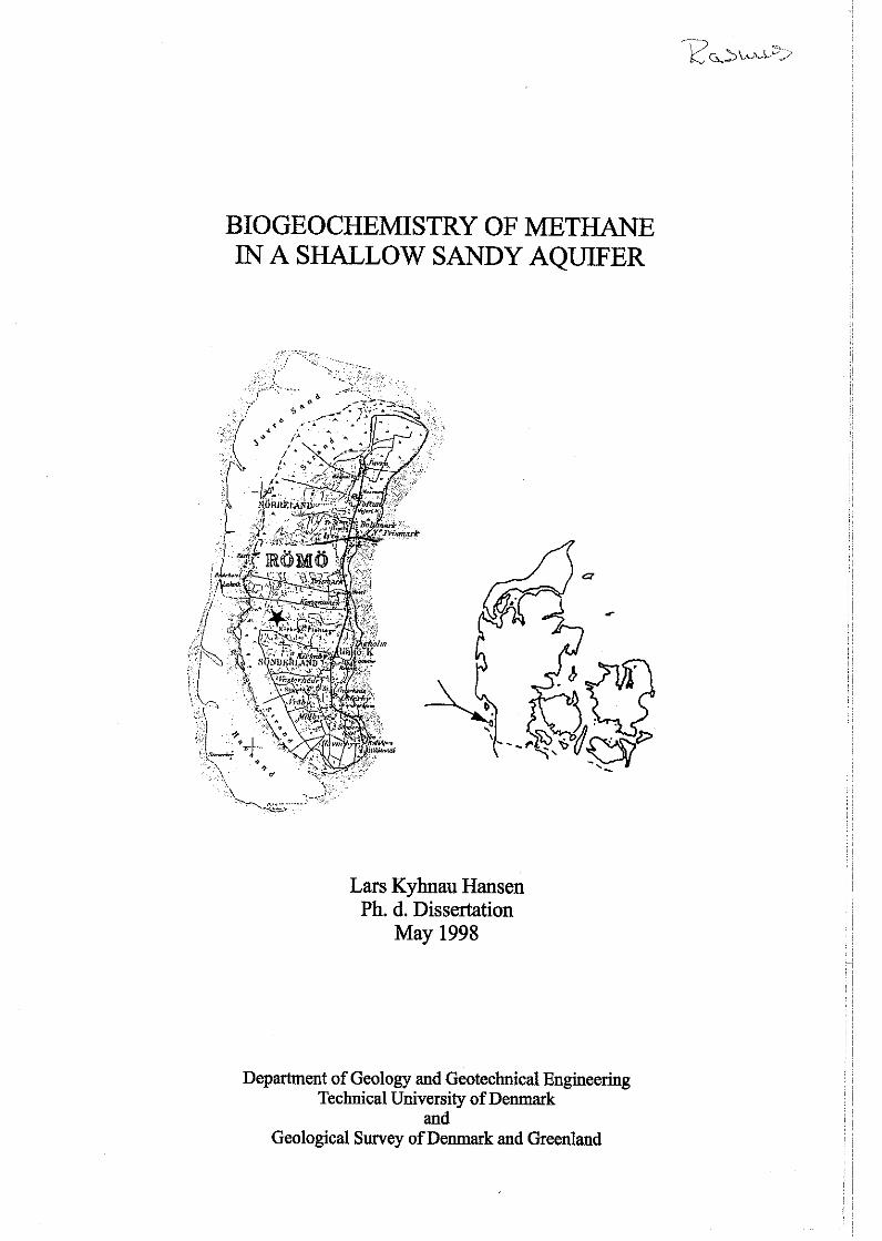
The data for this study are from a young (<2500 years) shallow aeolianlmarine sandy aquifer on
the island of Ram, Denmark. The dissertation describes the first direct measurements of methane
production and methane oxidation rates and the first detailed measurements of formate and acetate
concentrations in an aquifer. Time series canied out for the rate measurements indicate that the
methods are reliable.
Methane production occurs mainly via the CO, reduction pathway, but there is also a significant,
and highly variable, contribution from acetate fermentation. The rates are 1-3 orders of magnitude
lower than those previously measured in marine sediments, but similar to rates measured in some
lake sediments. The rates vary considerably over depth and between sampling locations, which
most likely reflects, that reactive organic matter is unevenly distributed.
Mass balance considerations show, that most of the organic matter used in the redox processes
must come from the soil zone with the infiltrating water, possibly attached to colloids This is
different from deep aquifer systems, where it is usually organic matter, deposited with the
sediment, that is being decomposed.
There is a distinct separation between sulfate reduction and methane production. When sulfate
enters previously methanogenic parts of the aquifer, sulfate reduction replaces methane
production, whereas methane is readily formed in previously sulfate reducing parts of the aquifer,
when sulfate is no longer present. In contrast, sulfate reduction and Fe(II1)-oxide reduction are
not spatially separated. In sulfate free parts of the aquifer, another redox process, possibly Fe(II1)-
oxide reduction, also occurs concurrently with methane production. This redox process is able to
outcompete methane production almost completely in some sulfate free parts of the aquifer, but
not in others. The competitive suppression of methane production occurs concurrently for the CO,
reduction and acetate fermentation pathways.
In contrast to the situation in marine sediments, methane oxidation coupled to sulfate reduction
is not a quantitatively important process. This most likely reflects, that the concentrations of
methane and sulfate are much lower than in marine sediments.
The hydrogen concentration reflects the dominating redox process to some extent, but the energy
yield of CO, reduction is so low, that this process must take place in microniches with higher H,
concentrations or by hydrogen transfer between juxtaposed bacteria. The H, concentration in the
bulk sediment must therefore be controlled by another redox process, e.g. Fe(II1)-oxide reduction,
even when methane production is the dominating redox process. Accordingly, the H, concentra-
tion cannot be used to determine, which redox process dominates.
The concentrations of formate and acetate are completely unrelated to the dominating redox
process. Calculations of the energy available from acetate turnover show, that competitive
suppression of methane production from acetate cannot be due to a limited energy yield of the
process, which is the traditional explanation. It is suggested, that the hydrogen concentration
might control the turnover of acetate by causing acetogenic methanogenic bacteria to switch their
metabolism from CH, production to H, production from acetate, when the H, concentration is low
enough to make this energetically favourable.
IV Dansk resume
De data, som prresenteres i denne afhandling, er fra en ung (<2500 ir) overfladenzer akvifer p i
Rams, Danmark. Akviferen bestir af zeolisk og marint sand. Ailandlingen beskriver de fsrste
direkte milinger af methandannelsesrater og methanoxidationsrater samt de fsrste detaljerede
milinger af format- og acetatkoncentrationer i en akvifer. Tidsserier for ratemilingerne indikerer,
at de anvendte metoder er pilidelige.
Methanproduktionen sker primrert via CO, reduktion, men der er ogsi et vzsentligt og meget
varierende bidrag fra acetatfernentation. De milte rater er 1-3 stsrrelsesordener rnindre end dem,
som tidligere er m3t i marine sediienter, men svarer ti1 de rater, som er milt i nogle sssedimenter.
Raterne varierer meget over dybde og mellem de underssgte prsvetagningssteder, hvilket
sandsynligvis skyldes, at det reaktive organiske materiale er ujzevnt fordelt.
Massebalanceberegninger viser, at hovedparten af det organiske materiale, som bliver forbrugt i
redoxprocesserne, kommer fra jordbunden med det infiltrerende vand, muligvis bundet ti1
kolloider. Dette er forskelligt fra dybe akviferer, hvor det normalt er organisk stof aflejret med
sedimentet, som bliver omsat.
Der er en klar adskillelse mellem sulfatreduktion og methanproduktion. N i r sulfat twnger ind i
tidligere methanogene dele af akviferen, erstattes methanproduktion med sulfatreduktion,
hvorimod methanproduktion straks g i r i gang i tidligere sulfatreducerende dele af akviferen, n t
sulfat ikke izngere er ti1 stede. I modsztning ti1 dette er der ingen adskillelse mellem jern(II1)
reduktion og sulfatreduktion. I de sulfatfrie dele af akviferen foregir en anden redox proces,
muligvis jern(II1) reduktion, ogsi samtidig med methanproduktionen. Denne redoxproces er i
stand ti1 nzsten helt at udkonkurrere methanproduktion i nogle sulfatfrie dele af akviferen, men
ikke i andre. Udkonkurreringen af rnethanproduktion sker bide for CO, reduktions og
acetatfermentations dannelsesvejene.
I modszetning ti1 situationen i marine sedimenter er methanoxidation koblet ti1 sulfatreduktion ikke
nogen kvantitativt vzesentlig proces. Dette skyldes sandsynligvis, at koncentrationerne af sivel
methan som sulfat er meget lavere end i de marine sedimenter.
Hydrogen koncentrationen afspejler i nogen grad den dominerende redoxproces, men
energiudbyttet ved CO, reduktion er s i lavt, at CO, reduktionen m i foregi i mikronicher med
hsjere hydrogen koncentrationer eller ved direkte overfarrsel af hydrogen mellem tretsiddende
bakterier Hydrogen koncentrationen i bulk sedimentet m?i derfor vzre styret af en anden redox
proces, f.eks. jern(II1) reduktion, selv nir methanproduktion er den dominerende redox proces.
Dette betyder, at hydrogen koncentrationen ikke kan bmges ti1 at afgare hvilken redox proces,
som dominerer.
Format og acetat koncentrationeme afspejler slet ikke den dominerende redoxproces. Beregninger
afdet energimzssige udbytte ved acetatomsztning viser, at fravzret af methanproduktion ud fra
acetat i dele af akviferen ikke kan skyldes et lavt energiudbytte ved processen, som det hidtil har
vzret antaget. Det foreslk, at hydrogen koncentrationen styrer omsztningen af acetat, ved at
acetatforbrugende methanogene bakterier skifier fra at producere methan ti1 at producere
hydrogen, nir hydrogen koncentrationen bliver tilstrrekkeligt lav ti], at dette er energimzssigt
fordelagtig.
1. Introduction
The danish water supply has traditionally been based on the utilization of water from shallow
aquifers. However, the water quality in these aquifers is threatened by pollution from numerous
anthropogenic sources: agricultural land use, industry etc. For this reason, an increased interest
has developed in the possibility of utilizing deeper aquifer systems to secure a supply of unpolluted
water. Reduced conditions are often found in such aquifers, and a need has therefore arisen to
know more about, what controls the water chemistry in reduced aquifers .
This project is part of a research program focussing on geochemical processes in reduced aquifers.
While methane in itself does not pose any critical problems to the water supply (it is easily
removed by extended airation of the water), an understanding of the microbiologically mediated
processes, that lead to methane formation in aquifers, might prove important for our ability to
predict the fate of organic pollutants in groundwater.
While reduced conditions are most common in deep aquifers, practical considerations speaks
strongly for choosing a shallow aquifer for a detailed geochemical study as this. Moreover, while
shallow reduced aquifers are geologically and hydrogeologically different from deep aquifers in
many ways (lower sediient age, shorter residence time of the water, no confining aquitards etc.),
the processes are presumably the same. For this reason, the shallow Ram aquifer was chosen for
this study. The &ma aquifer has been subject to previous detailed geochemical investigations,
focussing on sulfate reduction (Jakobsen & Postma, 1994; Jakobsen, 1995) and on Fe(II1)-oxide
reduction (larsen, 1998).
1.1 Decomposition of organic matter and redox processes.
There are two principle sources for organic matter in aquifers. One is organic matter deposited
with the sediient, the other is organic matter leached from the soil zone by infiltrating water. The
latter source seems to be particularly important in aquifers with a shallow water table, because the
short residence time of water in the unsaturated zone allows more organic matter to reach the
saturated zone without being decomposed (Starr, 1988).
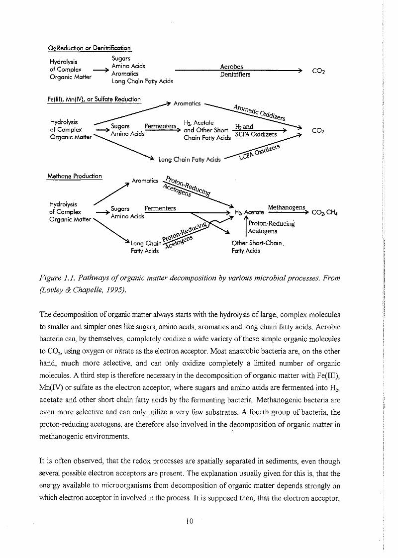
Once present in the aquifer, organic matter can act as an electron donor for a wide range of
bacterially mediated redox processes. The most common of these redox processes are 0,
reduction (aerobic respiration), NO; reduction (denitrification), Mn(1V)-oxide reduction, Fe(II1)-
oxide reduction, SO:- reduction and CO, reduction (methane production). Depending on which
electron acceptor is used in the redox process, the decomposition of organic matter will be carried
out by different strains of bacteria and proceed via different pathways. An overview of these
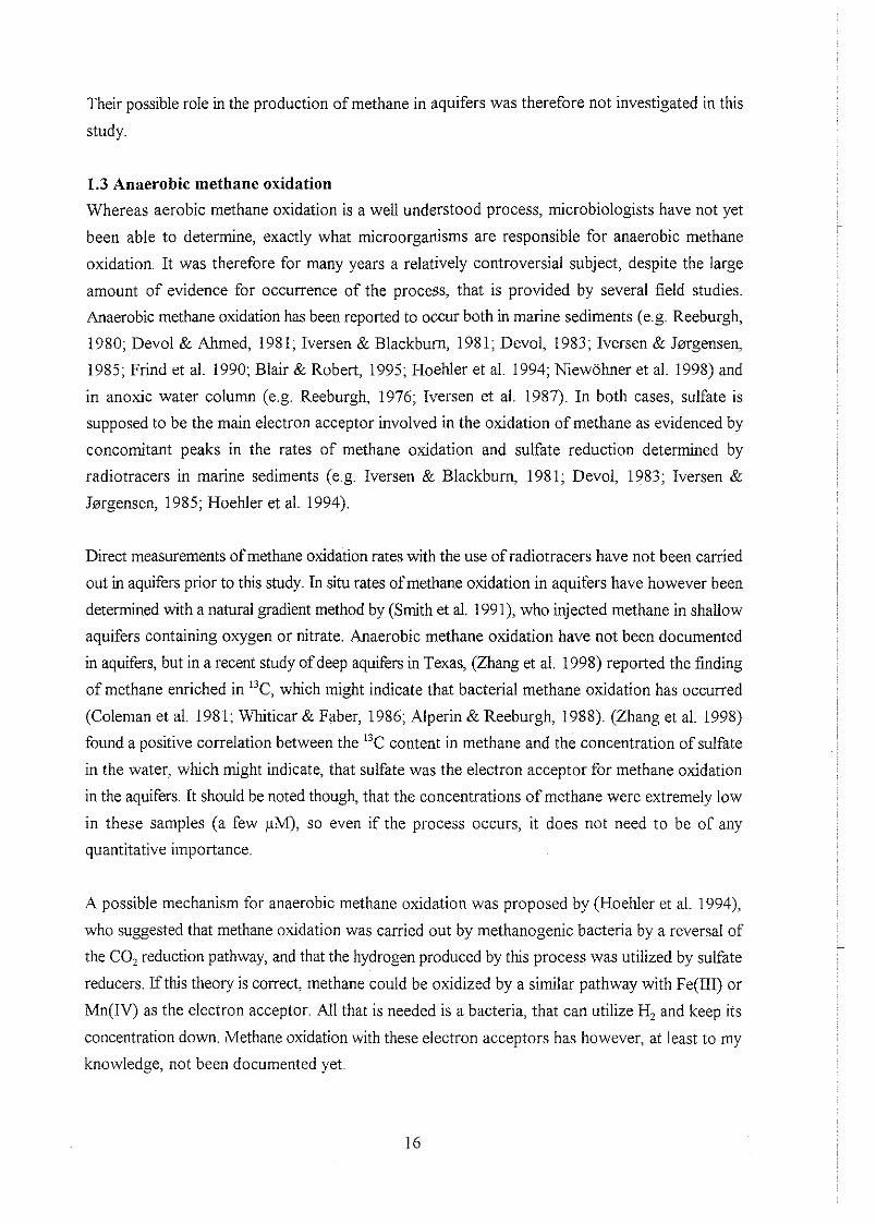
pathways is shown in figure 1.1.
02 Reduction or Denitrificatian
Hydrolysis Sugars
of Complex Amino Acids Aerobes Aromatics Denihifiers co? Organic Matter Long Chain Faity Acids
Fe(lll), Mn(lV), or Sulfate Reduction Aromatics
Hydrolysis Sugars Fermenters HL Acetote
of Complex and Other Short Oxidizers Organic Matter Chain Faity Acids
Long Chain F d y Acids
Methane Production
Hydrolysis Sugars Fermenters Methanogens of Complex
Organic Matter > COB CH4
Other Short-Chain Fatty Acids Fatty Acids
Figure I . I . Pathways of organic matter decomposition by various microbial processes. From
(Lovley & Chapelle, 1995).
The decomposition of organic matter always starts with the hydrolysis of large, complex molecules
to smaller and simpler ones like sugars, amino acids, aromatics and long chain fatty acids. Aerobic
bacteria can, by themselves, completely oxidize a wide variety of these simple organic molecules
to CO, using oxygen or nitrate as the electron acceptor. Most anaerobic bacteria are, on the other
hand, much more selective, and can only oxidize completely a limited number of organic
molecules. A thrd step is therefore necessaly in the decomposition of organic matter with Fe(III),
Mn(1V) or sulfate as the electron acceptor, where sugars and amino acids are fermented into H,,
acetate and other short chain fatty acids by the fermenting bacteria. Methanogenic bacteria are
even more selective and can only utilize a very few substrates. A fourth group of bacteria, the
proton-reducing acetogens, are therefore also involved in the decomposition of organic matter in
methanogenic environments.
It is often observed, that the redox processes are spatially separated in sediments, even though
several possible electron acceptors are present. The explanation usually given for this is, that the
energy available to microorganisms from decomposition of organic matter depends strongly on
which electron acceptor in involved in the process. It is supposed then, that the electron acceptor,
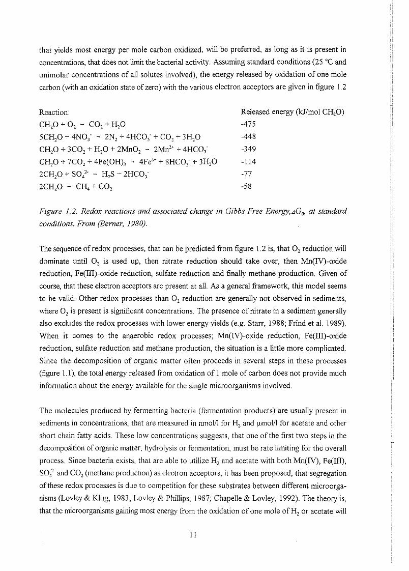
that yields most energy per mole carbon oxidized. will be preferred, as long as it is present in
concentrations, that does not l i t the bacterial activity. Assuming standard conditions (25 "C and
unimolar concentrations of all solutes involved), the energy released by oxidation of one mole
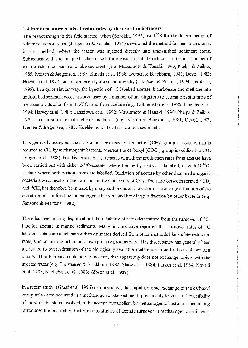
carbon (with an oxidation state of zero) with the various electron acceptors are given in figure 1.2
Reaction: Released energy (kJ1mol CH,O)
CH,O + 0, - CO, + H,O -475
5CH,O + 4NO; - 2N, + 4HCOi + C02 + 3H,O -448
CH,0 + 3C0, + H,0 + 2Mn0, - 2Mn" + 4HCO; -349
CH,0 + 7C0, + 4Fe(OH), - 4Fe2+ + 8HC0; + 3H20 -1 14
2CH,O + SO> - H,S + 2HCOi -77
2CH20 - CH, + CO, -58
Figzrre 1.2. Redox reactions and associated change in Gibbs Free Energy,~G,, at standard
conditions. From (Berner, 1980).
The sequence of redox processes, that can be predicted from figure 1.2 is, that 0, reduction will
dominate until 0, is used up, then nitrate reduction should take over, then Mn(1V)-oxide
reduction, Fe(II1)-oxide reduction, sulfate reduction and finally methane production. Given of
course, that these electron acceptors are present at all. As a general framework, this model seems
to be valid. Other redox processes than 0, reduction are generally not observed in sediments,
where 0, is present is significant concentrations. The presence of nitrate in a sediment generally
also excludes the redox processes with lower energy yields (e.g. Starr, 1988; Frind et al. 1989).
When it comes to the anaerobic redox processes; Mn(1V)-oxide reduction, Fe(II1)-oxide
reduction, sulfate reduction and methane production, the situation is a little more complicated.
Since the decomposition of organic matter often proceeds in several steps in these processes
(figure 1. I), the total energy released from oxidation of 1 mole of carbon does not provide much
information about the energy available for the single microorganisms involved.
The molecules produced by fermenting bacteria (fermentation products) are usually present in
sediments in concentrations, that are measured in nmolll for Hz and pmolll for acetate and other
short chain fatty acids. These low concentrations suggests, that one of the first two steps in the
decomposition of organic matter, hydrolysis or fermentation, must be rate limiting for the overall
process. Since bacteria exists, that are able to utilize Hz and acetate with both Mn(IV), Fe(III),
SO: and CO, (methane production) as electron acceptors, it has been proposed, that segregation
of these redox processes is due to competition for these substrates between different microorga-
nisms (Lovley & Klug, 1983; Lovley & Phillips, 1987; Chapelle & Lovley, 1992). The theory is,
that the microorganisms gaining most energy from the oxidation of one mole of H, or acetate will
grow faster than those gaining less energy, and since the supply of Hz and acetate is limited by one
of the previous steps in the decomposition of organic matter, the concentrations of H, and acetate
will become so low, that less effective microorganisms cannot be active, even though they might
still be present in the sediment. This phenomenon has been termed competitive exclusion.
The concept of competitive exclusion was used by (Lovley & Goodwin, 1988) to show
theoretically, and demonstrate, using data from natural sediments, how competition between
different terminal electron accepting processes (TEAP's) leads to specific levels of Hz for each
redox zone. (Lovley & Goodwin, 1988) predicted typical H2 levels of 0.1-0.5 nM for Fe(II1)-oxide
reduction, 1-3 nM for sulfate reduction and 7-10 nM for methanogenesis. In subsequent studies
of anaerobic aquifers, ranges ofH2 concentrations have been determined to 0.1-0.8 nM for Fe(II1)-
oxide reducing, 1.0-4.0 nM for sulfate reducing and 5-25 nM for methane producing aquifers
(Chapelle & Lovley, 1992; Vroblesky & Chapelle, 1994; Chapelle et al. 1995). (Jakobsen, 1995)
measured Hz concentrations in the Rum aquifer, and found, that the H2 concentration give a poor
picture of the dominant TEAP in this aquifer. In general the H, concentration is lower than
predicted by (Lovley & Goodwin, 1988) and so low, that CO, reduction is not energetically
favourable in parts of the aquifer. However, high concentrations of methane in parts of the aquifer
indicated ongoing methanogenesis. In a later study, similar results were found in a landfill leachate
plume in Gnndsted, Denmark by (Jakobsen et al. 1998).
(Jakobsen, 1995; Jakobsen et al. 1998) explained the lack of correlation between Hz concentration
and TEAP by concurrent occurrence of the redox processes and also suggested, that CO,
reduction must take place within microniches with higher H2 concentrations or by interspecies
hydrogen transfer between juxtaposed bacteria, as previously proposed by (Conrad et al. 1985;
Thiele & Zeikus, 1988).
In a review of sulfate reduction and Fe(II1)-oxide reduction in sediments, (Postma & Jakobsen,
1996) found that these two processes often seems to occur concurrently. An explanation for this
was sought in the thermodynamics of the two processes under in situ conditions, and (Postma &
Jakobsen, 1996) concluded, that concurrent reduction ofFe(IU)-oxides and sulfate is thermodyna-
mically possible under a vide range of natural conditions, depending among other things on the
reactivity ofFe(1II)-oxides and, in Fe2' rich porewater, on the pH of the porewater Under some
conditions, sulfate reduction is more energetically favourable than reduction of less reactive
Fe(III)-oxides. Accordingly, (Postma & Jakobsen, 1996) proposed a slightly different explanation
for the segregation of the anaerobic redox processes, where the fermenting step is thought to be
rate limiting and the electron accepting processes are considered to be close to equilibrium. Using
this approach, the sequence of redox processes shown in figure 1 2 can again be predicted, but
only when the in situ AG~'s are significantly different. When this is not the case, the partial
equilibrium model predicts, that the redox processes might occur concurrently
The TEAP's do not occur at true equilibrium, since the bacteria must gain sufficient energy from
the process to enable cell growth. (Hoehler, 1998) for instance reported, that CO, reduction in
Cape Lockout Bight occurred at AG, values near -10 to -15 kJ1mole Hz, whereas sulfate reduction
occurred at a slightly higher energy yield (more negative AG,). (Hoehler, 1998) also found, that
temperature, pH and the concentration of sulfate had a large influence on the Hz concentration,
presumably due to the resulting changes in AG,. This supports the hypothesis, that the H,
concentration is thermodynamically controlled, and that the bacteria keeps it as close to
equilibrium as biologically possible. However, there is no reason to expect specific Hz
concentration levels for specific TEAP's. Rather one should expect to find a AG, value for the
dominating TEAP, that is close to the biologically determined threshold level. The Hz concentra-
tion will then be controlled, not only by the dominating TEAP, but also by the temperature and
the activity of the various solutes involved in the reactions, as proposed by (Postma & Jakobsen,
1996).
1.2 Methane in aquifers and methanogenic pathways
Most previous studies of methane in aquifers have focussed on whether the methane is
thermogenic or bacterial in origin. A classic tool for this purpose is to look at the relation between
CH, and longer chain hydrocarbons (C,-C,). Bacterially produced methane never contains
significant amounts of (C,-C,) hydrocarbons, and a high content of these (>0.05 %) is therefore
a very good indicator of a non bacterial origin of the methane (Schoell, 1980).
Another tool often used to classify methane is the relation between light and h e a ~ y isotopes of
carbon and hydrogen (13C/12C and Dm). In bacterially mediated processes, light isotopes are
consumed preferentially to heavy isotopes, and accordingly bacterially formed methane is depleted
in 13C and D relative to the parent material: CO, and H,O. Furthermore, methanogens that produce
methane !?om H,/CO, usually have larger fractionation factors for 13C/12C than those producing
methane from acetate (Whiticar et a1 1986). It is therefore generally found, that methane, that is
produced by CO, reduction contains less (is more depleted in) "C than methane, that is produced
by acetate fermentation. On the other hand, methane, this is produced from acetate, is usually far
more depleted in D than methane, that is produced from H2/C0,. This is due mainly to the fact,
that all four hydrogen atoms are derived from water in methane, that is produced by CO,
reduction, whereas three of the four hydrogen atoms are derived from organic matter (acetate) in
methane, that is produced by acetate fermentation (Whiticar et al. 1986). A classification diagram
for methane, based on data from a number of lake and marine sediments is shown in figure 1.3.
Figure I . 3. Natural gas genetic classification diagram using 6°C and 6D in methane. From
(Whiticar et al. 1986).
Thennogenic methane usually have 613C values in the -20 to -40 "/,, range, whereas 613C values
in the -40 to -110 "I,, range indicate a bacterial origin of the methane (Whiticar et al. 1986).
Isotopically heavy methane (6I3C > -40 '1,) might however also be the result of methane oxidation
(Coleman et al. 1981; Whiticar & Faber, 1986; Alperin & Reeburgh, 1988) or of reservoir effects,
when a significant part of the TIC (Total Inorganic Carbon) pool is turned over to methane
(Whiticar et al. 1986). Methane produced by acetate fermentation and by CO, reduction differ
mainly on the 6 D value, with 6D values < -250 %, being typical for acetate fermentation
(Whiticar et al. 1986).
A more recent classification diagram, based on deuterium and used for methane in Canadian
aquifers by (Aravena et al. 1995), is shown in figure 1.4. This diagram will be used in section 4.5
to estimate the relative contribution of CO, reduction and acetate fermentation to methane
production in the R0m0 aquifer.
Most studies have shown acetate fermentation to be the primary pathway of methane production
in lake sediments (e.g. Kuivila et al. 1988), whereas CO, reduction dominates in marine sediments
(e.g. Crill &Martens, 1986). All previous studies of bacterial methane from aquifers, that I know
of, have showed an isotopic composition of methane, that indicates CO, reduction to be the main
pathway of methane production in aquifers (Coleman et al. 1988; Grossman et al. 1989; Barker
& Fritz, 1981; Aravena et al. 1995).
OVERBURDEN WELLS a BEDROCK WELLS
Figure 1.4. Classzfication diagram for bacterial methane. l7ze line 0:IOO indicate 100 % COz
reduction, the line 20:80 indicate 20 % ncetate fermentation and 80 % CO, reduction etc. From
Pravena et al. 1995).
Despite the large number of studies concerning bacterial methane formation in sediments, little is
still known about what factors influence the relative importance of the different pathways. Factors,
that have been proposed to be important, are the temperature and the age of organic matter
(Schoell, 1988). High temperatures and young organic matter are associated with acetate
fermentation, whereas low temperatures and old organic matter are associated with CO, reduction.
(Hoehler, 1998) suggested, that some of the d'ierence in methanogenic pathways between marine
and lake sediments might be related to the different pH values and ionic strengths found in these
environments.
Besides acetate and H,, methanogenic bacteria are also able to utilize a few other substrates like
formate, methanol, methane thiol, dimethylsulfide and methylated amines (Oremland et al. 1982;
Oremland & Polcin, 1982; King, 1984; Oremland, 1988). The latter four substrates are often called
"noncompetitive", because they cannot be utilized by sulfate reducing bacteria Noncompetitive
substrates might be responsible for the occurrence of some methane production in sulfate reducing
sediments, but have, to my knowledge, only been reported to be significant for the total
production of methane in salt marsh sediments (Oremland et al. 1982; Oremland & Polcin, 1982).
Their possible role in the production of methane in aquifers was therefore not investigated in this
study.
1.3 Anaerobic methane oxidation
Whereas aerobic methane oxidation is a well understood process, microbiologists have not yet
been able to determine, exactly what microorganisms are responsible for anaerobic methane
oxidation. It was therefore for many years a relatively controversial subject, despite the large
amount of evidence for occurrence of the process, that is provided by several field studies.
Anaerobic methane oxidation has been reported to occur both in marine sediments (e.g. Reeburgh,
1980; Devol & Ahmed, 1981; Iversen & Blackbum, 1981; Devol, 1983; Iversen & Jerrgensen,
1985; Frind et al. 1990; Blair & Robert, 1995; Hoehler et al. 1994; Niewohner et al. 1998) and
in anoxic water column (e.g. Reeburgh, 1976; Iversen et al. 1987). In both cases, sulfate is
supposed to be the main electron acceptor involved in the oxidation of methane as evidenced by
concomitant peaks in the rates of methane oxidation and sulfate reduction determined by
radiotracers in marine sediments (e.g. Iversen & Blackburn, 1981; Devol, 1983; Iversen &
Jerrgensen, 1985; Hoehler et al. 1994).
Direct measurements of methane oxidation rates with the use of radiotracers have not been carried
out in aquifers prior to this study. In situ rates of methane oxidation in aquifers have however been
determined with a natural gradient method by (Smith et al. 1991), who injected methane in shallow
aquifers containing oxygen or nitrate. Anaerobic methane oxidation have not been documented
in aquifers, but in a recent study of deep aquifers in Texas, (Zhang et al. 1998) reported the finding
of methane enriched in 13C, which might indicate that bacterial methane oxidation has occurred
(Coleman et al. 1981; Whiticar & Faber, 1986; Alperin & Reeburgh, 1988). (Zhang et al. 1998)
found a positive correlation between the 13C content in methane and the concentration of sulfate
in the water, which might indicate, that sulfate was the electron acceptor for methane oxidation
in the aquifers. It should be noted though, that the concentrations of methane were extremely low
in these samples (a few pM), so even if the process occurs, it does not need to be of any
quantitative importance.
A possible mechanism for anaerobic methane oxidation was proposed by (Hoehler et al. 1994),
who suggested that methane oxidation was carried out by methanogenic bacteria by a reversal of
the CO, reduction pathway, and that the hydrogen produced by this process was utilized by sulfate
reducers. If this theory is correct, methane could be oxidized by a similar pathway with Fe(I1I) or
Mn(IV) as the electron acceptor. All that is needed is a bacteria, that can utilize H, and keep its
concentration down. Methane oxidation with these electron acceptors has however, at least to my
knowledge, not been documented yet.
1.4 In situ measurements of redox rates by the use of radiotracers
The breakthrough in this field started, when (Sorokin, 1962) used 3 5 ~ for the determination of
sulfate reduction rates. (Jsrgensen & Fenchel, 1974) developed the method further to an almost
in situ method, where the tracer was injected directly into undisturbed sediment cores.
Subsequently, this technique has been used for measuring sulfate reduction rates in a number of
marine, estuarine, marsh and lake sediments (e.g. Matsumoto & Hanaki, 1990; Phelps & Zeikus,
1985; Iversen & Jsrgensen, 1985; Kuivila et al. 1988; Iversen & Blackburn, 1981; Devol, 1983;
Hoehler et al. 1994), and more recently also in aquifers by (Jakobsen & Postma, 1994; Jakobsen,
1995). In a quite similar way, the injection of '"C labelled acetate, bicarbonate and methane into
undisturbed sediment cores has been used by a number of investigators to estimate in situ rates of
methane production from HJCO, and from acetate (e.g. Crill & Martens, 1986; Hoehler et al.
1994; Harvey et al. 1989; Lansdown et al. 1992; Matsumoto & Hanaki, 1990; Phelps & Zeikus,
1985) and in situ rates of methane oxidation (e.g. Iversen & Blackburn, 1981; Devol, 1983;
Iversen & Jsrgensen, 1985; Hoehler et al. 1994) in various sediments.
It is generally accepted, that it is almost exclusively the methyl (CH,) group of acetate, that is
reduced to CH, by methanogenic bacteria, whereas the carboxyl (COO3 group is oxidized to CO,
(Vogels et al. 1988). For this reason, measurements of methane production rates from acetate have
been carried out with either 2-14C-acetate, where the methyl carbon is labelled, or with U-'T-
acetate, where both carbon atoms are labelled. Oxidation of acetate by other than methanogenic
bacteria always results in the formation of two molecules of CO,. The ratio between formed 14C0,
and I4CH4 has therefore been used by many authors as an indicator of how large a fraction of the
acetate pool is utilized by methanogenic bacteria and how large a fraction by other bacteria (e.g.
Sansone & Martens, 1982).
There has been a long dispute about the reliability of rates determined from the turnover of 14C-
labelled acetate in marine sediments. Many authors have reported that turnover rates of 14C
labelled acetate are much higher than estimates derived from other methods like sulfate reduction
rates, ammonium production or known primary productivity. This discrepancy has generally been
attributed to overestimation of the biologically available acetate pool due to the existence of a
dissolved but biounavailable pool of acetate, that apparently does not exchange rapidly with the
injected tracer (e.g. Christensen & Blackbum, 1982; Shaw et al. 1984; Parkes et al. 1984; Novelli
et al. 1988; Michelson et al. 1989; Gibson et a1 1989).
In a recent study, (Graaf et al. 1996) demonstrated, that rapid isotopic exchange ofthe carboxyl
group of acetate occurred in a methanogenic lake sediment, presumably because of reversibility
of most of the steps involved in the acetate metabolism by methanogenic bacteria. This finding
introduces the possibility, that previous studies of acetate turnover in methanogenic sediments,
that have used U-"C-acetate as the tracer, might have seriously overestimated the rate of acetate
oxidation as well as the fraction of acetate, that was consumed by other than methanogenic
bacteria. It should be noted though, that "too fast" turnover of U-I4C-acetate has also been
reported in sulfate reducing sediments. and (Graaf et al. 1996) found no evidence for isotope
exchange in acetate, when sulfate was the electron acceptor In this study, 2-"C-acetate was used,
which eliminates the problem of isotope exchange of the carboxyl carbon, since only the methyl
carbon is labelled. No attempts were made to quantify the size of a possible biologically
unavailable pool of dissolved acetate, but as will be shown in the following sections. the acetate
turnover rates measured in the b n w aquifer are generally not suspiciously high compared to other
estimates of organic matter decomposition in the aquifer, so this is probably not a serious problem
Perhaps because a sandy aquifer is physically and chemically different from marine sediments in
many ways: lower ionic strange of the water, lower adsorption capacity of the sediment due to a
much smaller content of clay and organic matter etc.
Most previous measurements of methane oxidation rates with '"C labelled methane also seems to
have been hampered by a potentially very serious problem In a recent study (Harder, 1997) found
that the bacterially produced "CH,, that have been used in many previous studies of methane
oxidation rates, contains I4CO in amounts of up to %-I % of the '"CH,. According to (Harder,
1997), CO is readily oxidized to CO, by bacteria (e.g. sulfate reducing), that are able to carry out
carbonmonooxide-dehydrogenase, and such bacteria are widespread in marine habitats. Since the
CO pool in sediments is several orders of magnitude smaller than the CH, pool (nmoV1 rather than
mmofl), rapid turnover of unintentionally injected "CO might be responsible for a large fraction
of the I4CO2 fonned in many previous studies of methane oxidation. According to (Harder, 1997)
only (Iversen & Jsrgensen, 1985) achieved a high enough turnover of the injected CH, tracer in
their experiments to exclude the possibility, that formed 'TO, was derived solely from
contaminant '"0.
It is uncertain though, to how large an extent the results from previous studies of methane
oxidation rates have to be discarded for this reason. The measured rates have usually been
supported by concentration profiles and they have been strongly depth dependent despite the likely
(although not always documented) presence of sulfate reducing bacteria at all depths Finally time
series have shown linear rates, which indicate, that only one compound in being consumed and that
its concentration is not seriously depleted during the incubation. All in all it seems like further
studies of CO cycling and methane oxidation in sediments are necessary, before all previous
studies of methane oxidation rates using I4CH4 are discarded. In this study ITCH, was purified from 14 CO by treatment with Hopcalite, as recommended by (Harder. 1997), to avoid the problem
2. Methods
Many of the methods used are more or less standard methods and will only be described briefly.
Others have been developed or implemented as a part of this investigation and will be described
and discussed in more detail.
2.1 Collection of water samples
Most of the water samples were taken from driven wells. A filter tip with a 6 cm long stainless
steel 50 pm screen was driven down with 1" steel pipe using a pneumatic gasoline driven Pioneer
hammer. The filter tips had check valves so that samples could be taken by gas displacement using
nitrogen. In May 1996, the samples from 1-5 m.b.s. were taken from a driven well with a stainless
steel 50 pm screen, only 1 cm long. The screen was connected directly to a 118" stainless steel
tubing running inside the driving pipe to the surface. This enabled water to be pumped in small
amounts (< 100 ml) from very distinct depths of the aquifer, using a peristaltic pump. In this way
an exceptionally low distance between sampling points (2-5 cm) was obtained.
Water for measurements of H, concentrations cannot be taken from driven wells, because
hammering of the steel pipes leads to production of Hz (Jakobsen, 1995; Bjerg et al. 1997). For
this reason, 16 rnrn outer diameter PVC tubes, equipped with a 20 pm Nylon screen, were installed
in shallow wells, drilled with hand-tools, using plastic casing and a stainless steel bailer. It was
found by (Jakobsen, 1995; Bjerg et al. 1997), that this method minimizes the risk of introducing
metal to the magazine, that might produce hydrogen through contact with water. It was found by
(E3jerg et al. 1997), that a 1-2 month equilibration time is needed after installing such wells, before
H, concentrations are back to natural levels. For this reason the PVC wells were all installed in
December 1996, but left until March 1997, before water was pumped for Hz analysis.
In July 1997 all water samples were taken from the installed PVC wells, using 8 mm outer
diameter teflon tubing and a peristaltic pump. Apart from convenience, this method had the
advantage of enabling the determination of H, concentrations at the exact same spots in the
aquifer, where all other components were determined. Except for some problems with insufficient
flushing of the PVC wells prior to sampling for formate and acetate, there were no general
differences comparing 1996 to 1997 data, that could be attributed to the different ways of
sampling.
All water samples, except those only used for analysis of CH,, were filtrated in the field, most of
them using a 0.2 pm syringe tip filter. Samples for analysis of anions (Cl-, SO:- and NO,?, NH,' and organic acids (formate, acetate and propionate) were taken in 5 ml. polypropylene
scintillations vials, frozen at the field site and kept frozen (-18 "C) until analysed. Samples for
measurement of cations (Ca, Mg, Na, K and Mn) were taken in 50 ml plastic vials, acidified by
adding 0.5 % concentrated nitric acid and stored at 5 "C until analysed. Samples for analysis of
DOC were taken in 25 ml or 50 ml. glass vials, equipped with teflon coated screw caps. The glass
vials were rinsed by soaking in 30 % nitric acid for 24 hours and subsequent heating to 550 "C.
TheDOC samples were also acidified, adding 0.2 % concentrated nitric acid, and stored at 5 "C
until analysed.
Two different methods were used for collecting water samples for measurement of CH,
concentrations.
The standard method, that also allowed determination of TIC in the same sample, was to collect
water in a syringe (without contact with the atmosphere) and inject it into an evacuated Venoject
blood sample vial, that was frozen (upside down) at the field site and kept frozen until shortly (1
hour at most) before analysed. Freezing was necessary mainly to avoid adsorption of CO, to the
butyl rubber stoppers in the blood sample vials, when TIC was to be determined in these samples.
As much as 50 % of the CO, and minor amounts of CH, was found to disappear from not frozen
samples in just 24 hours. Filtration was necessary only when TIC was to be determined, the
purpose being to avoid possible contamination fiom small pieces of carbonate, that would be
dissolved by the acid added before analysis to turn HCO; and CO?. into CO,. It was found that
this filtration resulted in only minor losscs of CH,, if it was carried out fast. Normal, not gas tight,
syringes were used for collection of CH,+TIC samples, since tests showed the effect of this to be
negligible, as long as the transference of samples was done fast.
The second method used for collecting CH, samples was implied only for samples, where the
isotopic composition of methane was to be determined along with the methane concentration. A
100 ml serum bottle containing 1 rnl of concentrated sulfuric acid for conservation purposes was
filled with water coming directly from the 8 mm. teflon tube used to transfer water from the
bottom of the wells to the surface. The teflon tube was placed near the bottom of the serum bottle
to minimize the waters exposure to atmospheric air. The first water, that entered the serum vials,
was nonetheless exposed to atmospheric air for some time. It was therefore replaced by overfilling
the serum vial for about 5 seconds. The serum bottle was then closed immediately with a teflon
coated butyl rubber stopper.
A comparison between the results obtained by these two methods showed, that the CH,
concentrations found were usually very similar, when < 0.2 rnM of CH, was measured. When >
0.2 mM of CH, was measured, higher concentrations were always found in the serum vials than
in the blood sample vials (data not shown). Measurements of CH, concentrations in whole
undisturbed sediment cores gave results, that were very similar to those found in the serum vials.
This indicates, that the concentrations determined in blood sample vials are slightly lower than the
actual concentrations. when the methane concentration is above 0.2 mM.
The reason for this is probably, that water with > 0.2 mM of methane is supersaturated with
dissolved gases at surface pressure. Formation of small air bubbles was often observed when water
Eom methanogenic parts ofthe aquifer was collected in syringes. It seemed impossible to sample
these bubbles in a representative way, and it was therefore carefully avoided to transfer them to
the blood sample vials. Since TIC was measured in the same samples, these measurements could
also have been affected slightly by the observed bubble formation in the syringes. TIC was
however present mainly as HCO; in most of the samples, where CH, concentrations were > 0.2
mM, which will have minimized loss of TIC to these bubbles. Moreover, CO, is much more
soluble in water than the other gases present (CH, and N,), and for this reason alone, loss of CO,
to such bubbles will be much smaller relatively.
2.2 Water analysis
Field measurements included alkalinity by the Gran titration method and Fez' by the Ferrozine
method, originally described by (Stookey, 1970). 0, and pH were measured, using electrodes, in
a closed flow cell, that prevented contact with the atmosphere. 0, was never found in
concentrations, that were sipficantly above background levels, and therefore no data are shown
for 0,.
In the laboratory, anions were determined by IC (Ion Chromatography) with W (Ultraviolet) and
EC (Electrical Conductivity) detection. NH,' was determined by FIA (Flow Injection Analysis)
and organic acids by IEC (Ion Exclusion Chromatography), using a Dionex AS-10 column and
suppressed EC detection. The AS-10 column is specially developed for analysis of low
concentrations of organic acids and a Dionex EC suppressor was used to further enhance the
sensitivity of the analysis. The analysis of fermentation products is described more detailed in
section 2.5. Cations CNa, K, Ca, Mg and Mn) were determined by AAS (Atomic Absorption Spec-
troscopy) and DOC (Dissolved Organic Carbon) on a DOHRMAN DC 180 TOC Analyser by
UViPersulfate oxidation and IR (InfraRed) detection.
In general, there was a reasonable electro neutrality in the individual samples, with a deviation
between the sum of anions and cations of less than 5 %. Some of the samples did however show
deviations as large as 10-15 %, but this could generally be attributed to individual errors in the
measurement of alkalinity. The analysis of Na' was not completely without problems either An
apparent change in the concentration of Na' over 4 months at one of the sampling locations
showed a large degree of co-variation with the change in deviation from electro neutrality and was
therefore attributed to systematic errors in the determination ofNa-.
CH, and TIC were measured by injection of 0.2-1.0 ml of headspace gas to a SRI 8680 GC (Gas
Chromatograph), equipped with a FID (Flame Ionization Detector) for analysis of CH, and other
hydrocarbons and a TCD (Thermal Conductivity Detector) for analysis of all gasses. The original
concentration in the sample was calculated from the concentration measured in the headspace, the
volume of sample and headspace and the solubility constant of the gas. The SRI 8680 GC is
portable, and often these analysis were performed during the field trip, sometimes even in the field,
to get a quick overview of the redox conditions in the aquifer.
2.3 Sediment analysis
SOC (Sedimentary Organic Carbon) was measured by a method, where the SOC is split into two
fractions. One fraction is ADOC (Acid Desorbable Organic Carbon), the other, NADOC (Non
Acid Desorbable Organic Carbon) is the organic carbon in the residue. ADOC was determined on
a DOHRMAN DC 180 TOC analyser by UVPersulfate oxidation and IR detection. NADOC and
total carbon was measured by IR detection on a LECO CS-225 Carbon-Sulfur detector. SIC
(Sedimentary Inorganic Carbon) was calculated as the dserence between total carbon and the two
organic fractions.
2.4 Measurement of fermentation product concentrations
The measurement of fermentation product concentrations gives rise to special problems, because
these components are present in very small concentrations and are quite unstable. Hydrogen has
to be measured in the field, as the very small (nM) concentrations change fast during transport or
storage. Hydrogen was measured by the bubble stripping method, that was developed by (Chapelle
& McMahon, 1991) with the modifications made by (Jakobsen, 1995). The samples were analysed
on a TRACEANALYTICAL RGD2 reduced gas detector.
Measurements of organic acid concentrations are not quite so sensitive, since these components
are present in concentrations, that are about 3 orders of magnitudes larger than the concentration
of hydrogen. Still it is necessary to take great care to avoid pollution of the samples and changes
in the concentrations due to microbial activity. Freezing was found to be the best method to avoid
the latter problem. It was found, that the concentration of formate and acetate did not change
significantly over a four month period in frozen (-18 "C) samples, even though these had been
thawed for a few hours, when the first measurement was made. Samples from the b m s aquifer
always showed increasing concentrations of formate and acetate, if they were not kept frozen,
presumably because DOC in the samples was decomposed to acetate and formate. In contrast
standards prepared in MilliQ always showed decreasing concentrations of formate and acetate,
presumably due to oxidation of these. To minimize this problem, 0.2 % chloroform was added to
both standards and samples and they were always analysed within 12 hours after thawing or
preparation.
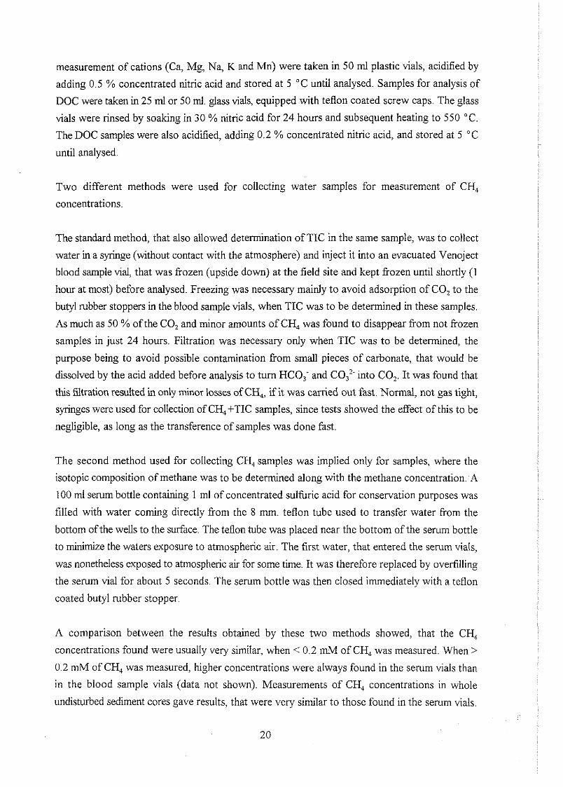
Pollution peaks is another very disturbing problem in the analysis of organic acids, particularly
when the concentrations are low. To minimize these problems, all glass equipment used for the
analysis was rinsed by soaking in 1 M HCI for 12 hours. Even when this was done, there was
sometimes pollution peaks in blinds, that had the same retention time as acetate or more often
formate. Polypropylene was found to be a much better material than glass with regard to avoiding
pollution of organic acid samples, and for that reason 5 ml polypropylene scintillation vials were
used for collecting the samples. No adsorption of organic acids to these vials was observed in
experiments, perhaps because the samples were kept frozen. In contrast, the use of polypropylene
autosampling vials was not possible due to rapid (< 12 hours) adsorption of organic acids to these
vials. Adsorption to filters was not a problem, but many kinds of syringe tip filters could not be
used, because they polluted the samples with acetate.
System peak
I
6.OE+04
Unknown Lactate Forrnate Acetate 4.OE+04 I I I I
2.OE+04
O.OE+OO
I
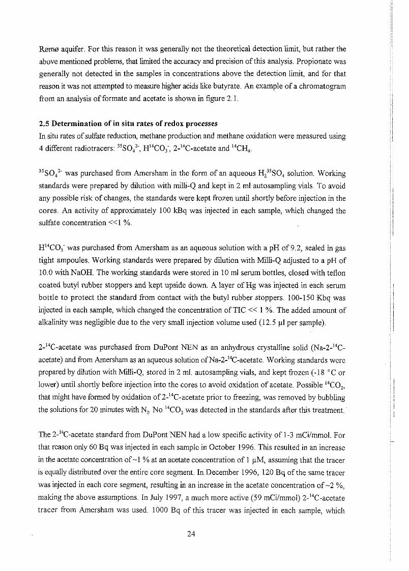
6.00 8.00 10.00 12.00 [min]
Figure 2.1. Chromatogram showirig peaks related to formate and acetate in a samplej?om the
Romn aquqer.
The detection limit of the method depends strongly on avoiding contaminants and on the natural
composition of the sample. If other substances in the sample give large peaks near the retention
time of formate and acetate, the formate and acetate peaks might not be detected, if they are very
small. In samples without interfering peaks, as little as 0.2 pM formate or acetate could be
detected, which is almost one order of magnitude lover than the concentrations measured in the
b m aquifer. For this reason it was generally not the theoretical detection limit, but rather the
above mentioned problems, that limited the accuracy and precision of this analysis. Propionate was
generally not detected in the samples in concentrations above the detection limit, and for that
reason it was not attempted to measure higher acids Like butyrate. An example of a chromatogram
from an analysis of formate and acetate is shown in figure 2.1.
2.5 Determination of in situ rates of redox processes
In situ rates of sulfate reduction, methane production and methane oxidation were measured using
4 different radiotracers: 35S0,2-, H14COi, 2-"C-acetate and 14CH,.
35S042- was purchased from Amersham in the form of an aqueous H;'SO, solution. Working
standards were prepared by dilution with milli-Q and kept in 2 ml autosampling vials. To avoid
any possible risk of changes, the standards were kept frozen until shortly before injection in the
cores. An activity of approximately 100 kE3q was injected in each sample, which changed the
sulfate concentration <<1 %.
H'TO; was purchased from Amersham as an aqueous solution with a pH of 9.2, sealed in gas
tight ampoules. Working standards were prepared by dilution with Milli-Q adjusted to a pH of
10.0 with NaOH. The working standards were stored in 10 ml serum bottles, closed with teflon
coated butyl rubber stoppers and kept upside down. A layer of Hg was injected in each serum
bottle to protect the standard from contact with the butyl rubber stoppers. 100-150 Kbq was
injected in each sample, which changed the concentration of TIC << 1 %. The added amount of
alkalinity was negligible due to the very small injection volume used (12.5 p1 per sample).
2-'"-acetate was purchased from DuPont NEN as an anhydrous crystalline solid (Na-2-'"C-
acetate) and from Amersham as an aqueous solution of Na-2-I4C-acetate. Working standards were
prepared by dilution with Milli-Q, stored in 2 ml. autosampling vials, and kept frozen (-18 "C or
lower) until shortly before injection into the cores to avoid oxidation of acetate. Possible '"CO,,
that might have formed by oxidation of 2-'"C-acetate prior to freezing, was removed by bubbling
the solutions for 20 minutes with N,. No 'TO, was detected in the standards after this treatment.
The 2-%-acetate standard from DuPont NEN had a low specific activity of 1-3 mCi/rnmol. For
that reason only 60 Bq was injected in each sample in October 1996. This resulted in an increase
in the acetate concentration of -1 % at an acetate concentration of 1 pM, assuming that the tracer
is equally distributed over the entire core segment. In December 1996, 120 Bq of the same tracer
was injected in each core segment, resulting in an increase in the acetate concentration of -2 %,
making the above assumptions. In July 1997, a much more active (59 mCi/mmol) 2-14C-acetate
tracer from Amersham was used. 1000 Bq of this tracer was injected in each sample, which

resulted in an increase in the acetate concentration of < 1 %, making the above assumptions.
I4CH4 was purchased from Amersham as a gas in evacuated and sealed glass vials. Since only 45
1.11 of 14CH, was present in each vial, 4-5 ml of Nz was used to dilute the standard for convenient
handling. The diluted "CH, standard was transferred to a 10 ml evacuated serum vial, using a gas
tight syringe. This serum vial contained Hopcalite, that oxidized contaminant '"0 to "CO,, as
recommended by (Harder, 1997). The vial was shaken numerous times to facilitate this oxidation.
After treatment with Hopcalite, the "CH, standard was transferred to another serum vial, filled
with Hg. In this vial, a small amount of concentrated NaOH was injected, and the vial was shaken
to facilitate uptake of "CO, in the base. The base was then removed from the serum vial and the
treatment repeated 5 times to ensure complete removal of 'TO, with minimal loss of 'TH, to the
base. Pressure equilibrations during cleaning and injection of 14CH4 was made by injec-
tinglremoving Hg from the serum vial. After this treatment, no 14C02 or I4C0 was detected in the
I4CH4 standard. Approximately 2000 Bq "CH, was injected in each sample, which resulted in
increases in the CH, concentration of << 1 %, except at very low CH, concentrations.
It was attempted to minimize the injection of oxygen in the cores by bubbling the various aqueous
tracers with N2 and by using Nz rather than atmospheric air for dilution of the I4CH, tracer. No
attempts were made to assure complete absence of oxygen in the tracers However, calculations
showed, that even at saturation with atmospheric air, the amount of oxygen injected in each
sample by the injection of tracer would be used up very fast by inorganic reactions involving e.g.
dissolved Fez', that was always present in the samples. It is therefore highly unlikely, that the
minor amounts of oxygen injected with the tracers could have affected the microbiology in the
samples, except very close to the injection lines.
2.5.1 Collection and incubation of samples
Sediment samples for measurements of radiotracer rates were taken in 50152 rnm innerlouter
diameter stainless steel tubing, using the system developed by (Starr & Ingleton, 1992). The
advantage of this system is, that it is hand operated and that only the sampling tube itself enters
the sediment. This leads to minimal risk of disturbing or polluting the sediment collected To ease
sampling, a shallow well with plastic casing was drilled with hand tools for each core to slightly
above the depth, where the core was to be taken At one location (lo), each of the long (5 m)
cores were taken in one piece, using a 6 m tube. At the other two locations (3 and 8), tube lengths
of 3-4 m were used, and each of the long (5 m) cores was taken in two separate tubes. When an
upper core had been taken at these locations, a new shallow well was drilled at the exact same spot
for collection of a deeper core. The upper samples from these second, deeper cores were taken
in sediment, that had been disturbed by the previous coring and by the hand drilling. Still the rates
measured in these samples did not deviate significantly from those measured in other samples and
they are therefore thought to be reliable and are included in the data presented in section 4.4
After collection of a core, it was (generally within one hour) cut into pieces of 25-50 cm, each of
them closed with plastic stoppers at the ends and sealed with water and diffusion tight tape. After
cutting and sealing, the cores were placed in a hand drilled well with plastic casing for 1-3 hours
to bring them back to in situ temperature and to allow eventual settling of the sediment in the core
to occur, before injection of tracer was made.
In 1996, injections were made in 40 or 50 cm core pieces (when possible) with 8 cm intervals, the
lowest injection being just 4 cm above the bottom of each core piece. Not all of these samples
were analysed, which is why larger distances sometimes exists between the sampling points in the
rates measured in 1996. Even though the sediment in the ends of the cores could have been
~nfluenced by its short contact with atmospheric air, the rates measured at the lowest and highest
injection in each core piece did not deviate significantly ftom the rates measured from other
injections in the same cores. Still, to avoid any possible influence from the short contact with
atmospheric air, the method was changed slightly. In July 1997 all cores were cut in pieces of 50
cm (when possible) and tracer was injected 7, 18, 29 and 40 cm above the bottom of each core
segment. This allowed the upper and lower 3 cm of each core segment to be discarded and 2-3
cm of sediment between each injection point to be used for other analysis.
Tracer was injected through small (1 rnm) holes, that were drilled in the steel tube walls
immediately before the injection was made. 12.5 - 25.0 rnl of tracer was injected as a line through
the centre of the core and the holes sealed by water and diffusion tight tape immediately after the
injection was finished. After injection, the cores were put back into the hand drilled wells and
incubated at the in situ temperature. The range of incubation times used was 12-14 hours for 2-14-
C-acetate and 22-25 hours for H1'CO,; 35SOk and l4CHc The incubations were ended by freezing
the samples on location and keeping them frozen (-18 "C or lower) until analysed.
2.5.2 Sulfate reduction rates
For determination of sulfate reduction rates, the CRS extraction method, originally described by
(Zabina & Volkov, 1978) was applied with a few modifications for separating reduced 3SS, formed
during the incubations, from unreacted 35S0,2-. The frozen samples (7-9 cm of sediment) were
placed in pyrex glasses and covered with a 5 % Zn-acetate solution. The purpose of the Zn-acetate
solution was to prevent oxidation of sulfides during the subsequent handling of samples. After
thawing and homogenisation of the sample, the supernatant was decanted into another pyrex glass
and a part of if was filtrated and used for determination of 'jSO,Z- activities. When decanting was
done carefully, no reduced 35S was found in the supernatant, A part of the sediment sample (about
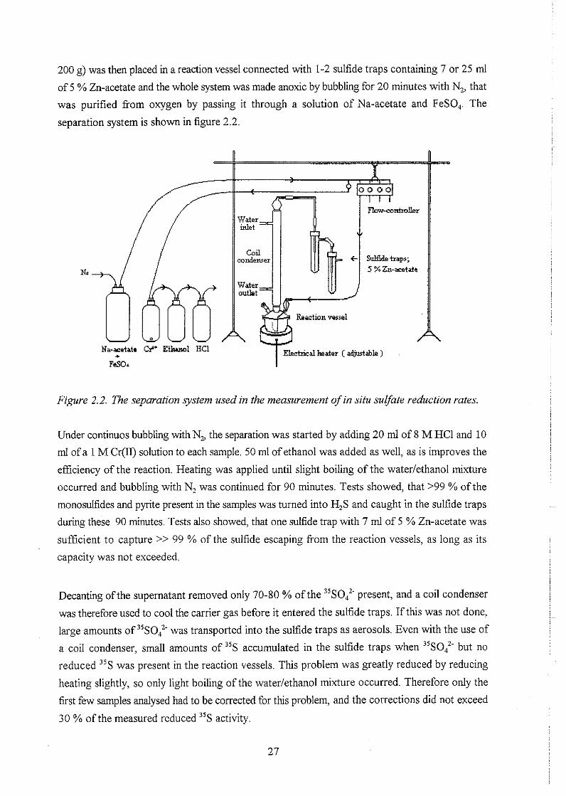
200 g) was then placed in a reaction vessel connected with 1-2 sulfide traps containing 7 or 25 ml
of 5 % Zn-acetate and the whole system was made anoxic by bubbling for 20 minutes with N,, that
was purified from oxygen by passing it through a solution of Na-acetate and FeSO,. The
separation system is shown in figure 2.2.
Figure 2.2. The separation system used in the measurement of in situ suljate reduction rates
Under continuos bubbling withN, the separation was started by adding 20 ml of 8 M HC1 and 10
ml of a 1 M Cr(Q solution to each sample. 50 ml of ethanol was added as well, as is improves the
efficiency of the reaction. Heating was applied until slight boiling of the waterlethanol mixture
occurred and bubbling with N2 was continued for 90 minutes. Tests showed, that >99 % of the
monosulfides and pyrite present in the samples was turned into H,S and caught in the sulfide traps
during these 90 minutes Tests also showed, that one suliide trap with 7 ml of 5 % Zn-acetate was
sufficient to capture >> 99 % of the sulfide escaping from the reaction vessels, as long as its
capacity was not exceeded.
Decanting of the supernatant removed only 70-80 % of the 35S0,2- present, and a coil condenser
was therefore used to cool the carrier gas before it entered the sulfide traps. If this was not done,
large amounts of 35S0,Z- was transported into the sulfide traps as aerosols. Even with the use of
a coil condenser, small amounts of 35S accumulated in the sulfide traps when 35S0,2- but no
reduced 3SS was present in the reaction vessels. This problem was greatly reduced by reducing
heating slightly, so only light boiling of the wateriethanol mixture occurred. Therefore only the
first few samples analysed had to be corrected for this problem, and the corrections did not exceed
30 % ofthe measured reduced 35S activity.
The activity of 3SS was determined on a Wallac 1414 LSC (Liquid Scintillation Counter) by mixing
7 ml ofZn-acetatelsupernatant with 14 ml of Lumagel Safe scintillation liquid (Packard). Quench
corrections were made by external standard, using a quench curve prepared by adding different
amounts of supernatant to samples with known activities of 35S. Colour in the supernatant was the
main quenching factor in these samples. Sulfate concentrations were determined by interpolation
from concentrations measured in water, that was centrifuged out of 2-3 cm long core segments
between the injections points. The sulfate reduction rates were calculated from:
where SRR is the sulfate reduction rate, (SO:) is the sulfate concentration, q,,,,, is the activity
of reduced 35S, anulfvfe is the activity of 35S in the supernatant, t is the incubation time and u is a
fractionation factor.
ol is supposed to correct for the discrimination against heavy isotopes in bacterially mediated
processes. It cannot be determined accurately for natural environments, and a number of different
values can be found in the literature, depending on which strains of sulfate reducers are involved
etc. a was set to 1.06 for sulfate reduction in this study.
The activity of 35S found in the supernatant was used for the rate calculation rather than the
injected activity. The reason for choosing this method was, that some of the tracer might have
been redistributed between the individual samples in each core segment during the incubation
and/or subsequent freezing, and it was assumed to be more correct to use the found 35S activity
for the calculations. The above rate expression is valid, only when the turnover of injected tracer
is low enough to not significantly change the amount of tracer during incubation. Very high
turnovers (up to 80 % in some samples) of35S tracer were observed in samples, where little sulfate
(1-20 pM) was present These high turnovers cannot be assumed to express true in situ rates,
particularly not since the actual sulfate concentration is very inaccurately determined at this low
concentration level For that reason, a cut off level of 15 % turnover of 35S tracer was applied, as
done by (Jakobsen & Postma, 1994; Jakobsen, 1995). All samples, where this level was exceeded,
were discarded from the data. The refinding of "S tracer was 89.6512.5 %. Presumably most of
the lost tracer was situated in the small segments of the core, that were not analysed for 35S.
2.5.3 Methane production and methane oxidation rates
For measurement of methane production and methane oxidation rates, "'CH, had to be separated
from TI1" and 2-14C-acetate. This was done by a two step procedure, where the samples were
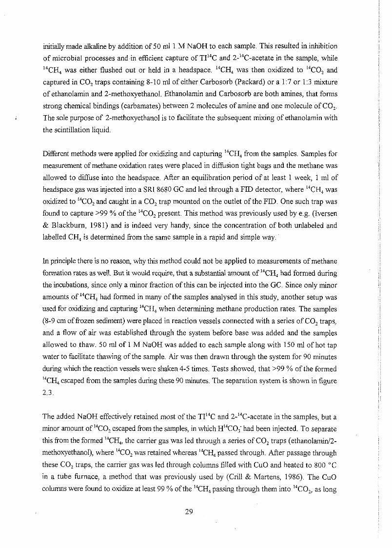
initially made alkaline by addition of SO nll 1 M NaOH to each sample. This resulted in inhibition
of microbial processes and in efficient capture of TII4C and 2-14C-acetate in the sample, while
14CH4 was either flushed out or held in a headspace. 14CH4 was then oxidized to "CO, and
captured in CO, traps containing 8-10 nll of either Carbosorb (Packard) or a 1:7 or 1:3 mixture
of ethanolamin and 2-methoxyethanol. Ethanolamin and Carbosorb are both amines, that forms
strong chemical bindings (carbamates) between 2 molecules of amine and one molecule of CO,.
The sole purpose of 2-methoxyethanol is to facilitate the subsequent mixing of ethanolamin with
the scintillation liquid.
Dierent methods were applied for oxidizing and capturing I4CH4 from the samples. Samples for
measurement of methane oxidation rates were placed in diflksion tight bags and the methane was
allowed to diffuse into the headspace. After an equilibration period of at least 1 week, 1 ml of
headspace gas was injected into a SRI 8680 GC and led through a FID detector, where 14CH4 was
oxidized to I4CO, and caught in a CO, trap mounted on the outlet of the FID. One such trap was
found to capture >99 % of the 14C0, present. This method was previously used by e.g. (Iversen
& Blackburn, 1981) and is indeed very handy, since the concentration of both unlabeled and
labelled CH, is determined from the same sample in a rapid and simple way
In principle there is no reason, why this method could not be applied to measurements of methane
formation rates as weU. But it would require, that a substantial amount of 14CH4 had formed during
the incubations, since only a minor fraction of this can be injected into the GC. Since only minor
amounts of 14CH4 had formed in many of the samples analysed in this study, another setup was
used for oxidizing and capturing I4CH4 when determining methane production rates. The samples
(8-9 cm of frozen sediment) were placed in reaction vessels connected with a series of CO, traps,
and a flow of air was established through the system before base was added and the samples
allowed to thaw. 50 ml of 1 M NaOH was added to each sample along with 150 ml of hot tap
water to facilitate thawing of the sample. Air was then drawn through the system for 90 minutes
during which the reaction vessels were shaken 4-5 times. Tests showed, that >99 % of the formed I4 CH, escaped from the samples during these 90 minutes. The separation system is shown in figure
2.3.
The added NaOH effectively retained most of the TIL4C and 2-I4C-acetate in the samples, but a
minor amount of 14C02 escaped from the samples, in which H14C0,' had been injected. To separate
this from the formed I4CH4, the carrier gas was led through a series of CO, traps (ethanolaminl2-
methoxyethanol), where 14C0, was retained whereas 'TH4 passed through. After passage through
these CO, traps, the carrier gas was led through columns filled with CuO and heated to 800 "C
in a tube furnace, a method that was previously used by (Crill & Martens, 1986). The CuO
columns were found to oxidize at least 99 % ofthe I4CH4 passing through them into 14C0,, as long
as the flow rate was not to high. A column size was chosen (12 mm inner diameter, 25 cm length)
that allowed pumping at the maximum speed of the pump without loss of oxidation efficiency.
L Air inlet Air inlet
Figure 2.3. 7he separation system used in the determination of methane production and methane
oxidation rates. 2-met. stands for 2-methoxyethanol, 1:7 is a I:? mixture of Ethanolamin and
2-methoayethanol, Carb. stands for Carbosorb.
Afler passage of the CuO column, the formed 14C02 was captured in another series of CO, traps.
One CO, trap was enough to capture >>99 % of the 14C02 formed by oxidation of 14CH4.
However, when cleaning traps were used before the oven, some of the ethanolamin and 2-
methoxyethanol in these traps evaporated and was oxidized to H20 and CO, in the oven. Due to
this, the capacity of a single CO, trap was exceeded, and a series of at least two had to be used.
A trap containing 10 ml of 2-methoxyethanol was inserted between the oven and the final CO,
traps to minimize the amount of water entering the CO, traps. This was necessary to avoid phase
separation, when the CO, traps were subsequently mixed with scintillation liquid. The 2-
methoxyethanol traps were regularly checked for I4C content, but only very minor amounts were
found.
The second step of the separation was identical for all 14C samples. The sample was placed in a
reaction vessel connected with a series of CO, traps and made acidic by addition of 30 ml 8 N
HCI. Air was drawn through the system for 90 minutes during which the reaction vessels were
again shaken 4-5 times. Tests showed, that > 99 % of the 14C02 escaped from the reaction vessels
and was caught in the CO, traps during this time. The capacity of CO, traps was adjusted to the
expected carbonate content in the samples, since large amounts of CO, forms from dissolving
carbonate when acid is added to carbonate containing sediment. Again a vial containing 2-
methoxyethanol was inserted before the CO, traps to prevent excessive amounts of water vapour
from entering these CO, traps. Little or no 14C02 was found in these vials with 2-methoxyethanol.
In samples, where 2-"C-acetate was present, a minor amount of this escaped from the reaction
vessels in the second acidic step. Tests showed, that approximately 0.2 % of the 2-14C-acetate
present escaped during a 90 minutes pumping time. For the great majority of samples, this is very
little compared to the amount of 2-"C-acetate, that was turned into TI14C during the incubation.
Moreover, the bulk ofthe 2-'"-acetate, that escaped from the reaction vessels, was caught in the
vial with 2-methoxyethanol, that was inserted to remove water vapour. Therefore the amounts of
2-I4C-acetate entering the CO, traps were very minor. Unreacted 2-14C-acetate was measured in
filtrated supernatant, after both separation steps had been carried out.
AU 14C samples were counted on a Wallac 1414 (July 1997 data) or Packard TRI-CARB - 1600
TR (1996 data) LSC by mixing 8-10 ml of sample with 10 ml of scintillation liquid. Carbosorb was
mixed with Permatlour E, a scintillation cocktail developed by Packard for this purpose. Ethanola-
mid2-methoxy-ethanol was mixed with High Safe scintillation liquids like Ultirna Gold XR
(Packard) or Optiphase HiSafe 3 (Wallac). Supernatant for measuring 2-'"-acetate was mixed
with Lumagel Safe Packard).
Quench corrections were generally made by external standards. At the Packard TRI-CARB - 1600
TR, a quench curve was prepared for the Ethanolamid2-methoxyethanol system by adding
different concentrations of a chemical quenching factor to samples with known activities of '"CO,.
The determination of 2-14C-acetate on the Packard TRI-CARB - 1600 TR was carried out by
internal standards, since colour quench was important in these samples and since a different
scintillation liquid was used. The Wallac 1414 has build in quench libraries, and these gave
satisfying results, except for measurement of 2-"C-acetate in Lumagel Safe. An adjusted quench
curve for this purpose was therefore prepared by adding different concentrations of supernatant
to samples with known activity of 2-14C-acetate.
Many ofthe samples, where HI4COi had been injected, gave such high activities of 14C02 in the
CO, traps during the second separation step, that 14C02 activities exceeded the value (70000 Bq),
where counting is still Linear. This problem, a result of the dead time of the counter, was solved,
either by dilution of the samples, or by correction of the measured '" counts, using a prepared
correction curve.
The methane production rates from October and December 1996 were measured as part of a
M.Sc. thesis by (Nielsen & Holmeijord, 1997). Apparently they had some problems with the
determination of 2-14C-acetate in the December 1996 samples by the internal standard procedure
mentioned above, since the average refinding of tracer was 165 % in these samples. This is
dehitely unrealistic, and the measured amounts of 2-I4C-acetate were therefore adjusted to give
an average refinding of 100 %, before these data were reprinted in this thesis.
As described above, the CH, concentrations, that were used to calculate the methane oxidation
rates, were determined on the SRI 8680 GC, when headspace gas was injected for oxidation and
capturing of I4CH,. This means, that the CH4 concentrations were determined in the samples
themselves. In contrast, the TIC and acetate concentrations, that were used to calculate methane
production rates, were interpolated from nearby water samples.
For determination of TIC this is not a problem, since TIC is present in millimolar concentrations
and therefore practically constant over short vertical distances. Interpolation of the acetate
concentrations &om nearby water samples is far more problematic. As shown in figure 4.10, there
are rather large fluctuations in the measured acetate concentrations over small distances of depth
and between repeated sampling at the same location. Besides this, the turnover of acetate is so
fast, that large diierences in concentration might exist over short vertical and horizontal distances.
To eliminate this problem, it was attempted to measure the acetate concentrations in water from
the sediment cores themselves. Due to problems with high blinds, this was however given up and
the acetate concentrations measured in nearby water samples were used instead. Since fluctuations
and peaks in the acetate concentrations measured in nearby water samples do not necessarily
reflect the concentrations of acetate in the samples used for rate measurement, a smoothing of the
measured concentrations was performed and possibly erratic local peaks in the measured acetate
concentrations were neglected.
This procedure was chosen, because these large peaks in the acetate concentrations gave rise to
large and apparently unrealistic peaks in the measured acetate turnover rates, if they were used.
At location 3 there are rather large deviations between some of the acetate concentrations
measured in June, September and October 1996 (figure 4 10). Since these apparent changes might
not reflect the concentrations in the sediment cores taken in October 1996, the acetate
concentrations at location 3 were calculated from all the values measured in June, September and
October 1996. Due to technical problems, acetate concentrations were not determined at location
3 in July 1997, so the acetate concentrations calculated from the June-October 1996 measurements
had to be used for calculating the July 1997 rates as weU. At location 8 rather large and systematic
variations in the acetate concentrations were found from December 1996 to July 1997 and it was
chosen to calculate the smoothed acetate concentrations at each time separately. The measured
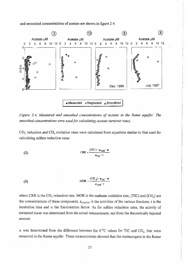
and smoothed concentrations of acetate are shown in figure 2.4.
0 @ @ @ Acetate pM Acetate pM Acetate IJM Acetate pM
0 2 4 6 8 1 0 1 2 0 2 4 6 8 3 0 1 2 0 2 4 6 8 1 0 1 2 0 2 4 6 8 1 0 1 2 0
2
4 0 4 E
6
8
Figure 2.4. Measured and smoothed concentrations of acetate in the Rsm0 aquifer. The
smoothed concentrations were used for calculating acetate turnover rates.
CO, reduction and CH, oxidation rates were calculated from equations similar to that used for
calculating sulfate reduction rates:
(CH,, . a,. u MOR -
CHI' '
where CRR is the CO, reduction rate, MOR is the methane oxidation rate, (TIC) and (CH,) are
the concentrations of these compounds, a,,,,, is the activities of the various fractions, t is the
incubation time and a the fractionation factor. As for sulfate reduction rates, the activity of
umeacted tracer was determined from the actual measurement, not from the theoretically injected
amount.
a was determined from the difference between the 613C values for TIC and CH,, that were
measured in the Rsms aquifer. These measurements showed that the methanogens in the RQms
aquifer have a fractionation factor between "C and IZC of 1.04-1.06. It is usually assumed, that
the fractionation between 'T and I2C is twice as large as that between I3C and "C, and a was
therefore conservatively set to 1.08 for methane production. Slightly higher fractionation factors
are usually reported for CO, reduction than for acetate fermentation (Whiticar & Faber, 1986),
so perhaps a slightly higher value could have been justified for CO, reduction. But given the many
other uncertainties involved in these measurements and the large variability in the rates (figure
4.16), an exact determination of a is unimportant for the scope of this study. For CH4 oxidation
much smaller fractionation factors are reported (Whiticar et al. 1986), and these values are highly
uncertain. Accordingly no attempt was made to correct the measured CH, oxidation rates for
isotopic fractionation and a was set to 1.00 for methane oxidation.
The equation used for calculating acetate turnover rates is slightly more complicated, as a large
fiaction of the injected tracer is turned over during the incubation period. 25-50 % turnover of the
acetate tracer was often observed, and in one sample as much as 92.5 % of the tracer was turned
over. This means, that it cannot be assumed, that the concentrations of 2-14C-acetate in the
samples were constant during the incubations. It is therefore necessary to use a rate expression,
where an exponential decrease in the concentration of unreacted tracer over time is assumed, as
would be the case, if the rates and unlabeled acetate concentrations were constant over time.
Accordingly the acetate turnover rates (ATR) were calculated from:
Am- B . (acetate ) + "TIC * ' C H ~ .In t "=MI
where (acetate) is the concentration of acetate, a,4mCia,,, is the activities measured in the various
fractions, u is the fractionation factor (1.08) and t is the incubation time.
The acetate fermentation rates (AFR) and acetate oxidation rates (AOR) were calculated from:
AFR - ATR . " C H ~
' C H ~ * ' 7 7 ~
AOR - ATR . "TIC
'CHI "TIC
using the acetate turnover rate calculated from (4).
34

The refinding of tracer was 90.2*8.6 % for 2-14C-acetate and 94.2*7.6 % for '4C02. As for
measurement of sulfate reduction rates, most of the lost tracer was presumably located in the small
sections of the core, that were not analysed for 14C. For the 14CH4 tracer, the average refinding
cannot be determined meaningfully, since loss of activity from the standard occurred during field
work. Moreover, the amount of '*CH4 found in each sample varied highly. Since the refinding of
unlabeled methane in the samples was -100 % based on a comparison between methane
concentrations measured in the rate samples and in water samples from the same spot, this can
only be because large and highly variable losses of 14CH4 tracer occurred during the injections.
Alternatively large and highly variable amounts of "CH, should have been lost between the FID
detector and the CO, traps mounted on the FID outlet. However, tests showed, that this was not
the case. The large and highly variable loss of '"H, tracer presumably happened, because this
tracer was on gas form, whereas the other tracers were dissolved in water. The use of a dissolved
CH, tracer in future studies is therefore recommended.
In principle it is not a problem for the rate measurement, that the amount of tracer varies highly,
as long as the rate is calculated from the actually found amount of tracer, and the injected amount
of tracer is low enough to not affect the rates. In this case however, the amount of reaction
product formed was so low, that the detection l i t of the method was not reached in many
samples. In figure 2.5 is shown a comparison between the amounts of I4CH, and 14C0, found in
samples, where methane oxidation rates were measured.
At location 3 and 10, most of the samples contained less than 20 DPM 14COZ. These low activities
give rise to large uncertainty in the LSC process, but worse is, that the correlation between 14C02
and 14CH4 is week (R2= 0.161 at location 3) or completely absent (R2 = 0.020 at location 10) and
that the intercepts of the linear regressions are far from zero. This strongly indicates, that the
measurements of 14C02 are subject to systematic errors. At location 8 higher amounts of 'TO,
were found in most samples, but the correlation between 14C02 and 'TH, is still not good (R2 =
0.140) and the regression line at location 8 has an intercept of 22k18 DPM, whereas the similar
values are only 5 * 3 DPM at location 3 and 9 * 6 DPM at location 10. Apparently the higher
"CO, activities found at location 8 are not completely related to turnover of the injected tracer
either.
A closer inspection of the measurements from location 8 reveals, that all the correlation between
'"H, and 14COZ comes from samples above 3 m.b.s. When the data from location 8 are split up
at this depth, the resulting correlations are R2= 0.381 above 3 m.b.s. and only RZ = 0.012 below
3 m.b.s. Also the intercept of the regression line is lower for the samples above 3 m.b.s. (16k21
DPM) than for those below 3 m.b.s. (28i15 DPM). In conclusion reliable estimates of methane
oxidation rates have only been obtained above 3 m.b.s. at location 8. At larger depths at location
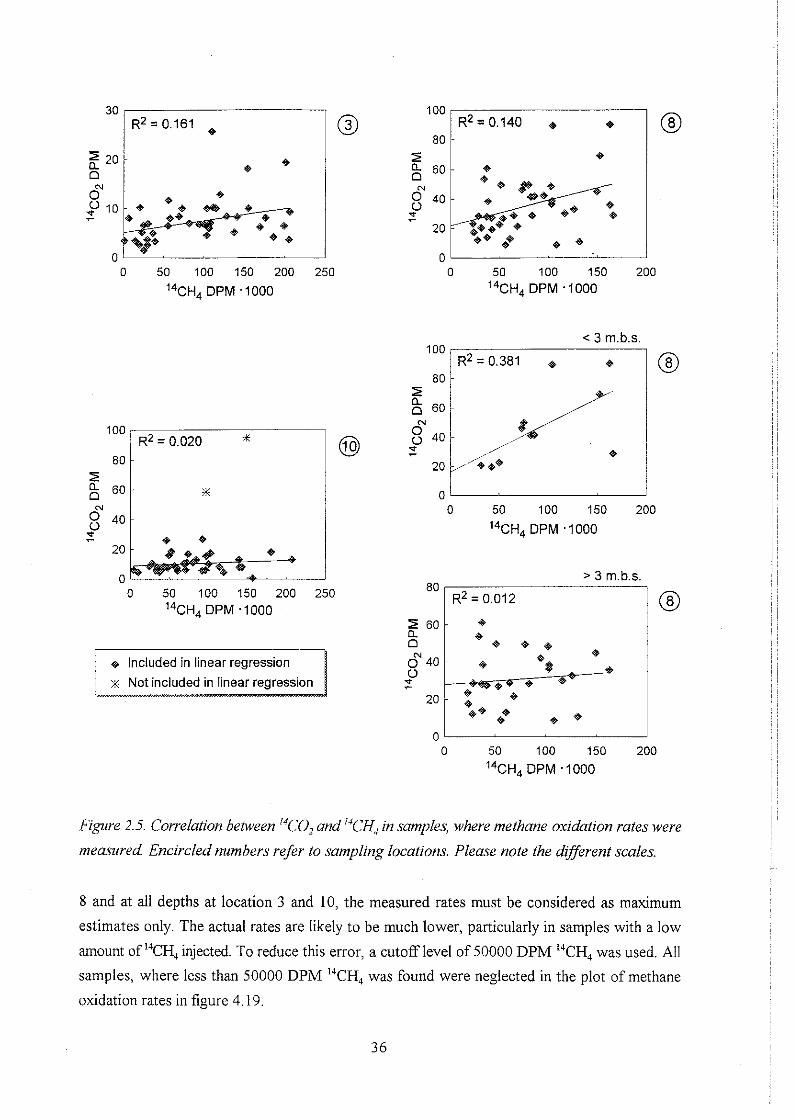
0 50 100 150 200 250
I4cH4 DPM .I000
0 50 100 150 200 250 i 4 ~ ~ 4 DPM ,1000
0 50 100 150 200 j4cH4 DPM . lo00
0 50 100 150 200
I4cH4 DPM ,1000
" 0 50 100 150 200
' 4 ~ ~ , DPM .I000
Figure 2.5. Correlation between 14C0, andM(:H4 in samples, where methane oxidation rates were
measured Encircled numbers refer to sampling locations. Please note the dijferent scales.
8 and at all depths at location 3 and 10, the measured rates must be considered as maximum
estimates only. The actual rates are likely to be much lower, particularly in samples with a low
amount of "CH, injected. To reduce this error, a cutoff level of 50000 DPM 14CH4 was used. All
samples, where less than 50000 DPM 14CH4 was found were neglected in the plot of methane
oxidation rates in figure 4.19.
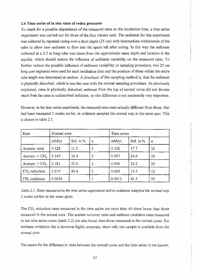
2.6 Time series of in situ rates of redox processes
To check for a possible dependence of the measured rates on the incubation time, a time series
experiment was carried out for three of the four tracers used. The sediment for this experiment
was collected by repeated coring over a short depth (25 cm) with intermediate withdrawals of the
tube to allow new sediment to flow into the space left after coring. In this way the sediment
collected in a 2.5 m long tube was taken from the approximate same depth and location in the
aquifer, which should reduce the influence of sediment variability on the measured rates. To
further reduce the possible influence of sediment variability or sampling procedure, two 25 cm
long core segments were used for each incubation time and the position of these within the entire
tube length was determined at random. A drawback of this sampling method is, that the sediment
is physically disturbed, which is less the case with the normal sampling procedure. As previously
explained, rates in physically disturbed sediment from the top of normal cores did not deviate
much from the rates in undisturbed sediment, so this difference is not necessarily very important.
However, in the time series experiment, the measured rates were actually different from those, that
had been measured 2 weeks earlier, in sediment sampled the normal way at the same spot. This
is shown in table 2.1.
Table 2. I . Rates measured in the time series experiment and in sediment sampled the normal way
2 weeks earlier at the same spots.
The CO, reduction rates measured in the time series are more than 40 times lower than those
measured in the normal core. The acetate turnover rates and methane oxidation rates measured
in the time series cores (table 2.2) are also lower than those measured in the normal cores. For
methane oxidation this is however highly uncertain, since only one sample is available from the
normal core.
The reason for the difference in rates between the normal cores and the time series is not known.
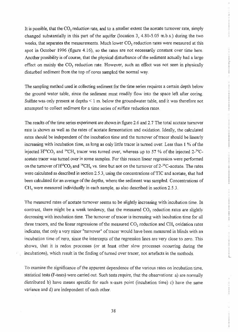
It is possible, that the C02 reduction rate, and to a smaller extent the acetate turnover rate, simply
changed substantially in this part of the aquifer (location 3, 4.80-5.05 m.b.s.) during the two
weeks, that separates the measurements. Much lower CO, reduction rates were measured at this
spot in October 1996 (figure 4.16), so the rates are not necessarily constant over time here.
Another possibiity is of course, that the physical disturbance of the sediment actually had a large
effect on mainly the CO, reduction rate. However, such an effect was not seen in physically
disturbed sediment from the top of cores sampled the normal way.
The sampling method used in collecting sediment for the time series requires a certain depth below
the ground water table, since the sediment must readily flow into the space left after coring.
Sulfate was only present at depths < 1 m. below the groundwater table, and it was therefore not
attempted to collect sediment for a time series of sulfate reduction rates.
The results of the time series experiment are shown in figure 2.6 and 2.7 The total acetate turnover
rate is shown as well as the rates of acetate fermentation and oxidation. Ideally, the calculated
rates should be independent of the incubation time and the turnover of tracer should be linearly
increasing with incubation time, as long as only little tracer is turned over. Less than 1 % of the
injected H14C0, and "CH, tracer was turned over, whereas up to 57 % of the injected 2-14C-
acetate tracer was turned over in some samples. For this reason linear regression were performed
on the turnover ofH14C0, and I4CH4 vs. time but not on the turnover of 2-14C-acetate. The rates
were calculated as described in section 2.5.3, using the concentrations of TIC and acetate, that had
been calculated for an average of the depths, where the sediment was sampled. Concentrations of
CH, were measured individually in each sample, as also described in section 2.53.
The measured rates of acetate turnover seems to be slightly increasing with incubation time In
contrast, there might be a weak tendency, that the measured CO, reduction rates are slightly
decreasing with incubation time. The turnover of tracer is increasing with incubation time for all
three tracers, and the linear regressions of the measured CO, reduction and CH, oxidation rates
indicates, that only a very minor "turnover" of tracer would have been measured in blinds with an
incubation time of zero, since the intercepts of the regression lines are very close to zero. This
shows, that it is redox processes (or at least other slow processes occurring during the
incubations), which result in the finding of turned over tracer, not artefacts in the methods.
To examine the significance of the apparent dependence of the various rates on incubation time,
statistical tests (F-tests) were carried out. Such tests require, that the observations. a) are normally
distributed b) have means specific for each x-axes point (incubation time) c) have the same
variance and d) are independent of each other
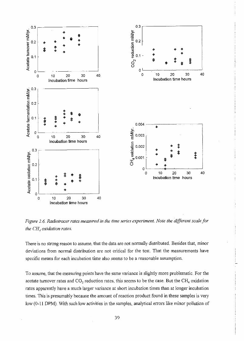
.
0 10 20 30 40. lncubation time hours
o 1 I
0 10 20 30 40 lncubation time hours
10 20 30 lncubation time hours
0 10 20 30 40 lncubation time hours
"
0 10 20 30 40 lncubation time hours
Fzgure 2.6. Radiotracer rates mewired in the time series experiment. Note the different scale for
the CH, oxidation rates.
There is no strong reason to assume, that the data are not normally distributed. Besides that, minor
deviations from normal distribution are not critical for the test. That the measurements have
specific means for each incubation time also seems to be a reasonable assumption.
To assume, that the measuring points have the same variance is slightly more problematic. For the
acetate turnover rates and CO, reduction rates, this seems to be the case. But the CH, oxidation
rates apparently have a much larger variance at short incubation times than at longer incubation
t i e s . This is presumably because the amount of reaction product found in these samples is very
low (0-1 1 DPW. With such low activities in the samples, analytical errors like minor pollution of
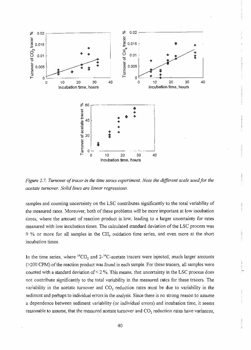
0 10 20 30 40 0 10 20 30 40 Incubation time, hours Incubation time, hours
- I- 0 10 20 30 40
lncubation time, hours
Figure 2.7. Turnover of tracer in the time series experiment. Note the dijferent scale used for the
acetate turnover. Solid lines are linear regressions.
samples and counting uncertainty on the LSC contributes significantly to the total variability of
the measured rates. Moreover, both of these problems will be more important at low incubation
times, where the amount of reaction product is low, leading to a larger uncertainty for rates
measured with low incubation times. The calculated standard deviation of the LSC process was
9 % or more for all samples in the CH, oxidation time series, and even more at the short
incubation times.
In the time series, where 14C02 and 2-"C-acetate tracers were injected, much larger amounts
(>ZOO CPM) of the reaction product was found in each sample For these tracers, all samples were
counted with a standard deviation of < 2 %. This means, that uncertainty in the LSC process does
not contribute significantly to the total variability in the measured rates for these tracers. The
variability in the acetate turnover and CO, reduction rates must be due to variability in the
sediment and perhaps to individual errors in the analysis. Since there is no strong reason to assume
a dependence between sediment variability (or individual errors) and incubation time, it seems
reasonable to assume, that the measured acetate turnover and CO, reduction rates have variances,
that are independent of the incubation time.
Assuming that the measured rates are independent of each other is again slightly problematic, since
two measuring points with the same incubation time are always located next to each other. To
examine the possible influence of this, the measured rates were plotted against the location of the
samples in the core, indicated by a number fiom 1-20. Sample 1-2 are from the lowest 25 cm core
segment (the last sediment sampled), etc. For acetate the total turnover rate is shown as well as
the rates of acetate oxidation (to COJ and fermentation (to CH,). This plot is shown in figure 2.8.
"
0 5 10 15 20 Sample nr.
Sample nr.
0 5 10 15 20 Sample nr.
I
0 10 20 Sample nr.
- 0 5 10 15 20
sample nr.
Figure 2.8. Radiotvacer rates meastrred in the time series experiment as function of the position
of samples within the sampling tube. Fzrrther details arefozmd in the text.
There does not seem to be any systematic variation between the measured acetate turnover rates
and the location of samples within the core. On the other hand, there seems to be some systematic
variations in the C 0 2 reduction rates. There are two distinct parts of the CO, reduction core
(sample 1-3 and 10-1 l), where the rates appears to be significantly higher than in the rest of the
core.
Run tests were performed to investigate whether it could be assumed, that the measured rates
were independent of their location within the sampling tube. This was done by finding the median
rate in each set of data and asserting all samples with a higher rate with an "a" and all samples with
a lower rate with a "b". The number of runs ( e.g. aaiblaaaibb etc.) were then counted. For CO,
reduction the same test was performed, using a rate of 0.1 rnM1yr as the dividing point. This was
done to test, if the distribution of the 5 samples with rates higher than this could be assumed to
be a coincidence. Since this was rejected on a 95 % level, it was assumed, that these five samples
actually belonged to a diierent population and accordingly they were removed from the data and
a new test was performed on the remaining 12 samples. Why the rates are higher in these two
parts of the CO, reduction core is unknown, but it could be due to a few occasions, where the
sampling tube was unintentionally driven about 20 cm further than planned. The sediment thus
sampled from slightly larger depths might have higher CO, reduction rates than the rest The
results of the Run tests are shown in table 2.2.
Table 2.2. Run tests for examining the possible dependence of radiotracer rates on position in
the sampling tubes in the time series experiment. The hypothesis of independence between
measured rates andposition in the core is rejected in the critical area.
The hypothesis, that the measured rates are independent of the location within the sampling tube,
cannot be rejected on a 95 % level for any of the acetate rates. Moreover, the number of runs are
well within the h t s given by the test, indicating that it is very reasonable to assume, that highilow
values of the acetate turnover rates are randomly distributed over the tube length. For the CO,
reduction rates, independence can not be rejected on a 95 % level, when the testing is done using
the median rate to divide the data. But it can be rejected on a 80 % level. And if a value of 0.1
mWyr. is used for dividing the data rather than the median, the hypothesis is rejected on a 95 %
level. This indicates, that the five samples with rates higher than 0.1 N y r . are not randomly
distributed over the tube length. If these five samples are taken out, there is no indication at all,
that the remaining 12 samples have rates, that are not randomly distributed over the tube length.
For the CH, oxidation rates, the hypothesis of random distribution of higWlow rates over the tube
length is rejected, mainly because most of the low rates are measured in the bottom of the core
(low numbers) and vice versa. The reason for this is unknown, but perhaps the sediment very close
to the sampling position had higher CH, oxidation rates than the surrounding sediment. It is
noteworthy, that the CH, oxidation rates forms a relatively smooth curve when plotted against
location in the sampling tube, whereas they vary highly when plotted against the incubation time.
This indicates, that some of the apparently systematic variations in the measured CH, oxidation
rates at different incubation times, e.g. the low rates at 13.5 hours, are mainly the result of the
different location of samples within the sampling tube.
In conclusion the requirements of the validity of an F-test is met by the acetate tumover rates and
CO, reduction rates (the 12 samples with rates < 0.1 N y r ) , but not by the methane oxidation
rates. However, a visual inspection of the CH, oxidation rates does not disclose any systematic
dependence on the incubation time, so most likely such a dependence is small or non existent.
To test, whether the acetate turnover and CO, reduction rates are independent of the incubation
t i e , it fust has to be tested, whether there is a linear dependence between the measured rates and
the incubation time This cannot be rejected on testing levels of 50 % or higher for any of the
acetate rates or for the CO, reduction rates. Having clarified this, we can now test, again using an
F test, whether it can be assumed, that the measured rates are independent of the incubation time
(i.e. the slope of the line is 0). This cannot be rejected for the CO, reduction rates on testing levels
of 50 % or higher. But for the acetate turnover rates, this hypothesis is rejected on testing levels
as high as 90 % (acetate oxidation), 95 % (acetate fermentation) and 99.5 % (total acetate
turnover). This means, that there is no indication of any dependence between the measured CO,
reduction rates and incubation times, but a strong indication for such a dependence between the
measured acetate turnover rates and incubation time.
The time dependence is not particularly large however. The linear regression of the acetate
turnover rates indicate, that 1917 % higher acetate turnover rates would have been measured, if
an incubation time of 24 hours (as for the other tracers) had been used instead of 12 hours. This
value is highly uncertain and it is unknown whether the rates measured at high or low incubation
times are most correct. It is also unknown whether the effect of incubation time would be similar
on sediment sampled the normal way or from other locations and depths in the aquifer. It was
therefore not attempted to correct the measured acetate turnover rates for the apparent time
dependence. But it would be relevant to investigate this subject further before more rate
measurements are made with the method described here.
Perhaps the production of acetate was stalled by the disturbance of sediment during sampling and
the concentration of unlabelled acetate decreased with time at a rate similar to the decrease in the
concentration of 2-lJC-acetate. If the rate is unaffected by minor changes in the acetate
concentration, then the turnover of 2-14C-acetate should be almost linear with time, which indeed
seems to be the case (figure 2.7). If the sampling procedure used in the time series experiment
disturbed the fermentation of organic matter, it would be expected, that the production of H,
decreased along with the production of acetate. This might be the explanation for the large
decrease in the CO, reduction rate compared to sediment, sampled the normal way, two weeks
earlier, at the same spot. If this is the case, the time dependency problem does probably not exist
in sediment sampled the normal way.
It is also possible however, that the time dependency has other reasons. One such reason could
be a large increase in the acetate concentration near the line of injection, where most of the tracer
is present shortly after injection. As previously mentioned, the increase in acetate concentration
was < 1 %, ifit is assumed, that the tracer is distributed equally over the entire sample. However,
the tracer is not equally distributed, particularly not shortly after injection. If a small increase in
the acetate concentration has little or no effect on the acetate turnover rate, the actual rate will be
underestimated due to the artificially increased acetate concentration. This effect will decrease
with time because of diffusion and turnover of the injected tracer, and could therefore be
responsible for the observed time dependence. If this is the case, the problem can be solved by
injecting less tracer and/or by applying a longer incubation time. The latter would however not be
practical in the few samples, where a turnover time of acetate down to 5 hours was found (figure
5.4).
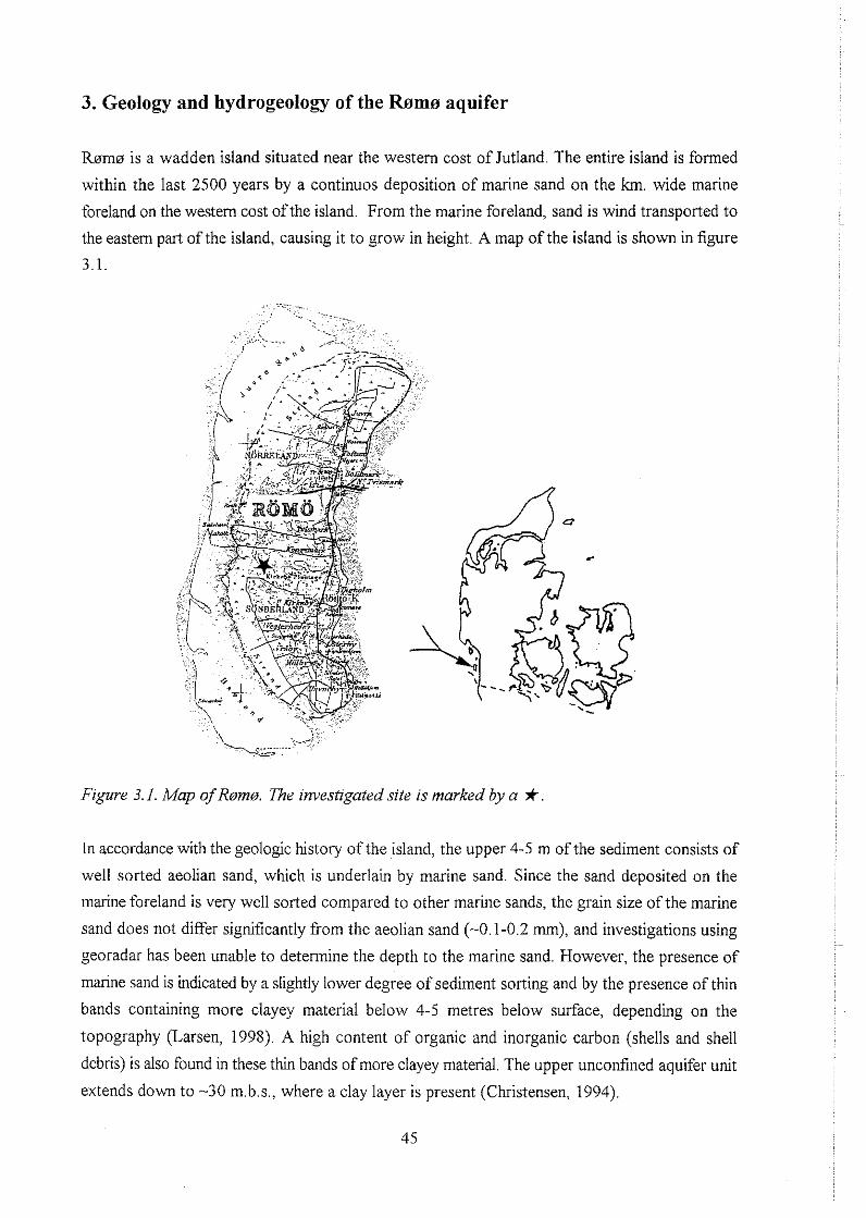
3. Geology and hydrogeology of the Rsms aquifer
Rsm0 is a wadden island situated near the western cost of Jutland. The entire island is formed
within the last 2500 years by a continuos deposition of marine sand on the km. wide marine
foreland on the western cost ofthe island. From the marine foreland, sand is wind transported to
the eastern pa^? of the island, causing it to grow in height. A map of the island is shown in figure
3.1.
Figure 3. I . Map of R0m0. The investigated site is marked by a A-
In accordance with the geologic history of the island, the upper 4-5 m of the sediment consists of
well sorted aeolian sand, which is underlain by marine sand. Since the sand deposited on the
marine foreland is very well sorted compared to other marine sands, the grain size of the marine
sand does not differ significantly from the aeolian sand (-0.1-0.2 rnm), and investigations using
georadar has been unable to determine the depth to the marine sand. However, the presence of
marine sand is indicated by a slightly lower degree of sediment sorting and by the presence of thin
bands containing more clayey material below 4-5 metres below surface, depending on the
topography (Larsen, 1998). A high content of organic and inorganic carbon (shells and shell
debris) is also found in these thin bands of more clayey material. The upper unconfined aquifer unit
extends down to -30 m.b.s., where a clay layer is present (Christensen, 1994).
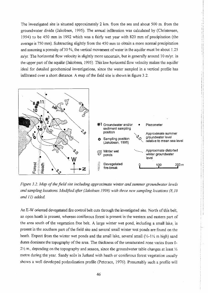
The investigated site is situated approximately 2 km. from the sea and about 500 m. from the
groundwater divide (Jakobsen, 1995). The annual infiltration was calculated by (Christensen,
1994) to be 450 mm in 1992 which was a fairly wet year with 820 mm of precipitation (the
average is 750 mm). Subtracting slightly from the 450 mm to obtain a more normal precipitation
and assuming a porosity of 30 %, the vertical movement ofwater in the aquifer must be about 1.25
mlyr The horizontal flow velocity is slightly more uncertain, but is generally around 10 d y r . in
the upper part of the aquifer (Jakobsen, 1995). This low horizontal flow velocity makes the aquifer
ideal for detailed geochemical investigations, since the water sampled in a vertical profile has
infiltrated over a short distance. A map of the field site is shown in figure 3.2.
@I1 Groundwater andlor sediment sampling position
0 Sampling position (Jakobsen, 1995)
g Whnter wet ponds
.:$ Devegetated fire-break
Piezometer
\ Approximate summer groundwater level
\ relat~ve to mean sea level
- - Approximate distorted winter groundwater level
Figure 3.2. Map of the field site including approximate winter and summer groundwater levels
and smpling locations. ModEfied 4 e r (Jakobsen 1998) with three new sampling locations (8, f 0
and I I ) added.
An E-W oriented devegetated h e control belt cuts through the investigated site. North of this belt,
an open heath is present, whereas coniferous forest is present in the western and eastern part of
the area south of the vegetation free belt. A large winter wet pond, including a small lake, is
present in the southern part of the field site and several small winter wet ponds are found on the
heath. Expect from the winter wet ponds and the small lake, several small (%-I% m high) sand
dunes dominate the topography of the area. The thickness of the unsaturated zone varies from O-
2% m., depending on the topography and season, since the groundwater table changes at least %
metre during the year. Sandy soils in Jutland with heath or coniferous forest vegetation usually
shows a well developed podzolization profile (Petersen, 1976). Presumably such a profile will
eventually be formed on b n w too, but due to the young age of the Island, no clear podzolization
profile exists yet.
The general flow direction in the aquifer is SE-NV (figure 3.2). However the large winter wet
pond in the southern part of the area causes a seasonal change in the flow direction in parts of the
aquifer, most profoundly near location 3, that is situated very close to the winter wet pond. The
flow velocity at location 3 is also higher during the winter as indicates to the close lying equi
potential lines in the winter situation.
Detailed geochemical studies have been carried out by (Jakobsen & Postma, 1994; Jakobsen,
1995; Larsen, 1998) at location 1-6. However, at the time of this investigation, methane was only
found at location 3, and accordingly three new sampling locations (8,lO and 1 I), all situated along
a flow line in the western part of the area (figure 3.2), were chosen for the investigation along with
location 3. Location 10 is situated on the top of a 1-1% m high sand dune, and the distance to the
groundwater table is 1-1% m larger than at the other locations. To enable a better comparison of
the results from the various sampling locations, all depths are shown relative to a fixpoint at
location 3. The term "x m.b.s." means, that the sample was taken x metres below a level, that
corresponds to the terrain at location 3. Since the water table only differed by 9 cm between the
sampled locations in July 1997, the corrected depths are also comparable with respect to the
groundwater table. The groundwater table is not shown in the figures, because it varies at least
!h metre during the year, but the upper samples shown are generally not more than % m. below
the groundwater table at the time of sampling, sometimes even much less.
4. Results
4.1 General water chemistry
The general water chemistry in the Rsw aquifer was described by (Jakobsen, 1995), who found
large variations between the 5 sampled locations. As there might also be temporal variations,
location 3 was resampled for this investigation together with the new locations 8 and 10 (figure
3.2). A cumulative plot of the major cations and anions at the various locations is shown in figure
4.1.
The total solute concentration varies from 3-7 meqll at the three sampling locations. The general
concentration level of C1- is - 2 mM at all locations. In 1996 elevated C1- concentrations of up to
4 mM were found at location 8 from 1.4 to 2.4 m.b.s.. These elevated C1- concentrations are
probably the result of dry deposition of sea salt during winter storms at location 8, which is
situated at the edge of the forest. At location 10, situated just 13 m upstream from location 8, but
behind the forest edge, elevated C1- concentrations were not found in 1996.
To check for temporal variations in the general water chemistry, location 3 was resampled for all
major ions in September 1996, four months after the initial sampling. In July 1997, all locations
were resampled for CI'. The results are shown in figure 4.2.
The general water chemistry did not change much at location 3 fiom May to September 1996. The
only major ion, that show some general change in concentration, is Na'. This is somewhat
puzzling, since the concentrations of C1- and all other major ions remained practically constant. A
closer inspection reveals a considerable covariation between the changes in Na'concentration and
the changes in deviation from electro neutrality from May to September (data not shown).
Accordingly, erroneous measurements of Na' is the most likely explanation for the apparent
change in Na' concentration from May to September 1996. The high concentrations of CI, Na'
and Mg2' in the upper sample from September 1996 are probably a result of evaporation due to
a falling groundwater table during the summer, where little or no infiltration occurred.
A large peak exists in the concentrations of K' and Mg2' at location 3, at appr. 6 m.b.s. The reason
for this is not known, but it could be a result of ion exchange reactions following from a past salt
pulse passing through this part of the aquifer. The repeated measurement of C1- concentrations in
July 1997 revealed no major changes in the deeper parts of the aquifer. But at location 10 a salt
peak infiltrated the aquifer during the winter of 1996-1997, raising the concentration of C1- from
2 - 3.5 rnM above 2 m.b.s. At location 3 and 8, the CI- concentration remained relatively constant
from 1996 to July 1997 except for a narrow peak at location 8, 2 m.b.s.

Anions meqll. Cations meqll. -8 -6 -4 -2 0 0 2 4 6 8
Figure 4 I : Cumulative plots of major cations and nnions in the Ram0 aquifer. The samples were
taken in Mq 1996 (locaiion 3) and December 1996 (location 10 and 8). Encircled numbers refer
to sampling locations.
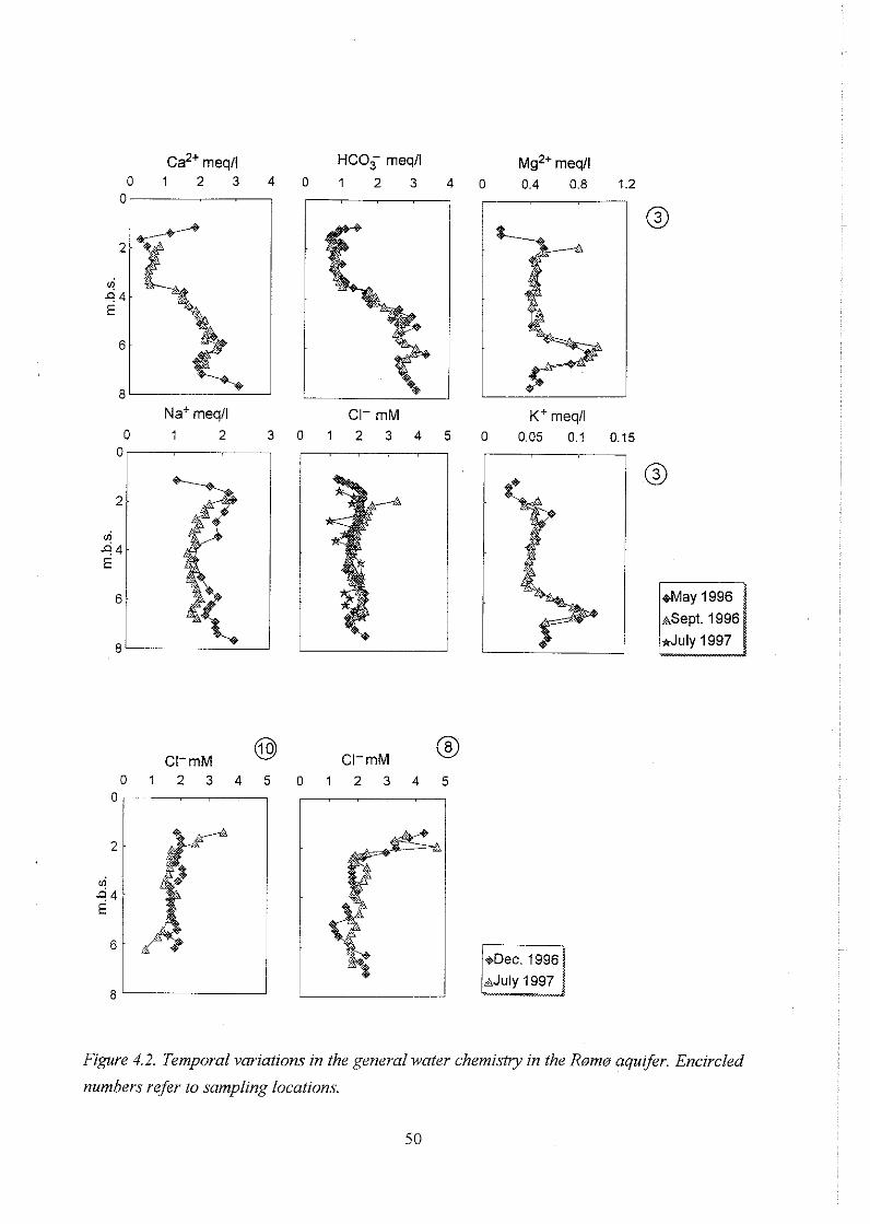
ca2+ rneqll HC03 rneqll ~ g ~ + meqll 0 1 2 3 4 0 1 2 3 4 0 0.4 0.8 1.2
Na+ rneqll
0 1 2 3 CI- rnM
0 1 2 3 4 5 - K+ rneqll
0 0.05 0.1 0.15
Figure 4.2. Temporal variations in the general water chemistry in the Ram0 aquifer. Encircled
numbers refer to sampling locations.
The water chemistry shows a clear influence of Ca-carbonate dissolution (figure 4.3). The Ca2+
concentration increase sharply at a certain depth at all three locations, and then continues to
increase slowly with depth, until equilibrium with calcite is approached in the deeper parts of the
aquifer. At location 3 and 10, the increase in Ca2' concentration is accompanied by an increase in
pH from 6.2-6.5 to 7.3-7.5 at the same depths where the Ca2+ concentration starts to increase.
ALkahity also increases at location 3 and 10 at the same depths as Ca2+ and pH, exactly as would
be expected, if calcite dissolution occur according to (7).
Most of the Ca-carbonates in the Rarms aquifer are shells and shell fragments of mussels.
Accordingly, calcite is probably not a realistic representative of the Ca-carbonates, but this is
unimportant for the scope of this study. What is important is, that the pH, alkalinity and Ca2+
concentration in parts of the aquifer is controlled by dissolution of Ca-carbonates.
At location 8 the concentration of calcium was high (2 meq/l) above 2 m.b.s. in December 1996,
then decreased sharply around 2 m.b.s and increased sharply again around 3 m.b.s. This most likely
reflects an inhomogeneous distribution of shell fragments in the sediment shortly upstream from
location 8. Location 8 is situated downstream a large sand dune, where large amounts of shell
fragments might have been wind deposited. The generally much lower alkalinity above 3 m.b.s.
at location 8 in July 1997 (figure 4.3) suggests that less Ca-carbonate had been dissolved in the
water found here in July 1997. So apparently the dissolution of calcite vary highly along slightly
different flow paths in this part of the aquifer. In accordance with the distribution over depth of
Ca2+, pH and alkalinity is also higher in the upper part of the aquifer at location 8 than at the other
two locations. This, however, is also likely to be the result of Fe(II1)-oxide reduction, as will be
shown in the next section.
The SI (Saturation Index) for calcite and the alkalinity in July 1997, both shown in figure 4.3, was
calculated with PHREEQC (Parkhurst & Appelo, 1997) entering values of pH, TIC, SO:- and
Fez' measured in July 1997 and concentrations of all other cations (including Ca2+) measured in
SeptemberIDecember 1996. C1' concentrations were adjusted to achieve electro neutrality and
depths were adjusted to each other by interpolation of the 1996 data. This less than ideal
procedure was necessary, because no complete water analysis were available, where all
components had been determined at the same time.
Gven the large deviation between the alkalinity 1.5-2.7 m.b.s. at location 8 in December 1996 and
July 1997, it is reasonable to assume, that SIC,,,,,, also changed substantially here between these
Alkalinity meqll. ca2+ meqll PH Log ( lAPlKcalcite) 0 1 2 3 4 0 1 2 3 4 5 6 7 8 -5 -4 -3 -2 -1 0
Figure 1.3. Carhonate chemistry at three sampling locations (encircled numbers) in the R~rn@
nquijer. Details on the calczilatior~s are found in the text.
two sampling times. Si,,, was probably higher than shown
in December 1996 and lower than shown in July 1997 in this SIC rnrnollkg dly wt, . .
part of the aquifer. It is even possible, that saturation for o 100 ZOO 300 0
calcite was approximated in December 1996. At larger
depths and at the other two locations, the alkalinity changed 2
only slightly &om 1996 to 1997. This makes it unlikely, that
SICaicit, changed substantially here from 1996 to 1997, and 9 $ 4
the calculated SIC,,,, is probably representative for both E
sampling times. 6
At location 3 the SIC (Sedimentary Inorganic Carbon) 8-
content in the sediment was determined along with the
determination of SOC (Sedimentary Organic Carbon). The Figure 4.4. SIC content in the sediment at location 3 in the Rsmo
results are shown in Figure 4.4 and agree well with the aquifer, "
measured water chemistry No or little SIC is present in the
sediment at location 3 above the depth (4 m.b.s.), where pH increases along with the Ca2+
concentration and alkalinity.
4.2 Redox chemistry
4.2.1 Redox sensitive solutes
The simplest method to determine the redox conditions in sediments is to look at the disappearan-
ce of substances being reduced, e.g. 0, NO,' or SO:., and at the appearance of reaction products
like CH,, Fe2', iVn2' or H2S. Unfortunately the picture might be disturbed by further reaction of
the reaction products. H2S produced by sulfate reduction might precipitate as FeS or FeS,, if
dissolved Fe2' or reactive Fe(II1)-oxides are available. Fez', formed by Fe(II1)-oxide reduction,
might precipitate not only as FeS or FeS,, but also as siderite (FeCO,). Since the activity of CO?.
is strongly dependent on pH, the latter reaction is mainly seen at high or neutral pH values.
Saturation calculations showed that Siderite is a realistic phase in the h m a aquifer. The
concentration of dissolved Fe2" is also subject to ion exchange reactions with the sediment and to
sorption to organic matter. Finally CH, might be reoxidized to HCOi or transported upwards as
bubbles, if the water gets supersaturated with dissolved gasses. Also, temporal changes in the
composition of the d t r a t i n g water, along with horizontal differences in the sediment, will affect
the water composition along the different flow lines intersected by a vertical concentration depth
profile. This might lead to false conclusions, if concentration gradients alone are used to estimate
rates of redox processes.
Yet, while this simple method is far from perfect, it is still a feasible one for getting a rough
overview of the redox processes occurring in an aquifer. Concentrations of O2 and NO; are
always below the detection limit in the b m aquifer, even in samples taken just 10-20 cm. below
the groundwater table. HzS concentrations are also generally below the detection limit (1 pM),
presumably because there is always enough dissolved Fe2' in the water to cause precipitation of
FeS or FeS,. The most relevant redox sensitive solutes to look at in the Rprm aquifer are
therefore: Md', Fez', SO:. and CH,. Concentration depth profiles of these solutes are shown in
figure 4.5.
Judging from the concentration depth profiles for Mn2', the reduction of Mn(1V)-oxides is only
of any quantitative importance at location 8, where the Mn2' concentration reaches a level
corresponding to roughly 10 % ofthe highest Fe2' concentration. At location 3 and 10, the highest
Mn2' concentrations are only 3-4 % of the highest Fez' concentrations, and Mn(1V)-oxide
reduction is not of any quantitative importance. At all three locations, the Mn2' concentration
reaches a maximum not more than '/z m. below the groundwater table, indicating Mn(1V)-oxide
reduction to be occurring mainly in the uppermost part of the aquifer.
At all three locations, the Fez' concentration starts to increase not more than 20-30 cm. below the
groundwater table, and the highest Fez' concentrations are found less than 1 m below the
groundwater table, but at slightly greater depths than the highest Mn2+ concentrations. This
indicates, that Fe(II1)-oxide reduction is taking place in the upper part of the aquifer at all three
sampling locations. Below 2 m.b.s., the concentration of Fez' is generally constant or decreases
with depth and does therefore not indicate ongoing Fe(1II)-oxide reduction. There seems to be a
positive correlation between the presence of sulfate in the water and the concentration of Fe2'.
Firstly, the Fez+ concentration is highest in the upper, sulfate containing, part of the aquifer at all
three locations. Moreover, a second peak in the Fez+ concentration was present 3 m.b.s. at location
10 in December 1996, coinciding with low, but significantly above background, concentrations
of sulfate. In July 1997 only background sulfate concentrations were found here and the Fez'
concentration was significantly lower
Judging from the concentration depth profiles of Fe2', the reduction of Fe(II1)-oxides does not
occur in the sulfate free parts of the aquifer. It is possible though, that Fe(II1)-oxide reduction
actually occurs here, but that the resulting Fez' is removed from solution by precipitation, ion
exchange reactions or adsorption to organic matter. To investigate if Fe2' could be removed from
solution by precipitation of siderite, the SISi,,,,, was calculated with PHREEQC (Parkhurst &
Appelo, 1997) using the same parameters as for calculating SIC,,,,,. Since the pH, alkalinity and
Fez' concentrations entered were measured in July 1997, the calculated SISi,,,,, should represent
the situation in July 1997. The facts that the concentrations of cations other than Fe2' were
measured in 1996 is only of minor importance for the calculation of SI,,,,,,, since their
Fez+ rnM rnM CH, rnM 0 0.1 0.2 0.3 0.4 0 .50 0.2 0.4 0 .60 0.2 0.4 0.6
Figure 4.5. Concentrations of redox sensitive solzrtes in the Romo ~zqzr{fer. Note the qferent
scales irsed for fi2'andMn2'. Encircled nlrmhers rgfer to sampling locations.
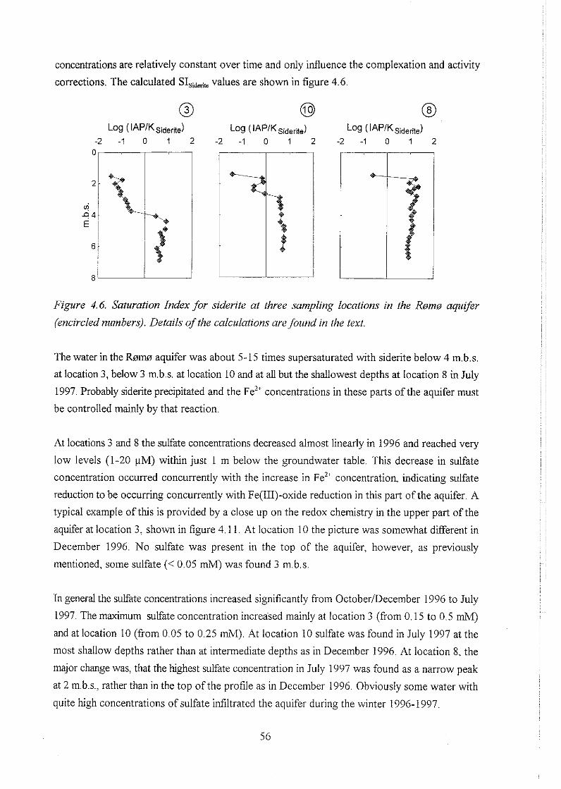
concentrations are relatively constant over time and only influence the complexation and activity
corrections. The calculated SI,,,, values are shown in figure 4.6.
Figure 4.6. Saturation Index for siderite at three sampling locations in the Rsme aquifer
(encircled numbers). Details of the calculations arefotmnd in the text.
The water in the Rnm aquifer was about 5-15 times supersaturated with siderite below 4 m.b.s.
at location 3, below 3 m.b.s. at location 10 and at all but the shallowest depths at location 8 in July
1997. Probably siderite precipitated and the Fez' concentrations in these parts of the aquifer must
be controlled mainly by that reaction.
At locations 3 and 8 the sulfate concentrations decreased almost linearly in 1996 and reached very
low levels (1-20 pM) within just 1 m below the groundwater table. This decrease in sulfate
concentration occurred concurrently with the increase in Fez' concentration, indicating sulfate
reduction to be occurring concurrently with Fe(II1)-oxide reduction in this part of the aquifer. A
typical example of this is provided by a close up on the redox chemistry in the upper part of the
aquifer at location 3, shown in figure 4.11. At location 10 the picture was somewhat different in
December 1996. No sulfate was present in the top of the aquifer, however, as previously
mentioned, some sulfate (< 0.05 mM) was found 3 m.b.s.
In general the sulfate concentrations increased significantly from OctoberiDecember 1996 to July
1997. The maximum sulfate concentration increased mainly at location 3 (from 0.15 to 0.5 rnM)
and at location 10 (from 0.05 to 0.25 mM). At location 10 sulfate was found in July 1997 at the
most shallow depths rather than at intermediate depths as in December 1996. At location 8, the
major change was, that the highest sulfate concentration in July 1997 was found as a narrow peak
at 2 m.b.s., rather than in the top of the profile as in December 1996. Obviously some water with
quite high concentrations of sulfate infiltrated the aquifer during the winter 1996-1997.
When sulfate concentrations were measured in water centrifuged out of the sediment collected for
sulfate reduction rate measurements, even higher concentrations of sulfate (and chloride) were
found at location 10. This is somewhat puzzling, since the sediment was collected less than '/2 m
from where the water samples were taken and only 1-2 weeks later. The measured concentrations
of sulfate and chloride in normal water samples and water centrifuged out of sediment are shown
in figure 4.7.
It was investigated whether one or both sets of measurements were influenced by systematic
errors, but none were detected, and a repeated measurement of the normal water samples gave
similar results (no sediment was left to enable a repetition of that analysis). Moreover, the
diierences between the sulfate and chloride concentrations at the other locations, measured by the
same methods, were minor. Therefore the sulfate and chloride concentrations must actually have
been si@cantly higher in the core taken for sulfate reduction rate measurements at location 10
than in the water samples. This must then reflect a vely sharp front of infiltrating water with a high
ionic strength somewhere upstream from location 10 during the winter 199611997, which
coincidentally was captured by these measurements. The source of the high ionic strength water
could for instance be a high tree catching large amounts of dry deposition during the summer.
The molar relation between sulfate and chloride at location 10 and 8 are up to 0.06-0.13 in the
upper part of the aquifer. These values are higher than the ratio found in seawater (0.045) but are
similar to those previously measured in the RQm0 aquifer (Jakobsen, 1995; Larsen, 1998). The
reason for the high SO:-/CI- relation is most likely an increased concentration of sulfate in
rainwater, due to the oxidation of sulfur compounds from natural and/or anthropogenic sources
in the atmosphere (Savoie & Prospero, 1989; Bates et al. 1992). At location 3 the molar ratio
between SO:- and C1- was up to 0.33 in the upper part of the aquifer in July 1997. Moreover,
while the concentration of sulfate increased significantly here from October 1996 to July 1997, the
concentration of chloride remained practically constant (figure 4.7). For this reason it is not likely,
that the high sulfate concentration at location 3 in July 1997 was derived primarily from rainwater.
A possible explanation is, that a major lowering of the groundwater table, occurring in the summer
of 1996, caused pyrite oxidation to occur in the newly formed unsaturated zone. 1996 was one
of the driest years ever recorded in Denmark, with an exceptional low infiltration. As will be
shown in section 4.4.1, sulfate reduction occurs very close to the groundwater table at the sampled
locations. Pyrite, formed by sulfate reduction during the winter, could therefore be oxidized, when
the groundwater table is lowered during the summer. This is possibly the process responsible for
the large sulfate enrichment in the water at location 3 in July 1997, as well as for some of the
general sulfate enrichment. Fe2' concentrations did not increase in the upper parts of the aquifer
at location 3 from October 1996 to July 1997. Therefore. if pyrite oxidation is responsible for the
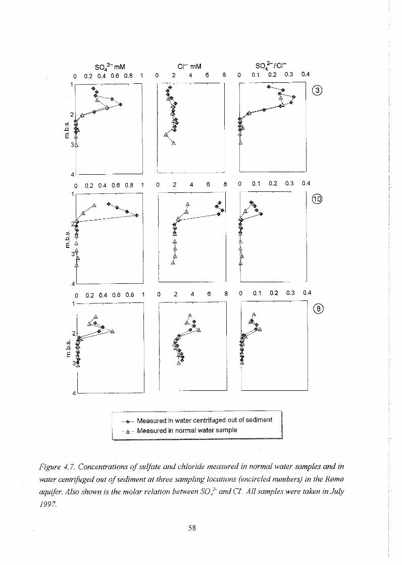
+ Measured in water centrifuged out of sediment
-& Measured in normal water sample
Figure 4 7. Concentrations of suyate and chloride measzrred in normal water samples and in
water centrifuged out of sediment at three sampling locations (encircled numbers) in the Rsmw
aquifer. Also shown is the molar relation between SO,'. and CT. All samples were taken in July
1997.
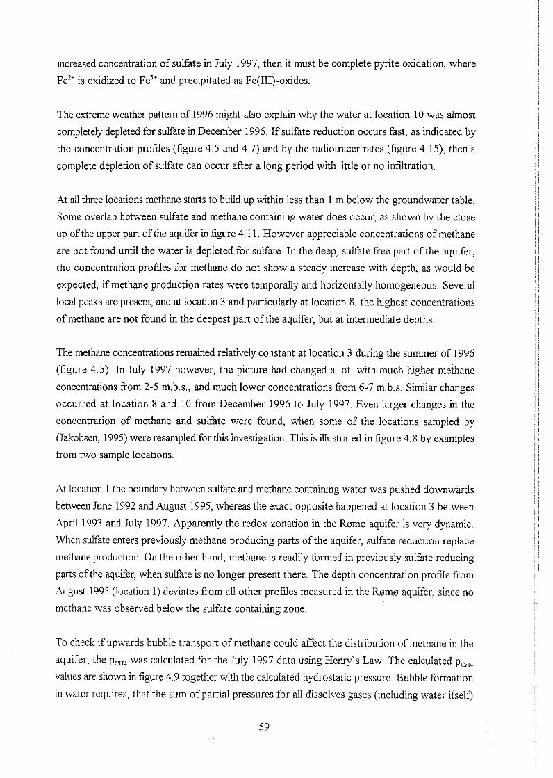
increased concentration of sulfate in July 1997, then it must be complete pyrite oxidation, where
Fez+ is oxidized to Fe3+ and precipitated as Fe(II1)-oxides.
The extreme weather pattern of 1996 might also explain why the water at location 10 was almost
completely depleted for sulfate in December 1996. If sulfate reduction occurs fast, as indicated by
the concentration profiles (figure 4.5 and 4.7) and by the radiotracer rates (figure 4. IS), then a
complete depletion of sulfate can occur after a long period with little or no infiltration.
At all three locations methane starts to build up within less than 1 m below the groundwater table.
Some overlap between sulfate and methane containing water does occur, as shown by the close
up ofthe upper part of the aquifer in figure 4.11. However appreciable concentrations of methane
are not found until the water is depleted for sulfate. In the deep, sulfate free part of the aquifer,
the concentration profiles for methane do not show a steady increase with depth, as would be
expected, if methane production rates were temporally and horizontally homogeneous. Several
local peaks are present, and at location 3 and particularly at location 8, the highest concentrations
of methane are not found in the deepest part of the aquifer, but at intermediate depths.
The methane concentrations remained relatively constant at location 3 during the summer of 1996
(figure 4.5). In July 1997 however, the picture had changed a lot, with much higher methane
concentrations from 2-5 m.b.s., and much lower concentrations from 6-7 m.b.s. Similar changes
occurred at location 8 and 10 from December 1996 to July 1997. Even larger changes in the
concentration of methane and sulfate were found, when some of the locations sampled by
(Jakobsen, 1995) were resampled for this investigation. This is illustrated in figure 4.8 by examples
from two sample locations.
At location 1 the boundary between sulfate and methane containing water was pushed downwards
between June 1992 and August 1995, whereas the exact opposite happened at location 3 between
April 1993 and July 1997. Apparently the redox zonation in the RQms aquifer is very dynamic.
When sulfate enters previously methane producing parts of the aquifer, sulfate reduction replace
methane production. On the other hand, methane is readily formed in previously sulfate reducing
parts of the aquifer, when sulfate is no longer present there. The depth concentration profile from
August 1995 (location 1) deviates from all other profiles measured in the RQms aquifer, since no
methane was observed below the sulfate containing zone
To check if upwards bubble transport of methane could affect the distribution of methane in the
aquifer, the p,,, was calculated for the July 1997 data using Henry's Law. The calculated p,,,
values are shown in figure 4.9 together with the calculated hydrostatic pressure. Bubble formation
in water requires, that the sum of partial pressures for all dissolves gases (including water itself)
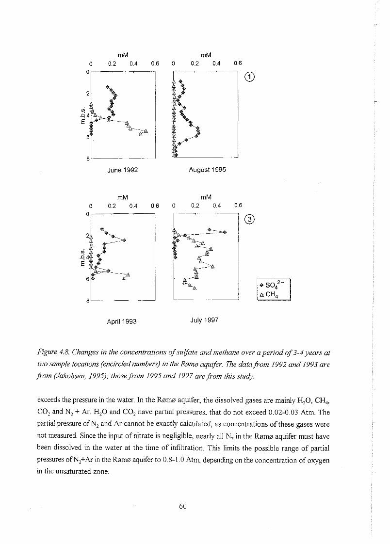
June 1992 August 1995
April 1993 July 1997
Figure 4.8. Changes in the concentvations of sulfclte and methane over a period of 3-4 years at
two sample locations (encirclednumbers, in the Rgmo aquifer. T3e h f a j o r n 1992 and 1993 are
porn (Jakobsen, 1995), those j o m 1995 and I997 nvefr.om this study,
exceeds the pressure in the water. In the b m m aquifer, the dissolved gases are mainly H,O, CH,,
CO, and N, + Ar. H 2 0 and CO, have partial pressures, that do not exceed 0.02-0.03 Atm. The
partial pressure ofN, and Ar cannot be exactly calculated, as concentrations of these gases were
not measured. Since the input of nitrate is negligible, nearly all N, in the R0m0 aquifer must have
been dissolved in the water at the time of infiltration. This limits the possible range of partial
pressures ofN,+Ar in the Rum# aquifer to 0.8-1.0 Atm, depending on the concentration of oxygen
in the unsaturated zone.
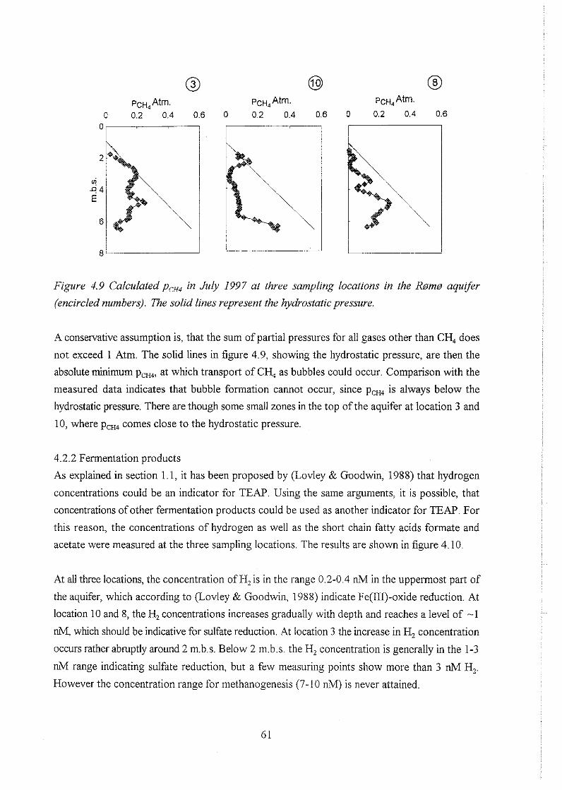
Figure 4.9 Calculated p, in July I997 at three sampling locations in the Rsms aquger
(encircled numbers). The solid lines represent the hydrostatic pressure.
A conservative assumption is, that the sum of partial pressures for all gases other than CH4 does
not exceed 1 Atm. The solid lines in figure 4.9, showing the hydrostatic pressure, are then the
absolute minimum p,,, at which transport of CH, as bubbles could occur. Comparison with the
measured data indicates that bubble formation cannot occur, since p,, is always below the
hydrostatic pressure. There are though some small zones in the top of the aquifer at location 3 and
10, where p,, comes close to the hydrostatic pressure.
4.2.2 Fermentation products
As explained in section 1.1, it has been proposed by (Lovley & Goodwin, 1988) that hydrogen
concentrations could be an indicator for TEAF. Using the same arguments, it is possible, that
concentrations of other fermentation products could be used as another indicator for TEAP. For
this reason, the concentrations of hydrogen as well as the short chain fatty acids formate and
acetate were measured at the three sampling locations. The results are shown in figure 4.10.
At all three locations, the concentration of H,is in the range 0.2-0.4 nM in the uppermost part of
the aquifer, which according to (Lovley & Goodwin. 1988) indicate Fe(II1)-oxide reduction. At
location 10 and 8, the Hz concentrations increases gradually with depth and reaches a level of -1
nM, which should be indicative for sulfate reduction. At location 3 the increase in H, concentration
occurs rather abruptly around 2 m.b.s. Below 2 m.b.s. the H, concentration is generally in the 1-3
nM range indicating sulfate reduction, hut a few measuring points show more than 3 nM Hz.
However the concentration range for methanogenesis (7- 10 nM) is never attained.
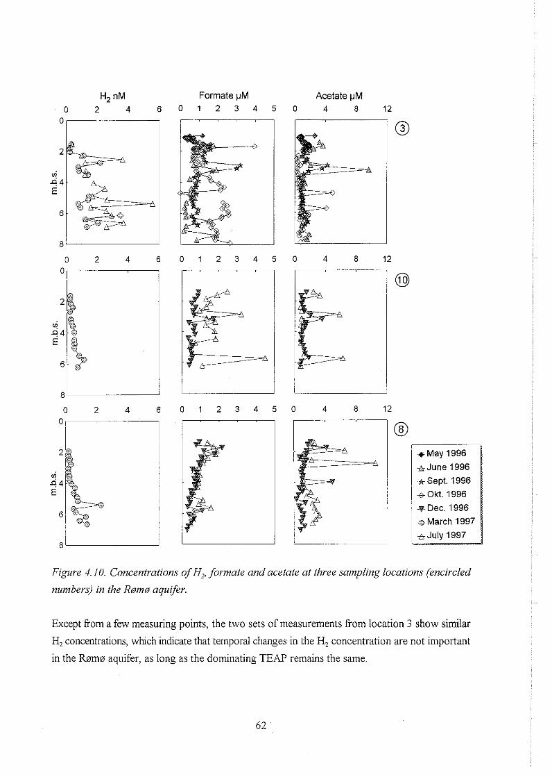
Formate pM
0 1 2 3 4 5 Acetate pM
0 4 8 12
Figure 4.10. Concentrntions of H,, formate and acetate at three sampling locations (encircled
numbers) in the R o m ~ aquqer.
Except from a few measuring points, the two sets of measurements from location 3 show similar
H, concentrations, which indicate that temporal changes in the H, concentration are not important
in the b m s aquifer, as long as the dominating TEAP remains the same.
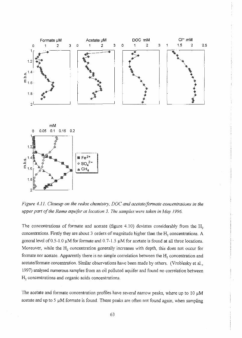
Formate pM Acetate pM DOC rnM CI- mM 0 1 2 3 0 1 2 3 0 1 2 3 1 1.5 2 2.5
Figure 4.1I. Closeup on the redox chemistry, DOC and acetate/frmate concentrntions in the
upperpart of the Romo aquifer at location 3. The samples were taken in May 1996.
The concentrations of formate and acetate (figure 4.10) deviates considerably from the H,
concentrations. Firstly they are about 3 orders of magnitude higher than the H, concentrations. A
general level of 0.5-1.0 pM for formate and 0.7-1.5 pM for acetate is found at all three locations.
Moreover, while the H, concentration generally increases with depth, this does not occur for
formate nor acetate. Apparently there is no simple correlation between the H, concentration and
acetateiformate concentration. Similar observations have been made by others. (Vroblesky et al.,
1997) andysed numerous samples from an oil polluted aquifer and found no correlation between
H, concentrations and organic acids concentrations.
The acetate and formate concentration profiles have several narrow peaks, where up to 10 pM
acetate and up to 5 pM formate is found. These peaks are often not found again, when sampling

is repeated. Possibly they represent temporary nonequilibrium or very local conditions. But many
of these peaks are indicated by one measuring point only, and it can therefore not be ruled out,
that some of them could be outliers resulting from individual pollution of samples.
The general level of formate and acetate concentrations seems to be more constant over time, but
some variations are nonetheless found.
Sometimes a change in concentration is observed for both organic acids, but just as often this is
not the case. There is therefore no simple correlation between the concentration of formate and
acetate either.
Some or all of the changes in the formate and acetate concentrations between the different
sampling times might be due to small scale horizontal variations in the sediment. As explained in
section 2, repeated sampling was done at a distance of 0.5-1.0 m from the original sampling
locations. Given a horizontal flow velocity of 10 mlyr., advective transpofl of organic acids over
such distances would take about 450-900 hours. Since the turnover time for acetate in the RQms
aquifer varies &om 5-500 hours (figure 5.4), this means, that substantial differences in the acetate
concentrations could theoretically exist between sampling points located just 0.5-1.0 m apart.
4.2.3 Ammonium
Ammonium is formed as a byproduct in the decomposition of organic matter. Concentrations of
ammonium at the three sampling locations are shown in figure 4.12.
Figure 4.12. Concenhations of NH,' at three sampling locations (mcircled numbers) in the
Rsms aqztifer. R e samples were taken in December 1996 (location I 0 and8) and in July 1997
(location 3).

The concentration of NH,' increases with depth at location 10 and 8, as would be expected if
decomposition of organic matter by redox processes occurred. This is not the case at location 3,
where the NH,' concentration is nearly constant around 0.02 mM. The highest NH,' concentra-
tions are found at the base of location 8, where a level of 0.08 mM is reached. If a constant
content of N in the decomposed organic matter can be assumed, then it should be possible to
correlate directly the NH,' concentration to the amount of organic matter being decomposed. In
an attempt to do this, the measured NH,' concentrations were plotted against the concentration
of CH, but this gave a very low correlation coefficient (R2 = 0.002). Possible explanations for this
could be, that there are large diierences in the amounts of sulfate or Fe(II1)-oxides that are being
reduced along the diierent flow paths, that the N content in the organic matter being decomposed
varies a lot or that the NH,' concentrations were influenced by ion exchange. Or a combination
of all these factors. Anyhow it seems difficult to obtain usehl information from NH,- concentra-
tions in the Rmn~ aquifer.
4.3 Organic matter in sediment and water
To estimate the size of the different pools of organic matter, the content of DOC @issolved
Organic Carbon) was measured at all three sampling locations. The content of SOC (Sedimentary
bound Organic Carbon) was measured at location 3 only. The measured DOC values are shown
in figure 4.13 The distribution of SOC at location 3, split up in two fractions, is shown in figure
4.14.
DOC mM 0
DOC mM @
DOC mM @
0 1 2 3 0 1 2 3 0 1 2 3
0
2
V1
n 4 E
6
8
Figure 4.13. DOC in the Ram@ nqii$er. Encircled nz~mbers rcjer to .sampling locations.
65
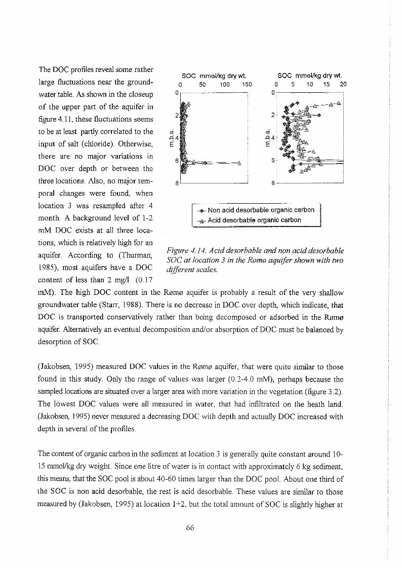
The DOC profiles reveal some rather SOC rnrnollkg dry wt. SOC rnrnollkg dry wt.
large fluctuations near the ground- o 50 100 150 o 5 10 15 20
water table. As shown in the closeup 07, 0 ,
of the upper part of the aquifer in
figure 4.11, these fluctuations seems 2
to be at least partly correlated to the ~ n 4
input of salt (chloride). Otherwise, E
there are no major variations in 6
DOC over depth or between the I I three locations. Also, no major tern- 8 8
poral changes were found, when
location 3 was resampled after 4 1 + Non acid desorbable organic carbon H month. A background level of 1-2 +Acid desorbable oraanic carbon 1 - - I mM DOC exists at all three loca-
tions. which is relativelv high for an - Figure 4.14. Acid desorbable and non acid desorbable
aquifer. According to (Thurman, SOC at location 3 in the Rsmo aquifer shown with two
1985), most aquifers have a DOC different scales, ". content of less than 2 mgll (0.17
mM). The high DOC content in the Ram0 aquifer is probably a result of the very shallow
groundwater table (Starr, 1988). There is no decrease in DOC over depth, which indicate, that
DOC is transported conservatively rather than being decomposed or adsorbed in the %ma
aquifer. Alternatively an eventual decomposition andlor absorption of DOC must be balanced by
desorption of SOC.
(Jakobsen, 1995) measured DOC values in the Rams aquifer, that were quite similar to those
found in this study. Only the range of values was larger (0.2-4.0 mM), perhaps because the
sampled locations are situated over a larger area with more variation in the vegetation (figure 3.2).
The lowest DOC values were all measured in water, that had infiltrated on the heath land.
(Jakobsen, 1995) never measured a decreasing DOC with depth and actually DOC increased with
depth in several of the profiles.
The content of organic carbon in the sediment at location 3 is generally quite constant around 10-
15 mmolkg dry weight. Since one litre of water is in contact with approximately 6 kg sediment,
this means, that the SOC pool is about 40-60 times larger than the DOC pool. About one third of
the SOC is non acid desorbable, the rest is acid desorbable. These values are similar to those
measured by (Jakobsen, 1995) at location 1+2, but the total amount of SOC is slightly higher at
location 3. The only elevated SOC values at location 3 are found 1.0-1.3 m.b.s. and as a large but
narrow peak 6.2 m.b.s. The sediment from 1.0-1.3 m.b.s. is submerged in the saturated zone for
most of the time, but in dry years like 1996 the groundwater table is lowered to slightly below this
depth. A large amount of root fragments was observed at this depth, which could contribute to
the elevated SOC content.
The large but narrow peak in SOC 6.2 m.b.s. probably reflects a different sedimentary
environment. In most of the sediment cores sampled at location 3, the sediment had a very
dzerent visual appearance around 6.2 m.b.s. being much darker and more fine grained than other
sediment from the h m aquifer. When base was added to such sediment, the water turned nearly
black, probably due to extraction of organic matter from the sediment. As shown in figure 4.4,
there was also a very high content of SIC (both whole shells and shell fragments) in this sediment.
The fine grain size and the correlation between the content of SOC and SIC in this sediment
strongly indicates a marine origin.
The layer with a high SOC content around 6.2 m.b.s. was not observed in all cores from location
3 and may not have any large horizontal extension. Similarly looking thin (a few cm) layers of
dark, fine grained, shell rich material, turning black by addition of base, were sometimes found also
at other depths (always below 5 m.b.s.) at location 3 and in sediment from the deepest part at
location 10.
To obtain qualitative information about the organic matter in the h m n aquifer, H A S (humic
acids) and F K s (hlvic acids) were isolated from water and sediment at four depths at location 3
The samples were taken in May-September 1996 and the isolations were canied out by the Plant
Biology and Biogeochemistry Dep&ment, RIS0 National Laboratory. The isotopic composition
ofthe isolated F K s and W s were determined by the AMS Laboratory, Institute of Physics and
Astronomy, University of Aarhus. The results are shown in table 4.1
The dissolved F K s and HA's are modern at all depths and have 6°C values in the -24 "I,, to -28
"I,,, range, that is normally associated with terrestrial Calvin cycle plants (Spalding et al 1978)
Their origin must be the present soil zone, and old organic carbon, deposited with the sediment,
contributes very little to dissolved FA'S and W s . This is different from other Danish aquifers,
where similar characterizations of FA'S and W s have been carried out. In the Skagen and Fjand
aquifers, the dissolved F K s and H K s originate from the sediment, and in the Tuse Nses aquifer,
they originate partly from the sediment and partly from the soil zone (Grnn et al 1996).
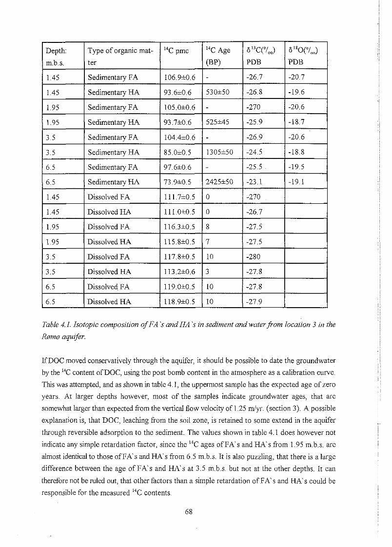
Table 4. I. Isotopic composition of FA k and HA 's in sediment and waterj?om location 3 in the
R0m0 aquifer.
6.5
EDOC moved conservatively through the aquifer, it should be possible to date the groundwater
by the 14C content ofDOC, using the post bomb content in the atmosphere as a calibration curve.
This was attempted, and as shown in table 4.1, the uppermost sample has the expected age of zero
years. At larger depths however, most of the samples indicate groundwater ages, that are
somewhat larger than expected from the vertical flow velocity of 1.25 d y r . (section 3). A possible
explanation is, that DOC, leaching from the soil zone, is retained to some extend in the aquifer
through reversible adsorption to the sediment. The values shown in table 4.1 does however not
indicate any simple retardation factor, since the 14C ages of F A s and HA's from 1.95 m.b.s. are
almost identical to those ofFA's and HA's from 6.5 m.b.s. It is also puzzling, that there is a large
difference between the age of F A s and HA'S at 3.5 m.b.s. but not at the other depths. It can
therefore not be ruled out, that other factors than a simple retardation of F A s and H A S could be
responsible for the measured '" contents.
Dissolved HA 10 118.910.5 -27.9

The "C ages determined for sedimentary H A S are very similar to the expected age of the
sediment: around 500 years in the top of the aquifer, increasing to 2400 years 6.5 m.b.s. This
indicates, that the sedimentary HA's are remnants of the organic matter, that was deposited with
the sediment. The F A s in the sediment have calculated 14C ages, that are considerably younger
than the HA's. The "C content in all four samples are however significantly below the values, that
existed in the atmosphere in 1996 (about 11 1 pmc), and it decreases with depth. This indicates,
that the FA's in the sediment are a mixture of modem organic carbon fiom the soil zone and older
organic carbon. The sediment has been exposed to organic matter, leaching from the soil zone, for
several houndred years. Therefore, the young age of the F A s adsorbed to the sediment show, that
the part of them, that is derived from the soil zone must be turned over by desorption or
decomposition within a few years.
The 613C values found inFA's from the sediment are quite constant over depht and all values are
in the -24 %, to -28 %, range, indicating a terrestrial origin (Spalding et al. 1978). Only in the
sample kom 6.5 m.b.s. is a somewhat lower 613C value found, which might indicate some content
of marine F A s in this sample. In contrast the 613C values for sedimentary HA's increase
consistently with depth. In the sample fiom 6.5 m.b.s. the 613C value even fall in the -22 "I,, to -24
"/,, range, that is typical for marine organic matter (Nissenbaum & Kaplan, 1972). This further
supports, that the sediment from the lower part of the aquifer was deposited in a marine
environment. The 613C value found in sedimentary HA's fiom 3.5 m.b.s. is also pretty close to the
marine range. Perhaps this sediment was deposited at the upper edge of the wide marine foreland,
that still exists on the b m Island, or slightly behind it in an area, that was occasionally flushed
by the sea. In such a sedimentary environment, it is perfectly logical, that the organic matter
deposited is partly of marine and partly of terrestrial origin.
4.4 Rates of redox processes
While the concepts, that were described in the previous section, might give useful information
about the occurrence of redox processes, much more reliable and detailed information can be
obtained by measuring the rates of the redox processes directly, using radiotracers (section 1.4).
Sulfate reduction rates, methane production rates, acetate turnover rates and methane oxidation
rates were therefore measured by the methods described in section 2.5.
4.4.1 Sulfate reduction rates
The measured sulfate reduction rates are shown in figure 4.15 together with the concentrations
of SO:. and C1-, that were measured in water from the cores used for the rate measurements.
Sulfate reduction takes place in the upper, sulfate containing part of the Ram0 aquifer at all three
locations. The highest sulfate reduction rates varies from 1.3 mMiyr. at location 8 to 2.8 mM/yr.
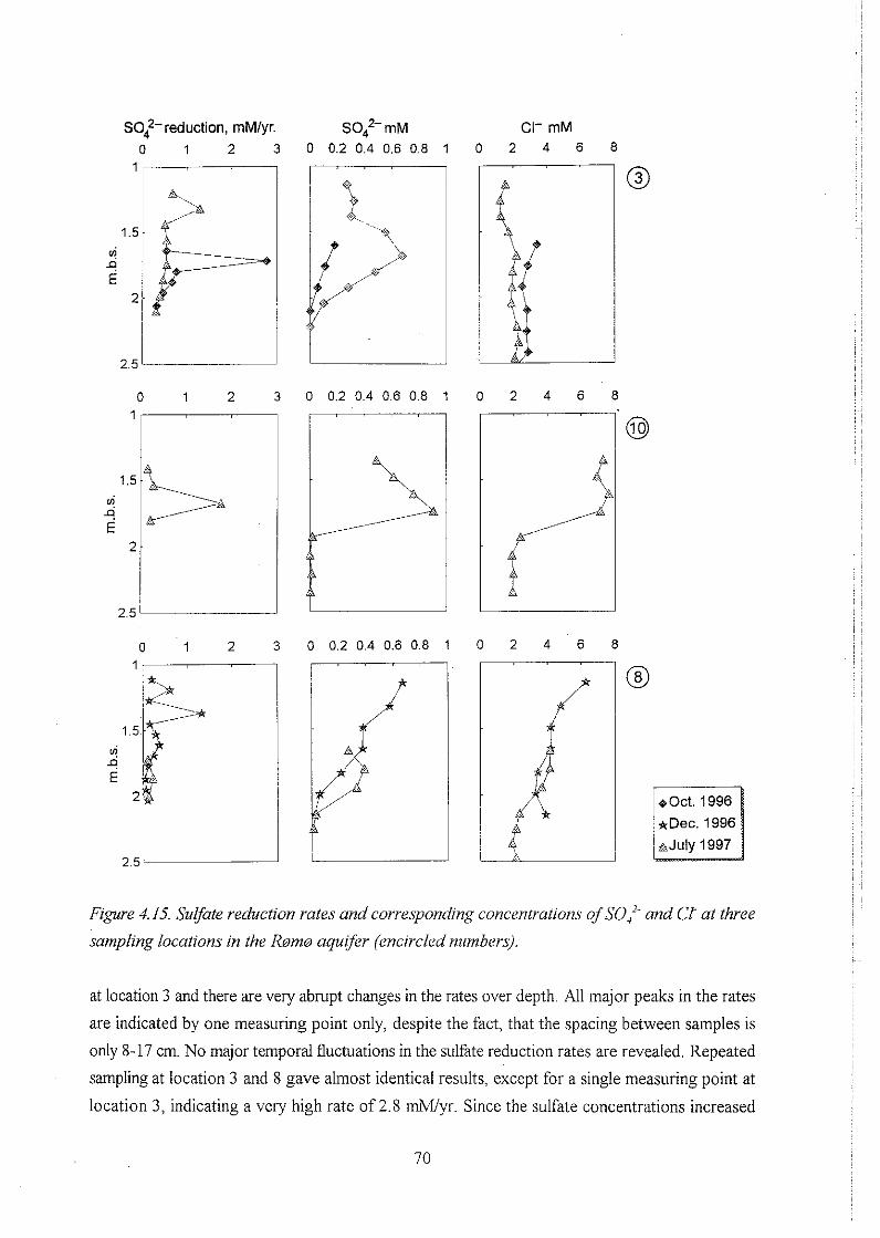
~0~~- reduc t ion , rnM1yr. 50:- rnM CI- rnM 0 1 2 3 0 0.2 0.4 0.6 0.8 1 0 2 4 6 8
Figure 4.15. Sulfate reduction rates and corresponding concentrations of SO:- and Ct at three
sampling locations in the Rsmw aqufer (enc~rcled nzimber~j.
at location 3 and there are very abrupt changes in the rates over depth. All major peaks in the rates
are indicated by one measuring point only, despite the fact, that the spacing between samples is
only 8-17 cm. No major temporal fluctuations in the sulfate reduction rates are revealed. Repeated
sampling at location 3 and 8 gave almost identical results, except for a single measuring point at
location 3, indicating a very high rate of 2.8 M y r . Since the sulfate concentrations increased

significantly from OctoberKlecember 1996 to July 1997, this indicates, that the sulfate
concentration does not have any large iduence on the sulfate reduction rates in the RQms aquifer.
Other factors, like the reactivity of organic matter, must be rate h t i n g . This is in accordance with
the findings from other low-sulfate freshwater sediments, where the half-saturating sulfate
concentration has been determined to something like 0.05-0.10 mM p o d e n & Tuttle, 1993).
Since the sulfate concentration is well above this level in most parts of the sulfate reducing zone,
it is reasonable, that the sulfate reduction rates are largely independent on the sulfate concentra-
tion.
A comparison between the measured sulfate reduction rates and the rates, that can be calculated
from the concentration depth profiles of sulfate, reveals no major discrepancy. A similar finding
was made by (Jakobsen, 1995). Accordingly, the rate measurements seems to be reliable.
However, while the general level of rates agrees well with the concentration profiles, much more
details are disclosed by the directly measured rates. The rates measured in July 1997 are generally
much lower than those, that could have been calculated from the concentration profiles by - erroneously - assuming a constant input of sulfate over time (figure 4.5 and 4.7). The rates are not
constant over horizontal distances of more than a few metres either. At location 8 the rates
measured 1.5-2.0 m.b.s. in both December 1996 and July 1997 are much too low to explain the
decrease in sulfate concentration with depth. In agreement with this, sulfate was found at larger
depth downstream from location 8 in December 1996 (data not shown). In conclusion, much more
detailed and reliable information about sulfate reduction rates are obtained by measuring the rates
directly, using a radiotracer.
4.4.2. Methane production rates
The measured methane production rates are shown in figure 4.16 together with the measured
methane concentrations. Also shown in figure 4.16 is the calculated % of the total measured
methane production, that occurred with acetate as the precursor. This was calculated by
interpolation of the CO, reduction rates to the depths, where acetate fermentation rates had been
measured.
At all three locations, methane production does not take place at appreciable rates, before sulfate
is depleted from the water. This indicates, that sulfate reducing bacteria can outcompete
methanogens for H, and acetate in the RQms aquifer. At location 3 appreciable methane
production begins right below the depth (2 m.b.s.), where sulfate is depleted from the water. At
location 10 and 8 however, appreciable methane production does not begin until 1-3 m below the
depth, where sulfate is depleted from the water. This indicates, that methanogens are being
outcompeted for H, and acetate by a redox process other than sulfate reduction in the intervals
2-3 m.b.s. at location 10 and 2-4 m.b.s. at location 8. However, even when other electron
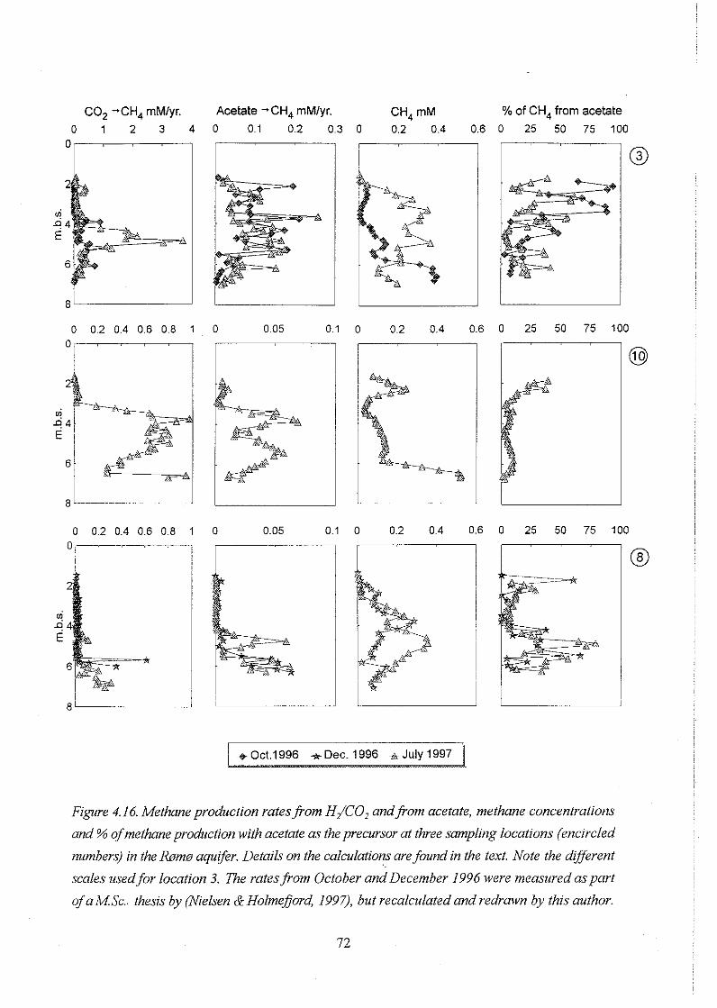
Acetate -CH4 mMlyr. 0 0 1 0.2 0.3
CH, mM % of CH, from acetate
0 0.2 0.4 0.6 0 25 50 75 100
Figure 4.16. Methane production ratesfrom HJCO, andfiom acetate, methane concentrations
and % of methane prodziction with acetate as the precursor at three sampling locations (encircled
mrmhers) in the &m@ aquifeu. Details on the calculations are fmnd in the text. Note the dzfferent
scales zrsed for location 3. The ratesfiom October and December 1996 were measzlred aspart
of a MSc. thesis by (iVielsen &Holmejord, 1997), but recalculated and redruwn by this author.

accepting processes dominate, low rates of methane production could always be measured.
Methane production is therefore never completely excluded by other redox processes.
The total rate of methane production varies highly over depth and between the sampled locations.
The maximum rates vary from 0.6 d y r at location 8 to 4 d y r at location 3. Overall, there
is a large degree of covariation between the CO, reduction rates and the acetate fermentation
rates. In particular, a high CO, reduction rate is never measured concurrently with a very low
acetate fermentation rate or vice versa. Any competitive suppression of methane production must
therefore occur concurrently for the CO, reduction and the acetate fermentation pathways.
In general, CO, reduction is the most important pathway of methane production in the Rams
aquifer. This is in accordance with the estimates in previous studies, that were based on the
isotopic composition of methane (Coleman et al. 1988; Grossman et al. 1989; Aravena et al. 1995;
Zhang et al. 1998). The relative importance of CO, reduction and acetate fermentation is far from
constant, and in some parts of the aquifer, acetate fermentation is even the dominating process.
Many of the small scale variations in the % of methane derived from acetate appears to be quite
chaotic, and possibly some of these variations are simply the result of the slightly different
sampling locations (cores were taken '/2 m apart), minor errors in the determination of depths or
perhaps analytical noise. A significant general trend is however, that when methane production
rates are high (4-5 m.b.s. at location 3 and 3-5 m.b.s. at location lo), then only a minor part of the
methane (5-10 %) is produced by acetate fermentation. At lower but still appreciable methane
production rates, acetate is often a much more important substrate for methane, accounting for
20-90 % of the methane production.
The repeated sampling at location 3 and 8 showed almost identical acetate fermentation rates at
most depths. There are some local peaks in the acetate fermentation rates though, that are present
in one of the measurements but not in the other. Most noticeable is the peak around 5 m.b.s. at
location 8 in July 1997. These local peaks could reflect temporal but also horizontal differences
in the rates, since the cores were taken about 55 m apart. Still, when the overall picture is
considered, the acetate fermentation rates were essentially the same at the different times of
sampling.
The same cannot be said about the CO, reduction rates. There are some parts of the aquifer, where
the CO, reduction rates were essentially the same at the two times of sampling, but there are large
differences in other parts of the aquifer. Most profound is the very large peak in the CO, reduction
rate at location 3, 4-5 m.b.s., that was found in July 1997 but not in October 1996. Also at shallow
depths (2-4 m.b.s.) was the CO, reduction rate at location 3 much higher in July 1997 than in
October 1996.
The methane production rates measured with the radiotracers deviate a lot from those, that can
be calculated from the concentration depth profiles of methane. In the upper part of the aquifer,
the measured rates are generally much lower than the calculated, and in the deeper part of the
aquifer, they are often much higher (location 3 and 10). The concentration depth profiles even
indicate negative rates (decreasing concentration with depth) in parts of the aquifer, where
methane production takes place at high rates. This could theoretically be an effect of methane
oxidation, but as will be shown in the following section, this is not the case. Accordingly, the
methane production rates must be highly variable, temporally andlor horizontally, in the Rmms
aquifer, and a direct measurement of the rates is necessary to get a reliable picture of where in the
aquifer, methane production occurs.
4.4.3 Acetate turnover rates
As explained in section 1.4, the 14C-methyl group in 214C-acetate should end up as "CH,, if 2 - 1 4
acetate is fermented by methanogenic bacteria. If, on the other hand, 2-I4C-acetate is oxidized by
other bacteria than methanogens, the 14C-methyl group should end up as 14COz. The measured
rates of acetate oxidation and fermentation are shown in figure 4.17. Also shown in figure 4.17
is the respiration index of acetate, RI, defined by e.g. (Sansone &Martens, 1982) as:
where ['TO, ] and [l4CH,] are the activities of 14C02 and I4CH4 formed from 2-14c-acetate during
the incubation.
Figure 4.18 shows a cumulative plot of the rates of acetate oxidation and fermentation, where a
smaller y-axes scale gives a better overview of the rates in the deeper part of the aquifer.
The rates of acetate oxidation are very high at the most shallow depths in the aquifer, where
sulfate reduction (figure 4.15) and Fe(II1)-oxide reduction (indicated by the Fez' concentration
profiles, figure 4 5) takes place. The acetate oxidation rates measured in the sulfate containing
zones at location 3 and 8 are similar to or even higher than the sulfate reduction rates measured
at the same depths. Some acetate is probably also being oxidized by Fe(II1) reducers at these
depths, but nonetheless this indicates, that acetate is a very important precursor for sulfate
reduction in this part of the aquifer, since one mole of acetate is necessary for the reduction of one
mole of sulfate. At location 10 no measurements of acetate oxidation rates were made in the
sulfate containing zone, so the same comparison cannot be made there.
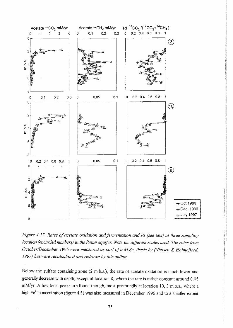
Acetate -C02 rnMlyr. 0 1 2 3 4
0, I
Acetate -CH4 mMlyr. RI I4co2 I( '~CO~+'~CH~) 0 0.1 0.2 0.3 0 0.2 0.4 0.6 0.8 1
Figure 4.17. Rates of acetate oxidation and fermentation and RI (see text) at three sampling
location (encirclednumbers) in the &m@ aquifer. Note the dzflerent scales used. The rates ffom
October/December I996 were measured as part of a MSc. thesis by mielsen & Holmefiord,
1997) but were recalculated and redrawn by this author.
Below the sulfate containing zone (2 m.b.s.), the rate of acetate oxidation is much lower and
generally decrease with depth, except at location 8, where the rate is rather constant around 0.05
mMiyr. A few local peaks are found though, most profoundly at location 10, 3 m.b.s., where a
high Fez+ concentration (figure 4.5) was also measured in December 1996 and to a smaller extent
Rate mM/yr. 0 0.1 0.2 0.3 0.4 0.5
Rate mMlyr. 0 0 1 0.2 0.3 0.4 0.5
Rate mM/yr. 0 0.1 0.2 0.3 0.4 0.5
8 ' I
July 1997
Rate mMlyr. 0 0 1 0.2 0.3 0.4 0.5
8 I
Oct. 1996
8 ' 1
July 1997 July 1997
Rate rnMlyr, 0 0.1 0.2 0.3 0.4 0.5
Dec. 1996
Figure 4.18. Cumulative plots of acetate oxidation (inner) and fermentation (outer) rates at three
sumpling locations (encircled numbers) in the Romo aquifer. The rates from October/December
1996 were measured as part of a MSc. thesis by mielsen & Holmejord, 1997) but were
recalculated and redrawn by this author.
in July 1997, when the rate measurement was made. In the deeper parts of the aquifer (4-7 m.b.s.),
the highest acetate oxidation rates are again found at location 3 (0.05-0.30 M y r . ) and the lowest
at location 10 (0.02-0.06 mM/yr.). In general, the acetate oxidation rate did not change much from
OctoberDecember 1996 to July 1997. The only exception from this is the most shallow depths
at location 8, where values up to 0.9 My . were found in July 1997 rather than the 0.35 mM/yr.
found in December 1996.
As would be expected from the low methane production rates, only a minor fraction of the 2-'kc-
acetate ended up as I4CH4 in samples from the sulfate containing zone. The suppression of
methane production from acetate is strongest in the uppermost sample at location 8, where only
0.04 % of the acetate is turned over by methanogens. But even at depths down to 4 m.b.s., not
more than -1 % of the acetate is consumed directly by methanogens. At the other locations, the
suppression of methane production from acetate in the upper part of the aquifer is not quite as
strong, but still evident. At larger depths, methane production from acetate takes place at
sigdcant rates, and accordingly the RI decrease to 0.25-0.85 (figure 4.17). Still, 25 to 85 % of
the acetate is oxidized rather than fermented in these parts of the aquifer.
4.4.4 Methane oxidation rates
As discussed in section 2.5, the measured methane oxidation rates seems to be hampered by
systematic errors and are therefore only maximum estimates. The rates are shown in figure 4.19,
together with the measured concentrations of methane and sulfate, the turnover of the injected
"CH, tracer during the incubations and the relation between methane oxidation and methane
production rates. The latter was calculated by interpolation of the acetate fermentation and CO,
reduction rates to the depths, where the methane oxidation rates were measured.
The methane oxidation rates are considerably lower than the rates of sulfate reduction and
methane production. The highest rates vary from 0.017 rnMiyr at location 3 to 0.07 mM/yr. at
location 8, and these are even maximum estimates. So in general, methane oxidation is not a
quantitatively important process in the Ram aquifer. Unlike the findings from marine sediments
(e.g. Iversen & Blackburn, 1981; Devil, 1983; Iverson & Jerrgensen, 1985, Hoehler et al., 1994),
there is no indication for sulfate being an important electron acceptor for the small amount of
methane, that is being oxidized. The methane oxidation rates are very low in the sulfate containing
part of the aquifer and increase considerably below the depth of sulfate depletion.
The turnover of injected tracer is relatively constant over depth at location 3 and 10 and the
methane oxidation rates are therefore mainly controlled by the methane concentration here. This
might indicate, that the apparent methane oxidation measured here is mainly the result of analytical
artefacts: a tiny bit of 14C02 is always found in the analysis (figure 2.5). At location 8, on the other
hand, the turnover of tracer is generally larger and there seems to be some systematic variations
aver depth, that might indicate, that we are closer to measuring real rates. There is however still
the problem, that the finding of 'TO, is largely independent of the finding of "CH,, even at
location 8 (figure 2.5). This discrepancy remains unexplained. Despite the systematic error
introduced by this artefact, it is evident, that the rate of methane oxidation is largely independent
of the rate of methane production. Where the methane production rates are high (4-5 m b.s at
location 3 and 3-5 m.b.s. at location 10) < 1 % of the produced methane is being reoxidized,
whereas a much larger fraction of the produced methane is being reoxidized in the parts of the
aquifer, where methane has been transported into areas with low methane production rates (2-3
CH,oxidation mMlyr. CH,,SO,~- mM Turnover ofCH4 tracer % CH4 ox. % of CH, prod.
0 0.02 0.04 0.06 0.08 0 0.2 0.4 0.6 0.8 1 0 0.05 0.1 0 4 8 12
Figure 4.19. Mmcimum methane oxidation rates at three sampling locations (encircled nzrmbers)
in the R0m0 aqulfer, concentratjons of methane and slrlfnte, tzrrnover of injected I4CH4 tracer and
relation between methane oxidation and methane prociuction. Details on the calcz~lations ore
found in the text.
m.b.s, at location 10 and 2-4 m.b s. at location 8). At location 8 net methane oxidation even seems
to be taking place, but due to the previously mentioned problems, the evidence for this is highly
uncertain.
4.5 Isotopic composition of methane and TIC
As discussed in section 1.2, the isotopic composition of methane might be used to deduce the
dominant pathway of methane production and to determine whether a significant fraction of the
methane has been reoxidized. The isotopic composition of methane is shown in figure 4.20. The
samples were prepared by the Geological Survey of Denmark and Greenland and analysed by the
Geological Institute, University of Copenhagen.
6l3CCH, varies from -50 "I,, to -80 0/,,, the highest values being found in the upper part of the
aquifer at location 8 and 11. These values are within the range normally found for bacterially
produced methane, that is not sigruficantly intluenced by methane oxidation or by reservoir effects
(Whiticar et al. 1986; Whiticar & Faber, 1986). 6D, is quite constant; values from -320 ol,, to
-300 "I,, are found in the four samples analysed. These values are lower than those previously
measured in deep aquifers (Coleman et al. 1988; Grossman et al. 1989; Aravena et al. 1995; Zhang
et al. 1998). This indicate, that acetate fermentation is more important in the shallow &ma aquifer
than in deep aquifers. In the diagram proposed by (Whiticar et al. 1986, figure 1.3 in this text), the
Ram0 methane would even be classified as an acetate fermentation type.
Usiig the diagram proposed and used by (Aravena et al. 1995) for Canadian aquifers (figure 1.4),
and assuming that &Dm, is -70 "/,,, which is typical for Danish aquifers (Buchardt, 1998), we
would conclude, that 40-50 % of the methane in the R a m aquifer is produced by acetate
fermentation and the remainder by CO, reduction. This is a slightly higher contribution of acetate
fermentation than shown by the rate measurements. It should be remembered though, that the D/H
fractionation factor for the methanogenic bacteria, on which the diagram in figure 1.4 is based,
might be diierent from the D/H fractionation in the &ma aquifer. For this reason, classification
diagrams as those shown in figure 1 3 and 1.4 can only be approximations to a complex reality.
613C, and I T n , values were determined at location 3. The samples were analysed at the AMS
Laboratory, Institute of Physics and Astronomy, University of Aarhus. The results are shown in
table 4.2.
The increase in 6 l3CnC over depth at location 3 is probably caused by calcite dissolution, that
occurs below 4 m.b.s (figure 4.3). The values found above 4 m b.s. indicates an organic origin of
the TIC and the 14C content is very close to the current content in the atmosphere (1 11 pmc). In
contrast, the 613C,c values measured below 4 m.b.s. are between the values, that would be
expected for organic carbon (-25 "I,,) and for dead carbonate (0 yo). Just as would be expected,
if calcite dissolution occurred, releasing one mole of TIC form carbonate for each mole of
organically derived C02. At two depths (4.9 m.b.s. and 6 5 m.b.s.) the 6'3Cnc values indicate a
larger contribution from dead carbonate than from organic matter. This is not likely to be
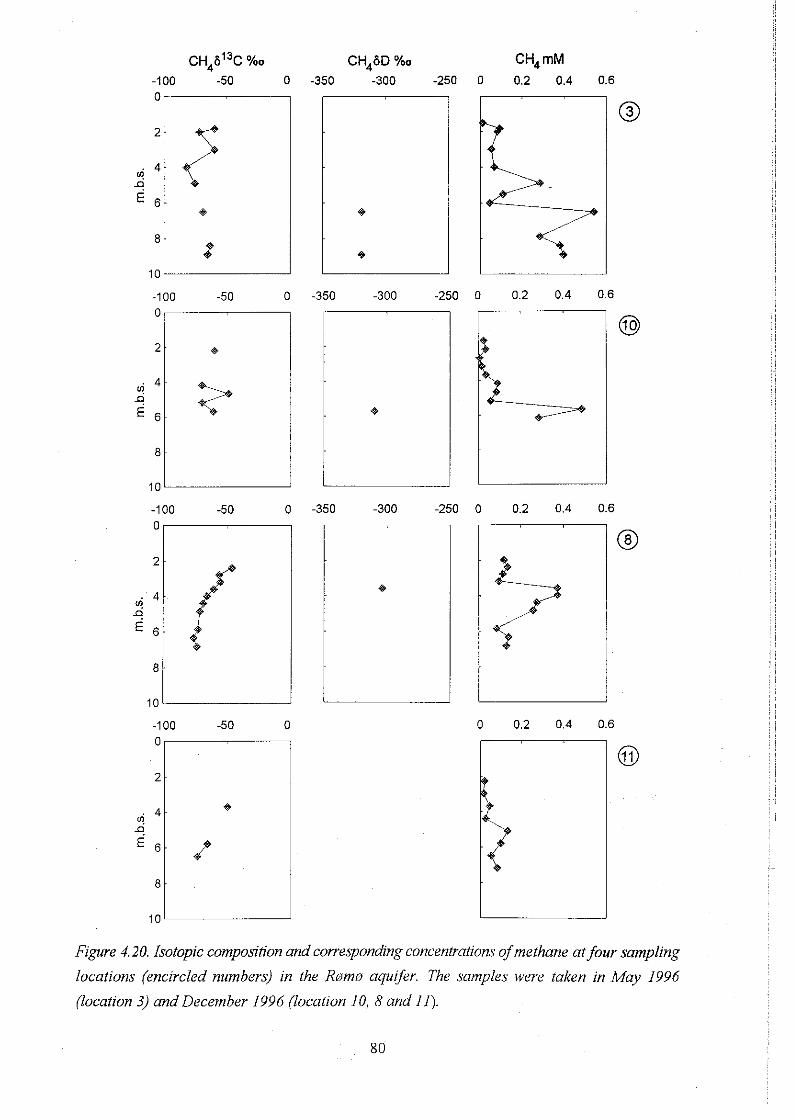
CH,~'~C %o CH46D %o CH, mM -100 -50 0 -350 -300 -250 0 0.2 0.4 0.6
Figure 4.20. Isotopic composition and cove~ponding concentrations of methane at four sampling
locations (encircled numbers) in the Rwmn aquijier. The samples were taken in May 1996
(location 3) and December I996 (location 10, Rand 11).
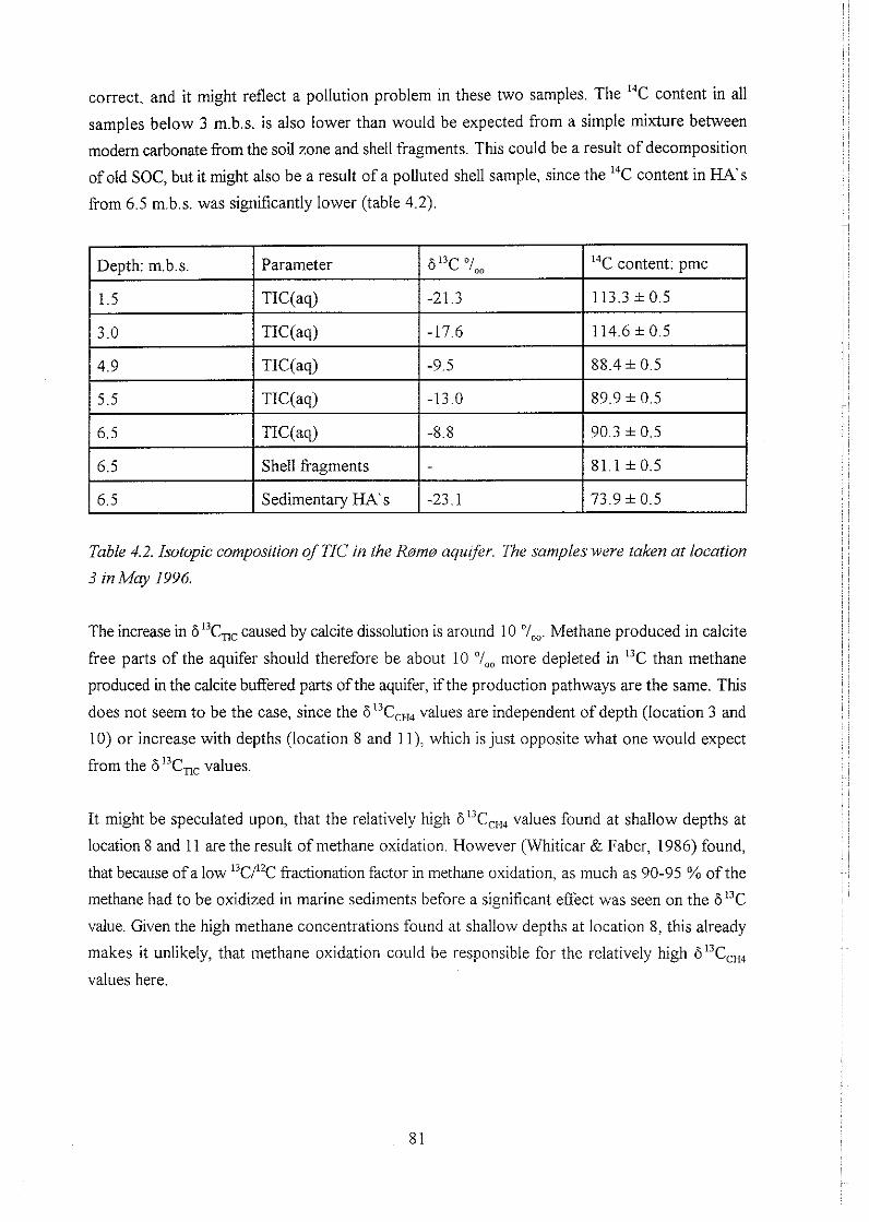
correct, and it might reflect a pollution problem in these two samples. The IJC content in all
samples below 3 m.b.s. is also lower than would be expected from a simple mixture between
modem carbonate fiom the soil zone and shell fragments. This could be a result of decomposition
of old SOC, but it might also be a result of a polluted shell sample, since the 14C content in H A S
from 6.5 m.b.s. was significantly lower (table 4.2).
Table 4.2. Isotopic composition of TIC in the R n m ~ nqzr$er. fie snmples were taken at location
3 in Mq 1996.
The increase in 613C,, caused by calcite dissolution is around 10 "I,,. Methane produced in calcite
free parts of the aquifer should therefore be about 10 "I,, more depleted in 13C than methane
produced in the calcite buffered parts of the aquifer, ifthe production pathways are the same. This
does not seem to be the case, since the 613C,,, values are independent of depth (location 3 and
10) or increase with depths (location 8 and 1 l), which is just opposite what one would expect
from the 6I3C,, values.
It might be speculated upon, that the relatively high 6l3CCH, values found at shallow depths at
location 8 and 11 are the result of methane oxidation. However (Whiticar & Faber, 1986) found,
that because of a low 13C/12C fractionation factor in methane oxidation, as much as 90-95 % of the
methane had to be oxidized in marine sediments before a significant effect was seen on the 613C
value. Gven the high methane concentrations found at shallow depths at location 8, this already
makes it unlikely, that methane oxidation could be responsible for the relatively high 613C,H,
values here.

5. Discussion
5.1 Rates of methane production, sulfate reduction and organic matter decomposition
The rates of sulfate reduction and methane production measured by radiotracers in the b m aquifer in this study and by (Jakobsen & Postma, 1994; Jakobsen, 1995) might be compared to
those measured in marine and lake sediments with the same methods. In table 5.1 is shown some
examples of maximum rates of sulfate reduction and methane production in sediments, measured
by radiotracers. The rates were originally expressed in many different ways, but have been
recalculated to mmol C/(litre sediment*year) to enable a comparison.
Table 5.1. Compnrjson of mc~ximzim mtes of szrlfnte redzictiow and methane production in
sediments. All rates were measured by radiotrncers.
Lake Mendota
A wide span of sulfate reduction and methane production rates exists in sediments and the rates
do not appear to be controlled by the salinity of the sediment. The rates in the RQm0 aquifer are
in the lower end of the range, but are similar to or higher than the rates in some lake sediments
(Lake Washington and Lake Woods). On the other hand they are more than 2 orders of magnitude
lower than the rates in Lake Mendota and Cape Lookout Bight (C.L.B.).
In contrast, the rates in the Ram0 aquifer are orders of magnitudes higher than the rate estimates,
that can be derived by the more indirect methods of using concentration gradients or ground water
ages in deeper aquifer systems (Chapelle & McMahon, 1991; McMahon & Chapelle, 1991;
Aravena et al. 1995). Overall, there is little doubt, that these differences mainly reflects the
Methane production 700 (Phelps & Zeikus, 1985)
availability of reactive organic matter (Eierner, 1985). In aquifer systems the most important
control on the rates is the age and reactivity of the organic matter present (Jakobsen & Postma,
1994). In the young and shallow b m s aquifer, the organic matter is young and reactive, whereas
the organic matter in deep aquifer systems is much older and accordingly has a low reactivity,
since the most reactive part was decomposed long ago (Jakobsen & Postma, 1994). In marine and
lake sediments the rates are influenced mainly by the sedimentation rate of organic matter, since
all organic matter here is young, at least until it is buried deep into the sediments. As an example,
the much studied marine Cape Lookout Bight has a very high rate of organic matter sedimentation
and accordiigly higher rates of sulfate reduction and methane production than many other marine
sediments (Hoehler, 1998).
Cape Lookout Bight is the only one of the sites shown in table 5.1, where the maximum rate of
sulfate reduction is considerably larger (six times) than the maximum rate of methane production.
Most likely this reflects, that sulfate reduction takes place in the upper part of the sediment, where
the most reactive organic matter is present. In lake sediments the penetration of sulfate into the
sediment by d i i s ion and bioturbation is much smaller than in marine sediments, and accordingly
the maximum rate of methane production might actually be higher in lake sediments than the
maximum rate of sulfate reduction (Lake Washington). The values shown in table 5.1 for the
b m 0 aquifer are measured in the same sediment (location 3) at times where sulfate was
presentlabsent (figure 4.8). The very values indicate, that it does not have any major impact
on the rate of organic matter decomposition whether the TEAP is sulfate reduction or methane
production. Perhaps because the energy released by these two processes is not very different, as
shown in figure 1.1. Introduction of an electron acceptor with a much higher energy yield per mole
carbon, like 0, or NO,; might lead to a different result, and it cannot be induced from these data,
that the rate of organic matter decomposition is generally independent of the TEAP.
In marine and lake sediments, a rate maximum is usually found near the surface of the sediment
and below this point the rate decreases with depth, due to a reduced availability of reactive organic
matter (see e.g. some of the studies referred in table 5.1). In an aquifer, a similar distribution of
rates over depth would be expected, if DOM (Dissolved Organic Matter), leaching from the soil
zone, is the main electron donor for the redox processes, since the most reactive part of DOM
would be expected to be decomposed first. The rate of acetate turnover (figure 4.17) decreases
sharply with depth in the Ram aquifer, and it is therefore likely, that DOM, leaching from the soil
zone, is the main source of acetate. In principle, this should result in a decrease in DOC (Dissolved
Organic Carbon) over depth in the upper part of the aquifer, but such a decrease would be very
difficult to detect because of the large and unsystematic fluctuations in DOC near the groundwater
table (figure 4.13).
However, the highest rates of methane production (this study) and sulfate reduction (Jakobsen,
1995) are measured in the deeper part of the aquifer, which speaks against DOM as the only
electron donor. It might be argued of course, that the total rate of organic matter decomposition
could still decrease with depth, ifother redox processes like Fe(II1)-oxide reduction occur at high
rates in the upper part of the aquifer. However, the rates of Fe(II1)-oxide reduction, that can be
calculated from concentration-depth profiles (figure 4.5 and Jakobsen, 1995), result in carbon
oxidation rates, that are considerably lower than those resulting from sulfate reduction and
methane production. Accordingly the carbon oxidation rates are actually higher in the deeper part
of the aquifer at many of the locations, which speaks against DOM as the main electron donor.
Moreover, a significant decrease in DOC with depth should be detected, if DOM was the main
electron donor. Judging from the measured concentrations of SO> and CH, (figure 4.5),
approximately 0.3 m M sulfate is being reduced and 0.3 mM methane produced on average over
the sampled depth interval. Assuming an average oxidation state of zero for organic carbon, these
two redox processes alone requires the oxidation of approximately 1.2 mM carbon. This is similar
to the amount of DOC measured in most samples, and it is therefore highly unlikely, that a
decrease in DOC with depth would remain undetected (as it is, according to figure 4.13 and
Jakobsen, 1995) in so many concentration-depth profiles, if DOM was the only electron donor for
the redox processes.
To illustrate the distribution of organic matter decomposition over depth, the carbon oxidation
rates were approximated from the measured acetate turnover rates (both acetate fermentation and
acetate oxidation) and CO, reduction rates. This approximation includes the contribution to carbon
oxidation fiom acetate, that is utilized by other than methanogenic bacteria, and should therefore
he very close to the actual carbon oxidation rates. In the sulfate containing parts of the aquifer,
the measured sulfate reduction rates were used to approximate the carbon oxidation rates. This
approximation might seriously underestimate the rate of carbon oxidation, when the sulfate
reduction rate is low, since reduction of e.g. Fe(II1)-oxides is likely to be quantitatively important
in this situation. However, the approximation should be sufficiently close to provide an overview
of where organic matter decomposition occurs at higNlow rates. The results are shown in figure
5.1. Also shown in figure 5.1 is the concentrations of Ca2' at the various locations, to illustrate
where Ca-carbonate buffering takes place (the implication of this will be discussed later).
There are two zones in the aquifer, where high carbon oxidation rates are found. One is found at
shallow depths (above 2 m.b.s.), and the other is found in a zone of 1-2.5 m after the Ca2' concen-
tration has increased due to Ca-carbonate dissolution. The high carbon oxidation rates in the upper
part ofthe aquifer are mainly due to turnover of acetate, and, as previously suggested, it could be
DOM, leaching from the soil zone, that is being decomposed here. The high rates in the upper
Carbon oxidation rate mM/yr. Carbon oxidation rate rnM/yr. 0 2 4 6 8 1 0 0 2 4 8 8 1 0
8 I
0 2 4 6 0 2 4 6
ca2+ rneqll ca2+ meqll
Carbon oxidation rate rnM/yr. Carbon oxidation rate rnMiyr. 0 2 4 6 8 1 0 0 2 4 6 8 1 0
2
n IT,, 1 6 6
8 8 1 2 3 4 5 6 0 2 4 6
ca2+ rneqll ca2+ rneqll
Carbon oxidation rate mM/yr. Carbon oxidation rate rnM/yr. 0 2 4 6 8 1 0 0 2 4 6 8 1 0
Carbon oxidation rate mM/yr. 0 2 4 6 8 1 0
8 w 0 2 4 6
ca2+ meqll
Carbon oxidation rate mM&r. 0 2 4 6 8 1 0
8 I 0 2 4 6
ca2+ meqll
0 2 4 6 0 2 4 6
ca2+ rneqll ca2+ rneqll
Figure 5.1. Approximated total rates of carbon oxidation and mensz,red Cc? concentrations in
the Rom0 aqz~qer. Datafrom loccrtion 1+2,4, 5 and 6 are from (Jnkobsen, 1995), data from
location 10 and 8 are from this stzrdy. The data ?om location 3a and 3b are hvo sets of
meast~rements)om the same location, cn?nt.dorrf by (Jakobsen, 1995) (a) and by this azrthor (5).
part of the Ca-carbonate containing zone are more puzzling. Apparently the increase in CaZ'
concentration andfor the increase in p q that results from Ca-carbonate dissolution, has a positive
effect on the rates of organic matter decomposition. Alternatively, reactive organic matter from
carbonate shells are being decomposed, when these dissolve.
To test this hypothesis, and to test, if SOM (Sedimentary Organic Matter) in general is a realistic
electron donor for the redox processes, it was calculated, how many years it would take to oxidize
the SOM present in the sediment at location 3, if SOM was the only electron donor. The results
are shown in figure 5.2.
If SOM was the only electron donor for the redox processes
at location 3, it would be used up within 10-100 years at SOC turnover time, years 0 500 1000
most depths at the rates measured in July 1997. Assuming a o SOM content at the other locations similar to location 3, the
turnover times of SOM here would approximately be 15-400 2
years at the rates measured in July 1997. These values, or at ~ =? 4 least the lower end of the range, seem unrealistically low,
since the sedimenta~y HA's has an age of 500-2400 years 6
(table 4.1). Moreover, it was shown in section 4.3, that a
fraction of the SOM is young organic matter, leached by 8
infiltrating water from the present soil zone. If old SOM was
the only electron donor, it would therefore have to be Figure 5.2. Turnover time of SOC
decomposed even faster than calculated here. Only at the at location 3, ifSOC was the only
depth (6,2 m.b.s.) at location 3, where 10-20 times more electron donor for the redoxpro-
SOM is present, do we find somewhat realistic, albeit still ceSSeS
rather low, turnover times of SOM of up to 1000 years
Thus old SOM (whether related to shells or not) cannot be the main electron donor for the redox
processes in the deeper part of the aquifer. This is further supported by the very poor correlation
between rates and SOC (Sedimentary Organic Carbon) at location 3. The highest redox rates at
location 3 are not measured at 6,2 m.b.s., where a lot of SOC is present (figure 4.14), but at other,
more shallow depths (figure 4.16). On the other hand, a small peak in the redox rates is actually
found at location 3, 6,2 m.b.s. And high rates were also measured in a few of the deepest samples
6om location 10 (7 m.b.s.), where the sediment had a similar visual appearance. Accordingly, the
old SOM is being slowly decomposed, but this process is quantitatively important only in local
layers with a high content of SOM in the marine part of the sediment.
What then is the main source of the organic matter, that is being decomposed in the deeper part
of the aquifer? The most plausible explanation is, that a significant fraction of the mobile organic
carbon is not detected by the analytical procedure used for DOC. DOC is arbitrarily defined as the
fraction, that passes through a certain a t e r size, in this study 0.2 ym cellulose acetate or cellulose
nitrate membrane filters. But it has been reported, that a significant part of the organic matter
present in reduced aquifers can be associated with mobile colloids @yan & Gschwend, 1990).
Presumably in the form of organic coatings on small particles of clay. Such colloids might be
removed by a filtration, particularly as the filters clog and the effective pore size is reduced
(Danielson, 1982).
The hypothesis about colloidal transport of organic matter was developed relatively late in the
investigation, and no measurements of the amount of organic carbon associated with colloids are
avdable. Therefore there is no direct evidence to support the hypothesis, but it is consistent with
the observations, that were made during field work. In the upper, calcite free part of the aquifer,
clogging of flters occurred very fast during filtration. In contrast, much larger amounts of water
f?om the deeper, calcite containing parts of the aquifer, could be filtered, before clogging of filters
occurred. This indicates, that more colloids are present in the upper part of the aquifer, and that
these are immobilized, when the water enters calcite containing parts of the aquifer. These
observations are consistent with the findings of others. It is weU known that a coating with organic
matter stabilises colloids and that high concentrations of Ca2+ destabilize them (Stumm & Morgan,
1996). Also the increase in pH caused by calcite dissolution may result in destabilisation of colloids
(Sturnm & Morgan, 1996).
The content of SOM in the upper part of the calcite containing zone (figure 4.14) is not
significantly higher than elsewhere in the sediment. Accordingly, if colloidal organic matter is
deposited here, it must he decomposed again within a few years. The high rates of carbon
oxidation in these parts of the aquifer (figure 5.1) supports, that this occurs. The fact (section 4.3),
that a part of the SOM (filvic acids) is vely young, is also in agreement with the proposed model.
Moreover, the large differences in rates, that are found between the sampling locations, are also
readily explained by the proposed model. The highest rates were measured at location 3, which
is situated very closely downstream a large winter wet pond (figure 3.2). Possibly, this leads to
a higher content of (colloidal) organic matter in the water found at location 3, because the water
has passed through only a short unsaturated zone or none at all. In support of this, it was observed
in the field, that filtration in the upper part of the aquifer at location 3 was more difficult than
anywhere else. The idtration ofwater from the winter wet pond also increases the flow velocity
in nearby downstream parts of the aquifer (figure 3.2). This could also increase the rate of carbon
oxidation, because more water is transported through a certain volume of sediment in a given time.
The aquifer then acts as a kind of filter: The higher flow velocity through the filter, the more
organic matter is collected on the sediment in a given time
The influence of the winter wet pond might also explain, why the CO, reduction rates were so
much lower at location 3 in October 1996 (figure 4.16). At this time, the pond had been dried out
for several months. This has two effects: The flow rate was lower in October 1996 than in July
1997 or April 1993 (when the pond was wet), and the water came from another direction because
the pond did not iduence the flow direction (figure 3.2). According to the proposed model, this
should result in a decreased rate of carbon oxidation. The water found at location 10 below 3
m.h.s. has also idtrated in areas with a very shallow water table (although not winter wet), which
might explain the relatively high rates measured also at this location. When the water reaches
location 8, 13 m downstream of location 10, most of the reactive organic matter must have been
used up, since much lower rates are found there.
In conclusion, most ofthe organic matter being decomposed in the Ram0 aquifer must be leached
from the soil zone by a t r a t i n g water and colloidal transport of organic matter seems to control
the distribution of higMow rates in the aquifer. A similar situation seems to exist in many other
aquifers with a shallow water table. (Starr, 1988) reported that the organic matter responsible for
nitrate reduction in a shallow aquifer come from the soil zone and that nitrate reduction does not
take place in another aquifer with a thicker (5 m) unsaturated zone. This has the important
implication, that a lowering of the groundwater table is likely to reduce the input of reactive
organic matter to shallow aquifers and thereby diminish their ability to reduce nitrate and sulfate
in the infiltrating water.
The apparent lniluence of colloidal transport is not limited to the RQms aquifer either. (Johansen,
1997) measured sulfate reduction rates and methane production rates in the shallow Asserbo
aquifer and found a distribution of rates over depth, that is very similar to the one found in the
R s m aquifer (the magnitude of rates is also similar). Moreover, mass balance calculations, as
those carried out for the Rams aquifer in this section, show, that SOM or DOM cannot be the
main electron donor in the Asserbo aquifer either. Accordingly, colloidal transport of organic
matter seems to be important in the Asserbo aquifer as well.
5.2 Segregation of redox processes
The in situ rate measurements (figure 4.15 and 4.16) and the concentration profiles of SO:- and
CH, (figure 4.5 and 4.1 1) all show, that sulfate reduction and methane production are spatially
separated in the R a m aquifer. Moreover, the changes in water chemistry, that occurred at some
of the sampled locations between 199211993 and 199511997 (figure 4.8) show, that the
introduction of sulfate into previously methane containing parts of the aquifer inhibits methanoge-
nesis, while methane readily forms in previously sulfate reducing parts of the aquifer, when sulfate
is no longer present. On the other hand, methane production was never completely excluded in any
of the samples analysed, and some ofthe concentration depth profiles of sulfate and methane from
the F&m aquifer measured by (Jakobsen & Postma, 1994; Jakobsen, 1995) show large overlaps
between methane and sulfate containing water. In conclusion the bulk of evidence indicates a
distinct, but not complete, separation between sulfate reduction and methane production in the
R a m aquifer.
This observation is in accordance with the theory about competitive exclusion (Abram & Nedwell,
1978; Lovley et al. 1982; Lovley & Klug, 1983) and with many other field studies from both
aquifers and other sediments (e.g. Sansone & Martens, 1982; Zhang et al. 1998). However, some
studies (e.g. Senior et al. 1982; Crill & Martens, 1986), have demonstrated concurrent sulfate
reduction and methane production in sediments, so a distinct separation between sulfate reduction
and methane production is not universally found.
In contrast, there is no distinct separation between Fe(1II)-oxide reduction and sulfate reduction.
At all the locations sampled in this work as well as at some of those sampled by (Jakobsen, 1995),
the sulfate reduction rates (figure 4.15) and concentration-depth profiles of Fez' (figure 4.5)
indicate concurrent reduction of sulfate and Fe(m)-oxides. Concurrent reduction of sulfate and
Fe(II1)-oxides has also been reported to occur in marine sediments (Canfield et al. 1993). As
mentioned in section 1.1, this lack of separation was proposed by (Postma & Jakobsen, 1996) to
be the result of the thermodynamic feasibility of concurrent reduction of Fe(ll1)-oxides and sulfate.
Whether methane production and Fe(II1)-oxide reduction are spatially separated in the Ram0
aquifer is less clear. Increasing Fez' concentrations are generally not found in the methane
containing parts of the aquifer. On the other hand, reducible Fe(JII)-oxides are present at all depths
(Jakobsen, 1995; Larsen, 1998), and the occurrence of methane production is therefore not due
to a lack of reducible Fe(II1)-oxides. Also the water is often supersaturated 5-15 times with
siderite (figure 4.6), and siderite precipitation, along with ion exchange reactions and sorbtion of
Fe2' to organic matter, might prevent the detection of Fe(II1)-oxide reduction from the
concentration depth profiles.
The measured rates of methane production (figure 4.16) show, that another redox process is
outcompeting methane production in sulfate free parts of the aquifer (2-3 m.b.s. at location 10 and
2-4 m.b.s. at location 8). The rate measurements carried out with 2-14C-acetate (figure 4.17) also
shows, that a significant fraction of the methyl group of acetate ends up as 'TO,, even in the
methanogenic parts of the aquifer, which indicate the concurrent occurrence of another redox
process. This redox process could be Fe(II1)-oxide reduction. However, assuming a vertical flow
velocity of 1.25 d y r . (section 3) and horizontally homogeneous rates, there are parts of the
aquifer, where the measured acetate oxidation rates would result in the formation of much larger
amounts of Fez+ than actually are found in the water, if Fe(II1) was the only electron acceptor for
acetate oxidation. Moreover, this is true even when the possible precipitation of siderite and iron
sulfides is considered. The acetate oxidation rates would also result in a very rapid depletion of
the sedimentary pool of Fe(m)-oxides (2-40 years at location 3) below the sulfate reducing zone,
if sedimentary Fe(II1)-oxides were the sole electron acceptor for acetate oxidation.
On the other hand the availability of other electron acceptors is sparse. Oxygen, nitrate, and sulfate
are absent and M n o - o x i d e s are of minor importance only (figure 4.5). One of the few remaining
possibilities is the reduction of organic matter to other substances than CH,. Such processes might
occur, but there is no evidence to support it. Alternatively the apparent oxidation of acetate could
be due to isotope exchange of the methyl carbon, but to my knowledge this has not been reported
to occur. And isotope exchange could still not explain the suppression of methane production
occuning in some sulfate free parts of the aquifer as Fe(II1)-oxide reduction could.
Finally, the oxidation of the 14C-labelled methyl group in 2-'"-acetate could be carried out by
methanogenic bacteria, that turns the unlabelled carboxyl group into methane instead of the
labelled methyl group. Methanogenic bacteria exists, that are able to do this. (Krzycki et al., 1982,
referred by Vogels et al., 1988) reported, that this pathway of methane production accounted for
15 % of the methane produced by an acetate-adapted strain of M. Barkeri. However, in the R D ~ E
aquifer, up to 99 % of the methyl group of acetate is oxidized to CO, and the RI varies highly in
the sulfate free parts of the aquifer. This strongly indicates, that it cannot be methanogenesis by
this unusual pathway, that are responsible for the oxidation of the methyl group of acetate. Their
must be another competing redox process, e.g. Fe(II1)-oxide reduction.
Theoretically there is no reason, why the reduction of Fe(LII)-oxides should not take place
concurrently with the production of methane. Just as is the case for concurrent reduction of sulfate
and Fe(II1)-oxides (Postma & Jakobsen, 1996), the process is thermodynamically feasible under
a wide range of natural conditions. However, slightly more stable Fe(II1)-oxides are necessary for
equilibrium between Fe(III)-oxide reduction and methane production, because methane production
is energetically less favourable than sulfate reduction. Accordingly, there could be situations,
where Fe(II1)-oxide reduction can outcompete methane production but not sulfate reduction.
Perhaps this is the reason, why no methane was found below the sulfate containing zone at
location 1 in August 1995 (figure 4.8).
To examine the relation between in situ Gibbs free energy, AG,, of different TEAP's and the
segregation between TEAP's, AG~'s for the various redox processes were calculated from the
equations and thermodynamic values shown in table 5.2. Corrections for temperature were made
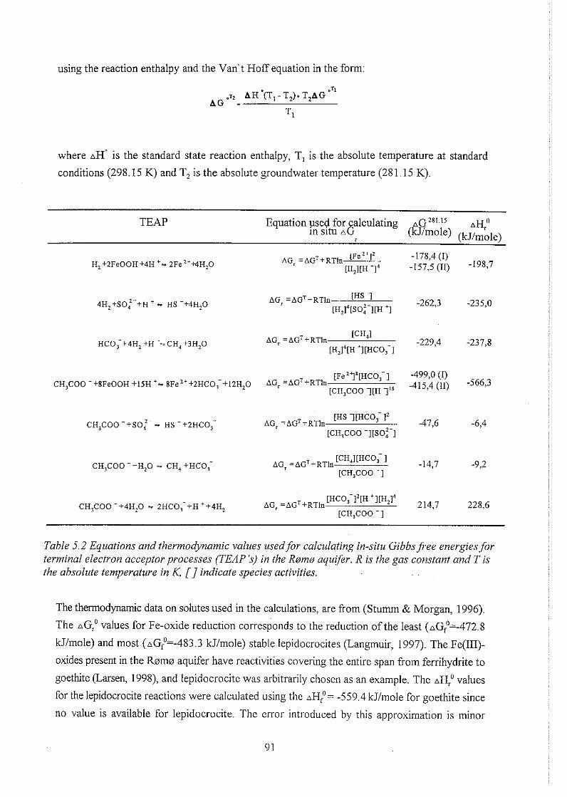
using the reaction enthalpy and the Van't Hoff equation in the form:
where AH" is the standard state reaction enthalpy, TI is the absolute temperature at standard
conditions (298.15 K) and T, is the absolute groundwater temperature (281.15 K).
TEAP Equation used for calculating A G ' ~ ' . ' ~ AH," In situ AG (kJ/mole) (kJ/mole)
AG, = A G ~ + R T ~ ~ [ ~ e ' * ] ~ -178,4 (1)
[H21[H *I4 -157,5 (11) -19837
~H,+so:-+H ' - HS -+4H,O AG, =AGT+RTln IHS ' -262,3 -235,O
[H,I~[~O:-I[H 'I
AG, =AG' +RTln [CH,I
HC0;+4H, +H +-CH4+3H,O -229,4 -237,8 [H2l4[H +I[HCO,-l
[ F ~ " ] " [ [ H C O , ~ -499,O (1) CH,COO -+8FeOOH +15H +- ~ F ~ ' * + ~ H C O ; + I ~ H , O AG, = A G ~ + R T ~ ~
[CH,COO 7[H ']'* -415,4 (11) -56633
[HS 7[HCO; 1' CH,COO - + S O : 3 HS -+2HCO; AG, = b G T + R ~ l n -47.6 -6,4
[CH,COO -][SO:-]
CH,COO -+H,O - CH, +HCO,-
AG, = A G ~ + R T I ~ [HCO,-I1[H *l[H,14 214r7
CH,COO -+4H,O 9 ZHC0,-+H ++4H, 228,6 [CH,COO - ]
Table j.2 Equations and thermodynamic values used for calculating in-situ Gibbs free energies for terminal electron acceptor processes (TEAPS) in the Rsmo aquifer. R is the gas constant and T is the absolute temperature in K, [ I indicate species activities.
The thermodynamic data on solutes used in the calculations, are from (Stumm & Morgan, 1996).
The AG: values for Fe-oxide reduction corresponds to the reduction of the least (AGP=-472.8
kJ/mole) and most (AGP=-483.3 kJ/mole) stable lepidocrocites (Langmuir, 1997). The Fe(II1)-
oxides present in the b m s aquifer have reactivities covering the entire span from ferrihydrite to
goethite parsen, 1998), and lepidocrocite was arbitrarily chosen as an example. The A&' values
for the lepidocrocite reactions were calculated using the AH:= -559.4 kJ1mole for goethite since
no value is available for lepidocrocite. The error introduced by this approximation is minor
because the effect of AH is small for small temperature differences, and also the temperature effect
on nGT is small. The main temperature effect comes from the second part of the equation.
The calculations of in situ Gibbs free energies were performed using the concentrations of Fe2',
CH, and SO:' measured in July 1997. The HCO; activities were calculated by PHREEQC
(Parkhurst & Appelo, 1997) from TIC and pH values measured in July 1997. The H, concentra-
tions measured in March 97 were used for location 8 and 10. For location 3 the average of the H,
concentrations measured in March and July 1997 were used. The acetate concentrations measured
in July 1997 were used for location 8 and 10 and the average of the concentrations measured in
1996 for location 3. As for the calculation of acetate turnover rates (section 2.5.3), narrow peaks
in the acetate concentration were neglected. Activity and complexion corrections were made by
entering the molar concentrations in PHREEQC (Parkhurst & Appelo, 1997), using the
PHREEQC database with values for acetate complexion added from the MINTEQ database
(Westall, Zachary & Morel, 1976). The concentrations of cations other than Fe2' used in
PHREEQC (Parkhurst & Appelo, 1997) calculations were those measured in 1996. The
concentrations of these cations are generally quite constant in the Ram aquifer and they have only
intluence on the complexion and activity corrections. C1- was adjusted to achieve electroneutrality.
The concentrations of S(I1) were not measured, since they are at or below the detection limit of
1 pM (Jakobsen, 1995). Accordingly the concentration of S@) was set to 1 pM in all samples and
the concentration of HS- was calculated with PHREEQC (Parkhurst & Appelo, 1997). If the
actual concentrations of S(II) were lower than 1 pM, then the AG, for sulfate reduction is slightly
more negative (higher energy yield) than calculated here. However, since the concentration of HS-
only enters into the logarithmic equations once, very large changes in the HS' concentration are
necessary to seriously affect AG, for sulfate reduction. Even a 100 fold decrease in the HS-
concentration would only increase the energy available for sulfate reducers by -2.7 kJImole H, and
-10.8 Wmole acetate, which is minor compared to the differences between the various TEAP's
under most conditions. The calculated in situ Gibbs free energies are shown in figure 5.3.
The suppression of CO, reduction by the presence of sulfate is consistent with the in situ AG,
values shown in figure 5.3. In all the samples, where sulfate is present, the AG, for CO, reduction
is zero or positive, and CO, reduction can therefore not occur at the H, concentrations measured
in the sulfate reducing zone. It is more difficult to explain, why methane production from acetate
is being suppressed. Sulfate reduction has a much larger energy yield per mole acetate than
methane production (-70 kJ/mole acetate and -30 kJImole acetate respectively). However, the
AG, for acetate fermentation is always n e g a t i v e < f 1 5 ~ ~ ! m @ a c e t ~ ~ ~ i ) h n d appears to be
completely unrelated to where the process occurs (figure 4.16). The highest energy yield is
actually found in the sulfate reducing zone, where the bulk of the acetate is turned over oxidatively
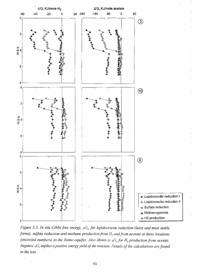
AG, KJlmole H, AG, KJlmole acetate
-60 -40 -20 0 20 -240 -160 -80 0 80
+ Lepidocrocite reduction I
o Lepidocrocite reduction II
-is Sulfate reduction
Methanogenesis
w H2 production
Figure 5.3. In situ Gibbsfree energy, AG, for lepidocrocite redtiction @east and most stable
forms), sulfate reduction and methane productionj?om H, and from acetate at three locations
(enc~rcled numbers) in the Romo aqtrqer. Also xhown IS AG, for H, prouZlctzon from acetate.
Negative AG, implies a positive enera yield ofthe reaction. Details ofthe calct~lations are found
in the text.
(figure 4.17). This is somewhat puzzling, since the whole concept of competitive exclusion of
redox processes is based on the ability of the more favourable TEAP to keep the concentration
of e.g. hydrogen or acetate down to a level, where the energy yield of other, less favourable,
TEAP's becomes too low for these processes to occur &ovley et al. 1982; Chapelle & Lovley,
1992; Lovley & Phillips, 1987).
The occurrence of CO, reduction is not easily explained from the calculated AG, values (figure 5.3)
either. While the AG, values for CO, reduction are generally slightly more negative in the parts of
the aquifer, where the process takes place at appreciable rates (below 2 m.b.s. at location 3, below
3 m.b.s. at location 10 and below 4 m.b.s. at location 8), there are no parts of the aquifer, where
they are < -4 Wmole Hz. While it can perhaps not be ruled out completely, that CO, reduction
could occur at such a low AG,, much higher threshold levels have been found by others. (Schulz
& Conrad, 1996) reported a threshold level for CO, reduction (at 4 "C) of -7 kJImole H,,
(Hoehler, 1998) reported a threshold level of -10 to -15 idlmole Hz in Cape Lookout Bight
sediment.
For the reduction of Fe(I1I)-oxides, an inverse relationship is found between the site, where
Fe(m)-oxide reduction is most energetically favourable (location 3) and the site where the highest
concentrations of Fez+ are found (location 8) in the upper part of the aquifer (figures 5.3 and 4.5).
Since the rates of sulfate reduction and methane production are much higher at location 3 than at
location 8 (figure 4.15 and 4-16), this cannot be due to a rate limiting availability of reactive
organic matter at location 3. Rather the Fee-oxides present at location 8 must be more reactive
than those present at location 3. In conclusion it is not possible to obtain usehl information from
the calculated AG, values for lepidocrocite reduction, since the stability of the Fe(1II)-oxides
present is unknown and apparently varies a lot between the different sampling locations. Apart
from mineral stability, the most important factor controlling AG, for Fe(I1I)-oxide reduction in the
Rsms aquifer is the pH, as indicated by the large increase in AG, for lepidocrocite reduction
occuning around 4 m.b.s. at location 3 and around 3 m.b.s. at location 10. The concentration of
Fe2+ also has a large effect, as indicated by the high AG, values for lepidocrocite reduction found
at all but the shallowest depth at location 8.
5.3 Dynamics of H, and acetate and the significance of their concentration levels
The lack of correlation between the measured in situ rates of redox processes (figure 4.15, 4.16
and 4.17) and their energy yields (figure 5.3), raise several questions about the cycling of H, and
acetate in sediments and the significance of their concentration levels.
The very low energy yield for CO, reduction, even in parts of the aquifer where the rate
measurements indicate appreciable rates, strongly suggests, that a large part of the CO, reduction
takes place within micro niches containing much higher Hz concentrations or by interspecies
hydrogen transfer between juxtaposed bacteria, as proposed by (Conrad et al. 1985; Thiele &
Zeikus, 1988). The juxtaposition arrangement might be thought of as a micro environment with
a higher Hz concentration between the cell walls of two bacteria. Accordingly, the two
phenomenons have the same effects, and, for the sake of simplicity, the term micro niches will be
used in the following to describe them both
Since the energy yield for CO, reduction at the bulk water Hz concentration is too low for the
process to occur, another TEAF', e.g. Fe(II1)-oxide reduction, must control the bulk water H,
concentration in the h m s aquifer, even when methane production actually is the dominating
TEAP. This seriously invalidates the whole concept of using Hz concentrations as indicator for the
TEAP as proposed by (Lovley & Goodwin, 1988). f&ovley & Goodwin, 1988) actually discussed
the possible influence that micro niches might have on the concept, but concluded, that the H,
concentration in the bulk sediment would be unaffected, as long as just a minor fraction of the Hz
is turned over there. This is theoretically correct, but only if one TEAP is active at a time, which
is not always the case (e.g. Canfield et al. 1993; Postma & Jakobsen, 1996, this study).
In conclusion, the concentration of hydrogen might still be used as an indicator of the dominant
TEAF', but the obtained results will only be reliable in sediments, where one TEAP dominates
completely. Moreover, recent studies (Hoehler, 1998) have shown, that the Hz concentration in
sediments depends not only on the TEAF', but also on other factors affecting the AG, values
(temperature and the concentrations of the involved species), as would be expected, if the bacteria
keeps the H, concentration as close to thermodynamic equilibrium as biologically possible. Rather
than using empirically defined concentration ranges, as those proposed by (Lovley & Goodwin,
1988; Chapelle et al. 1995), the actual in situ A G ~ values for the different TEAP's should be
calculated and compared to the expected threshold levels for the TEAP's. Still, where possible,
the diagnosis of TEAP is best made by measuring the rates directly.
If CO, reduction in the Ram aquifer occurs within micro niches, one might ask, why the process
does not take place at appreciable rates everywhere in the aquifer? A possible answer is, that other
bacteria, e.g. Fe(III)-oxide reducing and sulfate reducing, are able to outcompete the methanogens
for Hzinside the micro niches in some parts of the aquifer, but not in others. For sulfate reducers
this is easy to understand. Sulfate is present in millimolar concentrations and diffusion will
therefore rapidly replace any sulfate, that might be reduced within micro niches. Accordingly, the
only competitive advantage that methanogens could have over sulfate reducers, even in micro
niches, would be due to a size exclusion of the rather large sulfate reducing bacteria (cell lengths
of 0.9-11 pm according to (Widdel, 1988)). (McMahon & Chapelle, 1991) proposed, that sulfate
reducers were excluded kom aquitards because of the small pore siie, whereas fermenting bacteria
were not. However, to my knowledge, a similar phenomenon has not been reported to be
important in the competition between methanogens and sulfate reducers.
In some sulfate free parts of the aquifer, another redox process is apparently also able to prevent
CO, reduction within micro niches. This redox process could be Fe(II1)-oxide reduction, but this
requires, that all micro niches contain Fe(II1)-oxides in these parts of the aquifer. The occurrence
of CO, reduction in other parts of the aquifer (within micro niches) must then be due to a rate
limiting low reactivity of the Fe(II1)-oxides present there andlor a more uneven distribution of
them. I
Alternatively, the measured Hz concentrations are significantly lower than the actual concentra-
tions, but there is no evidence to support this. (Frank, 1996) measured H, concentrations at
location 3, using a completely different method (collection of gas from the headspace of sealed
micro-wells, installed in the aquifer) and found concentrations similar to those measured in this
study by the bubble stripping method (section 2.4).
The ~ G ~ v a l u e s for sulfate reduction from Hz are also quite low (-7 to -10 k.J/mole H,, figure 5.3).
This could indicate, that sulfate reduction from H, also takes place within micro niches. The
concentration of hydrogen would then be controlled by another redox process, e.g. Fe(II1)-oxide
reduction, also in the sulfate containing parts of the aquifer. In support of this, the concentration
of hydrogen does not increase significantly at the depth of sulfate depletion at location 10 and 8,
whereas (Jakobsen, 1995) measured higher Hz concentrations (about 1 nM rather than 0.2-0.4
nM) in some sulfate containing parts of the aquifer than those found in this study . However,
threshold values for CO, reduction as low as 7 Wmole H, at 4 "C have been reported (Schulz &
Conrad). Ifsulfate reduction from Hz can occur at a similar low energy yield, the H, concentration
could be controlled by sulfate reducers in the sulfate containing parts of the aquifer.
For all TEAP's, the energy yield is appreciably lower for the reaction involving acetate than for
the reaction involving H, (figure 5.3). This is true when the comparison is made on a mole
substrate basis, as in figure 5.3, but also when the comparison is made on a mole electron acceptor
basis. The in situ AG, value for oxidation of acetate to CO, + H, (figure 5.3) is negative in all but
a single sample, which means that oxidation of acetate to CO, + Hz is always energetically
favourable. Accordingly, all the TEAPs has a larger energy yield per mole electron acceptor from
acetate than from Hz. Either way we may look at it, the redox processes involving acetate are
further fiom thermodynamic equilibrium than those involving Hz. This indicates, that the acetate
utilizing bacteria requires a larger energy yield than the hydrogen utilizing bacteria. The reason for
this is perhaps, that acetate is a much larger and more complex molecule than Hz. It is also evident,
that methanogenic bacteria can keep the concentration of acetate much closer to thermodynamic
equilibrium than the sulfate reducing bacteria, since the energy yield for sulfate reduction from
acetate is more than 3 times higher than the energy yield at which acetate fermentation takes place
(figure 5.3 and 4.16).
As shown in the previous section, the suppression of methane production from acetate in parts of
the aquifer is not due to a low acetate concentration or to a low energy yield of the process . Other
studies have however shown lower acetate concentrations in sulfate reducing than in methane
producing parts of a sediment. (Kuivila et al. 1988) found that the acetate concentration was 10-15
pM in the sulfate reducing part ofLake Washington sediment, and 30-40 pM in the methanogenic
part of the sediment. Lower acetate concentrations have also been reported in Fe(II1)-oxide
reducing parts of an aquifer (0.5-2.0 pM) than in sulfate reducing parts of the aquifer (2.0-3.0
pM) (Chapelle & Lovley, 1992).
The acetate concentration has, however, only a limited effect of the energy yield of the TEAP's.
The change in A G ~ for sulfate reduction and methane production from acetate accomplished by the
2-4 fold change in the acetate concentration between ditferent TEAP s, that was found by (Kuivila
et al. 1988; Chapelle & Lovley, 1992), is only a few kJimole acetate. While it perhaps cannot be
ruled out completely, such a small change in AG, seems unlikely to inhibit a redox process.
Possibly the methanogenic bacteria are not being outcompeted for acetate by sulfate reducers or
Fern-oxide reducers, but the low Hz concentration maintained by these bacteria causes them to
switch their metabolism from fermentative to oxidative cleavage of acetate, where the electrons
are released in the form of Hz rather than as CH,. Studies in well defined cocultures of acetate
consuming rnethanogens and Hz consuming sulfate reducers have demonstrated the ability of
certain strains of acetogenic methanogens to switch their metabolism from fermentative to
oxidative cleavage of acetate, where the electrons are presumably released in the form of Hz
(Phelps et al. 1985). This switch took place, when the Hz concentration was kept down by sulfate
reducers.
There is also evidence for the occurrence of the process in natural environments. (Achtnich et al.
1995) investigated the turnover of acetate and Hz in a methanogenic paddy soil and demonstrated,
that addition of sulfate or Fe(II1)-oxides to the sediment resulted in large decreases in the Hz
concentration while the acetate concentration remained constant, except from a temporary
increase, when sulfate was added. Inhibition experiments with chloroform showed, that the sulfate
reducers present in the sediment could not utilize acetate directly, and that methanogens switched
at least partly from methane production to Hz production from acetate, when sulfate or Fe(II1)-
oxides was added to the sediment.
In general there is a good agreement between the sites, where high Hz concentrations were
measured (figure 4.10) and the sites, where methane production from both H, and acetate occurs
at appreciable rates (figure 4.16). The calculated in situ AG, values (figure 5.3) show, that H21C02
production from acetate is more energetically favourable than CH, production from acetate in all
parts of the aquifer, where low methane production rates and a high respiration index was
measured (above 2 m.b.s. at location 3, above 3 m.b.s. at location 10 and above 4 m.b.s. at
location 8). In contrast, the CH, production from acetate is generally more favourable, or the two
processes are equally favourable, in the parts of the aquifer, where high methane production rates
and a low respiration index was measured.
The AG, values at location 10 deviates a bit from this general picture. The reason for this is not
known, but it is possible, that the concentration of H, changed substantially here between March
1997, when the H, concentrations were measured and July 1997, when the rates were measured.
The low concentrations of methane and the occasional presence of sulfate in this part of the
aquifer (figure 4.5) indicate, that location 10 is situated very close to the point, where methane
production replaces sulfate reduction along this flowline. Accordingly the H, concentration could
fluctuate considerably here, depending on whether sulfate reduction or methane production is the
main TEAP.
In conclusion, the H, concentration level could be the main control on methane production from
acetate by causing a switch in the metabolism of acetate utilizing methanogens from the
production of methane to the production of hydrogen, when the hydrogen concentration is low
enough to make this energetically favourable. In the sulfate containing parts of the aquifer, the H2
produced this way could be consumed by sulfate reducers andlor Fe(II1)-oxide reducers, and in
the parts of the aquifer that are free of sulfate, the Fe(II1)-oxide reducers could consume the
hydrogen. H, production from acetate could also explain the oxidation of acetate in methanogenic
parts of the aquifer, but since it requires a low hydrogen concentration, the possible occurrence
of this process does not remove the need of an electron acceptor other than CO, (methane
production) in sulfate free parts of the aquifer. If most of the oxidative decomposition of acetate
is shunted through hydrogen, an explanation is also provided for why sulfate reduction with
acetate is as far as 70 kJImole acetate from thermodynamic equilibrium, since the energy yield
would then have to be split between two bacteria: one that produces H, from acetate and one that
consumes the H, (a sulfate reducer).
Alternative explanations for the high RI in parts of the aquifer are of course also possible. One
such explanation could be, that the methanogenic bacteria are able to utilize acetate only by
cometabolism with another substrate like hydrogen. The high respiration index in parts of the
aquifer could then be explained by the outcompetition of methanogens for hydrogen (figure 4.16
and 4.17). However, this would be completely without precedence in the literature, at least to my
knowledge. Another possibility could be the inhibition of acetate utilizing methanogens by a
substance present in parts of the sediment. Inhibition of methane production from acetate by high
concentrations of sulfide has been demonstrated (e.g. Gunnarsson & Ronnow, 1982), but in the
b m 0 aquifer this possibility can be excluded, because of the very low sulfide concentration.
Finally the acetate utilizing methanogens could be inhibited by a lack of an essential nutrient like
N or S, but it seems somewhat unlikely, that such a lack of nutrient would not affect the sulfate
reducers and Fe(II1)-oxide reducers as well.
Whde the differences between the acetate concentrations in zones with different TEAP's are minor
(Kuivila et al. 1988; Chapelle & Lovley, 1992) or absent (this study), the concentrations of acetate
found in different sediments with the same TEAP varies up to four orders of magnitude (review
of acetate concentrations in sulfate reducing marine sediments by (Sansone & Martens, 1982)).
Also studies from polluted aquifers have shown concentrations of acetate and other fatty acids
covering a span of several orders of magnitude, but with no correlation to the concentration of
hydrogen (Vroblesky et al. 1997). In conclusion, no information, about which TEAP dominates,
can be obtained from acetate concentrations
/ It is interesting, that acetate concentrations can vary so much within the same TEAP, whereas the
H2 concentration is much more tightly controlled by the redox processes. At least two factors
might be responsible for this. Firstly, the concentration of hydrogen is orders of magnitudes lower
than the concentration of acetate (figure 4.10) and for this reason, the hydrogen pool is turned
over much faster. To illustrate this point, the turnover times of H, and acetate in the b m 0 aquifer
were calculated from the rates measured in July 1997. The turnover of Hz by other redox
processes than methane production has not been measured directly. Since most of the methane
production occurs via the CO, reduction pathway (figure 4.16), it was conservatively assumed,
that the other redox processes occurred equally via Hz and acetate, and the Hz turnover time was
approximated from the measured rates of CO, reduction and acetate oxidation. The results are
shown in figure 5.4.
While the pool of H2 is turned over in less than 1 minute in many parts of the &m aquifer, the
pool of acetate is only turned over every 5-500 hours. This implies, that an increased production
of hydrogen will very rapidly increase the concentration of hydrogen significantly and thus
stimulate the growth of hydrogen utilizing bacteria. For acetate the link from production to
consumption works much slower because of the larger pool size. Moreover, since 4 moles of H,
but only one mole of acetate is needed for the reduction of one mole sulfate or production of one
mole methane, a change in the Hz concentration has a four times larger relative effect on the AG~'s
than does a s i i la r change in the concentration of acetate. A 100 fold increase in the concentration
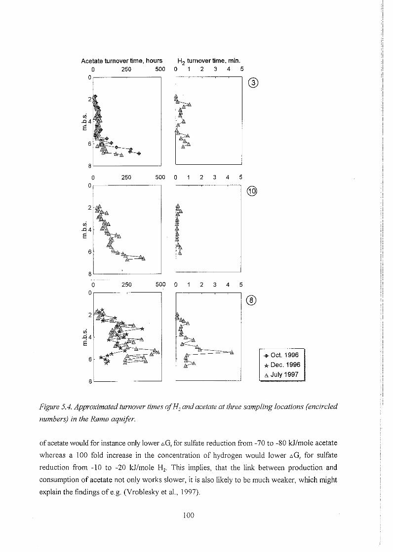
Acetate turnover time, hours 0 250 500
H2 turnover time, min. 0 1 2 3 4 5
Figure 5.4. Approximated tzimover times o fH , andacetate at three .sampling locations (encircled
numbers) in the Rsm0 nqzlyer.
of acetate would for instance only lower AG, for sulfate reduction from -70 to -80 kJlmole acetate
whereas a 100 fold increase in the concentration of hydrogen would lower AG, for sulfate
reduction from -10 to -20 kJImole H,. This implies, that the link between production and
consumption of acetate not only works slower, it is also likely to be much weaker, which might
explain the findings of e.g. (Vroblesky et a]., 1997).

The much larger turnover time of acetate also has the implication, that microniches with higher
concentrations of acetate cannot form in homogeneous sediment at steady state. Diffusion and (in
aquifers) advective transport will effectively level out any concentration differences, that might
develop): on a micro scale. On the other hand, higher acetate concentrations might be found in
areas with a horizontal extension of centimetres to metres, if the redox processes are not at steady
state. Possibly this is the reason for some of the local peaks and temporal variations in the acetate
concentration in the RQm aquifer (figure 4.8). In geologically diverse flow systems, large
differences in the acetate concentration might also exist between the different types of sediment,
as described by (McMahon & Chapelle, 1991).
To complete this minireview of acetate cycling in sediments, it should be mentioned, that a
mechanism for acetate turnover in methanogenic sediments, that is almost opposite the one
proposed here, has previously been proposed by (Sansone & Martens, 1982). In an attempt to
explain the oxidation of acetate in sulfate free methanogenic sediment from Cape Lookout Bight,
(Sansone &Martens, 1982) proposed, that acetate was oxidized to Hz by sulfate reducers, when
sulfate was absent and the H, subsequently used by methanogens. Since the CO, reduction rate
is higher than the acetate oxidation rate in Cape Lookout Bight (Sansone & Martens, 1982; Crill
& Martens, 1986) this is indeed a possibility here. However, (Sansone & Martens, 1982) used U-
14C-acetate, so perhaps some of the apparent acetate oxidation was actually isotope exchange
(section 1.4).
Moreover, in the RQm aquifer, the acetate oxidation rate is often much higher than the CO,
reduction rate, which already excludes this explanation for the occurrence of acetate oxidation in
sulfate free parts of the aquifer. Active sulfate reducers are however present below the depths of
sulfate depletion, as indicated by the rapid turnover of injected 35S0,2- in many samples with a low
sulfate concentration. Moreover, the turnover of injected 35S0,2- tracer was extremely high (up
to 80 % within 24 hours) at the exact same site, where the highest acetate oxidation rates were
measured. Therefore, a connection between acetate oxidation and sulfate reducers in the sulfate
free part of the aquifer cannot be excluded. However, hydrogen produced from acetate by sulfate
reducers could not be consumed by methanogenic bacteria, as suggested by (Sansone & Martens,
1982).
5.4 Controls on the methane concentration in deep aquifers
As discussed in the previous sections, the availability of reactive organic matter and the
competition with other redox processes are the main factors controlling, whether methane is
produced in appreciable amounts in aquifers. If the input of reactive organic matter from the soil
zone is large, then methane might form shortly below the groundwater table in a shallow aquifer,
but only after the oxygen, nitrate and sulfate present in the infiltrating water has been used up
(figure 4.5 and 4.8). In contrast, the presence of Few)-oxides only prevents methane production,
ifthe Fe(m)-oxides are reactive enough. The amount of methane, that forms in shallow aquifers
is therefore mainly controlled by a mass balance between the amount of reactive organic carbon,
leaching from the soil zone, and the amount of other, competing, electron acceptors, that are
present in the infiltrating water.
In deeper aquifer systems, the same two factors - availability of reactive organic matter and
competition with other TEAP's - will also control the formation of bacterial methane. But in
contrast to shallow unconfined aquifers, it is much more likely, that organic matter, deposited with
the sediment, is the main electron donor in deep, confined aquifers. (Simpkins & Parkin, 1993)
for instance reported that the methane in a confined aquifer in central Iowa is formed from a high
amount of organic matter in the sediment, originating from the burial of a forest during the last
glaciation. Also, isotopic analysis show, that the methane and DIC in a confined aquifer in
Southern Ontario is formed £tom old SOM (sedimentary organic matter) rather than from organic
matter, leaching from the soil zone (Aravena & Wassenaar, 1993). The formation of methane in
deep aquifers is therefore mainly controlled by the amount and reactivity (age) of the organic
matter deposited with the sediment.
How high concentrations of methane, that builds up in the water, is controlled, not only by the rate
of methane production, but also on the residence time of the water. (Grossman et al. 1989)
measured up to 28.8 mM CH, in a deep aquifer in Texas, which is about 50 times more than the
highest concentration found in the shallow h w aquifer.
Another factor, that might influence the concentration of methane in aquifers, is methane
oxidation. However, this study has shown, that methane oxidation rates are very low in the
transition zone between sulfate and methane in the shallow h m s aquifer (figure 4.19). A likely
explanation is, that the energy yield of methane oxidation with sulfate as electron acceptor is
below the threshold level required for the process to occur. The in situ AG, value for the process
is approximately 40 kJ/mole. If methane oxidation coupled to sulfate reduction occurs via a
reversal of the CO, reduction pathway, as proposed by (Hoehler et al. 1994), the reaction might
be written as two half reactions:
1) CH, + 3 H20 -> HCO; + H' + 4 H,
2) 4 H, + SO:. + H+ -> HS- + 4 H,O
Four hydrogen molecules are involved in the reaction, and two bacteria (a methanogenic and a
sulfate reducing) has to share the available energy between them. This means, that only 5 KJImole
H2 is available to each bacteria, which is below the threshold values reported in the literature for

CO, reduction (Schulz & Conrad, 1996; Hoehler, 1998). It is therefore consistent with
thermodynamic considerations, that methane oxidation with sulfate as electron acceptor does not
occur in the Rams aquifer.
The low energy yield for methane oxidation with sulfate as electron acceptor is mainly a result of
the low concentration of both sulfate and methane in the transition zone. In marine sediments, both
methane and sulfate is present in concentrations of up to several rnM in the transition zone,
whereas their concentrations rarely exceeds 0.1 mM in the transition zone in the R a m aquifer.
Moreover, in marine sediments, methane oxidation seems to stop, when a methane concentration
of-0.2 mM is reached (Whiticar & Faber, 1986). The lack of methane oxidation with sulfate as
electron acceptor is therefore also consistent with previous findings from marine sediments. The
low concentrations of sulfate and methane are due to a lower input of sulfate than in marine
sediments, but also to the lower rates of sulfate reduction and methane production (table 5.1) and
to the different modes of transport that dominates (diffusion in marine sediments, advective
transport in aquifers).
In deep, contined aquifers, the flow conditions are often very different from shallow aquifers, and
it is possible, that the conditions necessary for methane oxidation could be met. Higher
concentrations of methane might form due to the long residence time of the water, and if this
methane comes in contact with a possible electron acceptor, methane oxidation is likely to occur.
One situation, that could lead to such a contact, is formation of methane within layers with a low
permeability. If water containing sulfate, nitrate or oxygen flows in more permeable layers,
di is ion could transport large amounts of methane into the moving water, where it might act as
an electron donor for the reduction of oxygen, nitrate and sulfate in that order.
In contrast, oxygen, nitrate and sulfate will not come near methane containing water in
homogeneous deep flow systems, since the redox zones often have a horizontal extension of
several kdometres in deep aquifers. Mixture of sulfate and methane containing water by diffusion
over such distances will be extremely limited. Accordiigly, if the concentration of sulfate in water,
infiltrating an aquifer, is raised, it cannot be expected, that methane will become an important
electron donor for sulfate reduction in a homogeneous flow system. Rather, sulfate reduction will
replace methane production, when high sulfate water enters the previously methanogenic part of
the aquifer, as illustrated in (figure 4.8). Since the rate of organic matter decomposition seems to
be largely independent ofwhether sulfate reduction or methane production is the TEAF' (table 5.1
and figure 5.3), the amount of sulfate, that the organic matter in the sediment is able to reduce,
will be closely related to the amount of methane, that it was able to form, when methane
production was the T E N . A good approximation of a methanogenic aquifer's ability to reduce
sulfate can therefore be obtained, by simply measuring the concentration of methane in the water.
6 Conclusions
The methane in the h m aquifer is produced mainly by the CO, reduction pathway, but acetate
fermentation is a more important process than in deep aquifers. The rate of methane production
as well as the relative importance of CO, reduction and acetate fermentation varies highly over
depth and between sampling locations, despite the apparent homogeneity of the sediment. CO,
reduction accounts for more than 90 % of the produced methane, where the highest rates are
measured, but only 10-80 % elsewhere. The significant contribution of acetate fermentation to
methane production results in methane more depleted in deuterium than methane from deep
aquifer systems. The rates of methane production are 1-3 orders of magnitude lower than those
measured in most marine sediments, but comparable to the rates measured in some lake sediments.
These differences reflects the availability of reactive organic matter.
From mass balance considerations it appears, that most of the organic matter being decomposed
in redox processes must come &om the soil zone, and DOC profiles indicate, that a lot of it must
be transported on a colloidal form. Factors likely to influence the load of organic carbon into the
aquifer, are the residence time of water in the unsaturated zone and the type of vegetation.
There is a distinct separation between methane production and sulfate reduction. When sulfate
enters previously methane producing parts of the aquifer, sulfate reduction replace methane
production, whereas methane is readily formed in previously sulfate reducing parts of the aquifer,
when sulfate is no longer present. The rate of organic matter decomposition is largely independent
of whether sulfate reduction or methane production is the TEAP (Terminal Electron Accepting
Process).
Fe(II1)-oxides are present everywhere in the aquifer, and Fe(II1)-oxide reduction and sulfate
reduction occurs concurrently. In sulfate fiee parts of the aquifer, another redox process, possibly
Fe(II1)-oxide reduction, occurs concurrently with methane production. This redox process
strongly suppress methane production in some sulfate free parts of the aquifer, but not in others.
In contrast to marine sediments, methane oxidation coupled to sulfate reduction in the transition
zone between sulfate and methane is an ins idcan t process in the Rams aquifer. This most likely
reflects the much lower concentrations of sulfate and methane.
The hydrogen concentration reflects the dominant TEAP to some degree, but the energy yield for
CO, reduction at the bulk water hydrogen concentration is so low, that CO, reduction must take
place within micro niches with higher H2 concentrations or by interspecies hydrogen transfer
between juxtaposed bacteria. The H, concentration in the bulk water must therefore be controlled
by another redox process, even when CO, reduction is the dominant process. In this situation, the
concentration of hydrogen cannot be used to determine the dominant TEAP. The concentration
of acetate is completely unrelated to the TEAP Calculations of the energy yield for acetate
turnover show, that suppression of acetate fermentation in parts of the aquifer cannot be due to
a low energy yield of the process, which is the traditional explanation. It is suggested, that the
concentration of hydrogen controls the turnover of acetate by causing acetogenic methanogens
to swich their metabolism &om methane production to production of hydrogen from acetate, when
the hydrogen concentration is low enough to make this energetically favourable.
References
Abram, J.W. & Nedwell, D.B. (1978) Inhibition of methanogenesis by sulfate-reducing bacteria competing for transferred hydrogen. Arch. Microbial. 11 7, 89-92.
Achtnich, C., Scbuhmann, A., Wind, T., & Conrad, R. (1995) Role of interspecies H, transfer to sulfate and femc iron-reducing bacteria in acetate consumption in anoxic paddy soil. FEbfSMicrob. Ecol. 16,61-70.
Alp& M.J. & Reeburgh, W.S. (1988) Carbon and hydrogen isotope fractionation resulting fiom anaerobic methane oxidation. Glob. Biogeochem. Cyc 2, 279-288.
Aravenh R & Wassenaar, L.I. (1 993) Dissolved organic carbon and methane in a regional confined aquifer, southern Ontario, Canada: Carbon isotope evidence for associated subsurface sources. Applied Geochemistry 8,483-493.
Aravena, R., Wassenaar, L.I., &Barker, J.F. (1995) Distribution and isotopic characterization of methane in a co&ied aquifer in southern Ontario, Canada. J Hydrology 173.5 1-70.
Aravena, R., Wassenaar, L.1, & P l m e r , L.N. (1995) Estimating 14C groundwater ages in amethanogenic aqnlfer. CVaterReso~rrces Research 31,2307-23 17.
Barker, J.F. &Fritz, P. (I 981) The occurrence and origin of methane in some groundwater flow systems. Can. J Earth Sci. 18, 1802-1816.
Bates, T.S., Lamb, B.K., Gnentn; A,, Digoon, J., & Stoiber, RE. (1 992) Sulfur emissions to the atmosphere from natural sources. J Amos. Chem. 14,3 15-337.
Berner, R.A. (1980) Early diagenesis: A theoretical approach. Princeton, New Jersey (USA).
Berner, R.A. (1980) A rate model for organic matter decomposition during bacterial sulfate reduction in mmine sediments. Colloques Intemationaux d~r C. N. R. S. Biogeochemie de la matiire organique a ?interface eau-sediment marin. 293, 35-44.
Bemer, R.A. (1985) Sulphate reduction, organic matter decomposition and pyrite formation. Phil. Trans. R. Soc. Lond. A 315,25-38.
Bjerg, P.L., Jakobsen, R., Bay, H, Rasmussen, M., Albrectsen, H., & Christensen, T.H. (1997) Effects of sampling well wnstluction on H, measurements made for characterization of redox conditions in a contaminated aquifer. Environ. Sci. Tech. 31,3029-303 I.
Blair, N.E. & Robert, C.A. (1995) Anaerobic methane oxidation on the Amazon shelf Geoc. Cosmoc. Acta 59, 3707-37 15.
Buchardt, B. (1998) Geological Institute, University of Copenhagen. Personal communication
Canfield, DE.. Thamdmp, B., & Hansen, J.W. (I 993). The anaerobic degradation of organic matter in danish coastal sediments: Iron reduction, manganese reduction and sulfate reduction. Geoc. Cosmoc. Acta 57, 3867-3883.
Chapelle, F.H. & Lovley, D.R. (1992) Competitive exclusion of sulfate reduction by Fe(II1)-reducing bacteria: A mechanism for producing discrete zones of hlgb-iron ground water. Ground Water 30,29-36.
Chapelle, F.H. & McMahon, P.B. (1991) Geochemistly of dissolved inorganic carbon in a coastal plain aquifer. 1 Sulfate from confiiing beds as an oxidant in microbial CO, production. J. Hydrology 127,85-I 08.
Chapelle, F.H., McMahon,P.B.,Dubrovsky, NM.,Fujii, R.F., Oaksford, E.T., & Vroblesky, D.A. (1995) Deducing the dislribution of terminal electron-accepting processes in hydrologically diverse groundwater systems. CVaterResorrrces Research 31,359-371
Christensen CV.(1994) EUogging og grundvandsmodellering p i h n w . Institute of Geophysics and Geology, University
of Aarhus. M.Sc. Thesis.
Chnstensen, D. & Blackbum, T.H. (1982) Tumover of 'dC-labelled Acetate in marine sediments. Marine Biology 71, 113-119.
Coleman, D.D., Liu, C., & Riley, K.M. (1988) Microbial methane in the shallow paleozoic sediments and glacial deposits of Illimois, USA. Chemical Geology 71,23-40.
Coleman,D.D., Risatti, J.B., & Schoell, M. (1981) Fractionation of carbon and hydrogen isotopes by methane-oxidizing bacteria. Geoc. Cosmoc. Acta 45, 1033-1037.
Conrad, R., Phelps, T.J., & Zeikus, J.G. (1985) Gas metabolism evidence in support of the juxtaposition of hydrogen-producing and methanogenic bacteria in sewage sludge and lake sediments. Appl. Environ. Microbiol. 50, 595-601
Crill, P.M. & M&ens, C.S. (I 986) Methane production form bicarbonate and acetate in an anoxic marine sediment. Geoc. Cosmoc. Acta 50,2089-2097.
Dauielson, L.G. (I 982) On the use of filters for distinguishmg between dissolved and particulate fractious in natural waters. WaterRes. 16, 179-1 82.
Devol, A.H. (1983) Methane oxidation rates in the anaerobic sediments of Saanich Met. Limnol. Oceanogr. 28, 738-742.
Devol, A.H. & Ahmed, S.I. (1 981) Are high rates of sulphate reduction associated with anaerobic oxidation of methane. iVarilre 291,407-408.
Felmy AR, Girvin DC, and Jenne EA. MTNTEQ (1 984) A computer program for calculating aqueous geochemical equilibria. U.S. Environm. Protection Agency. Athens.
Frind, E.O., Duyrusveld, W.H.M., Strebel, O., & Boettcher, J (1989) Simulation of nitrate and sulfate transport and transformation in the Fuhrberger Feld aqufe~, Hamover, Germany. In: Contaminant transport in groundwater. (Kobus & Kmzelbach. Ed.) pp 97-104, Bakema, Rotterdam.
Frind, E.O., Duynisveld, W.H.M., Strebel, O., & Boettcher, J. (1990) Modelling of multi-component transport with microbial transformation in groundwater: The Fubrberg case. WaterResources Research 26, 1707-17 19.
Gibson, G.R., Parkes, R.J., & Herbert, R.A. (1989) Biological availability and turnover rate of acetate in marine and estuarine sediments in relation to dissimilatory sulphate reduction. FEMS~bficrob. Ecol. 303-306.
G r d , WW., Wellsbury, P., Parkes, R.J., & Cappenberg, T.E. (1 996) Comparison of acetate turnover in methanogenic and sulfate-reducing sediments by radiolabeling and stable isotope labeling and by use of speciFic inhibitors: Evidence for isotopic exchange. Appl. Environ. Microbiol. 62,772-777.
Grossman, E.L., Cofhan, B.K., Fritz, S.J., & Wada, H. (1989) Bacterial production of methane and its influence on ground-water chemistry in east-central Tesas aquifers. Geology 17,495-499.
Gron, C., W m a a r , L., & Krog, M. (1996) Origin and smctures of groundwater humic substances from three Danish aquifers. Environment International 22,5 19-534.
Gunnarssoq L.A.H. & Rounow, P.H. (1 982) Interrelation between sulfate reducing and methane producing bacteria in coastal sediments with intense sulfide production. Marine Biology 69, 121 -128.
Harder, 3. (1997) Anaerobic methane oxidation by bacteria employing "C-methane uncontaminated with '4C-carbon monoxide. ibfarine Geology 137, 13-23.
Harvey, H.R., Fallou, R.D., & Patton, J.S. (1989) Methanogenesis and microbial lipid synthesis in anoxic salt marsh sediments. Biogeochemist~ 7, 11 1-129.

Hoehler, T.M. (1 998) Thermodynamics and the role ofhydrogen in anoxic sediments. University of North Carolina. Ph.d. dissertation. (The refered results will also be published in Geoc. Cosmoc. Acra, 62 (10) 1998).
Hoehler, T.M., Alperin, M.J., Albert, D.B., &Martens, C.S. (1 994) Field and laboratory studies of methane oxidation in an anoxic marine sediment: Evidence for a methanogen-sulfate reducer consortium. Glob. Biogeochem. Cyc. 8, 451-463.
Iversq N. & Blackbum T H (1981) Seasonal rates of methane oxidation in anoxic marine sediments. Appl. Environ. iMicrobio1. 41, 1295-1300.
Iversen, N. & Jorgensen, B.B. (1985) Anaerobic methane oxidation rates at the sulfate-methane transition in marine sediments from Kattegat and Skagerrak (Denmark), Limnol. Oceanogr. 30,944-955.
Iversq N., Oremland, R.S., & Klug, M.J. (1 987) Big Soda Lake (Nevada). 3. Pelagc methanogenesis and anaerobic methane oxidation. Limnol. Oceanogr. 32,804.-814.
Jakobsen R.(1995) Sulfate reduction, Fe-reduction and methanogenesis in groundwater. Department of Geology and Geotechnical Engineering, Technical University of Denmark. Ph.d. dissertation.
Jakobsen, R., Albrechtsen, H., Rasmussen, M., Bay, H., Bjerg, P.L., & Christensen, T.H. (1998) &concentrations in a landfill leachate plume ( G ~ d s t e d , Denmark) - in situ energetics of terminal electron acceptor processes. ES&T (m press)
Jakobsq R. & Postma, D. (1994) In situ rates of sulfate reduction in an aquifer @m, Denmark) and implications for the reactivity of organic matter. Geologv 22, 1 103-1 106.
Jakobsen, R. & Postma, D. (1998) SuLfate reduction, sulfide formation, Fe-reduction and methanogenesis: Rates, interactions, energetics and redoxzonation in a shallow unconsolidated sand aquifer, bm, Denmark. Geoc Cosmoc. Acta, (submitted).
Johansen, L. (1997) Redoxzonering i Grundvandszonen. Department of Geology and Geotechnical Engineering, Technical University of Denmark. M.Sc Thesis.
J~rgensen B.B. & Fenchel, T. (1 974) The sulfur cycle of a marine sediment model system. Marine Biology 24, 189-201
k g , G.M. (1984) Utilization of hydrogen, acetate, and "noncompetitive" substrates by methanogenic bacteria in marine sediments. Geomicrobiol J. 3,275-306.
Krzycki, J.A., Wollcin, R.H. & Zeikus, J.G. (1 982) Comparison of unitrophic and mixotophic substrate metabolism by an acetate-adapted strain ofMetanosarcina Barkeri. J. Bacteriol. 149, 247-254.
Kuida, K.M., Murray, J.W., & Devol, AH. (1 988) Methane production, sulfate reduction and competition for substrates in the sediments ofLake Washington. Geoc. Cosmoc. Acta 53,409-416.
Langnuir, D. (1 997) Aqueous environmentalgeochemisty, Prentice-Hall, Inc. New jersey.
Lansdown, J.M., Quay, P.D., & King, S.L. (I 992) CH, production via CO, reduction in a temperate bog: A source of "C-depleted CH* Geoc. Cosmoc. Acta 56, 3493-3503.
Larsen F. (1996) Pynte oxidation in a well field -processes controlling sulfate and nickel in groundwater. Geological Smey ofDenmark and Greenland and Department of Geology and Geotechnical Engineering, Technical University of Denmark. Ph.d. Dissertation
Larsen 0. (1 998) Reactivity of I r o n o oxides and I r o n 0 oxide reduction in a shallow aquifer. Department of Geology and Geotechnical Engineering, Technical University of Denmark. Ph.d. Dissertation.
Lovley, D.R. & Chapelle, F.H. (1 995) Deep subsurface microbial processes. Reviews of Geophysics 33,365-38 1
Lovley, D.R., Dwyer, D.F., & Klug, M.J. (1982) finetic analysis of competition between sulfate reducers and methanogens for hydrogen in sediments. Appl. Environ. Microbiol. 43, 1373-1379.
Lovley, D.R. & Goodwin, S. (1988) Hydrogen concentrations as an indicator of the predominant terminal electron-accepting reactions in aquatic sediments. Geoc. Cosmoc. Acta 52,2993-3003.
Lovley, D.R. & Klug, M.J. (1983) Sulfate reducers can outcompete methanogens at freshwater sulfate concentrations. Appl. Environ. ~Microbiol. 45, 187-192.
Lovley, DR. &Phillips, E.J.P. (1 987) Competitive mechanism for inhibition of sulfate reduction and methane production in the zone of femc uon reduction in sediments. Appl. Environ. Microbial. 53,2636-2641
Maburnoto, J. & Hanaki, K. (1 990) Sulfate reduction and methane production during degradation of organic materials in coastal sediment. J. Coil Engng. ~Vihon Univ. 31,7-18.
McMahon, P.B. & Chapelle, F.H. (1991) Geochemistry of dissolved inorganic carbon in a coastal plain aquifer. 2. Modelling carbon sources, sinks, and 6I3C evolution. J Hydrology 127, 109.335.
McMahon, P.B. & Chapelle, F.H. (1991) Microbial production of organic acids in aquitard sediments and its role in aquifer geochemistry. Natzrre 349,233-235.
Michelso~ A.R., Jacobson, M.E., Scranton, M.I., & Mackin, J.E. (I 989) Modelling the distribution of acetate in anoxic estuarine sediments. Limnol. Oceanogr. 34,747-757.
Nielsen, R.R. & Hoherjord, G. (1997) Methanogenesis in Aquifers. Radiotracer measurements in anoxic sediment Ram, Denmark. Institute for Geology and Geotechnical Engineering, Technical University of Denmark. M.Sci. Thesis.
Niewohner, C., Hensen, C., Kasten, S., Zabel, M., & Schulz, H.D. (1998) Deep sulfate reduction completely mediated by anaerobic methane oxidation in s e d i i t s of the upwelling area off Namibia. Geoc. Cosmoc. Acta 62,455-464.
Nissenbaum, A & Kaplan, I.R. (1972) Chemical and isotopic evidence for the in-situ origin of marine humic substances. Limnol. Oceanogr 17,570-582.
Novelli, P.C., Michelson, A.R., Scrantou, M.I., Banta, G.T., Hobbie, J.E., & Howarth, R.W. (1988) Hydrogen and acetate cycling in two sulfate-reducing sediients: Buzzards Bay and Yawn Cove, Mass. Geoc. Cosmoc. Acta 52, 2477-2486.
Omemland, R.S. (1 988) Biogeochemishy of methanogenic bacteria. In Biology ofanaerobic microorganisms (Zehnder, J.B. Ed.) pp 641-706, John Wiley & Sons, Inc. New York.
Oremland R.S., Marsh L.M., & Polcin, S. (1982) Methane production and simultaneous sulphate reduction in anoxic, salt marsh sediients. Nature 296, 143-145.
Oremland, R.S. & P o l c i ~ S. (I 982) Methanogenesis and sulfate reduction: Competitive and noncompetitive substrates in estuarine sediments. Appl. Environ. iMicrobiol. 44, 1270-1276.
Parkes, R.J., Taylor, J., & Jorck-Ramberg, D. (1984) Demonstration, using desulfobacter sp., of two pools of acetate with different biological availabilities in marine pore water. Marine Biology 83, 27 1-276.
Parkhurst D.L., & Appelo CAJ.(I 997) PHREEQC-2.0. U.S. Geological Survey-Water-Resources. USGS. Denver, CO.
PetersenL.(1976) Podzols and podzolization. Department of Soils and Agricultural Chemistry of the Royal Veterinary and Agriculhval University, Copenhagen. Doctor dissertation.
Phelps, T.J., Conrad, R., & Zeikus, J.G. (1985) Sulfate dependent interspecies H, transfer between Methanosarcina bark& and Desulfovibrio wlgaris during the co-culture metabolism of acetate or methanol. Appl. Environ. ilficmbiol. 50,589-594.
Phelps, T.J. & Zeikus, J.G. (1985) Effect of fall turnover on tenninal carbon metabolism in Lake Mendota sediments. Appl. Environ. ~Llicrobiol. 50, 1285- 1291
Postma, D. & Jakobsen, R. (1 996) Redox zonation: Equilibrium constraints on the Fe(IIl)/SO,2- reduction interface.
Geoc. Cosmoc. Acta 60,3169-3 175.
Reeburgh, W.S. (1976) Methane consumption in Cariaco Trench waters and sediments. Earth Planet. Sci. Lett. 28, 337-346.
Reeburgh, W.S. (I 980) Anaerobic methane oxidation: Rate depth distributions in Skan Bay sediments. Earth Planet. Sci. Lett. 47,345-352.
Roden, E.E. & Tuttle, J.H. (1993) Inorganic sulfur turnover in oligohaline estuarine sediments. Biogeochemisfiy 22, 81-105.
Rudd, J.W.M., Kelly, C.A., & Furutani, A. (1 986) The role of sulfate reduction in long term accumulation of organic and inorganic sulfur in lake sediments. Limnol. Oceanogr. 31, 1281 - 129 1.
Ryan, J.N. & Gschwend, P.M. (1 990) Colloid mobilization in two Atlantic coastal plain aquifers: Field studies. Water Resotirces Research 26, 307-322.
Sansone, F.J. &Martens, C.S. (1982) Volatile fatty acid cycling in organic-rich marine sediments. Geoc. Cosmoc. Acta 46, 1575-1589.
Savoie, D.L. & Prospero, J.M. (1989) Comparison of oceanic and continental sources of non-sea-salt sulphate over the pacific ocean. Nature 339,685-687.
Schoell, M. (1 980) The hydrogen and carbon isotopic composition of methane from natural gases of various o r i p s . Geoc. Cosmoc. Acta 44,649-661.
Schoell, M. (1 988) Multiple origins of methane in the earth. Chemical Geology 71, 1-10
Schulz, S. & Conrad, R. (1996) Influence of temperature on pathways to methane production in the permanently cold profundal sediment of Lake Constance. FEMSMicrobiol. Ecol. 20, 1-14.
Senior, E., Lmdstrom E.B., Banat, I M , & Nedweli, D.B. (1 982) Sulfate reduction and methanogenesis in the sediment of a salhnarsh on the east coast of the United Kingdom. Appl. Environ. Microbiol. 43,987-996.
Shaw,D.G., Alperin, M.J., Reeburgh, W.S., & McIntosh, D.J. (1984) Biogeochemist~y of acetate in anoxic sediments of SkanBay, Alaska. Geoc. Cosmoc. Acta 48, 1819-1825.
Simpkins, W.W. & Parkin, T.B. (I 993) Hydrogwlo~ and redox geochemistq of CH, in a late Wisconsinan till and loess sequence in Central Iowa. WaterResources Research 29,3643-3657.
Smith R.L., Howes, B.L. & Garabedian, S.P. (1991) In situ measurement of methane oxidation in groundwater by using natural-gradient tests. Appl. Environ. Microbial. 57, 1997.2004.
Sorokin, Y.I. (1962) Experimental investigation of bacterial sulfate reduction in the Black Sea using ''S. ~Microbioiogy (English rranslation) 31,329-335.
Spaldimg,R.F., G o d y , JR . , & Nash, K.G. (1978) Carbon contents and sources in ground waters of the central platte region in Nebraska. J. Environ. Quai. 7, 428-434.
Stan RC(1988) An investigation of the role of labile orga~% carbon in denitrification in shallow sandy aquifers. University of Waterloo, Ontario, Canada. Ph.d Dissertation.
Start, R.C. & Ingleton, R.A. (1992) A new method for collecting core samples without a dnlling rig. Ground Water iLlon. Rev. 91 -95.
Stookey, L.L. (1 970) Ferrozine - A New spectrophotometnc Reagent for Iron. Anal. Chem. 42(7), 779-78 1
Shrmm, W. &Morgan, J.J. (1996) Aqtlatic chemistry, John Wiley & Sons, New York
Thiele, J.H. & Zeikus, J.G. (1988) Control of interspecies electron flow during anaerobic digestion: si@~cance of formate transfer versus hydrogen transfer during syntrophic methanogenesis in flocs. Appl. Environ. ~Microbiol. 54, 20-29.
T h w a n , E.M. (1985) Organic geochemistry of natural waters, Dr. W. Junk Publishers.
Vogels, G.D., Keltjens, J.T., & Drift, C. (1988) Biochemistry of methane production. Biology of anaerobic microorganisms (Zehnder, J.B. Ed.) pp 707-770, John Wiley & Sons
Vroblesky, D.A., Bradley, P.M., & Chapelle, F.H. (1997) Lack of correlation between organic acid concentrations and predominant electron-accepting processes in a contaminated aquifer. Environ. Sci. Tech. 31, 1416- 14 18.
Westall, J.C., Zachary, J.L. & Morel, F.M.M. (1976) MINEQL, a computer program for the calculation of chemical equilibrium composition of aqueous systems. Dept Civil Eng., MIT, Cambridge.
Whiticar, M.J. & Faber, E. (1986) Methane oxidation in sediment and water solumn environments-Isotope evidence. Org. Geochem. 10,759-768.
Wt ica r , M.J., Faber, E., & Schoell, M. (1 986) Biogenic methane formation in marine and freshwater environments: CO, reduction vs. acetate fermentation - isotope evidence. Geoc. Cosmoc. Acta 50,693-709.
Widdel, F. (1988) Microbiology and ecology of sulfate- and sulfur-reducing bacteria. In Biology of anaerobic microorganisms (Zehnder, A.J.B. Ed.) pp 469-586, John Wiley & Sons.
Zabina, N.N. & Volkov, 1.1. (1 978) A method for detnmination of various sulfur compounds in sea sediments and rocks. In EnvironmentalBiogeochemistry and Geomicrobiology pp 735-745, Ann Arbor Science Publ.
Zhang, C., Grossman, E.L., & Ammeman, J.W. (1998) Factors infiuencing methane distribution in Texas ground water. Ground Water 36,58-66.