Bioinformatics Algorithms

Bioinformatics AlgorithmsDesign and Implementation in Python

Miguel Rocha

University of Minho, Braga, Portugal

Pedro G. Ferreira

Ipatimup/i3S, Porto, Portugal

Academic Press is an imprint of Elsevier125 London Wall, London EC2Y 5AS, United Kingdom525 B Street, Suite 1650, San Diego, CA 92101-4495, United States50 Hampshire Street, 5th Floor, Cambridge, MA 02139, United StatesThe Boulevard, Langford Lane, Kidlington, Oxford OX5 1GB, United Kingdom

Copyright © 2018 Elsevier Inc. All rights reserved.

No part of this publication may be reproduced or transmitted in any form or by any means, electronic or mechanical, includingphotocopying, recording, or any information storage and retrieval system, without permission in writing from the publisher. Details onhow to seek permission, further information about the Publisher’s permissions policies and our arrangements with organizations such asthe Copyright Clearance Center and the Copyright Licensing Agency, can be found at our website: www.elsevier.com/permissions.

This book and the individual contributions contained in it are protected under copyright by the Publisher (other than as may be notedherein).

Notices

Knowledge and best practice in this field are constantly changing. As new research and experience broaden our understanding, changes inresearch methods, professional practices, or medical treatment may become necessary.

Practitioners and researchers must always rely on their own experience and knowledge in evaluating and using any information, methods,compounds, or experiments described herein. In using such information or methods they should be mindful of their own safety and thesafety of others, including parties for whom they have a professional responsibility.

To the fullest extent of the law, neither the Publisher nor the authors, contributors, or editors, assume any liability for any injury and/ordamage to persons or property as a matter of products liability, negligence or otherwise, or from any use or operation of any methods,products, instructions, or ideas contained in the material herein.

Library of Congress Cataloging-in-Publication DataA catalog record for this book is available from the Library of Congress

British Library Cataloguing-in-Publication DataA catalogue record for this book is available from the British Library

ISBN: 978-0-12-812520-5

For information on all Academic Press publicationsvisit our website at https://www.elsevier.com/books-and-journals

Publisher: Mara ConnerAcquisition Editor: Chris KatsaropoulosEditorial Project Manager: Serena CastelnovoProduction Project Manager: Vijayaraj PurushothamanDesigner: Miles Hitchen

Typeset by VTeX

CHAPTER 1

Introduction1.1 Prelude

In the last decades, important advances have been achieved in the biological and biomedicalfields, which have been boosted by important advances in experimental technologies. Themost known, and arguably most relevant, example comes from the impressive evolution ofsequencing technologies in the last 40 years, boosted by the large investment in the HumanGenome Project mainly in the 1990’s [92,150].

Additionally, other high-throughput technologies for measuring gene expression, protein orcompound concentrations in cells, have led to a real revolution in biological and medical re-search. All these techniques are currently able to generate massive amounts of the so calledomics data, that can be used to foster scientific research in the life sciences and promote thedevelopment of novel technologies in health care, biotechnology and related areas.

Merely as two examples of the impact of these novel technologies and produced data, we canpinpoint the impressive development in areas such as personalized (or precision) medicineand metabolic engineering efforts within industrial biotechnology.

Precision medicine addresses the growing trend of tailoring treatments to the characteris-tics of individual (or groups of) patients. This has been made increasingly possible by theavailability of genomic, epigenomic, gene expression, and other types of data about spe-cific patients, allowing to determine distinct risk profiles for certain diseases, or to studydifferentiated effects of treatments correlated to patterns in genomic, epigenomic or geneexpression data. These data allow to design specific courses of action based on the patient’sprofiles, allowing more accurate diagnosis and specific treatment plans. This field is ex-pected to grow significantly in the coming years, as it is confirmed by projects such as the100,000 Genomes Project launched by the UK Prime Minister David Cameron in 2012(https://www.genomicsengland.co.uk/the-100000-genomes-project/) or thelaunch of the Precision Medicine Initiative, announced in January 2015 by President BarackObama, and which has started in February 2016.

Cancer research is an area that largely benefited from the recent advances in molecular assays.Projects such as the Genomic Data Commons (https://gdc.cancer.gov) or the Interna-tional Cancer Genome Consortium (ICGC, http://icgc.org/) are generating comprehen-sive and multi-dimensional maps of the genomic alterations in cancer cells from hundreds ofindividuals in dozens of tumor types with a visible scientific, clinical, and societal impact.

Bioinformatics Algorithms. DOI: 10.1016/B978-0-12-812520-5.00001-8Copyright © 2018 Elsevier Inc. All rights reserved. 1

2 Chapter 1

Other current large-scale efforts boosted by the use of high-throughput technologies andled by international consortia are generating data at an unprecedented scale and changingour view of human molecular biology. Of notice are projects such as the 1000 GenomesProject (www.internationalgenome.org/) that provides a catalog of human geneticvariation across worldwide populations; the Encyclopedia of DNA Elements (ENCODE,https://www.encodeproject.org/) has built a map of functional elements in the humangenome; the Epigenomics Roadmap (http://www.roadmapepigenomics.org/) is char-acterizing the epigenomic landscapes of primary human tissues and cells or the Genotype-Tissue Expression project (GTEx, https://www.gtexportal.org/) which is providinggene expression and quantitative trait loci from more than 50 human tissues.

On the other hand, metabolic engineering is related to the improvement of specific microbesused in industrial biotechnological processes to produce important compounds as bio-fuels,plastics, pharmaceuticals, foods, food ingredients and other added-value compounds. Strate-gies used to improve host microbes include blocking competing pathways through gene dele-tion or inactivation, overexpressing relevant genes, introducing heterologous genes or enzymeengineering.

In both cases, the impact of data availability has been tremendous, opening new avenues forscientific advance and technological development. However, this has also raised significantchallenges in the management and analysis of such complex and large volumes of data. Bio-logical research has become in many aspects very data-oriented and this has been intricatelyconnected to the ability to handle these huge amounts of data generating novel knowledge, oras Florian Markowetz recently puts it “All biology is computational biology” [108]. There-fore, the value of the sophisticated computational tools that have been developed to addressthese data processing and analysis has been undeniable.

This book is about Bioinformatics, the field that aims to handle these biological data, usingcomputers, and seeking to unravel novel knowledge from raw data. In the next section, wewill discuss further what Bioinformatics is, and the different tasks and scientific disciplinesthat are involved in the field. To close the chapter, we will overview the content of the remain-ing of the book to help the reader in the task of better navigating it.

1.2 What is Bioinformatics

Bioinformatics is a multi-disciplinary field at the intersection of Biology, Computer Science,and Statistics. Naturally, its development has followed the technological advances and re-search trends in Biology and Information Technologies. Thus, although it is still a young field,it is evolving fast and its scope has been successively redefined. For instance, the National In-stitute of Health (NIH) defines Bioinformatics in a broad way, as the “research, development,

Introduction 3

or application of computational tools and approaches for expanding the use of biological,medical, biological, behavioral, or health data” [79]. According to this definition, the tasksinvolved include data acquisition, storage, archival, analysis, and visualization.

Some authors have a more focused definition, which relates Bioinformatics mainly to thestudy of macromolecules at the cellular level, and emphasize its capability of handling large-scale data [105]. Indeed, since its appearance, the main tasks of Bioinformatics have beenrelated to handling data at a cellular level, and this will also be the focus of this book.

Still in the previous seminal document from the NIH, the related field of Computational Biol-ogy is defined as the “development and application of data-analytical and theoretical methods,mathematical modeling, and computational simulation techniques to the study of biolog-ical, behavioral, and social systems”. Thus, although deeply related, and sometimes usedinterchangeably by some authors, the first (Bioinformatics) relates to a more technologicallyoriented view, while the second is more related to the study of natural systems and their mod-eling. This does not prevent a large overlap of the two fields.

Bioinformatics tackles a large number of research problems. For instance, the Bioinformatics(https://academic.oup.com/bioinformatics) journal publishes research on applica-tion areas that include genome analysis, phylogenetics, genetic, and population analysis, geneexpression, structural biology, text mining, image analysis, and ontologies and databases.

The National Center for Biotechnology Information (NCBI, https://www.ncbi.nlm.nih.gov/Class/MLACourse/Modules/MolBioReview/bioinformatics.html) unfoldsBioinformatics into three main areas:

• developing new algorithms and statistics to assess relationships within large data sets;• analyzing and interpreting different types of data (e.g. nucleotide and amino acid se-

quences, protein domains, and protein structures);• developing and implementing tools that enable efficient access and management of differ-

ent types of information.

This book will focus mainly on the first of these areas, covering the main algorithms that havebeen proposed to address Bioinformatics tasks. The emphasis will be put on algorithms forsequence processing and analysis, considering both nucleotide and amino acid sequences.

1.3 Book’s Organization

This book is organized into four logical parts encompassing the major themes addressed inthis text, each containing chapters dealing with specific topics.

4 Chapter 1

In the first part, where this chapter is included, we introduce the field of Bioinformatics, pro-viding relevant concepts and definitions. Since this is an interdisciplinary field, we will needto address some fundamental aspects regarding algorithms and the Python programming lan-guage (Chapter 2), cover some biological background needed to understand the algorithms putforward in the following parts of the book (Chapter 3).

The second part of this book addresses a number of problems related to sequence analysis, in-troducing algorithms and proposing illustrative Python functions and programs to solve them.The Bioinformatics tasks addressed will cover topics related with basic sequence process-ing and analysis tasks, such as the ones involved in transcription and translation (Chapter 4),algorithms for finding patterns in sequences (Chapter 5), pairwise and multiple sequencealignment algorithms (Chapters 6 and 8), searching homologous sequences in databases(Chapter 7), algorithms for phylogenetic analysis from sequences (Chapter 9), biologicalmotif discovery with deterministic and stochastic algorithms (Chapters 10, 11), and finallyHidden Markov Models and their applications in Bioinformatics (Chapter 12).

The third part of the book will focus on more advanced algorithms, based in graphs as datastructures, which will allow to handle large-scale sequence analysis tasks, such as the onestypically involved in processing and analyzing next-generation sequencing (NGS) data. Thispart starts with an introduction to graph data structures and algorithms (Chapter 13), addressesthe construction and exploration of biological networks using graphs (Chapter 14), focuses onalgorithms to handle NGS data, addressing the tasks of assembling reads into full genomes (inChapter 15) and matching reads to reference genomes (in Chapter 16).

The book closes with Part IV, where a number of complementary resources to this book areidentified (Chapter 17), including interesting books and articles, online courses, and Pythonrelated resources, and some final words are put forward.

As a complementary source of information, a website has been developed to complement thebook’s materials, including code examples and proposed solutions for many of the exercisesput forward in the end of each chapter.

CHAPTER 2

An Introduction to the Python Language

In this chapter, we provide a brief introduction to Python, in its version 3, which will be usedas the programming language in this book. We will discuss the different ways of using Pythonto solve problems, covering basic data structures and functions pre-defined by the language,but also discussing how a programmer can define new functions, modules, and programs/scripts. We will address the basic algorithmic constructs, such as conditional and cyclic in-structions, as well as data input/output, files and exception handling. Finally, we will cover theparadigm of object-oriented programming and its implementation in Python using classes andmethods, also browsing through some of the main pre-defined classes and their methods.

2.1 Features of the Python Language

Python is an interpreted language that can be run both in script or in interactive mode. It wascreated in the early 1990s by Guido van Rossum [149], while working at Centrum Wiskunde& Informatica in Amsterdam.

Python has two main versions still in use by the community: 2.x (where the last release was2.7 in 2010) and 3.x, where new releases have been coming out gradually (last at the time ofwriting was 3.6 in the end of 2016). In this book, we will use Python 3.x, since it is the mostrecent and eliminates some quirks of the previous Python 2.x releases, being also the pre-dictable future of the language. Due to some compatibility issues, a number of programmersstill use the previous 2.x versions, but this scenario is rapidly changing. Most of the examplesin this book will still work in Python 2 and the reader should not face difficulties in switchingto that version if that is a requirement for some reason.

As its creator puts it, Python is “a high-level scripting language that allows for interactivity”.It combines features from different programming paradigms including imperative, scripting,object-oriented, and functional languages.

We emphasize the following features of the language:

• Concise and clear syntax. The syntax not only improves code readability, but also allowsan easy-to-write code that increases programming productivity.

• Code indentation. Opposed to other languages that typically use explicit markers, suchas begin-end blocks or curly braces to define the structure of the program, Python only

Bioinformatics Algorithms. DOI: 10.1016/B978-0-12-812520-5.00002-XCopyright © 2018 Elsevier Inc. All rights reserved. 5

6 Chapter 2

uses the colon symbol “:” and indentation to define blocks of code. This allows for a moreconcise organization of the code with a well defined hierarchical structure of its blocks.

• Set of high-level and powerful data types. Built-in data types include primitive typesthat store atomic data elements or container types that contain collections of elements(preserving or not the order of their elements). The language offers a flexible and compre-hensive set of functions to manage and manipulate data structures designed with built-indata types, which makes it a self-contained language in the majority of the coding situa-tions.

• Simple, but effective, approach to object-oriented programming. Data can be repre-sented by objects and the relations between those objects. Classes allow the definitionof new objects by capturing their shared structural information and modeling the associ-ated behavior. Python also implements a class inheritance mechanism, where classes canextend the functionality of other classes by inheriting from one or more classes. The de-velopment of new classes is, therefore, a straightforward task in Python.

• Modularity. Modules are a central aspect of the language. These are pieces of code pre-viously implemented that can be imported to other programs. Once installed, the use ofmodules is quite simple. This not only improves code conciseness, but also developmentproductivity.

Being an interpreted language means that it does not require previous compilation of theprogram and all its instructions are executed directly. For this to be possible, it requires a com-puter program called interpreter that understands the syntax of the programming language andexecutes directly the instructions defined by the programmer.

In the interactive mode, there is a working environment that allows the programmer toget a more immediate feedback on the execution of each code statement through theuse of a shell or command line. This is particularly useful in learning or exploratorysituations. If a proper interpreter is installed, typing “python” in the command line ofyour operating system will start the interactive mode that is indicated by the promptsymbols “>>>”. Python 3’s interpreter can be easily downloaded and installed fromhttps://www.python.org/downloads/.

An extended version of the Python command line is provided by Jupyter notebooks(http://jupyter.org/), a web application which allows to create and share documents thatcontain executable Python code, together with explanatory text and other graphical elementsin HTML. This allows to test your code similarly to the Python shell, but also to document it.

In the script mode, a file containing all the instructions (a program or script) is provided to theinterpreter, which is then executed without further intervention, unless explicitly declared inthe code with instructions for data input. Larger blocks of code will be presented preferen-tially in script mode.

An Introduction to the Python Language 7

Both modes are also present in many of the popular Integrated Development Environments(IDE), such as Spyder, PyCharm or IDLE. We recommend that the reader becomes familiarwith one of these environments, as these are able to provide a working environment where anumber of features are available to increase productivity, including tools to support programdevelopment and enhanced command lines to support script mode.

One popular alternative to easily setup your working environment is to install one of the plat-forms that already include a Python distribution, a set of pre-installed packages, a tool tomanage the installed packages, a shell, a notebook, and an IDE to write and run your pro-grams. One of such environments is anaconda (https://www.anaconda.com/), which hasfree versions for the most used computing platforms. Another alternative is canopy from En-thought (https://www.enthought.com/product/canopy). We invite the user to explorethis option, which although not being mandatory, greatly increases productivity, since theyeasily create one (or several distinct) working environments.

In computer programming, an algorithm is a set of self-contained instructions that describesthe flow of information to address a specific problem or task. Data structures define the waydata is organized. Computer programs are defined by the interplay of these two elements: datastructures and algorithms [155].

Next, we introduce each of the main Python built-in data types and flow control statements.With these elements in hand, the reader will be able to write its own computer programs.Whenever possible, we will use examples inspired by biological concepts, which could benucleotide or protein sequences or other molecular or cellular concepts.

For illustrative purposes of the coding structure, we will sometimes use pseudo-code syntax.Pseudo-code is a simplified version of a programming language without the specifics of anylanguage. This type of code will be used to convey an algorithmic idea or the structure of codeand has no meaning to the Python interpreter.

Also, comments are instructions that are ignored by the code interpreter. They allow the pro-grammer to add explanatory notes throughout the text that may help later to interpret the code.The symbol # denotes a comment and all text to the right of it will be ignored. These will beused throughout the code examples to add explanations within the programs or statements.

The Python language is based on three main types entities which are covered in the followingsections:

• Variables or objects which can be built-in or defined by the programmer. They handledata storage.

• Functions are the program elements that are used to define data processing, resemblingthe concept of mathematical functions, typically taking one or more inputs and possiblyreturning a result (output).

8 Chapter 2

• Programs are developed for the solution of a single or multiple tasks. They consist ofa set of instructions defining the information flow. During the execution of a program,functions can be called and the state of variables and objects are altered dynamically.

Within functions and programs, a set of statements are used to describe the data flow, includ-ing testing or control structures for conditional and iterative looping. We will start by lookingat some of Python’s pre-defined variables and functions, and will proceed to look at the algo-rithmic constructs that allow for the definition of novel functions or programs.

2.2 Variables and Pre-Defined Functions

2.2.1 Variable Types

Variables are entities defined by their names, referring to values of a certain type, which maychange their content during the execution of a program. Types can be atomic or define com-plex data structures that can be implemented through objects, instances of specific classes.Types can be either pre-defined, i.e. already part of the language, or defined by the program-mer.

Pre-defined variable types in Python can be divided into two main groups: primitive typesand containers. Primitive types include numerical data, such as integer (int) or floating point(float) (to represent real numbers). Boolean, a particular case of the integer type, is a logicaltype (allowing two values, True or False).

Python has several built-in types that can handle and manage multiple variables or objects atonce. These are called containers and include the string, list, tuple, set, and dictionary types.These data types can be further sub-divided according to the way their elements are organizedand accessed. Strings, lists, and tuples are sequence types since they have an implicit order oftheir elements, which can be accessed by an index value.

Sets and dictionaries represent a collection of unordered elements. The set type implementsthe mathematical concept of sets of elements (any object), where the position or order of theelements is not maintained. Dictionaries are a mapping type, since they rely on a hashingstrategy to map keys to the corresponding values, which can be any object.

One important characteristic of some of these data types is that once the variables are createdtheir value cannot be changed. These are called immutable types and include strings, tuples,and sets. An attempt to alter the composition of a variable of one of these types generates anerror.

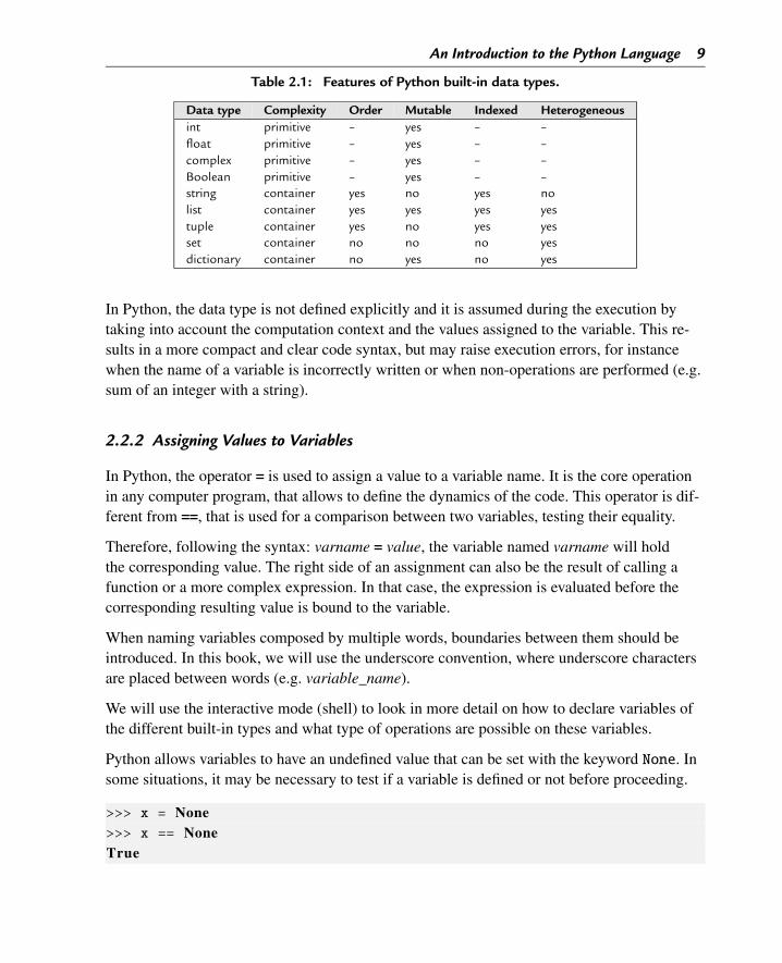
Table 2.1 provides a summary of the different features of Python primitive and container datatypes. The last column indicates if the container type allows different types of their elementsor not.

An Introduction to the Python Language 9

Table 2.1: Features of Python built-in data types.

Data type Complexity Order Mutable Indexed Heterogeneousint primitive – yes – –float primitive – yes – –complex primitive – yes – –Boolean primitive – yes – –string container yes no yes nolist container yes yes yes yestuple container yes no yes yesset container no no no yesdictionary container no yes no yes

In Python, the data type is not defined explicitly and it is assumed during the execution bytaking into account the computation context and the values assigned to the variable. This re-sults in a more compact and clear code syntax, but may raise execution errors, for instancewhen the name of a variable is incorrectly written or when non-operations are performed (e.g.sum of an integer with a string).

2.2.2 Assigning Values to Variables

In Python, the operator = is used to assign a value to a variable name. It is the core operationin any computer program, that allows to define the dynamics of the code. This operator is dif-ferent from ==, that is used for a comparison between two variables, testing their equality.

Therefore, following the syntax: varname = value, the variable named varname will holdthe corresponding value. The right side of an assignment can also be the result of calling afunction or a more complex expression. In that case, the expression is evaluated before thecorresponding resulting value is bound to the variable.

When naming variables composed by multiple words, boundaries between them should beintroduced. In this book, we will use the underscore convention, where underscore charactersare placed between words (e.g. variable_name).

We will use the interactive mode (shell) to look in more detail on how to declare variables ofthe different built-in types and what type of operations are possible on these variables.

Python allows variables to have an undefined value that can be set with the keyword None. Insome situations, it may be necessary to test if a variable is defined or not before proceeding.

>>> x = None>>> x == NoneTrue

10 Chapter 2

If a variable is no longer being used it can be removed by using the del clause.

>>> d e l x

2.2.3 Numerical and Logical Variables

Numeric variables can be either integer, floating point (real numbers), or complex numbers.Boolean variables can have a True or False value and are a particular case of the integertype, corresponding to 1 and 0, respectively.

# integer

>>> sequence_length = 320

# floating

>>> average_score = 23.145

# Boolean

>>> is_sequence = True>>> contains_substring = F a l s e

Multiple variables can also be assigned with the same value in a single line:

>>> a = b = c = 1

Multiple values can be assigned to different variables in a single instruction, in the order theyare declared. In this case, variables and values are separated by commas:

>>> a, b, c = 1, 2, 3

Assignments using expressions in the right hand side are possible. In this case, the evaluationof the expression follows the arithmetic precedence rules.

>>> a = 2∗(1+2)

Variable values can also be swapped in the same line.

>>> a,b,c = c,a,b

The following binary arithmetic operators can be applied to two numeric variables:

• + – sum;• - – difference;• * – multiplication;

An Introduction to the Python Language 11

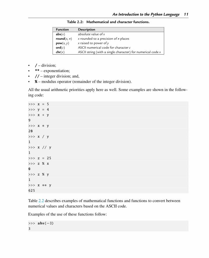
Table 2.2: Mathematical and character functions.

Function Descriptionabs(x) absolute value of xround(x, n) x rounded to a precision of n placespow(x, y) x raised to power of yord(c) ASCII numerical code for character cchr(x) ASCII string (with a single character) for numerical code x

• / – division;• ** – exponentiation;• // – integer division; and,• % – modulus operator (remainder of the integer division).

All the usual arithmetic priorities apply here as well. Some examples are shown in the follow-ing code:

>>> x = 5

>>> y = 4

>>> x + y

9

>>> x ∗ y20

>>> x / y

1

>>> x // y

1

>>> z = 25

>>> z % x

0

>>> z % y

1

>>> x ∗∗ y625

Table 2.2 describes examples of mathematical functions and functions to convert betweennumerical values and characters based on the ASCII code.

Examples of the use of these functions follow:

>>> abs(−3)3

12 Chapter 2

>>> round(3.4)3.0

>>> f l o a t (2)2.0

>>> i n t (3.4)3

>>> i n t (4.6)4

>>> i n t (−2.3)−2>>> 0.00000000000001

1e−14>>> 2.3e−30.0023

>>> chr(97)’a’

>>> ord(’a’)97

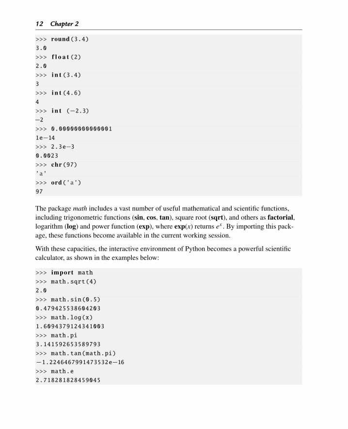
The package math includes a vast number of useful mathematical and scientific functions,including trigonometric functions (sin, cos, tan), square root (sqrt), and others as factorial,logarithm (log) and power function (exp), where exp(x) returns ex . By importing this pack-age, these functions become available in the current working session.

With these capacities, the interactive environment of Python becomes a powerful scientificcalculator, as shown in the examples below:

>>> import math>>> math.sqrt(4)

2.0

>>> math.sin(0.5)

0.479425538604203

>>> math.log(x)

1.6094379124341003

>>> math.pi

3.141592653589793

>>> math.tan(math.pi)

−1.2246467991473532e−16>>> math.e

2.718281828459045

An Introduction to the Python Language 13

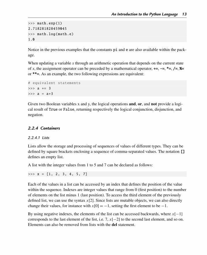
>>> math.exp(1)

2.718281828459045

>>> math.log(math.e)

1.0

Notice in the previous examples that the constants pi and e are also available within the pack-age.

When updating a variable x through an arithmetic operation that depends on the current stateof x, the assignment operator can be preceded by a mathematical operator, +=, -=, *=, /=, %=or **=. As an example, the two following expressions are equivalent:

# equivalent statements

>>> a += 3

>>> a = a+3

Given two Boolean variables x and y, the logical operations and, or, and not provide a logi-cal result of True or False, returning respectively the logical conjunction, disjunction, andnegation.

2.2.4 Containers

2.2.4.1 Lists

Lists allow the storage and processing of sequences of values of different types. They can bedefined by square brackets enclosing a sequence of comma-separated values. The notation []defines an empty list.

A list with the integer values from 1 to 5 and 7 can be declared as follows:

>>> x = [1, 2, 3, 4, 5, 7]

Each of the values in a list can be accessed by an index that defines the position of the valuewithin the sequence. Indexes are integer values that range from 0 (first position) to the numberof elements on the list minus 1 (last position). To access the third element of the previouslydefined list, we can use the syntax x[2]. Since lists are mutable objects, we can also directlychange their values, for instance with x[0] = −1, setting the first element to be −1.

By using negative indexes, the elements of the list can be accessed backwards, where x[−1]corresponds to the last element of the list, i.e. 7, x[−2] to the second last element, and so on.Elements can also be removed from lists with the del statement.

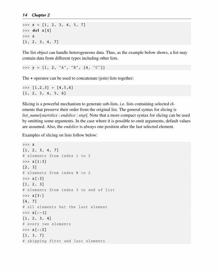
14 Chapter 2

>>> x = [1, 2, 3, 4, 5, 7]

>>> d e l x[4]>>> x

[1, 2, 3, 4, 7]

The list object can handle heterogeneous data. Thus, as the example below shows, a list maycontain data from different types including other lists.

>>> y = [1, 2, "A", "B", [4, "C"]]

The + operator can be used to concatenate (join) lists together:

>>> [1,2,3] + [4,5,6]

[1, 2, 3, 4, 5, 6]

Slicing is a powerful mechanism to generate sub-lists, i.e. lists containing selected el-ements that preserve their order from the original list. The general syntax for slicing islist_name[startslice : endslice : step]. Note that a more compact syntax for slicing can be usedby omitting some arguments. In the case where it is possible to omit arguments, default valuesare assumed. Also, the endslice is always one position after the last selected element.

Examples of slicing on lists follow below:

>>> x

[1, 2, 3, 4, 7]

# elements from index 1 to 2

>>> x[1:3]

[2, 3]

# elements from index 0 to 2

>>> x[:3]

[1, 2, 3]

# elements from index 3 to end of list

>>> x[3:]

[4, 7]

# all elements but the last element

>>> x[:−1][1, 2, 3, 4]

# every two elements

>>> x[::2]

[1, 3, 7]

# skipping first and last elements

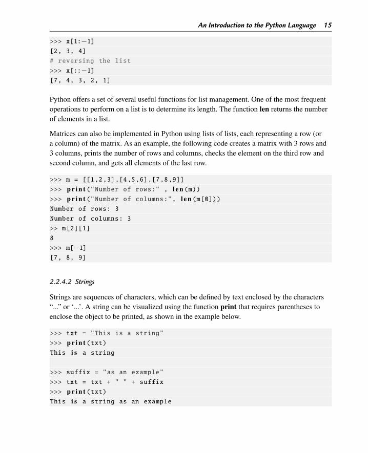
An Introduction to the Python Language 15

>>> x[1:−1][2, 3, 4]

# reversing the list

>>> x[::−1][7, 4, 3, 2, 1]

Python offers a set of several useful functions for list management. One of the most frequentoperations to perform on a list is to determine its length. The function len returns the numberof elements in a list.

Matrices can also be implemented in Python using lists of lists, each representing a row (ora column) of the matrix. As an example, the following code creates a matrix with 3 rows and3 columns, prints the number of rows and columns, checks the element on the third row andsecond column, and gets all elements of the last row.

>>> m = [[1,2,3],[4,5,6],[7,8,9]]

>>> p r i n t ("Number of rows:" , l e n (m))>>> p r i n t ("Number of columns:", l e n (m[0]))Number of rows: 3

Number of columns: 3

>> m[2][1]

8

>>> m[−1][7, 8, 9]

2.2.4.2 Strings

Strings are sequences of characters, which can be defined by text enclosed by the characters“...” or ‘...’. A string can be visualized using the function print that requires parentheses toenclose the object to be printed, as shown in the example below.

>>> txt = "This is a string"

>>> p r i n t (txt)This i s a string

>>> suffix = "as an example"

>>> txt = txt + " " + suffix

>>> p r i n t (txt)This i s a string as an example

16 Chapter 2

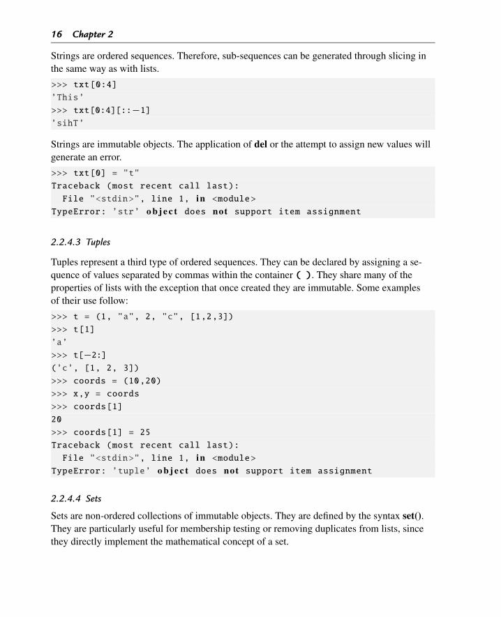
Strings are ordered sequences. Therefore, sub-sequences can be generated through slicing inthe same way as with lists.

>>> txt[0:4]

’This’

>>> txt[0:4][::−1]’sihT’

Strings are immutable objects. The application of del or the attempt to assign new values willgenerate an error.

>>> txt[0] = "t"

Traceback (most recent call last):

File "<stdin>", line 1, in <module>

TypeError: ’str’ o b j e c t does not support item assignment

2.2.4.3 Tuples

Tuples represent a third type of ordered sequences. They can be declared by assigning a se-quence of values separated by commas within the container ( ). They share many of theproperties of lists with the exception that once created they are immutable. Some examplesof their use follow:

>>> t = (1, "a", 2, "c", [1,2,3])

>>> t[1]

’a’

>>> t[−2:](’c’, [1, 2, 3])

>>> coords = (10,20)

>>> x,y = coords

>>> coords[1]

20

>>> coords[1] = 25

Traceback (most recent call last):

File "<stdin>", line 1, in <module>

TypeError: ’tuple’ o b j e c t does not support item assignment

2.2.4.4 Sets

Sets are non-ordered collections of immutable objects. They are defined by the syntax set().They are particularly useful for membership testing or removing duplicates from lists, sincethey directly implement the mathematical concept of a set.

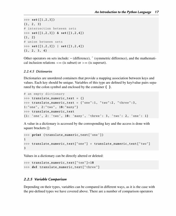
An Introduction to the Python Language 17

>>> s e t ([1,2,3]){1, 2, 3}

# intersection between sets

>>> s e t ([1,2,3]) & s e t ([1,2,4]){1, 2}

# union between sets

>>> s e t ([1,2,3]) | s e t ([1,2,4]){1, 2, 3, 4}

Other operators on sets include: - (difference), ˆ (symmetric difference), and the mathemati-cal inclusion relations <= (is subset) or >= (is superset).

2.2.4.5 Dictionaries

Dictionaries are unordered containers that provide a mapping association between keys andvalues. Each key should be unique. Variables of this type are defined by key/value pairs sepa-rated by the colon symbol and enclosed by the container { }.

# an empty dictionary

>>> translate_numeric_text = {}

>>> translate_numeric_text = {"one":1, "two":2, "three":3,

1:"one", 2:"two", 10:"many"}

>>> translate_numeric_text

{1: ’one’, 2: ’two’, 10: ’many’, ’three’: 3, ’two’: 2, ’one’: 1}

A value in a dictionary is accessed by the corresponding key and the access is done withsquare brackets []:

>>> p r i n t (translate_numeric_text[’one’])1

>>> translate_numeric_text["one"] + translate_numeric_text["two"]

3

Values in a dictionary can be directly altered or deleted:

>>> translate_numeric_text["ten"]=10

>>> d e l translate_numeric_text["three"]

2.2.5 Variable Comparison

Depending on their types, variables can be compared in different ways, as it is the case withthe pre-defined types we have covered above. There are a number of comparison operators

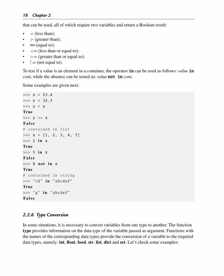
18 Chapter 2

that can be used, all of which require two variables and return a Boolean result:

• < (less than);• > (greater than);• == (equal to);• <= (less than or equal to);• >= (greater than or equal to);• ! = (not equal to).

To test if a value is an element in a container, the operator in can be used as follows: value incont, while the absence can be tested as: value not in cont.

Some examples are given next:

>>> x = 23.4

>>> y = 32.3

>>> y > x

True>>> y <= x

F a l s e# contained in list

>>> x = [1, 2, 3, 4, 7]

>>> 2 in x

True>>> 5 in x

F a l s e>>> 8 not in x

True# contained in string

>>> "cd" in "abcdef"

True>>> "g" in "abcdef"

F a l s e

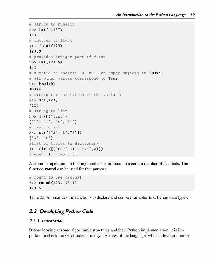
2.2.6 Type Conversion

In some situations, it is necessary to convert variables from one type to another. The functiontype provides information on the data type of the variable passed as argument. Functions withthe names of the corresponding data types provide the conversion of a variable to the requireddata types, namely: int, float, bool, str, list, dict and set. Let’s check some examples:

An Introduction to the Python Language 19

# string to numeric

>>> i n t ("123")123

# integer to float

>>> f l o a t (123)123.0

# provides integer part of float

>>> i n t (123.5)123

# numeric to boolean. 0, null or empty objects to F a l s e .# all other values correspond to True.>>> bool (0)F a l s e# string representation of the variable

>>> s t r (123)’123’

# string to list

>>> l i s t ("list")[’l’, ’i’, ’s’, ’t’]

# list to set

>>> s e t (["A","B","A"]){’A’, ’B’}

#list of tuples to dictionary

>>> d i c t ([("one",1),("two",2)]){’one’: 1, ’two’: 2}

A common operation on floating numbers is to round to a certain number of decimals. Thefunction round can be used for that purpose:

# round to one decimal

>>> round(123.456,1)123.5

Table 2.3 summarizes the functions to declare and convert variables to different data types.

2.3 Developing Python Code

2.3.1 Indentation

Before looking at some algorithmic structures and their Python implementation, it is im-portant to check the set of indentation syntax rules of the language, which allow for a more

20 Chapter 2

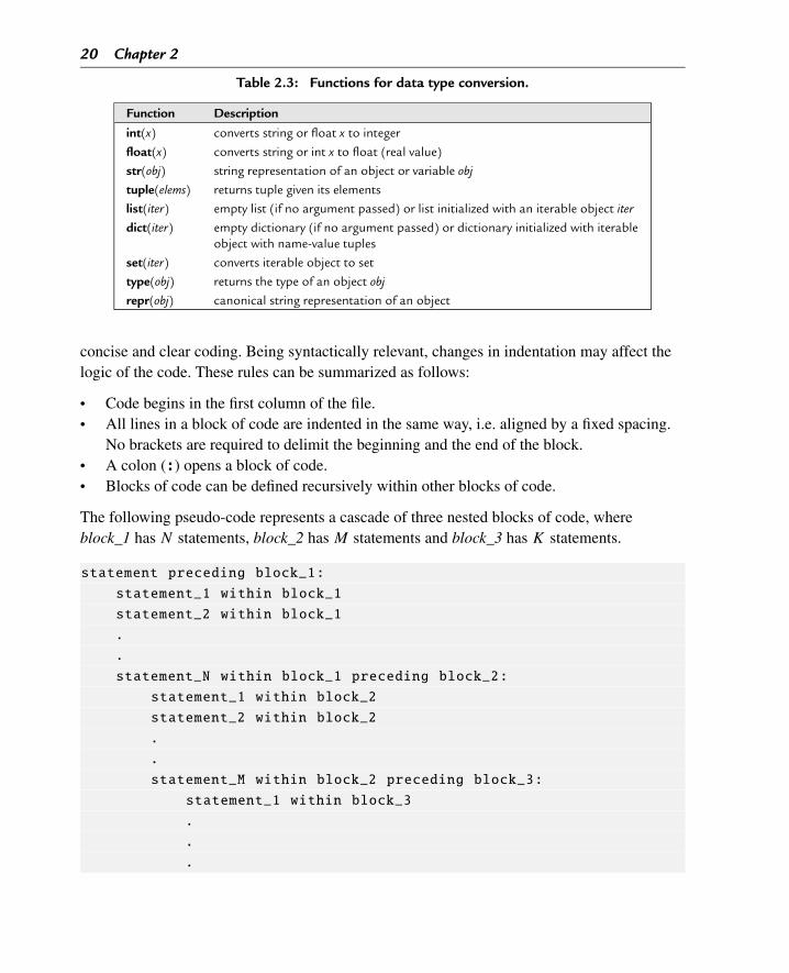
Table 2.3: Functions for data type conversion.

Function Description

int(x) converts string or float x to integer

float(x) converts string or int x to float (real value)

str(obj) string representation of an object or variable obj

tuple(elems) returns tuple given its elements

list(iter) empty list (if no argument passed) or list initialized with an iterable object iter

dict(iter) empty dictionary (if no argument passed) or dictionary initialized with iterableobject with name-value tuples

set(iter) converts iterable object to set

type(obj) returns the type of an object obj

repr(obj) canonical string representation of an object

concise and clear coding. Being syntactically relevant, changes in indentation may affect thelogic of the code. These rules can be summarized as follows:

• Code begins in the first column of the file.• All lines in a block of code are indented in the same way, i.e. aligned by a fixed spacing.

No brackets are required to delimit the beginning and the end of the block.• A colon (:) opens a block of code.• Blocks of code can be defined recursively within other blocks of code.

The following pseudo-code represents a cascade of three nested blocks of code, whereblock_1 has N statements, block_2 has M statements and block_3 has K statements.

statement preceding block_1:

statement_1 within block_1

statement_2 within block_1

.

.

statement_N within block_1 preceding block_2:

statement_1 within block_2

statement_2 within block_2

.

.

statement_M within block_2 preceding block_3:

statement_1 within block_3

.

.

.

An Introduction to the Python Language 21

statement_K within block_3

statement after block_1

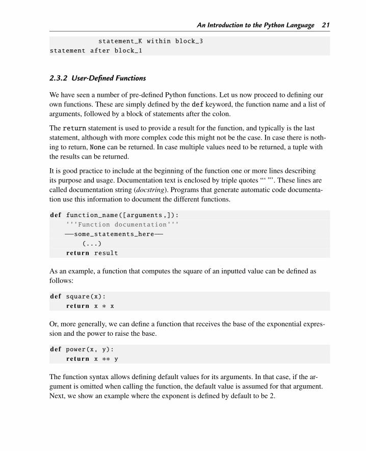
2.3.2 User-Defined Functions

We have seen a number of pre-defined Python functions. Let us now proceed to defining ourown functions. These are simply defined by the def keyword, the function name and a list ofarguments, followed by a block of statements after the colon.

The return statement is used to provide a result for the function, and typically is the laststatement, although with more complex code this might not be the case. In case there is noth-ing to return, None can be returned. In case multiple values need to be returned, a tuple withthe results can be returned.

It is good practice to include at the beginning of the function one or more lines describingits purpose and usage. Documentation text is enclosed by triple quotes “‘ ”’. These lines arecalled documentation string (docstring). Programs that generate automatic code documenta-tion use this information to document the different functions.

def function_name([arguments ,]):’’’Function documentation’’’

−−some_statements_here−−(...)

re turn result

As an example, a function that computes the square of an inputted value can be defined asfollows:

def square(x):re turn x ∗ x

Or, more generally, we can define a function that receives the base of the exponential expres-sion and the power to raise the base.

def power(x, y):re turn x ∗∗ y

The function syntax allows defining default values for its arguments. In that case, if the ar-gument is omitted when calling the function, the default value is assumed for that argument.Next, we show an example where the exponent is defined by default to be 2.

22 Chapter 2

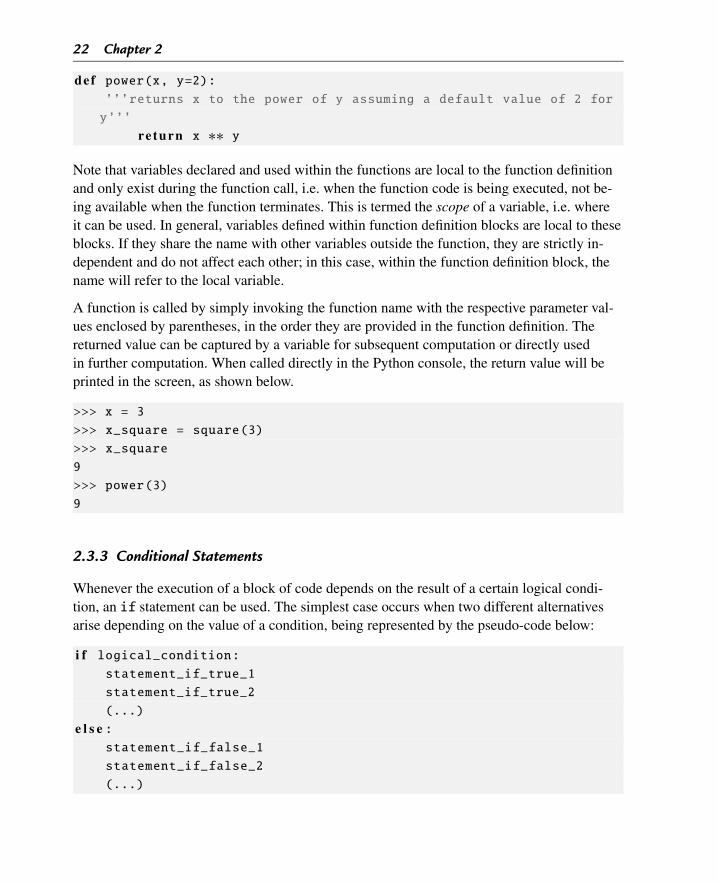
def power(x, y=2):’’’returns x to the power of y assuming a default value of 2 for

y’’’

re turn x ∗∗ y

Note that variables declared and used within the functions are local to the function definitionand only exist during the function call, i.e. when the function code is being executed, not be-ing available when the function terminates. This is termed the scope of a variable, i.e. whereit can be used. In general, variables defined within function definition blocks are local to theseblocks. If they share the name with other variables outside the function, they are strictly in-dependent and do not affect each other; in this case, within the function definition block, thename will refer to the local variable.

A function is called by simply invoking the function name with the respective parameter val-ues enclosed by parentheses, in the order they are provided in the function definition. Thereturned value can be captured by a variable for subsequent computation or directly usedin further computation. When called directly in the Python console, the return value will beprinted in the screen, as shown below.

>>> x = 3

>>> x_square = square(3)

>>> x_square

9

>>> power(3)

9

2.3.3 Conditional Statements

Whenever the execution of a block of code depends on the result of a certain logical condi-tion, an if statement can be used. The simplest case occurs when two different alternativesarise depending on the value of a condition, being represented by the pseudo-code below:

i f logical_condition:statement_if_true_1

statement_if_true_2

(...)

e l s e :statement_if_false_1

statement_if_false_2

(...)

An Introduction to the Python Language 23

In this case, the statements of the first block (below the if) are executed when the conditionis true, while the statements in the second block (below the else) are executed otherwise.Note that the else block may not exist if there are no statements to execute if the condition isfalse.

If there are more than two alternative blocks of code, several elif (with the meaning else if)branches may exist with additional logical conditions, while a single final else clause exists,for the case when all previous conditions fail. The pseudo-code below represents the case withmultiple conditions:

i f logical_condition1:statement_1_condition1

(...)

e l i f logical_condition_2:statement_1_condition2

(...)

( e l i f ...)e l s e :

statement_1_else

(...)

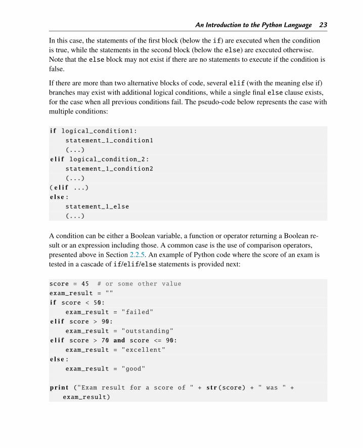
A condition can be either a Boolean variable, a function or operator returning a Boolean re-sult or an expression including those. A common case is the use of comparison operators,presented above in Section 2.2.5. An example of Python code where the score of an exam istested in a cascade of if/elif/else statements is provided next:

score = 45 # or some other value

exam_result = ""

i f score < 50:exam_result = "failed"

e l i f score > 90:exam_result = "outstanding"

e l i f score > 70 and score <= 90:exam_result = "excellent"

e l s e :exam_result = "good"

p r i n t ("Exam result for a score of " + s t r (score) + " was " +exam_result)

24 Chapter 2

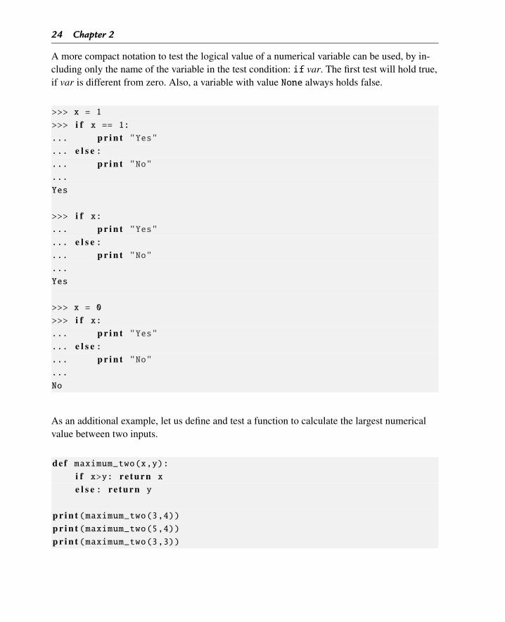
A more compact notation to test the logical value of a numerical variable can be used, by in-cluding only the name of the variable in the test condition: if var. The first test will hold true,if var is different from zero. Also, a variable with value None always holds false.

>>> x = 1

>>> i f x == 1:... p r i n t "Yes"... e l s e :... p r i n t "No"...

Yes

>>> i f x:... p r i n t "Yes"... e l s e :... p r i n t "No"...

Yes

>>> x = 0

>>> i f x:... p r i n t "Yes"... e l s e :... p r i n t "No"...

No

As an additional example, let us define and test a function to calculate the largest numericalvalue between two inputs.

def maximum_two(x,y):i f x>y: re turn xe l s e : re turn y

p r i n t (maximum_two(3,4))p r i n t (maximum_two(5,4))p r i n t (maximum_two(3,3))

An Introduction to the Python Language 25

2.3.4 Conditional Loops

If a statement needs to be executed multiple times (zero or more times) depending on a testcondition holding true, the use of a while statement can be appropriate. The pseudo-code ofthe block of statements within a while cycle is the following:

whi le condition:statement1_inside_while

statement2_inside_while

(...)

next_statement_after_while

In this case, the statements in the block will be executed while the condition holds true. Whenthe condition switches to false, the loop ends, and the program flow follows with the nextstatement. This means that, to avoid infinite cycles, the programmer needs to insure that thecondition will be false at some point in the program execution.

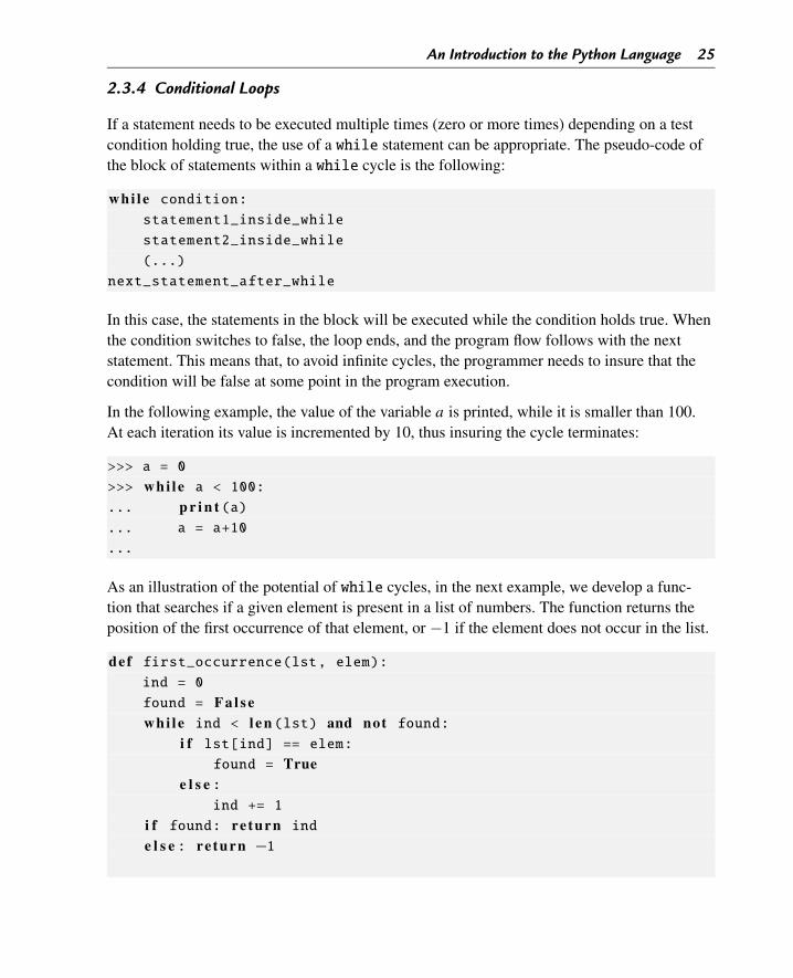
In the following example, the value of the variable a is printed, while it is smaller than 100.At each iteration its value is incremented by 10, thus insuring the cycle terminates:

>>> a = 0

>>> whi le a < 100:... p r i n t (a)... a = a+10

...

As an illustration of the potential of while cycles, in the next example, we develop a func-tion that searches if a given element is present in a list of numbers. The function returns theposition of the first occurrence of that element, or −1 if the element does not occur in the list.

def first_occurrence(lst, elem):ind = 0

found = F a l s ewhi l e ind < l e n (lst) and not found:

i f lst[ind] == elem:found = True

e l s e :ind += 1

i f found: re turn ind

e l s e : re turn −1

26 Chapter 2

l = [1,3,5,7,9]

p r i n t (first_occurrence(l, 5))p r i n t (first_occurrence(l, 2))

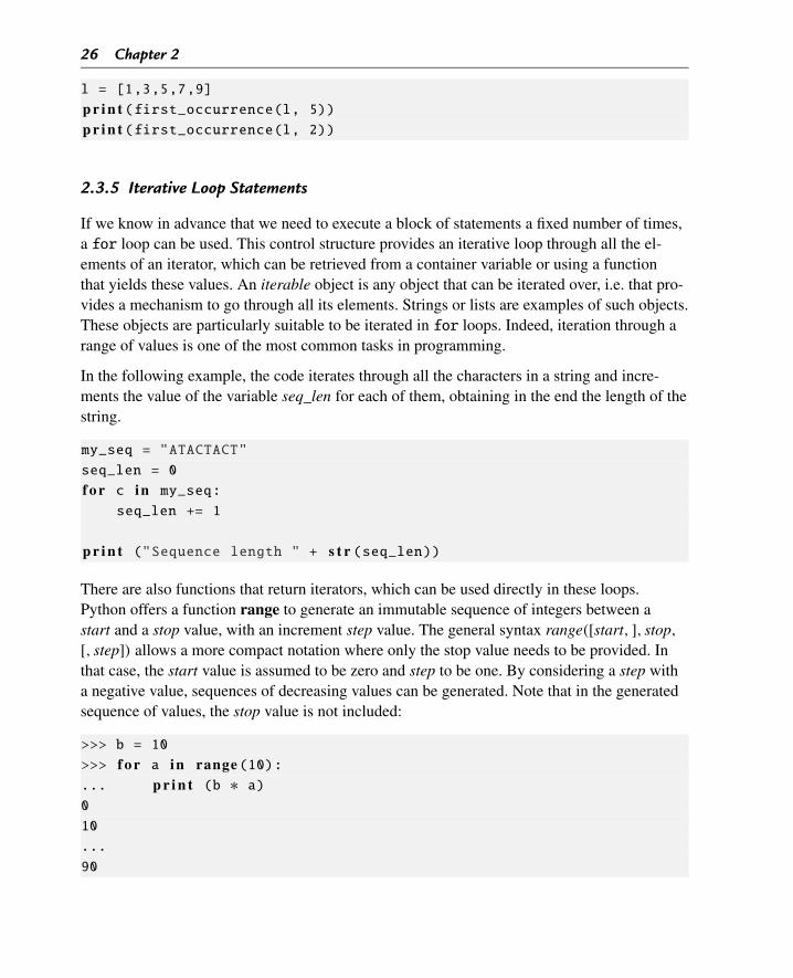
2.3.5 Iterative Loop Statements

If we know in advance that we need to execute a block of statements a fixed number of times,a for loop can be used. This control structure provides an iterative loop through all the el-ements of an iterator, which can be retrieved from a container variable or using a functionthat yields these values. An iterable object is any object that can be iterated over, i.e. that pro-vides a mechanism to go through all its elements. Strings or lists are examples of such objects.These objects are particularly suitable to be iterated in for loops. Indeed, iteration through arange of values is one of the most common tasks in programming.

In the following example, the code iterates through all the characters in a string and incre-ments the value of the variable seq_len for each of them, obtaining in the end the length of thestring.

my_seq = "ATACTACT"

seq_len = 0

f o r c in my_seq:

seq_len += 1

p r i n t ("Sequence length " + s t r (seq_len))

There are also functions that return iterators, which can be used directly in these loops.Python offers a function range to generate an immutable sequence of integers between astart and a stop value, with an increment step value. The general syntax range([start, ], stop,

[, step]) allows a more compact notation where only the stop value needs to be provided. Inthat case, the start value is assumed to be zero and step to be one. By considering a step witha negative value, sequences of decreasing values can be generated. Note that in the generatedsequence of values, the stop value is not included:

>>> b = 10

>>> f o r a in range(10):... p r i n t (b ∗ a)0

10

...

90

An Introduction to the Python Language 27

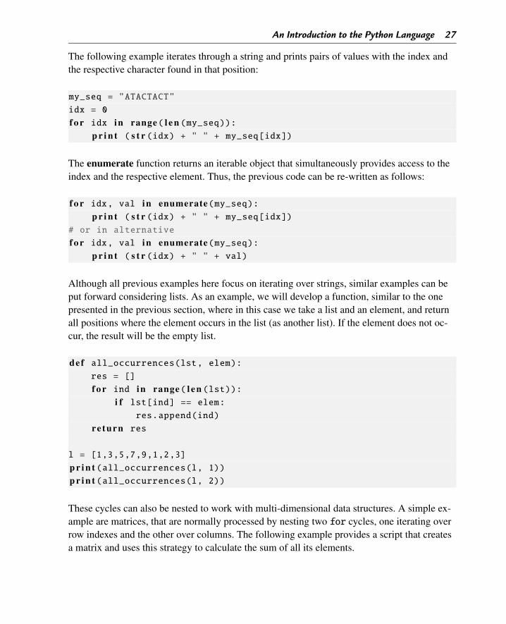
The following example iterates through a string and prints pairs of values with the index andthe respective character found in that position:

my_seq = "ATACTACT"

idx = 0

f o r idx in range( l e n (my_seq)):p r i n t ( s t r (idx) + " " + my_seq[idx])

The enumerate function returns an iterable object that simultaneously provides access to theindex and the respective element. Thus, the previous code can be re-written as follows:

f o r idx, val in enumerate(my_seq):p r i n t ( s t r (idx) + " " + my_seq[idx])

# or in alternative

f o r idx, val in enumerate(my_seq):p r i n t ( s t r (idx) + " " + val)

Although all previous examples here focus on iterating over strings, similar examples can beput forward considering lists. As an example, we will develop a function, similar to the onepresented in the previous section, where in this case we take a list and an element, and returnall positions where the element occurs in the list (as another list). If the element does not oc-cur, the result will be the empty list.

def all_occurrences(lst, elem):res = []

f o r ind in range( l e n (lst)):i f lst[ind] == elem:

res.append(ind)

re turn res

l = [1,3,5,7,9,1,2,3]

p r i n t (all_occurrences(l, 1))p r i n t (all_occurrences(l, 2))

These cycles can also be nested to work with multi-dimensional data structures. A simple ex-ample are matrices, that are normally processed by nesting two for cycles, one iterating overrow indexes and the other over columns. The following example provides a script that createsa matrix and uses this strategy to calculate the sum of all its elements.

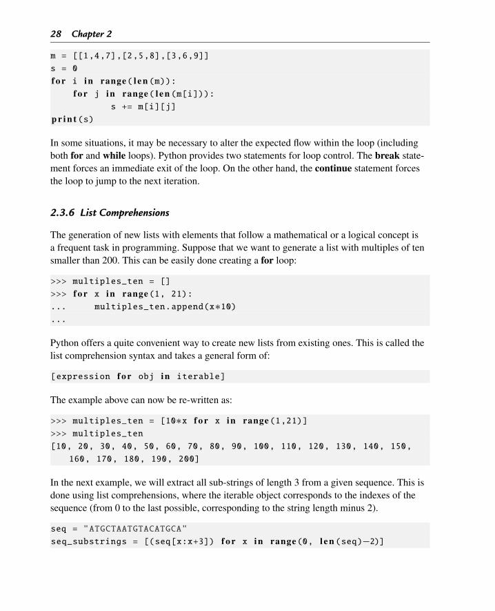
28 Chapter 2

m = [[1,4,7],[2,5,8],[3,6,9]]

s = 0

f o r i in range( l e n (m)):f o r j in range( l e n (m[i])):

s += m[i][j]

p r i n t (s)

In some situations, it may be necessary to alter the expected flow within the loop (includingboth for and while loops). Python provides two statements for loop control. The break state-ment forces an immediate exit of the loop. On the other hand, the continue statement forcesthe loop to jump to the next iteration.

2.3.6 List Comprehensions

The generation of new lists with elements that follow a mathematical or a logical concept isa frequent task in programming. Suppose that we want to generate a list with multiples of tensmaller than 200. This can be easily done creating a for loop:

>>> multiples_ten = []

>>> f o r x in range(1, 21):... multiples_ten.append(x∗10)...

Python offers a quite convenient way to create new lists from existing ones. This is called thelist comprehension syntax and takes a general form of:

[expression f o r obj in iterable]

The example above can now be re-written as:

>>> multiples_ten = [10∗x f o r x in range(1,21)]>>> multiples_ten

[10, 20, 30, 40, 50, 60, 70, 80, 90, 100, 110, 120, 130, 140, 150,

160, 170, 180, 190, 200]

In the next example, we will extract all sub-strings of length 3 from a given sequence. This isdone using list comprehensions, where the iterable object corresponds to the indexes of thesequence (from 0 to the last possible, corresponding to the string length minus 2).

seq = "ATGCTAATGTACATGCA"

seq_substrings = [(seq[x:x+3]) f o r x in range(0, l e n (seq)−2)]

An Introduction to the Python Language 29

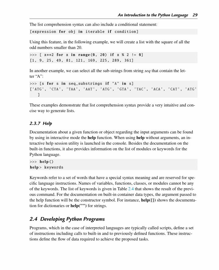
The list comprehension syntax can also include a conditional statement:

[expression f o r obj in iterable i f condition]

Using this feature, in the following example, we will create a list with the square of all theodd numbers smaller than 20.

>>> [ x∗∗2 f o r x in range(0, 20) i f x % 2 != 0][1, 9, 25, 49, 81, 121, 169, 225, 289, 361]

In another example, we can select all the sub-strings from string seq that contain the let-ter “A”:

>>> [s f o r s in seq_substrings i f "A" in s]

[’ATG’, ’CTA’, ’TAA’, ’AAT’, ’ATG’, ’GTA’, ’TAC’, ’ACA’, ’CAT’, ’ATG’

]

These examples demonstrate that list comprehension syntax provide a very intuitive and con-cise way to generate lists.

2.3.7 Help

Documentation about a given function or object regarding the input arguments can be foundby using in interactive mode the help function. When using help without arguments, an in-teractive help session utility is launched in the console. Besides the documentation on thebuilt-in functions, it also provides information on the list of modules or keywords for thePython language.

>>> help ()help > keywords

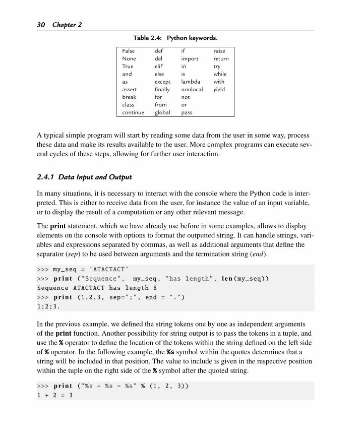
Keywords refer to a set of words that have a special syntax meaning and are reserved for spe-cific language instructions. Names of variables, functions, classes, or modules cannot be anyof the keywords. The list of keywords is given in Table 2.4 that shows the result of the previ-ous command. For the documentation on built-in container data types, the argument passed tothe help function will be the constructor symbol. For instance, help({}) shows the documenta-tion for dictionaries or help("") for strings.

2.4 Developing Python Programs

Programs, which in the case of interpreted languages are typically called scripts, define a setof instructions including calls to built-in and to previously defined functions. These instruc-tions define the flow of data required to achieve the proposed tasks.

30 Chapter 2

Table 2.4: Python keywords.

False def if raiseNone del import returnTrue elif in tryand else is whileas except lambda withassert finally nonlocal yieldbreak for notclass from orcontinue global pass

A typical simple program will start by reading some data from the user in some way, processthese data and make its results available to the user. More complex programs can execute sev-eral cycles of these steps, allowing for further user interaction.

2.4.1 Data Input and Output

In many situations, it is necessary to interact with the console where the Python code is inter-preted. This is either to receive data from the user, for instance the value of an input variable,or to display the result of a computation or any other relevant message.

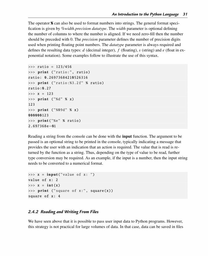
The print statement, which we have already use before in some examples, allows to displayelements on the console with options to format the outputted string. It can handle strings, vari-ables and expressions separated by commas, as well as additional arguments that define theseparator (sep) to be used between arguments and the termination string (end).

>>> my_seq = ’ATACTACT’

>>> p r i n t ("Sequence", my_seq, "has length", l e n (my_seq))Sequence ATACTACT has length 8

>>> p r i n t (1,2,3, sep=";", end = ".")1;2;3.

In the previous example, we defined the string tokens one by one as independent argumentsof the print function. Another possibility for string output is to pass the tokens in a tuple, anduse the % operator to define the location of the tokens within the string defined on the left sideof % operator. In the following example, the %s symbol within the quotes determines that astring will be included in that position. The value to include is given in the respective positionwithin the tuple on the right side of the % symbol after the quoted string.

>>> p r i n t ("%s + %s = %s" % (1, 2, 3))1 + 2 = 3

An Introduction to the Python Language 31

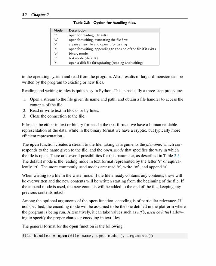
The operator % can also be used to format numbers into strings. The general format speci-fication is given by %width.precision datatype. The width parameter is optional definingthe number of columns to where the number is aligned. If we need zero-fill then the numbershould be preceded with 0. The precision parameter defines the number of precision digitsused when printing floating point numbers. The datatype parameter is always required anddefines the resulting data types: d (decimal integer), f (floating), s (string) and e (float in ex-ponential notation). Some examples follow to illustrate the use of this syntax.

>>> ratio = 123/456

>>> p r i n t ("ratio:", ratio)ratio: 0.26973684210526316

>>> p r i n t ("ratio:%3.2f" % ratio)ratio:0.27

>>> x = 123

>>> p r i n t ("%d" % x)123

>>> p r i n t ("%09d" % x)000000123

>>> p r i n t ("%e" % ratio)2.697368e−01

Reading a string from the console can be done with the input function. The argument to bepassed is an optional string to be printed in the console, typically indicating a message thatprovides the user with an indication that an action is required. The value that is read is re-turned by the function as a string. Thus, depending on the type of value to be read, furthertype conversion may be required. As an example, if the input is a number, then the input stringneeds to be converted to a numerical format.

>>> x = input("value of x: ")value of x: 2

>>> x = i n t (x)>>> p r i n t ("square of x:", square(x))square of x: 4

2.4.2 Reading and Writing From Files

We have seen above that it is possible to pass user input data to Python programs. However,this strategy is not practical for large volumes of data. In that case, data can be saved in files

32 Chapter 2

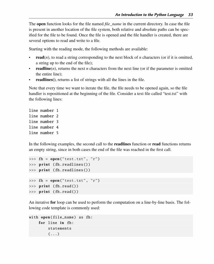
Table 2.5: Option for handling files.

Mode Description’r’ open for reading (default)’w’ open for writing, truncating the file first’x’ create a new file and open it for writing’a’ open for writing, appending to the end of the file if it exists’b’ binary mode’t’ text mode (default)’+’ open a disk file for updating (reading and writing)

in the operating system and read from the program. Also, results of larger dimension can bewritten by the program to existing or new files.

Reading and writing to files is quite easy in Python. This is basically a three-step procedure:

1. Open a stream to the file given its name and path, and obtain a file handler to access thecontents of the file.

2. Read or write text in blocks or by lines.3. Close the connection to the file.

Files can be either in text or binary format. In the text format, we have a human readablerepresentation of the data, while in the binary format we have a cryptic, but typically moreefficient representation.

The open function creates a stream to the file, taking as arguments the filename, which cor-responds to the name given to the file, and the open_mode that specifies the way in whichthe file is open. There are several possibilities for this parameter, as described in Table 2.5.The default mode is the reading mode in text format represented by the letter ‘r’ or equiva-lently ‘rt’. The more commonly used modes are: read ‘r’, write ‘w’, and append ‘a’.

When writing to a file in the write mode, if the file already contains any contents, these willbe overwritten and the new contents will be written starting from the beginning of the file. Ifthe append mode is used, the new contents will be added to the end of the file, keeping anyprevious contents intact.

Among the optional arguments of the open function, encoding is of particular relevance. Ifnot specified, the encoding mode will be assumed to be the one defined in the platform wherethe program is being run. Alternatively, it can take values such as utf 8, ascii or latin1 allow-ing to specify the proper character encoding in text files.

The general format for the open function is the following:

file_handler = open(file_name, open_mode [, arguments])

An Introduction to the Python Language 33

The open function looks for the file named file_name in the current directory. In case the fileis present in another location of the file system, both relative and absolute paths can be spec-ified for the file to be found. Once the file is opened and the file handler is created, there areseveral options to read and write to a file.

Starting with the reading mode, the following methods are available:

• read(n), to read a string corresponding to the next block of n characters (or if it is omitted,a string up to the end of the file);

• readline(n), returns the next n characters from the next line (or if the parameter is omittedthe entire line);

• readlines(), returns a list of strings with all the lines in the file.

Note that every time we want to iterate the file, the file needs to be opened again, so the filehandler is repositioned at the beginning of the file. Consider a text file called “test.txt” withthe following lines:

line number 1

line number 2

line number 3

line number 4

line number 5

In the following examples, the second call to the readlines function or read functions returnsan empty string, since in both cases the end of the file was reached in the first call.

>>> fh = open("test.txt", "r")>>> p r i n t (fh.readlines())>>> p r i n t (fh.readlines())

>>> fh = open("test.txt", "r")>>> p r i n t (fh.read())>>> p r i n t (fh.read())

An iterative for loop can be used to perform the computation on a line-by-line basis. The fol-lowing code template is commonly used:

with open(file_name) as fh:f o r line in fh:

statements

(...)

34 Chapter 2

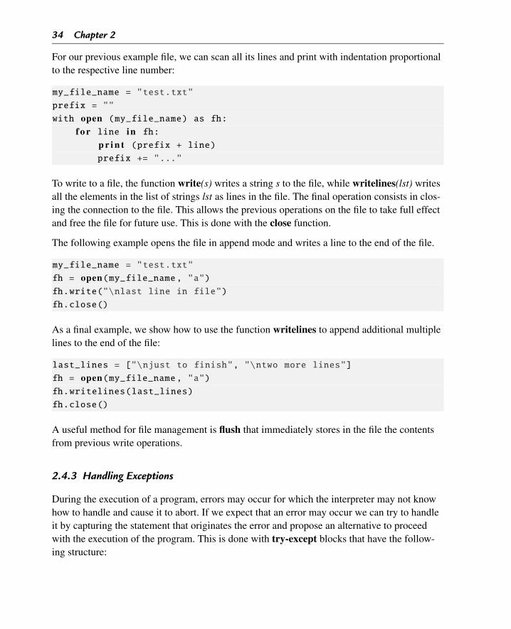
For our previous example file, we can scan all its lines and print with indentation proportionalto the respective line number:

my_file_name = "test.txt"

prefix = ""

with open (my_file_name) as fh:f o r line in fh:

p r i n t (prefix + line)prefix += "..."

To write to a file, the function write(s) writes a string s to the file, while writelines(lst) writesall the elements in the list of strings lst as lines in the file. The final operation consists in clos-ing the connection to the file. This allows the previous operations on the file to take full effectand free the file for future use. This is done with the close function.

The following example opens the file in append mode and writes a line to the end of the file.

my_file_name = "test.txt"

fh = open(my_file_name, "a")fh.write("\nlast line in file")

fh.close()

As a final example, we show how to use the function writelines to append additional multiplelines to the end of the file:

last_lines = ["\njust to finish", "\ntwo more lines"]

fh = open(my_file_name, "a")fh.writelines(last_lines)

fh.close()

A useful method for file management is flush that immediately stores in the file the contentsfrom previous write operations.

2.4.3 Handling Exceptions

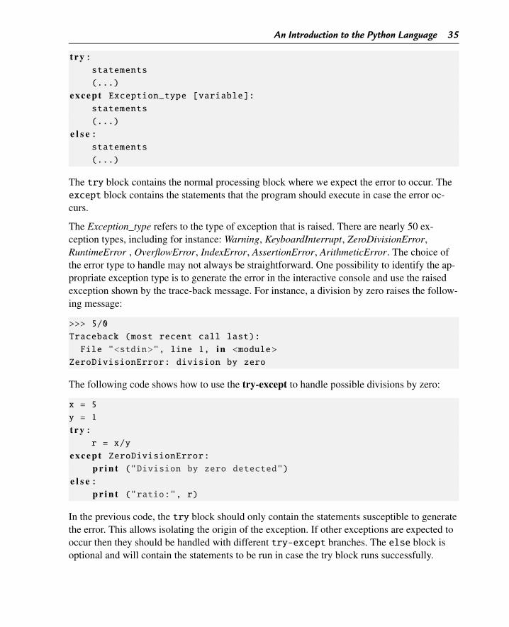
During the execution of a program, errors may occur for which the interpreter may not knowhow to handle and cause it to abort. If we expect that an error may occur we can try to handleit by capturing the statement that originates the error and propose an alternative to proceedwith the execution of the program. This is done with try-except blocks that have the follow-ing structure:

An Introduction to the Python Language 35

t r y :statements

(...)

e x c e p t Exception_type [variable]:statements

(...)

e l s e :statements

(...)

The try block contains the normal processing block where we expect the error to occur. Theexcept block contains the statements that the program should execute in case the error oc-curs.

The Exception_type refers to the type of exception that is raised. There are nearly 50 ex-ception types, including for instance: Warning, KeyboardInterrupt, ZeroDivisionError,RuntimeError , OverflowError, IndexError, AssertionError, ArithmeticError. The choice ofthe error type to handle may not always be straightforward. One possibility to identify the ap-propriate exception type is to generate the error in the interactive console and use the raisedexception shown by the trace-back message. For instance, a division by zero raises the follow-ing message:

>>> 5/0

Traceback (most recent call last):

File "<stdin>", line 1, in <module>

ZeroDivisionError: division by zero

The following code shows how to use the try-except to handle possible divisions by zero:

x = 5

y = 1

t r y :r = x/y

e x c e p t ZeroDivisionError:p r i n t ("Division by zero detected")

e l s e :p r i n t ("ratio:", r)

In the previous code, the try block should only contain the statements susceptible to generatethe error. This allows isolating the origin of the exception. If other exceptions are expected tooccur then they should be handled with different try-except branches. The else block isoptional and will contain the statements to be run in case the try block runs successfully.

36 Chapter 2

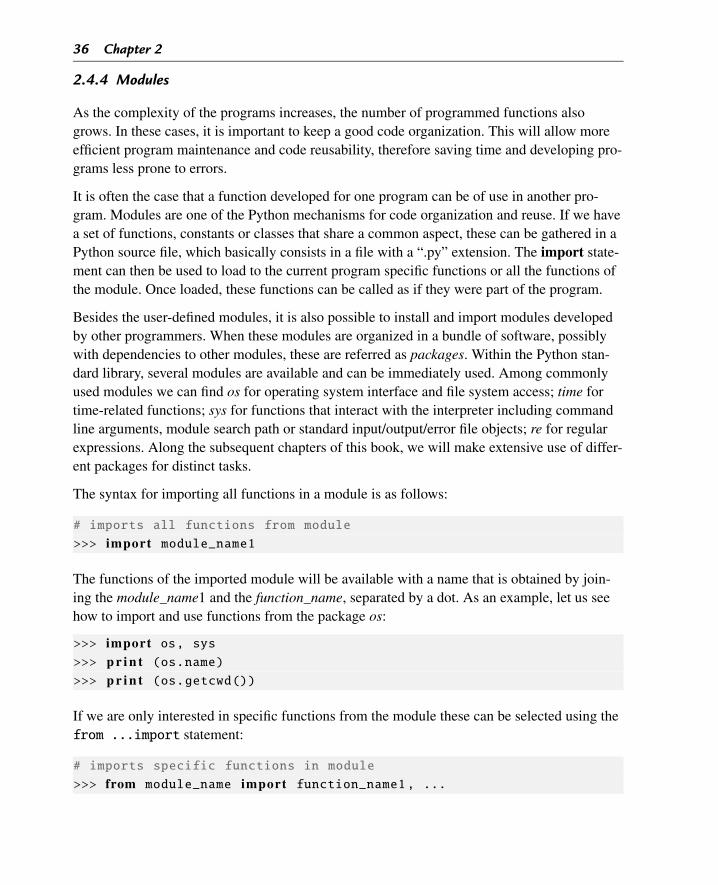
2.4.4 Modules

As the complexity of the programs increases, the number of programmed functions alsogrows. In these cases, it is important to keep a good code organization. This will allow moreefficient program maintenance and code reusability, therefore saving time and developing pro-grams less prone to errors.

It is often the case that a function developed for one program can be of use in another pro-gram. Modules are one of the Python mechanisms for code organization and reuse. If we havea set of functions, constants or classes that share a common aspect, these can be gathered in aPython source file, which basically consists in a file with a “.py” extension. The import state-ment can then be used to load to the current program specific functions or all the functions ofthe module. Once loaded, these functions can be called as if they were part of the program.

Besides the user-defined modules, it is also possible to install and import modules developedby other programmers. When these modules are organized in a bundle of software, possiblywith dependencies to other modules, these are referred as packages. Within the Python stan-dard library, several modules are available and can be immediately used. Among commonlyused modules we can find os for operating system interface and file system access; time fortime-related functions; sys for functions that interact with the interpreter including commandline arguments, module search path or standard input/output/error file objects; re for regularexpressions. Along the subsequent chapters of this book, we will make extensive use of differ-ent packages for distinct tasks.

The syntax for importing all functions in a module is as follows:

# imports all functions from module

>>> import module_name1

The functions of the imported module will be available with a name that is obtained by join-ing the module_name1 and the function_name, separated by a dot. As an example, let us seehow to import and use functions from the package os:

>>> import os, sys>>> p r i n t (os.name)>>> p r i n t (os.getcwd())

If we are only interested in specific functions from the module these can be selected using thefrom ...import statement:

# imports specific functions in module

>>> from module_name import function_name1 , ...

An Introduction to the Python Language 37

Table 2.6: Methods on module math.

Function Description

e, pi, tau, inf, nan mathematical constants and symbols

cos(x), sin(x), tan(x), acos(x), acosh(x),asin(x), asinh(x), atan(x), atanh(x)

different trigonometric functions

sqrt(x) returns the square root of x

pow(x,y) returns x to the power of y

exp(x) returns e raised to the power of x

log2(x), log10(x), log(x, [base]) returns the logarithm of x in different bases

ceil(x) returns the smallest integer greater than or equal to x

factorial(x) returns factorial of x

floor(x) returns the integer part of x

hypot(x,y) returns the Euclidean distance between x and y

degrees(x) convert angle x from radians to degree

radians(x) convert angle x from degrees to radians

In this last case, if the * symbol is placed after the import keyword, all functions of the mod-ule will be imported. It is important to note that in this case, the functions are called only bytheir names without the module name. While this is more readable, it can bring problems iftwo functions have the same name in different modules, so this option should only be usedwith care when this problem can be avoided.

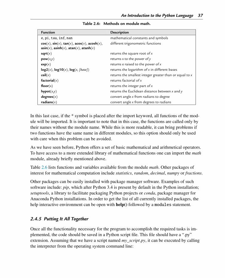
As we have seen before, Python offers a set of basic mathematical and arithmetical operators.To have access to a more extended library of mathematical functions one can import the mathmodule, already briefly mentioned above.

Table 2.6 lists functions and variables available from the module math. Other packages ofinterest for mathematical computation include statistics, random, decimal, numpy or fractions.

Other packages can be easily installed with package manager software. Examples of suchsoftware include: pip, which after Python 3.4 is present by default in the Python installation;setuptools, a library to facilitate packaging Python projects or conda, package manager forAnaconda Python installations. In order to get the list of all currently installed packages, thehelp interactive environment can be open with help() followed by a modules statement.

2.4.5 Putting It All Together

Once all the functionality necessary for the program to accomplish the required tasks is im-plemented, the code should be saved in a Python script file. This file should have a “.py”extension. Assuming that we have a script named my_script.py, it can be executed by callingthe interpreter from the operating system command line:

38 Chapter 2

> python my_script.py

Alternatively, under Unix based operating systems, including Mac OSX, the first line in ourscript can be used to indicate the path to the Python interpreter. This should appear after thesymbols #!, as in #!/path_in_my_os/bin/python, where path_in_my_os is the path to thebinaries folder that contains the Python interpreter. In this case, the program can be calleddirectly without invoking the interpreter:

> my_script.py

Also, if using a proper IDE, there are options to write the script, save it and run it. In manycases, the program will run and show its results within a panel included in the IDE’s interface.

Whenever a Python script is run, the code from the imported modules is interpreted and exe-cuted. In order to prevent immediate execution of the imported code within a module, a con-ditional statement can be used. When a file is run, the special variable _ _name_ _ is set to“_ _main_ _”. With the code below, when the module is run directly, the function main() iscalled and the respective code executed. When, on the other hand, the module is imported bysome other program, the execution of the module’s code is prevented. This feature is particu-larly useful for testing purposes.

i f __name__ == "__main__":main()

With the elements presented in this section, you should be able to start tackling your program-ming challenges and write our own Python programs. To provide an example, let us checka simple program that reads a string, representing a DNA sequence, and computes the fre-quency of each nucleotide, also checking if there are non-valid characters.

def count_bases (seq):dic = {}

seqC = seq.upper()

errors = 0

f o r b in seqC:

i f b in "ACGT":

i f b in dic: dic[b] += 1

e l s e : dic[b] = 1e l s e : errors += 1

re turn dic, errors

def print_perc_dic (dic):

An Introduction to the Python Language 39

sum_values = sum(dic.values())f o r k in s o r t e d (dic.keys()):

p r i n t (" %s −>" % k, " %3.2f" % (dic[k]∗100.0/sum_values), "%")

## main program

seq = input("Input DNA sequence: ")freqs, errors = count_bases(seq)

i f errors > 0:p r i n t ("Sequence is invalid with ", errors , "invalid characters")

e l s e : p r i n t ("Sequence is valid")p r i n t ("Frequencies of the valid characters:")print_perc_dic (freqs)

Notice that the whole code can be put in a single file, or in alternative, the two functions canbe part of a module (let’s say called sequences.py) and in this case, the main program wouldstart with the line:

from sequences import count_bases , printPercDic

2.5 Object-Oriented Programming

2.5.1 Defining Classes and Creating Objects

Object-oriented programming (OOP) is a popular paradigm that is based in the concepts ofobjects, classes and inheritance. This paradigm provides increased modularity, allowing thedeveloped code to be encapsulated and more easily reused. Python supports OOP, allowingthe definition of new classes by the programmer. Also, it provides a number of pre-definedclasses, some of which were already presented in previous sections, including lists and dictio-naries.

Classes are central concepts in OOP, representing an entity to be modeled. Classes allow tomodel objects that represent entities within the programs. They can be used to model en-tities such as strings, biological sequences, or more complex entities such as databases ornetworks.

Classes enclose two major components: one that specifies the data contents to be handled anda second component that specifies the behavior, i.e. the functionality that allows manipulating

40 Chapter 2

the respective contents. In the object-oriented terminology these functions are called meth-ods, while information reflecting the state of the object is stored in variables that are calledattributes.

As a convention for class naming, we will use CamelCase where each letter of a word in classname is represented in uppercase. Attributes are written in lowercase with underscores as forvariable names.

Classes can be created with the instruction class according to the following syntax:

c l a s s ClassName:""" Optional documentation """

−−body_of_the_class−−

In the body of the class, methods are defined, while attributes are used and defined implicitly.For each newly created class, we will need to define a constructor method called _ _init_ _(note the double underscores as prefix and suffix). This method is automatically invoked whennew objects of this class are declared and defines the initial state of the objects that are in-stances of this class.

As an example, the following code implements a very simple class to represent and processbiological sequences. This class contains two attributes seq and seq_type, which represent, re-spectively, a sequence and its biological type (protein, DNA, RNA). The constructor receivesas input the sequence (a string) and assumes “DNA” as the default type, although in the con-structor it can also be set to a different value (“RNA” or “protein”):

c l a s s MySeq:"""Biological sequence class"""

def __init__( s e l f , seq, seq_type = "DNA"):s e l f .seq = seqs e l f .seq_type = seq_type

def print_sequence( s e l f ):p r i n t ("Sequence: " + s e l f .seq)

def get_seq_biotype ( s e l f ):re turn s e l f .seq_type

def show_info_seq ( s e l f ):

An Introduction to the Python Language 41

p r i n t ("Sequence: " + s e l f .seq + " biotype: " + s e l f .seq_type)

def count_occurrences( s e l f , seq_search):re turn s e l f .seq.count(seq_search)

In the methods of the class, self always appears as the first argument. It refers to the newlycreated object instance in the constructor, or to the object over which the method is beingcalled in the other methods. As you can see from Table 2.4, self is not a reserved keywordbut a strong convention of the language.

While a class defines a template, an object is an instance of a class, i.e. a variable that followsthe rules defined by the class. Objects of the same class have the same set of attributes, whilethe specific values for those may be different, and implement the same set of methods. Objectinstantiation, i.e. creating new objects/variables of a class, has the following syntax structure:

object_var = ClassName(arguments)

Also, methods defined within a class can be invoked with the following syntax:

object_var.method_name(arguments)

If a class is defined as above, we can easily create an object instance from that class, accessthe values of its attributes and invoke the defined methods using the following statements (ei-ther on the console or within a script in the same file of the class definition):

s1 = MySeq("ATAATGATAGATAGATGAT")

# access attribute values

p r i n t (s1.seq)p r i n t (s1.seq_type)# calling methods

s1.print_sequence()

p r i n t (s1.get_seq_biotype())

In Python, the attributes of a class can be directly modified. The programmer should evaluateif an attribute should be directly modified or if this modification should be validated before itoccurs and, therefore, be made through a method.

In the next code snippet, an example is shown of a syntactically valid attribute modification,but that is semantically incorrect and would not be desirable. In alternative, a new methodcalled set_seq_biotype is defined to update the attribute, where the validity of the modificationis evaluated before it takes place.

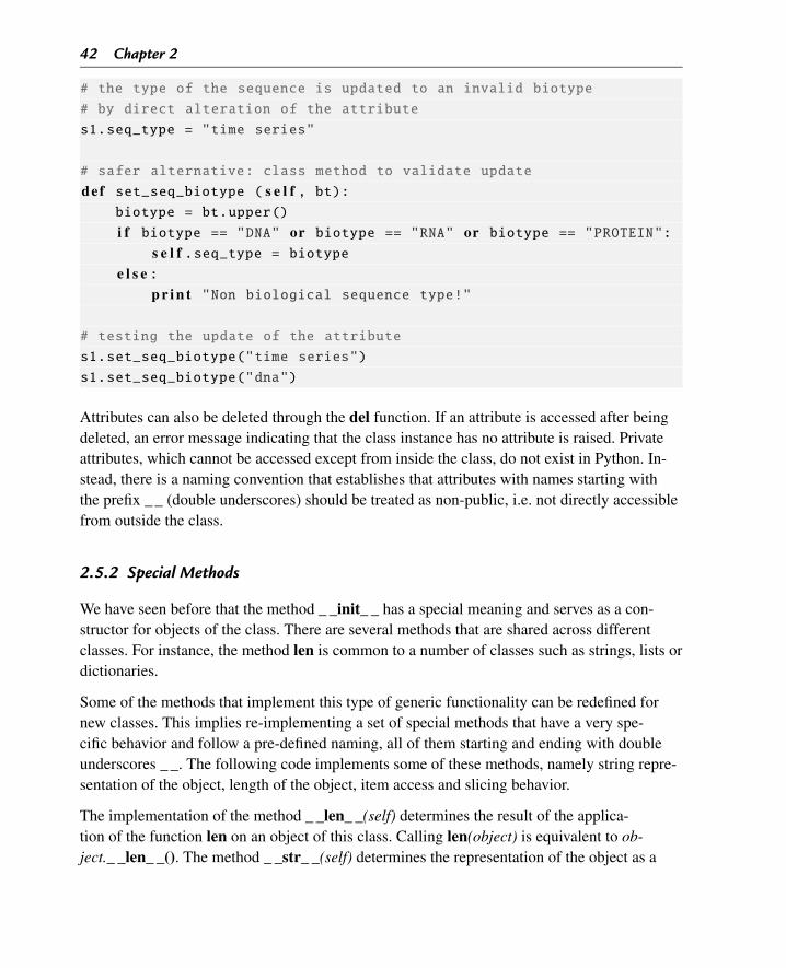
42 Chapter 2

# the type of the sequence is updated to an invalid biotype

# by direct alteration of the attribute

s1.seq_type = "time series"

# safer alternative: class method to validate update

def set_seq_biotype ( s e l f , bt):biotype = bt.upper()

i f biotype == "DNA" or biotype == "RNA" or biotype == "PROTEIN":s e l f .seq_type = biotype

e l s e :p r i n t "Non biological sequence type!"

# testing the update of the attribute

s1.set_seq_biotype("time series")

s1.set_seq_biotype("dna")

Attributes can also be deleted through the del function. If an attribute is accessed after beingdeleted, an error message indicating that the class instance has no attribute is raised. Privateattributes, which cannot be accessed except from inside the class, do not exist in Python. In-stead, there is a naming convention that establishes that attributes with names starting withthe prefix _ _ (double underscores) should be treated as non-public, i.e. not directly accessiblefrom outside the class.

2.5.2 Special Methods

We have seen before that the method _ _init_ _ has a special meaning and serves as a con-structor for objects of the class. There are several methods that are shared across differentclasses. For instance, the method len is common to a number of classes such as strings, lists ordictionaries.

Some of the methods that implement this type of generic functionality can be redefined fornew classes. This implies re-implementing a set of special methods that have a very spe-cific behavior and follow a pre-defined naming, all of them starting and ending with doubleunderscores _ _. The following code implements some of these methods, namely string repre-sentation of the object, length of the object, item access and slicing behavior.

The implementation of the method _ _len_ _(self) determines the result of the applica-tion of the function len on an object of this class. Calling len(object) is equivalent to ob-ject._ _len_ _(). The method _ _str_ _(self) determines the representation of the object as a

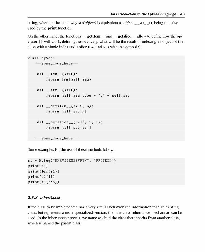
An Introduction to the Python Language 43

string, where in the same way str(object) is equivalent to object._ _str_ _(), being this alsoused by the print function.

On the other hand, the functions _ _getitem_ _ and _ _getslice_ _ allow to define how the op-erator [] will work, defining, respectively, what will be the result of indexing an object of theclass with a single index and a slice (two indexes with the symbol :).

c l a s s MySeq:−−some_code_here−−

def __len__( s e l f ):re turn l e n ( s e l f .seq)

def __str__( s e l f ):re turn s e l f .seq_type + ":" + s e l f .seq

def __getitem__( s e l f , n):re turn s e l f .seq[n]

def __getslice__( s e l f , i, j):re turn s e l f .seq[i:j]

−−some_code_here−−

Some examples for the use of these methods follow:

s1 = MySeq("MKKVSJEMSSVPYW", "PROTEIN")

p r i n t (s1)p r i n t ( l e n (s1))p r i n t (s1[4])p r i n t (s1[2:5])

2.5.3 Inheritance

If the class to be implemented has a very similar behavior and information than an existingclass, but represents a more specialized version, then the class inheritance mechanism can beused. In the inheritance process, we name as child the class that inherits from another class,which is named the parent class.

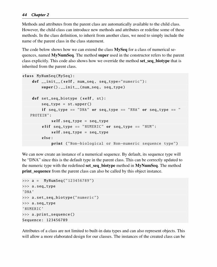
44 Chapter 2

Methods and attributes from the parent class are automatically available to the child class.However, the child class can introduce new methods and attributes or redefine some of thesemethods. In the class definition, to inherit from another class, we need to simply include thename of the parent class in the class statement.

The code below shows how we can extend the class MySeq for a class of numerical se-quences, named MyNumSeq. The method super used in the constructor refers to the parentclass explicitly. This code also shows how we override the method set_seq_biotype that isinherited from the parent class.

c l a s s MyNumSeq(MySeq):def __init__( s e l f , num_seq, seq_type="numeric"):

super().__init__(num_seq, seq_type)

def set_seq_biotype ( s e l f , st):seq_type = st.upper()

i f seq_type == "DNA" or seq_type == "RNA" or seq_type == "PROTEIN":

s e l f .seq_type = seq_typee l i f seq_type == "NUMERIC" or seq_type == "NUM":

s e l f .seq_type = seq_typee l s e :

p r i n t ("Non−biological or Non−numeric sequence type")

We can now create an instance of a numerical sequence. By default, its sequence type willbe “DNA” since this is the default type in the parent class. This can be correctly updated tothe numeric type with the redefined set_seq_biotype method in MyNumSeq. The methodprint_sequence from the parent class can also be called by this object instance.

>>> a = MyNumSeq("123456789")

>>> a.seq_type

’DNA’

>>> a.set_seq_biotype("numeric")

>>> a.seq_type

’NUMERIC’

>>> a.print_sequence()

Sequence: 123456789

Attributes of a class are not limited to built-in data types and can also represent objects. Thiswill allow a more elaborated design for our classes. The instances of the created class can be

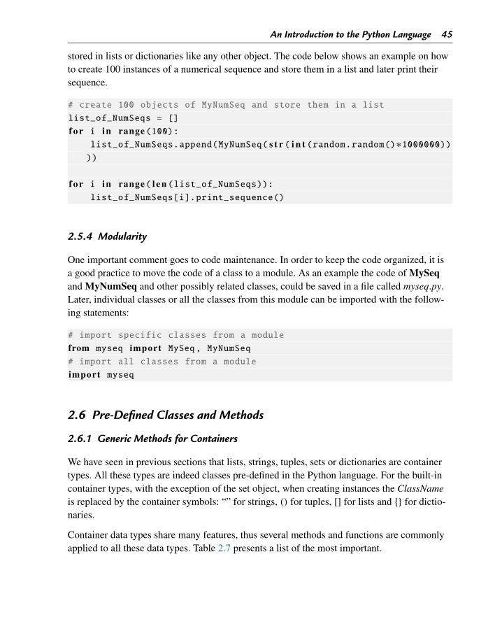
An Introduction to the Python Language 45

stored in lists or dictionaries like any other object. The code below shows an example on howto create 100 instances of a numerical sequence and store them in a list and later print theirsequence.

# create 100 objects of MyNumSeq and store them in a list

list_of_NumSeqs = []

f o r i in range(100):list_of_NumSeqs.append(MyNumSeq( s t r ( i n t (random.random()∗1000000))))

f o r i in range( l e n (list_of_NumSeqs)):list_of_NumSeqs[i].print_sequence()

2.5.4 Modularity

One important comment goes to code maintenance. In order to keep the code organized, it isa good practice to move the code of a class to a module. As an example the code of MySeqand MyNumSeq and other possibly related classes, could be saved in a file called myseq.py.Later, individual classes or all the classes from this module can be imported with the follow-ing statements:

# import specific classes from a module

from myseq import MySeq, MyNumSeq# import all classes from a module

import myseq

2.6 Pre-Defined Classes and Methods

2.6.1 Generic Methods for Containers

We have seen in previous sections that lists, strings, tuples, sets or dictionaries are containertypes. All these types are indeed classes pre-defined in the Python language. For the built-incontainer types, with the exception of the set object, when creating instances the ClassNameis replaced by the container symbols: “” for strings, () for tuples, [] for lists and {} for dictio-naries.

Container data types share many features, thus several methods and functions are commonlyapplied to all these data types. Table 2.7 presents a list of the most important.

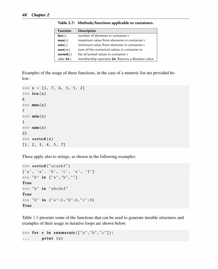
46 Chapter 2

Table 2.7: Methods/functions applicable to containers.

Function Descriptionlen(c) number of elements in container cmax(c) maximum value from elements in container cmin(c) minimum value from elements in container csum(nc) sum of the numerical values in container ncsorted(c) list of sorted values in container cvalue in c membership operator in. Returns a Boolean value

Examples of the usage of these functions, in the case of a numeric list are provided be-low:

>>> x = [1, 7, 4, 3, 5, 2]

>>> l e n (x)6

>>> max(x)7

>>> min(x)1

>>> sum(x)22

>>> s o r t e d (x)[1, 2, 3, 4, 5, 7]

These apply also to strings, as shown in the following examples:

>>> s o r t e d ("acaebf")[’a’, ’a’, ’b’, ’c’, ’e’, ’f’]

>>> "b" in ["a","b",""]

True>>> "b" in "abcdef"

True>>> "b" in {"a":1,"b":2,"c":3}

True

Table 2.8 presents some of the functions that can be used to generate iterable structures andexamples of their usage in iterative loops are shown below.

>>> f o r e in enumerate(["a","b","c"]):... p r i n t (e)

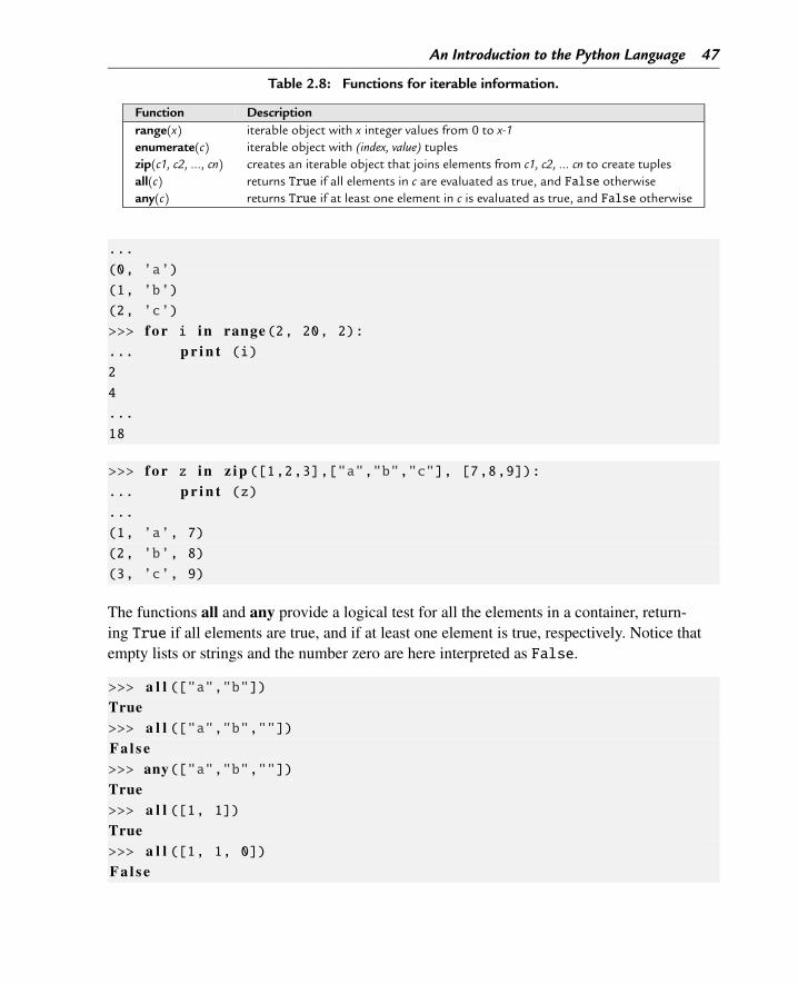
An Introduction to the Python Language 47

Table 2.8: Functions for iterable information.

Function Descriptionrange(x) iterable object with x integer values from 0 to x-1enumerate(c) iterable object with (index, value) tupleszip(c1, c2, ..., cn) creates an iterable object that joins elements from c1, c2, ... cn to create tuplesall(c) returns True if all elements in c are evaluated as true, and False otherwiseany(c) returns True if at least one element in c is evaluated as true, and False otherwise

...

(0, ’a’)

(1, ’b’)

(2, ’c’)

>>> f o r i in range(2, 20, 2):... p r i n t (i)2

4

...

18

>>> f o r z in z i p ([1,2,3],["a","b","c"], [7,8,9]):... p r i n t (z)...

(1, ’a’, 7)

(2, ’b’, 8)

(3, ’c’, 9)

The functions all and any provide a logical test for all the elements in a container, return-ing True if all elements are true, and if at least one element is true, respectively. Notice thatempty lists or strings and the number zero are here interpreted as False.

>>> a l l (["a","b"])True>>> a l l (["a","b",""])F a l s e>>> any(["a","b",""])True>>> a l l ([1, 1])True>>> a l l ([1, 1, 0])F a l s e

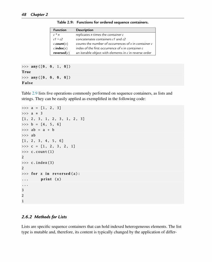
48 Chapter 2

Table 2.9: Functions for ordered sequence containers.

Function Descriptionc * n replicates n times the container cc1 + c2 concatenates containers c1 and c2c.count(x) counts the number of occurrences of x in container cc.index(x) index of the first occurrence of x in container creversed(c) an iterable object with elements in c in reverse order

>>> any([0, 0, 1, 0])True>>> any([0, 0, 0, 0])F a l s e

Table 2.9 lists five operations commonly performed on sequence containers, as lists andstrings. They can be easily applied as exemplified in the following code:

>>> a = [1, 2, 3]

>>> a ∗ 3[1, 2, 3, 1, 2, 3, 1, 2, 3]

>>> b = [4, 5, 6]

>>> ab = a + b

>>> ab

[1, 2, 3, 4, 5, 6]

>>> c = [1, 2, 3, 2, 1]

>>> c.count(1)

2

>>> c.index(3)

2

>>> f o r x i n r e v e r s e d (a):... p r i n t (x)...

3

2

1

2.6.2 Methods for Lists

Lists are specific sequence containers that can hold indexed heterogeneous elements. The listtype is mutable and, therefore, its content is typically changed by the application of differ-

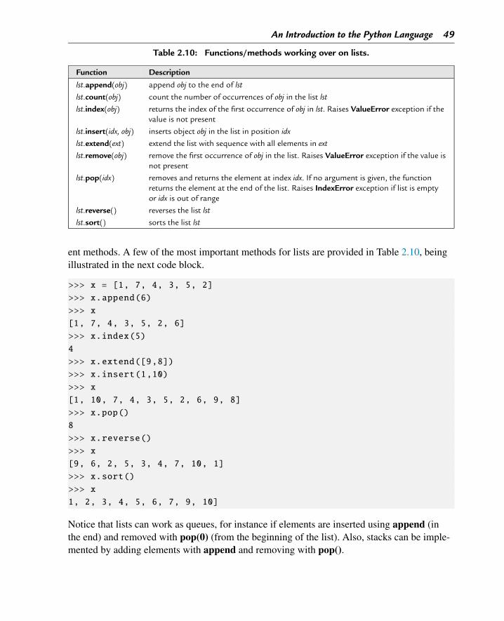
An Introduction to the Python Language 49

Table 2.10: Functions/methods working over on lists.

Function Description

lst.append(obj) append obj to the end of lst

lst.count(obj) count the number of occurrences of obj in the list lst

lst.index(obj) returns the index of the first occurrence of obj in lst. Raises ValueError exception if thevalue is not present

lst.insert(idx, obj) inserts object obj in the list in position idx

lst.extend(ext) extend the list with sequence with all elements in ext

lst.remove(obj) remove the first occurrence of obj in the list. Raises ValueError exception if the value isnot present

lst.pop(idx) removes and returns the element at index idx. If no argument is given, the functionreturns the element at the end of the list. Raises IndexError exception if list is emptyor idx is out of range

lst.reverse() reverses the list lst

lst.sort() sorts the list lst

ent methods. A few of the most important methods for lists are provided in Table 2.10, beingillustrated in the next code block.

>>> x = [1, 7, 4, 3, 5, 2]

>>> x.append(6)

>>> x

[1, 7, 4, 3, 5, 2, 6]

>>> x.index(5)

4

>>> x.extend([9,8])

>>> x.insert(1,10)

>>> x

[1, 10, 7, 4, 3, 5, 2, 6, 9, 8]

>>> x.pop()

8

>>> x.reverse()

>>> x

[9, 6, 2, 5, 3, 4, 7, 10, 1]

>>> x.sort()

>>> x

1, 2, 3, 4, 5, 6, 7, 9, 10]

Notice that lists can work as queues, for instance if elements are inserted using append (inthe end) and removed with pop(0) (from the beginning of the list). Also, stacks can be imple-mented by adding elements with append and removing with pop().

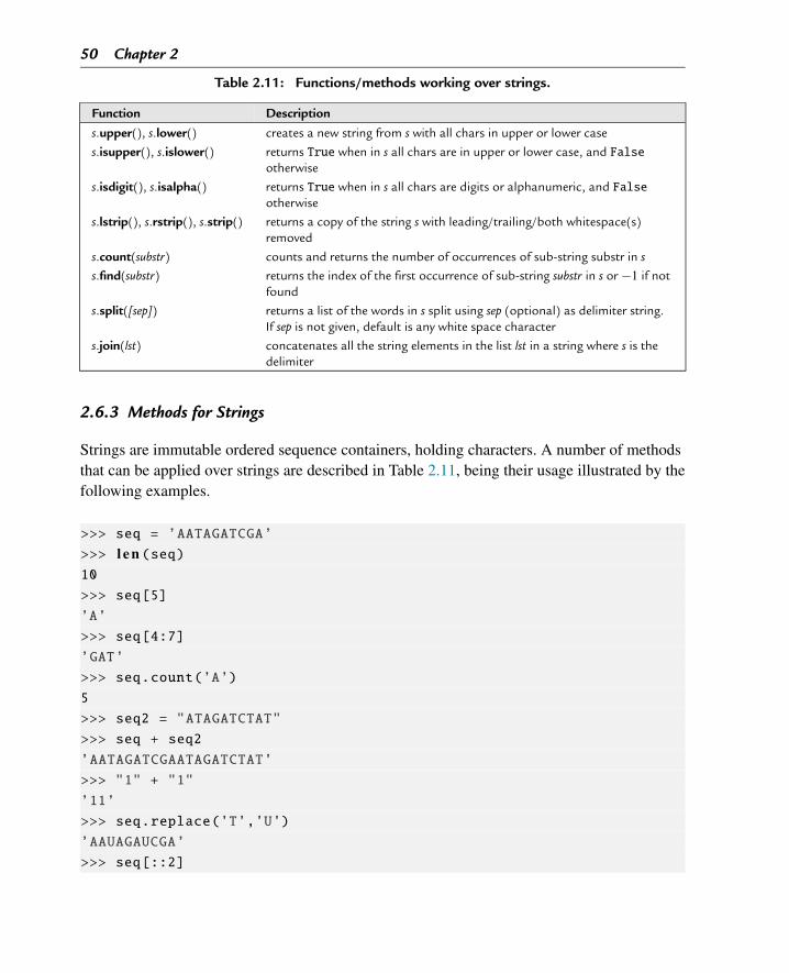
50 Chapter 2

Table 2.11: Functions/methods working over strings.

Function Description

s.upper(), s.lower() creates a new string from s with all chars in upper or lower case

s.isupper(), s.islower() returns True when in s all chars are in upper or lower case, and Falseotherwise

s.isdigit(), s.isalpha() returns True when in s all chars are digits or alphanumeric, and Falseotherwise

s.lstrip(), s.rstrip(), s.strip() returns a copy of the string s with leading/trailing/both whitespace(s)removed

s.count(substr) counts and returns the number of occurrences of sub-string substr in s

s.find(substr) returns the index of the first occurrence of sub-string substr in s or −1 if notfound

s.split([sep]) returns a list of the words in s split using sep (optional) as delimiter string.If sep is not given, default is any white space character

s.join(lst) concatenates all the string elements in the list lst in a string where s is thedelimiter

2.6.3 Methods for Strings

Strings are immutable ordered sequence containers, holding characters. A number of methodsthat can be applied over strings are described in Table 2.11, being their usage illustrated by thefollowing examples.

>>> seq = ’AATAGATCGA’

>>> l e n (seq)10

>>> seq[5]

’A’

>>> seq[4:7]

’GAT’

>>> seq.count(’A’)

5

>>> seq2 = "ATAGATCTAT"

>>> seq + seq2

’AATAGATCGAATAGATCTAT’

>>> "1" + "1"

’11’

>>> seq.replace(’T’,’U’)

’AAUAGAUCGA’

>>> seq[::2]

An Introduction to the Python Language 51

’ATGTG’

>>> seq[::−2]’ACAAA’

>>> seq[5:1:−2]’AA’

>>> seq.lower()

’aatagatcga’

>>> seq.lower()[2:]

’tagatcga’

>>> seq.lower()[2:].count(’c’)

1

>>> c = seq.count("C")

>>> g = seq.count("G")

>>> f l o a t (c + g)/ l e n (seq)∗10030.0

Some of these methods are particularly useful to identify matches within sequences, as shownbelow.

>>> "TAT" in "ATGATATATGA"

True>>> "TATC" in "ATGATATATGA"

F a l s e>>> seq = "ATGATATATGA"

>>> "TAT" in seq

True>>> "TATC" in seq

F a l s e>>> seq.find("TAT")

4

>>> seq.find("TATC")

−1>>> seq.count("TA")

2

>>> text = "Restriction enzymes work by recognizing a particular

sequence of bases on the DNA."

>>> text_tokens = text.split(" ")

>>> text_tokens

[’Restriction’, ’enzymes’, ’work’, ’by’, ’recognizing’, ’a’, ’

particular’, ’sequence’, ’of’, ’bases’, ’on’, ’the’, ’DNA.’]

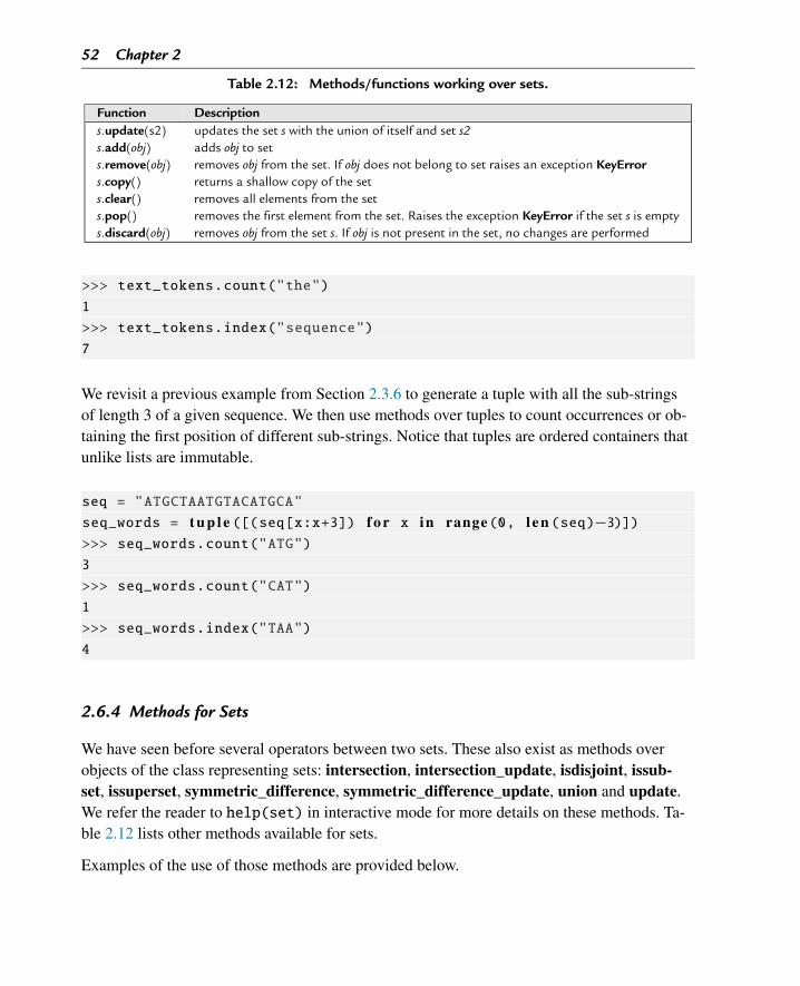
52 Chapter 2

Table 2.12: Methods/functions working over sets.

Function Descriptions.update(s2) updates the set s with the union of itself and set s2s.add(obj) adds obj to sets.remove(obj) removes obj from the set. If obj does not belong to set raises an exception KeyErrors.copy() returns a shallow copy of the sets.clear() removes all elements from the sets.pop() removes the first element from the set. Raises the exception KeyError if the set s is emptys.discard(obj) removes obj from the set s. If obj is not present in the set, no changes are performed

>>> text_tokens.count("the")

1

>>> text_tokens.index("sequence")

7

We revisit a previous example from Section 2.3.6 to generate a tuple with all the sub-stringsof length 3 of a given sequence. We then use methods over tuples to count occurrences or ob-taining the first position of different sub-strings. Notice that tuples are ordered containers thatunlike lists are immutable.

seq = "ATGCTAATGTACATGCA"

seq_words = t u p l e ([(seq[x:x+3]) f o r x in range(0, l e n (seq)−3)])>>> seq_words.count("ATG")

3

>>> seq_words.count("CAT")

1

>>> seq_words.index("TAA")

4

2.6.4 Methods for Sets

We have seen before several operators between two sets. These also exist as methods overobjects of the class representing sets: intersection, intersection_update, isdisjoint, issub-set, issuperset, symmetric_difference, symmetric_difference_update, union and update.We refer the reader to help(set) in interactive mode for more details on these methods. Ta-ble 2.12 lists other methods available for sets.

Examples of the use of those methods are provided below.

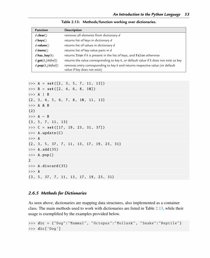
An Introduction to the Python Language 53

Table 2.13: Methods/function working over dictionaries.

Function Description

d.clear() removes all elements from dictionary d

d.keys() returns list of keys in dictionary d

d.values() returns list of values in dictionary d

d.items() returns list of key-value pairs in d

d.has_key(k) returns True if k is present in the list of keys, and False otherwise

d.get(k,[defval]) returns the value corresponding to key k, or default value if k does not exist as key

d.pop(k,[defval]) removes entry corresponding to key k and returns respective value (or defaultvalue if key does not exist)

>>> A = s e t ([2, 3, 5, 7, 11, 13])>>> B = s e t ([2, 4, 6, 8, 10])>>> A | B

{2, 3, 4, 5, 6, 7, 8, 10, 11, 13}

>>> A & B

{2}

>>> A − B

{3, 5, 7, 11, 13}

>>> C = s e t ([17, 19, 23, 31, 37])>>> A.update(C)

>>> A

{2, 3, 5, 37, 7, 11, 13, 17, 19, 23, 31}

>>> A.add(35)

>>> A.pop()

2

>>> A.discard(35)

>>> A

{3, 5, 37, 7, 11, 13, 17, 19, 23, 31}

2.6.5 Methods for Dictionaries

As seen above, dictionaries are mapping data structures, also implemented as a containerclass. The main methods used to work with dictionaries are listed in Table 2.13, while theirusage is exemplified by the examples provided below.

>>> dic = {"Dog":"Mammal", "Octopus":"Mollusk", "Snake":"Reptile"}

>>> dic[’Dog’]

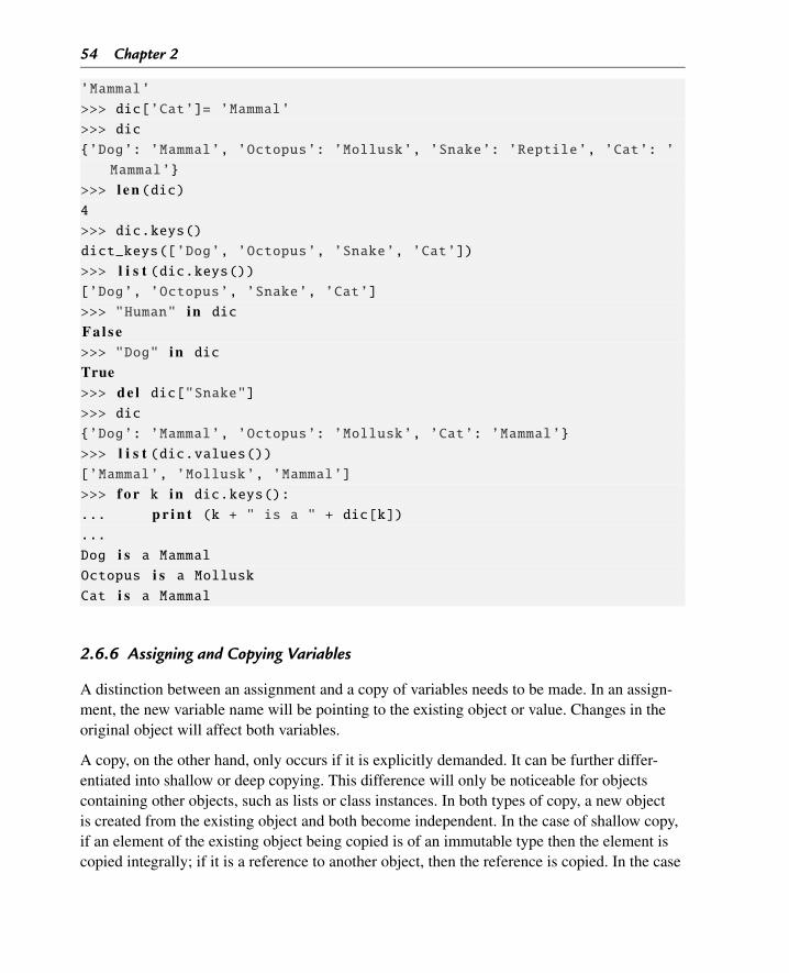
54 Chapter 2

’Mammal’

>>> dic[’Cat’]= ’Mammal’

>>> dic

{’Dog’: ’Mammal’, ’Octopus’: ’Mollusk’, ’Snake’: ’Reptile’, ’Cat’: ’

Mammal’}

>>> l e n (dic)4

>>> dic.keys()

dict_keys([’Dog’, ’Octopus’, ’Snake’, ’Cat’])

>>> l i s t (dic.keys())[’Dog’, ’Octopus’, ’Snake’, ’Cat’]

>>> "Human" in dic

F a l s e>>> "Dog" in dic

True>>> d e l dic["Snake"]>>> dic

{’Dog’: ’Mammal’, ’Octopus’: ’Mollusk’, ’Cat’: ’Mammal’}

>>> l i s t (dic.values())[’Mammal’, ’Mollusk’, ’Mammal’]

>>> f o r k in dic.keys():

... p r i n t (k + " is a " + dic[k])

...

Dog i s a MammalOctopus i s a MolluskCat i s a Mammal

2.6.6 Assigning and Copying Variables

A distinction between an assignment and a copy of variables needs to be made. In an assign-ment, the new variable name will be pointing to the existing object or value. Changes in theoriginal object will affect both variables.

A copy, on the other hand, only occurs if it is explicitly demanded. It can be further differ-entiated into shallow or deep copying. This difference will only be noticeable for objectscontaining other objects, such as lists or class instances. In both types of copy, a new objectis created from the existing object and both become independent. In the case of shallow copy,if an element of the existing object being copied is of an immutable type then the element iscopied integrally; if it is a reference to another object, then the reference is copied. In the case

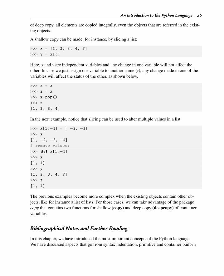
An Introduction to the Python Language 55

of deep copy, all elements are copied integrally, even the objects that are referred in the exist-ing objects.

A shallow copy can be made, for instance, by slicing a list:

>>> x = [1, 2, 3, 4, 7]

>>> y = x[:]

Here, x and y are independent variables and any change in one variable will not affect theother. In case we just assign our variable to another name (z), any change made in one of thevariables will affect the status of the other, as shown below.

>>> z = x

>>> z = x

>>> x.pop()

>>> z

[1, 2, 3, 4]

In the next example, notice that slicing can be used to alter multiple values in a list:

>>> x[1:−1] = [ −2, −3]>>> x

[1, −2, −3, −4]# remove values:

>>> d e l x[1:−1]>>> x

[1, 4]

>>> y

[1, 2, 3, 4, 7]

>>> z

[1, 4]

The previous examples become more complex when the existing objects contain other ob-jects, like for instance a list of lists. For those cases, we can take advantage of the packagecopy that contains two functions for shallow (copy) and deep copy (deepcopy) of containervariables.

Bibliographical Notes and Further Reading

In this chapter, we have introduced the most important concepts of the Python language.We have discussed aspects that go from syntax indentation, primitive and container built-in

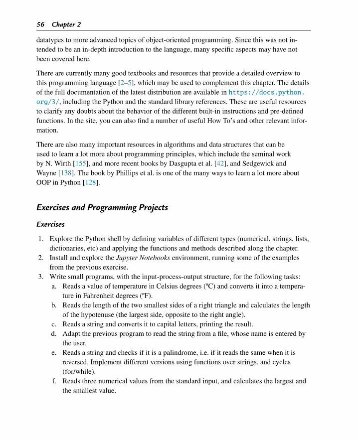
56 Chapter 2

datatypes to more advanced topics of object-oriented programming. Since this was not in-tended to be an in-depth introduction to the language, many specific aspects may have notbeen covered here.

There are currently many good textbooks and resources that provide a detailed overview tothis programming language [2–5], which may be used to complement this chapter. The detailsof the full documentation of the latest distribution are available in https://docs.python.org/3/, including the Python and the standard library references. These are useful resourcesto clarify any doubts about the behavior of the different built-in instructions and pre-definedfunctions. In the site, you can also find a number of useful How To’s and other relevant infor-mation.

There are also many important resources in algorithms and data structures that can beused to learn a lot more about programming principles, which include the seminal workby N. Wirth [155], and more recent books by Dasgupta et al. [42], and Sedgewick andWayne [138]. The book by Phillips et al. is one of the many ways to learn a lot more aboutOOP in Python [128].

Exercises and Programming Projects

Exercises

1. Explore the Python shell by defining variables of different types (numerical, strings, lists,dictionaries, etc) and applying the functions and methods described along the chapter.

2. Install and explore the Jupyter Notebooks environment, running some of the examplesfrom the previous exercise.

3. Write small programs, with the input-process-output structure, for the following tasks:a. Reads a value of temperature in Celsius degrees (ºC) and converts it into a tempera-

ture in Fahrenheit degrees (ºF).b. Reads the length of the two smallest sides of a right triangle and calculates the length

of the hypotenuse (the largest side, opposite to the right angle).c. Reads a string and converts it to capital letters, printing the result.d. Adapt the previous program to read the string from a file, whose name is entered by

the user.e. Reads a string and checks if it is a palindrome, i.e. if it reads the same when it is

reversed. Implement different versions using functions over strings, and cycles(for/while).

f. Reads three numerical values from the standard input, and calculates the largest andthe smallest value.

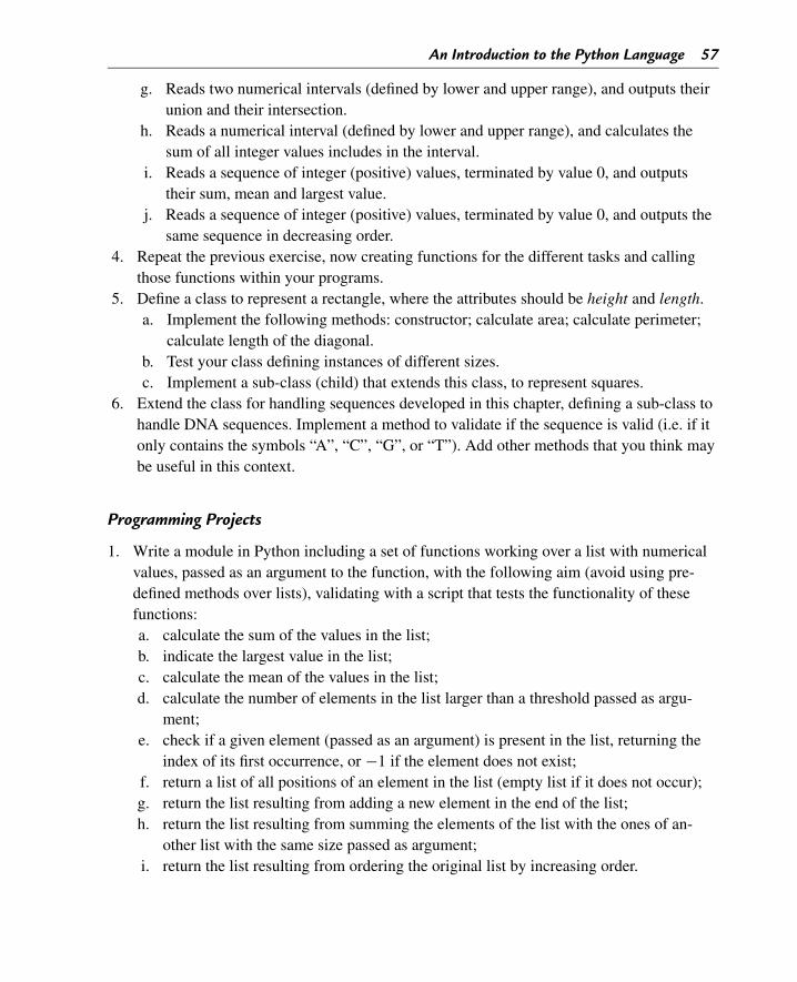
An Introduction to the Python Language 57

g. Reads two numerical intervals (defined by lower and upper range), and outputs theirunion and their intersection.

h. Reads a numerical interval (defined by lower and upper range), and calculates thesum of all integer values includes in the interval.

i. Reads a sequence of integer (positive) values, terminated by value 0, and outputstheir sum, mean and largest value.

j. Reads a sequence of integer (positive) values, terminated by value 0, and outputs thesame sequence in decreasing order.

4. Repeat the previous exercise, now creating functions for the different tasks and callingthose functions within your programs.

5. Define a class to represent a rectangle, where the attributes should be height and length.a. Implement the following methods: constructor; calculate area; calculate perimeter;

calculate length of the diagonal.b. Test your class defining instances of different sizes.c. Implement a sub-class (child) that extends this class, to represent squares.

6. Extend the class for handling sequences developed in this chapter, defining a sub-class tohandle DNA sequences. Implement a method to validate if the sequence is valid (i.e. if itonly contains the symbols “A”, “C”, “G”, or “T”). Add other methods that you think maybe useful in this context.

Programming Projects

1. Write a module in Python including a set of functions working over a list with numericalvalues, passed as an argument to the function, with the following aim (avoid using pre-defined methods over lists), validating with a script that tests the functionality of thesefunctions:a. calculate the sum of the values in the list;b. indicate the largest value in the list;c. calculate the mean of the values in the list;d. calculate the number of elements in the list larger than a threshold passed as argu-

ment;e. check if a given element (passed as an argument) is present in the list, returning the

index of its first occurrence, or −1 if the element does not exist;f. return a list of all positions of an element in the list (empty list if it does not occur);g. return the list resulting from adding a new element in the end of the list;h. return the list resulting from summing the elements of the list with the ones of an-

other list with the same size passed as argument;i. return the list resulting from ordering the original list by increasing order.

58 Chapter 2

2. Write a module in Python including a set of functions working over matrices. The ma-trix (represented as a list of lists) will be passed as the first argument. Some functions toinclude may be the following:a. calculate the sum of the values in the matrix;b. indicate the largest (smallest) value in the matrix;c. calculate the mean of the values in the matrix;d. calculate the mean (or sum) of the values in each row (or column); the result should

be a list;e. calculate the multiplication of the values in the diagonal;f. check if the matrix is square (same number of rows and columns);g. multiply all elements by a numerical value, returning another matrix;h. add two matrices (assuming they have the same dimension);i. multiply two matrices.

3. Develop a class to keep numerical matrices. The attributes of the class should be thenumber of rows, number of columns, and a list of lists keeping the elements of the ma-trix. Implement a constructor to create an empty matrix given the number of rows andcolumns. Implement methods with a functionality similar to the ones listed in the previousquestion.

CHAPTER 3

Cellular and Molecular BiologyFundamentalsIn this chapter, we review the major concepts in cellular and molecular Biology relevant forthe Bioinformatics algorithms covered in this book. These fields look inside the cell and try tounderstand its mechanisms by studying how its molecular components co-exist and interact.We will start by providing an overview on the composition and organization of cells and theirdifferent types. Then, we will discuss characteristics of the genetic material and how the ge-netic information flows along different cellular processes. Next, we present the notion of gene,a discrete unit of genetic information and discuss details of its codification in the genetic ma-terial. We provide an outline of the major milestones in the history of the human genome andgive examples on how its study is providing us insights in the understanding of human diver-sity and disease. Finally, we address some important resources on biological data in particularfor biological sequences.

3.1 The Cell: The Basic Unit of Life

Cells are the basic units of life. All living things are made of cells. In organisms like plants oranimals, the first cell of an organism, called the primordial germ cell, is obtained by the fusionof the sperm and the egg that are contributed by the parents. This first cell undergoes multiplerounds of division and differentiation, resulting in cells of different nature. This way, each cellwill derive from another cell and contain all the necessary information to replicate itself.

Some features are common to all cells, but, in multicellular organisms as humans, through dif-ferentiation mechanisms, many different cell types arise, eventually showing very distinctcharacteristics. Cells of a given type have similar functions and aggregate to form tissues.Tissues reflect their cell type composition and can also be very distinct between them. Forinstance, kidney or heart are very distinct tissues from skin or stomach. Organs are made oftissues and shape the complexity and aspect of a complex organism. Multicellular organisms,which include animals, plants or most fungi, are the combined result of many cells. But not allorganisms have many cells. In fact, unicellular organisms, such as Saccharomyces cerevisiae,a fungi also known as the budding or baker’s yeast, or bacteria only contain one cell.

A cell is mostly composed by water. For instance, a bacterial cell has a composition by weightof approximately 70% of water and 30% of chemical origin. From these, 7% are small-

Bioinformatics Algorithms. DOI: 10.1016/B978-0-12-812520-5.00003-1Copyright © 2018 Elsevier Inc. All rights reserved. 59

60 Chapter 3

molecules including amino acids and nucleotides and 23% are macro-molecules includingproteins, lipids or polysaccharides [120].

According to their internal structure, cells can be divided in two major categories: prokaryoticcells, that have no nucleus or internal membranes, and eukaryotic cells that have a defined nu-cleus, internal membranes and functional elements called organelles that have varying shapesand size and play specific functions.

The cell type is the factor that drives organism categorization as prokaryotes or eukaryotes.Most of the unicellular organisms are prokaryotes, including bacteria and archea species. But,eukaryotic unicellular organisms also exist. Several fungi species, such as Saccharomycescerevisiae or Schizosaccharomyces pombe are good examples. The more complex multicellu-lar species are all eukaryotes.

At the structural level, all cells are surrounded by a structure called cell membrane or plasmamembrane. This membrane is permeable to molecules that cells need to absorb from or ex-crete to the outside medium. Within the cell, we find the cytoplasm, a gel-like substance,largely composed of water, which serves as the medium for the cell.

Among the molecules with a biological role, we can find nucleic acids. These encode and ex-press the genetic code that is kept within the cell. There are two major types of nucleic acids:deoxyribonucleic acid (DNA) and ribonucleic acid (RNA). As we will see, although chem-ically very similar, these molecules have different purposes. DNA contains the informationnecessary to build a cell and keep it functioning. In eukaryotic cells, DNA will be found in thenucleus, while in prokaryotic cells it will be in the cytoplasm. By reflecting the informationencoded in the DNA, the RNA will be used as an intermediate in the definition of the compo-sition and, therefore, the nature of the cell.

Amino acids are another important type of bio-molecule. They are the building blocks of pro-teins, which are macromolecules that perform most of the functions in the cell. Proteins havea broad range of functions, spanning from catalytic to structural functions. Enzymes, for in-stance, are a type of abundant proteins that promote chemical reactions, and convert certainmolecules into other types of molecules required for the functioning of the cell. Other im-portant organic macromolecules include: carbohydrates that serve as energy storage, both forimmediate or long-term energy demands; and, lipids that are part of the plasma membraneand their function involves signaling and energy storage.

The cell also contains other components of varying complexity. Of notice, the mitochondriaand the chloroplasts, which are organelles involved in the production of energy and the ribo-somes that are large and complex molecules composed by a mixture of genetic material. Theirfunction is to assemble proteins and, as we will see later, they play a central role in the flow ofgenetic information.

Cellular and Molecular Biology Fundamentals 61

3.2 Genetic Information: Nucleic Acids

The DNA is a polymer composed of four nucleic acid units, called nucleotides or base pairs.Nucleotides have a similar chemical composition, but can be distinguished by the respectivenitrogenous bases: Adenine, Guanine, Thymine or Cytosine. Adenine and Guanine are partof the purines group, while Cytosine and Thymine are pyrimidines. Nucleotides are usuallyreferred by their first letter: A, G, T or C.

The DNA is a molecule composed of two complementary strands that form and stick togetherdue to the connections established between the nucleotides in both strands. This comple-mentarity is possible due to a chemical phenomenon where Adenine bonds only to Thyminenucleotides as a result of two hydrogen connections (A = T ), and Guanine bonds only to Cy-tosine by three hydrogen bonds (C ≡ G). This results in two complementary and anti-parallelstrands (connected in opposite directions). Knowing the sequence of the nucleotides in oneof the strands it is possible to obtain the sequence in the opposite strand by taking the com-plement of its nucleotides. The two opposite strands are also read in reverse directions, andtherefore we say that one strand is the reverse complement of the other. The existence of thesetwo strands is essential for passing the genetic information to new cells and to produce pro-teins. Due to this complementarity and redundancy, it is therefore standard to describe theDNA through only one of its strand sequences using the four-letter alphabet: {A, G, T, C}.

DNA molecules can form sequences of hundreds of thousands or millions of nucleotides.Each of these individual and long DNA molecules are called chromosomes. Within chromo-somes, we find genes that are functional regions of the DNA and encode the instructions tomake proteins. The complete set of DNA forms the genetic material of the organism and iscalled genome. The size of the genome and the corresponding number of chromosomes ina cell is variable and depends on the species. For instance, certain bacterial species have agenome that contains around a few hundred or a few million base pairs in a single chromo-some, while mice or humans have a genome with approximately 3 billion (3 × 109) base pairs,but there are other species with even larger genomes.

An organism or a cell is haploid if it only contains a single set of unpaired chromosomes.If it contains two complete sets of chromosomes it is called diploid. Humans, for instance,are diploids and contain 23 chromosome pairs. The twenty-third chromosome pair (sexualchromosome) determines the gender of the individual. If it contains two copies of the X chro-mosome, it results in a female, while if it contains a chromosome X and chromosome Y, itresults in a male individual. So, in total, the human genome has 24 distinct chromosomes.The remaining 22 chromosome pairs are called autosomal chromosomes. Each chromo-some contains many genes, and in the human genome they can sum up to nearly 21,000coding for proteins. As we will see later, different types of genes can be found in the humangenome.

62 Chapter 3

Depending on the type of the cell, the genome is organized differently. In a prokaryotic cell,the genome exists in the form of a circular chromosome and it is located in the cytoplasm. Onthe other hand, in an eukaryotic cell, the genome is found in the nucleus and tightly packedinto linear chromosomes. The chromosome organization is highly hierarchical and consistsof a DNA-protein complex called chromatin, that is organized in an array of sub-units callednucleosomes. In these intermediate sub-structures, the DNA structure wraps around proteinscalled histones. This organization allows accommodating a long DNA molecule in a smallspace. It also provides a structure to regulate the expression of genes.

The genetic composition of an organism comprised on its genome is called the genotype. Thephenotype is the set of physical and observable traits of an individual. It results from the com-bination of the genotype and the environment. The height of an individual or the color of theeyes are phenotypic traits that are totally or partially encoded on the genotype.

In most multicellular organisms, each cell contains the same genetic information. At a certainpoint, the cell divides into two daughter cells, passing a copy of its DNA to each of its childcells. The process of copying the DNA is called DNA replication. It is important that this pro-cess is accurate to ensure that the new cells contain the same genetic material of the motherand result in healthy cells. Since DNA has a double-helix structure, for DNA replication totake place, it is necessary that the two strands separate. Then, proteins (enzymes) called DNApolymerases will synthesize a new DNA strand by adding nucleotides that complement eachof the nucleotides in the original strand, also called the template strand.

So far, we have seen that the DNA contains the genetic information required for the cells tofunction and replicate and that genes, which are regions found along the DNA, encode theinformation necessary to synthesize proteins and other molecular products. The process ofusing the information encoded in a gene to produce a functional gene product is called geneexpression. But, what we have not discussed yet, is how the information flows from DNA toproteins. DNA, RNA and proteins are the central elements on this flow of genetic informa-tion that occurs in two steps: transcription and translation, in what is also called the centraldogma of molecular and cell Biology.

RNA is a single strand molecule that in contrast to DNA does not form an helix structure. Itis also composed of four nucleotides, but it contains a fifth type of nucleic acid called Uracil(U) that is not present in the DNA. So, while thymine only exists in DNA, uracil is only foundin RNA. The other three bases are common to DNA and RNA. The sequence alphabet of theRNA is: {A, G, U, C}.

3.2.1 Transcription: RNA Synthesis

Transcription is the first step required to produce a protein. In this step, the nucleotide se-quence of a gene from one of the DNA strands is transcribed, i.e. copied into a complemen-

Cellular and Molecular Biology Fundamentals 63

tary molecule of RNA. The complementarity of the genetic code allows recovering theinformation encoded in the original DNA sequence, a process performed by an enzyme calledRNA polymerase. Additional steps of RNA processing, including stabilizing the elements atthe end of the molecule, are performed by different protein complexes.

After these steps, which occur within the nucleus of the cell, an RNA molecule called maturemessenger RNA or mRNA is obtained. The mature mRNA is then transported to the cytoplasm,where it will be used by the cellular machine to guide the production of a protein. Fig. 3.1depicts the different steps involved in the flow of genetic information, including transcriptionand translation, covered in the next section, as well as replication, aforementioned.

3.2.2 Translation: Protein Synthesis

Proteins are cellular entities that have either a structural function, participating in the physicaldefinition of the cell, or a chemical function being involved in chemical reactions occur-ring in the cell. In order to function as expected, a protein needs to acquire the appropriatestructure. This structure is often decomposed at different complexity levels. The primarystructure is defined by the chain of amino acids and is called a polypeptide. These polypep-tides will coil and fold, forming regular and local sub-structures, called secondary structuresof the protein. One or more combined polypeptides with the appropriate structure will forma fully functional protein. It is the sequence of amino acids and the current cellular condi-tions that will determine how the polypeptide will fold and the protein acquires its struc-ture.

Translation is the process in which the nucleotide sequence of an mRNA molecule is tran-scribed into a chain of amino acids forming a polypeptide, that will consist in part or the to-tality of a protein. This process is performed by the ribosomes that attach and scan the mRNAfrom one end to the other, in groups of nucleotide triplets or codons. In each position of thetriplet, we have one of four nucleotides, so there are 4 × 4 × 4 = 64 possible triplets. To eachcodon in the mRNA sequence corresponds an amino acid in the polypeptide chain. Some ofthese codons represent specific signals that indicate the initiation or the termination of thetranslation process. Once the ribosome detects an initiation codon, it starts the formation ofthe amino acid chain, and when it scans the stop codon it stops the translation and detachesfrom the mRNA molecule.

There are 20 types of amino acids used to form polypeptides, much less than the 64 possiblecodons. Therefore, more than one codon corresponds to a type of amino acid. This mappingbetween codons and amino acids is provided in Table 3.1 and is commonly called geneticcode.

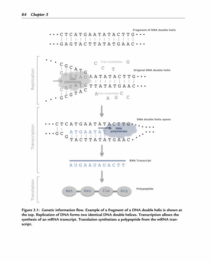
64 Chapter 3

Figure 3.1: Genetic information flow. Example of a fragment of a DNA double helix is shown atthe top. Replication of DNA forms two identical DNA double helices. Transcription allows thesynthesis of an mRNA transcript. Translation synthetizes a polypeptide from the mRNA tran-script.

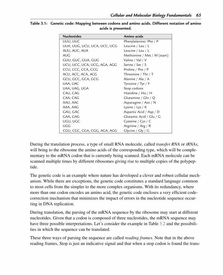
Cellular and Molecular Biology Fundamentals 65

Table 3.1: Genetic code: Mapping between codons and amino acids. Different notation of aminoacids is presented.

Nucleotides Amino acidsUUU, UUC Phenylalanine/ Phe / PUUA, UUG, UCU, UCA, UCC, UCG Leucine / Leu / LAUU, AUC, AUA Leucine / Leu / LAUG Methionine / Met / M (start)GUU, GUC, GUA, GUG Valine / Val / VUCU, UCC, UCA, UCG, AGA, AGG Serine / Ser / SCCU, CCC, CCA, CCG Proline / Pro / PACU, ACC, ACA, ACG Threonine / Thr / TGCU, GCC, GCA, GCG Alanine / Ala / AUAA, UAC Tyrosine / Tyr / YUAA, UAG, UGA Stop codonsCAU, CAG Histidine / His / HCAA, CAG Glutamine / Gln / QAAU, AAC Asparagine / Asn / NAAA, AAG Lysine / Lys / KGAU, GAC Aspartic Acid / Asp / DGAA, GAG Glutamic Acid / Glu / GUGU, UGC Cysteine / Cys / CUGG Arginine / Arg / RCGU, CGC, CGA, CGG, AGA, AGG Glycine / Gly / G

During the translation process, a type of small RNA molecule, called transfer RNA or tRNAs,will bring to the ribosome the amino acids of the corresponding type, which will be comple-mentary to the mRNA codon that is currently being scanned. Each mRNA molecule can bescanned multiple times by different ribosomes giving rise to multiple copies of the polypep-tide.

The genetic code is an example where nature has developed a clever and robust cellular mech-anism. While there are exceptions, the genetic code constitutes a standard language commonto most cells from the simpler to the more complex organisms. With its redundancy, wheremore than one codon encodes an amino acid, the genetic code encloses a very efficient code-correction mechanism that minimizes the impact of errors in the nucleotide sequence occur-ring in DNA replication.

During translation, the parsing of the mRNA sequence by the ribosome may start at differentnucleotides. Given that a codon is composed of three nucleotides, the mRNA sequence mayhave three possible interpretations. Let’s consider the example in Table 3.2 and the possibili-ties in which the sequence can be translated.

These three ways of parsing the sequence are called reading frames. Note that in the abovereading frames, Stop is just an indicative signal and that when a stop codon is found the trans-

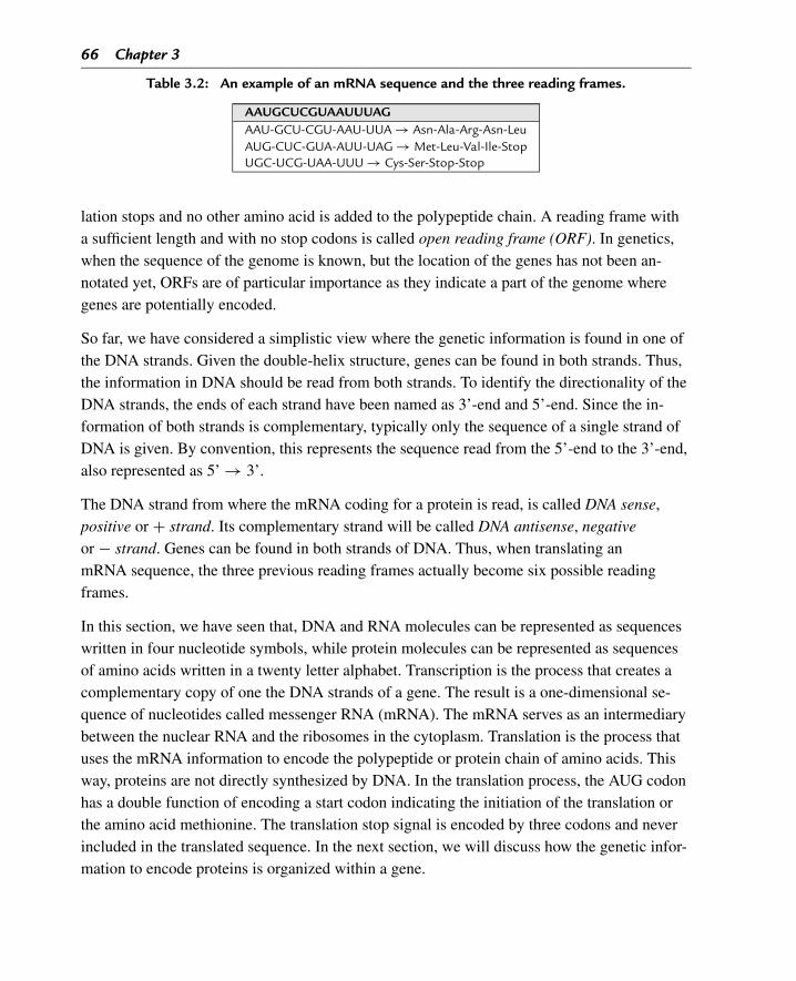
66 Chapter 3

Table 3.2: An example of an mRNA sequence and the three reading frames.

AAUGCUCGUAAUUUAGAAU-GCU-CGU-AAU-UUA → Asn-Ala-Arg-Asn-LeuAUG-CUC-GUA-AUU-UAG → Met-Leu-Val-Ile-StopUGC-UCG-UAA-UUU → Cys-Ser-Stop-Stop

lation stops and no other amino acid is added to the polypeptide chain. A reading frame witha sufficient length and with no stop codons is called open reading frame (ORF). In genetics,when the sequence of the genome is known, but the location of the genes has not been an-notated yet, ORFs are of particular importance as they indicate a part of the genome wheregenes are potentially encoded.

So far, we have considered a simplistic view where the genetic information is found in one ofthe DNA strands. Given the double-helix structure, genes can be found in both strands. Thus,the information in DNA should be read from both strands. To identify the directionality of theDNA strands, the ends of each strand have been named as 3’-end and 5’-end. Since the in-formation of both strands is complementary, typically only the sequence of a single strand ofDNA is given. By convention, this represents the sequence read from the 5’-end to the 3’-end,also represented as 5’ → 3’.

The DNA strand from where the mRNA coding for a protein is read, is called DNA sense,positive or + strand. Its complementary strand will be called DNA antisense, negativeor − strand. Genes can be found in both strands of DNA. Thus, when translating anmRNA sequence, the three previous reading frames actually become six possible readingframes.

In this section, we have seen that, DNA and RNA molecules can be represented as sequenceswritten in four nucleotide symbols, while protein molecules can be represented as sequencesof amino acids written in a twenty letter alphabet. Transcription is the process that creates acomplementary copy of one the DNA strands of a gene. The result is a one-dimensional se-quence of nucleotides called messenger RNA (mRNA). The mRNA serves as an intermediarybetween the nuclear RNA and the ribosomes in the cytoplasm. Translation is the process thatuses the mRNA information to encode the polypeptide or protein chain of amino acids. Thisway, proteins are not directly synthesized by DNA. In the translation process, the AUG codonhas a double function of encoding a start codon indicating the initiation of the translation orthe amino acid methionine. The translation stop signal is encoded by three codons and neverincluded in the translated sequence. In the next section, we will discuss how the genetic infor-mation to encode proteins is organized within a gene.

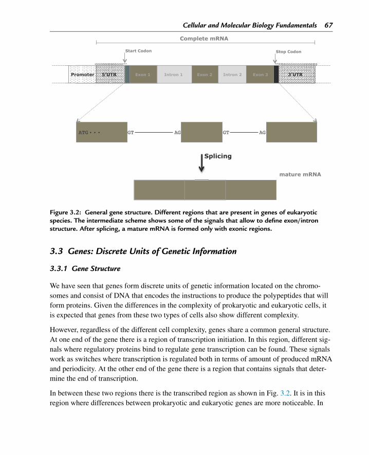
Cellular and Molecular Biology Fundamentals 67

Figure 3.2: General gene structure. Different regions that are present in genes of eukaryoticspecies. The intermediate scheme shows some of the signals that allow to define exon/intronstructure. After splicing, a mature mRNA is formed only with exonic regions.

3.3 Genes: Discrete Units of Genetic Information

3.3.1 Gene Structure

We have seen that genes form discrete units of genetic information located on the chromo-somes and consist of DNA that encodes the instructions to produce the polypeptides that willform proteins. Given the differences in the complexity of prokaryotic and eukaryotic cells, itis expected that genes from these two types of cells also show different complexity.

However, regardless of the different cell complexity, genes share a common general structure.At one end of the gene there is a region of transcription initiation. In this region, different sig-nals where regulatory proteins bind to regulate gene transcription can be found. These signalswork as switches where transcription is regulated both in terms of amount of produced mRNAand periodicity. At the other end of the gene there is a region that contains signals that deter-mine the end of transcription.

In between these two regions there is the transcribed region as shown in Fig. 3.2. It is in thisregion where differences between prokaryotic and eukaryotic genes are more noticeable. In

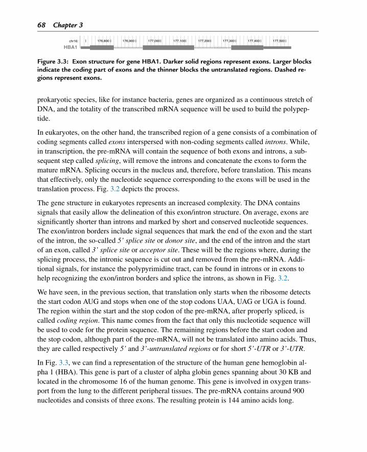
68 Chapter 3

Figure 3.3: Exon structure for gene HBA1. Darker solid regions represent exons. Larger blocksindicate the coding part of exons and the thinner blocks the untranslated regions. Dashed re-gions represent exons.

prokaryotic species, like for instance bacteria, genes are organized as a continuous stretch ofDNA, and the totality of the transcribed mRNA sequence will be used to build the polypep-tide.

In eukaryotes, on the other hand, the transcribed region of a gene consists of a combination ofcoding segments called exons interspersed with non-coding segments called introns. While,in transcription, the pre-mRNA will contain the sequence of both exons and introns, a sub-sequent step called splicing, will remove the introns and concatenate the exons to form themature mRNA. Splicing occurs in the nucleus and, therefore, before translation. This meansthat effectively, only the nucleotide sequence corresponding to the exons will be used in thetranslation process. Fig. 3.2 depicts the process.

The gene structure in eukaryotes represents an increased complexity. The DNA containssignals that easily allow the delineation of this exon/intron structure. On average, exons aresignificantly shorter than introns and marked by short and conserved nucleotide sequences.The exon/intron borders include signal sequences that mark the end of the exon and the startof the intron, the so-called 5’ splice site or donor site, and the end of the intron and the startof an exon, called 3’ splice site or acceptor site. These will be the regions where, during thesplicing process, the intronic sequence is cut out and removed from the pre-mRNA. Addi-tional signals, for instance the polypyrimidine tract, can be found in introns or in exons tohelp recognizing the exon/intron borders and splice the introns, as shown in Fig. 3.2.

We have seen, in the previous section, that translation only starts when the ribosome detectsthe start codon AUG and stops when one of the stop codons UAA, UAG or UGA is found.The region within the start and the stop codon of the pre-mRNA, after properly spliced, iscalled coding region. This name comes from the fact that only this nucleotide sequence willbe used to code for the protein sequence. The remaining regions before the start codon andthe stop codon, although part of the pre-mRNA, will not be translated into amino acids. Thus,they are called respectively 5’ and 3’-untranslated regions or for short 5’-UTR or 3’-UTR.

In Fig. 3.3, we can find a representation of the structure of the human gene hemoglobin al-pha 1 (HBA). This gene is part of a cluster of alpha globin genes spanning about 30 KB andlocated in the chromosome 16 of the human genome. This gene is involved in oxygen trans-port from the lung to the different peripheral tissues. The pre-mRNA contains around 900nucleotides and consists of three exons. The resulting protein is 144 amino acids long.

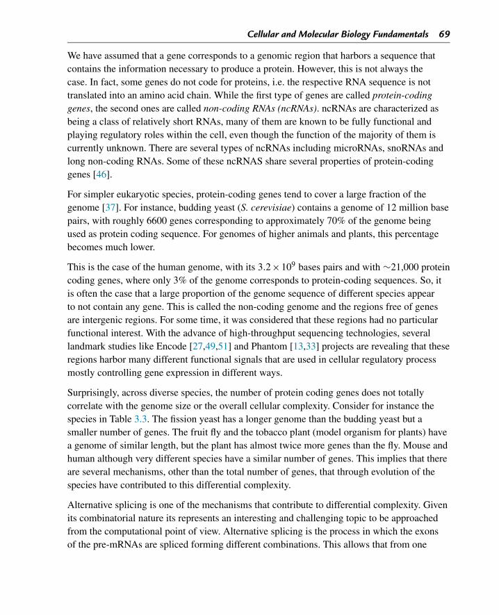
Cellular and Molecular Biology Fundamentals 69

We have assumed that a gene corresponds to a genomic region that harbors a sequence thatcontains the information necessary to produce a protein. However, this is not always thecase. In fact, some genes do not code for proteins, i.e. the respective RNA sequence is nottranslated into an amino acid chain. While the first type of genes are called protein-codinggenes, the second ones are called non-coding RNAs (ncRNAs). ncRNAs are characterized asbeing a class of relatively short RNAs, many of them are known to be fully functional andplaying regulatory roles within the cell, even though the function of the majority of them iscurrently unknown. There are several types of ncRNAs including microRNAs, snoRNAs andlong non-coding RNAs. Some of these ncRNAS share several properties of protein-codinggenes [46].

For simpler eukaryotic species, protein-coding genes tend to cover a large fraction of thegenome [37]. For instance, budding yeast (S. cerevisiae) contains a genome of 12 million basepairs, with roughly 6600 genes corresponding to approximately 70% of the genome beingused as protein coding sequence. For genomes of higher animals and plants, this percentagebecomes much lower.

This is the case of the human genome, with its 3.2×109 bases pairs and with ∼21,000 proteincoding genes, where only 3% of the genome corresponds to protein-coding sequences. So, itis often the case that a large proportion of the genome sequence of different species appearto not contain any gene. This is called the non-coding genome and the regions free of genesare intergenic regions. For some time, it was considered that these regions had no particularfunctional interest. With the advance of high-throughput sequencing technologies, severallandmark studies like Encode [27,49,51] and Phantom [13,33] projects are revealing that theseregions harbor many different functional signals that are used in cellular regulatory processmostly controlling gene expression in different ways.

Surprisingly, across diverse species, the number of protein coding genes does not totallycorrelate with the genome size or the overall cellular complexity. Consider for instance thespecies in Table 3.3. The fission yeast has a longer genome than the budding yeast but asmaller number of genes. The fruit fly and the tobacco plant (model organism for plants) havea genome of similar length, but the plant has almost twice more genes than the fly. Mouse andhuman although very different species have a similar number of genes. This implies that thereare several mechanisms, other than the total number of genes, that through evolution of thespecies have contributed to this differential complexity.

Alternative splicing is one of the mechanisms that contribute to differential complexity. Givenits combinatorial nature its represents an interesting and challenging topic to be approachedfrom the computational point of view. Alternative splicing is the process in which the exonsof the pre-mRNAs are spliced forming different combinations. This allows that from one

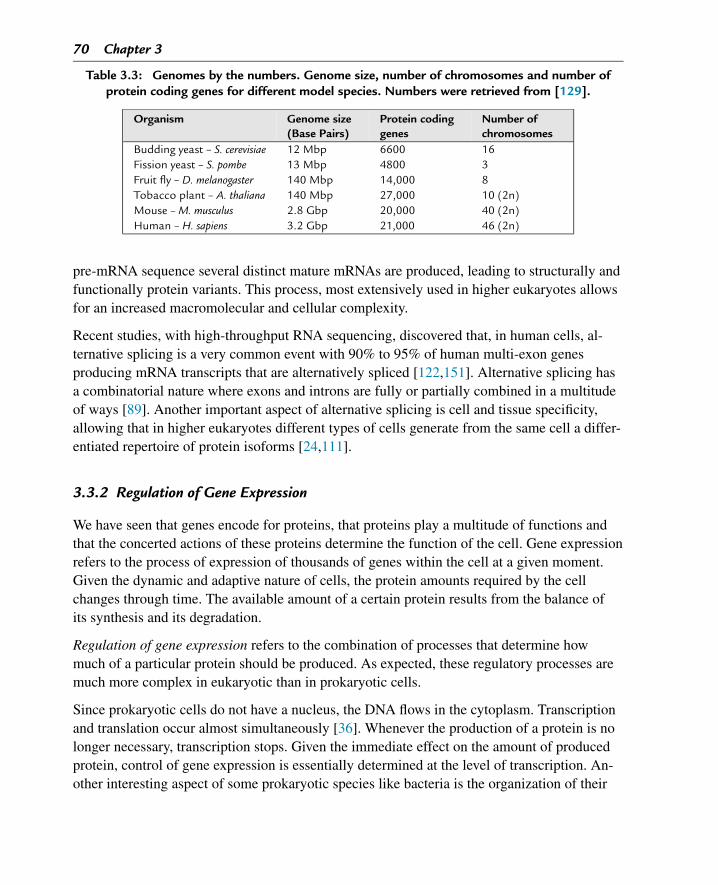
70 Chapter 3

Table 3.3: Genomes by the numbers. Genome size, number of chromosomes and number ofprotein coding genes for different model species. Numbers were retrieved from [129].

Organism Genome size(Base Pairs)

Protein codinggenes

Number ofchromosomes

Budding yeast – S. cerevisiae 12 Mbp 6600 16Fission yeast – S. pombe 13 Mbp 4800 3Fruit fly – D. melanogaster 140 Mbp 14,000 8Tobacco plant – A. thaliana 140 Mbp 27,000 10 (2n)Mouse – M. musculus 2.8 Gbp 20,000 40 (2n)Human – H. sapiens 3.2 Gbp 21,000 46 (2n)

pre-mRNA sequence several distinct mature mRNAs are produced, leading to structurally andfunctionally protein variants. This process, most extensively used in higher eukaryotes allowsfor an increased macromolecular and cellular complexity.

Recent studies, with high-throughput RNA sequencing, discovered that, in human cells, al-ternative splicing is a very common event with 90% to 95% of human multi-exon genesproducing mRNA transcripts that are alternatively spliced [122,151]. Alternative splicing hasa combinatorial nature where exons and introns are fully or partially combined in a multitudeof ways [89]. Another important aspect of alternative splicing is cell and tissue specificity,allowing that in higher eukaryotes different types of cells generate from the same cell a differ-entiated repertoire of protein isoforms [24,111].

3.3.2 Regulation of Gene Expression

We have seen that genes encode for proteins, that proteins play a multitude of functions andthat the concerted actions of these proteins determine the function of the cell. Gene expressionrefers to the process of expression of thousands of genes within the cell at a given moment.Given the dynamic and adaptive nature of cells, the protein amounts required by the cellchanges through time. The available amount of a certain protein results from the balance ofits synthesis and its degradation.

Regulation of gene expression refers to the combination of processes that determine howmuch of a particular protein should be produced. As expected, these regulatory processes aremuch more complex in eukaryotic than in prokaryotic cells.

Since prokaryotic cells do not have a nucleus, the DNA flows in the cytoplasm. Transcriptionand translation occur almost simultaneously [36]. Whenever the production of a protein is nolonger necessary, transcription stops. Given the immediate effect on the amount of producedprotein, control of gene expression is essentially determined at the level of transcription. An-other interesting aspect of some prokaryotic species like bacteria is the organization of their

Cellular and Molecular Biology Fundamentals 71

genes in clusters of co-regulated genes, called operons. Genes from an operon are close inthe genome and under a common control mechanism that allows them to be transcribed in acoordinated way. This gives the species the capacity to rapidly react to different external stim-uli [131].

In eukaryotic cells, gene regulation is a multi-step process controlled by multiple mecha-nisms. Given that transcription and translation are decoupled, regulation may occur in thenucleus during transcription and RNA processing or in the cytoplasm during translation. Itmay even occur after the protein being produced, where biochemical modifications to the pro-tein result in post-translational regulation [36,131].

3.4 Human Genome

We will now focus a little bit on our species. The human body contains an estimated numberof 75 to 100 trillion (1012) cells [120,129]. Each cell contains a genome and apart from someabnormalities like for instance cancer, the genetic information carried throughout all the so-matic cells is the same. Humans have diploid cells with two copies of each chromosome.

As seen before, human somatic cells contain 46 chromosomes, consisting of two sets of 23chromosomes. Male and Female individuals are distinguished by the thirty-third chromosomeset. While females have two copies of chromosome X, males have a copy of chromosomeX and a copy of chromosome Y. Each chromosome contains an array of genes. Current esti-mates point to approximately 21,000 protein-coding genes. Nevertheless, other types of geneshave been discovered and current gene annotation efforts annotate more than 50,000 genes inthe human genome [72].

The history of modern genetics started more than 150 years ago with the pioneering workof the botanist and scientist Gregor Mendel [121]. He has been considered the father of themodern genetics due to its discoveries of the basic principles of heredity made through experi-ments in plant hybridization. In the middle of the 20th century, the work of Rosalind Franklin,Maurice Wilkins, James Watson and Francis Crick revealed the double helix structure of theDNA. This was a major breakthrough that boosted the research on the human genome. In1961, Marshall Nirenberg deciphered the genetic code for protein synthesis that we have seenin Table 3.1.

In the late 1970’s and early 1980’s, two techniques have revolutionized modern molecularbiology. These were the rapid DNA sequencing technique developed by Frederick Sanger andpolymerase chain reaction (PCR) for DNA amplification by Kary Mullis. Also, during thisperiod, the first genetic diseases started to be mapped.

72 Chapter 3

The Human Genome Project started in 1990. The goal was to characterize both physicallyand functionally the human genome. Its impact on so many different aspects of human lifemakes it one of the greatest achievements of human history. In 1998, the Celera GenomicsCorporation joins the race of sequencing the human genome in an effort lead by Craig Venter.In 1999, chromosome 22 was the first human chromosome to be sequenced.

During this time, other efforts were also being made to sequence other species. In 1995,Haemophilus influenzae was the first bacterium to have its genome sequenced. Early years ofthe decade of 2000 were exciting years for molecular biology. In 2000, the genome sequenceof the model organism fruit fly was released, followed by the first draft of the human genomein 2001. In 2002, the mouse model organism was the first mammalian to have its genome se-quence revealed and in 2003 a more complete version of the human genome was announcedwith the end of this project.

Since then, improvements have been made to the genome sequence. Other large-scale inter-national efforts have helped us to better understand the human genome. Examples of suchprojects include the ENCODE Project [27,49,51] that had the goal of providing a detailedview of the functional elements in the human genome and the 1000 Genomes Project [15] thatmapped the genetic variation in humans.

Despite certain phenotypic differences that humans may have, like height, color of the skin,hair or color of the eyes, we are all very similar at the genetic level. In fact, on average, anytwo humans share more than 99% of their DNA sequence [98] with the amount of geneticvariation due to differences in populations being modest [156]. The remaining fraction of thegenome that varies is important, since in combination with the environment is what makes usunique. There are different ways in which this variation can occur.

Point mutations that consist in the change of one nucleotide by another are the most frequenttype of genomic alteration. When they occur with a certain frequency, for instance in morethan 1% of the population, they are called polymorphisms. So Single Nucleotide Polymor-phisms, SNP for short, are variations of a single nucleotide in the DNA sequence among agroup of individuals.

Other forms of variation include the insertion or deletion of a small number, typically lessthan a dozen, of nucleotides generally called indels. Loss or gain of large portions of thegenome or other genomic rearrangements may also occur.

Fortunately, most of these variations have little or no impact on our health, as they may for in-stance occur in non-coding genomic regions. When these alterations hit the regions that codefor genes they may have an important functional impact. By changing the DNA and the re-spective RNA sequence, such alterations may result in variations to the amino acid sequenceleading to damage proteins or to an abnormal increase or decrease of its production [95,113].

Cellular and Molecular Biology Fundamentals 73

With the development of technologies to characterize genetic variability along the entiregenome, many studies have been made to assess the association of the genotype with a certainphenotype. In order to obtain statistically robust results, these studies are made in large groupsof individuals that present the studied phenotype, which could be for instance an anatomicalphenotype or a disease phenotype [1,26]. These are called Genome-Wide Association Studiesor GWAS. From these studies, we have learned that some genetic variants influence certainhuman behaviors like the risk of disease or the response to drugs.

3.5 Biological Resources and Databases

In Section 3.4, we have seen that the molecular biology field went through great and quick ad-vances in the last quarter of the previous century. It certainly benefited from the developmentand dissemination of the Internet that was also occurring during this period. In those earlydays, the amount of sequence information was very limited. It was shared and communicatedby printed pages or fitting in text files. The development of new sequencing techniques cre-ated an exponential growth of sequence data and this prompted the need to develop efficient,scalable and consistent ways of transferring and sharing the data.

One of the first efforts to collect sequence data was made by Margaret O. Dayhoff that com-piled the first comprehensive collection of protein sequences published from 1965 to 1978.This gave raise to the Protein Information Resource (PIR, pir.georgetown.edu/) created in1984.

The European Molecular Biology Laboratory (EMBL)-bank was created in 1982 as the firstinternational database for nucleotide sequences. Also, in that year, there was the public releaseof Genbank (www.ncbi.nlm.nih.gov/genbank/), now maintained by the National Centerfor Biotechnology Information (NCBI) in the United States, which contained an annotatedcollection of public available nucleotide sequences and respective sequence translations. In1986, the Swiss-Prot (now part of the UniProtKB) database was presented, containing non-redundant and curated protein sequence data complemented with other high level informationand interconnected with other sequence resources.

In 1988, the International Nucleotide Sequence Database Collaboration (INSDC) waslaunched, a joint effort of EMBL-EBI in Europe, NCBI in the United States and DDBJ(www.ddbj.nig.ac.jp/) in Japan to collect and disseminate nucleotide sequences. It cur-rently involves the databases of DNA Data Bank of Japan, GenBank and the European Nu-cleotide Archive (ENA, www.ebi.ac.uk/ena).

During the years of the Human Genome Project, independent on-line browsers were createdto share and provide a graphical display of the sequence assembly of the human genome.

74 Chapter 3

The Ensembl genome database (www.ensembl.org/), a joint initiative of the EuropeanBioinformatics Institute and the Wellcome Trust Sanger Institute, and the genome browserat University of California Santa Cruz (UCSC, genome.ucsc.edu/) are the most well knownbrowsers for genomic information. These browsers have evolved to very complete resources,integrating nowadays many different types of genomic information from several differentspecies.

In 2002, the UniProt (www.uniprot.org/) consortium was created joining the protein se-quence databases of EBI, Swiss-Prot and PIR in a collection of curated and non-curated se-quences with high-level of annotation. With the massive growth of sequence data from manydifferent formats, including those from high-throughput sequencing, lead to the replacementof EMBL-Bank with the European Nucleotide Archive integrating nucleotide sequence, asso-ciated data and the respective experiment annotations.

Sequence data is being generated in a multitude of laboratories worldwide. Most of the cur-rent sequence databases allow for scientists to submit their own generated data. While thisallows a quicker and generalized dissemination of the data, it also creates some problems interms of consistency, completeness and redundancy of the submitted data.

The reader should be aware that biological sequence databases can then be divided into pri-mary and secondary databases. Primary databases contain sequence data submitted by theresearchers that may not be fully processed and it is not curated. Redundancy often exists inthe form of multiple entries for the sequence of a gene or transcript submitted by differentpeople working on related topics. Another critical issue is that, since data is shared by dif-ferent databases, an error or an inaccuracy in the data of the primary databases may easilypropagate to other databases that use data from these sources. Examples of primary databasesinclude the ENA database, Genbank or DDBJ.

Secondary databases contain data, which may be obtained from primary databases and thathave been curated by specialists in terms of consistency and completeness. The data entriesare complemented and annotated with metadata and additional information. Examples includethe NCBI RefSeq (www.ncbi.nlm.nih.gov/refseq/) database that has been curated fromGenbank or the UniProtKB/Swiss-Prot (www.uniprot.org/uniprot/).

We now describe some of the databases that are of relevance in the context of this book andwhere the user can access to obtain data for its own experiments.

ENA (includes EMBL-bank) – www.ebi.ac.uk/ena

GenBank – www.ncbi.nlm.nih.gov/GenBank

DDBJ – www.ddbj.nig.ac.jp

These are the three main primary databases of publicly available nucleotide sequences. They integrate theINSDC consortium and share data among them, being periodically updated. Each database has its own dataformat.

Cellular and Molecular Biology Fundamentals 75

NCBI Gene – http://www.ncbi.nlm.nih.gov/gene

This is a gene centric database containing data from multiple species. Beyond the sequences, it integratesaspects like genotypic variation of the gene, associated phenotypes or molecular pathways in which the geneis involved.

NCBI RefSeq – http://www.ncbi.nlm.nih.gov/refseq

This is a secondary database that processes data from the primary database GenBank to deliver a compre-hensive database of curated information integrating data from the genome, transcriptome and proteome. TheRefSeq dataset comprises an important reference to be used in genome annotation and characterization studiesbeing widely used in species comparison or in gene expression analysis.

Gencode – www.gencodegenes.org

The Gencode annotation started as an effort within the ENCODE project [27,49,51] to provide a fully inte-grated annotation of the human genome. It provides a comprehensive annotation of the human gene set thathas been used by ENCODE and many other different projects. It contains information not only on protein-coding genes, but also on many other different RNA types. Currently, it is expanding to include the annotationof the mouse genome.

UCSC Genome Browser – https://genome.ucsc.edu/

Ensembl – http://www.ensembl.org/

These are two genome browsers that allow online viewing and download of genomic data from multiplespecies. Here, we can visualize, by zooming in and out on the genome, the genomic sequence, the gene anno-tation, the conservation of the sequence across species, regulatory and disease data. These browsers also allowresearchers to upload their own data for visualizations within the selected genomic context. The browsers al-low the download of full datasets of sequence and annotation data that have been previously processed and areeasy of use.

NCBI Protein – http://www.ncbi.nlm.nih.gov/protein

This database aggregates protein data from multiple sources including sequence translations from genes inGenbank or RefSeq to curated entries retrieved from Swiss-Prot, PIR or PDB.

UniProt – http://www.uniprot.org/

UniProt is an integrated and comprehensive repository on sequence and functional protein information. Itgathers data from multiple other databases including Swiss Prot, TrEMBL and PIR-PSD. Within UniProt wecan find three databases: UniParc, UniProtKB and UniRef. UniParc is a non-redundant and comprehensivedatabase of publicly available protein sequences. UniRef provides clustered sets of protein sequences fromUniProtKB and UniParc. UniProtKB, the most important resource, provides functional information on theproteins, containing a curated database (SwissProt) and a non-curated component (TrEMBL).

76 Chapter 3

Protein Data Bank (PDB) – http://www.rcsb.org/

PDB is a database that contains structural data of proteins, nucleic acids and other complex assemblies. It pro-vides functionalities for data deposit and download and tools for data visualizations in multiple data formats.It contains information organized by protein, containing from the sequence, annotations of secondary struc-ture, tri-dimensional coordinates and views, similarity search at sequence and structure level and the details ofthe experiment

dbSNP – www.ncbi.nlm.nih.gov/snp

dbVar – www.ncbi.nlm.nih.gov/dbvar

These are two databases from NCBI that contain the annotation of short genetic and large structural variationswithin the human genome and other species. dbSNP is mostly focused on point mutations, microsatellites,and small insertions and deletions. It contains information on the mutated alleles, their sequence context,visualization of their occurrence within the gene sequence, frequency in populations and also connects withother databases to show information on clinical significance. dbVar entries contain a view and details of thegenomic region where the variation occurs, complemented experimental evidence and validation, publicationwhere its was first reported and clinical associations.

ClinVar – www.ncbi.nlm.nih.gov/clinvar/

ClinVar is a database that provides information and supporting evidence on the association of human geneticvariation and phenotypes. It is particularly useful in the clinical and health context since it reports variantsfound in patient samples along with assertions made by the researchers or the clinicians that submitted dataabout the clinical relevance of these variants.

Gene Expression Ominbus (GEO) – www.ncbi.nlm.nih.gov/geo/

GEO is a database from NCBI that collects gene expression datasets obtained either with micro-array or se-quencing technologies. The database is organized into datasets that may contain multiple samples. In eachentry a reference to the platform in which the data was generated, the raw and the processed data and the arti-cle in which the data was published are reported. It is possible to search the datasets by keyword.

PubMed – www.ncbi.nlm.nih.gov/pubmed/

PubMed is a database from NCBI that indexes information of scientific articles related to biomedical and lifesciences research. It contains currently pointers to more than 27 million articles and books. Article entriescontain links to publisher website. Advanced article search can be made based on keywords, title or authornames.

The exponential growth of sequence data urged the development of multiple efforts to cat-alogue, share and disseminate this data through online databases. Many different databaseshave been proposed and are currently available containing comprehensive repositories ofnucleotide and protein sequences often complemented and integrated with additional infor-mation from other databases. Many other databases have been developed to integrate andcomplement with the genetic information.

Cellular and Molecular Biology Fundamentals 77

Bibliographic References and Further ReadingThis chapter contains a very basic approach to some major concepts in cellular and molecularBiology. Many different textbooks cover these concepts, and many other, in a deeper way [10,37,120].

Exercises1. Sort, by increasing order of organizational structures, the following cellular elements:

cell, nucleotide, chromosome, gene, DNA.2. Consider a word of length 5. Indicate the number of possible word combinations:

a. based on the DNA alphabet?b. based on the RNA alphabet?c. based on the protein alphabet?

3. Consider a DNA sequence with 12 nucleotides:a. Indicate the number of codons that can be derived from direct reading of this se-

quence?b. Consider that, in the beginning of the sequence, we find the start codon and in the

end one of the stop codons. What is the total number of codons that can be derivedfrom this reading?

c. Indicate the total number of reading possibilities, i.e. all the reading frames?4. The following sequence represents part of a DNA sequence where in upper case are

represented exons and lower case the introns.

> Exon-Intron-Exon sequenceACTCTTCTGGTCCCCACAGACTCAGAGAGAACCCACCATGGTGCTGTCTCCTGCCGACAAGACCAACGTCAAGGCCGCCTGGGGTAAGGTCGGCGCGCACGCTGGCGAGTATGGTGCGGAGGCCCTGGAGAGgtgaggctccctcccctgctccgacccgtgctcctcgcccgcccggacccacaggccaccctcaaccgtcctggccccggacccaaaccccacccctcactctgcttctccccgcagGATGTTCCTGTCCTTCCCCACCACCAAGACCTACTTCCCGCACTTCGACCTGAGCCACGGCTCTGCCCAGGTTAAGGGCCACGGCAAGAAGGTGGCCGACGCGCTGACCAACGCCGTGGCGCACGTGGACGACATGCCCAACGCGCTGTCCGCCCTGAGCGACCTGCACGCGCACAAGCTTCGGGTGGACCCGGTCAACTTCAAG

• Based on the previous sequence indicate the RNA sequence that will be obtainedafter mRNA splicing.

• Discuss what would happen if an SNP occurs in the border of the first exon to theintro, g → t. Propose a possible alternative for the mRNA sequence after splicing?

5. Suppose that you are studying a very short protein sequence. We would like to know thesequence of nucleotides that gave rise to this protein sequence: Met-Ala-His-Trp.

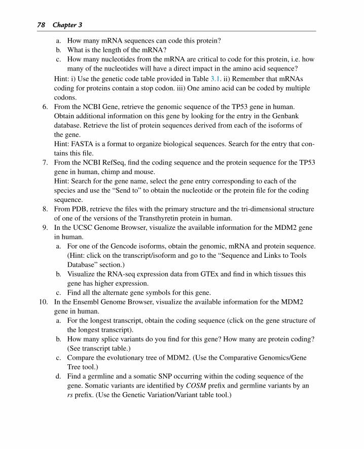
78 Chapter 3

a. How many mRNA sequences can code this protein?b. What is the length of the mRNA?c. How many nucleotides from the mRNA are critical to code for this protein, i.e. how

many of the nucleotides will have a direct impact in the amino acid sequence?

Hint: i) Use the genetic code table provided in Table 3.1. ii) Remember that mRNAscoding for proteins contain a stop codon. iii) One amino acid can be coded by multiplecodons.

6. From the NCBI Gene, retrieve the genomic sequence of the TP53 gene in human.Obtain additional information on this gene by looking for the entry in the Genbankdatabase. Retrieve the list of protein sequences derived from each of the isoforms ofthe gene.Hint: FASTA is a format to organize biological sequences. Search for the entry that con-tains this file.

7. From the NCBI RefSeq, find the coding sequence and the protein sequence for the TP53gene in human, chimp and mouse.Hint: Search for the gene name, select the gene entry corresponding to each of thespecies and use the “Send to” to obtain the nucleotide or the protein file for the codingsequence.

8. From PDB, retrieve the files with the primary structure and the tri-dimensional structureof one of the versions of the Transthyretin protein in human.

9. In the UCSC Genome Browser, visualize the available information for the MDM2 genein human.a. For one of the Gencode isoforms, obtain the genomic, mRNA and protein sequence.

(Hint: click on the transcript/isoform and go to the “Sequence and Links to ToolsDatabase” section.)

b. Visualize the RNA-seq expression data from GTEx and find in which tissues thisgene has higher expression.

c. Find all the alternate gene symbols for this gene.10. In the Ensembl Genome Browser, visualize the available information for the MDM2

gene in human.a. For the longest transcript, obtain the coding sequence (click on the gene structure of

the longest transcript).b. How many splice variants do you find for this gene? How many are protein coding?

(See transcript table.)c. Compare the evolutionary tree of MDM2. (Use the Comparative Genomics/Gene

Tree tool.)d. Find a germline and a somatic SNP occurring within the coding sequence of the

gene. Somatic variants are identified by COSM prefix and germline variants by anrs prefix. (Use the Genetic Variation/Variant table tool.)

CHAPTER 4

Basic Processing of Biological SequencesIn this chapter, we address the computational representation of biological sequences and coverbasic algorithms for their processing. We will address the implementation of the processesrelated to gene expression, covering transcription, translation and the identification of openreading frames. We also cover the implementation of a class for biological sequences (in-cluding DNA, RNA and protein sequences). Finally, we will review a set of classes from theBioPython package to store and process sequences, together with their annotations, allowingtheir loading from databases and reading/writing from files in different formats.

4.1 Biological Sequences: Representations and Basic Algorithms

As previously discussed, in Chapter 3, in biological systems, the genetic information is en-coded into DNA molecules. For many practical purposes, in Bioinformatics algorithms andtools, these molecules can be represented as one-dimensional sequences of nucleotides.

Since in DNA (or RNA) molecules, there are four distinct types of nucleotides, the compu-tational representation of these sequences consists of strings (i.e. sequences of characters)defined over an alphabet of four distinct symbols. For DNA, these symbols are the letters A,C, G, and T, which represent, respectively, adenine, cytosine, guanine and thymine, while, inthe case of RNA, the T gives place to a U, representing uracil.

Although the basic alphabet for DNA only contains the symbols for the four nucleotides, theInternational Union of Pure and Applied Chemistry (IUPAC) has defined an extended set ofsymbols that allow ambiguity in the identification of a nucleotide, useful for instance in theresults of a sequencing process in positions where there is uncertainty in the identificationof the nucleotide, or in the design of Polymerase Chain Reaction (PCR) primers. Table 4.1shows the symbols in this IUPAC alphabet and their meaning.

The other most important biological sequences are proteins, which are typically representedby sequences of aminoacids. In the standard genetic code, there are 20 different encodedaminoacids that can occur in protein sequences, and thus the strings are defined in an alpha-bet of 20 characters (see Table 4.2). In some cases, it is important to add to this alphabet asymbol representing the decoding of a stop codon, to be used for instance when running auto-matic tools for DNA translation, which we will cover in more detail in the next sections. Themost used symbols for the stop codon are the underscore (_) or the asterisk (*).

Bioinformatics Algorithms. DOI: 10.1016/B978-0-12-812520-5.00004-3Copyright © 2018 Elsevier Inc. All rights reserved. 79

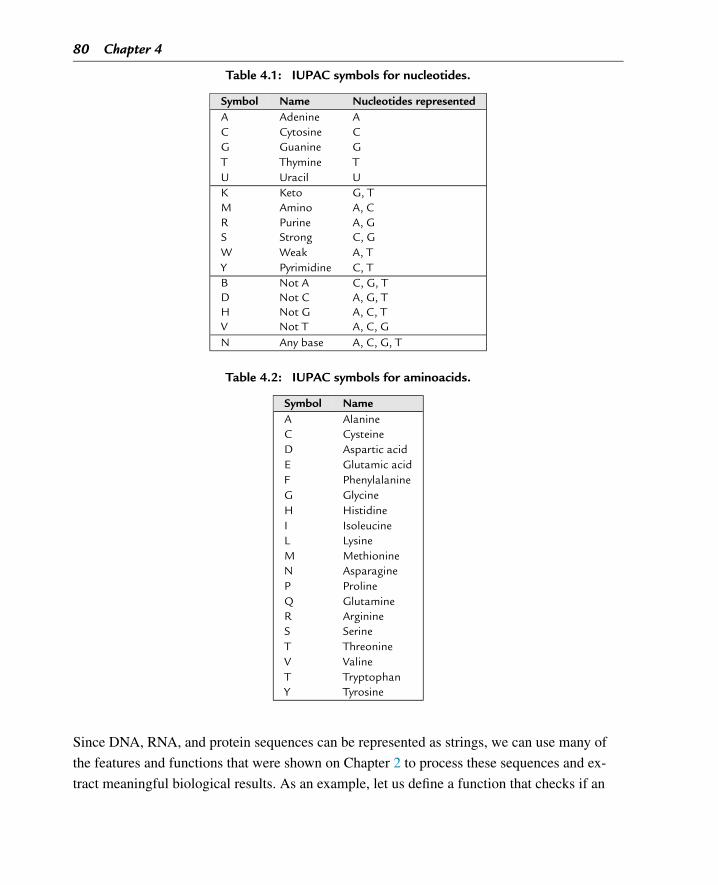
80 Chapter 4

Table 4.1: IUPAC symbols for nucleotides.

Symbol Name Nucleotides representedA Adenine AC Cytosine CG Guanine GT Thymine TU Uracil UK Keto G, TM Amino A, CR Purine A, GS Strong C, GW Weak A, TY Pyrimidine C, TB Not A C, G, TD Not C A, G, TH Not G A, C, TV Not T A, C, GN Any base A, C, G, T

Table 4.2: IUPAC symbols for aminoacids.

Symbol NameA AlanineC CysteineD Aspartic acidE Glutamic acidF PhenylalanineG GlycineH HistidineI IsoleucineL LysineM MethionineN AsparagineP ProlineQ GlutamineR ArginineS SerineT ThreonineV ValineT TryptophanY Tyrosine

Since DNA, RNA, and protein sequences can be represented as strings, we can use many of

the features and functions that were shown on Chapter 2 to process these sequences and ex-

tract meaningful biological results. As an example, let us define a function that checks if an

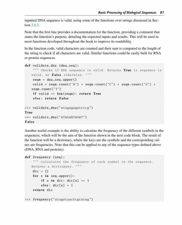
Basic Processing of Biological Sequences 81

inputted DNA sequence is valid, using some of the functions over strings discussed in Sec-tion 2.6.3.

Note that the first line provides a documentation for the function, providing a comment thatstates the function’s purpose, detailing the expected inputs and results. This will be used inmost functions developed throughout the book to improve its readability.

In the function code, valid characters are counted and their sum is compared to the length ofthe string to check if all characters are valid. Similar functions could be easily built for RNAor protein sequences.

def validate_dna (dna_seq):""" Checks if DNA sequence is valid. Returns True is sequence isvalid, or F a l s e otherwise. """seqm = dna_seq.upper()

valid = seqm.count("A") + seqm.count("C") + seqm.count("G") +

seqm.count("T")

i f valid == l e n (seqm): re turn Truee l s e : re turn F a l s e

>>> validate_dna("atagagagatctcg")

True>>> validate_dna("ATAGAXTAGAT")

F a l s e

Another useful example is the ability to calculate the frequency of the different symbols in thesequences, which will be the aim of the function shown in the next code block. The result ofthe function will be a dictionary, where the keys are the symbols and the corresponding val-ues are frequencies. Note that this can be applied to any of the sequence types defined above(DNA, RNA and proteins).

def frequency (seq):""" Calculates the frequency of each symbol in the sequence.

Returns a dictionary. """

dic = {}

f o r s in seq.upper():

i f s in dic: dic[s] += 1

e l s e : dic[s] = 1re turn dic

>>> frequency("atagataactcgcatag")

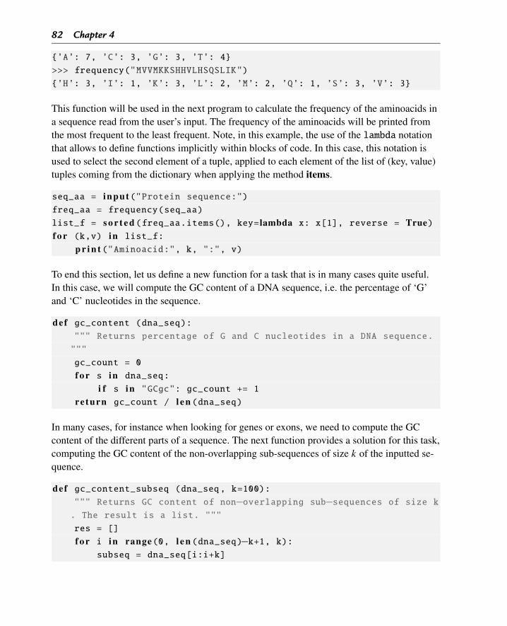
82 Chapter 4

{’A’: 7, ’C’: 3, ’G’: 3, ’T’: 4}

>>> frequency("MVVMKKSHHVLHSQSLIK")

{’H’: 3, ’I’: 1, ’K’: 3, ’L’: 2, ’M’: 2, ’Q’: 1, ’S’: 3, ’V’: 3}

This function will be used in the next program to calculate the frequency of the aminoacids ina sequence read from the user’s input. The frequency of the aminoacids will be printed fromthe most frequent to the least frequent. Note, in this example, the use of the lambda notationthat allows to define functions implicitly within blocks of code. In this case, this notation isused to select the second element of a tuple, applied to each element of the list of (key, value)tuples coming from the dictionary when applying the method items.

seq_aa = input("Protein sequence:")freq_aa = frequency(seq_aa)

list_f = s o r t e d (freq_aa.items(), key= lambda x: x[1], reverse = True)f o r (k,v) in list_f:

p r i n t ("Aminoacid:", k, ":", v)

To end this section, let us define a new function for a task that is in many cases quite useful.In this case, we will compute the GC content of a DNA sequence, i.e. the percentage of ‘G’and ‘C’ nucleotides in the sequence.

def gc_content (dna_seq):""" Returns percentage of G and C nucleotides in a DNA sequence.

"""

gc_count = 0

f o r s in dna_seq:

i f s in "GCgc": gc_count += 1

re turn gc_count / l e n (dna_seq)

In many cases, for instance when looking for genes or exons, we need to compute the GCcontent of the different parts of a sequence. The next function provides a solution for this task,computing the GC content of the non-overlapping sub-sequences of size k of the inputted se-quence.

def gc_content_subseq (dna_seq, k=100):""" Returns GC content of non−overlapping sub−sequences of size k. The result is a list. """

res = []

f o r i in range(0, l e n (dna_seq)−k+1, k):subseq = dna_seq[i:i+k]

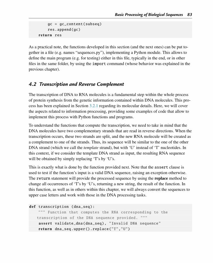
Basic Processing of Biological Sequences 83

gc = gc_content(subseq)

res.append(gc)

re turn res

As a practical note, the functions developed in this section (and the next ones) can be put to-gether in a file (e.g. names “sequences.py”), implementing a Python module. This allows todefine the main program (e.g. for testing) either in this file, typically in the end, or in otherfiles in the same folder, by using the import command (whose behavior was explained in theprevious chapter).

4.2 Transcription and Reverse Complement

The transcription of DNA to RNA molecules is a fundamental step within the whole processof protein synthesis from the genetic information contained within DNA molecules. This pro-cess has been explained in Section 3.2.1 regarding its molecular details. Here, we will coverthe aspects related to information processing, providing some examples of code that allow toimplement this process with Python functions and programs.

To understand the functions that compute the transcription, we need to take in mind that theDNA molecules have two complementary strands that are read in reverse directions. When thetranscription occurs, these two strands are split, and the new RNA molecule will be created asa complement to one of the strands. Thus, its sequence will be similar to the one of the otherDNA strand (which we call the template strand), but with ‘U’ instead of ‘T’ nucleotides. Inthis context, if we consider the template DNA strand as input, the resulting RNA sequencewill be obtained by simply replacing ‘T’s by ‘U’s.

This is exactly what is done by the function provided next. Note that the assert clause isused to test if the function’s input is a valid DNA sequence, raising an exception otherwise.The return statement will provide the processed sequence by using the replace method tochange all occurrences of ‘T’s by ‘U’s, returning a new string, the result of the function. Inthis function, as well as in others within this chapter, we will always convert the sequences toupper case letters and work with those in the DNA processing tasks.

def transcription (dna_seq):""" Function that computes the RNA corresponding to the

transcription of the DNA sequence provided. """

a s s e r t validate_dna(dna_seq), "Invalid DNA sequence"re turn dna_seq.upper().replace("T","U")

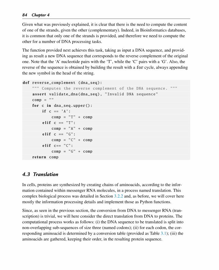
84 Chapter 4

Given what was previously explained, it is clear that there is the need to compute the contentof one of the strands, given the other (complementary). Indeed, in Bioinformatics databases,it is common that only one of the strands is provided, and therefore we need to compute theother for a number of DNA processing tasks.

The function provided next achieves this task, taking as input a DNA sequence, and provid-ing as result a new DNA sequence that corresponds to the reverse complement of the originalone. Note that the ‘A’ nucleotide pairs with the ‘T’, while the ‘C’ pairs with a ‘G’. Also, thereverse of the sequence is obtained by building the result with a for cycle, always appendingthe new symbol in the head of the string.

def reverse_complement (dna_seq):""" Computes the reverse complement of the DNA sequence. """

a s s e r t validate_dna(dna_seq), "Invalid DNA sequence"comp = ""

f o r c in dna_seq.upper():

i f c == ’A’:comp = "T" + comp

e l i f c == "T":comp = "A" + comp

e l i f c == "G":comp = "C" + comp

e l i f c== "C":comp = "G" + comp

re turn comp

4.3 Translation

In cells, proteins are synthesized by creating chains of aminoacids, according to the infor-mation contained within messenger RNA molecules, in a process named translation. Thiscomplex biological process was detailed in Section 3.2.2 and, as before, we will cover heremostly the information processing details and implement those as Python functions.

Since, as seen in the previous section, the conversion from DNA to messenger RNA (tran-scription) is trivial, we will here consider the direct translation from DNA to proteins. Thecomputational process works as follows: (i) the DNA sequence to be translated is split intonon-overlapping sub-sequences of size three (named codons); (ii) for each codon, the cor-responding aminoacid is determined by a conversion table (provided as Table 3.1); (iii) theaminoacids are gathered, keeping their order, in the resulting protein sequence.

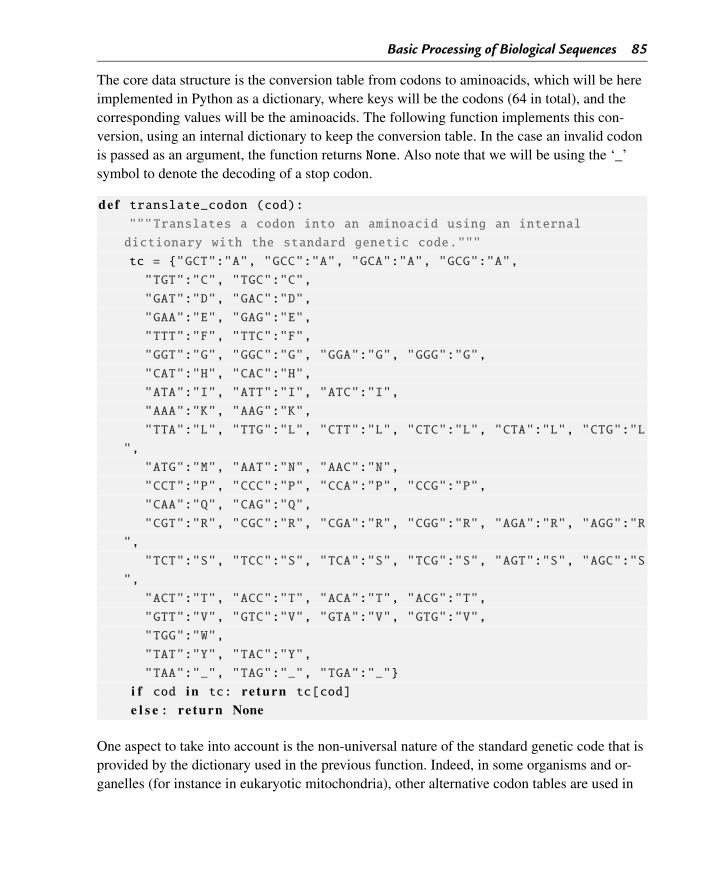
Basic Processing of Biological Sequences 85

The core data structure is the conversion table from codons to aminoacids, which will be hereimplemented in Python as a dictionary, where keys will be the codons (64 in total), and thecorresponding values will be the aminoacids. The following function implements this con-version, using an internal dictionary to keep the conversion table. In the case an invalid codonis passed as an argument, the function returns None. Also note that we will be using the ‘_’symbol to denote the decoding of a stop codon.

def translate_codon (cod):"""Translates a codon into an aminoacid using an internal

dictionary with the standard genetic code."""

tc = {"GCT":"A", "GCC":"A", "GCA":"A", "GCG":"A",

"TGT":"C", "TGC":"C",

"GAT":"D", "GAC":"D",

"GAA":"E", "GAG":"E",

"TTT":"F", "TTC":"F",

"GGT":"G", "GGC":"G", "GGA":"G", "GGG":"G",

"CAT":"H", "CAC":"H",

"ATA":"I", "ATT":"I", "ATC":"I",

"AAA":"K", "AAG":"K",

"TTA":"L", "TTG":"L", "CTT":"L", "CTC":"L", "CTA":"L", "CTG":"L

",

"ATG":"M", "AAT":"N", "AAC":"N",

"CCT":"P", "CCC":"P", "CCA":"P", "CCG":"P",

"CAA":"Q", "CAG":"Q",

"CGT":"R", "CGC":"R", "CGA":"R", "CGG":"R", "AGA":"R", "AGG":"R

",

"TCT":"S", "TCC":"S", "TCA":"S", "TCG":"S", "AGT":"S", "AGC":"S

",

"ACT":"T", "ACC":"T", "ACA":"T", "ACG":"T",

"GTT":"V", "GTC":"V", "GTA":"V", "GTG":"V",

"TGG":"W",

"TAT":"Y", "TAC":"Y",

"TAA":"_", "TAG":"_", "TGA":"_"}

i f cod in tc: re turn tc[cod]

e l s e : re turn None

One aspect to take into account is the non-universal nature of the standard genetic code that isprovided by the dictionary used in the previous function. Indeed, in some organisms and or-ganelles (for instance in eukaryotic mitochondria), other alternative codon tables are used in

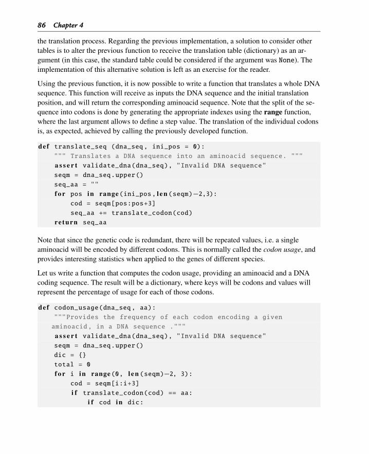
86 Chapter 4

the translation process. Regarding the previous implementation, a solution to consider othertables is to alter the previous function to receive the translation table (dictionary) as an ar-gument (in this case, the standard table could be considered if the argument was None). Theimplementation of this alternative solution is left as an exercise for the reader.

Using the previous function, it is now possible to write a function that translates a whole DNAsequence. This function will receive as inputs the DNA sequence and the initial translationposition, and will return the corresponding aminoacid sequence. Note that the split of the se-quence into codons is done by generating the appropriate indexes using the range function,where the last argument allows to define a step value. The translation of the individual codonsis, as expected, achieved by calling the previously developed function.

def translate_seq (dna_seq, ini_pos = 0):""" Translates a DNA sequence into an aminoacid sequence. """

a s s e r t validate_dna(dna_seq), "Invalid DNA sequence"seqm = dna_seq.upper()

seq_aa = ""

f o r pos in range(ini_pos, l e n (seqm)−2,3):cod = seqm[pos:pos+3]

seq_aa += translate_codon(cod)

re turn seq_aa

Note that since the genetic code is redundant, there will be repeated values, i.e. a singleaminoacid will be encoded by different codons. This is normally called the codon usage, andprovides interesting statistics when applied to the genes of different species.

Let us write a function that computes the codon usage, providing an aminoacid and a DNAcoding sequence. The result will be a dictionary, where keys will be codons and values willrepresent the percentage of usage for each of those codons.

def codon_usage(dna_seq, aa):"""Provides the frequency of each codon encoding a given

aminoacid, in a DNA sequence ."""

a s s e r t validate_dna(dna_seq), "Invalid DNA sequence"seqm = dna_seq.upper()

dic = {}

total = 0

f o r i in range(0, l e n (seqm)−2, 3):cod = seqm[i:i+3]

i f translate_codon(cod) == aa:i f cod in dic:

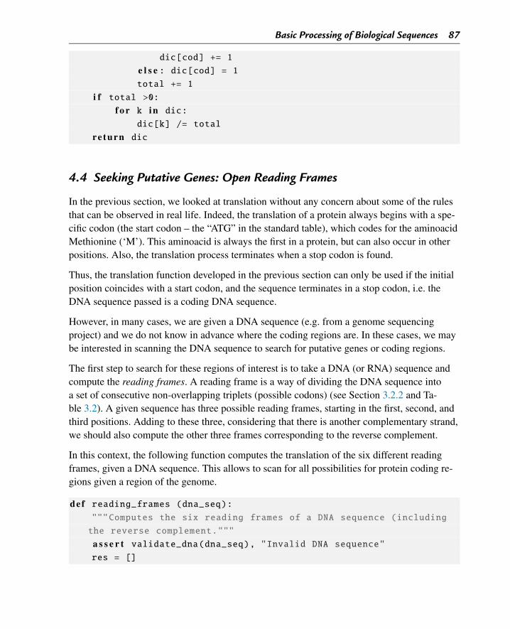
Basic Processing of Biological Sequences 87

dic[cod] += 1

e l s e : dic[cod] = 1total += 1

i f total >0:f o r k in dic:

dic[k] /= total

re turn dic

4.4 Seeking Putative Genes: Open Reading Frames

In the previous section, we looked at translation without any concern about some of the rulesthat can be observed in real life. Indeed, the translation of a protein always begins with a spe-cific codon (the start codon – the “ATG” in the standard table), which codes for the aminoacidMethionine (‘M’). This aminoacid is always the first in a protein, but can also occur in otherpositions. Also, the translation process terminates when a stop codon is found.

Thus, the translation function developed in the previous section can only be used if the initialposition coincides with a start codon, and the sequence terminates in a stop codon, i.e. theDNA sequence passed is a coding DNA sequence.

However, in many cases, we are given a DNA sequence (e.g. from a genome sequencingproject) and we do not know in advance where the coding regions are. In these cases, we maybe interested in scanning the DNA sequence to search for putative genes or coding regions.

The first step to search for these regions of interest is to take a DNA (or RNA) sequence andcompute the reading frames. A reading frame is a way of dividing the DNA sequence intoa set of consecutive non-overlapping triplets (possible codons) (see Section 3.2.2 and Ta-ble 3.2). A given sequence has three possible reading frames, starting in the first, second, andthird positions. Adding to these three, considering that there is another complementary strand,we should also compute the other three frames corresponding to the reverse complement.

In this context, the following function computes the translation of the six different readingframes, given a DNA sequence. This allows to scan for all possibilities for protein coding re-gions given a region of the genome.

def reading_frames (dna_seq):"""Computes the six reading frames of a DNA sequence (including

the reverse complement."""

a s s e r t validate_dna(dna_seq), "Invalid DNA sequence"res = []

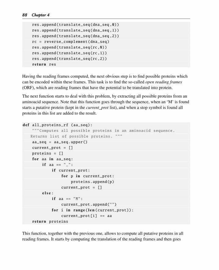
88 Chapter 4

res.append(translate_seq(dna_seq ,0))

res.append(translate_seq(dna_seq ,1))

res.append(translate_seq(dna_seq ,2))

rc = reverse_complement(dna_seq)

res.append(translate_seq(rc,0))

res.append(translate_seq(rc,1))

res.append(translate_seq(rc,2))

re turn res

Having the reading frames computed, the next obvious step is to find possible proteins whichcan be encoded within these frames. This task is to find the so-called open reading frames(ORF), which are reading frames that have the potential to be translated into protein.

The next function starts to deal with this problem, by extracting all possible proteins from anaminoacid sequence. Note that this function goes through the sequence, when an ‘M’ is foundstarts a putative protein (kept in the current_prot list), and when a stop symbol is found allproteins in this list are added to the result.

def all_proteins_rf (aa_seq):"""Computes all possible proteins in an aminoacid sequence.

Returns list of possible proteins. """

aa_seq = aa_seq.upper()

current_prot = []

proteins = []

f o r aa in aa_seq:

i f aa == "_":i f current_prot:

f o r p in current_prot:

proteins.append(p)

current_prot = []

e l s e :i f aa == "M":

current_prot.append("")

f o r i in range( l e n (current_prot)):current_prot[i] += aa

re turn proteins

This function, together with the previous one, allows to compute all putative proteins in allreading frames. It starts by computing the translation of the reading frames and then goes

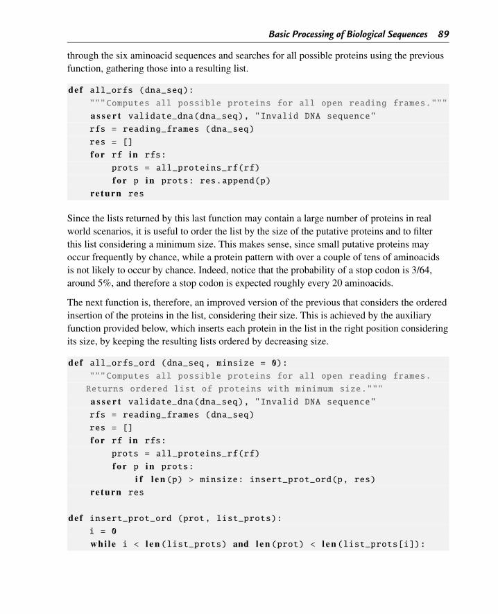
Basic Processing of Biological Sequences 89

through the six aminoacid sequences and searches for all possible proteins using the previousfunction, gathering those into a resulting list.

def all_orfs (dna_seq):"""Computes all possible proteins for all open reading frames."""

a s s e r t validate_dna(dna_seq), "Invalid DNA sequence"rfs = reading_frames (dna_seq)

res = []

f o r rf in rfs:

prots = all_proteins_rf(rf)

f o r p in prots: res.append(p)

re turn res

Since the lists returned by this last function may contain a large number of proteins in realworld scenarios, it is useful to order the list by the size of the putative proteins and to filterthis list considering a minimum size. This makes sense, since small putative proteins mayoccur frequently by chance, while a protein pattern with over a couple of tens of aminoacidsis not likely to occur by chance. Indeed, notice that the probability of a stop codon is 3/64,around 5%, and therefore a stop codon is expected roughly every 20 aminoacids.

The next function is, therefore, an improved version of the previous that considers the orderedinsertion of the proteins in the list, considering their size. This is achieved by the auxiliaryfunction provided below, which inserts each protein in the list in the right position consideringits size, by keeping the resulting lists ordered by decreasing size.

def all_orfs_ord (dna_seq, minsize = 0):"""Computes all possible proteins for all open reading frames.

Returns ordered list of proteins with minimum size."""

a s s e r t validate_dna(dna_seq), "Invalid DNA sequence"rfs = reading_frames (dna_seq)

res = []

f o r rf in rfs:

prots = all_proteins_rf(rf)

f o r p in prots:

i f l e n (p) > minsize: insert_prot_ord(p, res)re turn res

def insert_prot_ord (prot, list_prots):i = 0

whi le i < l e n (list_prots) and l e n (prot) < l e n (list_prots[i]):

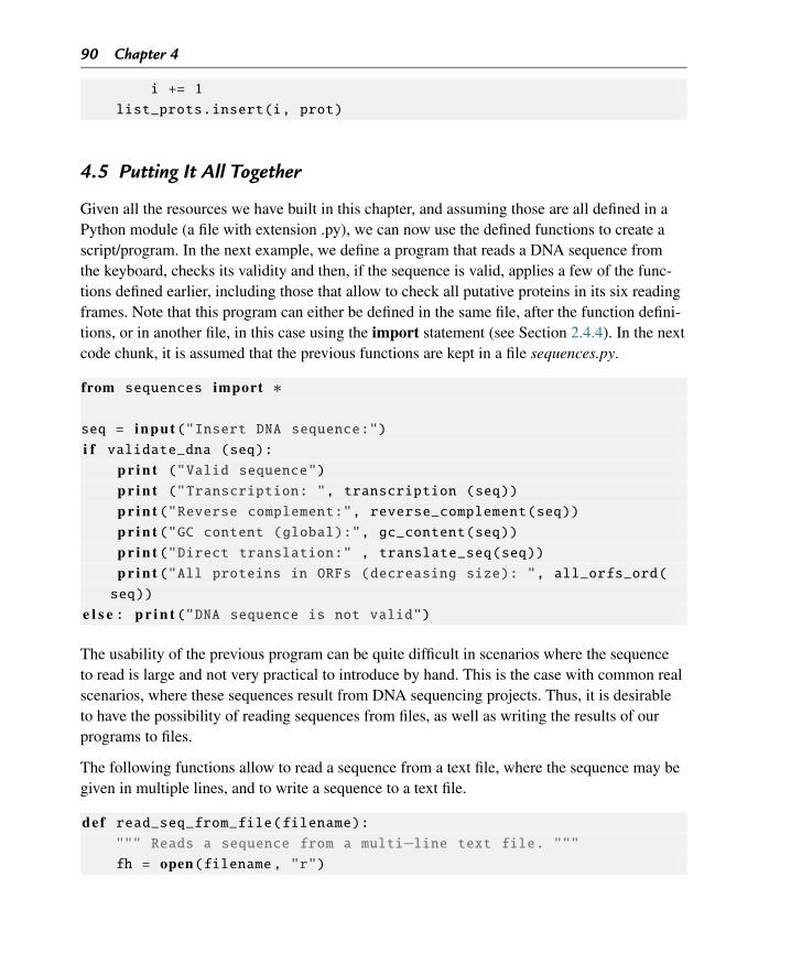
90 Chapter 4

i += 1

list_prots.insert(i, prot)

4.5 Putting It All Together

Given all the resources we have built in this chapter, and assuming those are all defined in aPython module (a file with extension .py), we can now use the defined functions to create ascript/program. In the next example, we define a program that reads a DNA sequence fromthe keyboard, checks its validity and then, if the sequence is valid, applies a few of the func-tions defined earlier, including those that allow to check all putative proteins in its six readingframes. Note that this program can either be defined in the same file, after the function defini-tions, or in another file, in this case using the import statement (see Section 2.4.4). In the nextcode chunk, it is assumed that the previous functions are kept in a file sequences.py.

from sequences import ∗

seq = input("Insert DNA sequence:")i f validate_dna (seq):

p r i n t ("Valid sequence")p r i n t ("Transcription: ", transcription (seq))p r i n t ("Reverse complement:", reverse_complement(seq))p r i n t ("GC content (global):", gc_content(seq))p r i n t ("Direct translation:" , translate_seq(seq))p r i n t ("All proteins in ORFs (decreasing size): ", all_orfs_ord(seq))

e l s e : p r i n t ("DNA sequence is not valid")

The usability of the previous program can be quite difficult in scenarios where the sequenceto read is large and not very practical to introduce by hand. This is the case with common realscenarios, where these sequences result from DNA sequencing projects. Thus, it is desirableto have the possibility of reading sequences from files, as well as writing the results of ourprograms to files.

The following functions allow to read a sequence from a text file, where the sequence may begiven in multiple lines, and to write a sequence to a text file.

def read_seq_from_file(filename):""" Reads a sequence from a multi−line text file. """fh = open(filename, "r")

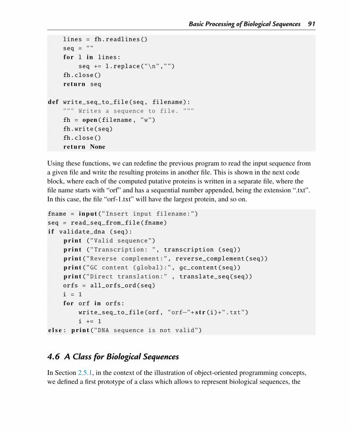
Basic Processing of Biological Sequences 91

lines = fh.readlines()

seq = ""

f o r l in lines:

seq += l.replace("\n","")

fh.close()

re turn seq

def write_seq_to_file(seq, filename):""" Writes a sequence to file. """

fh = open(filename, "w")fh.write(seq)

fh.close()

re turn None

Using these functions, we can redefine the previous program to read the input sequence froma given file and write the resulting proteins in another file. This is shown in the next codeblock, where each of the computed putative proteins is written in a separate file, where thefile name starts with “orf” and has a sequential number appended, being the extension “.txt”.In this case, the file “orf-1.txt” will have the largest protein, and so on.

fname = input("Insert input filename:")seq = read_seq_from_file(fname)

i f validate_dna (seq):p r i n t ("Valid sequence")p r i n t ("Transcription: ", transcription (seq))p r i n t ("Reverse complement:", reverse_complement(seq))p r i n t ("GC content (global):", gc_content(seq))p r i n t ("Direct translation:" , translate_seq(seq))orfs = all_orfs_ord(seq)

i = 1

f o r orf in orfs:

write_seq_to_file(orf, "orf−"+ s t r (i)+".txt")i += 1

e l s e : p r i n t ("DNA sequence is not valid")

4.6 A Class for Biological Sequences

In Section 2.5.1, in the context of the illustration of object-oriented programming concepts,we defined a first prototype of a class which allows to represent biological sequences, the

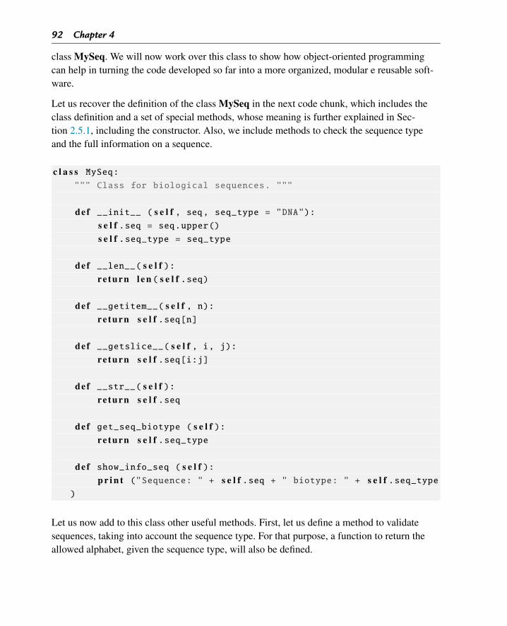
92 Chapter 4

class MySeq. We will now work over this class to show how object-oriented programmingcan help in turning the code developed so far into a more organized, modular e reusable soft-ware.

Let us recover the definition of the class MySeq in the next code chunk, which includes theclass definition and a set of special methods, whose meaning is further explained in Sec-tion 2.5.1, including the constructor. Also, we include methods to check the sequence typeand the full information on a sequence.

c l a s s MySeq:""" Class for biological sequences. """

def __init__ ( s e l f , seq, seq_type = "DNA"):s e l f .seq = seq.upper()s e l f .seq_type = seq_type

def __len__( s e l f ):re turn l e n ( s e l f .seq)

def __getitem__( s e l f , n):re turn s e l f .seq[n]

def __getslice__( s e l f , i, j):re turn s e l f .seq[i:j]

def __str__( s e l f ):re turn s e l f .seq

def get_seq_biotype ( s e l f ):re turn s e l f .seq_type

def show_info_seq ( s e l f ):p r i n t ("Sequence: " + s e l f .seq + " biotype: " + s e l f .seq_type

)

Let us now add to this class other useful methods. First, let us define a method to validatesequences, taking into account the sequence type. For that purpose, a function to return theallowed alphabet, given the sequence type, will also be defined.

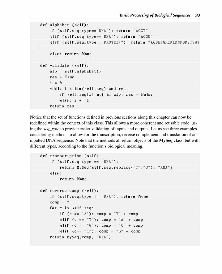
Basic Processing of Biological Sequences 93

def alphabet ( s e l f ):i f ( s e l f .seq_type=="DNA"): re turn "ACGT"e l i f ( s e l f .seq_type=="RNA"): re turn "ACGU"e l i f ( s e l f .seq_type=="PROTEIN"): re turn "ACDEFGHIKLMNPQRSTVWY

"

e l s e : re turn None

def validate ( s e l f ):alp = s e l f .alphabet()res = Truei = 0

whi le i < l e n ( s e l f .seq) and res:i f s e l f .seq[i] not in alp: res = F a l s ee l s e : i += 1

re turn res

Notice that the set of functions defined in previous sections along this chapter can now beredefined within the context of this class. This allows a more coherent and reusable code, us-ing the seq_type to provide easier validation of inputs and outputs. Let us see three examplesconsidering methods to allow for the transcription, reverse complement and translation of aninputted DNA sequence. Note that the methods all return objects of the MySeq class, but withdifferent types, according to the function’s biological meaning.

def transcription ( s e l f ):i f ( s e l f .seq_type == "DNA"):

re turn MySeq( s e l f .seq.replace("T","U"), "RNA")e l s e :

re turn None

def reverse_comp ( s e l f ):i f ( s e l f .seq_type != "DNA"): re turn Nonecomp = ""

f o r c in s e l f .seq:i f (c == ’A’): comp = "T" + compe l i f (c == "T"): comp = "A" + compe l i f (c == "G"): comp = "C" + compe l i f (c== "C"): comp = "G" + comp

re turn MySeq(comp, "DNA")

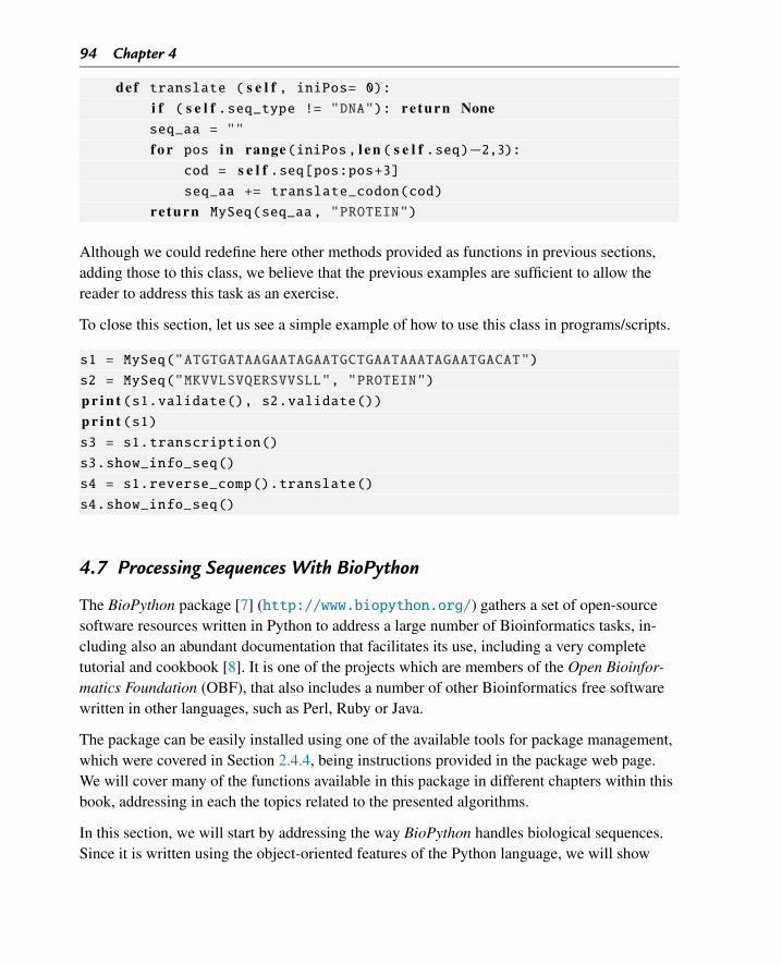
94 Chapter 4

def translate ( s e l f , iniPos= 0):i f ( s e l f .seq_type != "DNA"): re turn Noneseq_aa = ""

f o r pos in range(iniPos, l e n ( s e l f .seq)−2,3):cod = s e l f .seq[pos:pos+3]seq_aa += translate_codon(cod)

re turn MySeq(seq_aa, "PROTEIN")

Although we could redefine here other methods provided as functions in previous sections,adding those to this class, we believe that the previous examples are sufficient to allow thereader to address this task as an exercise.

To close this section, let us see a simple example of how to use this class in programs/scripts.

s1 = MySeq("ATGTGATAAGAATAGAATGCTGAATAAATAGAATGACAT")

s2 = MySeq("MKVVLSVQERSVVSLL", "PROTEIN")

p r i n t (s1.validate(), s2.validate())p r i n t (s1)s3 = s1.transcription()

s3.show_info_seq()

s4 = s1.reverse_comp().translate()

s4.show_info_seq()

4.7 Processing Sequences With BioPython

The BioPython package [7] (http://www.biopython.org/) gathers a set of open-sourcesoftware resources written in Python to address a large number of Bioinformatics tasks, in-cluding also an abundant documentation that facilitates its use, including a very completetutorial and cookbook [8]. It is one of the projects which are members of the Open Bioinfor-matics Foundation (OBF), that also includes a number of other Bioinformatics free softwarewritten in other languages, such as Perl, Ruby or Java.

The package can be easily installed using one of the available tools for package management,which were covered in Section 2.4.4, being instructions provided in the package web page.We will cover many of the functions available in this package in different chapters within thisbook, addressing in each the topics related to the presented algorithms.

In this section, we will start by addressing the way BioPython handles biological sequences.Since it is written using the object-oriented features of the Python language, we will show

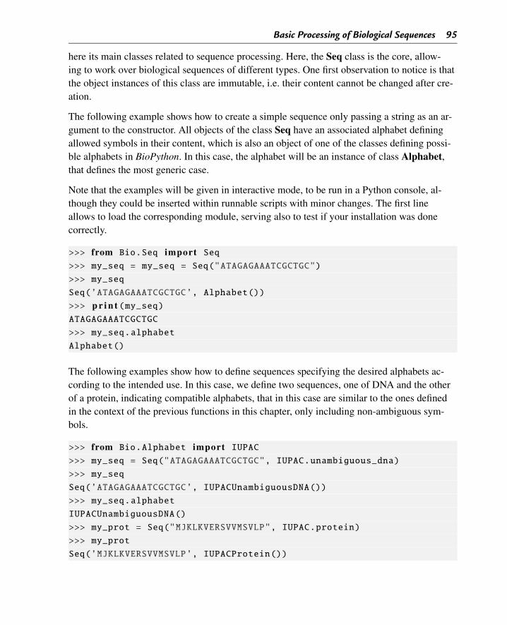
Basic Processing of Biological Sequences 95

here its main classes related to sequence processing. Here, the Seq class is the core, allow-ing to work over biological sequences of different types. One first observation to notice is thatthe object instances of this class are immutable, i.e. their content cannot be changed after cre-ation.

The following example shows how to create a simple sequence only passing a string as an ar-gument to the constructor. All objects of the class Seq have an associated alphabet definingallowed symbols in their content, which is also an object of one of the classes defining possi-ble alphabets in BioPython. In this case, the alphabet will be an instance of class Alphabet,that defines the most generic case.

Note that the examples will be given in interactive mode, to be run in a Python console, al-though they could be inserted within runnable scripts with minor changes. The first lineallows to load the corresponding module, serving also to test if your installation was donecorrectly.

>>> from Bio.Seq import Seq>>> my_seq = my_seq = Seq("ATAGAGAAATCGCTGC")

>>> my_seq

Seq(’ATAGAGAAATCGCTGC’, Alphabet())

>>> p r i n t (my_seq)ATAGAGAAATCGCTGC

>>> my_seq.alphabet

Alphabet()

The following examples show how to define sequences specifying the desired alphabets ac-cording to the intended use. In this case, we define two sequences, one of DNA and the otherof a protein, indicating compatible alphabets, that in this case are similar to the ones definedin the context of the previous functions in this chapter, only including non-ambiguous sym-bols.

>>> from Bio.Alphabet import IUPAC>>> my_seq = Seq("ATAGAGAAATCGCTGC", IUPAC.unambiguous_dna)

>>> my_seq

Seq(’ATAGAGAAATCGCTGC’, IUPACUnambiguousDNA())

>>> my_seq.alphabet

IUPACUnambiguousDNA()

>>> my_prot = Seq("MJKLKVERSVVMSVLP", IUPAC.protein)

>>> my_prot

Seq(’MJKLKVERSVVMSVLP’, IUPACProtein())

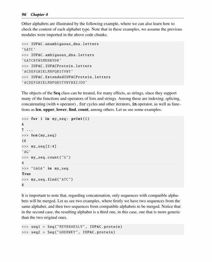
96 Chapter 4

Other alphabets are illustrated by the following example, where we can also learn how tocheck the content of each alphabet type. Note that in these examples, we assume the previousmodules were imported in the above code chunks.

>>> IUPAC.unambiguous_dna.letters

’GATC’

>>> IUPAC.ambiguous_dna.letters

’GATCRYWSMKHBVDN’

>>> IUPAC.IUPACProtein.letters

’ACDEFGHIKLMNPQRSTVWY’

>>> IUPAC.ExtendedIUPACProtein.letters

’ACDEFGHIKLMNPQRSTVWYBXZJUO’

The objects of the Seq class can be treated, for many effects, as strings, since they supportmany of the functions and operators of lists and strings. Among these are indexing, splicing,concatenating (with + operator) , for cycles and other iterators, in operator, as well as func-tions as len, upper, lower, find, count, among others. Let us see some examples:

>>> f o r i in my_seq: p r i n t (i)A

T ...

>>> l e n (my_seq)16

>>> my_seq[2:4]

’AG’

>>> my_seq.count("G")

4

>>> "GAGA" in my_seq

True>>> my_seq.find("ATC")

8

It is important to note that, regarding concatenation, only sequences with compatible alpha-bets will be merged. Let us see two examples, where firstly we have two sequences from thesame alphabet, and then two sequences from compatible alphabets to be merged. Notice thatin the second case, the resulting alphabet is a third one, in this case, one that is more genericthan the two original ones.

>>> seq1 = Seq("MEVRNAKSLV", IUPAC.protein)

>>> seq2 = Seq("GHERWKY", IUPAC.protein)

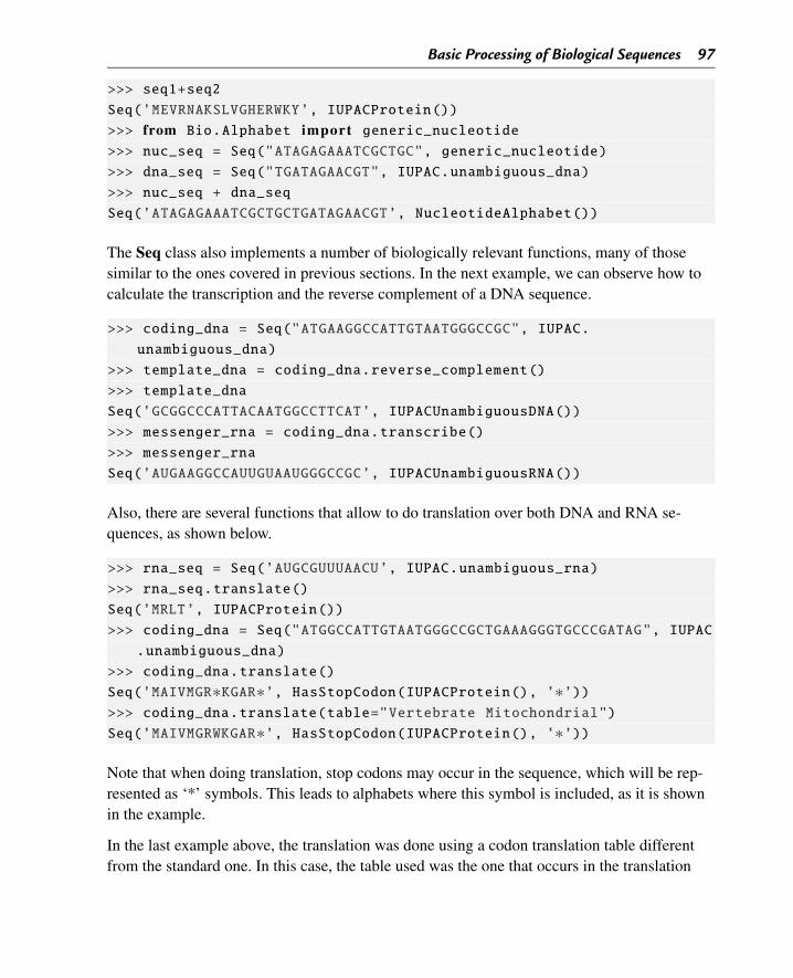
Basic Processing of Biological Sequences 97

>>> seq1+seq2

Seq(’MEVRNAKSLVGHERWKY’, IUPACProtein())

>>> from Bio.Alphabet import generic_nucleotide>>> nuc_seq = Seq("ATAGAGAAATCGCTGC", generic_nucleotide)

>>> dna_seq = Seq("TGATAGAACGT", IUPAC.unambiguous_dna)

>>> nuc_seq + dna_seq

Seq(’ATAGAGAAATCGCTGCTGATAGAACGT’, NucleotideAlphabet())

The Seq class also implements a number of biologically relevant functions, many of thosesimilar to the ones covered in previous sections. In the next example, we can observe how tocalculate the transcription and the reverse complement of a DNA sequence.

>>> coding_dna = Seq("ATGAAGGCCATTGTAATGGGCCGC", IUPAC.

unambiguous_dna)

>>> template_dna = coding_dna.reverse_complement()

>>> template_dna

Seq(’GCGGCCCATTACAATGGCCTTCAT’, IUPACUnambiguousDNA())

>>> messenger_rna = coding_dna.transcribe()

>>> messenger_rna

Seq(’AUGAAGGCCAUUGUAAUGGGCCGC’, IUPACUnambiguousRNA())

Also, there are several functions that allow to do translation over both DNA and RNA se-quences, as shown below.

>>> rna_seq = Seq(’AUGCGUUUAACU’, IUPAC.unambiguous_rna)

>>> rna_seq.translate()

Seq(’MRLT’, IUPACProtein())

>>> coding_dna = Seq("ATGGCCATTGTAATGGGCCGCTGAAAGGGTGCCCGATAG", IUPAC

.unambiguous_dna)

>>> coding_dna.translate()

Seq(’MAIVMGR∗KGAR∗’, HasStopCodon(IUPACProtein(), ’∗’))>>> coding_dna.translate(table="Vertebrate Mitochondrial")

Seq(’MAIVMGRWKGAR∗’, HasStopCodon(IUPACProtein(), ’∗’))

Note that when doing translation, stop codons may occur in the sequence, which will be rep-resented as ‘*’ symbols. This leads to alphabets where this symbol is included, as it is shownin the example.

In the last example above, the translation was done using a codon translation table differentfrom the standard one. In this case, the table used was the one that occurs in the translation

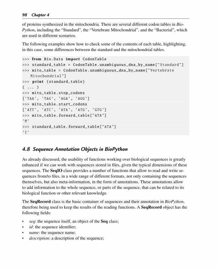
98 Chapter 4

of proteins synthesized in the mitochondria. There are several different codon tables in Bio-Python, including the “Standard”, the “Vertebrate Mitochondrial”, and the “Bacterial”, whichare used in different scenarios.

The following examples show how to check some of the contents of each table, highlighting,in this case, some differences between the standard and the mitochondrial tables.

>>> from Bio.Data import CodonTable>>> standard_table = CodonTable.unambiguous_dna_by_name["Standard"]

>>> mito_table = CodonTable.unambiguous_dna_by_name["Vertebrate

Mitochondrial"]

>>> p r i n t (standard_table)( ... )

>>> mito_table.stop_codons

[’TAA’, ’TAG’, ’AGA’, ’AGG’]

>>> mito_table.start_codons

[’ATT’, ’ATC’, ’ATA’, ’ATG’, ’GTG’]

>>> mito_table.forward_table["ATA"]

’M’

>>> standard_table.forward_table["ATA"]

’I’

4.8 Sequence Annotation Objects in BioPython

As already discussed, the usability of functions working over biological sequences is greatlyenhanced if we can work with sequences stored in files, given the typical dimensions of thesesequences. The SeqIO class provides a number of functions that allow to read and write se-quences from/to files, in a wide range of different formats, not only containing the sequencesthemselves, but also meta-information, in the form of annotations. These annotations allowto add information to the whole sequence, or parts of the sequence, that can be related to itsbiological function or other relevant knowledge.

The SeqRecord class is the basic container of sequences and their annotation in BioPython,therefore being used to keep the results of the reading functions. A SeqRecord object has thefollowing fields:

• seq: the sequence itself, an object of the Seq class;• id: the sequence identifier;• name: the sequence name;• description: a description of the sequence;

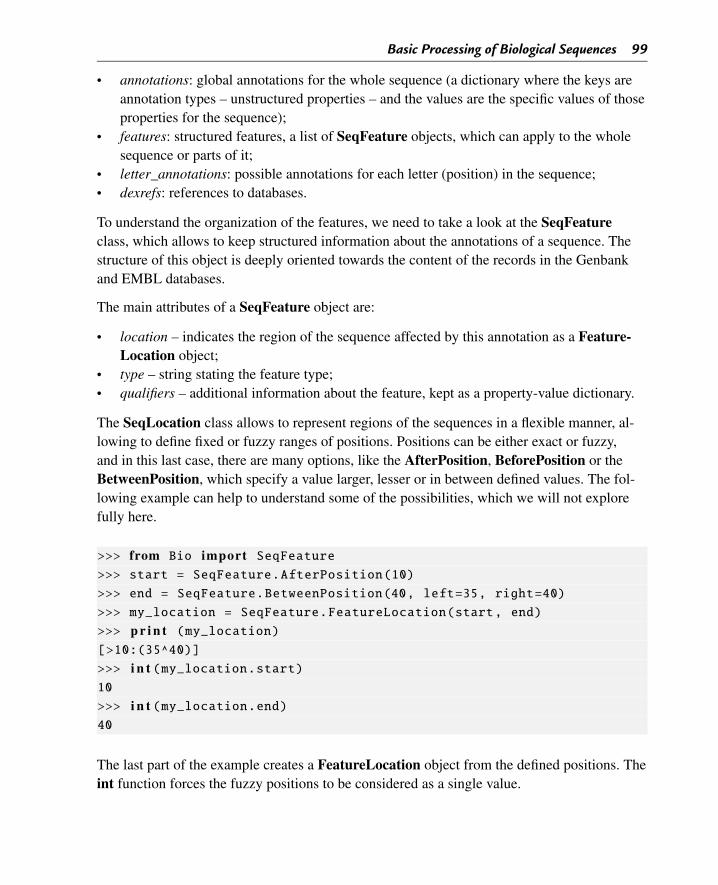
Basic Processing of Biological Sequences 99

• annotations: global annotations for the whole sequence (a dictionary where the keys areannotation types – unstructured properties – and the values are the specific values of thoseproperties for the sequence);

• features: structured features, a list of SeqFeature objects, which can apply to the wholesequence or parts of it;

• letter_annotations: possible annotations for each letter (position) in the sequence;• dexrefs: references to databases.

To understand the organization of the features, we need to take a look at the SeqFeatureclass, which allows to keep structured information about the annotations of a sequence. Thestructure of this object is deeply oriented towards the content of the records in the Genbankand EMBL databases.

The main attributes of a SeqFeature object are:

• location – indicates the region of the sequence affected by this annotation as a Feature-Location object;

• type – string stating the feature type;• qualifiers – additional information about the feature, kept as a property-value dictionary.

The SeqLocation class allows to represent regions of the sequences in a flexible manner, al-lowing to define fixed or fuzzy ranges of positions. Positions can be either exact or fuzzy,and in this last case, there are many options, like the AfterPosition, BeforePosition or theBetweenPosition, which specify a value larger, lesser or in between defined values. The fol-lowing example can help to understand some of the possibilities, which we will not explorefully here.

>>> from Bio import SeqFeature>>> start = SeqFeature.AfterPosition(10)

>>> end = SeqFeature.BetweenPosition(40, left=35, right=40)

>>> my_location = SeqFeature.FeatureLocation(start, end)

>>> p r i n t (my_location)[>10:(35^40)]

>>> i n t (my_location.start)10

>>> i n t (my_location.end)40

The last part of the example creates a FeatureLocation object from the defined positions. Theint function forces the fuzzy positions to be considered as a single value.

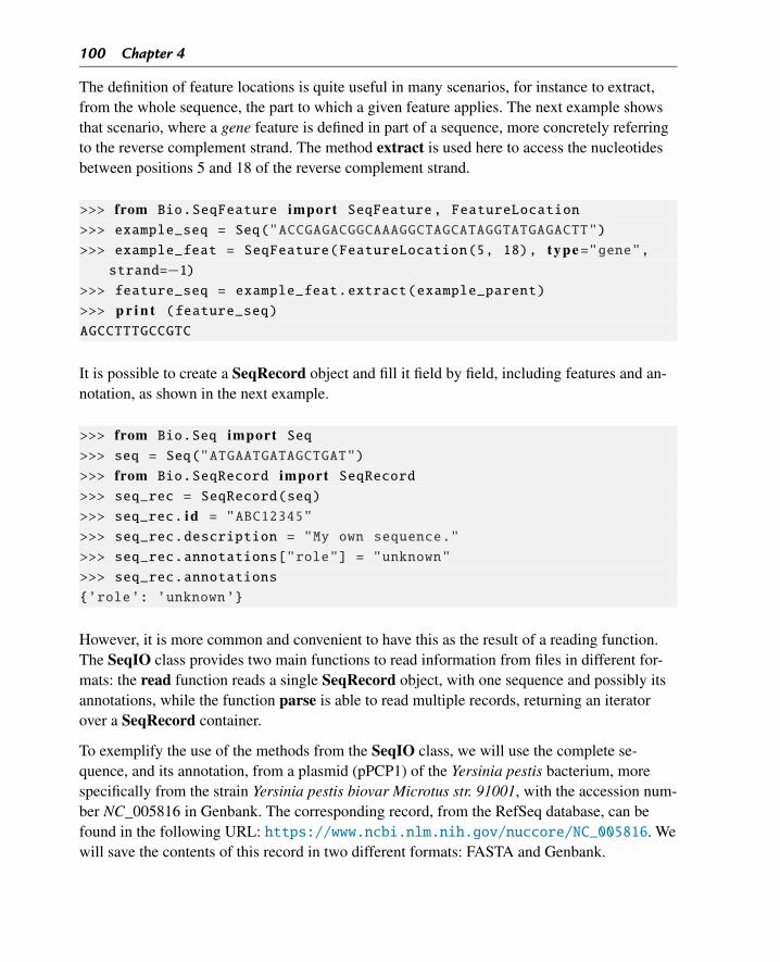
100 Chapter 4

The definition of feature locations is quite useful in many scenarios, for instance to extract,from the whole sequence, the part to which a given feature applies. The next example showsthat scenario, where a gene feature is defined in part of a sequence, more concretely referringto the reverse complement strand. The method extract is used here to access the nucleotidesbetween positions 5 and 18 of the reverse complement strand.

>>> from Bio.SeqFeature import SeqFeature, FeatureLocation>>> example_seq = Seq("ACCGAGACGGCAAAGGCTAGCATAGGTATGAGACTT")

>>> example_feat = SeqFeature(FeatureLocation(5, 18), type="gene",strand=−1)

>>> feature_seq = example_feat.extract(example_parent)

>>> p r i n t (feature_seq)AGCCTTTGCCGTC

It is possible to create a SeqRecord object and fill it field by field, including features and an-notation, as shown in the next example.

>>> from Bio.Seq import Seq>>> seq = Seq("ATGAATGATAGCTGAT")

>>> from Bio.SeqRecord import SeqRecord>>> seq_rec = SeqRecord(seq)

>>> seq_rec. id = "ABC12345"

>>> seq_rec.description = "My own sequence."

>>> seq_rec.annotations["role"] = "unknown"

>>> seq_rec.annotations

{’role’: ’unknown’}

However, it is more common and convenient to have this as the result of a reading function.The SeqIO class provides two main functions to read information from files in different for-mats: the read function reads a single SeqRecord object, with one sequence and possibly itsannotations, while the function parse is able to read multiple records, returning an iteratorover a SeqRecord container.

To exemplify the use of the methods from the SeqIO class, we will use the complete se-quence, and its annotation, from a plasmid (pPCP1) of the Yersinia pestis bacterium, morespecifically from the strain Yersinia pestis biovar Microtus str. 91001, with the accession num-ber NC_005816 in Genbank. The corresponding record, from the RefSeq database, can befound in the following URL: https://www.ncbi.nlm.nih.gov/nuccore/NC_005816. Wewill save the contents of this record in two different formats: FASTA and Genbank.

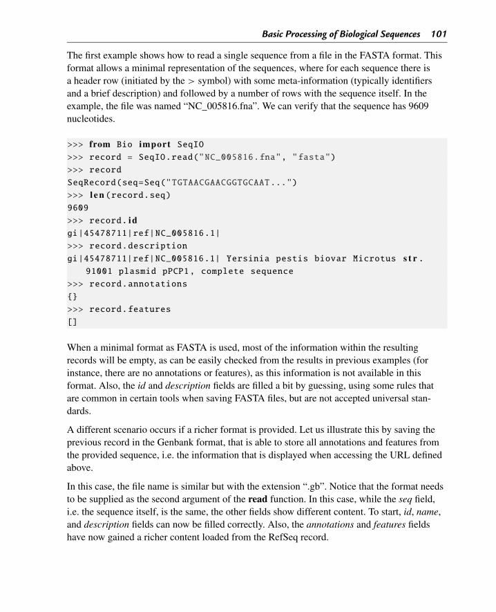
Basic Processing of Biological Sequences 101

The first example shows how to read a single sequence from a file in the FASTA format. Thisformat allows a minimal representation of the sequences, where for each sequence there isa header row (initiated by the > symbol) with some meta-information (typically identifiersand a brief description) and followed by a number of rows with the sequence itself. In theexample, the file was named “NC_005816.fna”. We can verify that the sequence has 9609nucleotides.

>>> from Bio import SeqIO>>> record = SeqIO.read("NC_005816.fna", "fasta")

>>> record

SeqRecord(seq=Seq("TGTAACGAACGGTGCAAT...")

>>> l e n (record.seq)9609

>>> record. idgi|45478711|ref|NC_005816.1|

>>> record.description

gi|45478711|ref|NC_005816.1| Yersinia pestis biovar Microtus s t r .91001 plasmid pPCP1, complete sequence

>>> record.annotations

{}

>>> record.features

[]

When a minimal format as FASTA is used, most of the information within the resultingrecords will be empty, as can be easily checked from the results in previous examples (forinstance, there are no annotations or features), as this information is not available in thisformat. Also, the id and description fields are filled a bit by guessing, using some rules thatare common in certain tools when saving FASTA files, but are not accepted universal stan-dards.

A different scenario occurs if a richer format is provided. Let us illustrate this by saving theprevious record in the Genbank format, that is able to store all annotations and features fromthe provided sequence, i.e. the information that is displayed when accessing the URL definedabove.

In this case, the file name is similar but with the extension “.gb”. Notice that the format needsto be supplied as the second argument of the read function. In this case, while the seq field,i.e. the sequence itself, is the same, the other fields show different content. To start, id, name,and description fields can now be filled correctly. Also, the annotations and features fieldshave now gained a richer content loaded from the RefSeq record.

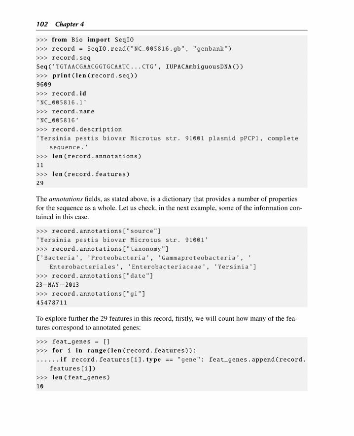
102 Chapter 4

>>> from Bio import SeqIO>>> record = SeqIO.read("NC_005816.gb", "genbank")

>>> record.seq

Seq(’TGTAACGAACGGTGCAATC...CTG’, IUPACAmbiguousDNA())

>>> p r i n t ( l e n (record.seq))9609

>>> record. id’NC_005816.1’

>>> record.name

’NC_005816’

>>> record.description

’Yersinia pestis biovar Microtus str. 91001 plasmid pPCP1, complete

sequence.’

>>> l e n (record.annotations)11

>>> l e n (record.features)29

The annotations fields, as stated above, is a dictionary that provides a number of propertiesfor the sequence as a whole. Let us check, in the next example, some of the information con-tained in this case.

>>> record.annotations["source"]

’Yersinia pestis biovar Microtus str. 91001’

>>> record.annotations["taxonomy"]

[’Bacteria’, ’Proteobacteria’, ’Gammaproteobacteria’, ’

Enterobacteriales’, ’Enterobacteriaceae’, ’Yersinia’]

>>> record.annotations["date"]

23−MAY−2013>>> record.annotations["gi"]

45478711

To explore further the 29 features in this record, firstly, we will count how many of the fea-tures correspond to annotated genes:

>>> feat_genes = []

>>> f o r i in range( l e n (record.features)):...... i f record.features[i]. type == "gene": feat_genes.append(record.

features[i])

>>> l e n (feat_genes)10

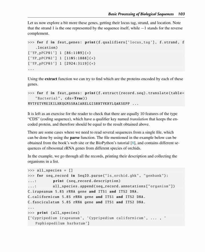
Basic Processing of Biological Sequences 103

Let us now explore a bit more these genes, getting their locus tag, strand, and location. Notethat the strand 1 is the one represented by the sequence itself, while −1 stands for the reversecomplement.

>>> f o r f in feat_genes: p r i n t (f.qualifiers[’locus_tag’], f.strand, f.location)

[’YP_pPCP01’] 1 [86:1109](+)

[’YP_pPCP02’] 1 [1105:1888](+)

[’YP_pPCP03’] 1 [2924:3119](+)

...

Using the extract function we can try to find which are the proteins encoded by each of thesegenes.

>>> f o r f in feat_genes: p r i n t (f.extract(record.seq).translate(table="Bacterial", cds=True))

MVTFETVMEIKILHKQGMSSRAIARELGISRNTVKRYLQAKSEPP ...

It is left as an exercise for the reader to check that there are equally 10 features of the type“CDS” (coding sequence), which have a qualifier key named translation that keeps the en-coded protein, and therefore should be equal to the result obtained above.

There are some cases where we need to read several sequences from a single file, whichcan be done by using the parse function. The file mentioned in the example below can beobtained from the book’s web site or the BioPython’s tutorial [8], and contains different se-quences of ribosomal rRNA genes from different species of orchids.

In the example, we go through all the records, printing their description and collecting theorganisms in a list.

>>> all_species = []

>>> f o r seq_record in SeqIO.parse("ls_orchid.gbk", "genbank"):

...: p r i n t (seq_record.description)

...: all_species.append(seq_record.annotations["organism"])

C.irapeanum 5.8S rRNA gene and ITS1 and ITS2 DNA.C.californicum 5.8S rRNA gene and ITS1 and ITS2 DNA.C.fasciculatum 5.8S rRNA gene and ITS1 and ITS2 DNA....

>>> p r i n t (all_species)[’Cypripedium irapeanum’, ’Cypripedium californicum’, ... , ’

Paphiopedilum barbatum’]

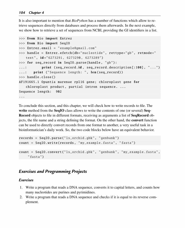
104 Chapter 4

It is also important to mention that BioPython has a number of functions which allow to re-trieve sequences directly from databases and process them afterwards. In the next example,we show how to retrieve a set of sequences from NCBI, providing the GI identifiers in a list.

>>> from Bio import Entrez>>> from Bio import SeqIO>>> Entrez.email = "example@gmail.com"

>>> handle = Entrez.efetch(db="nucleotide", rettype="gb", retmode="

text", id ="6273291, 6273290, 6273289")>>> f o r seq_record in SeqIO.parse(handle, "gb"):

...: p r i n t (seq_record. id , seq_record.description[:100], "...")

...: p r i n t ("Sequence length: ", l e n (seq_record))>>> handle.close()

AF191665.1 Opuntia marenae rpl16 gene; chloroplast gene f o rchloroplast product, partial intron sequence. ...

Sequence length: 902

...

To conclude this section, and this chapter, we will check how to write records to file. Thewrite method from the SeqIO class allows to write the contents of one (or several) Seq-Record objects to file in different formats, receiving as arguments a list of SeqRecord ob-jects, the file name and a string defining the format. On the other hand, the convert functioncan be used to directly convert records from one format to another, a very useful task in abioinformatician’s daily work. So, the two code blocks below have an equivalent behavior.

records = SeqIO.parse("ls_orchid.gbk", "genbank")

count = SeqIO.write(records, "my_example.fasta", "fasta")

count = SeqIO.convert("ls_orchid.gbk", "genbank", "my_example.fasta",

"fasta")

Exercises and Programming Projects

Exercises

1. Write a program that reads a DNA sequence, converts it to capital letters, and counts howmany nucleotides are purines and pyrimidines.

2. Write a program that reads a DNA sequence and checks if it is equal to its reverse com-plement.

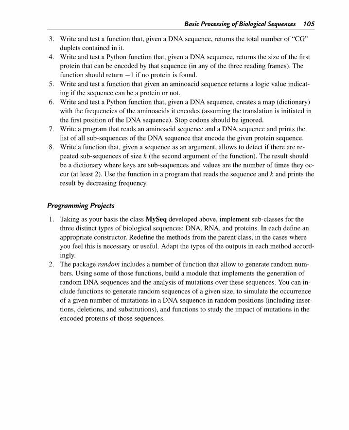
Basic Processing of Biological Sequences 105

3. Write and test a function that, given a DNA sequence, returns the total number of “CG”duplets contained in it.

4. Write and test a Python function that, given a DNA sequence, returns the size of the firstprotein that can be encoded by that sequence (in any of the three reading frames). Thefunction should return −1 if no protein is found.

5. Write and test a function that given an aminoacid sequence returns a logic value indicat-ing if the sequence can be a protein or not.

6. Write and test a Python function that, given a DNA sequence, creates a map (dictionary)with the frequencies of the aminoacids it encodes (assuming the translation is initiated inthe first position of the DNA sequence). Stop codons should be ignored.

7. Write a program that reads an aminoacid sequence and a DNA sequence and prints thelist of all sub-sequences of the DNA sequence that encode the given protein sequence.

8. Write a function that, given a sequence as an argument, allows to detect if there are re-peated sub-sequences of size k (the second argument of the function). The result shouldbe a dictionary where keys are sub-sequences and values are the number of times they oc-cur (at least 2). Use the function in a program that reads the sequence and k and prints theresult by decreasing frequency.

Programming Projects

1. Taking as your basis the class MySeq developed above, implement sub-classes for thethree distinct types of biological sequences: DNA, RNA, and proteins. In each define anappropriate constructor. Redefine the methods from the parent class, in the cases whereyou feel this is necessary or useful. Adapt the types of the outputs in each method accord-ingly.

2. The package random includes a number of function that allow to generate random num-bers. Using some of those functions, build a module that implements the generation ofrandom DNA sequences and the analysis of mutations over these sequences. You can in-clude functions to generate random sequences of a given size, to simulate the occurrenceof a given number of mutations in a DNA sequence in random positions (including inser-tions, deletions, and substitutions), and functions to study the impact of mutations in theencoded proteins of those sequences.

CHAPTER 5

Finding Patterns in SequencesIn this chapter, we discuss how to find patterns in sequences and the importance of this taskin Bioinformatics. We put forward the basic algorithms for pattern finding and discuss theircomplexity. Heuristic algorithms are presented to lower the average computational complex-ity of this task, by suitable pre-processing of the patterns to search. Also, we present regularexpressions as a way to find more flexible patterns in sequences, showing how these can beimplemented in Python, and discussing their biological relevance with some examples.

5.1 Introduction: Importance of Pattern Finding in Bioinformatics

Finding specific patterns within biological sequences is one of the most common tasks bioin-formaticians need to deal with, in their daily lives. Since relevant biological information is,as we have seen in the previous chapters (most notably in Chapter 3), kept in sequences, theanalysis of local patterns in those sequences is quite relevant.

Indeed, these patterns are in many cases closely connected to specific functions of themolecules represented by those sequences. Some examples include specific patterns corre-sponding to protein domains with a given function (e.g. binding sites for ligands in enzymesor for DNA molecules in regulatory proteins), or nucleotide patterns corresponding to parts ofDNA sequences, which may be associated to binding sites for regulation of gene expression(e.g. promoters, enhancers, transcription factors).

Thus, the identification of specified patterns in different types of sequences (DNA, RNA,proteins) is deeply connected to the association of sequences and sequence locations to di-verse biological functions. Also, the existence of numerous repeats, of different sizes, in thegenomes of living beings, and most pronouncedly in complex organisms (as humans), bringsan added importance to pattern finding.

Given the nature of the patterns we typically need to find, there are diverse tasks in Bioinfor-matics related to pattern finding, which diverge in the type of pattern to find, as well as in thesize and number of patterns and target sequence(s). Therefore, in this book, we will devotea few chapters to cover problems related to biological patterns in sequences, and the relatedconcept of sequence motifs.

Here, we will start by discussing algorithms for finding fixed patterns in larger sequences, ad-dressing the complexity of these algorithms and trying to make them more efficient. These

Bioinformatics Algorithms. DOI: 10.1016/B978-0-12-812520-5.00005-5Copyright © 2018 Elsevier Inc. All rights reserved. 107

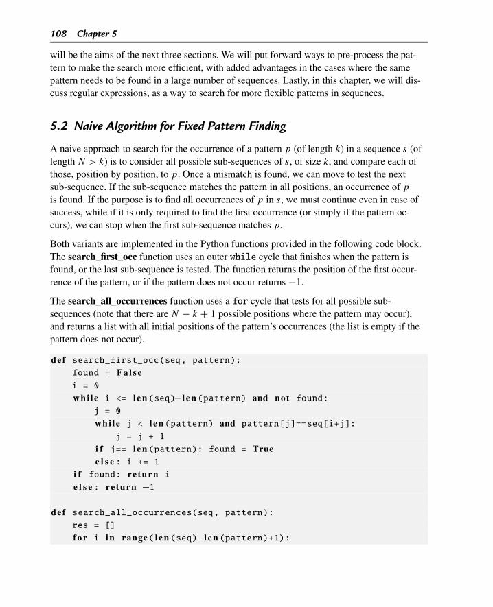
108 Chapter 5

will be the aims of the next three sections. We will put forward ways to pre-process the pat-tern to make the search more efficient, with added advantages in the cases where the samepattern needs to be found in a large number of sequences. Lastly, in this chapter, we will dis-cuss regular expressions, as a way to search for more flexible patterns in sequences.

5.2 Naive Algorithm for Fixed Pattern Finding

A naive approach to search for the occurrence of a pattern p (of length k) in a sequence s (oflength N > k) is to consider all possible sub-sequences of s, of size k, and compare each ofthose, position by position, to p. Once a mismatch is found, we can move to test the nextsub-sequence. If the sub-sequence matches the pattern in all positions, an occurrence of p

is found. If the purpose is to find all occurrences of p in s, we must continue even in case ofsuccess, while if it is only required to find the first occurrence (or simply if the pattern oc-curs), we can stop when the first sub-sequence matches p.

Both variants are implemented in the Python functions provided in the following code block.The search_first_occ function uses an outer while cycle that finishes when the pattern isfound, or the last sub-sequence is tested. The function returns the position of the first occur-rence of the pattern, or if the pattern does not occur returns −1.

The search_all_occurrences function uses a for cycle that tests for all possible sub-sequences (note that there are N − k + 1 possible positions where the pattern may occur),and returns a list with all initial positions of the pattern’s occurrences (the list is empty if thepattern does not occur).

def search_first_occ(seq, pattern):found = F a l s ei = 0

whi le i <= l e n (seq)−l e n (pattern) and not found:j = 0

whi le j < l e n (pattern) and pattern[j]==seq[i+j]:j = j + 1

i f j== l e n (pattern): found = Truee l s e : i += 1

i f found: re turn ie l s e : re turn −1

def search_all_occurrences(seq, pattern):res = []

f o r i in range( l e n (seq)−l e n (pattern)+1):

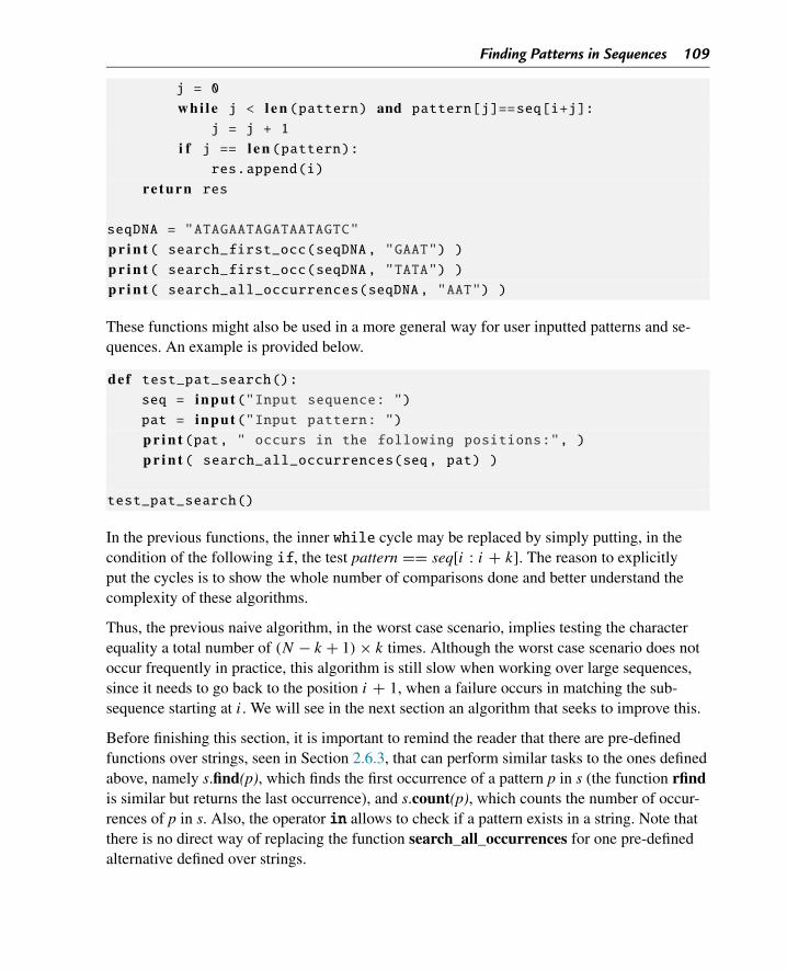
Finding Patterns in Sequences 109

j = 0

whi le j < l e n (pattern) and pattern[j]==seq[i+j]:j = j + 1

i f j == l e n (pattern):res.append(i)

re turn res

seqDNA = "ATAGAATAGATAATAGTC"

p r i n t ( search_first_occ(seqDNA, "GAAT") )p r i n t ( search_first_occ(seqDNA, "TATA") )p r i n t ( search_all_occurrences(seqDNA, "AAT") )

These functions might also be used in a more general way for user inputted patterns and se-quences. An example is provided below.

def test_pat_search():seq = input("Input sequence: ")pat = input("Input pattern: ")p r i n t (pat, " occurs in the following positions:", )p r i n t ( search_all_occurrences(seq, pat) )

test_pat_search()

In the previous functions, the inner while cycle may be replaced by simply putting, in thecondition of the following if, the test pattern == seq[i : i + k]. The reason to explicitlyput the cycles is to show the whole number of comparisons done and better understand thecomplexity of these algorithms.

Thus, the previous naive algorithm, in the worst case scenario, implies testing the characterequality a total number of (N − k + 1) × k times. Although the worst case scenario does notoccur frequently in practice, this algorithm is still slow when working over large sequences,since it needs to go back to the position i + 1, when a failure occurs in matching the sub-sequence starting at i. We will see in the next section an algorithm that seeks to improve this.

Before finishing this section, it is important to remind the reader that there are pre-definedfunctions over strings, seen in Section 2.6.3, that can perform similar tasks to the ones definedabove, namely s.find(p), which finds the first occurrence of a pattern p in s (the function rfindis similar but returns the last occurrence), and s.count(p), which counts the number of occur-rences of p in s. Also, the operator in allows to check if a pattern exists in a string. Note thatthere is no direct way of replacing the function search_all_occurrences for one pre-definedalternative defined over strings.

110 Chapter 5

5.3 Heuristic Algorithm: Boyer-Moore

As we saw in the previous section, the complexity of the naive algorithm can be penalizingin its computational efficiency. There are alternative algorithms which seek to improve theaverage computational efficiency of pattern searching, trying to use the structure of the patternto speed up the search saving a significant part of the pairwise symbol comparisons.

Although there are a number of alternatives for these algorithms, we will cover here only theBoyer-Moore algorithm, that although having in the worst case scenario a complexity similarto the naive algorithm, in most cases allows significant gains in performance. The algorithm isbased on two rules that allow to move forward more than one position in the target sequencein some situations.

As in the naive algorithm, the target sequence is scanned from the beginning to the end (left toright), but in this case the comparison of the pattern, with the sub-sequence in the text, is donefrom right to left. When there is a mismatch between the target sequence and the pattern, tworules can be applied to check if the process can be more efficient, by moving forward morethan one position in the sequence.

The first rule that can be applied is the bad-character rule, which states that we can advancethe pattern to the next occurrence (in the pattern) of the symbol in the sequence at the positionof the mismatch. If no occurrences of that symbol exist in the pattern, we can move forwardthe maximum number of symbols (until the end of the pattern).

Fig. 5.1A shows examples of three cases of a possible application of this rule. In the firstexample, the symbol in the sequence where the mismatch occurs (T) does not occur in thepattern, and therefore we can move forward the number of positions corresponding to placingthe pattern’s first symbol in the position following the mismatch. In the second example, thesymbol occurs in the pattern, and, thus, we can move the pattern so that the rightmost occur-rence of the symbol in the pattern matches the mismatched symbol in the sequence. The samehappens in the third example, but in this case we only move forward one position.

The other rule that may be applied is the good suffix rule, which states that, in case of amismatch, we can move forward to the next instance in the pattern of the part (suffix) thatmatched before (in the right) the mismatch.

Fig. 5.1B shows examples of the application of this rule. In the first case, the suffix “AC”matched and, therefore, the pattern moves to the next occurrence of this string in the pattern.The next case shows what happens when the suffix does not occur in the remaining of the pat-tern, allowing to move forward the pattern a number of positions equal to its length. The thirdexample shows a special case, where the full matching suffix (“CAC”) does not occur in thepattern, but a suffix does (“AC”).

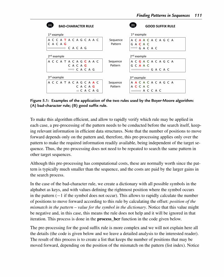
Finding Patterns in Sequences 111

Figure 5.1: Examples of the application of the two rules used by the Boyer-Moore algorithm:(A) bad-character rule; (B) good suffix rule.

To make this algorithm efficient, and allow to rapidly verify which rule may be applied ineach case, a pre-processing of the pattern needs to be conducted before the search itself, keep-ing relevant information in efficient data structures. Note that the number of positions to moveforward depends only on the pattern and, therefore, this pre-processing applies only over thepattern to make the required information readily available, being independent of the target se-quence. Thus, the pre-processing does not need to be repeated to search the same pattern inother target sequences.

Although this pre-processing has computational costs, these are normally worth since the pat-tern is typically much smaller than the sequence, and the costs are paid by the larger gains inthe search process.

In the case of the bad-character rule, we create a dictionary with all possible symbols in thealphabet as keys, and with values defining the rightmost position where the symbol occursin the pattern (−1 if the symbol does not occur). This allows to rapidly calculate the numberof positions to move forward according to this rule by calculating the offset: position of themismatch in the pattern – value for the symbol in the dictionary. Notice that this value mightbe negative and, in this case, this means the rule does not help and it will be ignored in thatiteration. This process is done in the process_bcr function in the code given below.

The pre-processing for the good suffix rule is more complex and we will not explain here allthe details (the code is given below and we leave a detailed analysis to the interested reader).The result of this process is to create a list that keeps the number of positions that may bemoved forward, depending on the position of the mismatch on the pattern (list index). Notice

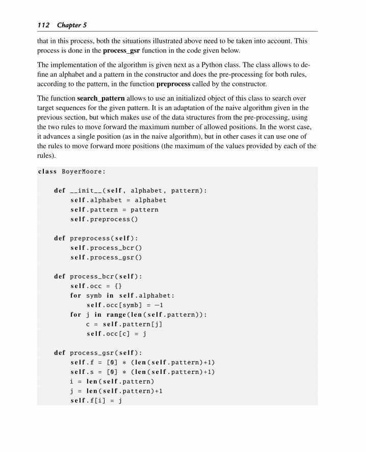
112 Chapter 5

that in this process, both the situations illustrated above need to be taken into account. Thisprocess is done in the process_gsr function in the code given below.

The implementation of the algorithm is given next as a Python class. The class allows to de-fine an alphabet and a pattern in the constructor and does the pre-processing for both rules,according to the pattern, in the function preprocess called by the constructor.

The function search_pattern allows to use an initialized object of this class to search overtarget sequences for the given pattern. It is an adaptation of the naive algorithm given in theprevious section, but which makes use of the data structures from the pre-processing, usingthe two rules to move forward the maximum number of allowed positions. In the worst case,it advances a single position (as in the naive algorithm), but in other cases it can use one ofthe rules to move forward more positions (the maximum of the values provided by each of therules).

c l a s s BoyerMoore:

def __init__( s e l f , alphabet, pattern):s e l f .alphabet = alphabets e l f .pattern = patterns e l f .preprocess()

def preprocess( s e l f ):s e l f .process_bcr()s e l f .process_gsr()

def process_bcr( s e l f ):s e l f .occ = {}f o r symb in s e l f .alphabet:

s e l f .occ[symb] = −1f o r j in range( l e n ( s e l f .pattern)):

c = s e l f .pattern[j]s e l f .occ[c] = j

def process_gsr( s e l f ):s e l f .f = [0] ∗ ( l e n ( s e l f .pattern)+1)s e l f .s = [0] ∗ ( l e n ( s e l f .pattern)+1)i = l e n ( s e l f .pattern)j = l e n ( s e l f .pattern)+1s e l f .f[i] = j

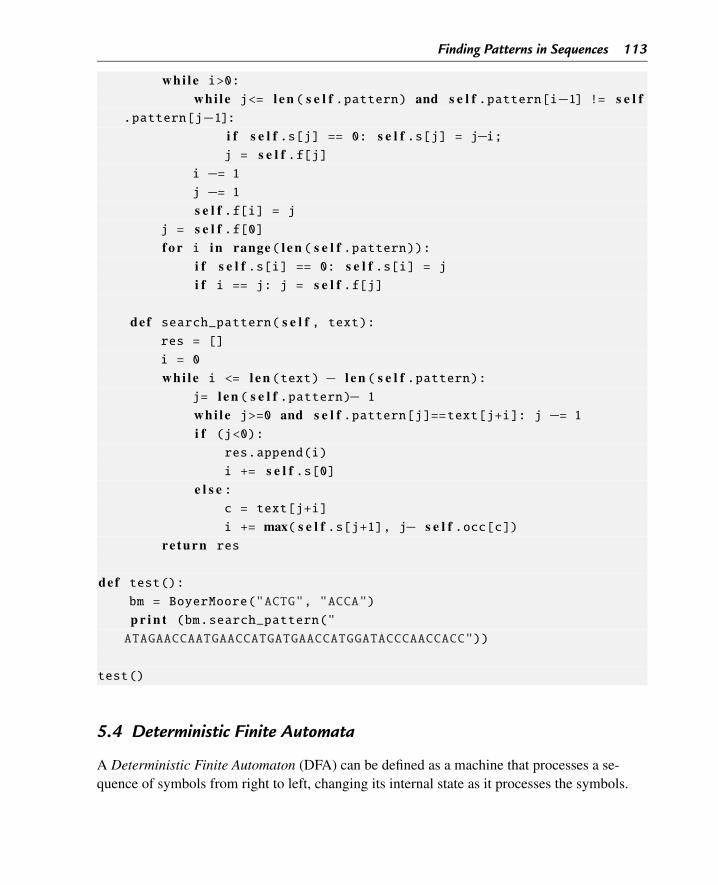
Finding Patterns in Sequences 113

whi le i>0:whi le j<= l e n ( s e l f .pattern) and s e l f .pattern[i−1] != s e l f

.pattern[j−1]:i f s e l f .s[j] == 0: s e l f .s[j] = j−i;j = s e l f .f[j]

i −= 1j −= 1s e l f .f[i] = j

j = s e l f .f[0]f o r i in range( l e n ( s e l f .pattern)):

i f s e l f .s[i] == 0: s e l f .s[i] = ji f i == j: j = s e l f .f[j]

def search_pattern( s e l f , text):res = []

i = 0

whi le i <= l e n (text) − l e n ( s e l f .pattern):j= l e n ( s e l f .pattern)− 1

whi le j>=0 and s e l f .pattern[j]==text[j+i]: j −= 1i f (j<0):

res.append(i)

i += s e l f .s[0]e l s e :

c = text[j+i]

i += max( s e l f .s[j+1], j− s e l f .occ[c])re turn res

def test():bm = BoyerMoore("ACTG", "ACCA")

p r i n t (bm.search_pattern("ATAGAACCAATGAACCATGATGAACCATGGATACCCAACCACC"))

test()

5.4 Deterministic Finite Automata

A Deterministic Finite Automaton (DFA) can be defined as a machine that processes a se-quence of symbols from right to left, changing its internal state as it processes the symbols.

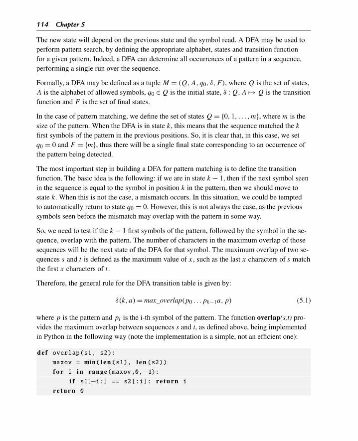
114 Chapter 5

The new state will depend on the previous state and the symbol read. A DFA may be used toperform pattern search, by defining the appropriate alphabet, states and transition functionfor a given pattern. Indeed, a DFA can determine all occurrences of a pattern in a sequence,performing a single run over the sequence.

Formally, a DFA may be defined as a tuple M = (Q,A,q0, δ,F ), where Q is the set of states,A is the alphabet of allowed symbols, q0 ∈ Q is the initial state, δ : Q,A �→ Q is the transitionfunction and F is the set of final states.

In the case of pattern matching, we define the set of states Q = {0,1, . . . ,m}, where m is thesize of the pattern. When the DFA is in state k, this means that the sequence matched the k

first symbols of the pattern in the previous positions. So, it is clear that, in this case, we setq0 = 0 and F = {m}, thus there will be a single final state corresponding to an occurrence ofthe pattern being detected.

The most important step in building a DFA for pattern matching is to define the transitionfunction. The basic idea is the following: if we are in state k − 1, then if the next symbol seenin the sequence is equal to the symbol in position k in the pattern, then we should move tostate k. When this is not the case, a mismatch occurs. In this situation, we could be temptedto automatically return to state q0 = 0. However, this is not always the case, as the previoussymbols seen before the mismatch may overlap with the pattern in some way.

So, we need to test if the k − 1 first symbols of the pattern, followed by the symbol in the se-quence, overlap with the pattern. The number of characters in the maximum overlap of thosesequences will be the next state of the DFA for that symbol. The maximum overlap of two se-quences s and t is defined as the maximum value of x, such as the last x characters of s matchthe first x characters of t .

Therefore, the general rule for the DFA transition table is given by:

δ(k, a) = max_overlap(p0 . . . pk−1a,p) (5.1)

where p is the pattern and pi is the i-th symbol of the pattern. The function overlap(s,t) pro-vides the maximum overlap between sequences s and t, as defined above, being implementedin Python in the following way (note the implementation is a simple, not an efficient one):

def overlap(s1, s2):

maxov = min( l e n (s1), l e n (s2))f o r i in range(maxov,0,−1):

i f s1[−i:] == s2[:i]: re turn ire turn 0

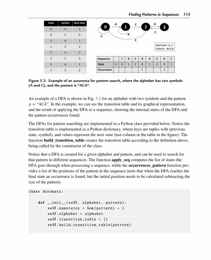
Finding Patterns in Sequences 115

Figure 5.2: Example of an automata for pattern search, where the alphabet has two symbols(A and C), and the pattern is “ACA”.

An example of a DFA is shown in Fig. 5.2 for an alphabet with two symbols and the patternp = “ACA”. In the example, we can see the transition table and its graphical representation,and the result of applying the DFA to a sequence, showing the internal states of the DFA andthe pattern occurrences found.

The DFAs for pattern searching are implemented in a Python class provided below. Notice thetransition table is implemented as a Python dictionary, where keys are tuples with (previousstate, symbol), and values represent the next state (last column in the table in the figure). Thefunction build_transition_table creates the transition table according to the definition above,being called by the constructor of the class.

Notice that a DFA is created for a given alphabet and pattern, and can be used to search forthat pattern in different sequences. The function apply_seq computes the list of states theDFA goes through when processing a sequence, while the occurrences_pattern function pro-vides a list of the positions of the pattern in the sequence (note that when the DFA reaches thefinal state an occurrence is found, but the initial position needs to be calculated subtracting thesize of the pattern).

c l a s s Automata:

def __init__( s e l f , alphabet, pattern):s e l f .numstates = l e n (pattern) + 1s e l f .alphabet = alphabets e l f .transition_table = {}s e l f .build_transition_table(pattern)

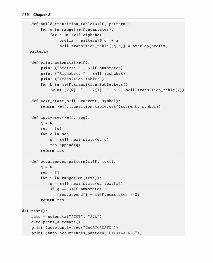
116 Chapter 5

def build_transition_table( s e l f , pattern):f o r q in range( s e l f .numstates):

f o r a in s e l f .alphabet:prefix = pattern[0:q] + a

s e l f .transition_table[(q,a)] = overlap(prefix,pattern)

def print_automata( s e l f ):p r i n t ("States: " , s e l f .numstates)p r i n t ("Alphabet: " , s e l f .alphabet)p r i n t ("Transition table:")f o r k in s e l f .transition_table.keys():

p r i n t (k[0], ",", k[1], " −> ", s e l f .transition_table[k])

def next_state( s e l f , current, symbol):re turn s e l f .transition_table.get((current, symbol))

def apply_seq( s e l f , seq):q = 0

res = [q]

f o r c in seq:

q = s e l f .next_state(q, c)res.append(q)

re turn res

def occurrences_pattern( s e l f , text):q = 0

res = []

f o r i in range( l e n (text)):q = s e l f .next_state(q, text[i])i f q == s e l f .numstates−1:

res.append(i − s e l f .numstates + 2)re turn res

def test():auto = Automata("ACGT", "ACA")

auto.print_automata()

p r i n t (auto.apply_seq("CACATGACATG"))p r i n t (auto.occurrences_pattern("CACATGACATG"))

Finding Patterns in Sequences 117

test()

5.5 Finding Flexible Patterns: Regular Expressions

5.5.1 Definitions and Regular Expressions in Python

Regular expressions (REs) are a programming concept, that exists in all modern program-ming languages, that allow to define patterns to search in strings in a flexible manner. REsare defined as strings, where some of the characters are not used as regular characters, butrather as meta-characters to represent patterns. While regular characters in an RE only matchthemselves in a search process, meta-characters may offer many alternatives for matching de-pending on their meaning.

One of the most used meta-characters is the dot (.), that matches any character in a string.Thus, the RE “...” will match any string of length 3. Some of the meta-characters are used tomodify the predecessor character (or set of characters) by allowing repetitions of patterns, asfollows:

• * – zero or more repetitions of the pattern to which it applies;• + – one or more repetitions of the pattern;• ? – zero or one repetitions (pattern may occur or not);• {n} – exactly n repetitions, where n is an integer;• {m,n} – between m and n repetitions, where m and n are integers and n >= m.

The previous “modifiers” may be applied to a single character or to a group of characters, thatcan be defined using regular brackets. On the other hand, square brackets are used to definepossible lists of characters that match. This syntax is quite useful as the following examplesshow:

• [A-Z] – matches any upper-case letter;• [a-z] – matches any lower-case letter;• [A-Za-z] – matches any letter;• [0-9] – matches any digit;• [ACTGactg] – matches a DNA nucleotide symbol (upper or lower case);• [ACDEFGHIKLMNPQRSTVWY] – matches an aminoacid symbol (upper case).

If the ˆ symbol is put before the list, it is negated, i.e. it will match all characters not includedin the list. Thus, “[ˆ0-9]” matches with non-digits.

Combining these definitions with the previous ones, it is easy to define an RE for a nat-ural number as the string “[0-9]*”, or to define a DNA sequence as “[ACTGactg]*”,

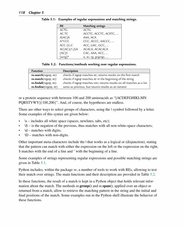
118 Chapter 5

Table 5.1: Examples of regular expressions and matching strings.

RE Matching stringsACTG ACTGAC.TC ACCTC, ACCTC, ACXTC, ...A[AC]A AAA, ACAA*CCC CCC, ACCC, AACCC, ...ACC |G.C ACC, GAC, GCC, ...AC(AC){1,2}A ACACA, ACACACA[AC]3 CAC, AAA, ACC, ...[actg]* a, ac, tg, gcgctgc, ...

Table 5.2: Functions/methods working over regular expressions.

Function Descriptionre.search(regexp, str) checks if regexp matches str; returns results on the first matchre.match(regexp, str) checks if regexp matches str in the beginning of the stringre.findall(regexp, str) checks if regexp matches vstr; returns results on all matches as a listre.finditer(regexp, str) same as previous, but returns results as an iterator

or a protein sequence with between 100 and 200 aminoacids as “[ACDEFGHIKLMNPQRSTVWY]{100,200}”. And, of course, the hypotheses are endless.

There are other ways to select groups of characters, using the \ symbol followed by a letter.Some examples of this syntax are given below:

• \s – includes all white space (spaces, newlines, tabs, etc);• \S – is the negation of the previous, thus matches with all non-white-space characters;• \d – matches with digits;• \D – matches with non-digits.

Other important meta-characters include the | that works as a logical or (disjunction), statingthat the pattern can match with either the expression on the left or the expression on the right,$ matches with the end of a line and ˆ with the beginning of a line.

Some examples of strings representing regular expressions and possible matching strings aregiven in Table 5.1.

Python includes, within the package re, a number of tools to work with REs, allowing to testtheir match over strings. The main functions and their description are provided in Table 5.2.

In these functions, the result of a match is kept in a Python object that holds relevant infor-mation about the match. The methods m.group() and m.span(), applied over an object mreturned from a match, allow to retrieve the matching pattern in the string and the initial andfinal positions of the match. Some examples run in the Python shell illustrate the behavior ofthese functions.

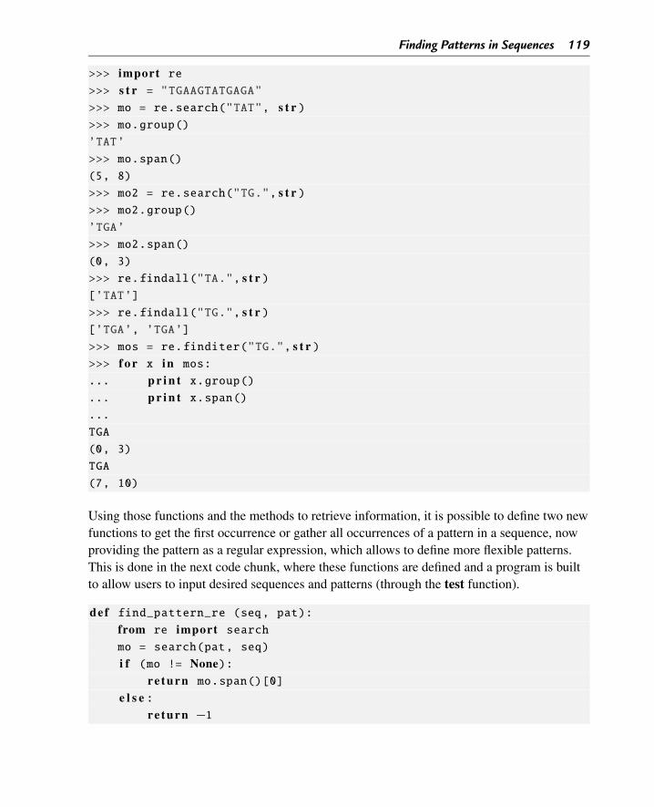
Finding Patterns in Sequences 119

>>> import re>>> s t r = "TGAAGTATGAGA">>> mo = re.search("TAT", s t r )>>> mo.group()

’TAT’

>>> mo.span()

(5, 8)

>>> mo2 = re.search("TG.", s t r )>>> mo2.group()

’TGA’

>>> mo2.span()

(0, 3)

>>> re.findall("TA.", s t r )[’TAT’]

>>> re.findall("TG.", s t r )[’TGA’, ’TGA’]

>>> mos = re.finditer("TG.", s t r )>>> f o r x in mos:

... p r i n t x.group()

... p r i n t x.span()

...

TGA

(0, 3)

TGA

(7, 10)

Using those functions and the methods to retrieve information, it is possible to define two newfunctions to get the first occurrence or gather all occurrences of a pattern in a sequence, nowproviding the pattern as a regular expression, which allows to define more flexible patterns.This is done in the next code chunk, where these functions are defined and a program is builtto allow users to input desired sequences and patterns (through the test function).

def find_pattern_re (seq, pat):from re import searchmo = search(pat, seq)

i f (mo != None):re turn mo.span()[0]

e l s e :re turn −1

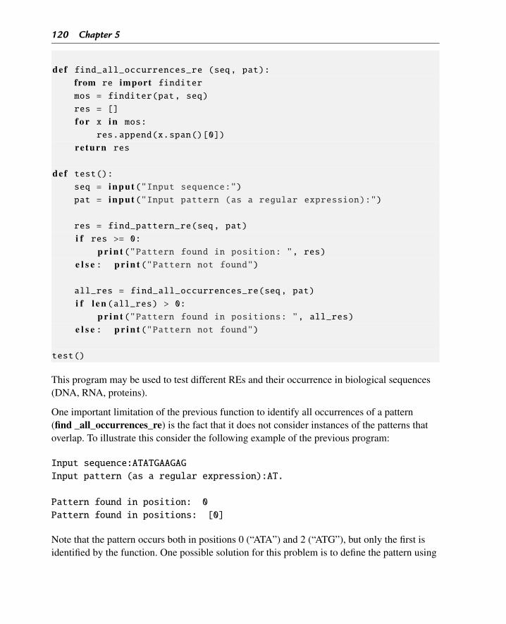
120 Chapter 5

def find_all_occurrences_re (seq, pat):from re import finditermos = finditer(pat, seq)

res = []

f o r x in mos:

res.append(x.span()[0])

re turn res

def test():seq = input("Input sequence:")pat = input("Input pattern (as a regular expression):")

res = find_pattern_re(seq, pat)

i f res >= 0:p r i n t ("Pattern found in position: ", res)

e l s e : p r i n t ("Pattern not found")

all_res = find_all_occurrences_re(seq, pat)

i f l e n (all_res) > 0:p r i n t ("Pattern found in positions: ", all_res)

e l s e : p r i n t ("Pattern not found")

test()

This program may be used to test different REs and their occurrence in biological sequences(DNA, RNA, proteins).

One important limitation of the previous function to identify all occurrences of a pattern(find _all_occurrences_re) is the fact that it does not consider instances of the patterns thatoverlap. To illustrate this consider the following example of the previous program:

Input sequence:ATATGAAGAG

Input pattern (as a regular expression):AT.

Pattern found in position: 0

Pattern found in positions: [0]

Note that the pattern occurs both in positions 0 (“ATA”) and 2 (“ATG”), but only the first isidentified by the function. One possible solution for this problem is to define the pattern using

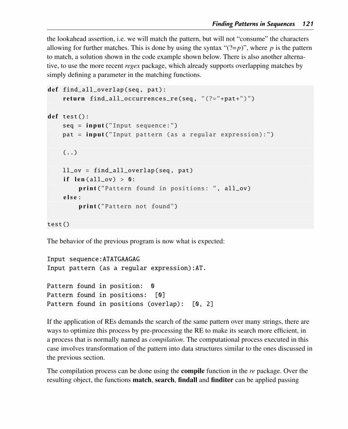
Finding Patterns in Sequences 121

the lookahead assertion, i.e. we will match the pattern, but will not “consume” the charactersallowing for further matches. This is done by using the syntax “(?=p)”, where p is the patternto match, a solution shown in the code example shown below. There is also another alterna-tive, to use the more recent regex package, which already supports overlapping matches bysimply defining a parameter in the matching functions.

def find_all_overlap(seq, pat):re turn find_all_occurrences_re(seq, "(?="+pat+")")

def test():seq = input("Input sequence:")pat = input("Input pattern (as a regular expression):")

(..)

ll_ov = find_all_overlap(seq, pat)

i f l e n (all_ov) > 0:p r i n t ("Pattern found in positions: ", all_ov)

e l s e :p r i n t ("Pattern not found")

test()

The behavior of the previous program is now what is expected:

Input sequence:ATATGAAGAG

Input pattern (as a regular expression):AT.

Pattern found in position: 0

Pattern found in positions: [0]

Pattern found in positions (overlap): [0, 2]

If the application of REs demands the search of the same pattern over many strings, there areways to optimize this process by pre-processing the RE to make its search more efficient, ina process that is normally named as compilation. The computational process executed in thiscase involves transformation of the pattern into data structures similar to the ones discussed inthe previous section.

The compilation process can be done using the compile function in the re package. Over theresulting object, the functions match, search, findall and finditer can be applied passing

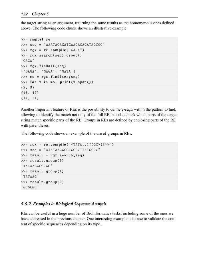
122 Chapter 5

the target string as an argument, returning the same results as the homonymous ones definedabove. The following code chunk shows an illustrative example.

>>> import re>>> seq = "AAATAGAGATGAAGAGAGATAGCGC"

>>> rgx = re. compi le("GA.A")>>> rgx.search(seq).group()

’GAGA’

>>> rgx.findall(seq)

[’GAGA’, ’GAGA’, ’GATA’]

>>> mo = rgx.finditer(seq)

>>> f o r x in mo: p r i n t (x.span())(5, 9)

(13, 17)

(17, 21)

Another important feature of REs is the possibility to define groups within the pattern to find,allowing to identify the match not only of the full RE, but also check which parts of the targetstring match specific parts of the RE. Groups in REs are defined by enclosing parts of the REwith parentheses.

The following code shows an example of the use of groups in REs.

>>> rgx = re. compi le("(TATA..)((GC){3})")>>> seq = "ATATAAGGCGCGCGCTTATGCGC"

>>> result = rgx.search(seq)

>>> result.group(0)

’TATAAGGCGCGC’

>>> result.group(1)

’TATAAG’

>>> result.group(2)

’GCGCGC’

5.5.2 Examples in Biological Sequence Analysis

REs can be useful in a huge number of Bioinformatics tasks, including some of the ones wehave addressed in the previous chapter. One interesting example is its use to validate the con-tent of specific sequences depending on its type.

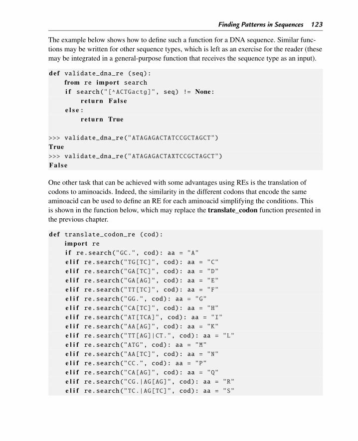
Finding Patterns in Sequences 123

The example below shows how to define such a function for a DNA sequence. Similar func-tions may be written for other sequence types, which is left as an exercise for the reader (thesemay be integrated in a general-purpose function that receives the sequence type as an input).

def validate_dna_re (seq):from re import searchi f search("[^ACTGactg]", seq) != None:

re turn F a l s ee l s e :

re turn True

>>> validate_dna_re("ATAGAGACTATCCGCTAGCT")

True>>> validate_dna_re("ATAGAGACTAXTCCGCTAGCT")

F a l s e

One other task that can be achieved with some advantages using REs is the translation ofcodons to aminoacids. Indeed, the similarity in the different codons that encode the sameaminoacid can be used to define an RE for each aminoacid simplifying the conditions. Thisis shown in the function below, which may replace the translate_codon function presented inthe previous chapter.

def translate_codon_re (cod):import rei f re.search("GC.", cod): aa = "A"e l i f re.search("TG[TC]", cod): aa = "C"e l i f re.search("GA[TC]", cod): aa = "D"e l i f re.search("GA[AG]", cod): aa = "E"e l i f re.search("TT[TC]", cod): aa = "F"e l i f re.search("GG.", cod): aa = "G"e l i f re.search("CA[TC]", cod): aa = "H"e l i f re.search("AT[TCA]", cod): aa = "I"e l i f re.search("AA[AG]", cod): aa = "K"e l i f re.search("TT[AG]|CT.", cod): aa = "L"e l i f re.search("ATG", cod): aa = "M"e l i f re.search("AA[TC]", cod): aa = "N"e l i f re.search("CC.", cod): aa = "P"e l i f re.search("CA[AG]", cod): aa = "Q"e l i f re.search("CG.|AG[AG]", cod): aa = "R"e l i f re.search("TC.|AG[TC]", cod): aa = "S"

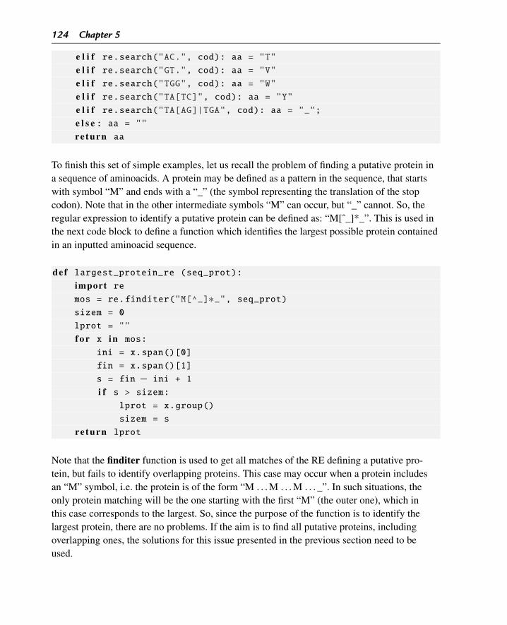
124 Chapter 5

e l i f re.search("AC.", cod): aa = "T"e l i f re.search("GT.", cod): aa = "V"e l i f re.search("TGG", cod): aa = "W"e l i f re.search("TA[TC]", cod): aa = "Y"e l i f re.search("TA[AG]|TGA", cod): aa = "_";e l s e : aa = ""re turn aa

To finish this set of simple examples, let us recall the problem of finding a putative protein ina sequence of aminoacids. A protein may be defined as a pattern in the sequence, that startswith symbol “M” and ends with a “_” (the symbol representing the translation of the stopcodon). Note that in the other intermediate symbols “M” can occur, but “_” cannot. So, theregular expression to identify a putative protein can be defined as: “M[ˆ_]*_”. This is used inthe next code block to define a function which identifies the largest possible protein containedin an inputted aminoacid sequence.

def largest_protein_re (seq_prot):import remos = re.finditer("M[^_]∗_", seq_prot)sizem = 0

lprot = ""

f o r x in mos:

ini = x.span()[0]

fin = x.span()[1]

s = fin − ini + 1

i f s > sizem:lprot = x.group()

sizem = s

re turn lprot

Note that the finditer function is used to get all matches of the RE defining a putative pro-tein, but fails to identify overlapping proteins. This case may occur when a protein includesan “M” symbol, i.e. the protein is of the form “M . . . M . . . M . . . _”. In such situations, theonly protein matching will be the one starting with the first “M” (the outer one), which inthis case corresponds to the largest. So, since the purpose of the function is to identify thelargest protein, there are no problems. If the aim is to find all putative proteins, includingoverlapping ones, the solutions for this issue presented in the previous section need to beused.

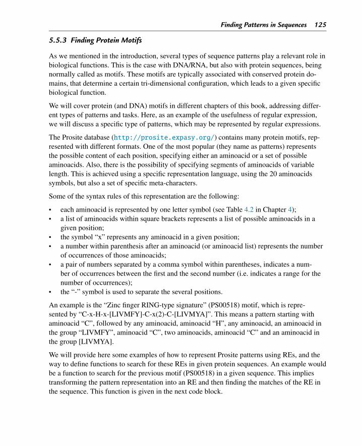
Finding Patterns in Sequences 125

5.5.3 Finding Protein Motifs

As we mentioned in the introduction, several types of sequence patterns play a relevant role inbiological functions. This is the case with DNA/RNA, but also with protein sequences, beingnormally called as motifs. These motifs are typically associated with conserved protein do-mains, that determine a certain tri-dimensional configuration, which leads to a given specificbiological function.

We will cover protein (and DNA) motifs in different chapters of this book, addressing differ-ent types of patterns and tasks. Here, as an example of the usefulness of regular expression,we will discuss a specific type of patterns, which may be represented by regular expressions.

The Prosite database (http://prosite.expasy.org/) contains many protein motifs, rep-resented with different formats. One of the most popular (they name as patterns) representsthe possible content of each position, specifying either an aminoacid or a set of possibleaminoacids. Also, there is the possibility of specifying segments of aminoacids of variablelength. This is achieved using a specific representation language, using the 20 aminoacidssymbols, but also a set of specific meta-characters.

Some of the syntax rules of this representation are the following:

• each aminoacid is represented by one letter symbol (see Table 4.2 in Chapter 4);• a list of aminoacids within square brackets represents a list of possible aminoacids in a

given position;• the symbol “x” represents any aminoacid in a given position;• a number within parenthesis after an aminoacid (or aminoacid list) represents the number

of occurrences of those aminoacids;• a pair of numbers separated by a comma symbol within parentheses, indicates a num-

ber of occurrences between the first and the second number (i.e. indicates a range for thenumber of occurrences);

• the “-” symbol is used to separate the several positions.

An example is the “Zinc finger RING-type signature” (PS00518) motif, which is repre-sented by “C-x-H-x-[LIVMFY]-C-x(2)-C-[LIVMYA]”. This means a pattern starting withaminoacid “C”, followed by any aminoacid, aminoacid “H”, any aminoacid, an aminoacid inthe group “LIVMFY”, aminoacid “C”, two aminoacids, aminoacid “C” and an aminoacid inthe group [LIVMYA].

We will provide here some examples of how to represent Prosite patterns using REs, and theway to define functions to search for these REs in given protein sequences. An example wouldbe a function to search for the previous motif (PS00518) in a given sequence. This impliestransforming the pattern representation into an RE and then finding the matches of the RE inthe sequence. This function is given in the next code block.

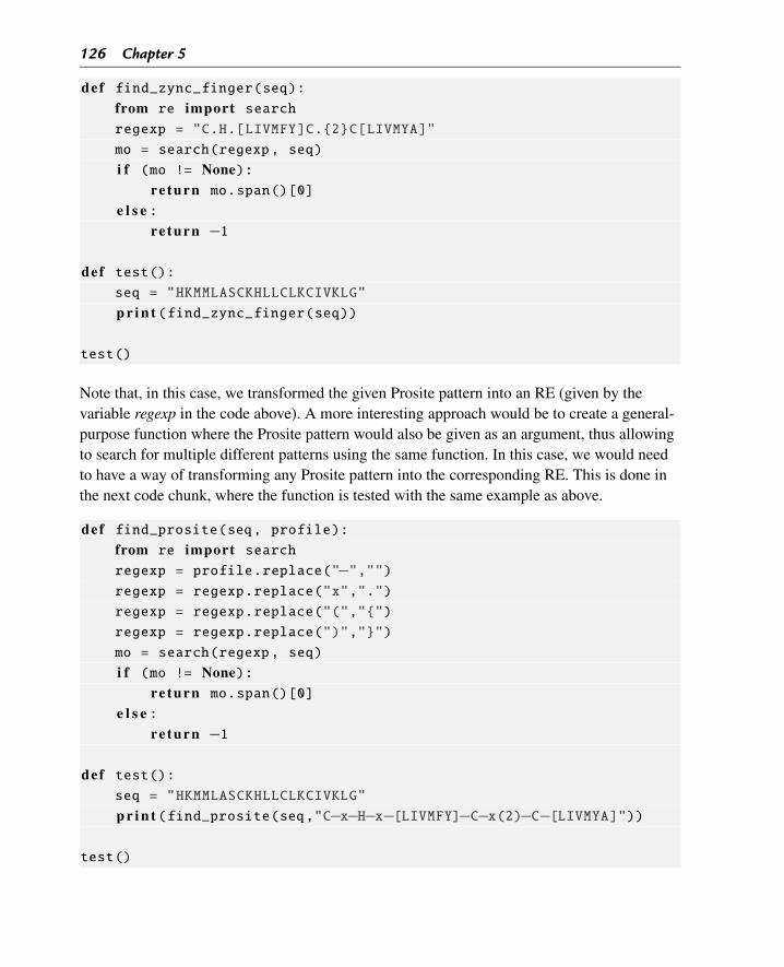
126 Chapter 5

def find_zync_finger(seq):from re import searchregexp = "C.H.[LIVMFY]C.{2}C[LIVMYA]"

mo = search(regexp, seq)

i f (mo != None):re turn mo.span()[0]

e l s e :re turn −1

def test():seq = "HKMMLASCKHLLCLKCIVKLG"

p r i n t (find_zync_finger(seq))

test()

Note that, in this case, we transformed the given Prosite pattern into an RE (given by thevariable regexp in the code above). A more interesting approach would be to create a general-purpose function where the Prosite pattern would also be given as an argument, thus allowingto search for multiple different patterns using the same function. In this case, we would needto have a way of transforming any Prosite pattern into the corresponding RE. This is done inthe next code chunk, where the function is tested with the same example as above.

def find_prosite(seq, profile):from re import searchregexp = profile.replace("−","")regexp = regexp.replace("x",".")

regexp = regexp.replace("(","{")

regexp = regexp.replace(")","}")

mo = search(regexp, seq)

i f (mo != None):re turn mo.span()[0]

e l s e :re turn −1

def test():seq = "HKMMLASCKHLLCLKCIVKLG"

p r i n t (find_prosite(seq,"C−x−H−x−[LIVMFY]−C−x(2)−C−[LIVMYA]"))

test()

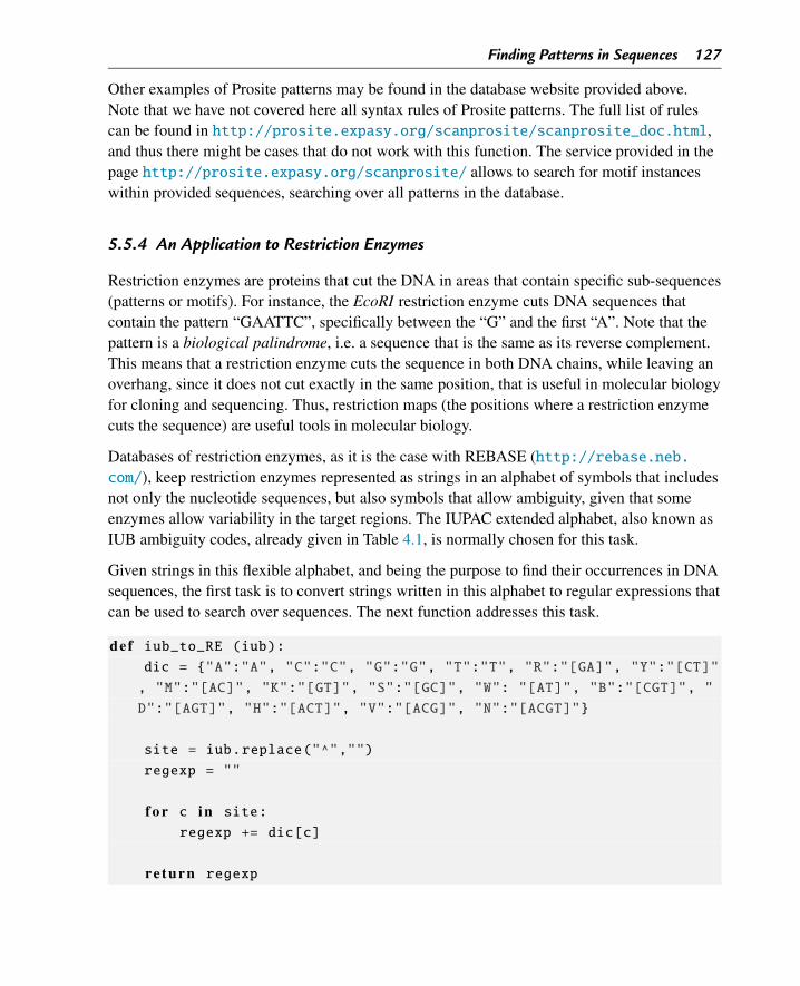
Finding Patterns in Sequences 127

Other examples of Prosite patterns may be found in the database website provided above.Note that we have not covered here all syntax rules of Prosite patterns. The full list of rulescan be found in http://prosite.expasy.org/scanprosite/scanprosite_doc.html,and thus there might be cases that do not work with this function. The service provided in thepage http://prosite.expasy.org/scanprosite/ allows to search for motif instanceswithin provided sequences, searching over all patterns in the database.

5.5.4 An Application to Restriction Enzymes

Restriction enzymes are proteins that cut the DNA in areas that contain specific sub-sequences(patterns or motifs). For instance, the EcoRI restriction enzyme cuts DNA sequences thatcontain the pattern “GAATTC”, specifically between the “G” and the first “A”. Note that thepattern is a biological palindrome, i.e. a sequence that is the same as its reverse complement.This means that a restriction enzyme cuts the sequence in both DNA chains, while leaving anoverhang, since it does not cut exactly in the same position, that is useful in molecular biologyfor cloning and sequencing. Thus, restriction maps (the positions where a restriction enzymecuts the sequence) are useful tools in molecular biology.

Databases of restriction enzymes, as it is the case with REBASE (http://rebase.neb.com/), keep restriction enzymes represented as strings in an alphabet of symbols that includesnot only the nucleotide sequences, but also symbols that allow ambiguity, given that someenzymes allow variability in the target regions. The IUPAC extended alphabet, also known asIUB ambiguity codes, already given in Table 4.1, is normally chosen for this task.

Given strings in this flexible alphabet, and being the purpose to find their occurrences in DNAsequences, the first task is to convert strings written in this alphabet to regular expressions thatcan be used to search over sequences. The next function addresses this task.

def iub_to_RE (iub):dic = {"A":"A", "C":"C", "G":"G", "T":"T", "R":"[GA]", "Y":"[CT]"

, "M":"[AC]", "K":"[GT]", "S":"[GC]", "W": "[AT]", "B":"[CGT]", "

D":"[AGT]", "H":"[ACT]", "V":"[ACG]", "N":"[ACGT]"}

site = iub.replace("^","")

regexp = ""

f o r c in site:

regexp += dic[c]

re turn regexp

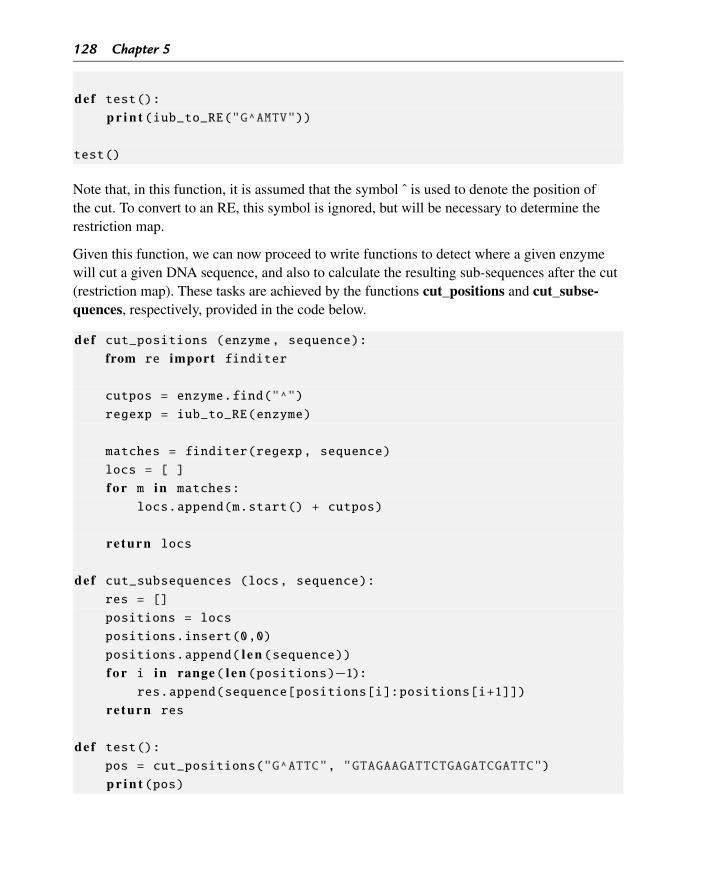
128 Chapter 5

def test():p r i n t (iub_to_RE("G^AMTV"))

test()

Note that, in this function, it is assumed that the symbol ˆ is used to denote the position ofthe cut. To convert to an RE, this symbol is ignored, but will be necessary to determine therestriction map.

Given this function, we can now proceed to write functions to detect where a given enzymewill cut a given DNA sequence, and also to calculate the resulting sub-sequences after the cut(restriction map). These tasks are achieved by the functions cut_positions and cut_subse-quences, respectively, provided in the code below.

def cut_positions (enzyme, sequence):from re import finditer

cutpos = enzyme.find("^")

regexp = iub_to_RE(enzyme)

matches = finditer(regexp, sequence)

locs = [ ]

f o r m in matches:

locs.append(m.start() + cutpos)

re turn locs

def cut_subsequences (locs, sequence):res = []

positions = locs

positions.insert(0,0)

positions.append( l e n (sequence))f o r i in range( l e n (positions)−1):

res.append(sequence[positions[i]:positions[i+1]])

re turn res

def test():pos = cut_positions("G^ATTC", "GTAGAAGATTCTGAGATCGATTC")

p r i n t (pos)

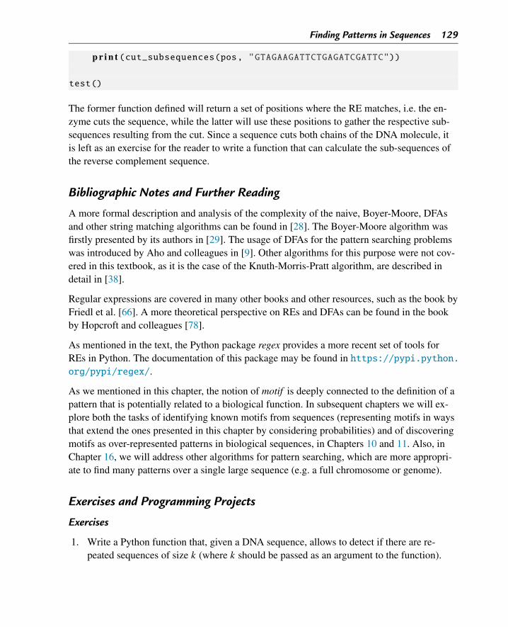
Finding Patterns in Sequences 129

p r i n t (cut_subsequences(pos, "GTAGAAGATTCTGAGATCGATTC"))

test()

The former function defined will return a set of positions where the RE matches, i.e. the en-zyme cuts the sequence, while the latter will use these positions to gather the respective sub-sequences resulting from the cut. Since a sequence cuts both chains of the DNA molecule, itis left as an exercise for the reader to write a function that can calculate the sub-sequences ofthe reverse complement sequence.

Bibliographic Notes and Further Reading

A more formal description and analysis of the complexity of the naive, Boyer-Moore, DFAsand other string matching algorithms can be found in [28]. The Boyer-Moore algorithm wasfirstly presented by its authors in [29]. The usage of DFAs for the pattern searching problemswas introduced by Aho and colleagues in [9]. Other algorithms for this purpose were not cov-ered in this textbook, as it is the case of the Knuth-Morris-Pratt algorithm, are described indetail in [38].

Regular expressions are covered in many other books and other resources, such as the book byFriedl et al. [66]. A more theoretical perspective on REs and DFAs can be found in the bookby Hopcroft and colleagues [78].

As mentioned in the text, the Python package regex provides a more recent set of tools forREs in Python. The documentation of this package may be found in https://pypi.python.org/pypi/regex/.

As we mentioned in this chapter, the notion of motif is deeply connected to the definition of apattern that is potentially related to a biological function. In subsequent chapters we will ex-plore both the tasks of identifying known motifs from sequences (representing motifs in waysthat extend the ones presented in this chapter by considering probabilities) and of discoveringmotifs as over-represented patterns in biological sequences, in Chapters 10 and 11. Also, inChapter 16, we will address other algorithms for pattern searching, which are more appropri-ate to find many patterns over a single large sequence (e.g. a full chromosome or genome).

Exercises and Programming Projects

Exercises

1. Write a Python function that, given a DNA sequence, allows to detect if there are re-peated sequences of size k (where k should be passed as an argument to the function).

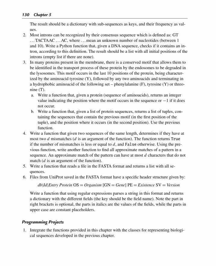
130 Chapter 5

The result should be a dictionary with sub-sequences as keys, and their frequency as val-ues.

2. Most introns can be recognized by their consensus sequence which is defined as: GT. . . TACTAAC . . . AC, where . . . mean an unknown number of nucleotides (between 1and 10). Write a Python function that, given a DNA sequence, checks if it contains an in-tron, according to this definition. The result should be a list with all initial positions of theintrons (empty list if there are none).

3. In many proteins present in the membrane, there is a conserved motif that allows them tobe identified in the transport process of these protein by the endosomes to be degraded inthe lysosomes. This motif occurs in the last 10 positions of the protein, being character-ized by the aminoacid tyrosine (Y), followed by any two aminoacids and terminating ina hydrophobic aminoacid of the following set – phenylalanine (F), tyrosine (Y) or threo-nine (T).a. Write a function that, given a protein (sequence of aminoacids), returns an integer

value indicating the position where the motif occurs in the sequence or −1 if it doesnot occur.

b. Write a function that, given a list of protein sequences, returns a list of tuples, con-taining the sequences that contain the previous motif (in the first position of thetuple), and the position where it occurs (in the second position). Use the previousfunction.

4. Write a function that given two sequences of the same length, determines if they have atmost two d mismatches (d is an argument of the function). The function returns Trueif the number of mismatches is less or equal to d , and False otherwise. Using the pre-vious function, write another function to find all approximate matches of a pattern in asequence. An approximate match of the pattern can have at most d characters that do notmatch (d is an argument of the function).

5. Write a function that reads a file in the FASTA format and returns a list with all se-quences.

6. Files from UniProt saved in the FASTA format have a specific header structure given by:

db|Id|Entry Protein OS = Organism [GN = Gene] PE = Existence SV = Version

Write a function that using regular expressions parses a string in this format and returnsa dictionary with the different fields (the key should be the field name). Note the part inright brackets is optional, the parts in italics are the values of the fields, while the parts inupper case are constant placeholders.

Programming Projects

1. Integrate the functions provided in this chapter with the classes for representing biologi-cal sequences developed in the previous chapter.

Finding Patterns in Sequences 131

2. Consider the Genbank file format, used by NCBI to keep sequences and their annotations.Write functions to read a Genbank record and parse it, using regular expressions. Fromthe record, you should extract the identifiers (ACCESSION number, GI, etc), the size ofthe sequence, its definition, the organism, the full sequence. Also, you should extract theinformation from the features, including for each feature, the source, the location, anda dictionary with the qualifiers. Check Section 4.8 to see how BioPython handles thesefiles.

CHAPTER 6

Pairwise Sequence Alignment

In this chapter, we show that to assess pairwise sequence similarity, we need to align the se-quences. We define the alignment process as an optimization problem and discuss efficientalgorithms based on dynamic programming for these problems, both considering global andlocal alignments. The implementation of these algorithms in Python is put forward and dis-cussed. We also address BioPython functions to align pairs of sequences.

6.1 Introduction: Comparing Sequences and Sequence Alignment

One of the major contributions that Bioinformatics can bring to biological research is thepossibility to help in elucidating the function of given genes or the proteins they encode.A common approach to address these tasks is to generate hypotheses regarding their bio-logical function, based on the similarity of their sequences to others that have a determinedfunction, preferably with an experimental validation.

Indeed, what we are trying to achieve here is to infer homology, i.e. the existence of sharedancestry, based on sequence similarity. It is important to emphasize that these concepts are notequivalent. However, in practice, sequences that show a high degree of similarity have a highprobability of being homologous and sharing similar functions. This probability grows withthe increase in the similarity degree. When the similarity reaches high levels (the definition ofa proper threshold is unfortunately not obvious), we can infer function with some credibility,although the ideal is always to verify experimentally.

So, in this scenario, to be able to compare pairs of sequences is of foremost importance. Ata first sight, this seems a straightforward problem. Indeed, we can intuitively define similarsequences as those who share the same symbols in the same order. Thus, this seems like atrivial computational task, but this is not the case.

We need to consider the sources of variability between sequences that share a common an-cestor: mutations. Biological mutations can lead to the changes in one or more nucleotides,but there are also insertions and deletions of nucleotides. These make the comparison of se-quences more complex, since we can not compare sequences position by position.

To overcome this difficulty, we need to resort to sequence alignment, the computational pro-cedure of seeking shared individual characters in both sequences, keeping the same order. The

Bioinformatics Algorithms. DOI: 10.1016/B978-0-12-812520-5.00006-7Copyright © 2018 Elsevier Inc. All rights reserved. 133

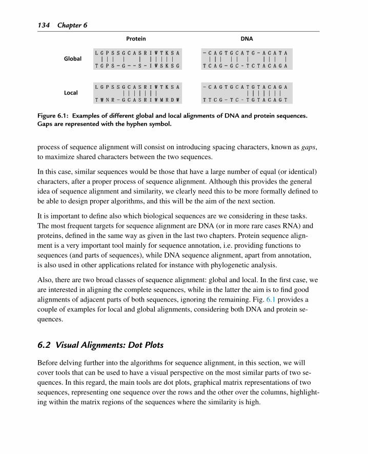
134 Chapter 6

Figure 6.1: Examples of different global and local alignments of DNA and protein sequences.Gaps are represented with the hyphen symbol.

process of sequence alignment will consist on introducing spacing characters, known as gaps,to maximize shared characters between the two sequences.

In this case, similar sequences would be those that have a large number of equal (or identical)characters, after a proper process of sequence alignment. Although this provides the generalidea of sequence alignment and similarity, we clearly need this to be more formally defined tobe able to design proper algorithms, and this will be the aim of the next section.

It is important to define also which biological sequences are we considering in these tasks.The most frequent targets for sequence alignment are DNA (or in more rare cases RNA) andproteins, defined in the same way as given in the last two chapters. Protein sequence align-ment is a very important tool mainly for sequence annotation, i.e. providing functions tosequences (and parts of sequences), while DNA sequence alignment, apart from annotation,is also used in other applications related for instance with phylogenetic analysis.

Also, there are two broad classes of sequence alignment: global and local. In the first case, weare interested in aligning the complete sequences, while in the latter the aim is to find goodalignments of adjacent parts of both sequences, ignoring the remaining. Fig. 6.1 provides acouple of examples for local and global alignments, considering both DNA and protein se-quences.

6.2 Visual Alignments: Dot Plots

Before delving further into the algorithms for sequence alignment, in this section, we willcover tools that can be used to have a visual perspective on the most similar parts of two se-quences. In this regard, the main tools are dot plots, graphical matrix representations of twosequences, representing one sequence over the rows and the other over the columns, highlight-ing within the matrix regions of the sequences where the similarity is high.

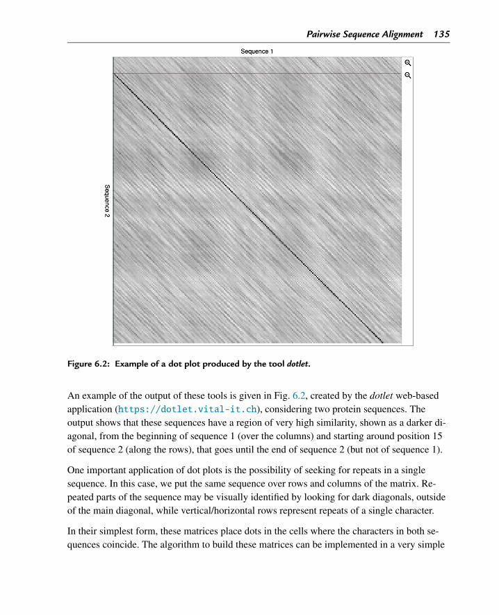
Pairwise Sequence Alignment 135

Figure 6.2: Example of a dot plot produced by the tool dotlet.

An example of the output of these tools is given in Fig. 6.2, created by the dotlet web-basedapplication (https://dotlet.vital-it.ch), considering two protein sequences. Theoutput shows that these sequences have a region of very high similarity, shown as a darker di-agonal, from the beginning of sequence 1 (over the columns) and starting around position 15of sequence 2 (along the rows), that goes until the end of sequence 2 (but not of sequence 1).

One important application of dot plots is the possibility of seeking for repeats in a singlesequence. In this case, we put the same sequence over rows and columns of the matrix. Re-peated parts of the sequence may be visually identified by looking for dark diagonals, outsideof the main diagonal, while vertical/horizontal rows represent repeats of a single character.

In their simplest form, these matrices place dots in the cells where the characters in both se-quences coincide. The algorithm to build these matrices can be implemented in a very simple

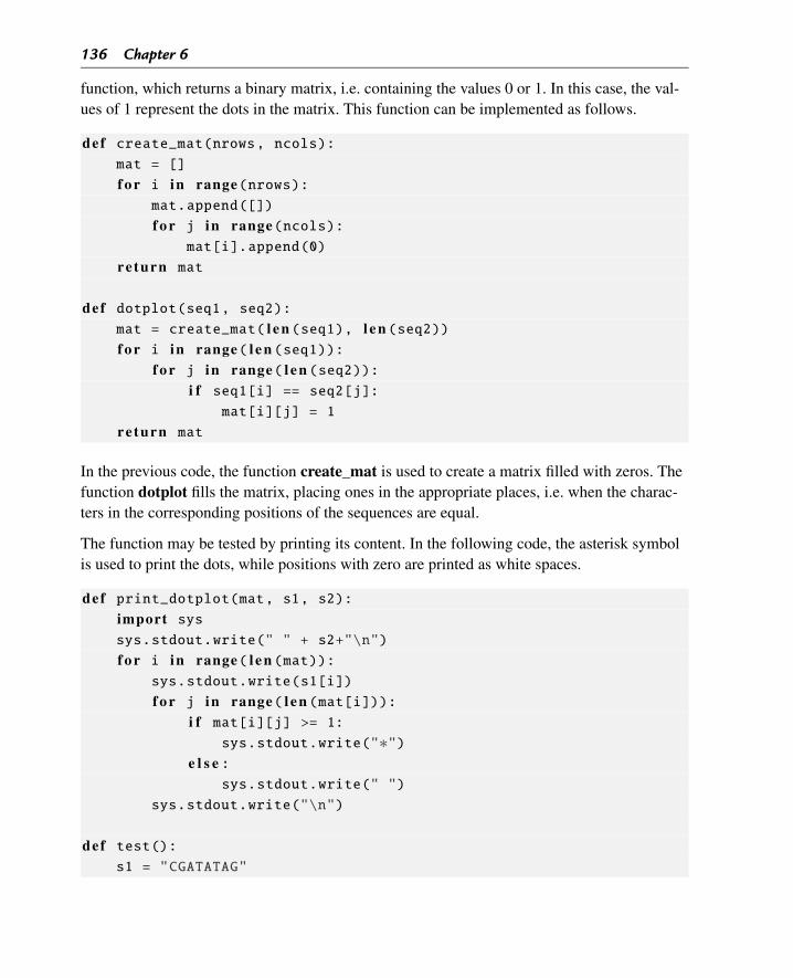
136 Chapter 6

function, which returns a binary matrix, i.e. containing the values 0 or 1. In this case, the val-ues of 1 represent the dots in the matrix. This function can be implemented as follows.

def create_mat(nrows, ncols):mat = []

f o r i in range(nrows):mat.append([])

f o r j in range(ncols):mat[i].append(0)

re turn mat

def dotplot(seq1, seq2):mat = create_mat( l e n (seq1), l e n (seq2))f o r i in range( l e n (seq1)):

f o r j in range( l e n (seq2)):i f seq1[i] == seq2[j]:

mat[i][j] = 1

re turn mat

In the previous code, the function create_mat is used to create a matrix filled with zeros. Thefunction dotplot fills the matrix, placing ones in the appropriate places, i.e. when the charac-ters in the corresponding positions of the sequences are equal.

The function may be tested by printing its content. In the following code, the asterisk symbolis used to print the dots, while positions with zero are printed as white spaces.

def print_dotplot(mat, s1, s2):import syssys.stdout.write(" " + s2+"\n")

f o r i in range( l e n (mat)):sys.stdout.write(s1[i])

f o r j in range( l e n (mat[i])):i f mat[i][j] >= 1:

sys.stdout.write("∗")e l s e :

sys.stdout.write(" ")

sys.stdout.write("\n")

def test():s1 = "CGATATAG"

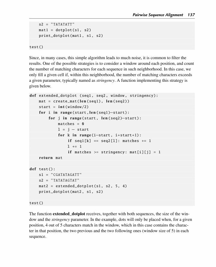
Pairwise Sequence Alignment 137

s2 = "TATATATT"

mat1 = dotplot(s1, s2)

print_dotplot(mat1, s1, s2)

test()

Since, in many cases, this simple algorithm leads to much noise, it is common to filter theresults. One of the possible strategies is to consider a window around each position, and countthe number of matching characters for each sequence in such neighborhood. In this case, weonly fill a given cell if, within this neighborhood, the number of matching characters exceedsa given parameter, typically named as stringency. A function implementing this strategy isgiven below.

def extended_dotplot (seq1, seq2, window, stringency):mat = create_mat( l e n (seq1), l e n (seq2))start = i n t (window/2)f o r i in range(start, l e n (seq1)−start):

f o r j in range(start, l e n (seq2)−start):matches = 0

l = j − start

f o r k in range(i−start, i+start+1):i f seq1[k] == seq2[l]: matches += 1l += 1

i f matches >= stringency: mat[i][j] = 1re turn mat

def test():s1 = "CGATATAGATT"

s2 = "TATATAGTAT"

mat2 = extended_dotplot(s1, s2, 5, 4)

print_dotplot(mat2, s1, s2)

test()

The function extended_dotplot receives, together with both sequences, the size of the win-dow and the stringency parameter. In the example, dots will only be placed when, for a givenposition, 4 out of 5 characters match in the window, which in this case contains the charac-ter in that position, the two previous and the two following ones (window size of 5) in eachsequence.

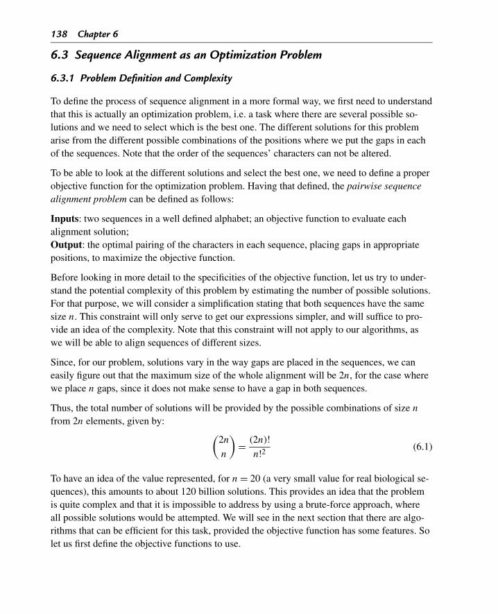
138 Chapter 6

6.3 Sequence Alignment as an Optimization Problem

6.3.1 Problem Definition and Complexity

To define the process of sequence alignment in a more formal way, we first need to understandthat this is actually an optimization problem, i.e. a task where there are several possible so-lutions and we need to select which is the best one. The different solutions for this problemarise from the different possible combinations of the positions where we put the gaps in eachof the sequences. Note that the order of the sequences’ characters can not be altered.

To be able to look at the different solutions and select the best one, we need to define a properobjective function for the optimization problem. Having that defined, the pairwise sequencealignment problem can be defined as follows:

Inputs: two sequences in a well defined alphabet; an objective function to evaluate eachalignment solution;Output: the optimal pairing of the characters in each sequence, placing gaps in appropriatepositions, to maximize the objective function.

Before looking in more detail to the specificities of the objective function, let us try to under-stand the potential complexity of this problem by estimating the number of possible solutions.For that purpose, we will consider a simplification stating that both sequences have the samesize n. This constraint will only serve to get our expressions simpler, and will suffice to pro-vide an idea of the complexity. Note that this constraint will not apply to our algorithms, aswe will be able to align sequences of different sizes.

Since, for our problem, solutions vary in the way gaps are placed in the sequences, we caneasily figure out that the maximum size of the whole alignment will be 2n, for the case wherewe place n gaps, since it does not make sense to have a gap in both sequences.

Thus, the total number of solutions will be provided by the possible combinations of size n

from 2n elements, given by: (2n

n

)= (2n)!

n!2 (6.1)

To have an idea of the value represented, for n = 20 (a very small value for real biological se-quences), this amounts to about 120 billion solutions. This provides an idea that the problemis quite complex and that it is impossible to address by using a brute-force approach, whereall possible solutions would be attempted. We will see in the next section that there are algo-rithms that can be efficient for this task, provided the objective function has some features. Solet us first define the objective functions to use.

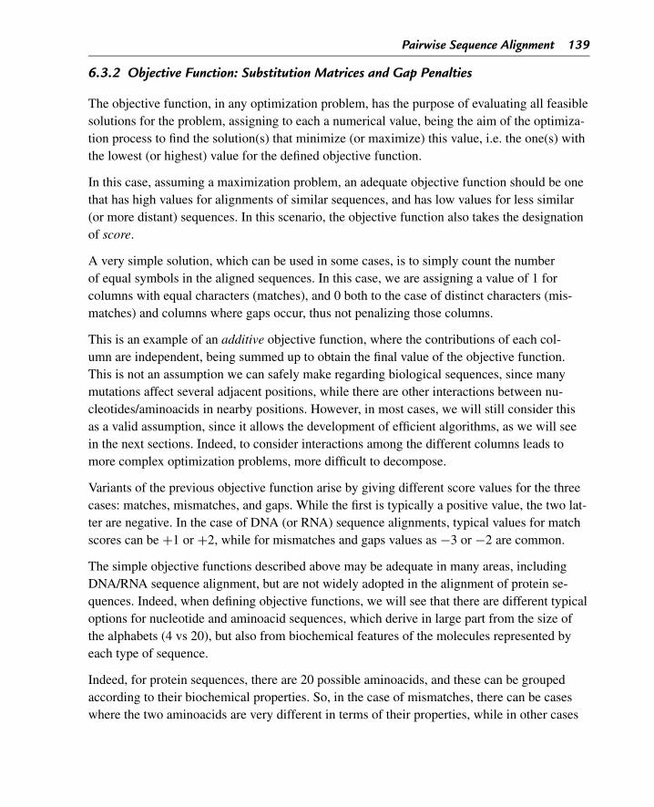
Pairwise Sequence Alignment 139

6.3.2 Objective Function: Substitution Matrices and Gap Penalties

The objective function, in any optimization problem, has the purpose of evaluating all feasiblesolutions for the problem, assigning to each a numerical value, being the aim of the optimiza-tion process to find the solution(s) that minimize (or maximize) this value, i.e. the one(s) withthe lowest (or highest) value for the defined objective function.

In this case, assuming a maximization problem, an adequate objective function should be onethat has high values for alignments of similar sequences, and has low values for less similar(or more distant) sequences. In this scenario, the objective function also takes the designationof score.

A very simple solution, which can be used in some cases, is to simply count the numberof equal symbols in the aligned sequences. In this case, we are assigning a value of 1 forcolumns with equal characters (matches), and 0 both to the case of distinct characters (mis-matches) and columns where gaps occur, thus not penalizing those columns.

This is an example of an additive objective function, where the contributions of each col-umn are independent, being summed up to obtain the final value of the objective function.This is not an assumption we can safely make regarding biological sequences, since manymutations affect several adjacent positions, while there are other interactions between nu-cleotides/aminoacids in nearby positions. However, in most cases, we will still consider thisas a valid assumption, since it allows the development of efficient algorithms, as we will seein the next sections. Indeed, to consider interactions among the different columns leads tomore complex optimization problems, more difficult to decompose.

Variants of the previous objective function arise by giving different score values for the threecases: matches, mismatches, and gaps. While the first is typically a positive value, the two lat-ter are negative. In the case of DNA (or RNA) sequence alignments, typical values for matchscores can be +1 or +2, while for mismatches and gaps values as −3 or −2 are common.

The simple objective functions described above may be adequate in many areas, includingDNA/RNA sequence alignment, but are not widely adopted in the alignment of protein se-quences. Indeed, when defining objective functions, we will see that there are different typicaloptions for nucleotide and aminoacid sequences, which derive in large part from the size ofthe alphabets (4 vs 20), but also from biochemical features of the molecules represented byeach type of sequence.

Indeed, for protein sequences, there are 20 possible aminoacids, and these can be groupedaccording to their biochemical properties. So, in the case of mismatches, there can be caseswhere the two aminoacids are very different in terms of their properties, while in other cases

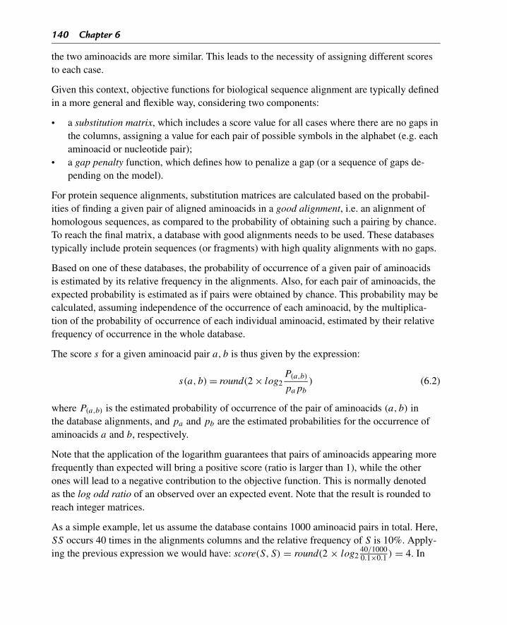
140 Chapter 6

the two aminoacids are more similar. This leads to the necessity of assigning different scoresto each case.

Given this context, objective functions for biological sequence alignment are typically definedin a more general and flexible way, considering two components:

• a substitution matrix, which includes a score value for all cases where there are no gaps inthe columns, assigning a value for each pair of possible symbols in the alphabet (e.g. eachaminoacid or nucleotide pair);

• a gap penalty function, which defines how to penalize a gap (or a sequence of gaps de-pending on the model).

For protein sequence alignments, substitution matrices are calculated based on the probabil-ities of finding a given pair of aligned aminoacids in a good alignment, i.e. an alignment ofhomologous sequences, as compared to the probability of obtaining such a pairing by chance.To reach the final matrix, a database with good alignments needs to be used. These databasestypically include protein sequences (or fragments) with high quality alignments with no gaps.

Based on one of these databases, the probability of occurrence of a given pair of aminoacidsis estimated by its relative frequency in the alignments. Also, for each pair of aminoacids, theexpected probability is estimated as if pairs were obtained by chance. This probability may becalculated, assuming independence of the occurrence of each aminoacid, by the multiplica-tion of the probability of occurrence of each individual aminoacid, estimated by their relativefrequency of occurrence in the whole database.

The score s for a given aminoacid pair a, b is thus given by the expression:

s(a, b) = round(2 × log2P(a,b)

papb

) (6.2)

where P(a,b) is the estimated probability of occurrence of the pair of aminoacids (a, b) inthe database alignments, and pa and pb are the estimated probabilities for the occurrence ofaminoacids a and b, respectively.

Note that the application of the logarithm guarantees that pairs of aminoacids appearing morefrequently than expected will bring a positive score (ratio is larger than 1), while the otherones will lead to a negative contribution to the objective function. This is normally denotedas the log odd ratio of an observed over an expected event. Note that the result is rounded toreach integer matrices.

As a simple example, let us assume the database contains 1000 aminoacid pairs in total. Here,SS occurs 40 times in the alignments columns and the relative frequency of S is 10%. Apply-ing the previous expression we would have: score(S, S) = round(2 × log2

40/10000.1×0.1 ) = 4. In

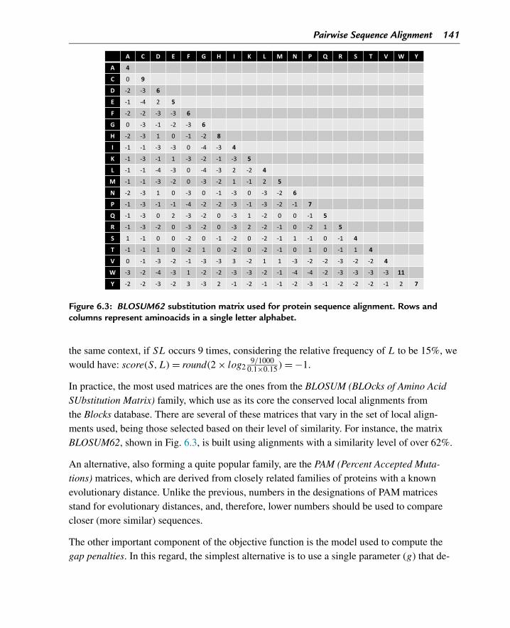
Pairwise Sequence Alignment 141

Figure 6.3: BLOSUM62 substitution matrix used for protein sequence alignment. Rows andcolumns represent aminoacids in a single letter alphabet.

the same context, if SL occurs 9 times, considering the relative frequency of L to be 15%, wewould have: score(S,L) = round(2 × log2

9/10000.1×0.15 ) = −1.

In practice, the most used matrices are the ones from the BLOSUM (BLOcks of Amino AcidSUbstitution Matrix) family, which use as its core the conserved local alignments fromthe Blocks database. There are several of these matrices that vary in the set of local align-ments used, being those selected based on their level of similarity. For instance, the matrixBLOSUM62, shown in Fig. 6.3, is built using alignments with a similarity level of over 62%.

An alternative, also forming a quite popular family, are the PAM (Percent Accepted Muta-tions) matrices, which are derived from closely related families of proteins with a knownevolutionary distance. Unlike the previous, numbers in the designations of PAM matricesstand for evolutionary distances, and, therefore, lower numbers should be used to comparecloser (more similar) sequences.

The other important component of the objective function is the model used to compute thegap penalties. In this regard, the simplest alternative is to use a single parameter (g) that de-

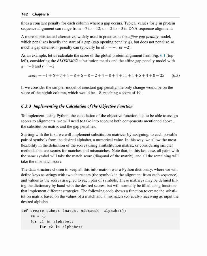
142 Chapter 6

fines a constant penalty for each column where a gap occurs. Typical values for g in proteinsequence alignment can range from −7 to −12, or −2 to −3 in DNA sequence alignment.

A more sophisticated alternative, widely used in practice, is the affine gap penalty model,which penalizes heavily the start of a gap (gap opening penalty g), but does not penalize somuch a gap extension (penalty can typically be of r = −1 or −2).

As an example, let us calculate the score of the global protein alignment from Fig. 6.1 (topleft), considering the BLOSUM62 substitution matrix and the affine gap penalty model withg = −8 and r = −2:

score = −1 + 6 + 7 + 4 − 8 + 6 − 8 − 2 + 4 − 8 + 4 + 11 + 1 + 5 + 4 + 0 = 25 (6.3)

If we consider the simpler model of constant gap penalty, the only change would be on thescore of the eighth column, which would be −8, reaching a score of 19.

6.3.3 Implementing the Calculation of the Objective Function

To implement, using Python, the calculation of the objective function, i.e. to be able to assignscores to alignments, we will need to take into account both components mentioned above,the substitution matrix and the gap penalties.

Starting with the first, we will implement substitution matrices by assigning, to each possiblepair of symbols from the desired alphabet, a numerical value. In this way, we allow the mostflexibility in the definition of the scores using a substitution matrix, or considering simplermethods that use scores for matches and mismatches. Note that, in this last case, all pairs withthe same symbol will take the match score (diagonal of the matrix), and all the remaining willtake the mismatch score.

The data structure chosen to keep all this information was a Python dictionary, where we willdefine keys as strings with two characters (the symbols in the alignment from each sequence),and values as the scores assigned to each pair of symbols. These matrices may be defined fill-ing the dictionary by hand with the desired scores, but will normally be filled using functionsthat implement different strategies. The following code shows a function to create the substi-tution matrix based on the values of a match and a mismatch score, also receiving as input thedesired alphabet.

def create_submat (match, mismatch, alphabet):sm = {}

f o r c1 in alphabet:

f o r c2 in alphabet:

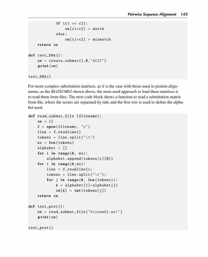
Pairwise Sequence Alignment 143

i f (c1 == c2):sm[c1+c2] = match

e l s e :sm[c1+c2] = mismatch

re turn sm

def test_DNA():sm = create_submat(1,0,"ACGT")

p r i n t (sm)

test_DNA()

For more complex substitution matrices, as it is the case with those used in protein align-ments, as the BLOSUM62 shown above, the most used approach to load these matrices isto read them from files. The next code block shows a function to read a substitution matrixfrom file, where the scores are separated by tabs and the first row is used to define the alpha-bet used.

def read_submat_file (filename):sm = {}

f = open(filename, "r")line = f.readline()

tokens = line.split("\t")

ns = l e n (tokens)alphabet = []

f o r i in range(0, ns):alphabet.append(tokens[i][0])

f o r i in range(0,ns):line = f.readline();

tokens = line.split("\t");

f o r j in range(0, l e n (tokens)):k = alphabet[i]+alphabet[j]

sm[k] = i n t (tokens[j])re turn sm

def test_prot():sm = read_submat_file("blosum62.mat")

p r i n t (sm)

test_prot()

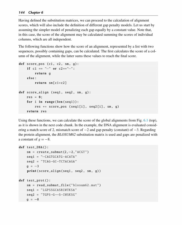
144 Chapter 6

Having defined the substitution matrices, we can proceed to the calculation of alignmentscores, which will also include the definition of different gap penalty models. Let us start byassuming the simpler model of penalizing each gap equally by a constant value. Note that,in this case, the score of the alignment may be calculated summing the scores of individualcolumns, which are all independent.

The following functions show how the score of an alignment, represented by a list with twosequences, possibly containing gaps, can be calculated. The first calculates the score of a col-umn of the alignment, while the latter sums these values to reach the final score.

def score_pos (c1, c2, sm, g):i f c1 == "−" or c2=="−":

re turn ge l s e :

re turn sm[c1+c2]

def score_align (seq1, seq2, sm, g):res = 0;

f o r i in range( l e n (seq1)):res += score_pos (seq1[i], seq2[i], sm, g)

re turn res

Using these functions, we can calculate the score of the global alignments from Fig. 6.1 (top),as it is shown in the next code chunk. In the example, the DNA alignment is evaluated consid-ering a match score of 2, mismatch score of −2 and gap penalty (constant) of −3. Regardingthe protein alignment, the BLOSUM62 substitution matrix is used and gaps are penalized witha constant of g = −8.

def test_DNA():sm = create_submat(2,−2,"ACGT")seq1 = "−CAGTGCATG−ACATA"seq2 = "TCAG−GC−TCTACAGA"g = −3p r i n t (score_align(seq1, seq2, sm, g))

def test_prot():sm = read_submat_file("blosum62.mat")

seq1 = "LGPSSGCASRIWTKSA"

seq2 = "TGPS−G−−S−IWSKSG"g = −8

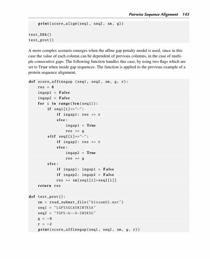
Pairwise Sequence Alignment 145

p r i n t (score_align(seq1, seq2, sm, g))

test_DNA()

test_prot()

A more complex scenario emerges when the affine gap penalty model is used, since in thiscase the value of each column can be dependent of previous columns, in the case of multi-ple consecutive gaps. The following function handles this case, by using two flags which areset to True when inside gap sequences. The function is applied to the previous example of aprotein sequence alignment.

def score_affinegap (seq1, seq2, sm, g, r):res = 0

ingap1 = F a l s eingap2 = F a l s ef o r i in range( l e n (seq1)):

i f seq1[i]=="−":i f ingap1: res += re l s e :

ingap1 = Trueres += g

e l i f seq2[i]=="−":i f ingap2: res += re l s e :

ingap2 = Trueres += g

e l s e :i f ingap1: ingap1 = F a l s ei f ingap2: ingap2 = F a l s eres += sm[seq1[i]+seq2[i]]

re turn res

def test_prot():sm = read_submat_file("blosum62.mat")

seq1 = "LGPSSGCASRIWTKSA"

seq2 = "TGPS−G−−S−IWSKSG"g = −8r = −2p r i n t (score_affinegap(seq1, seq2, sm, g, r))

146 Chapter 6

test_prot()

6.4 Dynamic Programming Algorithms for Global Alignment

6.4.1 The Needleman-Wunsch Algorithm

We have already realized that the pairwise sequence alignment problem is quite complexwith a huge number of possible solutions, even for moderate sized sequences. Since we donot have the possibility of trying all possible solutions, we need to find more intelligent ap-proaches for the problem.

The main idea driving these algorithms will be a divide-and-conquer approach, quite commonto address complex problems by sub-dividing those into simpler problems and combiningtheir solutions. This is made possible by the additive nature of the scoring functions we havepresented in the previous section, which allows to decompose a solution (an alignment) on itsdifferent columns, being the overall score the sum of the scores of the columns.

Notice that the affine gap penalty assumption does not obey this principle, and, therefore, thealgorithms we will study in these sections will consider the simpler gap penalty based on aconstant per gap (column). It is still possible to define similar algorithms for the affine gappenalty model, but these are more complex and will not be covered in this text.

Based on these observations, in the early days of Bioinformatics, different researchers haveproposed the use of dynamic programming (DP) algorithms to address biological sequencealignment. DP is a general-purpose class of optimization algorithms based on a divide-and-conquer approach, where optimal solutions for sub-problems and their scores are re-used (andnot recomputed) when solving larger problems. This idea has been applied to sequence align-ment considering that the alignment of two sequences can be composed from alignments ofsub-sequences of those sequences.

We will next detail these algorithms, starting with the Needleman-Wunsch (NW) algorithmfor global sequence alignment, whose name is derived from the two authors that proposed it.Consider we want to align two sequences A and B of sizes n and m, respectively. The indi-vidual symbols in A and B can be accessed by subscripting, using indexes, and thus we canrepresent A = a1a2 . . . an and B = b1b2 . . . bm.

When executing the NW algorithm, we will build a matrix S, where the elements of se-quence A will be placed to index rows and the elements of sequence B will be placed to indexcolumns. We will add an extra column and an extra row in the beginning to represent align-ments with gaps in all positions of one of the sequences.

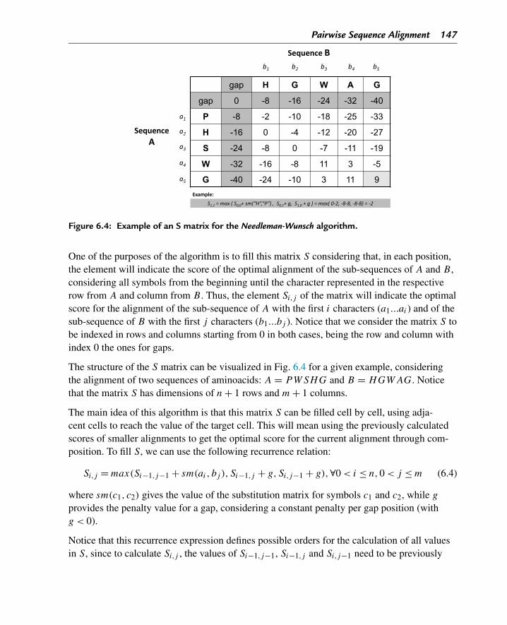
Pairwise Sequence Alignment 147

Figure 6.4: Example of an S matrix for the Needleman-Wunsch algorithm.

One of the purposes of the algorithm is to fill this matrix S considering that, in each position,the element will indicate the score of the optimal alignment of the sub-sequences of A and B ,considering all symbols from the beginning until the character represented in the respectiverow from A and column from B . Thus, the element Si,j of the matrix will indicate the optimalscore for the alignment of the sub-sequence of A with the first i characters (a1...ai ) and of thesub-sequence of B with the first j characters (b1...bj ). Notice that we consider the matrix S tobe indexed in rows and columns starting from 0 in both cases, being the row and column withindex 0 the ones for gaps.

The structure of the S matrix can be visualized in Fig. 6.4 for a given example, consideringthe alignment of two sequences of aminoacids: A = PWSHG and B = HGWAG. Noticethat the matrix S has dimensions of n + 1 rows and m + 1 columns.

The main idea of this algorithm is that this matrix S can be filled cell by cell, using adja-cent cells to reach the value of the target cell. This will mean using the previously calculatedscores of smaller alignments to get the optimal score for the current alignment through com-position. To fill S, we can use the following recurrence relation:

Si,j = max(Si−1,j−1 + sm(ai, bj ), Si−1,j + g,Si,j−1 + g),∀0 < i ≤ n,0 < j ≤ m (6.4)

where sm(c1, c2) gives the value of the substitution matrix for symbols c1 and c2, while g

provides the penalty value for a gap, considering a constant penalty per gap position (withg < 0).

Notice that this recurrence expression defines possible orders for the calculation of all valuesin S, since to calculate Si,j , the values of Si−1,j−1, Si−1,j and Si,j−1 need to be previously

148 Chapter 6

known. In practice, we fill the matrix by rows or by columns going from left to right and fromtop to bottom, i.e. increasing the indexes.

This recurrence relation states that an alignment may always be obtained by the compositionof other alignments. In particular, it builds an alignment by adding an extra column to a previ-ous alignment and computing the new score by summing the previous score with the one fromthe added column.

There are three ways to add a column to a previous alignment: to add a column with the nextsymbols from each sequence, to add the next symbol from the first sequence and a gap, orto add the next symbol from the second sequence and a gap. These are the three hypothesesgiven in the recurrence from Eq. (6.4). In the first hypothesis, the score of the new columnis calculated by checking the respective entry in the substitution matrix, while in the othertwo the score is given by g. The new scores are added to the previous ones and the maximumscore is taken for the new alignment and used to fill S in that position.

To fill S using this recurrence relation, we need to define how to initialize the matrix, fillingthe first row and the first column. In both cases, the idea will be to multiply the number ofcolumns in the alignment by g, since these alignments are composed of only gaps in one ofthe sequences. Thus, Si,0 = i ∗ g, ∀0 < i ≤ n and S0,j = j ∗ g, ∀0 < j ≤ m.

Fig. 6.4 provides an example of the application of the algorithm to fill S. In this case, the sub-stitution matrix used is the BLOSUM62 provided in Fig. 6.3 and g = −8.

Notice that, in example from the figure, the gaps’ row and column are shaded gray beingcalculated as stated above. For the remaining cells, the recurrence relation from Eq. (6.4) isapplied. An example is provided in the figure for the cell S1,1.

From the definition put forward for the matrix S, it is easy to conclude that the overall scoreof the best alignment, for the whole sequences, is given in the lower right corner of the matrix(cell highlighted with dots in the figure).

The process explained above allows to reach the score for the optimal alignment (indeed forall optimal alignments of sub-sequences from the original sequences starting at the first posi-tion), but it is still not sufficient to obtain the best alignment itself. To be able to reconstructthe best alignment, we need to “memorize” the decisions took every time the recurrence re-lation is applied. Indeed, we need to store the information of which was the hypothesis (fromthe three possible ones) that provided the highest score, and consequently which was the pre-vious alignment.

This is normally achieved by encoding these choices using a 3 symbol alphabet and building atrace-back matrix, typically denoted as T , with the same dimensions as the S matrix. Fig. 6.5

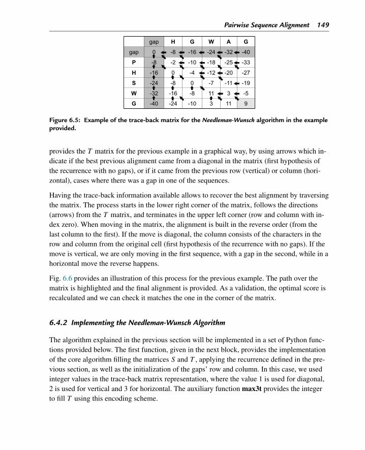
Pairwise Sequence Alignment 149

Figure 6.5: Example of the trace-back matrix for the Needleman-Wunsch algorithm in the exampleprovided.

provides the T matrix for the previous example in a graphical way, by using arrows which in-dicate if the best previous alignment came from a diagonal in the matrix (first hypothesis ofthe recurrence with no gaps), or if it came from the previous row (vertical) or column (hori-zontal), cases where there was a gap in one of the sequences.

Having the trace-back information available allows to recover the best alignment by traversingthe matrix. The process starts in the lower right corner of the matrix, follows the directions(arrows) from the T matrix, and terminates in the upper left corner (row and column with in-dex zero). When moving in the matrix, the alignment is built in the reverse order (from thelast column to the first). If the move is diagonal, the column consists of the characters in therow and column from the original cell (first hypothesis of the recurrence with no gaps). If themove is vertical, we are only moving in the first sequence, with a gap in the second, while in ahorizontal move the reverse happens.

Fig. 6.6 provides an illustration of this process for the previous example. The path over thematrix is highlighted and the final alignment is provided. As a validation, the optimal score isrecalculated and we can check it matches the one in the corner of the matrix.

6.4.2 Implementing the Needleman-Wunsch Algorithm

The algorithm explained in the previous section will be implemented in a set of Python func-tions provided below. The first function, given in the next block, provides the implementationof the core algorithm filling the matrices S and T , applying the recurrence defined in the pre-vious section, as well as the initialization of the gaps’ row and column. In this case, we usedinteger values in the trace-back matrix representation, where the value 1 is used for diagonal,2 is used for vertical and 3 for horizontal. The auxiliary function max3t provides the integerto fill T using this encoding scheme.

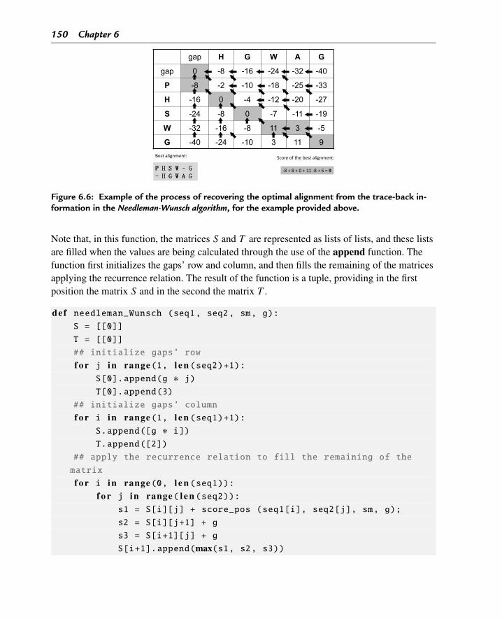
150 Chapter 6

Figure 6.6: Example of the process of recovering the optimal alignment from the trace-back in-formation in the Needleman-Wunsch algorithm, for the example provided above.

Note that, in this function, the matrices S and T are represented as lists of lists, and these listsare filled when the values are being calculated through the use of the append function. Thefunction first initializes the gaps’ row and column, and then fills the remaining of the matricesapplying the recurrence relation. The result of the function is a tuple, providing in the firstposition the matrix S and in the second the matrix T .

def needleman_Wunsch (seq1, seq2, sm, g):S = [[0]]

T = [[0]]

## initialize gaps’ row

f o r j in range(1, l e n (seq2)+1):S[0].append(g ∗ j)T[0].append(3)

## initialize gaps’ column

f o r i in range(1, l e n (seq1)+1):S.append([g ∗ i])T.append([2])

## apply the recurrence relation to fill the remaining of the

matrix

f o r i in range(0, l e n (seq1)):f o r j in range( l e n (seq2)):

s1 = S[i][j] + score_pos (seq1[i], seq2[j], sm, g);

s2 = S[i][j+1] + g

s3 = S[i+1][j] + g

S[i+1].append(max(s1, s2, s3))

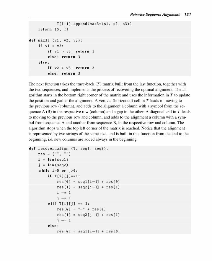
Pairwise Sequence Alignment 151

T[i+1].append(max3t(s1, s2, s3))

re turn (S, T)

def max3t (v1, v2, v3):i f v1 > v2:

i f v1 > v3: re turn 1e l s e : re turn 3

e l s e :i f v2 > v3: re turn 2e l s e : re turn 3

The next function takes the trace-back (T ) matrix built from the last function, together withthe two sequences, and implements the process of recovering the optimal alignment. The al-gorithm starts in the bottom right corner of the matrix and uses the information in T to updatethe position and gather the alignment. A vertical (horizontal) cell in T leads to moving tothe previous row (column), and adds to the alignment a column with a symbol from the se-quence A (B) in the respective row (column) and a gap in the other. A diagonal cell in T leadsto moving to the previous row and column, and adds to the alignment a column with a sym-bol from sequence A and another from sequence B, in the respective row and column. Thealgorithm stops when the top left corner of the matrix is reached. Notice that the alignmentis represented by two strings of the same size, and is built in this function from the end to thebeginning, i.e. new columns are added always in the beginning.

def recover_align (T, seq1, seq2):res = ["", ""]

i = l e n (seq1)j = l e n (seq2)whi le i>0 or j>0:

i f T[i][j]==1:res[0] = seq1[i−1] + res[0]res[1] = seq2[j−1] + res[1]i −= 1j −= 1

e l i f T[i][j] == 3:res[0] = "−" + res[0]res[1] = seq2[j−1] + res[1]j −= 1

e l s e :res[0] = seq1[i−1] + res[0]

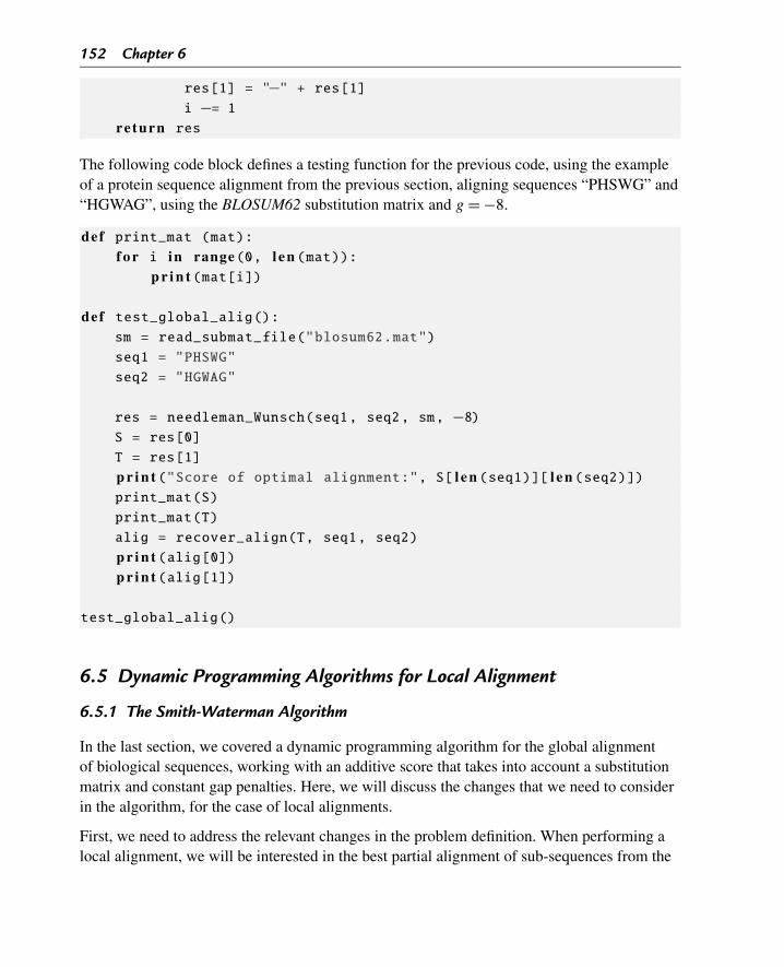
152 Chapter 6

res[1] = "−" + res[1]i −= 1

re turn res

The following code block defines a testing function for the previous code, using the exampleof a protein sequence alignment from the previous section, aligning sequences “PHSWG” and“HGWAG”, using the BLOSUM62 substitution matrix and g = −8.

def print_mat (mat):f o r i in range(0, l e n (mat)):

p r i n t (mat[i])

def test_global_alig():sm = read_submat_file("blosum62.mat")

seq1 = "PHSWG"

seq2 = "HGWAG"

res = needleman_Wunsch(seq1, seq2, sm, −8)S = res[0]

T = res[1]

p r i n t ("Score of optimal alignment:", S[ l e n (seq1)][ l e n (seq2)])print_mat(S)

print_mat(T)

alig = recover_align(T, seq1, seq2)

p r i n t (alig[0])p r i n t (alig[1])

test_global_alig()

6.5 Dynamic Programming Algorithms for Local Alignment

6.5.1 The Smith-Waterman Algorithm

In the last section, we covered a dynamic programming algorithm for the global alignmentof biological sequences, working with an additive score that takes into account a substitutionmatrix and constant gap penalties. Here, we will discuss the changes that we need to considerin the algorithm, for the case of local alignments.

First, we need to address the relevant changes in the problem definition. When performing alocal alignment, we will be interested in the best partial alignment of sub-sequences from the

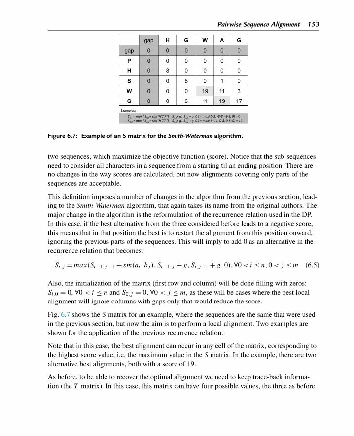
Pairwise Sequence Alignment 153

Figure 6.7: Example of an S matrix for the Smith-Waterman algorithm.

two sequences, which maximize the objective function (score). Notice that the sub-sequencesneed to consider all characters in a sequence from a starting til an ending position. There areno changes in the way scores are calculated, but now alignments covering only parts of thesequences are acceptable.

This definition imposes a number of changes in the algorithm from the previous section, lead-ing to the Smith-Waterman algorithm, that again takes its name from the original authors. Themajor change in the algorithm is the reformulation of the recurrence relation used in the DP.In this case, if the best alternative from the three considered before leads to a negative score,this means that in that position the best is to restart the alignment from this position onward,ignoring the previous parts of the sequences. This will imply to add 0 as an alternative in therecurrence relation that becomes:

Si,j = max(Si−1,j−1 + sm(ai, bj ), Si−1,j + g,Si,j−1 + g,0),∀0 < i ≤ n,0 < j ≤ m (6.5)

Also, the initialization of the matrix (first row and column) will be done filling with zeros:Si,0 = 0, ∀0 < i ≤ n and S0,j = 0, ∀0 < j ≤ m, as these will be cases where the best localalignment will ignore columns with gaps only that would reduce the score.

Fig. 6.7 shows the S matrix for an example, where the sequences are the same that were usedin the previous section, but now the aim is to perform a local alignment. Two examples areshown for the application of the previous recurrence relation.

Note that in this case, the best alignment can occur in any cell of the matrix, corresponding tothe highest score value, i.e. the maximum value in the S matrix. In the example, there are twoalternative best alignments, both with a score of 19.

As before, to be able to recover the optimal alignment we need to keep trace-back informa-tion (the T matrix). In this case, this matrix can have four possible values, the three as before

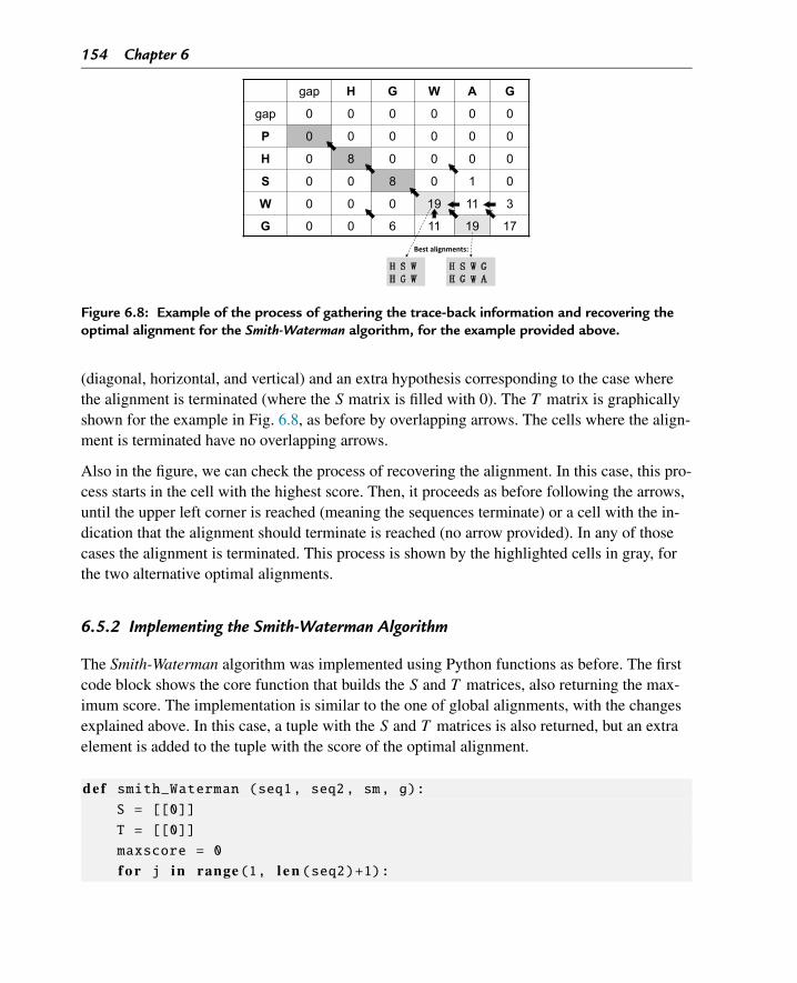
154 Chapter 6

Figure 6.8: Example of the process of gathering the trace-back information and recovering theoptimal alignment for the Smith-Waterman algorithm, for the example provided above.

(diagonal, horizontal, and vertical) and an extra hypothesis corresponding to the case wherethe alignment is terminated (where the S matrix is filled with 0). The T matrix is graphicallyshown for the example in Fig. 6.8, as before by overlapping arrows. The cells where the align-ment is terminated have no overlapping arrows.

Also in the figure, we can check the process of recovering the alignment. In this case, this pro-cess starts in the cell with the highest score. Then, it proceeds as before following the arrows,until the upper left corner is reached (meaning the sequences terminate) or a cell with the in-dication that the alignment should terminate is reached (no arrow provided). In any of thosecases the alignment is terminated. This process is shown by the highlighted cells in gray, forthe two alternative optimal alignments.

6.5.2 Implementing the Smith-Waterman Algorithm

The Smith-Waterman algorithm was implemented using Python functions as before. The firstcode block shows the core function that builds the S and T matrices, also returning the max-imum score. The implementation is similar to the one of global alignments, with the changesexplained above. In this case, a tuple with the S and T matrices is also returned, but an extraelement is added to the tuple with the score of the optimal alignment.

def smith_Waterman (seq1, seq2, sm, g):S = [[0]]

T = [[0]]

maxscore = 0

f o r j in range(1, l e n (seq2)+1):

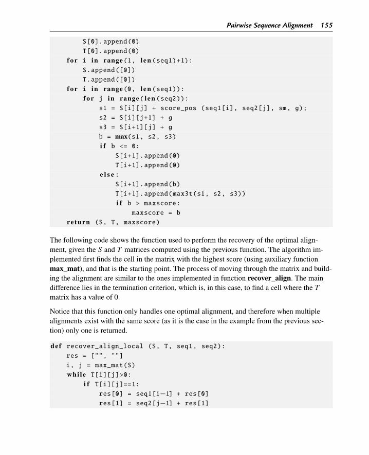
Pairwise Sequence Alignment 155

S[0].append(0)

T[0].append(0)

f o r i in range(1, l e n (seq1)+1):S.append([0])

T.append([0])

f o r i in range(0, l e n (seq1)):f o r j in range( l e n (seq2)):

s1 = S[i][j] + score_pos (seq1[i], seq2[j], sm, g);

s2 = S[i][j+1] + g

s3 = S[i+1][j] + g

b = max(s1, s2, s3)i f b <= 0:

S[i+1].append(0)

T[i+1].append(0)

e l s e :S[i+1].append(b)

T[i+1].append(max3t(s1, s2, s3))

i f b > maxscore:maxscore = b

re turn (S, T, maxscore)

The following code shows the function used to perform the recovery of the optimal align-ment, given the S and T matrices computed using the previous function. The algorithm im-plemented first finds the cell in the matrix with the highest score (using auxiliary functionmax_mat), and that is the starting point. The process of moving through the matrix and build-ing the alignment are similar to the ones implemented in function recover_align. The maindifference lies in the termination criterion, which is, in this case, to find a cell where the T

matrix has a value of 0.

Notice that this function only handles one optimal alignment, and therefore when multiplealignments exist with the same score (as it is the case in the example from the previous sec-tion) only one is returned.

def recover_align_local (S, T, seq1, seq2):res = ["", ""]

i, j = max_mat(S)

whi le T[i][j]>0:i f T[i][j]==1:

res[0] = seq1[i−1] + res[0]res[1] = seq2[j−1] + res[1]

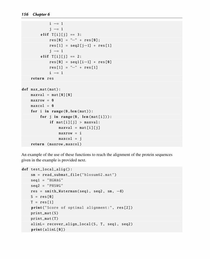
156 Chapter 6

i −= 1j −= 1

e l i f T[i][j] == 3:res[0] = "−" + res[0];res[1] = seq2[j−1] + res[1]j −= 1

e l i f T[i][j] == 2:res[0] = seq1[i−1] + res[0]res[1] = "−" + res[1]i −= 1

re turn res

def max_mat(mat):maxval = mat[0][0]

maxrow = 0

maxcol = 0

f o r i in range(0, l e n (mat)):f o r j in range(0, l e n (mat[i])):

i f mat[i][j] > maxval:maxval = mat[i][j]

maxrow = i

maxcol = j

re turn (maxrow,maxcol)

An example of the use of these functions to reach the alignment of the protein sequencesgiven in the example is provided next.

def test_local_alig():sm = read_submat_file("blosum62.mat")

seq1 = "HGWAG"

seq2 = "PHSWG"

res = smith_Waterman(seq1, seq2, sm, −8)S = res[0]

T = res[1]

p r i n t ("Score of optimal alignment:", res[2])print_mat(S)

print_mat(T)

alinL= recover_align_local(S, T, seq1, seq2)

p r i n t (alinL[0])

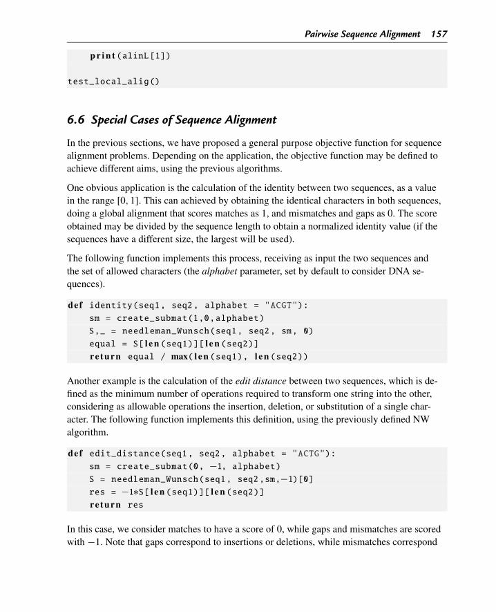
Pairwise Sequence Alignment 157

p r i n t (alinL[1])

test_local_alig()

6.6 Special Cases of Sequence Alignment

In the previous sections, we have proposed a general purpose objective function for sequencealignment problems. Depending on the application, the objective function may be defined toachieve different aims, using the previous algorithms.

One obvious application is the calculation of the identity between two sequences, as a valuein the range [0,1]. This can achieved by obtaining the identical characters in both sequences,doing a global alignment that scores matches as 1, and mismatches and gaps as 0. The scoreobtained may be divided by the sequence length to obtain a normalized identity value (if thesequences have a different size, the largest will be used).

The following function implements this process, receiving as input the two sequences andthe set of allowed characters (the alphabet parameter, set by default to consider DNA se-quences).

def identity(seq1, seq2, alphabet = "ACGT"):sm = create_submat(1,0,alphabet)

S,_ = needleman_Wunsch(seq1, seq2, sm, 0)

equal = S[ l e n (seq1)][ l e n (seq2)]re turn equal / max( l e n (seq1), l e n (seq2))

Another example is the calculation of the edit distance between two sequences, which is de-fined as the minimum number of operations required to transform one string into the other,considering as allowable operations the insertion, deletion, or substitution of a single char-acter. The following function implements this definition, using the previously defined NWalgorithm.

def edit_distance(seq1, seq2, alphabet = "ACTG"):sm = create_submat(0, −1, alphabet)S = needleman_Wunsch(seq1, seq2,sm,−1)[0]res = −1∗S[ l e n (seq1)][ l e n (seq2)]re turn res

In this case, we consider matches to have a score of 0, while gaps and mismatches are scoredwith −1. Note that gaps correspond to insertions or deletions, while mismatches correspond

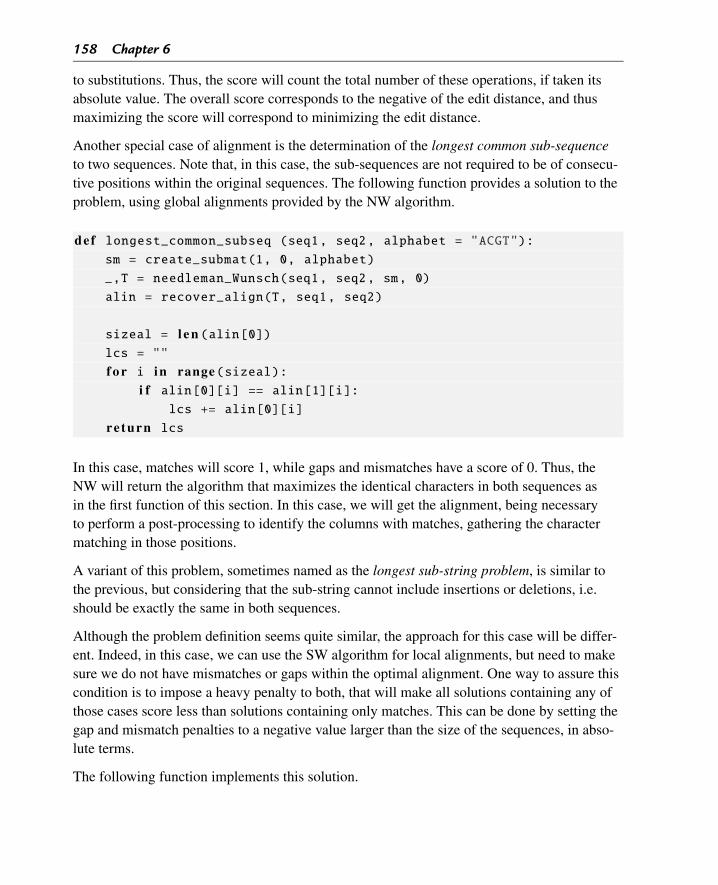
158 Chapter 6

to substitutions. Thus, the score will count the total number of these operations, if taken itsabsolute value. The overall score corresponds to the negative of the edit distance, and thusmaximizing the score will correspond to minimizing the edit distance.

Another special case of alignment is the determination of the longest common sub-sequenceto two sequences. Note that, in this case, the sub-sequences are not required to be of consecu-tive positions within the original sequences. The following function provides a solution to theproblem, using global alignments provided by the NW algorithm.

def longest_common_subseq (seq1, seq2, alphabet = "ACGT"):sm = create_submat(1, 0, alphabet)

_,T = needleman_Wunsch(seq1, seq2, sm, 0)

alin = recover_align(T, seq1, seq2)

sizeal = l e n (alin[0])lcs = ""

f o r i in range(sizeal):i f alin[0][i] == alin[1][i]:

lcs += alin[0][i]

re turn lcs

In this case, matches will score 1, while gaps and mismatches have a score of 0. Thus, theNW will return the algorithm that maximizes the identical characters in both sequences asin the first function of this section. In this case, we will get the alignment, being necessaryto perform a post-processing to identify the columns with matches, gathering the charactermatching in those positions.

A variant of this problem, sometimes named as the longest sub-string problem, is similar tothe previous, but considering that the sub-string cannot include insertions or deletions, i.e.should be exactly the same in both sequences.

Although the problem definition seems quite similar, the approach for this case will be differ-ent. Indeed, in this case, we can use the SW algorithm for local alignments, but need to makesure we do not have mismatches or gaps within the optimal alignment. One way to assure thiscondition is to impose a heavy penalty to both, that will make all solutions containing any ofthose cases score less than solutions containing only matches. This can be done by setting thegap and mismatch penalties to a negative value larger than the size of the sequences, in abso-lute terms.

The following function implements this solution.

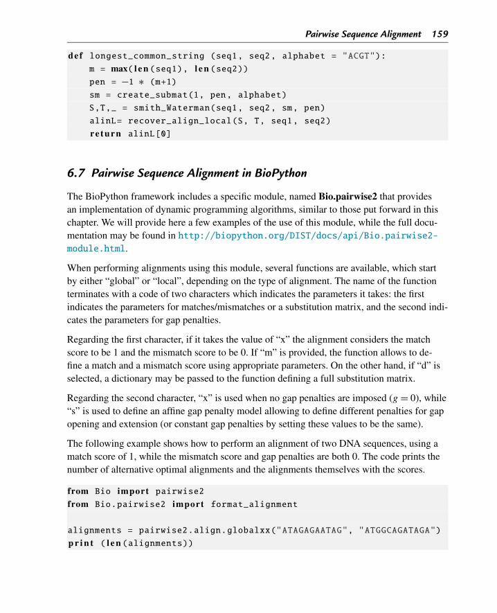
Pairwise Sequence Alignment 159

def longest_common_string (seq1, seq2, alphabet = "ACGT"):m = max( l e n (seq1), l e n (seq2))pen = −1 ∗ (m+1)sm = create_submat(1, pen, alphabet)

S,T,_ = smith_Waterman(seq1, seq2, sm, pen)

alinL= recover_align_local(S, T, seq1, seq2)

re turn alinL[0]

6.7 Pairwise Sequence Alignment in BioPython

The BioPython framework includes a specific module, named Bio.pairwise2 that providesan implementation of dynamic programming algorithms, similar to those put forward in thischapter. We will provide here a few examples of the use of this module, while the full docu-mentation may be found in http://biopython.org/DIST/docs/api/Bio.pairwise2-module.html.

When performing alignments using this module, several functions are available, which startby either “global” or “local”, depending on the type of alignment. The name of the functionterminates with a code of two characters which indicates the parameters it takes: the firstindicates the parameters for matches/mismatches or a substitution matrix, and the second indi-cates the parameters for gap penalties.

Regarding the first character, if it takes the value of “x” the alignment considers the matchscore to be 1 and the mismatch score to be 0. If “m” is provided, the function allows to de-fine a match and a mismatch score using appropriate parameters. On the other hand, if “d” isselected, a dictionary may be passed to the function defining a full substitution matrix.

Regarding the second character, “x” is used when no gap penalties are imposed (g = 0), while“s” is used to define an affine gap penalty model allowing to define different penalties for gapopening and extension (or constant gap penalties by setting these values to be the same).

The following example shows how to perform an alignment of two DNA sequences, using amatch score of 1, while the mismatch score and gap penalties are both 0. The code prints thenumber of alternative optimal alignments and the alignments themselves with the scores.

from Bio import pairwise2from Bio.pairwise2 import format_alignment

alignments = pairwise2.align.globalxx("ATAGAGAATAG", "ATGGCAGATAGA")

p r i n t ( l e n (alignments))

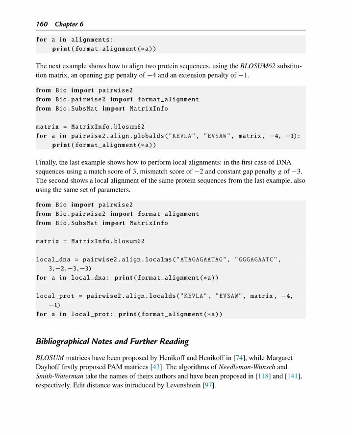
160 Chapter 6

f o r a in alignments:

p r i n t (format_alignment(∗a))

The next example shows how to align two protein sequences, using the BLOSUM62 substitu-tion matrix, an opening gap penalty of −4 and an extension penalty of −1.

from Bio import pairwise2from Bio.pairwise2 import format_alignmentfrom Bio.SubsMat import MatrixInfo

matrix = MatrixInfo.blosum62

f o r a in pairwise2.align.globalds("KEVLA", "EVSAW", matrix, −4, −1):p r i n t (format_alignment(∗a))

Finally, the last example shows how to perform local alignments: in the first case of DNAsequences using a match score of 3, mismatch score of −2 and constant gap penalty g of −3.The second shows a local alignment of the same protein sequences from the last example, alsousing the same set of parameters.

from Bio import pairwise2from Bio.pairwise2 import format_alignmentfrom Bio.SubsMat import MatrixInfo

matrix = MatrixInfo.blosum62

local_dna = pairwise2.align.localms("ATAGAGAATAG", "GGGAGAATC",

3,−2,−3,−3)f o r a in local_dna: p r i n t (format_alignment(∗a))

local_prot = pairwise2.align.localds("KEVLA", "EVSAW", matrix, −4,−1)

f o r a in local_prot: p r i n t (format_alignment(∗a))

Bibliographical Notes and Further Reading

BLOSUM matrices have been proposed by Henikoff and Henikoff in [74], while MargaretDayhoff firstly proposed PAM matrices [43]. The algorithms of Needleman-Wunsch andSmith-Waterman take the names of theirs authors and have been proposed in [118] and [141],respectively. Edit distance was introduced by Levenshtein [97].

Pairwise Sequence Alignment 161

Exercises and Programming Projects

Exercises

1. a. Consider the application of the Smith-Waterman algorithm to the sequences: S1:ANDDR; S2: AARRD. The alignment parameters should be the BLOSUM62 sub-stitution matrix and the value of g = −8. Calculate (by hand); (i) the S matrix withthe best scores; (ii) the trace-back matrix; (iii) the optimal alignment and its score.Check if there are any alternative optimal alignments.

b. Write a program in Python, using the functions defined in this chapter, that allows toconfirm the results you obtained in the previous exercise.

2. a. Consider the application of the Needleman-Wunsch algorithm to the followingDNA sequences: S1: TACT; S2: ACTA. The used parameters are the following: gappenalty (g): −3, match (equal characters): 3, mismatch: −1. Calculate (by hand);(i) the S matrix with the best scores; (ii) the trace-back matrix; (iii) the optimal align-ment and its score. Check if there are any alternative optimal alignments.

b. Write a program in Python, using the functions defined in this chapter, that allows toconfirm the results you obtained in the previous exercise.

3. Write and test a function that, given a binary matrix (with elements 0 or 1), coming froma function that creates dotplot matrices, identifies the largest diagonal containing ones(it can be the main diagonal or any other diagonal in the matrix). The result should be atuple with: the size of the diagonal, the row where it begins, the column where it begins.

4. Consider the functions to calculate pairwise global alignments. Note that, in the casethere are distinct alignments with the same optimal score, the functions only return oneof them. Notice that these ties arise in the cases where, in the recurrence relation of theDP algorithm, there are at least two alternatives that return the same score.a. Define a function needleman_Wunsch_with_ties, which is able to return a trace-

back matrix (T ) with each cell being a list of optimal alternatives and not a singleone.

b. Define a function recover_align_with_ties, which taking a trace-back matrix cre-ated by the previous function, can return a list with the multiple optimal alignments.

5. Considering the functions to calculate pairwise local alignments, define similar functionsto the previous exercise for the case of multiple optimal alignments. Note that, in thiscase, ties may also arise due to multiple equal scores in the S matrix (check the examplefrom Figs. 6.7 and 6.8).

6. Write and test a function that, given two lists of sequences (l1 and l2), searches for eachsequence in the l1 the most similar sequence in l2 (considering similarity based on iden-tity, as defined above). The result will be a list with the size l1, indicating in each positioni the index in l2 of the most similar sequence to the i-th sequence in l1.

162 Chapter 6

7. Write and test a function that, given two DNA sequences s1 and s2, searches for the bestpossible local alignment between a putative protein encoded by a reading frame from s1and a putative protein encoded by a reading frame from s2 (check Section 4.4 for the de-tails on reading frame calculations). The result will be a tuple with the best alignment andits score. The parameters of the alignment should be passed as arguments to the function.

Programming Projects

1. Using the object-oriented functionalities of Python, develop a set of classes to representalignments and implement the algorithms described in this chapter. These could be inte-grated within classes to handle biological sequences, as proposed in previous chapters.As a suggestion, the following classes may be defined:• A class to keep substitution matrices, implementing their creation in different ways

(e.g. with match/mismatch scores or loading from files) and access to scores for apair of symbols;

• A class to keep alignments, allowing to create them, to access their columns, and cal-culate scores given the alignment parameters;

• A class to implement the alignment algorithms based on DP, which should keepalignment parameters as attributes.

2. Implement a class to represent dot plots, implementing methods to create, print and ana-lyze these matrices.a. Start by considering binary matrices and the algorithms defined in this chapter.b. Consider more complex approaches, by implementing matrices with numerical val-

ues in the range [0,1]. These may be calculated with filters or using substitutionmatrices of pairs of characters, or neighborhood windows.

CHAPTER 7

Searching Similar Sequences in Databases

In this chapter, we discuss the problem of finding similar sequences to a target sequence indatabases of a large dimension. We discuss how the need to repeat pairwise comparisons alarge number of times changes the requirements of the problem and demands more efficientsolutions. We discuss existing heuristic algorithms and tools for this task, and proceed toimplement a simplified version of the most popular one (BLAST). We finish the chapter bylooking at BioPython and checking how we can run and analyze the results from BLAST us-ing Python scripts.

7.1 Introduction

In the last chapter, we have discussed how to design and implement efficient algorithms forpairwise sequence alignment, which may be used to compare pairs of sequences calculatingtheir similarity. We have discussed different parameters of scoring functions that can be usedto measure the similarity between these sequences.

In many situations in biological research, we come across DNA or protein sequences (e.g.coming from DNA sequencing projects) for which we do not have any information. Onecommon request for a bioinformatician is to provide some annotation to this sequence, i.e.to provide hypotheses for the functions of the sequence.

Trying to infer the function from similar sequences is a way to address this task, where we tryto identify sequences that are similar to the target (query) sequence which are already anno-tated with a given function. In this task, we need to scan databases containing such sequencesand compare our query sequence against all sequences in the database, seeking to find theones that show higher degree of similarity.

Here, the use of the algorithms from the last chapter seems an obvious choice. Indeed, all weneed to do is to run the pairwise sequence alignment algorithms to compare the query witheach of the sequences in the database, and select the one(s) with the highest score.

Note that in this process we need to select a number of parameters: the type of alignment (lo-cal or global), the gap penalty model and parameters, and a proper substitution matrix (ormatch/mismatch scores). The selection of these parameters deeply influences the final results,i.e. the set of sequences showing similarity.

Bioinformatics Algorithms. DOI: 10.1016/B978-0-12-812520-5.00007-9Copyright © 2018 Elsevier Inc. All rights reserved. 163

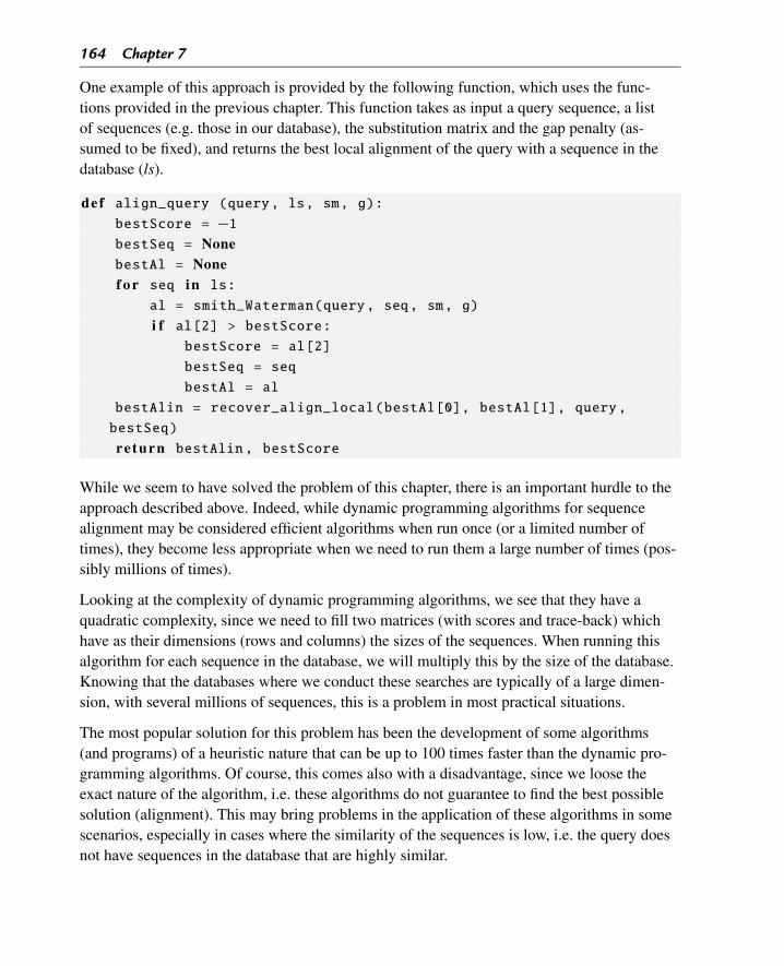
164 Chapter 7

One example of this approach is provided by the following function, which uses the func-tions provided in the previous chapter. This function takes as input a query sequence, a listof sequences (e.g. those in our database), the substitution matrix and the gap penalty (as-sumed to be fixed), and returns the best local alignment of the query with a sequence in thedatabase (ls).

def align_query (query, ls, sm, g):bestScore = −1bestSeq = NonebestAl = Nonef o r seq in ls:

al = smith_Waterman(query, seq, sm, g)

i f al[2] > bestScore:bestScore = al[2]

bestSeq = seq

bestAl = al

bestAlin = recover_align_local(bestAl[0], bestAl[1], query,

bestSeq)

re turn bestAlin, bestScore

While we seem to have solved the problem of this chapter, there is an important hurdle to theapproach described above. Indeed, while dynamic programming algorithms for sequencealignment may be considered efficient algorithms when run once (or a limited number oftimes), they become less appropriate when we need to run them a large number of times (pos-sibly millions of times).

Looking at the complexity of dynamic programming algorithms, we see that they have aquadratic complexity, since we need to fill two matrices (with scores and trace-back) whichhave as their dimensions (rows and columns) the sizes of the sequences. When running thisalgorithm for each sequence in the database, we will multiply this by the size of the database.Knowing that the databases where we conduct these searches are typically of a large dimen-sion, with several millions of sequences, this is a problem in most practical situations.

The most popular solution for this problem has been the development of some algorithms(and programs) of a heuristic nature that can be up to 100 times faster than the dynamic pro-gramming algorithms. Of course, this comes also with a disadvantage, since we loose theexact nature of the algorithm, i.e. these algorithms do not guarantee to find the best possiblesolution (alignment). This may bring problems in the application of these algorithms in somescenarios, especially in cases where the similarity of the sequences is low, i.e. the query doesnot have sequences in the database that are highly similar.

Searching Similar Sequences in Databases 165

A few heuristic algorithms have been proposed by the Bioinformatics community over thelast years, to address this task. The most popular ones are FASTA, that appeared in the earlydays of Bioinformatics, and BLAST (Basic Local Alignment Search Tool) that is now a widelyused program available to be run by the community in a large number of servers, including themain research institutes, as the NCBI or the EBI.

In the next section, we will use BLAST as an example and explore some of its algorithmicfeatures. The following section will contain a simplified Python version to exemplify the im-plementation of some of these features. The chapter closes with some examples of the use ofthe BLAST servers and programs using BioPython functions.

7.2 BLAST Algorithm and Programs

7.2.1 Overview of the BLAST Algorithm

The BLAST algorithm is currently the most used to perform searches over DNA or proteinsequence databases. The aim is to search for good alignments between a query sequence andthe sequences of a defined database. The basic idea of the algorithms is to use short “words”(i.e. sub-sequences) and search for matches of high similarity (with no gaps) of these words inthe query and in the sequences from the database. These matches will form a basis that can befurther extended, in both directions, to obtain high-quality alignments of larger dimension.

The main steps of the BLAST algorithm may be summarized in the following:

1. Remove regions of low complexity (e.g. sequence repeats) from the sequence that maycompromise the quality of the alignment;

2. Obtain all possible “words” of size w (a parameter of the algorithm), i.e. sub-sequencesof length w occurring in the query sequence;

3. For each word from the previous step, compile the list of all possible words of size w thatcan be defined in the allowable alphabet, whose alignment score (with no gaps) is higherthan a threshold T (parameter of the algorithm);

4. Search in all sequences from the database, all occurrences of the words collected in thelast step, which represent matches (hits) of size w between the query and one of thedatabase sequences;

5. Extend all hits from the last step, in both directions, while the score follows a given crite-rion (typically, the criterion is dependent on the size of the extension);

6. Select the alignments in the previous step with highest scores, normalized for its size(these are named the high-scoring pairs-HSPs).

In the most recent version of BLAST, from 1997, the criterion to extend alignments is moredemanding, requiring two near hits with scores above T separated by a distance smaller than

166 Chapter 7

a given parameter. This change leads to less extensions and a more efficient algorithm, whilethe obtained results are shown to be in a similar level. With this strategy, it is also possible toinclude gaps within the two hits, and as a result BLAST can return gapped alignments.

Notice that the parameters w and T are quite important in the set of returned results and algo-rithm’s efficiency. Choosing a smaller value of w or T increases sensitivity, i.e. the number ofinteresting sequences found, but also increases the processing time.

7.2.2 BLAST Programs

The described algorithm gave rise to a number of programs specific for different sequencetypes, which can be locally installed or run over distinct servers available in the web. Themost important of these servers is maintained by NCBI and can be accessed in the URLhttps://www.ncbi.nlm.nih.gov/BLAST.

The main programs are BLASTN and BLASTP, for nucleotide and protein searches. BLASTNcan be used to search different nucleotide databases for similar sequences, being the defaultthe nr/nt, a non-redundant collection of nucleotide sequences, while many other alternativesexist, including to filter by a given species genome, to use the RefSeq database, to consideronly ribosomal RNA sequences (16S), etc.

BLASTN allows to optimize the search for highly similar sequences, allowing a faster searchfor longer sequences (using the megablast program). In BLASTN, there are a number of pa-rameters that can be set including the word size w whose default value is 11, and the onesdefining the scoring function, the match/mismatch scores (default 2 and −3) and the gappenalties for opening and extension (default values of −5 and −2).

On the other hand, BLASTP can be used to search for protein sequence databases, such as thenr, the non-redundant set of protein sequences, RefSeq, UniProt (curated sequences from theSwissProt database) or sequences from the PDB database. The set of adjustable parametersare similar to BLASTN, with different default values: w is set to 6, while the scoring functionuses a substitution matrix (BLOSUM62 by default), and gap penalties for opening and exten-sion (default values of −11 and −1). For protein alignments, there are alternative programswhich are not covered in this book, such as PSI-BLAST, PHI-BLAST and DELTA-BLAST.

Also, there are three other programs in the BLAST suite which may be used to search for se-quences of a different type:

• BLASTX – takes a DNA sequence as query, but searches over protein sequences, and thuscan be used to find potential protein products encoded by a nucleotide sequence; the DNAsequence is translated considering all 6 reading frames (relevant definitions and algo-rithms may be found in Chapter 4);

Searching Similar Sequences in Databases 167

• TBLASTN – takes a protein sequence as query, but searches over DNA sequencedatabases, thus trying to identify database sequences encoding proteins similar to theone in the query; sequences from the databases are translated considering the 6 readingframes, prior to the alignments;

• TBLASTX – takes a DNA sequence as input, searching over DNA sequence databases,but in both cases the sequences are translated considering the 6 reading frames and thematches are searched over protein sequences (this leads to 36 comparisons); this methodcan be used to identify nucleotide sequences similar to the query based on their codingpotential.

7.2.3 Significance of the Alignments

One important aspect to discuss relates with the statistical significance of the alignments ob-tained. Although a detailed discussion on this subject is outside the scope of this book, wewill briefly explain the underlying problems and present the main metrics returned by theseprograms to address this issue.

The scoring functions used by BLAST and dynamic programming, based on substitutionmatrices and gap penalties, are relative to the size of the sequences. So, they are useful tocompare different alignments for the same pair of sequences, but cannot be used to comparealignments of different sequences with distinct sizes. So, when comparing hits of a query withother sequences of distinct sizes, there is the need to compute normalized scores that can beused to compare alignments of different sizes. BLAST computes normalized scores usingmeasures from information theory, and as such the normalized scores are provided in bits.

However, even these scores normalized for sequence size are not enough to compare any typeof alignment, and thus can not provide an answer to the question: is the similarity found be-tween the query and the sequence, for a given alignment, statistically significant? Or, in otherwords, how probable is that this similarity occurs by pure chance? These are important ques-tions to be able to infer possible homology from sequence similarity.

The most popular metric to evaluate the significance of the alignment, provided as a result foreach HSP in BLAST, is the E value. This value indicates the number of expected alignmentswith a score at least as high as the one provided by the current HSP. Although we will not dis-cuss details, this value is calculated taking into account the score of the alignment, the size ofthe database, and length of the sequences included, as well as the parameters of the alignment.

The lower the value of E is, i.e. the closer it is to zero, the more significant the consideredmatch is. It is difficult to define a threshold for what is considered significant, being used val-ues from 10−5 up to 0.05 in different scenarios and by different authors.

168 Chapter 7

When checking if an alignment indicates homology or not, it is also important not to rely onlyon the E value, but look also at other results. Since BLAST returns local alignments, it is offoremost importance to look at the coverage of the alignment in the query (and also in thesequence found), i.e. looking at which parts of the overall sequences are included in the align-ment proposed. This will help in understanding if there might be a global homology or justsimilarity in parts of the sequences (e.g. protein domains or other local patterns).

7.3 Implementing Our Own BLAST

In this section, we will build our own version of a very simplified version of BLAST, whichwe will name MyBlast. Although much simpler than BLAST itself, it will allow to get an ideaof some of the algorithmic constructions used to build these tools.

The first step in our MyBlast program will be to create a database. We will assume here thesimplest hypothesis: the database will be a list of sequences (strings), and we will define be-low a function to load this database from a text file, where each sequence will be in a separateline.

def read_database (filename):f = open (filename)db = []

f o r line in f:

db.append(line.rstrip())

f.close()

re turn db

The next step will be to pre-process the query, creating a map that will identify all words ofsize w (a parameter) occurring in it, keeping for each word the positions where it occurs. Thistechnique is commonly named hashing and if, in a first look, it seems a waste of time, it isvery useful if one needs to repeatedly find occurrences of these words in the query. The datastructure used to keep these results will be a Python dictionary, since it allows a very efficientaccess of the values associated to its keys.

Thus, the next function creates a dictionary (map) from the query sequence following thisidea. The dictionary returned has the words in the query as keys, and lists of positions wherethese occur as values.

def build_map (query, w):res = {}

f o r i in range( l e n (query)−w+1):

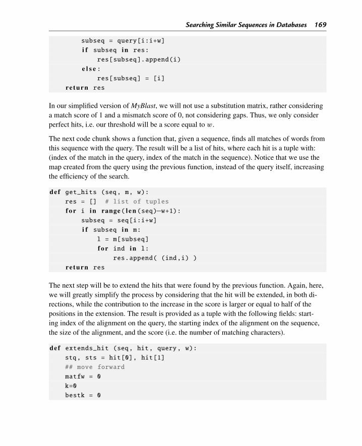
Searching Similar Sequences in Databases 169

subseq = query[i:i+w]

i f subseq in res:

res[subseq].append(i)

e l s e :res[subseq] = [i]

re turn res

In our simplified version of MyBlast, we will not use a substitution matrix, rather consideringa match score of 1 and a mismatch score of 0, not considering gaps. Thus, we only considerperfect hits, i.e. our threshold will be a score equal to w.

The next code chunk shows a function that, given a sequence, finds all matches of words fromthis sequence with the query. The result will be a list of hits, where each hit is a tuple with:(index of the match in the query, index of the match in the sequence). Notice that we use themap created from the query using the previous function, instead of the query itself, increasingthe efficiency of the search.

def get_hits (seq, m, w):res = [] # list of tuples

f o r i in range( l e n (seq)−w+1):subseq = seq[i:i+w]

i f subseq in m:

l = m[subseq]

f o r ind in l:

res.append( (ind,i) )

re turn res

The next step will be to extend the hits that were found by the previous function. Again, here,we will greatly simplify the process by considering that the hit will be extended, in both di-rections, while the contribution to the increase in the score is larger or equal to half of thepositions in the extension. The result is provided as a tuple with the following fields: start-ing index of the alignment on the query, the starting index of the alignment on the sequence,the size of the alignment, and the score (i.e. the number of matching characters).

def extends_hit (seq, hit, query, w):stq, sts = hit[0], hit[1]

## move forward

matfw = 0

k=0

bestk = 0

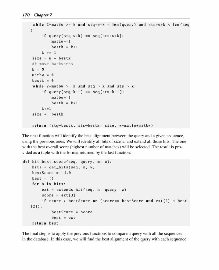
170 Chapter 7

whi le 2∗matfw >= k and stq+w+k < l e n (query) and sts+w+k < l e n (seq):

i f query[stq+w+k] == seq[sts+w+k]:matfw+=1

bestk = k+1

k += 1

size = w + bestk

## move backwards

k = 0

matbw = 0

bestk = 0

whi le 2∗matbw >= k and stq > k and sts > k:i f query[stq−k−1] == seq[sts−k−1]:

matbw+=1

bestk = k+1

k+=1

size += bestk

re turn (stq−bestk, sts−bestk, size, w+matfw+matbw)

The next function will identify the best alignment between the query and a given sequence,using the previous ones. We will identify all hits of size w and extend all those hits. The onewith the best overall score (highest number of matches) will be selected. The result is pro-vided as a tuple with the format returned by the last function.

def hit_best_score(seq, query, m, w):hits = get_hits(seq, m, w)

bestScore = −1.0best = ()

f o r h in hits:

ext = extends_hit(seq, h, query, w)

score = ext[3]

i f score > bestScore or (score== bestScore and ext[2] < best[2]):

bestScore = score

best = ext

re turn best

The final step is to apply the previous functions to compare a query with all the sequencesin the database. In this case, we will find the best alignment of the query with each sequence

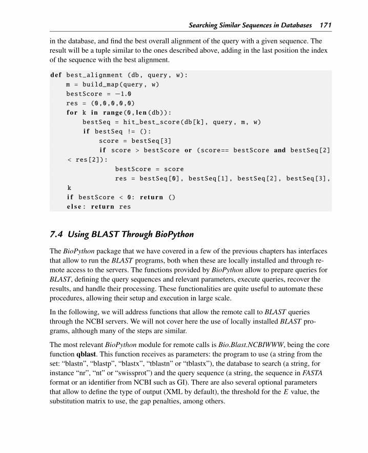
Searching Similar Sequences in Databases 171

in the database, and find the best overall alignment of the query with a given sequence. Theresult will be a tuple similar to the ones described above, adding in the last position the indexof the sequence with the best alignment.

def best_alignment (db, query, w):m = build_map(query, w)

bestScore = −1.0res = (0,0,0,0,0)

f o r k in range(0, l e n (db)):bestSeq = hit_best_score(db[k], query, m, w)

i f bestSeq != ():score = bestSeq[3]

i f score > bestScore or (score== bestScore and bestSeq[2]< res[2]):

bestScore = score

res = bestSeq[0], bestSeq[1], bestSeq[2], bestSeq[3],

k

i f bestScore < 0: re turn ()

e l s e : re turn res

7.4 Using BLAST Through BioPython

The BioPython package that we have covered in a few of the previous chapters has interfacesthat allow to run the BLAST programs, both when these are locally installed and through re-mote access to the servers. The functions provided by BioPython allow to prepare queries forBLAST, defining the query sequences and relevant parameters, execute queries, recover theresults, and handle their processing. These functionalities are quite useful to automate theseprocedures, allowing their setup and execution in large scale.

In the following, we will address functions that allow the remote call to BLAST queriesthrough the NCBI servers. We will not cover here the use of locally installed BLAST pro-grams, although many of the steps are similar.

The most relevant BioPython module for remote calls is Bio.Blast.NCBIWWW, being the corefunction qblast. This function receives as parameters: the program to use (a string from theset: “blastn”, “blastp”, “blastx”, “tblastn” or “tblastx”), the database to search (a string, forinstance “nr”, “nt” or “swissprot”) and the query sequence (a string, the sequence in FASTAformat or an identifier from NCBI such as GI). There are also several optional parametersthat allow to define the type of output (XML by default), the threshold for the E value, thesubstitution matrix to use, the gap penalties, among others.

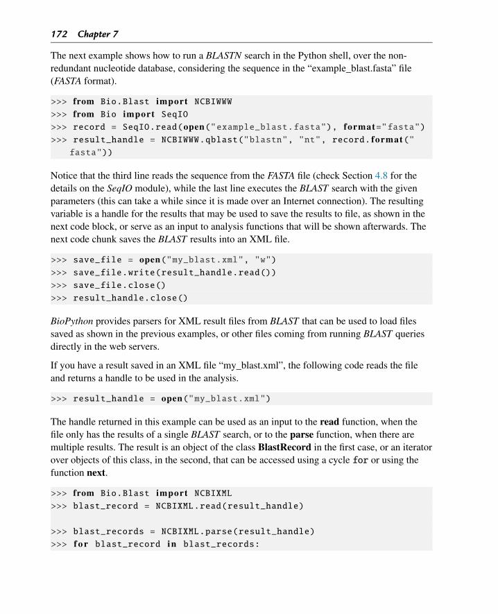
172 Chapter 7

The next example shows how to run a BLASTN search in the Python shell, over the non-redundant nucleotide database, considering the sequence in the “example_blast.fasta” file(FASTA format).

>>> from Bio.Blast import NCBIWWW>>> from Bio import SeqIO>>> record = SeqIO.read(open("example_blast.fasta"), format="fasta")>>> result_handle = NCBIWWW.qblast("blastn", "nt", record. format("fasta"))

Notice that the third line reads the sequence from the FASTA file (check Section 4.8 for thedetails on the SeqIO module), while the last line executes the BLAST search with the givenparameters (this can take a while since it is made over an Internet connection). The resultingvariable is a handle for the results that may be used to save the results to file, as shown in thenext code block, or serve as an input to analysis functions that will be shown afterwards. Thenext code chunk saves the BLAST results into an XML file.

>>> save_file = open("my_blast.xml", "w")>>> save_file.write(result_handle.read())

>>> save_file.close()

>>> result_handle.close()

BioPython provides parsers for XML result files from BLAST that can be used to load filessaved as shown in the previous examples, or other files coming from running BLAST queriesdirectly in the web servers.

If you have a result saved in an XML file “my_blast.xml”, the following code reads the fileand returns a handle to be used in the analysis.

>>> result_handle = open("my_blast.xml")

The handle returned in this example can be used as an input to the read function, when thefile only has the results of a single BLAST search, or to the parse function, when there aremultiple results. The result is an object of the class BlastRecord in the first case, or an iteratorover objects of this class, in the second, that can be accessed using a cycle for or using thefunction next.

>>> from Bio.Blast import NCBIXML>>> blast_record = NCBIXML.read(result_handle)

>>> blast_records = NCBIXML.parse(result_handle)

>>> f o r blast_record in blast_records:

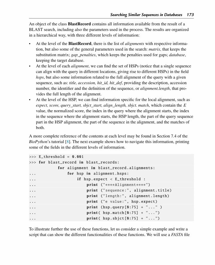
Searching Similar Sequences in Databases 173

An object of the class BlastRecord contains all information available from the result of aBLAST search, including also the parameters used in the process. The results are organizedin a hierarchical way, with three different levels of information:

• At the level of the BlastRecord, there is the list of alignments with respective informa-tion, but also some of the general parameters used in the search: matrix, that keeps thesubstitution matrix; gap_penalties, which keeps the penalties used for gaps; database,keeping the target database.

• At the level of each alignment, we can find the set of HSPs (notice that a single sequencecan align with the query in different locations, giving rise to different HSPs) in the fieldhsps, but also some information related to the full alignment of the query with a givensequence, such as: title, accession, hit_id, hit_def, providing the description, accessionnumber, the identifier and the definition of the sequence, or alignment.length, that pro-vides the full length of the alignment.

• At the level of the HSP, we can find information specific for the local alignment, such asexpect, score, query_start, sbjct_start, align_length, sbjct. match, which contain the E

value, the normalized score, the index in the query where the alignment starts, the indexin the sequence where the alignment starts, the HSP length, the part of the query sequencepart in the HSP alignment, the part of the sequence in the alignment, and the matches ofboth.

A more complete reference of the contents at each level may be found in Section 7.4 of theBioPython’s tutorial [8]. The next example shows how to navigate this information, printingsome of the fields in the different levels of information.

>>> E_threshold = 0.001

>>> f o r blast_record in blast_records:

f o r alignment in blast_record.alignments:

... f o r hsp in alignment.hsps:

... i f hsp.expect < E_threshold :

... p r i n t ("∗∗∗∗Alignment∗∗∗∗")

... p r i n t ("sequence:", alignment.title)

... p r i n t ("length:", alignment.length)

... p r i n t ("e value:", hsp.expect)

... p r i n t (hsp.query[0:75] + "..." )

... p r i n t ( hsp.match[0:75] + "...")

... p r i n t ( hsp.sbjct[0:75] + "...")

To illustrate further the use of these functions, let us consider a simple example and write ascript that can show the different functionalities of these functions. We will use a FASTA file

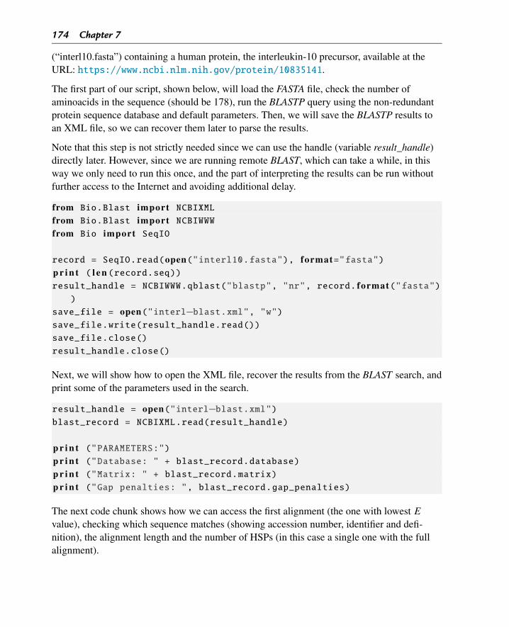
174 Chapter 7

(“interl10.fasta”) containing a human protein, the interleukin-10 precursor, available at theURL: https://www.ncbi.nlm.nih.gov/protein/10835141.

The first part of our script, shown below, will load the FASTA file, check the number ofaminoacids in the sequence (should be 178), run the BLASTP query using the non-redundantprotein sequence database and default parameters. Then, we will save the BLASTP results toan XML file, so we can recover them later to parse the results.

Note that this step is not strictly needed since we can use the handle (variable result_handle)directly later. However, since we are running remote BLAST, which can take a while, in thisway we only need to run this once, and the part of interpreting the results can be run withoutfurther access to the Internet and avoiding additional delay.

from Bio.Blast import NCBIXMLfrom Bio.Blast import NCBIWWWfrom Bio import SeqIO

record = SeqIO.read(open("interl10.fasta"), format="fasta")p r i n t ( l e n (record.seq))result_handle = NCBIWWW.qblast("blastp", "nr", record. format("fasta"))

save_file = open("interl−blast.xml", "w")save_file.write(result_handle.read())

save_file.close()

result_handle.close()

Next, we will show how to open the XML file, recover the results from the BLAST search, andprint some of the parameters used in the search.

result_handle = open("interl−blast.xml")blast_record = NCBIXML.read(result_handle)

p r i n t ("PARAMETERS:")p r i n t ("Database: " + blast_record.database)p r i n t ("Matrix: " + blast_record.matrix)p r i n t ("Gap penalties: ", blast_record.gap_penalties)

The next code chunk shows how we can access the first alignment (the one with lowest E

value), checking which sequence matches (showing accession number, identifier and defi-nition), the alignment length and the number of HSPs (in this case a single one with the fullalignment).

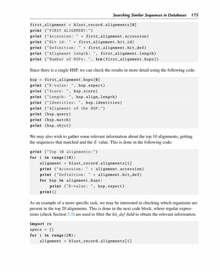
Searching Similar Sequences in Databases 175

first_alignment = blast_record.alignments[0]

p r i n t ("FIRST ALIGNMENT:")p r i n t ("Accession: " + first_alignment.accession)p r i n t ("Hit id: " + first_alignment.hit_id)p r i n t ("Definition: " + first_alignment.hit_def)p r i n t ("Alignment length: ", first_alignment.length)p r i n t ("Number of HSPs: ", l e n (first_alignment.hsps))

Since there is a single HSP, we can check the results in more detail using the following code:

hsp = first_alignment.hsps[0]

p r i n t ("E−value: ", hsp.expect)p r i n t ("Score: ", hsp.score)p r i n t ("Length: ", hsp.align_length)p r i n t ("Identities: ", hsp.identities)p r i n t ("Alignment of the HSP:")p r i n t (hsp.query)p r i n t (hsp.match)p r i n t (hsp.sbjct)

We may also wish to gather some relevant information about the top 10 alignments, gettingthe sequences that matched and the E value. This is done in the following code:

p r i n t ("Top 10 alignments:")f o r i in range(10):

alignment = blast_record.alignments[i]

p r i n t ("Accession: " + alignment.accession)p r i n t ("Definition: " + alignment.hit_def)f o r hsp in alignment.hsps:

p r i n t ("E−value: ", hsp.expect)p r i n t ()

As an example of a more specific task, we may be interested in checking which organisms arepresent in the top 20 alignments. This is done in the next code block, where regular expres-sions (check Section 5.5) are used to filter the hit_def field to obtain the relevant information.

import respecs = []

f o r i in range(20):alignment = blast_record.alignments[i]

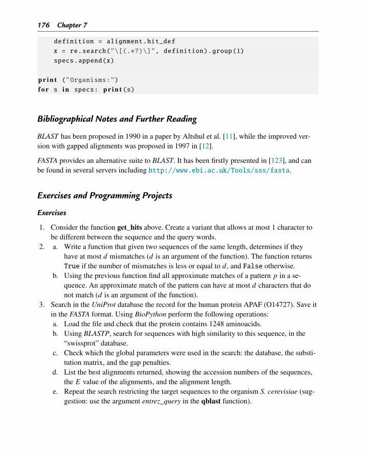
176 Chapter 7

definition = alignment.hit_def

x = re.search("\[(.∗?)\]", definition).group(1)specs.append(x)

p r i n t ("Organisms:")f o r s in specs: p r i n t (s)

Bibliographical Notes and Further Reading

BLAST has been proposed in 1990 in a paper by Altshul et al. [11], while the improved ver-sion with gapped alignments was proposed in 1997 in [12].

FASTA provides an alternative suite to BLAST. It has been firstly presented in [123], and canbe found in several servers including http://www.ebi.ac.uk/Tools/sss/fasta.

Exercises and Programming Projects

Exercises

1. Consider the function get_hits above. Create a variant that allows at most 1 character tobe different between the sequence and the query words.

2. a. Write a function that given two sequences of the same length, determines if theyhave at most d mismatches (d is an argument of the function). The function returnsTrue if the number of mismatches is less or equal to d , and False otherwise.

b. Using the previous function find all approximate matches of a pattern p in a se-quence. An approximate match of the pattern can have at most d characters that donot match (d is an argument of the function).

3. Search in the UniProt database the record for the human protein APAF (O14727). Save itin the FASTA format. Using BioPython perform the following operations:a. Load the file and check that the protein contains 1248 aminoacids.b. Using BLASTP, search for sequences with high similarity to this sequence, in the

“swissprot” database.c. Check which the global parameters were used in the search: the database, the substi-

tution matrix, and the gap penalties.d. List the best alignments returned, showing the accession numbers of the sequences,

the E value of the alignments, and the alignment length.e. Repeat the search restricting the target sequences to the organism S. cerevisiae (sug-

gestion: use the argument entrez_query in the qblast function).

Searching Similar Sequences in Databases 177

f. Check the results from the last operation, listing the best alignments, and checkingcarefully in each the start position of the alignment in the query and in the sequence.

g. What do you conclude about the existence of homologous genes in the yeast for thehuman protein APAF ?

Programming Projects

1. Improve the implementation of MyBlast by changing it to a class, which allows furtherconfiguration and considering the following variants:• Allow the database to be provided by an FASTA file, keeping in a dictionary the se-

quences and their descriptions.• Consider extending only those hits that have other hits in a neighborhood of less

than n positions (n should be a parameter of the function). In the extensions, you canuse dynamic programming to achieve the best alignment of the characters betweenthe hits.

• Add the option to use substitution matrices in the calculation of the matches. In thiscase, you should pre-compute all possible words of size w that score over T (T is aparameter) against words in the query, after mapping it. Adjust the hit extension forthis scenario, creating criteria for stopping extensions based on scores and extensionlength.

• Adapt the functions to allow returning a ranking of the best alignments, and not onlythe one that scores highest.

CHAPTER 8

Multiple Sequence Alignment

In this chapter, we generalize the alignment problem to consider multiple sequences and dis-cuss the impacts on the problem complexity and available algorithms. We review the mainclasses of optimization algorithms for this problem and discuss their main advantages andlimitations. Then, we focus on progressive alignment and implement a simplified version ofone of these algorithms in Python. We close the chapter reviewing how to handle alignmentsin BioPython.

8.1 Introduction: Problem Definition and Complexity

In Chapter 6, we have defined pairwise sequence alignment and discussed its need whenchecking for similarity between two biological sequences. We have looked at the problemcomplexity and have been able to find efficient algorithms to address its solution.

However, in many situations, we are faced with the need to align more than two sequences.This is of particular relevance, for instance, when determining the function of proteins, wherethe combination of different sequences with potential homology with our target, from distinctorganisms, can bring additional confidence in generating hypotheses for functional annota-tion, and provides a more reliable way to identify conserved regions of those proteins thatmight have a relevant functional role. Protein alignments can also greatly help in determiningtheir secondary or tertiary structures.

Also, in epidemiology, aligning DNA sequences of related organisms or strains is of foremostimportance to understand their evolution and regions of relevance for virulence factors. It isalso important to mention that there is a close relationship between multiple sequence align-ment and phylogenetic analysis which will be covered in the next chapter.

The problem of multiple sequence alignment (MSA) generalizes the pairwise alignment, con-sidering N (N > 2) sequences to be aligned. The aim of the alignment is the same as before:to introduce gaps in the sequences as a way to highlight the similar characters among them,placing similar characters in the same columns.

Note that MSAs can be global or local, as it happens with their pairwise counterparts. We willhere deal predominantly with glocal MSA, as the concept of local MSA is strongly related tomotif discovery, a topic that will be addressed in Chapters 10 and 11.

Bioinformatics Algorithms. DOI: 10.1016/B978-0-12-812520-5.00008-0Copyright © 2018 Elsevier Inc. All rights reserved. 179

180 Chapter 8

Although the definition of the problem is very similar, the complexity increases when thenumber of sequences grows. Indeed, the problem is considered NP-hard in terms of complex-ity. Thus, there are no efficient algorithms to solve the problem, when N becomes large.

One of the changes when handling MSA is the definition of the objective function in the for-mulation of the optimization problem. The objective function we used for pairwise sequencealignment was of an additive nature, summing the scores of the different columns to reach thefinal score. We will use the same strategy when scoring MSAs.

Also, the score of a column in pairwise alignment depends on the substitution matrix and thegap penalties defined. In MSA, these two components need also to be considered. Still, wealso need to deal with the fact that, in MSA, each column contains more than two characters.We, thus, need to define how to combine the multiple characters of a column and calculate ascore.

One common approach to address this is the sum of pairs (SP) method. In this case, for eachcolumn, we consider all possible pairs of the characters in this column and sum the respectivescores. We may choose to adapt the gap penalties to avoid over-penalizing columns with alarge number of gaps.

Let us provide an example. Consider the following alignment:

-RADNS

ARCD-A

AR-D-A

Using the BLOSUM62 matrix (check Fig. 6.3) and a penalty of g = −8 for each gap, the scoreSP of this alignment is the following:

Score = (sm(A,A) + g) + 3 × sm(R,R) + (sm(A,C) − g) + 3 × sm(D,D)

+(2 × g) + (2 × sm(S,A) + sm(A,A))

= (4 − 8) + 3 × 5 + (0 − 8) + 3 × 6 + (−8 × 2) + (1 + 1 + 4)

= 11

8.2 Classes of Optimization Algorithms for Multiple Sequence Alignment

8.2.1 Dynamic Programming

For pairwise alignment, we have already seen that there are efficient algorithms, based on Dy-namic Programming (DP), to solve those optimization problems, assuring optimal solutions,

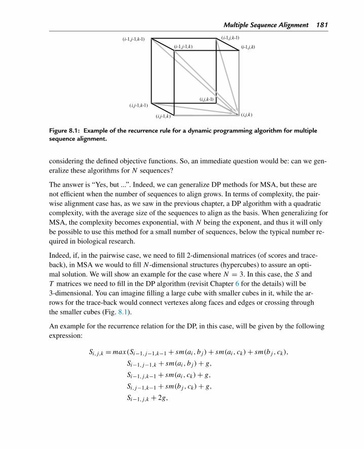
Multiple Sequence Alignment 181

Figure 8.1: Example of the recurrence rule for a dynamic programming algorithm for multiplesequence alignment.

considering the defined objective functions. So, an immediate question would be: can we gen-eralize these algorithms for N sequences?

The answer is “Yes, but ...”. Indeed, we can generalize DP methods for MSA, but these arenot efficient when the number of sequences to align grows. In terms of complexity, the pair-wise alignment case has, as we saw in the previous chapter, a DP algorithm with a quadraticcomplexity, with the average size of the sequences to align as the basis. When generalizing forMSA, the complexity becomes exponential, with N being the exponent, and thus it will onlybe possible to use this method for a small number of sequences, below the typical number re-quired in biological research.

Indeed, if, in the pairwise case, we need to fill 2-dimensional matrices (of scores and trace-back), in MSA we would to fill N -dimensional structures (hypercubes) to assure an opti-mal solution. We will show an example for the case where N = 3. In this case, the S andT matrices we need to fill in the DP algorithm (revisit Chapter 6 for the details) will be3-dimensional. You can imagine filling a large cube with smaller cubes in it, while the ar-rows for the trace-back would connect vertexes along faces and edges or crossing throughthe smaller cubes (Fig. 8.1).

An example for the recurrence relation for the DP, in this case, will be given by the followingexpression:

Si,j,k = max(Si−1,j−1,k−1 + sm(ai, bj ) + sm(ai, ck) + sm(bj , ck),

Si−1,j−1,k + sm(ai, bj ) + g,

Si−1,j,k−1 + sm(ai, ck) + g,

Si,j−1,k−1 + sm(bj , ck) + g,

Si−1,j,k + 2g,

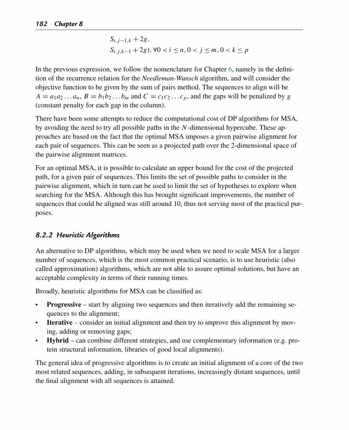
182 Chapter 8

Si,j−1,k + 2g,

Si,j,k−1 + 2g),∀0 < i ≤ n,0 < j ≤ m,0 < k ≤ p

In the previous expression, we follow the nomenclature for Chapter 6, namely in the defini-tion of the recurrence relation for the Needleman-Wunsch algorithm, and will consider theobjective function to be given by the sum of pairs method. The sequences to align will beA = a1a2 . . . an, B = b1b2 . . . bm and C = c1c2 . . . cp , and the gaps will be penalized by g

(constant penalty for each gap in the column).

There have been some attempts to reduce the computational cost of DP algorithms for MSA,by avoiding the need to try all possible paths in the N -dimensional hypercube. These ap-proaches are based on the fact that the optimal MSA imposes a given pairwise alignment foreach pair of sequences. This can be seen as a projected path over the 2-dimensional space ofthe pairwise alignment matrices.

For an optimal MSA, it is possible to calculate an upper bound for the cost of the projectedpath, for a given pair of sequences. This limits the set of possible paths to consider in thepairwise alignment, which in turn can be used to limit the set of hypotheses to explore whensearching for the MSA. Although this has brought significant improvements, the number ofsequences that could be aligned was still around 10, thus not serving most of the practical pur-poses.

8.2.2 Heuristic Algorithms

An alternative to DP algorithms, which may be used when we need to scale MSA for a largernumber of sequences, which is the most common practical scenario, is to use heuristic (alsocalled approximation) algorithms, which are not able to assure optimal solutions, but have anacceptable complexity in terms of their running times.

Broadly, heuristic algorithms for MSA can be classified as:

• Progressive – start by aligning two sequences and then iteratively add the remaining se-quences to the alignment;

• Iterative – consider an initial alignment and then try to improve this alignment by mov-ing, adding or removing gaps;

• Hybrid – can combine different strategies, and use complementary information (e.g. pro-tein structural information, libraries of good local alignments).

The general idea of progressive algorithms is to create an initial alignment of a core of the twomost related sequences, adding, in subsequent iterations, increasingly distant sequences, untilthe final alignment with all sequences is attained.

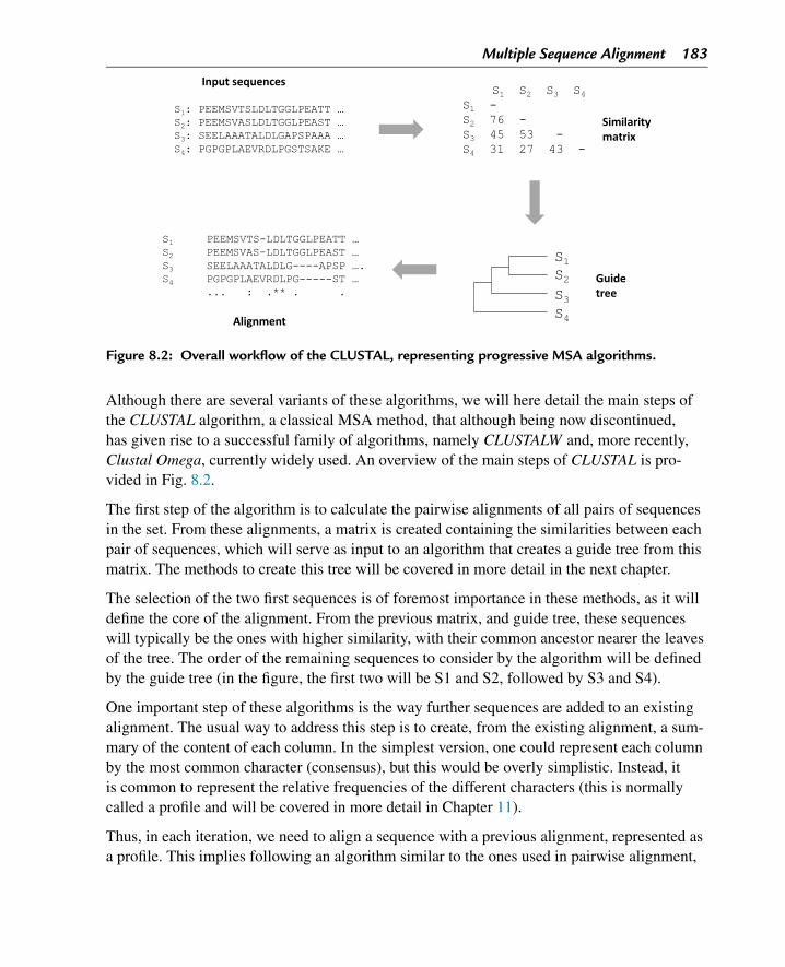
Multiple Sequence Alignment 183

Figure 8.2: Overall workflow of the CLUSTAL, representing progressive MSA algorithms.

Although there are several variants of these algorithms, we will here detail the main steps ofthe CLUSTAL algorithm, a classical MSA method, that although being now discontinued,has given rise to a successful family of algorithms, namely CLUSTALW and, more recently,Clustal Omega, currently widely used. An overview of the main steps of CLUSTAL is pro-vided in Fig. 8.2.

The first step of the algorithm is to calculate the pairwise alignments of all pairs of sequencesin the set. From these alignments, a matrix is created containing the similarities between eachpair of sequences, which will serve as input to an algorithm that creates a guide tree from thismatrix. The methods to create this tree will be covered in more detail in the next chapter.

The selection of the two first sequences is of foremost importance in these methods, as it willdefine the core of the alignment. From the previous matrix, and guide tree, these sequenceswill typically be the ones with higher similarity, with their common ancestor nearer the leavesof the tree. The order of the remaining sequences to consider by the algorithm will be definedby the guide tree (in the figure, the first two will be S1 and S2, followed by S3 and S4).

One important step of these algorithms is the way further sequences are added to an existingalignment. The usual way to address this step is to create, from the existing alignment, a sum-mary of the content of each column. In the simplest version, one could represent each columnby the most common character (consensus), but this would be overly simplistic. Instead, itis common to represent the relative frequencies of the different characters (this is normallycalled a profile and will be covered in more detail in Chapter 11).

Thus, in each iteration, we need to align a sequence with a previous alignment, represented asa profile. This implies following an algorithm similar to the ones used in pairwise alignment,

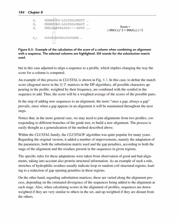
184 Chapter 8

Figure 8.3: Example of the calculation of the score of a column when combining an alignmentwith a sequence. The selected columns are highlighted. SM stands for the substitution matrixused.

but in this case adjusted to align a sequence to a profile, which implies changing the way thescore for a column is computed.

An example of this process in CLUSTAL is shown in Fig. 8.3. In this case, to define the matchscore (diagonal move in the S/T matrices in the DP algorithm), all possible characters ap-pearing in the profile, weighted by their frequency, are combined with the symbol in thesequence to add. Thus, the score will be a weighted average of the scores of the possible pairs.

In the step of adding new sequences to an alignment, the moto “once a gap, always a gap”prevails, since when a gap appears in an alignment it will be maintained throughout the nextsteps.

Notice that, in the more general case, we may need to join alignments from two profiles, cor-responding to different branches of the guide tree, to build a new alignment. The process iseasily thought as a generalization of the method described above.

Within the CLUSTAL family, the CLUSTALW algorithm was quite popular for many years.Regarding the original version, it added a number of improvements, namely the adaptation ofthe parameters, both the substitution matrix used and the gap penalties, according to both thestage of the alignment and the residues present in the sequences in given regions.

The specific rules for these adaptations were taken from observation of good and bad align-ments, taking into account also protein structural information. As an example of such a rule,stretches of hydrophilic residues usually indicate loop or random coil structural regions, lead-ing to a reduction of gap opening penalties in these regions.

On the other hand, regarding substitution matrices, these are varied along the alignment pro-cess, depending on the estimated divergence of the sequences being added to the alignment ateach stage. Also, when calculating scores in the alignment of profiles, sequences are down-weighted if they are very similar to others in the set, and up-weighted if they are distant fromthe others.

Multiple Sequence Alignment 185

Recently, the CLUSTAL family has switched to the use of the more recent CLUSTAL Omega.This algorithm greatly increased the efficiency of the algorithm used to create the guide treethat determines the order of the sequences in the alignments. Thus, it allows the algorithm tobe usable with a larger number of sequences (in the site at the EBI, they currently allow 4000,but report testing with over 100,000).

Although very popular and quite used in practice, progressive alignments have some prob-lems, mostly related to their heuristic greedy nature. Indeed, wrong decisions made in earlysteps of the alignment will not be corrected afterwards. The worst results of these algorithmsoccur when most of the sequences to align have low similarity.

An approach developed to counteract such problems has led to consistency based methods,from which the most well known is probably T-coffee. The idea is to maximize the agreementof pairwise alignments and, thus, try to avoid errors in the progressive algorithms. T-coffeebuilds libraries of global and local pairwise alignments, which are used to calculate weightsfor each position pair in each pairwise alignment. These weights are then used in the progres-sive alignment as scores in the DP algorithm when adding new sequences to the alignment.This method provides MSA solutions that are typically more accurate, but it suffers fromsome computational efficiency problems, not being suited for a large number of sequences,when compared for instance with ClustalOmega.

Iterative algorithms can be an alternative. They start by generating an alignment using a givenmethod, which may be a progressive alignment or any other method. Then, they try to im-prove this alignment by making selected changes and evaluating the effect of those changesover the objective function.

One alternative to improve the alignments is to repeatedly realign sub-groups of sequences,or sub-groups of columns, by changing the position of gaps or adding/removing gaps. Moreevolved optimization meta-heuristics, such as genetic algorithms, have also been tried, withsome success.

Hybrid algorithms include recent proposals such as MUSCLE, which combine progressivealignments based on profiles, with techniques from iterative methods, in this case workingby refining the guide tree to improve the resulting alignment. It is one of the more efficientmethods currently available.

On the other hand, the MAFFT algorithm brings the application of Fast Fourier Transforms(FFT) to MSA algorithms, being the sequences of aminoacid symbols converted into se-quences of volumes and polarities. FFTs allow to rapidly identify homologous regions, allow-ing fast algorithms for MSA, which also combine progressive and iterative methods. Recentversions allow a lot of flexibility in the configuration with different trade-offs of quality andspeed.

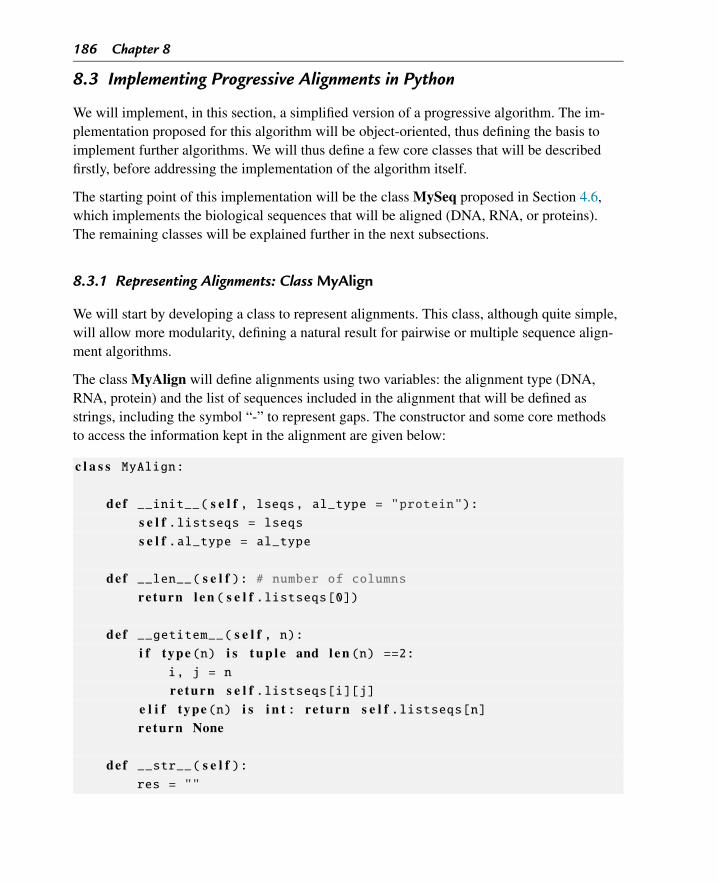
186 Chapter 8

8.3 Implementing Progressive Alignments in Python

We will implement, in this section, a simplified version of a progressive algorithm. The im-plementation proposed for this algorithm will be object-oriented, thus defining the basis toimplement further algorithms. We will thus define a few core classes that will be describedfirstly, before addressing the implementation of the algorithm itself.

The starting point of this implementation will be the class MySeq proposed in Section 4.6,which implements the biological sequences that will be aligned (DNA, RNA, or proteins).The remaining classes will be explained further in the next subsections.

8.3.1 Representing Alignments: Class MyAlign

We will start by developing a class to represent alignments. This class, although quite simple,will allow more modularity, defining a natural result for pairwise or multiple sequence align-ment algorithms.

The class MyAlign will define alignments using two variables: the alignment type (DNA,RNA, protein) and the list of sequences included in the alignment that will be defined asstrings, including the symbol “-” to represent gaps. The constructor and some core methodsto access the information kept in the alignment are given below:

c l a s s MyAlign:

def __init__( s e l f , lseqs, al_type = "protein"):s e l f .listseqs = lseqss e l f .al_type = al_type

def __len__( s e l f ): # number of columnsre turn l e n ( s e l f .listseqs[0])

def __getitem__( s e l f , n):i f type(n) i s t u p l e and l e n (n) ==2:

i, j = n

re turn s e l f .listseqs[i][j]e l i f type(n) i s i n t : re turn s e l f .listseqs[n]re turn None

def __str__( s e l f ):res = ""

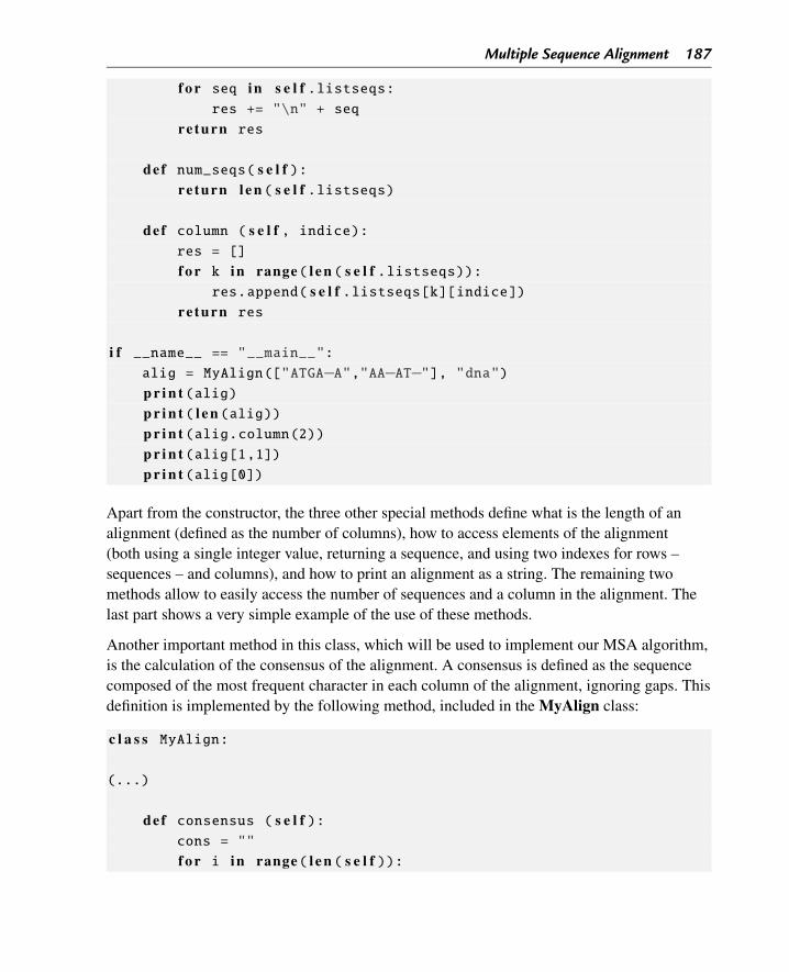
Multiple Sequence Alignment 187

f o r seq in s e l f .listseqs:res += "\n" + seq

re turn res

def num_seqs( s e l f ):re turn l e n ( s e l f .listseqs)

def column ( s e l f , indice):res = []

f o r k in range( l e n ( s e l f .listseqs)):res.append( s e l f .listseqs[k][indice])

re turn res

i f __name__ == "__main__":alig = MyAlign(["ATGA−A","AA−AT−"], "dna")p r i n t (alig)p r i n t ( l e n (alig))p r i n t (alig.column(2))p r i n t (alig[1,1])p r i n t (alig[0])

Apart from the constructor, the three other special methods define what is the length of analignment (defined as the number of columns), how to access elements of the alignment(both using a single integer value, returning a sequence, and using two indexes for rows –sequences – and columns), and how to print an alignment as a string. The remaining twomethods allow to easily access the number of sequences and a column in the alignment. Thelast part shows a very simple example of the use of these methods.

Another important method in this class, which will be used to implement our MSA algorithm,is the calculation of the consensus of the alignment. A consensus is defined as the sequencecomposed of the most frequent character in each column of the alignment, ignoring gaps. Thisdefinition is implemented by the following method, included in the MyAlign class:

c l a s s MyAlign:

(...)

def consensus ( s e l f ):cons = ""

f o r i in range( l e n ( s e l f )):

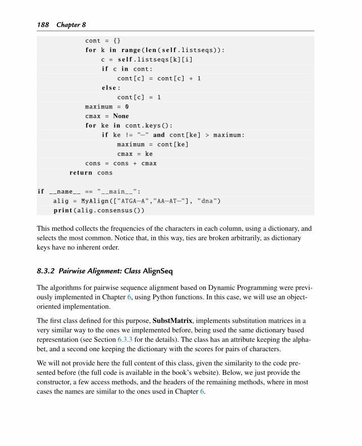
188 Chapter 8

cont = {}

f o r k in range( l e n ( s e l f .listseqs)):c = s e l f .listseqs[k][i]i f c in cont:

cont[c] = cont[c] + 1

e l s e :cont[c] = 1

maximum = 0

cmax = Nonef o r ke in cont.keys():

i f ke != "−" and cont[ke] > maximum:maximum = cont[ke]

cmax = ke

cons = cons + cmax

re turn cons

i f __name__ == "__main__":alig = MyAlign(["ATGA−A","AA−AT−"], "dna")p r i n t (alig.consensus())

This method collects the frequencies of the characters in each column, using a dictionary, andselects the most common. Notice that, in this way, ties are broken arbitrarily, as dictionarykeys have no inherent order.

8.3.2 Pairwise Alignment: Class AlignSeq

The algorithms for pairwise sequence alignment based on Dynamic Programming were previ-ously implemented in Chapter 6, using Python functions. In this case, we will use an object-oriented implementation.

The first class defined for this purpose, SubstMatrix, implements substitution matrices in avery similar way to the ones we implemented before, being used the same dictionary basedrepresentation (see Section 6.3.3 for the details). The class has an attribute keeping the alpha-bet, and a second one keeping the dictionary with the scores for pairs of characters.

We will not provide here the full content of this class, given the similarity to the code pre-sented before (the full code is available in the book’s website). Below, we just provide theconstructor, a few access methods, and the headers of the remaining methods, where in mostcases the names are similar to the ones used in Chapter 6.

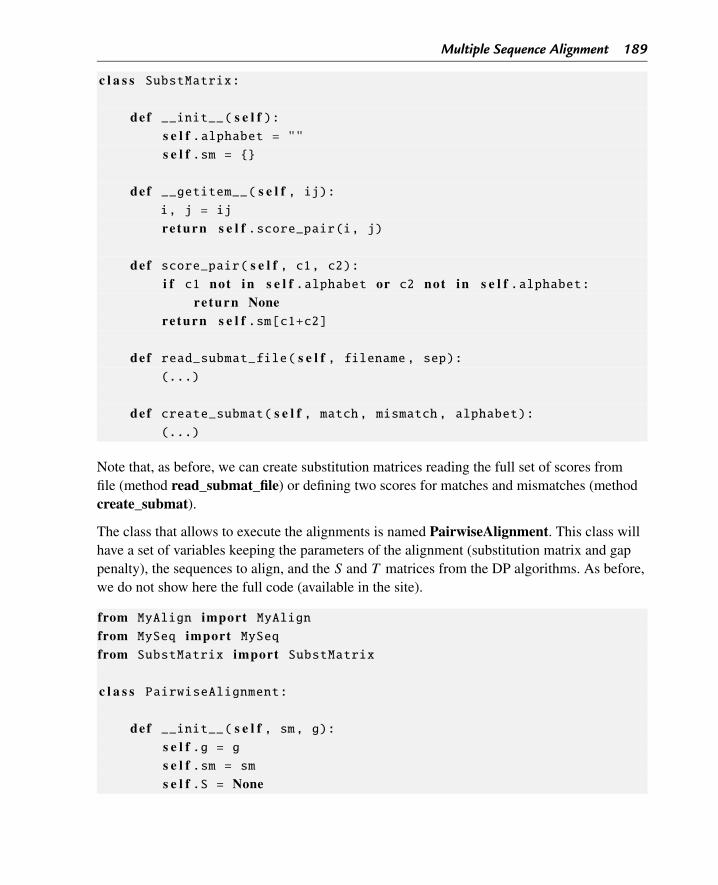
Multiple Sequence Alignment 189

c l a s s SubstMatrix:

def __init__( s e l f ):s e l f .alphabet = ""s e l f .sm = {}

def __getitem__( s e l f , ij):i, j = ij

re turn s e l f .score_pair(i, j)

def score_pair( s e l f , c1, c2):i f c1 not in s e l f .alphabet or c2 not in s e l f .alphabet:

re turn Nonereturn s e l f .sm[c1+c2]

def read_submat_file( s e l f , filename, sep):(...)

def create_submat( s e l f , match, mismatch, alphabet):(...)

Note that, as before, we can create substitution matrices reading the full set of scores fromfile (method read_submat_file) or defining two scores for matches and mismatches (methodcreate_submat).

The class that allows to execute the alignments is named PairwiseAlignment. This class willhave a set of variables keeping the parameters of the alignment (substitution matrix and gappenalty), the sequences to align, and the S and T matrices from the DP algorithms. As before,we do not show here the full code (available in the site).

from MyAlign import MyAlignfrom MySeq import MySeqfrom SubstMatrix import SubstMatrix

c l a s s PairwiseAlignment:

def __init__( s e l f , sm, g):s e l f .g = gs e l f .sm = sms e l f .S = None

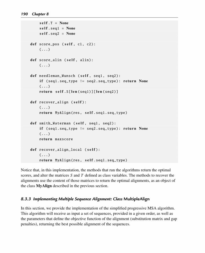
190 Chapter 8

s e l f .T = Nones e l f .seq1 = Nones e l f .seq2 = None

def score_pos ( s e l f , c1, c2):(...)

def score_alin ( s e l f , alin):(...)

def needleman_Wunsch ( s e l f , seq1, seq2):i f (seq1.seq_type != seq2.seq_type): re turn None(...)

re turn s e l f .S[ l e n (seq1)][ l e n (seq2)]

def recover_align ( s e l f ):(...)

re turn MyAlign(res, s e l f .seq1.seq_type)

def smith_Waterman ( s e l f , seq1, seq2):i f (seq1.seq_type != seq2.seq_type): re turn None(...)

re turn maxscore

def recover_align_local ( s e l f ):(...)

re turn MyAlign(res, s e l f .seq1.seq_type)

Notice that, in this implementation, the methods that run the algorithms return the optimalscores, and alter the matrices S and T defined as class variables. The methods to recover thealignments use the content of those matrices to return the optimal alignments, as an object ofthe class MyAlign described in the previous section.

8.3.3 Implementing Multiple Sequence Alignment: Class MultipleAlign

In this section, we provide the implementation of the simplified progressive MSA algorithm.This algorithm will receive as input a set of sequences, provided in a given order, as well asthe parameters that define the objective function of the alignment (substitution matrix and gappenalties), returning the best possible alignment of the sequences.

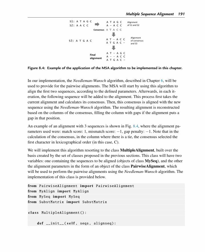
Multiple Sequence Alignment 191

Figure 8.4: Example of the application of the MSA algorithm to be implemented in this chapter.

In our implementation, the Needleman-Wunsch algorithm, described in Chapter 6, will beused to provide for the pairwise alignments. The MSA will start by using this algorithm toalign the first two sequences, according to the defined parameters. Afterwards, in each it-eration, the following sequence will be added to the alignment. This process first takes thecurrent alignment and calculates its consensus. Then, this consensus is aligned with the newsequence using the Needleman-Wunsch algorithm. The resulting alignment is reconstructedbased on the columns of the consensus, filling the column with gaps if the alignment puts agap in that position.

An example of an alignment with 3 sequences is shown in Fig. 8.4, where the alignment pa-rameters used were: match score: 1, mismatch score: −1, gap penalty: −1. Note that in thecalculation of the consensus, in the column where there is a tie, the consensus selected thefirst character in lexicographical order (in this case, C).

We will implement this algorithm resorting to the class MultipleAlignment, built over thebasis created by the set of classes proposed in the previous sections. This class will have twovariables: one containing the sequences to be aligned (objects of class MySeq), and the otherthe alignment parameters in the form of an object of the class PairwiseAlignment, whichwill be used to perform the pairwise alignments using the Needleman-Wunsch algorithm. Theimplementation of this class is provided below.

from PairwiseAlignment import PairwiseAlignmentfrom MyAlign import MyAlignfrom MySeq import MySeqfrom SubstMatrix import SubstMatrix

c l a s s MultipleAlignment():

def __init__( s e l f , seqs, alignseq):

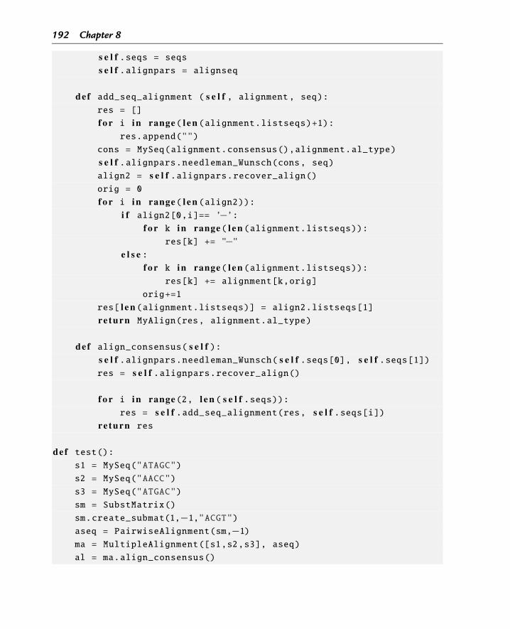
192 Chapter 8

s e l f .seqs = seqss e l f .alignpars = alignseq

def add_seq_alignment ( s e l f , alignment, seq):res = []

f o r i in range( l e n (alignment.listseqs)+1):res.append("")

cons = MySeq(alignment.consensus(),alignment.al_type)

s e l f .alignpars.needleman_Wunsch(cons, seq)align2 = s e l f .alignpars.recover_align()orig = 0

f o r i in range( l e n (align2)):i f align2[0,i]== ’−’:

f o r k in range( l e n (alignment.listseqs)):res[k] += "−"

e l s e :f o r k in range( l e n (alignment.listseqs)):

res[k] += alignment[k,orig]

orig+=1

res[ l e n (alignment.listseqs)] = align2.listseqs[1]re turn MyAlign(res, alignment.al_type)

def align_consensus( s e l f ):s e l f .alignpars.needleman_Wunsch( s e l f .seqs[0], s e l f .seqs[1])res = s e l f .alignpars.recover_align()

f o r i in range(2, l e n ( s e l f .seqs)):res = s e l f .add_seq_alignment(res, s e l f .seqs[i])

re turn res

def test():s1 = MySeq("ATAGC")

s2 = MySeq("AACC")

s3 = MySeq("ATGAC")

sm = SubstMatrix()

sm.create_submat(1,−1,"ACGT")aseq = PairwiseAlignment(sm,−1)ma = MultipleAlignment([s1,s2,s3], aseq)

al = ma.align_consensus()

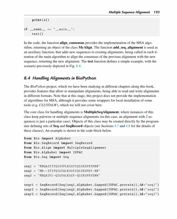
Multiple Sequence Alignment 193

p r i n t (al)

i f __name__ == "__main__":test()

In the code, the function align_consensus provides the implementation of the MSA algo-rithm, returning an object of the class MyAlign. The function add_seq_alignment is used asan auxiliary function, that adds new sequences to existing alignments, being called in each it-eration of the main algorithm to align the consensus of the previous alignment with the newsequence, returning the new alignment. The test function defines a simple example, with thescenario previously depicted in Fig. 8.4.

8.4 Handling Alignments in BioPython

The BioPython project, which we have been studying in different chapters along this book,provides features that allow to manipulate alignments, being able to read and write alignmentsin different formats. Note that at this stage, this project does not provide the implementationof algorithms for MSA, although it provides some wrappers for local installation of sometools (e.g. CLUSTALW), which we will not cover here.

The core class for handling alignments is MultipleSeqAlignment, where instances of thisclass keep pairwise or multiple sequence alignments (in this case, an alignment with 2 se-quences is just a particular case). Objects of this class may be created directly by the program-mer defining sets of Seq and SeqRecord objects (see Sections 4.7 and 4.8 for the details ofthese classes). An example is shown in the code block below.

from Bio import Alphabetfrom Bio.SeqRecord import SeqRecordfrom Bio.Align import MultipleSeqAlignmentfrom Bio.Alphabet import IUPACfrom Bio.Seq import Seq

seq1 = "MHQAIFIYQIGYPLKSGYIQSIRSPEYDNW"

seq2 = "MH−−IFIYQIGYALKSGYIQSIRSPEY−NW"seq3 = "MHQAIFI−QIGYALKSGY−QSIRSPEYDNW"

seqr1 = SeqRecord(Seq(seq1,Alphabet.Gapped(IUPAC.protein)), id ="seq1")seqr2 = SeqRecord(Seq(seq2,Alphabet.Gapped(IUPAC.protein)), id ="seq2")seqr3 = SeqRecord(Seq(seq3,Alphabet.Gapped(IUPAC.protein)), id ="seq3")

194 Chapter 8

alin = MultipleSeqAlignment([seqr1, seqr2, seqr3])

p r i n t (alin)

The alignments represented as objects of the class MultipleSeqAlignment, may be accessedthrough indexing in different ways. Using a single index, within squared brackets, we can in-dex rows (sequences), while two indexes, separated by a colon, will index rows and columns,respectively. In both indexes, we can use slicing to get intervals of sequences and/or columns.The following examples show some of the possibilities.

p r i n t (alin[1]) # 2nd sequencep r i n t (alin[:,2]) # 3rd columnp r i n t (alin[:,3:7]) # 4th to 7th columns (all sequences)

p r i n t (alin[0].seq[:3]) # first 3 columns of seq1p r i n t (alin[1:3,5:12]) # sequences 2 and 3; 4th to 10th column

Also, and similarly to what happens to sequences, BioPython also provides a class to allowinput/output operations of alignments in different formats, the class AlignIO. This includesthe methods read and parse, to read a single or multiple alignments, respectively, and themethod write that allows to write alignments to file. On the other hand, the method convertmay be used to directly convert between different alignment formats.

The following code reads a file with an alignment in the “clustal” format. The remaining ofthe code gets the number of columns in the alignment and prints its rows and identifiers of thesequences.

from Bio import AlignIOalin2 = AlignIO.read("PF05371_seed.aln", "clustal")

p r i n t ("Size:", alin2.get_alignment_length())f o r record in alin2:

p r i n t (record.seq, record. id )

Finally, in the next code block, we show two alternative ways of writing the previous align-ment to an FASTA file, by using the functions write and convert, respectively.

AlignIO.write(alin2, "example_alin.fasta", "fasta")

AlignIO.convert("PF05371_seed.aln", "clustal", "example_alin.fasta",

"fasta")

Multiple Sequence Alignment 195

Bibliographical Notes and Further Reading

Dynamic programming for multiple sequence alignment was proposed by Lipman et al. ina program named MSA [103], including some of the improvements that could increase effi-ciency, which were firstly proposed by Carrillo et al. in a previous paper [34].

Progressive alignments for MSA were firstly proposed by Feng and Doolitle in 1987 [63].The CLUSTAL algorithm was firstly proposed in 1988 [77], and improved in 1994 withCLUSTALW [147]. The most recent member of the family, Clustal Omega was proposed in2014 [139].

T-coffee was firstly published in 2000 [119]. On the other hand, the MUSCLE algorithm wasproposed in [58], while MAFFT has been firstly described in [87].

Exercises and Programming Projects

Exercises

1. Consider the following four sequences of DNA:

S1: ACATATCAT

S2: AACAGATCT

S3: AGATATTAG

S4: GCATCGATT

Write a Python script, using the code developed in this chapter, to generate a multiplealignment of these sequences using the progressive algorithm implemented in class Mul-tipleAlignment. Consider the parameters to be: match score = 1, mismatch = −1, gappenalty g = −1.

2. Implement a method calculating the score sum of pairs (SP) of a given alignment. Themethod should be included in the MultipleAlignment class, taking as input an alignment(object of class MyAlign). Notice that the parameters for the score are given in an inter-nal variable of the class (alignpars).

3. a. Consider the application of the Needleman-Wunsch algorithm to the protein se-quences: S1: APSC; S2: TAPT, using the BLOSUM62 matrix and g = −4. Calculatethe optimal alignment.

b. Based on the result of the previous exercise, could the following alignment be pro-vided by the progressive algorithm implemented in this chapter?

-AP-SC

TAPT--

TAT-S-

196 Chapter 8

c. Calculate the SP score of the previous alignment.d. Write a Python script, using the code developed in this chapter to confirm your re-

sults.4. Write a method to add to the class MyAlign that, given an alignment (self ), returns the

list of columns (indexes) in the alignment that are rich in polar basic aminoacids (R, H,or K). To be considered rich, the column needs to include at least half of the aminoacidsin this group.

5. Write a method to add to the class MyAlign that, given an alignment (self ), returns astring with a symbol for each column of the alignment, following these rules: ‘*’, if thecolumn is fully conserved (it has all symbols equal and no gaps); ‘:’, if the column has atleast half of the symbols equal; ‘.’: if the column does not match any of the previous, buthas no gaps; ‘ ’, in all other cases.

6. Write a method to add to the class MultipleAlign that, given an alignment (object ofclass MyAlign), identifies the columns where this alignment has high quality. In thiscase, a column is considered of high quality if the score of the alignment, calculated bythe SP method is larger than 0. The method should return a list of indexes of the selectedcolumns.

7. Consider the following sequence of aminoacids:

MEEPQSDPSVEPPLSQETFSDLWKLLPENNVLSPLPSQAMDDLMLSPDDIEQWFTE

DPGPDEAPRMPEAAPPVAPAPAAPTPAAPAPAPSWPLSSSVPSQKTYQGSYGFRLG

FLHSGTAKSVTCTYSPALNKMFCQLAKTCPVQLWVDSTPPPGTRVRAMAIYKQSQH

MTEVVRRCPHHERCSDSDGLAPPQHLIRVEGNLRVEYLDDRNTFRHSVVVPYEPPE

VGSDCTTIHYNYMCNSSCMGGMNRRPILTIITLEDSSGNLLGRNSFEVRVCACPGR

DRRTEEENLRKKGEPHHELPPGSTKRALPNNTSSSPQPKKKPLDGEYFTLQIRGRE

RFEMFRELNEALELKDAQAGKEPGGSRAHSSHLKSKKGQSTSRHKKLMFKTEGPDSD

a. Through the NCBI site, use the BLASTP application to search for similar sequences(alternatively use BioPython interface for this purpose) – see Chapter 7 for details.

b. From the result, select 10 to 12 matching sequences. Try to select different speciesand avoid sequences marked as “PREDICTED”. Save those into a file in the FASTAformat. Keep as sequence identifiers (after the “>” in the first line) the species name,without spaces.

c. In the EBI site, use the Clustal Omega application to get a multiple sequence align-ment using the previous set of sequences. Save the alignment (in the “clustal” for-mat) and the guide tree in two different files.

d. Load the previous alignment using BioPython.e. Calculate the consensus of the alignment. Suggestion: check the class AlignInfo in

the BioPython documentation or implement a function yourself.

Multiple Sequence Alignment 197

f. Calculate a list of positions where the alignment is conserved (i.e. all sequences havethe same aminoacid and there are no gaps). Calculate the percentage of these posi-tions in the whole alignment.

g. From the previous information, get the region of the alignment more conserved, i.e.the longest sequence of consecutive conserved positions from the list above.

Programming Projects

1. Complete the definition of the classes provided in this chapter (MySeq, MyAlign, Subst-Matrix, PairwiseAlignment, MultipleAlignment) with suitable methods coming fromthe concepts and algorithms from the previous chapters (including exercises), written inan object-oriented paradigm.

2. Add methods to the MultipleAlignment class that allow to consider the alignment ofprofiles with sequences. Redefine the MSA algorithm, allowing the user to input theguide tree of the alignment and use it to build the MSA.

3. Considering the class MultipleAlign developed above, implement an iterative algorithm.This should first create an alignment by randomly adding gaps to each sequence (thenumber of gaps per sequence may be defined by a user parameter). Implement methodsto allow adding and removing gaps from the alignment. Using these methods, implementan iterative algorithm that tries changes over the alignment, keeping the ones improvingthe alignment. Try to implement more intelligent changes over the alignments.

4. Implement a Dynamic Programming algorithm for MSA considering 3 sequences, ac-cording to what was defined above. Adapt the algorithm for different scoring models,namely in the gap penalties.

CHAPTER 9

Phylogenetic AnalysisIn this chapter, we review phylogenetic analysis problems and related algorithms, i.e. thoseaddressing the construction of phylogenetic trees from sequences. We discuss the main classesof algorithms to address the problem, focusing on distance-based approaches, and providinga Python implementation for one of the simplest algorithms. We also check some of the Bio-Python’s resources to handle phylogenetic trees.

9.1 Introduction: Problem Definition and Relevance

Phylogenetics is the branch of Biology which studies the evolutionary history and relation-ships among individuals or species. The inference of philogenies, represented as phylogenetictrees that explain the evolutionary relationship among these individuals or species, has tra-ditionally been achieved based on heritable traits, mainly morphological. The availability ofDNA sequences has allowed to reshape this field, making it much more rigorous, since it isbased on the direct product of evolution, given that mutations occur directly over DNA.

Thus, in the context of Bioinformatics, phylogenetic analysis is concerned with the determina-tion of how a given set of sequences has evolved from a common ancestor through a processof natural evolution. This evolutionary process is depicted in the form of an evolutionary tree,where bifurcations represent events of mutation from a common ancestor, that give rise to two(or more) different branches.

A phylogenetic tree will represent known sequences (DNA, RNA, protein) in its leaves (typ-ically from different species or other taxonomic categories), while internal tree nodes willrepresent common ancestors of the sequences below (see Fig. 9.1). Note that we will here dis-cuss mainly rooted trees, with a unique node, the root, that will correspond to the commonancestral of all sequences (taxa).

The structure of a rooted tree may be represented by the clusters (sets of sequences) coveredby each internal node. For instance, the tree in Fig. 9.1 may be represented by the sets: {1,2},{3,4}, {1,2,3,4}, {1,2,3,4,5}, not being here represented the trivial sets with the individualsequences. The height of the nodes in the tree represent a measure of time, and traveling fromthe root to the leaves represents the passage of time.

There are also unrooted trees, which are mainly used to illustrate the relationships among theleaves without explicitly representing or inferring the common ancestral. These will not be

Bioinformatics Algorithms. DOI: 10.1016/B978-0-12-812520-5.00009-2Copyright © 2018 Elsevier Inc. All rights reserved. 199

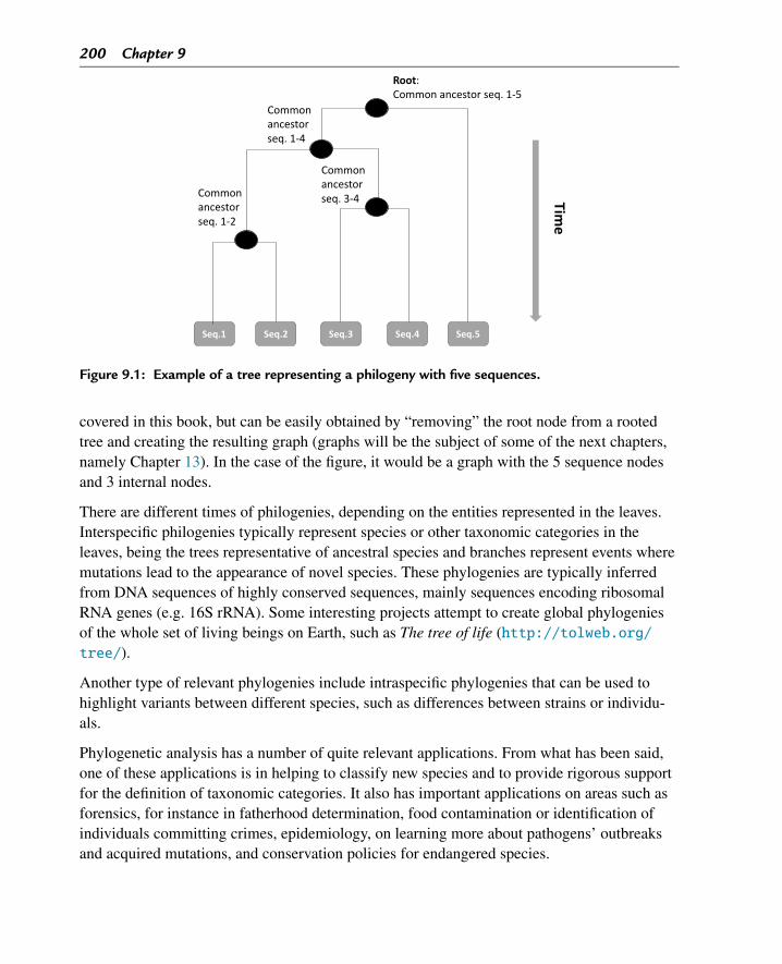
200 Chapter 9

Figure 9.1: Example of a tree representing a philogeny with five sequences.

covered in this book, but can be easily obtained by “removing” the root node from a rootedtree and creating the resulting graph (graphs will be the subject of some of the next chapters,namely Chapter 13). In the case of the figure, it would be a graph with the 5 sequence nodesand 3 internal nodes.

There are different times of philogenies, depending on the entities represented in the leaves.Interspecific philogenies typically represent species or other taxonomic categories in theleaves, being the trees representative of ancestral species and branches represent events wheremutations lead to the appearance of novel species. These phylogenies are typically inferredfrom DNA sequences of highly conserved sequences, mainly sequences encoding ribosomalRNA genes (e.g. 16S rRNA). Some interesting projects attempt to create global phylogeniesof the whole set of living beings on Earth, such as The tree of life (http://tolweb.org/tree/).

Another type of relevant phylogenies include intraspecific phylogenies that can be used tohighlight variants between different species, such as differences between strains or individu-als.

Phylogenetic analysis has a number of quite relevant applications. From what has been said,one of these applications is in helping to classify new species and to provide rigorous supportfor the definition of taxonomic categories. It also has important applications on areas such asforensics, for instance in fatherhood determination, food contamination or identification ofindividuals committing crimes, epidemiology, on learning more about pathogens’ outbreaksand acquired mutations, and conservation policies for endangered species.

Phylogenetic Analysis 201

On the level of functional annotation, phylogenies of protein sequences can be of importance,together with sequence alignment (as studied in the previous chapters), to better understandthe functions of specific sequences, and relate conserved domains to their functional roles.

The computational problem of inferring a phylogeny can be defined as the one of outputtingthe best possible evolutionary tree, given as the input the set of sequences assumed to be evo-lutionary related and, thus, deriving from a common ancestor. This is clearly an optimizationproblem, since for a given set of sequences there are a number of possible alternative treesthat could explain their evolution from a common ancestor.

The underlying optimization task is likely to be very complex since the number of possibletrees grows very rapidly, even for a moderate number of sequences in the input. For example,for a scenario of 30 sequences to create a tree, we would have around 1040 different trees,a number that clearly shows the complexity of the problem.

Before proceeding, and to define a proper optimization problem, we need to define suitableobjective functions that could be prone to mathematical optimization. This is a hard task thathas been addressed in different ways by the numerous distinct algorithms and tools that havebeen proposed for this problem. We will cover those in the next section, together with themain classes of available algorithms.

9.2 Classes of Algorithms for Phylogenetic Analysis

The algorithms for phylogenetic analysis can be broadly classified into three main classes,which mainly differ on the strategy used to compute the objective function, while also propos-ing alternative approaches to search over the huge solution space for this problem. The mainclasses are the following:

• Distance-based algorithms: includes methods based on the previous computation of amatrix of pairwise distances among the sequences (based on the sequence alignment),seeking to find the trees where the distances are consistent with the ones in the input ma-trix;

• Maximum parsimony: includes methods that search for the trees where the number ofneeded mutations (in internal nodes of the tree) to explain the variability of the sequencesis minimized;

• Statistical/Bayesian methods: defines probabilistic models for the occurrence of differ-ent types of mutations, and uses those models to score trees based on their probability (orlikelihood), searching for the most likely trees that explain the sequences according to theassumed model.

In this book, we will give an emphasis to the methods on the first group, while trying to pro-vide an overview over the remaining classes. This will be done in the next subsections.

202 Chapter 9

9.2.1 Distance-Based Methods

Distance-based methods for phylogeny inference rely on objective functions that measurethe consistency of the distances between the leaves (representing sequences) in the tree, withthe ones obtained from sequence similarity (through sequence alignment). Thus, the methodswill try to adjust the structure of the tree and the length of the edges connecting the nodes tomimic the pairwise distances between sequences.

The first step in distance-based methods is the definition of a matrix of distances betweenthe sequences. In this case, distance will be the reverse of similarity, and the methods used tocalculate these distances will consist on aligning the sequences and calculating the distancesbased on this alignment.

One simple way of achieving this task is to calculate the percentage of columns where thealignment contains mismatches or gaps. Of course, more sophisticated distance functions maybe defined using the set of parameters for pairwise alignment discussed in Chapter 6.

Given the matrix of distances, the objective function may be defined as an error function, thattries to minimize the differences between the distances in the tree and the distances in the ma-trix. One common approach is to consider the sum of squared errors:

score(T ) =∑i,j∈S

(dij (T ) − Dij )2 (9.1)

where S is the set of input sequences, T represents the tree (solution to be scored), dij (T )

represents the distance of the leaves representing sequences i and j in the tree T , and Dij

represents the distance between sequences i and j in the input matrix D given from sequencealignment.

Note that the distance between two nodes (u and v) in a rooted phylogenetic tree T is relatedto the vertical distances traveled from the origin u to the destination v. If w is the nearestcommon ancestor of u and v, the distance between u and v is given by the sum of duw + dwv .In the tree from Fig. 9.1, for instance, to travel between the leaves representing sequences 1and 4 would imply going from sequence 1 to the common ancestor of sequences 1 to 4, andtraveling back down to sequence 4. Both these distances are computed by the difference of theheights of the nodes: duw = h(w) − h(u) and dwv = h(w) − h(v), where h(x) denotes theheight of node x (note that d(w) is larger than d(u) and d(v), since w is a common ancestorof u and v).

If we assume the molecular clock hypothesis, that states that the mutation rate in all branchesof the tree is uniform, this implies the distance between all leaves and the root is the same (asit is the case with the tree in the figure). In this case, the tree is ultrametric and the height of

Phylogenetic Analysis 203

each leaf can be defined as 0. Therefore, in the previous expression, we would have duv =2 × h(w).

Given an objective function based on these general principles, a number of methods have beenproposed. Unfortunately, when the number of sequences grows, the solution space grows veryrapidly, and the problem has been proven to be NP-hard. As such, there are no algorithms thatcan efficiently provide guaranteed optimal solutions for reasonable dimensions (number ofsequences).

So, most algorithms used in practice are heuristic, providing reasonable solutions in prac-tice for most of the problem instances. One of the simplest and most popular methods inUnweighted Pair Group Method Using Arithmetic Averages (UPGMA), which is based onagglomerative hierarchical clustering algorithms.

This algorithm firstly considers each sequence (tree leaf) to be in its own cluster, whichare put at height zero in the tree. The algorithm starts by considering the pair of closest se-quences/clusters (i.e. the minimum value in the matrix D), and joining these sequencescreating an internal node, with height in the tree equal to half of the distance between thesesequences.

Those sequences will act, in the next iteration as a single cluster (merging the two clusterswith each sequence), being the distances to the remaining sequences/clusters calculated by theaverage of the distances, and leading to an update of D where the columns and rows of theconnected sequences disappear and a new row and new column appear for the new cluster.

In subsequent iterations, the algorithm proceeds by finding the pair of clusters with minimumdistances and repeating the same steps: joining the clusters, adding an internal node to thetree with the given height and updating the distance matrix D. The algorithm stops when allsequences are within a single cluster, which corresponds to the root node of the tree.

An example of the application of the UPGMA algorithm is shown in Fig. 9.2 to a set of fivesequences. The input distance matrix is shown in the upper left corner. In the first step, clus-ters representing sequences 1 and 2 are merged, being the respective internal node in the treeplaced at height h = 1. The matrix D is updated removing the rows and columns for se-quences 1 and 2, and creating new ones for the new cluster. The distances of this cluster tothe remaining are calculated by the mean of the distances of the sequences in the cluster (se-quences 1 and 2, in this case) to the remaining.

In the following step, clusters representing sequences 4 and 5 are merged, and the algorithmproceeds in a similar manner as for the previous ones. The third step merges the cluster ofsequences 1 and 2 with the one of sequence 3, while the final step merges the two remainingclusters.

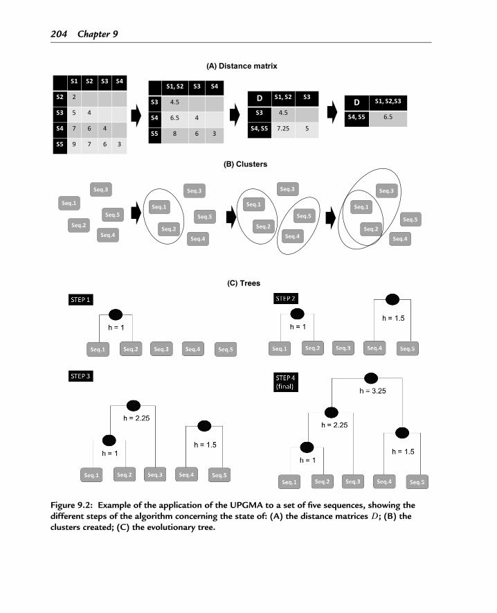
204 Chapter 9

Figure 9.2: Example of the application of the UPGMA to a set of five sequences, showing thedifferent steps of the algorithm concerning the state of: (A) the distance matrices D; (B) theclusters created; (C) the evolutionary tree.

Phylogenetic Analysis 205

As a general rule, in UPGMA, the distance between two clusters A and B is calculated aver-aging the distances of all pairs made from elements of both sets:

1

|A|.|B|∑i∈A

∑j∈B

Dij (9.2)

Within the execution of the algorithm, clusters are merged. If, in a given iteration, clusters A

and B are joined to obtain a new cluster (A ∪ B), the distances from the new cluster to eachcluster X can be calculated by a weighted average of the distances already calculated in thematrix:

D(A ∪ B,X) = |A|.D(A,X) + |B|.D(B,X)

|A| + |B| (9.3)

where D(X,Y ) here represents the distance of clusters X and Y in D.

An alternative is to use the algorithm WPGMA (Weighted Pair Group Method with ArithmeticMean) where the distances of new clusters to existing ones are calculated as the arithmeticmean of the distances of the joined clusters:

D(A ∪ B,X) = D(A,X) + D(B,X)

2(9.4)

The UPGMA algorithm is quite simple and has gained popularity in the community, but suf-fers from many limitations. One of the assumptions of the algorithm is that the mutation rateis uniform and, thus, the trees are ultrametric. If the input distance matrix is ultrametric, thealgorithm returns the optimal solution. However, this is an assumption that is rarely true inpractice and which leads to erroneous results in many situations.

An alternative method is Neighbor Joining (NJ), originally created to infer unrooted trees,and that does not assume the constant mutation rates across the different lineages. Note that,although it creates unrooted trees, the result of the NJ algorithm is in some cases given as arooted tree, by adding a root. There are different ways to do so, being the most used to placethe root at the midpoint of the longest distance connecting two leaves in the tree.

The main difference of NJ, when compared to UPGMA, is that the criterion to select the clus-ters to merge in each step does not only take into account the distances between the clusters,but also seeks to select cluster pairs where the nodes are apart from the other ones. To achievethis purpose, the original distance matrix D is pre-processed to create a new matrix Q, whereeach cell is calculated as:

Qij = (n − 2)Dij −n∑

k=1

Dik −n∑

k=1

Djk (9.5)

206 Chapter 9

It will be this matrix Q that will be used to select the nearest clusters in each step, as it is thecase in UPGMA. Notice that this implies that the clusters to be merged (or the nodes thatwill be joined by edges) are selected based on a trade-off, seeking pairs of nodes that have ashortest distance among themselves (first term of the previous expression) and that have largedistances from other clusters (measured by the last two sums in the previous expression).

In each step of the algorithm, the matrix D is recalculated. Taking u as the new cluster (newnode in the tree) created joining nodes a and b, the distances from the other clusters/nodes(represented as i) are calculated as:

Dui = 1

2(Dai + Dbi − Dab) (9.6)

From this new matrix D, the new matrix Q is recalculated applying the expression givenabove, and the algorithm proceeds by choosing the minimum value to select the clusters tomerge (nodes to join).

9.2.2 Maximum Parsimony

The maximum parsimony methods define the objective functions of the phylogenetic infer-ence problem by estimating the number of mutations that are implied by the tree to explainthe input sequences. Thus, in principle, shorter trees that explain the data are preferred, fol-lowing the Occam’s razor principle that states a preference for simpler models.

These methods are typically based on a previously defined multiple sequence alignment ofthe input sequences, which allows to identify a set of columns in the alignment that are con-sidered informative about the possible philogeny, namely columns where there are mutations(gaps or mismatches) and thus variations of the different sequences. From this information,this method tries to identify the tree that requires the minimum number of mutations to ex-plain the variations in the sequences.

The simplest way of identifying the most parsimonious tree is the enumeration of all possi-ble solutions and their cost. However, this is again an NP-hard problem, which implies thatthis is a non-viable strategy in practice, being only possible to achieve for a small number ofsequences (typically less than 10).

An alternative which has been proposed for this problem is the use of branch and boundmethods (we will cover those in more detail in the context of motif discovery in Chapter 10).In this case, an exact solution will still be found, but without having to test all possible trees,since some areas of the search space may be discarded since we have guaranteed that these donot contain the optimal solution. In practice, this allows to increase the number of sequencesin the input, still guaranteeing optimal solutions, up to about 20 sequences.

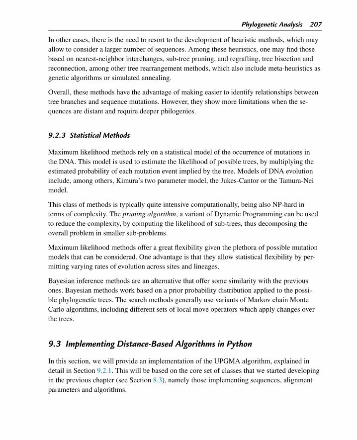
Phylogenetic Analysis 207

In other cases, there is the need to resort to the development of heuristic methods, which mayallow to consider a larger number of sequences. Among these heuristics, one may find thosebased on nearest-neighbor interchanges, sub-tree pruning, and regrafting, tree bisection andreconnection, among other tree rearrangement methods, which also include meta-heuristics asgenetic algorithms or simulated annealing.

Overall, these methods have the advantage of making easier to identify relationships betweentree branches and sequence mutations. However, they show more limitations when the se-quences are distant and require deeper philogenies.

9.2.3 Statistical Methods

Maximum likelihood methods rely on a statistical model of the occurrence of mutations inthe DNA. This model is used to estimate the likelihood of possible trees, by multiplying theestimated probability of each mutation event implied by the tree. Models of DNA evolutioninclude, among others, Kimura’s two parameter model, the Jukes-Cantor or the Tamura-Neimodel.

This class of methods is typically quite intensive computationally, being also NP-hard interms of complexity. The pruning algorithm, a variant of Dynamic Programming can be usedto reduce the complexity, by computing the likelihood of sub-trees, thus decomposing theoverall problem in smaller sub-problems.

Maximum likelihood methods offer a great flexibility given the plethora of possible mutationmodels that can be considered. One advantage is that they allow statistical flexibility by per-mitting varying rates of evolution across sites and lineages.

Bayesian inference methods are an alternative that offer some similarity with the previousones. Bayesian methods work based on a prior probability distribution applied to the possi-ble phylogenetic trees. The search methods generally use variants of Markov chain MonteCarlo algorithms, including different sets of local move operators which apply changes overthe trees.

9.3 Implementing Distance-Based Algorithms in Python

In this section, we will provide an implementation of the UPGMA algorithm, explained indetail in Section 9.2.1. This will be based on the core set of classes that we started developingin the previous chapter (see Section 8.3), namely those implementing sequences, alignmentparameters and algorithms.

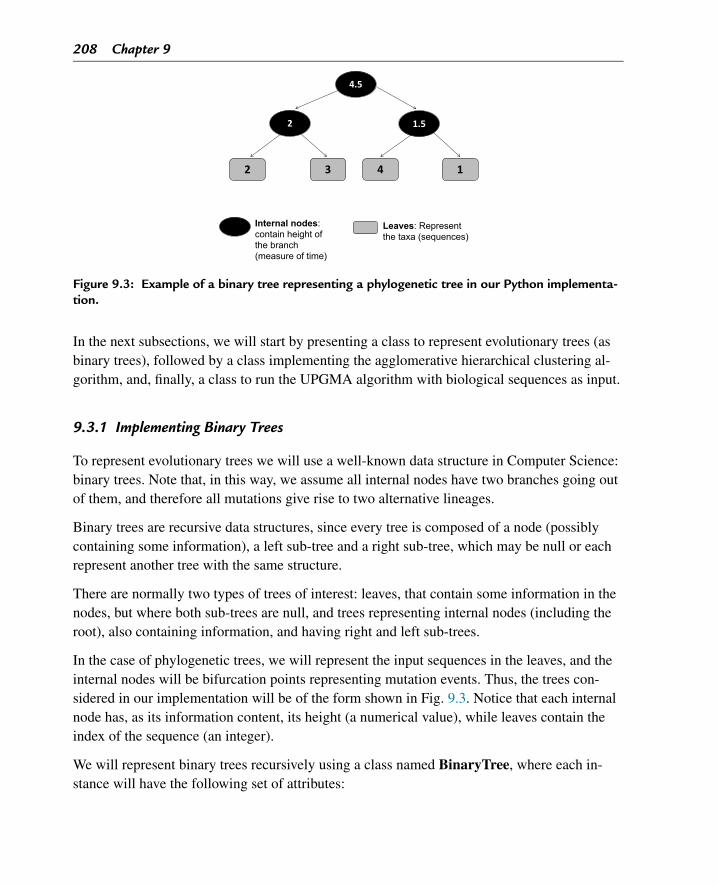
208 Chapter 9

Figure 9.3: Example of a binary tree representing a phylogenetic tree in our Python implementa-tion.

In the next subsections, we will start by presenting a class to represent evolutionary trees (asbinary trees), followed by a class implementing the agglomerative hierarchical clustering al-gorithm, and, finally, a class to run the UPGMA algorithm with biological sequences as input.

9.3.1 Implementing Binary Trees

To represent evolutionary trees we will use a well-known data structure in Computer Science:binary trees. Note that, in this way, we assume all internal nodes have two branches going outof them, and therefore all mutations give rise to two alternative lineages.

Binary trees are recursive data structures, since every tree is composed of a node (possiblycontaining some information), a left sub-tree and a right sub-tree, which may be null or eachrepresent another tree with the same structure.

There are normally two types of trees of interest: leaves, that contain some information in thenodes, but where both sub-trees are null, and trees representing internal nodes (including theroot), also containing information, and having right and left sub-trees.

In the case of phylogenetic trees, we will represent the input sequences in the leaves, and theinternal nodes will be bifurcation points representing mutation events. Thus, the trees con-sidered in our implementation will be of the form shown in Fig. 9.3. Notice that each internalnode has, as its information content, its height (a numerical value), while leaves contain theindex of the sequence (an integer).

We will represent binary trees recursively using a class named BinaryTree, where each in-stance will have the following set of attributes:

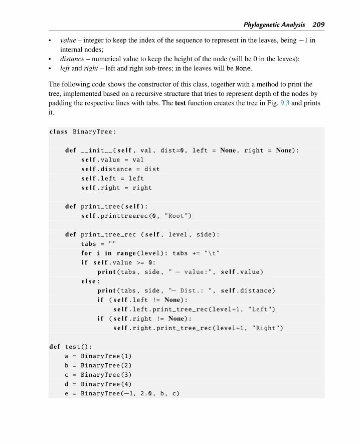
Phylogenetic Analysis 209

• value – integer to keep the index of the sequence to represent in the leaves, being −1 ininternal nodes;

• distance – numerical value to keep the height of the node (will be 0 in the leaves);• left and right – left and right sub-trees; in the leaves will be None.

The following code shows the constructor of this class, together with a method to print thetree, implemented based on a recursive structure that tries to represent depth of the nodes bypadding the respective lines with tabs. The test function creates the tree in Fig. 9.3 and printsit.

c l a s s BinaryTree:

def __init__( s e l f , val, dist=0, left = None, right = None):s e l f .value = vals e l f .distance = dists e l f .left = lefts e l f .right = right

def print_tree( s e l f ):s e l f .printtreerec(0, "Root")

def print_tree_rec ( s e l f , level, side):tabs = ""

f o r i in range(level): tabs += "\t"i f s e l f .value >= 0:

p r i n t (tabs, side, " − value:", s e l f .value)e l s e :

p r i n t (tabs, side, "− Dist.: ", s e l f .distance)i f ( s e l f .left != None):

s e l f .left.print_tree_rec(level+1, "Left")i f ( s e l f .right != None):

s e l f .right.print_tree_rec(level+1, "Right")

def test():a = BinaryTree(1)

b = BinaryTree(2)

c = BinaryTree(3)

d = BinaryTree(4)

e = BinaryTree(−1, 2.0, b, c)

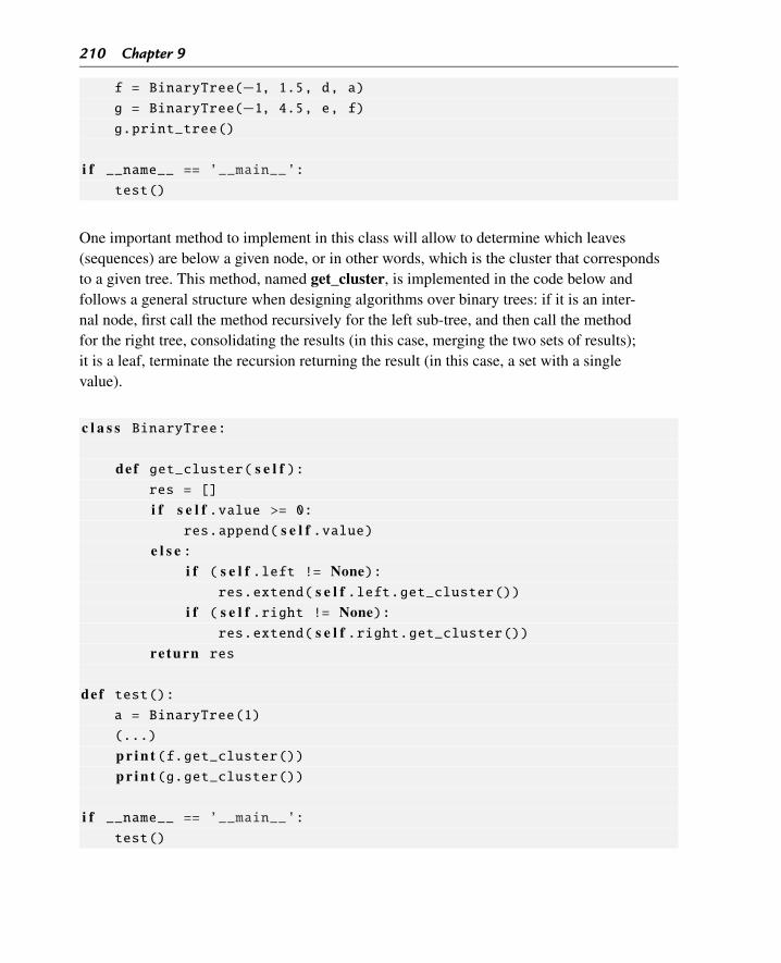
210 Chapter 9

f = BinaryTree(−1, 1.5, d, a)g = BinaryTree(−1, 4.5, e, f)g.print_tree()

i f __name__ == ’__main__’:test()

One important method to implement in this class will allow to determine which leaves(sequences) are below a given node, or in other words, which is the cluster that correspondsto a given tree. This method, named get_cluster, is implemented in the code below andfollows a general structure when designing algorithms over binary trees: if it is an inter-nal node, first call the method recursively for the left sub-tree, and then call the methodfor the right tree, consolidating the results (in this case, merging the two sets of results);it is a leaf, terminate the recursion returning the result (in this case, a set with a singlevalue).

c l a s s BinaryTree:

def get_cluster( s e l f ):res = []

i f s e l f .value >= 0:res.append( s e l f .value)

e l s e :i f ( s e l f .left != None):

res.extend( s e l f .left.get_cluster())i f ( s e l f .right != None):

res.extend( s e l f .right.get_cluster())re turn res

def test():a = BinaryTree(1)

(...)

p r i n t (f.get_cluster())p r i n t (g.get_cluster())

i f __name__ == ’__main__’:test()

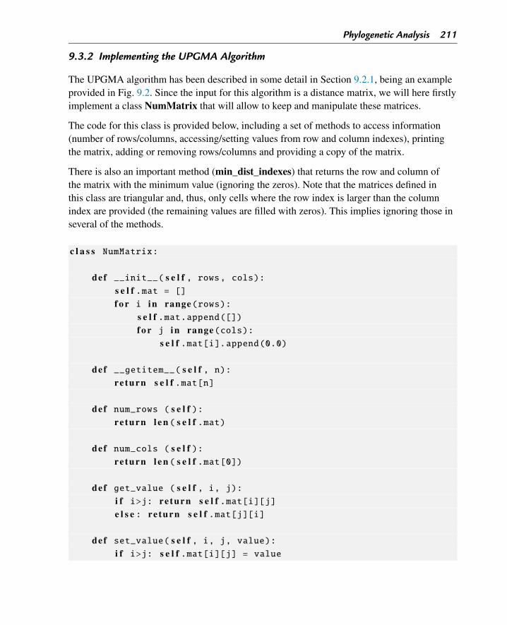
Phylogenetic Analysis 211

9.3.2 Implementing the UPGMA Algorithm

The UPGMA algorithm has been described in some detail in Section 9.2.1, being an exampleprovided in Fig. 9.2. Since the input for this algorithm is a distance matrix, we will here firstlyimplement a class NumMatrix that will allow to keep and manipulate these matrices.

The code for this class is provided below, including a set of methods to access information(number of rows/columns, accessing/setting values from row and column indexes), printingthe matrix, adding or removing rows/columns and providing a copy of the matrix.

There is also an important method (min_dist_indexes) that returns the row and column ofthe matrix with the minimum value (ignoring the zeros). Note that the matrices defined inthis class are triangular and, thus, only cells where the row index is larger than the columnindex are provided (the remaining values are filled with zeros). This implies ignoring those inseveral of the methods.

c l a s s NumMatrix:

def __init__( s e l f , rows, cols):s e l f .mat = []f o r i in range(rows):

s e l f .mat.append([])f o r j in range(cols):

s e l f .mat[i].append(0.0)

def __getitem__( s e l f , n):re turn s e l f .mat[n]

def num_rows ( s e l f ):re turn l e n ( s e l f .mat)

def num_cols ( s e l f ):re turn l e n ( s e l f .mat[0])

def get_value ( s e l f , i, j):i f i>j: re turn s e l f .mat[i][j]e l s e : re turn s e l f .mat[j][i]

def set_value( s e l f , i, j, value):i f i>j: s e l f .mat[i][j] = value

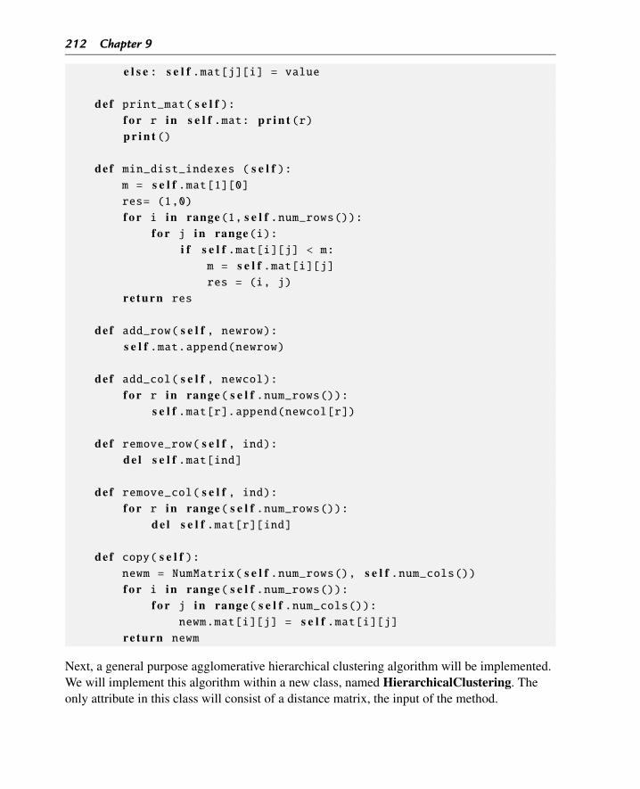
212 Chapter 9

e l s e : s e l f .mat[j][i] = value

def print_mat( s e l f ):f o r r in s e l f .mat: p r i n t (r)p r i n t ()

def min_dist_indexes ( s e l f ):m = s e l f .mat[1][0]res= (1,0)

f o r i in range(1, s e l f .num_rows()):f o r j in range(i):

i f s e l f .mat[i][j] < m:m = s e l f .mat[i][j]res = (i, j)

re turn res

def add_row( s e l f , newrow):s e l f .mat.append(newrow)

def add_col( s e l f , newcol):f o r r in range( s e l f .num_rows()):

s e l f .mat[r].append(newcol[r])

def remove_row( s e l f , ind):d e l s e l f .mat[ind]

def remove_col( s e l f , ind):f o r r in range( s e l f .num_rows()):

d e l s e l f .mat[r][ind]

def copy( s e l f ):newm = NumMatrix( s e l f .num_rows(), s e l f .num_cols())f o r i in range( s e l f .num_rows()):

f o r j in range( s e l f .num_cols()):newm.mat[i][j] = s e l f .mat[i][j]

re turn newm

Next, a general purpose agglomerative hierarchical clustering algorithm will be implemented.We will implement this algorithm within a new class, named HierarchicalClustering. Theonly attribute in this class will consist of a distance matrix, the input of the method.

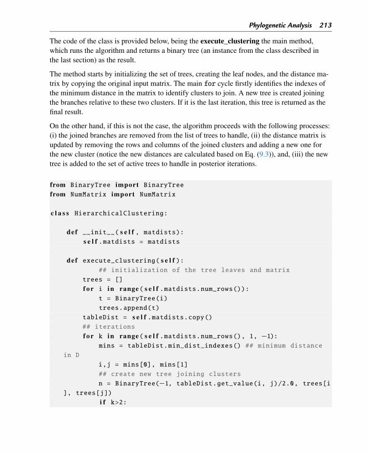
Phylogenetic Analysis 213

The code of the class is provided below, being the execute_clustering the main method,which runs the algorithm and returns a binary tree (an instance from the class described inthe last section) as the result.

The method starts by initializing the set of trees, creating the leaf nodes, and the distance ma-trix by copying the original input matrix. The main for cycle firstly identifies the indexes ofthe minimum distance in the matrix to identify clusters to join. A new tree is created joiningthe branches relative to these two clusters. If it is the last iteration, this tree is returned as thefinal result.

On the other hand, if this is not the case, the algorithm proceeds with the following processes:(i) the joined branches are removed from the list of trees to handle, (ii) the distance matrix isupdated by removing the rows and columns of the joined clusters and adding a new one forthe new cluster (notice the new distances are calculated based on Eq. (9.3)), and, (iii) the newtree is added to the set of active trees to handle in posterior iterations.

from BinaryTree import BinaryTreefrom NumMatrix import NumMatrix

c l a s s HierarchicalClustering:

def __init__( s e l f , matdists):s e l f .matdists = matdists

def execute_clustering( s e l f ):## initialization of the tree leaves and matrix

trees = []

f o r i in range( s e l f .matdists.num_rows()):t = BinaryTree(i)

trees.append(t)

tableDist = s e l f .matdists.copy()## iterations

f o r k in range( s e l f .matdists.num_rows(), 1, −1):mins = tableDist.min_dist_indexes() ## minimum distance

in D

i,j = mins[0], mins[1]

## create new tree joining clusters

n = BinaryTree(−1, tableDist.get_value(i, j)/2.0, trees[i], trees[j])

i f k>2:

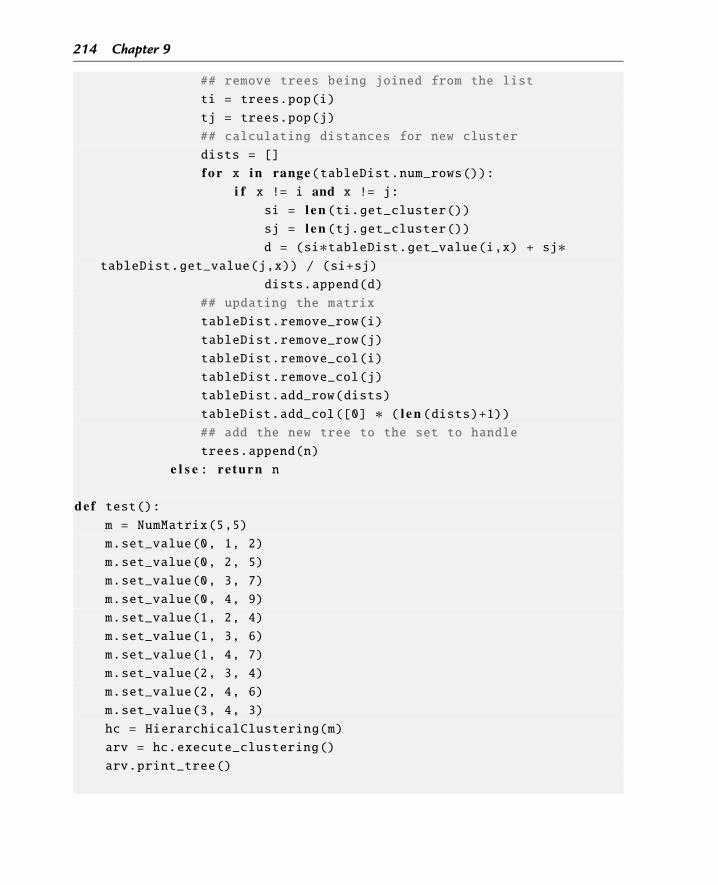
214 Chapter 9

## remove trees being joined from the list

ti = trees.pop(i)

tj = trees.pop(j)

## calculating distances for new cluster

dists = []

f o r x in range(tableDist.num_rows()):i f x != i and x != j:

si = l e n (ti.get_cluster())sj = l e n (tj.get_cluster())d = (si∗tableDist.get_value(i,x) + sj∗

tableDist.get_value(j,x)) / (si+sj)

dists.append(d)

## updating the matrix

tableDist.remove_row(i)

tableDist.remove_row(j)

tableDist.remove_col(i)

tableDist.remove_col(j)

tableDist.add_row(dists)

tableDist.add_col([0] ∗ ( l e n (dists)+1))## add the new tree to the set to handle

trees.append(n)

e l s e : re turn n

def test():m = NumMatrix(5,5)

m.set_value(0, 1, 2)

m.set_value(0, 2, 5)

m.set_value(0, 3, 7)

m.set_value(0, 4, 9)

m.set_value(1, 2, 4)

m.set_value(1, 3, 6)

m.set_value(1, 4, 7)

m.set_value(2, 3, 4)

m.set_value(2, 4, 6)

m.set_value(3, 4, 3)

hc = HierarchicalClustering(m)

arv = hc.execute_clustering()

arv.print_tree()

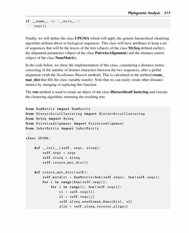
Phylogenetic Analysis 215

i f __name__ == ’__main__’:test()

Finally, we will define the class UPGMA which will apply the generic hierarchical clusteringalgorithm defined above to biological sequences. This class will have attributes to keep a setof sequences that will be the leaves of the tree (objects of the class MySeq defined earlier),the alignment parameters (object of the class PairwiseAlignment) and the distance matrix(object of the class NumMatrix).

In the code below, we show the implementation of this class, considering a distance metricconsisting of the number of distinct characters between the two sequences, after a globalalignment (with the Needleman-Wunsch method). This is calculated in the method create_mat_dist that fills the class variable matdist. Note that we can easily create other distancemetrics by changing or replacing this function.

The run method is used to create an object of the class HierarchicalClustering and executethe clustering algorithm, returning the resulting tree.

from NumMatrix import NumMatrixfrom HierarchicalClustering import HierarchicalClusteringfrom MySeq import MySeqfrom PairwiseAlignment import PairwiseAlignmentfrom SubstMatrix import SubstMatrix

c l a s s UPGMA:

def __init__( s e l f , seqs, alseq):s e l f .seqs = seqss e l f .alseq = alseqs e l f .create_mat_dist()

def create_mat_dist( s e l f ):s e l f .matdist = NumMatrix( l e n ( s e l f .seqs), l e n ( s e l f .seqs))f o r i in range( l e n ( s e l f .seqs)):

f o r j in range(i, l e n ( s e l f .seqs)):s1 = s e l f .seqs[i]s2 = s e l f .seqs[j]s e l f .alseq.needleman_Wunsch(s1, s2)alin = s e l f .alseq.recover_align()

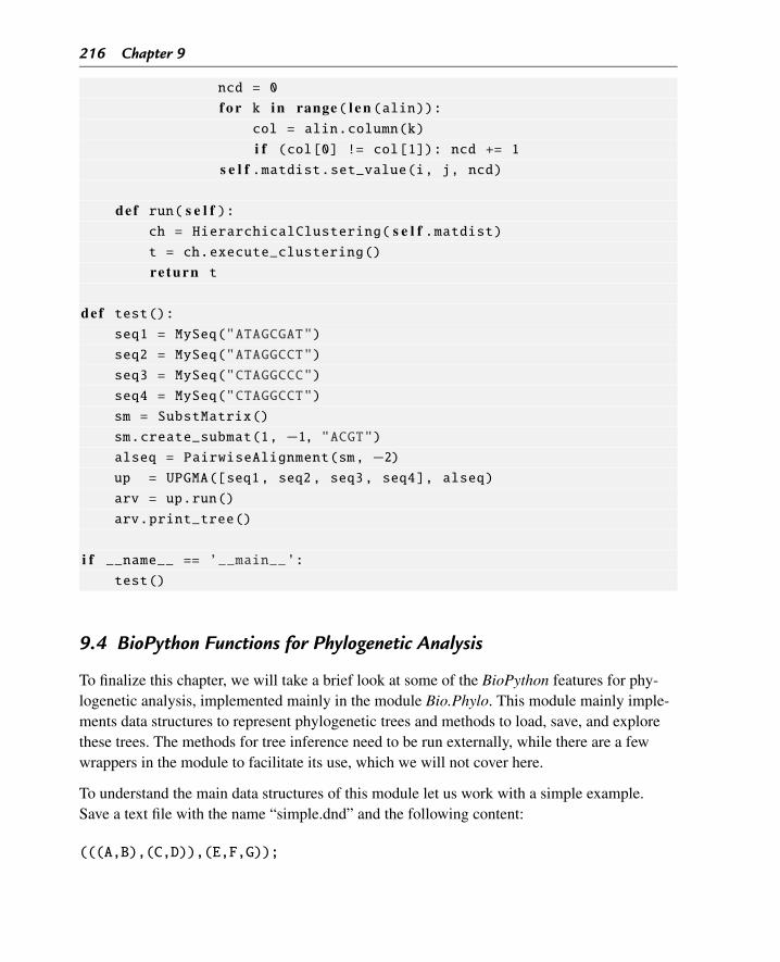
216 Chapter 9

ncd = 0

f o r k in range( l e n (alin)):col = alin.column(k)

i f (col[0] != col[1]): ncd += 1s e l f .matdist.set_value(i, j, ncd)

def run( s e l f ):ch = HierarchicalClustering( s e l f .matdist)t = ch.execute_clustering()

re turn t

def test():seq1 = MySeq("ATAGCGAT")

seq2 = MySeq("ATAGGCCT")

seq3 = MySeq("CTAGGCCC")

seq4 = MySeq("CTAGGCCT")

sm = SubstMatrix()

sm.create_submat(1, −1, "ACGT")alseq = PairwiseAlignment(sm, −2)up = UPGMA([seq1, seq2, seq3, seq4], alseq)

arv = up.run()

arv.print_tree()

i f __name__ == ’__main__’:test()

9.4 BioPython Functions for Phylogenetic Analysis

To finalize this chapter, we will take a brief look at some of the BioPython features for phy-logenetic analysis, implemented mainly in the module Bio.Phylo. This module mainly imple-ments data structures to represent phylogenetic trees and methods to load, save, and explorethese trees. The methods for tree inference need to be run externally, while there are a fewwrappers in the module to facilitate its use, which we will not cover here.

To understand the main data structures of this module let us work with a simple example.Save a text file with the name “simple.dnd” and the following content:

(((A,B),(C,D)),(E,F,G));

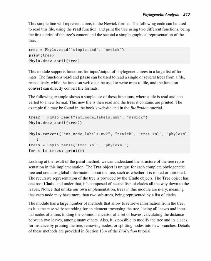
Phylogenetic Analysis 217

This simple line will represent a tree, in the Newick format. The following code can be usedto read this file, using the read function, and print the tree using two different functions, beingthe first a print of the tree’s content and the second a simple graphical representation of thetree.

tree = Phylo.read("simple.dnd", "newick")

p r i n t (tree)Phylo.draw_ascii(tree)

This module supports functions for input/output of phylogenetic trees in a large list of for-mats. The functions read and parse can be used to read a single or several trees from a file,respectively, while the function write can be used to write trees to file, and the functionconvert can directly convert file formats.

The following example shows a simple use of these functions, where a file is read and con-verted to a new format. This new file is then read and the trees it contains are printed. Theexample file may be found in the book’s website and in the BioPython tutorial.

tree2 = Phylo.read("int_node_labels.nwk", "newick")

Phylo.draw_ascii(tree2)

Phylo.convert("int_node_labels.nwk", "newick", "tree.xml", "phyloxml"

)

trees = Phylo.parse("tree.xml", "phyloxml")

f o r t in trees: p r i n t (t)

Looking at the result of the print method, we can understand the structure of the tree repre-sentation in this implementation. The Tree object is unique for each complete phylogenetictree and contains global information about the tree, such as whether it is rooted or unrooted.The recursive representation of the tree is provided by the Clade objects. The Tree object hasone root Clade, and under that, it’s composed of nested lists of clades all the way down to theleaves. Notice that unlike our own implementation, trees in this module are n-ary, meaningthat each node may have more than two sub-trees, being represented by a list of clades.

The module has a large number of methods that allow to retrieve information from the tree,as it is the case with: searching for an element traversing the tree, listing all leaves and inter-nal nodes of a tree, finding the common ancestor of a set of leaves, calculating the distancebetween two leaves, among many others. Also, it is possible to modify the tree and its clades,for instance by pruning the tree, removing nodes, or splitting nodes into new branches. Detailsof these methods are provided in Section 13.4 of the BioPython tutorial.

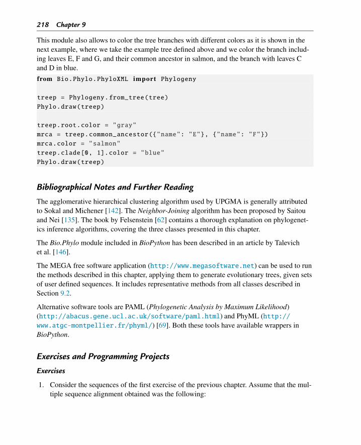
218 Chapter 9

This module also allows to color the tree branches with different colors as it is shown in thenext example, where we take the example tree defined above and we color the branch includ-ing leaves E, F and G, and their common ancestor in salmon, and the branch with leaves Cand D in blue.

from Bio.Phylo.PhyloXML import Phylogeny

treep = Phylogeny.from_tree(tree)

Phylo.draw(treep)

treep.root.color = "gray"

mrca = treep.common_ancestor({"name": "E"}, {"name": "F"})

mrca.color = "salmon"

treep.clade[0, 1].color = "blue"

Phylo.draw(treep)

Bibliographical Notes and Further Reading

The agglomerative hierarchical clustering algorithm used by UPGMA is generally attributedto Sokal and Michener [142]. The Neighbor-Joining algorithm has been proposed by Saitouand Nei [135]. The book by Felsenstein [62] contains a thorough explanation on phylogenet-ics inference algorithms, covering the three classes presented in this chapter.

The Bio.Phylo module included in BioPython has been described in an article by Talevichet al. [146].

The MEGA free software application (http://www.megasoftware.net) can be used to runthe methods described in this chapter, applying them to generate evolutionary trees, given setsof user defined sequences. It includes representative methods from all classes described inSection 9.2.

Alternative software tools are PAML (Phylogenetic Analysis by Maximum Likelihood)(http://abacus.gene.ucl.ac.uk/software/paml.html) and PhyML (http://www.atgc-montpellier.fr/phyml/) [69]. Both these tools have available wrappers inBioPython.

Exercises and Programming Projects

Exercises

1. Consider the sequences of the first exercise of the previous chapter. Assume that the mul-tiple sequence alignment obtained was the following:

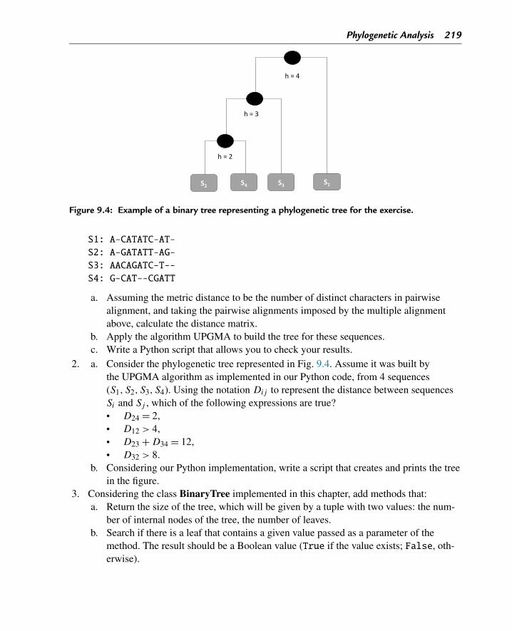
Phylogenetic Analysis 219

Figure 9.4: Example of a binary tree representing a phylogenetic tree for the exercise.

S1: A-CATATC-AT-S2: A-GATATT-AG-S3: AACAGATC-T--S4: G-CAT--CGATT

a. Assuming the metric distance to be the number of distinct characters in pairwisealignment, and taking the pairwise alignments imposed by the multiple alignmentabove, calculate the distance matrix.

b. Apply the algorithm UPGMA to build the tree for these sequences.c. Write a Python script that allows you to check your results.

2. a. Consider the phylogenetic tree represented in Fig. 9.4. Assume it was built bythe UPGMA algorithm as implemented in our Python code, from 4 sequences(S1, S2, S3, S4). Using the notation Dij to represent the distance between sequencesSi and Sj , which of the following expressions are true?• D24 = 2,• D12 > 4,• D23 + D34 = 12,• D32 > 8.

b. Considering our Python implementation, write a script that creates and prints the treein the figure.

3. Considering the class BinaryTree implemented in this chapter, add methods that:a. Return the size of the tree, which will be given by a tuple with two values: the num-

ber of internal nodes of the tree, the number of leaves.b. Search if there is a leaf that contains a given value passed as a parameter of the

method. The result should be a Boolean value (True if the value exists; False, oth-erwise).

220 Chapter 9

c. Return the common ancestor of two sequences/taxa (identified as integer values),i.e. will return the simplest tree (with less height) that contains the leaves with thosevalues.

d. Generalize the previous function to a set of sequences as input.e. Return the distance between two leaves identified by their integer values.f. Return the distance between the two leaves (identified by their integer values) that

are nearest in the tree (i.e. have their common ancestor at the smallest height).4. Implement the WPGMA variant of the UPGMA algorithm, changing the way the dis-

tance between clusters is calculated (as described above). Compare the results of bothapproaches.

5. Consider the last exercise of the previous chapter. Read the tree obtained from ClustalOmega. Draw the tree with the Bio.Phylo module. Explore the tree using the availablefunctions.

Programming Projects

1. Implement the Neighbor-Joining method applied to rooted trees, as described above inSection 9.2.1.

2. Extend the class UPGMA, by considering other distance metrics for the sequences (e.g.edit distance). Take into account the sequence type (nucleotide vs protein) to definemeaningful metrics.

3. Implement a simple maximum parsimony method, by firstly creating a multiple sequencealignment of the sequences. Add a function to identify informative columns (where thereare mutations). Implement a cost function for a tree, taking those columns into account.

CHAPTER 10

Motif Discovery AlgorithmsIn this chapter, we revisit and formalize the definition of deterministic motif. We introduce theconcept of search and solution space and formally define the problem of deterministic motifsearch in a set of biologically related sequences. We start by describing brute-force algorithmsbased on an exhaustive search and then present more efficient approaches for motif discovery.

10.1 Introduction: Problem Definition and Relevance

Within the context of biological sequence mining, the term motif refers to a non-trivial se-quential pattern that is shared across multiple sequences. With non-trivial, we mean that themotif has a minimum relevant length and captures a combination of symbols that differs fromthe underlying symbol distribution. However, its main feature is its recurrence, i.e. the factthat it occurs in several of the analyzed sequences.

The relevance of a motif arises when the set of sequences where it occurs are associated to ge-nomic elements, such as genes, that share a certain biological property or are under the sameregulatory control. The hypothesis will then be that the motif will play a role in the associatedbiological phenomenon.

For instance, in DNA sequences, motifs may occur in the promoter region of genes and in-dicate the presence of binding sites of single proteins or protein complexes that have a regu-latory role in gene transcription. In protein sequences, motifs may indicate the existence ofconserved domains, i.e. parts of the protein that play specific biological functions, such as en-zyme binding sites for substrates or other molecules.

We can distinguish two main classes of motifs: deterministic and probabilistic. Deterministicmotifs are often captured by enhanced regular expression syntax, and as it name indicates areeither present or absent in the input sequences. These were already addressed in the context ofChapter 5.

On the other hand, probabilistic motifs form a loose model that captures the underlying vari-ability of the motif occurrences. When a given segment of a sequence is presented to themodel, the probability of being part of the motif can be derived. As we will see in the nextchapter, position weight matrices (PWMs) can be used as a way to represent probabilistic mo-tifs. In this chapter, we will discuss the algorithmic framework to define deterministic motifsand present motif finding algorithms with increasing efficiency level.

Bioinformatics Algorithms. DOI: 10.1016/B978-0-12-812520-5.00010-9Copyright © 2018 Elsevier Inc. All rights reserved. 221

222 Chapter 10

We will start by introducing the concepts that will help us to better define the problem ofefficiently discovering the sequence motifs conserved among a set of related biological se-quences. Note that we will use the terms sequence pattern and motif with equivalent meaningthroughout this chapter.

As we have seen in previous chapters, biological sequences are defined as strings of symbols,which for DNA consist of four letters �DNA = {A,C,G,T } and for protein sequences oftwenty letters, �Protein = {A,C,D,E,F,G,H, I,K,L,M,N , P,Q,R,S,T ,V,W,Y }. Thecharacteristics of nucleotide sequences and proteins, such as the size of the alphabet, the typ-ical length of the sequence or the underlying symbol distribution raises different algorithmicchallenges. Therefore, motif discovery algorithms need to be optimized according to the na-ture of sequences to which they are applied.

As we mentioned before, a deterministic motif can be captured by regular expression syn-tax. In some cases, the motif is composed by a continuous combination of symbols, while inother more complex cases the motif may contain certain parts, possibly of variable length,corresponding to highly variable symbols, which apart from their length do not add any rele-vant information. These two cases can be differentiated using the terms, sub-string and sub-sequence. As defined in [70], a sub-string corresponds to a consecutive part of a string, whilea sub-sequence corresponds to a new sequence obtained by eventually dropping some sym-bols from the original sequence and preserving the respective order. The later is a more gen-eral case than the former. For instance, for a sequence S = abcdef , acdf is a sub-sequence ofS and bcd is a sub-string of S.

If |S| denotes the length of the sequence S and S = xyz, |x| ≥ 0 and |z| ≥ 0 then x is said tobe a prefix of S and y is suffix of S. Alternatively, S is a superstring or supersequence of x.

Generally, a deterministic motif M can be defined as a non-null string of symbols from an en-hanced alphabet �′. The alphabet �′ results from an extension of � with an additional set ofsymbols E, �′ = � ∩ E. E adds greater expressiveness to the patterns and may contain sym-bols that express the existence of gaps or symbols that reflect positions that may be occupiedby more than one symbol. The set of all the possible regular expressions that result from thesubstitution of symbols from �′ in M defines a pattern language: L(M). A motif M is said tomatch or hit a sequence S, if S contains some string y that occurs in L(M).

We have seen in Chapter 5 that the restriction enzyme EcoRI cuts the DNA when it findsthe sequence pattern GAAT T C. In this case, we have a very clear pattern represented by aunique string. However, it is often the case that the binding sequences change slightly. Thisleads to more subtle patterns that need to comprise more than one sequence match. This is, forinstance, the case of HindII [140], a type II restriction enzyme that cuts the DNA in specificsequences that are six nucleotides long. When the DNA is read from the 5’ to 3’ sense, the

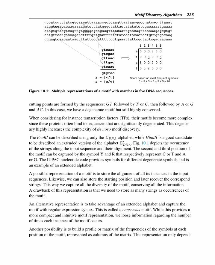
Motif Discovery Algorithms 223

Figure 10.1: Multiple representations of a motif with matches in five DNA sequences.

cutting points are formed by the sequences: GT followed by T or C, then followed by A or G

and AC. In this case, we have a degenerate motif but still highly conserved.

When considering for instance transcription factors (TFs), their motifs become more complexsince these proteins often bind to sequences that are significantly degenerated. This degener-acy highly increases the complexity of de novo motif discovery.

The EcoRI can be described using only the �DNA alphabet, while HindII is a good candidateto be described an extended version of the alphabet �′

DNA. Fig. 10.1 depicts the occurrenceof the strings along the input sequence and their alignment. The second and third position ofthe motif can be captured by the symbol Y and R that respectively represent C or T and Aor G. The IUPAC nucleotide code provides symbols for different degenerate symbols and isan example of an extended alphabet.

A possible representation of a motif is to store the alignment of all its instances in the inputsequences. Likewise, we can also store the starting position and later recover the correspondstrings. This way we capture all the diversity of the motif, conserving all the information.A drawback of this representation is that we need to store as many strings as occurrences ofthe motif.

An alternative representation is to take advantage of an extended alphabet and capture themotif with regular expression syntax. This is called a consensus motif. While this provides amore compact and intuitive motif representation, we loose information regarding the numberof times each instance of the motif occurs.

Another possibility is to build a profile or matrix of the frequencies of the symbols at eachposition of the motif, represented as columns of the matrix. This representation only depends

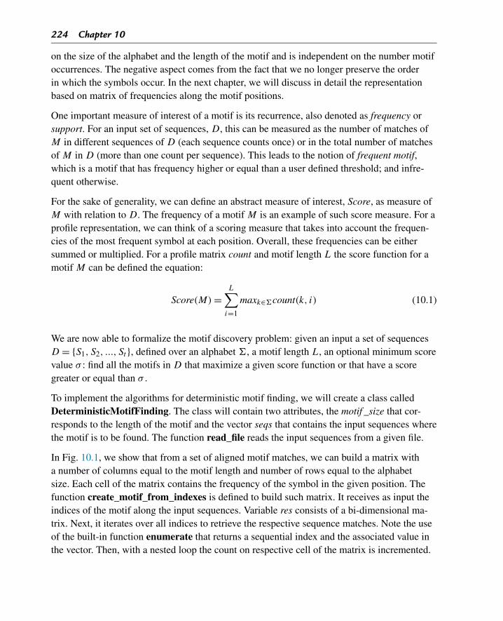
224 Chapter 10

on the size of the alphabet and the length of the motif and is independent on the number motifoccurrences. The negative aspect comes from the fact that we no longer preserve the orderin which the symbols occur. In the next chapter, we will discuss in detail the representationbased on matrix of frequencies along the motif positions.

One important measure of interest of a motif is its recurrence, also denoted as frequency orsupport. For an input set of sequences, D, this can be measured as the number of matches ofM in different sequences of D (each sequence counts once) or in the total number of matchesof M in D (more than one count per sequence). This leads to the notion of frequent motif,which is a motif that has frequency higher or equal than a user defined threshold; and infre-quent otherwise.

For the sake of generality, we can define an abstract measure of interest, Score, as measure ofM with relation to D. The frequency of a motif M is an example of such score measure. For aprofile representation, we can think of a scoring measure that takes into account the frequen-cies of the most frequent symbol at each position. Overall, these frequencies can be eithersummed or multiplied. For a profile matrix count and motif length L the score function for amotif M can be defined the equation:

Score(M) =L∑

i=1

maxk∈�count(k, i) (10.1)

We are now able to formalize the motif discovery problem: given an input a set of sequencesD = {S1, S2, ..., St }, defined over an alphabet �, a motif length L, an optional minimum scorevalue σ : find all the motifs in D that maximize a given score function or that have a scoregreater or equal than σ .

To implement the algorithms for deterministic motif finding, we will create a class calledDeterministicMotifFinding. The class will contain two attributes, the motif _size that cor-responds to the length of the motif and the vector seqs that contains the input sequences wherethe motif is to be found. The function read_file reads the input sequences from a given file.

In Fig. 10.1, we show that from a set of aligned motif matches, we can build a matrix witha number of columns equal to the motif length and number of rows equal to the alphabetsize. Each cell of the matrix contains the frequency of the symbol in the given position. Thefunction create_motif_from_indexes is defined to build such matrix. It receives as input theindices of the motif along the input sequences. Variable res consists of a bi-dimensional ma-trix. Next, it iterates over all indices to retrieve the respective sequence matches. Note the useof the built-in function enumerate that returns a sequential index and the associated value inthe vector. Then, with a nested loop the count on respective cell of the matrix is incremented.

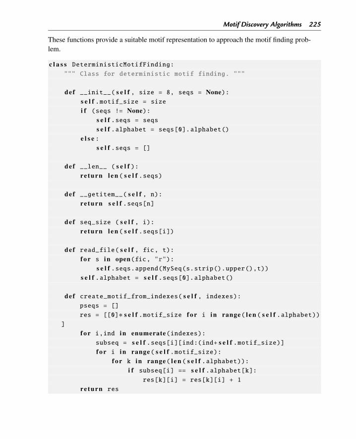
Motif Discovery Algorithms 225

These functions provide a suitable motif representation to approach the motif finding prob-lem.

c l a s s DeterministicMotifFinding:""" Class for deterministic motif finding. """

def __init__( s e l f , size = 8, seqs = None):s e l f .motif_size = sizei f (seqs != None):

s e l f .seqs = seqss e l f .alphabet = seqs[0].alphabet()

e l s e :s e l f .seqs = []

def __len__ ( s e l f ):re turn l e n ( s e l f .seqs)

def __getitem__( s e l f , n):re turn s e l f .seqs[n]

def seq_size ( s e l f , i):re turn l e n ( s e l f .seqs[i])

def read_file( s e l f , fic, t):f o r s in open(fic, "r"):

s e l f .seqs.append(MySeq(s.strip().upper(),t))s e l f .alphabet = s e l f .seqs[0].alphabet()

def create_motif_from_indexes( s e l f , indexes):pseqs = []

res = [[0]∗ s e l f .motif_size f o r i in range( l e n ( s e l f .alphabet))]

f o r i,ind in enumerate(indexes):subseq = s e l f .seqs[i][ind:(ind+ s e l f .motif_size)]f o r i in range( s e l f .motif_size):

f o r k in range( l e n ( s e l f .alphabet)):i f subseq[i] == s e l f .alphabet[k]:

res[k][i] = res[k][i] + 1

re turn res

226 Chapter 10

The function score defined below implements the scoring function defined in Eq. (10.1). Thisfunction iterates through all the positions of the motif and, for each position, determines themaximum value which is added to the score of the motif. The function score_multiplicativeimplements a similar scoring, but instead of summing, the score is obtained by multiplyingthe maximum value at each motif position.

def score( s e l f , s):score = 0

mat = s e l f .create_motif_from_indexes(s)f o r j in range( l e n (mat[0])):

maxcol = mat[0][j]

f o r i in range(1, l e n (mat)):i f mat[i][j] > maxcol:

maxcol = mat[i][j]

score += maxcol

re turn score

def score_multiplicative( s e l f , s):score = 1.0

mat = s e l f .create_motif_from_indexes(s)f o r j in range( l e n (mat[0])):

maxcol = mat[0][j]

f o r i in range(1, l e n (mat)):i f mat[i][j] > maxcol:

maxcol = mat[i][j]

score ∗= maxcolre turn score

10.2 Brute-Force Algorithms: Exhaustive Search

To tackle the motif discovery problem as described in the previous section, we need to im-plement a solution that finds the vector s with the best initial positions of the motif in eachsequence. The algorithm will be defined as:

• Inputs: t – sequences (length n); L – length of motif; and σ – optional minimum score.• Outputs: A vector with the initial positions s = (s1, s2, ..., st ) of the motif M in D that

maximize the Score(s,D).

We can devise a solution based on an exhaustive search for the best positions. Since the goalis to maximize Score(s,D), we can scan all possible vectors of initial positions and calculate

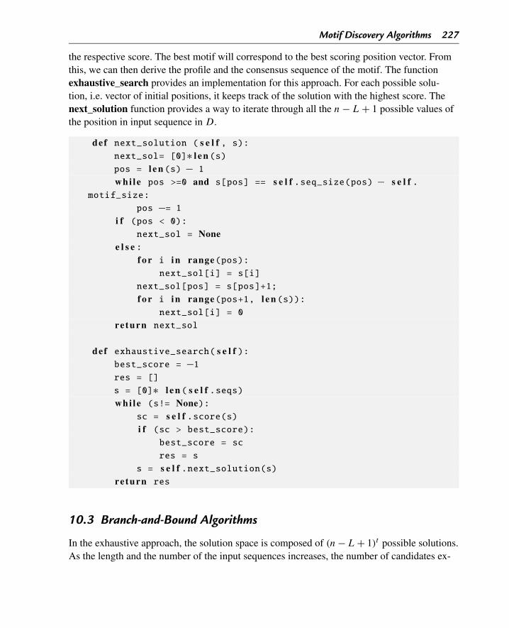
Motif Discovery Algorithms 227

the respective score. The best motif will correspond to the best scoring position vector. Fromthis, we can then derive the profile and the consensus sequence of the motif. The functionexhaustive_search provides an implementation for this approach. For each possible solu-tion, i.e. vector of initial positions, it keeps track of the solution with the highest score. Thenext_solution function provides a way to iterate through all the n − L + 1 possible values ofthe position in input sequence in D.

def next_solution ( s e l f , s):next_sol= [0]∗ l e n (s)pos = l e n (s) − 1

whi le pos >=0 and s[pos] == s e l f .seq_size(pos) − s e l f .motif_size:

pos −= 1i f (pos < 0):

next_sol = Nonee l s e :

f o r i in range(pos):next_sol[i] = s[i]

next_sol[pos] = s[pos]+1;

f o r i in range(pos+1, l e n (s)):next_sol[i] = 0

re turn next_sol

def exhaustive_search( s e l f ):best_score = −1res = []

s = [0]∗ l e n ( s e l f .seqs)whi le (s!= None):

sc = s e l f .score(s)i f (sc > best_score):

best_score = sc

res = s

s = s e l f .next_solution(s)re turn res

10.3 Branch-and-Bound Algorithms

In the exhaustive approach, the solution space is composed of (n − L + 1)t possible solutions.As the length and the number of the input sequences increases, the number of candidates ex-

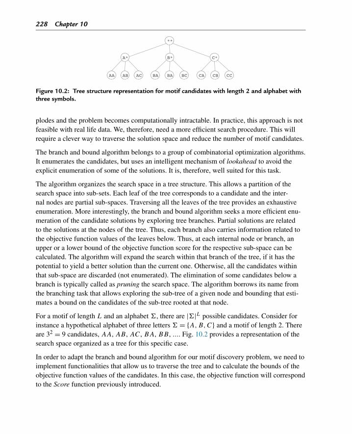
228 Chapter 10

Figure 10.2: Tree structure representation for motif candidates with length 2 and alphabet withthree symbols.

plodes and the problem becomes computationally intractable. In practice, this approach is notfeasible with real life data. We, therefore, need a more efficient search procedure. This willrequire a clever way to traverse the solution space and reduce the number of motif candidates.

The branch and bound algorithm belongs to a group of combinatorial optimization algorithms.It enumerates the candidates, but uses an intelligent mechanism of lookahead to avoid theexplicit enumeration of some of the solutions. It is, therefore, well suited for this task.

The algorithm organizes the search space in a tree structure. This allows a partition of thesearch space into sub-sets. Each leaf of the tree corresponds to a candidate and the inter-nal nodes are partial sub-spaces. Traversing all the leaves of the tree provides an exhaustiveenumeration. More interestingly, the branch and bound algorithm seeks a more efficient enu-meration of the candidate solutions by exploring tree branches. Partial solutions are relatedto the solutions at the nodes of the tree. Thus, each branch also carries information related tothe objective function values of the leaves below. Thus, at each internal node or branch, anupper or a lower bound of the objective function score for the respective sub-space can becalculated. The algorithm will expand the search within that branch of the tree, if it has thepotential to yield a better solution than the current one. Otherwise, all the candidates withinthat sub-space are discarded (not enumerated). The elimination of some candidates below abranch is typically called as pruning the search space. The algorithm borrows its name fromthe branching task that allows exploring the sub-tree of a given node and bounding that esti-mates a bound on the candidates of the sub-tree rooted at that node.

For a motif of length L and an alphabet �, there are |�|L possible candidates. Consider forinstance a hypothetical alphabet of three letters � = {A,B,C} and a motif of length 2. Thereare 32 = 9 candidates, AA, AB , AC, BA, BB , .... Fig. 10.2 provides a representation of thesearch space organized as a tree for this specific case.

In order to adapt the branch and bound algorithm for our motif discovery problem, we need toimplement functionalities that allow us to traverse the tree and to calculate the bounds of theobjective function values of the candidates. In this case, the objective function will correspondto the Score function previously introduced.

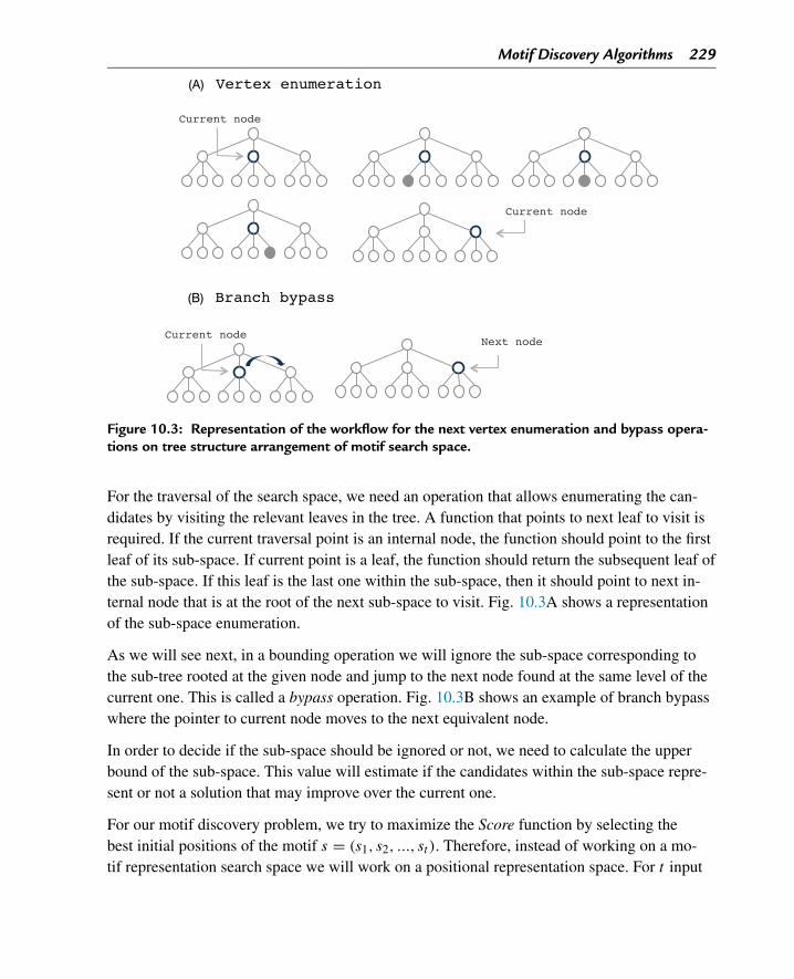
Motif Discovery Algorithms 229

Figure 10.3: Representation of the workflow for the next vertex enumeration and bypass opera-tions on tree structure arrangement of motif search space.

For the traversal of the search space, we need an operation that allows enumerating the can-didates by visiting the relevant leaves in the tree. A function that points to next leaf to visit isrequired. If the current traversal point is an internal node, the function should point to the firstleaf of its sub-space. If current point is a leaf, the function should return the subsequent leaf ofthe sub-space. If this leaf is the last one within the sub-space, then it should point to next in-ternal node that is at the root of the next sub-space to visit. Fig. 10.3A shows a representationof the sub-space enumeration.

As we will see next, in a bounding operation we will ignore the sub-space corresponding tothe sub-tree rooted at the given node and jump to the next node found at the same level of thecurrent one. This is called a bypass operation. Fig. 10.3B shows an example of branch bypasswhere the pointer to current node moves to the next equivalent node.

In order to decide if the sub-space should be ignored or not, we need to calculate the upperbound of the sub-space. This value will estimate if the candidates within the sub-space repre-sent or not a solution that may improve over the current one.

For our motif discovery problem, we try to maximize the Score function by selecting thebest initial positions of the motif s = (s1, s2, ..., st ). Therefore, instead of working on a mo-tif representation search space we will work on a positional representation space. For t input

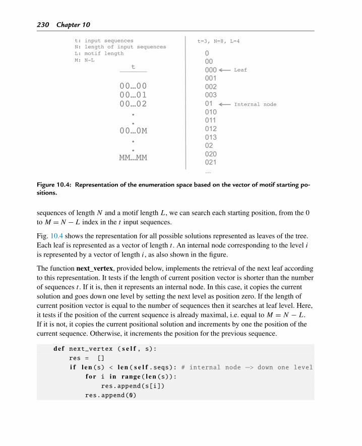
230 Chapter 10

Figure 10.4: Representation of the enumeration space based on the vector of motif starting po-sitions.

sequences of length N and a motif length L, we can search each starting position, from the 0to M = N − L index in the t input sequences.

Fig. 10.4 shows the representation for all possible solutions represented as leaves of the tree.Each leaf is represented as a vector of length t . An internal node corresponding to the level i

is represented by a vector of length i, as also shown in the figure.

The function next_vertex, provided below, implements the retrieval of the next leaf accordingto this representation. It tests if the length of current position vector is shorter than the numberof sequences t . If it is, then it represents an internal node. In this case, it copies the currentsolution and goes down one level by setting the next level as position zero. If the length ofcurrent position vector is equal to the number of sequences then it searches at leaf level. Here,it tests if the position of the current sequence is already maximal, i.e. equal to M = N − L.If it is not, it copies the current positional solution and increments by one the position of thecurrent sequence. Otherwise, it increments the position for the previous sequence.

def next_vertex ( s e l f , s):res = []

i f l e n (s) < l e n ( s e l f .seqs): # internal node −> down one levelf o r i in range( l e n (s)):

res.append(s[i])

res.append(0)

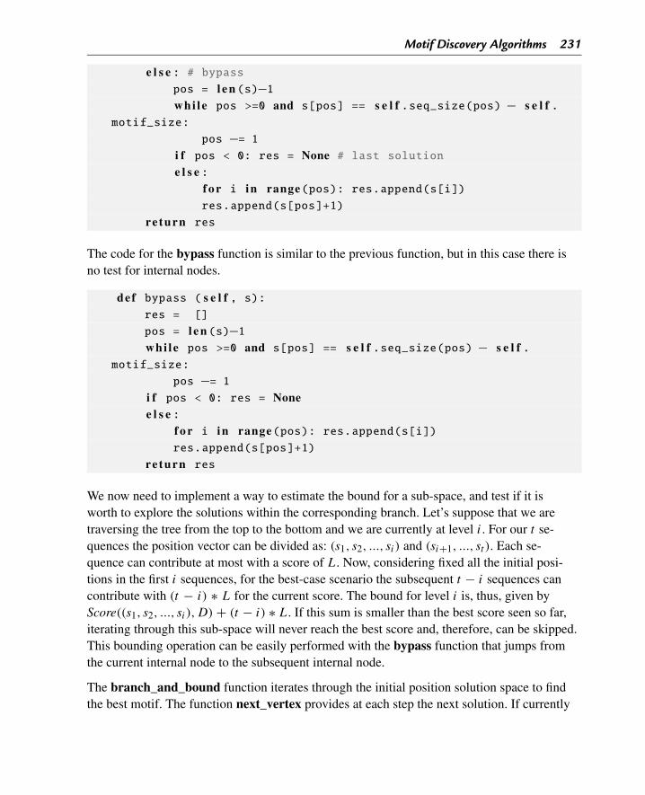
Motif Discovery Algorithms 231

e l s e : # bypasspos = l e n (s)−1whi le pos >=0 and s[pos] == s e l f .seq_size(pos) − s e l f .

motif_size:

pos −= 1i f pos < 0: res = None # last solutione l s e :

f o r i in range(pos): res.append(s[i])res.append(s[pos]+1)

re turn res

The code for the bypass function is similar to the previous function, but in this case there isno test for internal nodes.

def bypass ( s e l f , s):res = []

pos = l e n (s)−1whi le pos >=0 and s[pos] == s e l f .seq_size(pos) − s e l f .

motif_size:

pos −= 1i f pos < 0: res = Nonee l s e :

f o r i in range(pos): res.append(s[i])res.append(s[pos]+1)

re turn res

We now need to implement a way to estimate the bound for a sub-space, and test if it isworth to explore the solutions within the corresponding branch. Let’s suppose that we aretraversing the tree from the top to the bottom and we are currently at level i. For our t se-quences the position vector can be divided as: (s1, s2, ..., si) and (si+1, ..., st ). Each se-quence can contribute at most with a score of L. Now, considering fixed all the initial posi-tions in the first i sequences, for the best-case scenario the subsequent t − i sequences cancontribute with (t − i) ∗ L for the current score. The bound for level i is, thus, given byScore((s1, s2, ..., si),D) + (t − i) ∗ L. If this sum is smaller than the best score seen so far,iterating through this sub-space will never reach the best score and, therefore, can be skipped.This bounding operation can be easily performed with the bypass function that jumps fromthe current internal node to the subsequent internal node.

The branch_and_bound function iterates through the initial position solution space to findthe best motif. The function next_vertex provides at each step the next solution. If currently

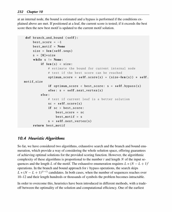
232 Chapter 10

at an internal node, the bound is estimated and a bypass is performed if the conditions ex-plained above are met. If positioned at a leaf, the current score is tested; if it exceeds the bestscore then the new best motif is updated to the current motif solution.

def branch_and_bound ( s e l f ):best_score = −1best_motif = Nonesize = l e n ( s e l f .seqs)s = [0]∗sizewhi le s != None:

i f l e n (s) < size:# estimate the bound for current internal node

# test if the best score can be reached

optimum_score = s e l f .score(s) + (size−l e n (s)) ∗ s e l f .motif_size

i f optimum_score < best_score: s = s e l f .bypass(s)e l s e : s = s e l f .next_vertex(s)

e l s e :# test if current leaf is a better solution

sc = s e l f .score(s)i f sc > best_score:

best_score = sc

best_motif = s

s = s e l f .next_vertex(s)re turn best_motif

10.4 Heuristic Algorithms

So far, we have considered two algorithms, exhaustive search and the branch and bound enu-meration, which provide a way of considering the whole solution space, offering guaranteesof achieving optimal solutions for the provided scoring function. However, the algorithmiccomplexity of these algorithms is proportional to the number t and length N of the input se-quences and the length L of the motif. The exhaustive enumeration requires L ∗ (N − L + 1)t

operations. In the branch and bound approach for i bypass operations, the search skipsL ∗ (N − L + 1)(t−i) candidates. In both cases, when the number of sequences reaches over10–12 and their length hundreds or thousands of symbols the problem becomes intractable.

In order to overcome this, heuristics have been introduced in different methods, with a trade-off between the optimality of the solution and computational efficiency. One of the earliest

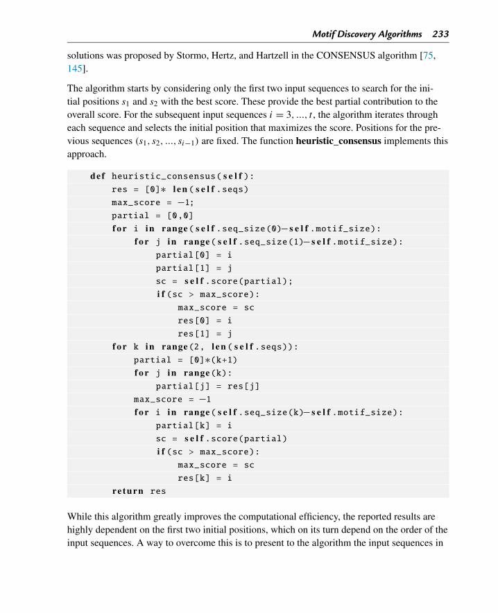
Motif Discovery Algorithms 233

solutions was proposed by Stormo, Hertz, and Hartzell in the CONSENSUS algorithm [75,145].

The algorithm starts by considering only the first two input sequences to search for the ini-tial positions s1 and s2 with the best score. These provide the best partial contribution to theoverall score. For the subsequent input sequences i = 3, ..., t , the algorithm iterates througheach sequence and selects the initial position that maximizes the score. Positions for the pre-vious sequences (s1, s2, ..., si−1) are fixed. The function heuristic_consensus implements thisapproach.

def heuristic_consensus( s e l f ):res = [0]∗ l e n ( s e l f .seqs)max_score = −1;partial = [0,0]

f o r i in range( s e l f .seq_size(0)−s e l f .motif_size):f o r j in range( s e l f .seq_size(1)−s e l f .motif_size):

partial[0] = i

partial[1] = j

sc = s e l f .score(partial);i f (sc > max_score):

max_score = sc

res[0] = i

res[1] = j

f o r k in range(2, l e n ( s e l f .seqs)):partial = [0]∗(k+1)f o r j in range(k):

partial[j] = res[j]

max_score = −1f o r i in range( s e l f .seq_size(k)−s e l f .motif_size):

partial[k] = i

sc = s e l f .score(partial)i f (sc > max_score):

max_score = sc

res[k] = i

re turn res

While this algorithm greatly improves the computational efficiency, the reported results arehighly dependent on the first two initial positions, which on its turn depend on the order of theinput sequences. A way to overcome this is to present to the algorithm the input sequences in

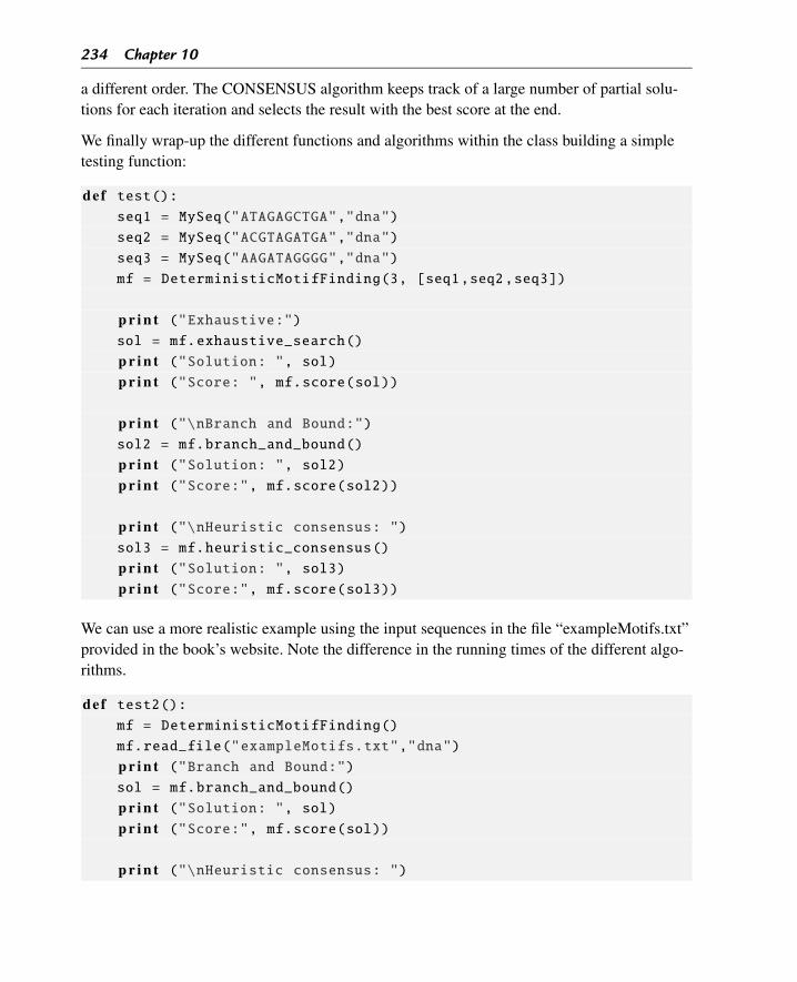
234 Chapter 10

a different order. The CONSENSUS algorithm keeps track of a large number of partial solu-tions for each iteration and selects the result with the best score at the end.

We finally wrap-up the different functions and algorithms within the class building a simpletesting function:

def test():seq1 = MySeq("ATAGAGCTGA","dna")

seq2 = MySeq("ACGTAGATGA","dna")

seq3 = MySeq("AAGATAGGGG","dna")

mf = DeterministicMotifFinding(3, [seq1,seq2,seq3])

p r i n t ("Exhaustive:")sol = mf.exhaustive_search()

p r i n t ("Solution: ", sol)p r i n t ("Score: ", mf.score(sol))

p r i n t ("\nBranch and Bound:")sol2 = mf.branch_and_bound()

p r i n t ("Solution: ", sol2)p r i n t ("Score:", mf.score(sol2))

p r i n t ("\nHeuristic consensus: ")sol3 = mf.heuristic_consensus()

p r i n t ("Solution: ", sol3)p r i n t ("Score:", mf.score(sol3))

We can use a more realistic example using the input sequences in the file “exampleMotifs.txt”provided in the book’s website. Note the difference in the running times of the different algo-rithms.

def test2():mf = DeterministicMotifFinding()

mf.read_file("exampleMotifs.txt","dna")

p r i n t ("Branch and Bound:")sol = mf.branch_and_bound()

p r i n t ("Solution: ", sol)p r i n t ("Score:", mf.score(sol))

p r i n t ("\nHeuristic consensus: ")

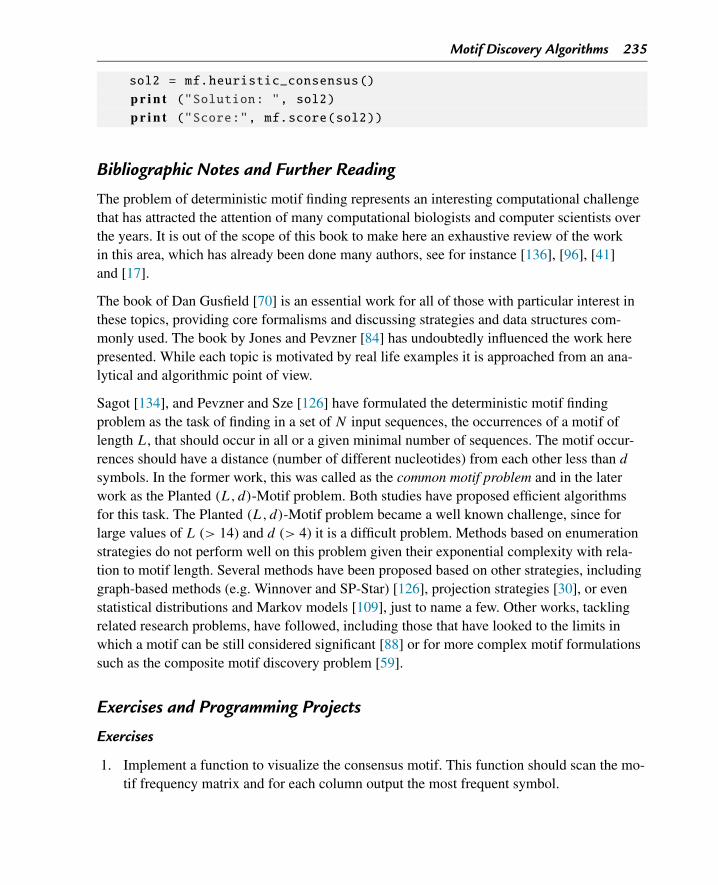
Motif Discovery Algorithms 235

sol2 = mf.heuristic_consensus()

p r i n t ("Solution: ", sol2)p r i n t ("Score:", mf.score(sol2))

Bibliographic Notes and Further Reading

The problem of deterministic motif finding represents an interesting computational challengethat has attracted the attention of many computational biologists and computer scientists overthe years. It is out of the scope of this book to make here an exhaustive review of the workin this area, which has already been done many authors, see for instance [136], [96], [41]and [17].

The book of Dan Gusfield [70] is an essential work for all of those with particular interest inthese topics, providing core formalisms and discussing strategies and data structures com-monly used. The book by Jones and Pevzner [84] has undoubtedly influenced the work herepresented. While each topic is motivated by real life examples it is approached from an ana-lytical and algorithmic point of view.

Sagot [134], and Pevzner and Sze [126] have formulated the deterministic motif findingproblem as the task of finding in a set of N input sequences, the occurrences of a motif oflength L, that should occur in all or a given minimal number of sequences. The motif occur-rences should have a distance (number of different nucleotides) from each other less than d

symbols. In the former work, this was called as the common motif problem and in the laterwork as the Planted (L, d)-Motif problem. Both studies have proposed efficient algorithmsfor this task. The Planted (L, d)-Motif problem became a well known challenge, since forlarge values of L (> 14) and d (> 4) it is a difficult problem. Methods based on enumerationstrategies do not perform well on this problem given their exponential complexity with rela-tion to motif length. Several methods have been proposed based on other strategies, includinggraph-based methods (e.g. Winnover and SP-Star) [126], projection strategies [30], or evenstatistical distributions and Markov models [109], just to name a few. Other works, tacklingrelated research problems, have followed, including those that have looked to the limits inwhich a motif can be still considered significant [88] or for more complex motif formulationssuch as the composite motif discovery problem [59].

Exercises and Programming Projects

Exercises

1. Implement a function to visualize the consensus motif. This function should scan the mo-tif frequency matrix and for each column output the most frequent symbol.

236 Chapter 10

2. Extend the previous function to include the IUPAC nucleotide ambiguity code. Forcolumns with multiple symbols use the corresponding symbol from IUPAC.

3. The result of the heuristic_consensus algorithm is highly dependent on the first two in-put sequences. Create a wrapper function that performs multiple iterations presenting theinput sequences in shuffled order and keep track of the resulting IUPAC consensus motifat each iteration.

Programming Projects

1. The motif finding algorithms presented in this chapter assume a one or more motif oc-currences per sequence. It can happen that the input set of sequences contain sequencesthat are not target of a motif (present in the rest of the sequences). Try to adapt the aboveimplementations to handle zero or more motif occurrences. The initial position vector fora sequence without a motif occurrence will have an offset of −1. One possible criteria todefine the absence of a motif hit in a sequence is that all its strings of length L have ap-proximately the same score. Thus, one could define a motif absence when the differencebetween the best scoring string and the worst scoring string is lower than a given thresh-old score.

2. Adapt the function implementing the CONSENSUS algorithm to be more robust, consid-ering at each stage several possible alternatives and exploring those in further iterations.Keep in each iteration a maximum of K alternatives, where K could be user-defined.

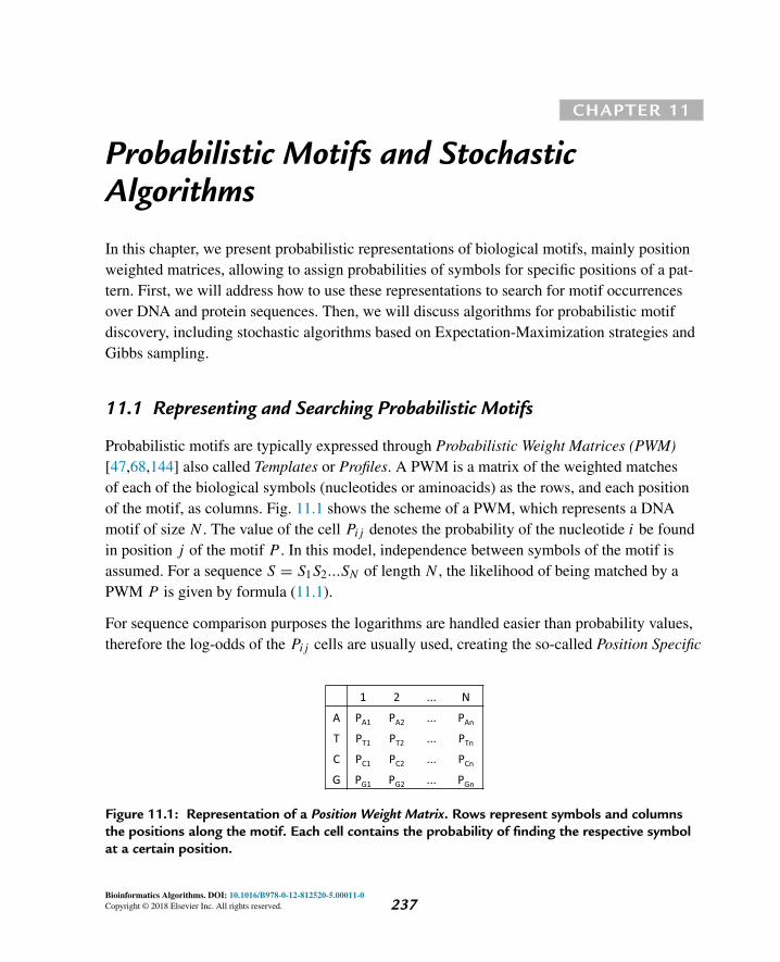
CHAPTER 11

Probabilistic Motifs and StochasticAlgorithms

In this chapter, we present probabilistic representations of biological motifs, mainly positionweighted matrices, allowing to assign probabilities of symbols for specific positions of a pat-tern. First, we will address how to use these representations to search for motif occurrencesover DNA and protein sequences. Then, we will discuss algorithms for probabilistic motifdiscovery, including stochastic algorithms based on Expectation-Maximization strategies andGibbs sampling.

11.1 Representing and Searching Probabilistic Motifs

Probabilistic motifs are typically expressed through Probabilistic Weight Matrices (PWM)[47,68,144] also called Templates or Profiles. A PWM is a matrix of the weighted matchesof each of the biological symbols (nucleotides or aminoacids) as the rows, and each positionof the motif, as columns. Fig. 11.1 shows the scheme of a PWM, which represents a DNAmotif of size N . The value of the cell Pij denotes the probability of the nucleotide i be foundin position j of the motif P . In this model, independence between symbols of the motif isassumed. For a sequence S = S1S2...SN of length N , the likelihood of being matched by aPWM P is given by formula (11.1).

For sequence comparison purposes the logarithms are handled easier than probability values,therefore the log-odds of the Pij cells are usually used, creating the so-called Position Specific

Figure 11.1: Representation of a Position Weight Matrix. Rows represent symbols and columnsthe positions along the motif. Each cell contains the probability of finding the respective symbolat a certain position.

Bioinformatics Algorithms. DOI: 10.1016/B978-0-12-812520-5.00011-0Copyright © 2018 Elsevier Inc. All rights reserved. 237

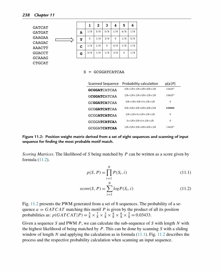
238 Chapter 11

Figure 11.2: Position weight matrix derived from a set of eight sequences and scanning of inputsequence for finding the most probable motif match.

Scoring Matrices. The likelihood of S being matched by P can be written as a score given byformula (11.2).

p(S,P ) =N∏

i=1

P(Si, i) (11.1)

score(S,P ) =N∑

i=1

logP(Si, i) (11.2)

Fig. 11.2 presents the PWM generated from a set of 8 sequences. The probability of a se-quence a = GAT CAT matching this motif P is given by the product of all its positionprobabilities as: p(GAT CAT |P) = 5

8 × 78 × 3

8 × 48 × 6

8 × 58 = 0.03433.

Given a sequence S and PWM P , we can calculate the sub-sequence of S with length N withthe highest likelihood of being matched by P . This can be done by scanning S with a slidingwindow of length N and applying the calculation as in formula (11.1). Fig. 11.2 describes theprocess and the respective probability calculation when scanning an input sequence.

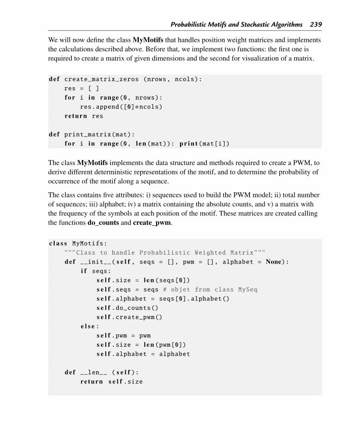
Probabilistic Motifs and Stochastic Algorithms 239

We will now define the class MyMotifs that handles position weight matrices and implementsthe calculations described above. Before that, we implement two functions: the first one isrequired to create a matrix of given dimensions and the second for visualization of a matrix.

def create_matrix_zeros (nrows, ncols):res = [ ]

f o r i in range(0, nrows):res.append([0]∗ncols)

re turn res

def print_matrix(mat):f o r i in range(0, l e n (mat)): p r i n t (mat[i])

The class MyMotifs implements the data structure and methods required to create a PWM, toderive different deterministic representations of the motif, and to determine the probability ofoccurrence of the motif along a sequence.

The class contains five attributes: i) sequences used to build the PWM model; ii) total numberof sequences; iii) alphabet; iv) a matrix containing the absolute counts, and v) a matrix withthe frequency of the symbols at each position of the motif. These matrices are created callingthe functions do_counts and create_pwm.

c l a s s MyMotifs:"""Class to handle Probabilistic Weighted Matrix"""

def __init__( s e l f , seqs = [], pwm = [], alphabet = None):i f seqs:

s e l f .size = l e n (seqs[0])s e l f .seqs = seqs # objet from class MySeqs e l f .alphabet = seqs[0].alphabet()s e l f .do_counts()s e l f .create_pwm()

e l s e :s e l f .pwm = pwms e l f .size = l e n (pwm[0])s e l f .alphabet = alphabet

def __len__ ( s e l f ):re turn s e l f .size

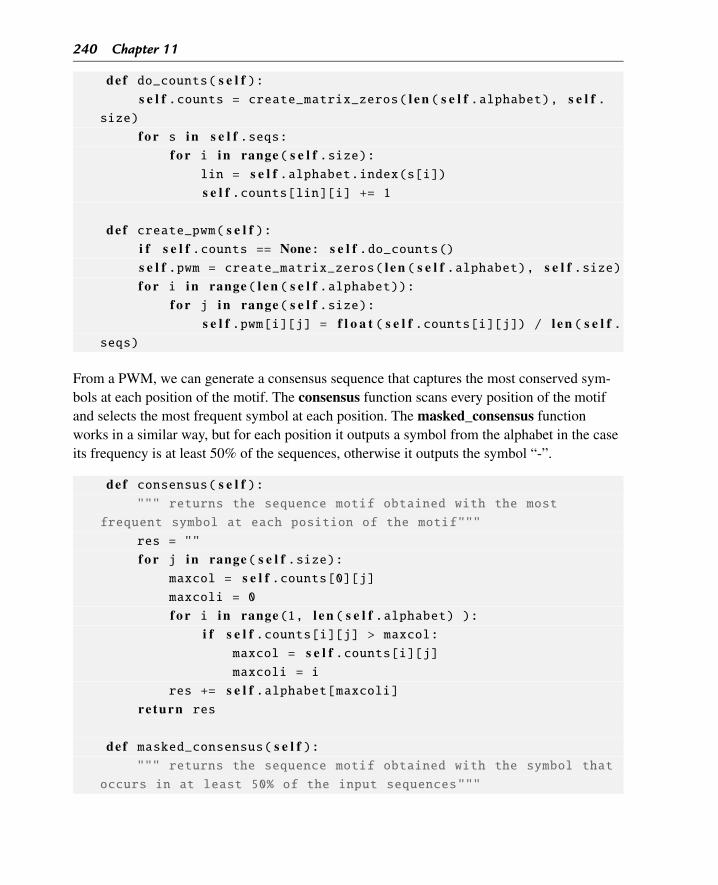
240 Chapter 11

def do_counts( s e l f ):s e l f .counts = create_matrix_zeros( l e n ( s e l f .alphabet), s e l f .

size)

f o r s in s e l f .seqs:f o r i in range( s e l f .size):

lin = s e l f .alphabet.index(s[i])s e l f .counts[lin][i] += 1

def create_pwm( s e l f ):i f s e l f .counts == None: s e l f .do_counts()s e l f .pwm = create_matrix_zeros( l e n ( s e l f .alphabet), s e l f .size)f o r i in range( l e n ( s e l f .alphabet)):

f o r j in range( s e l f .size):s e l f .pwm[i][j] = f l o a t ( s e l f .counts[i][j]) / l e n ( s e l f .

seqs)

From a PWM, we can generate a consensus sequence that captures the most conserved sym-bols at each position of the motif. The consensus function scans every position of the motifand selects the most frequent symbol at each position. The masked_consensus functionworks in a similar way, but for each position it outputs a symbol from the alphabet in the caseits frequency is at least 50% of the sequences, otherwise it outputs the symbol “-”.

def consensus( s e l f ):""" returns the sequence motif obtained with the most

frequent symbol at each position of the motif"""

res = ""

f o r j in range( s e l f .size):maxcol = s e l f .counts[0][j]maxcoli = 0

f o r i in range(1, l e n ( s e l f .alphabet) ):i f s e l f .counts[i][j] > maxcol:

maxcol = s e l f .counts[i][j]maxcoli = i

res += s e l f .alphabet[maxcoli]re turn res

def masked_consensus( s e l f ):""" returns the sequence motif obtained with the symbol that

occurs in at least 50% of the input sequences"""

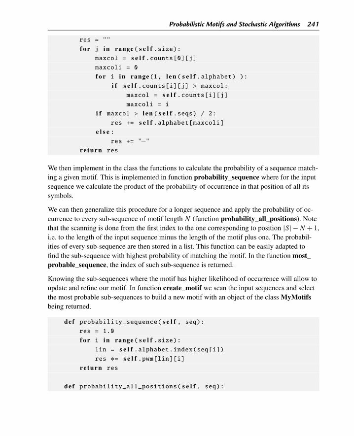
Probabilistic Motifs and Stochastic Algorithms 241

res = ""

f o r j in range( s e l f .size):maxcol = s e l f .counts[0][j]maxcoli = 0

f o r i in range(1, l e n ( s e l f .alphabet) ):i f s e l f .counts[i][j] > maxcol:

maxcol = s e l f .counts[i][j]maxcoli = i

i f maxcol > l e n ( s e l f .seqs) / 2:res += s e l f .alphabet[maxcoli]

e l s e :res += "−"

re turn res

We then implement in the class the functions to calculate the probability of a sequence match-ing a given motif. This is implemented in function probability_sequence where for the inputsequence we calculate the product of the probability of occurrence in that position of all itssymbols.

We can then generalize this procedure for a longer sequence and apply the probability of oc-currence to every sub-sequence of motif length N (function probability_all_positions). Notethat the scanning is done from the first index to the one corresponding to position |S| − N + 1,i.e. to the length of the input sequence minus the length of the motif plus one. The probabil-ities of every sub-sequence are then stored in a list. This function can be easily adapted tofind the sub-sequence with highest probability of matching the motif. In the function most_probable_sequence, the index of such sub-sequence is returned.

Knowing the sub-sequences where the motif has higher likelihood of occurrence will allow toupdate and refine our motif. In function create_motif we scan the input sequences and selectthe most probable sub-sequences to build a new motif with an object of the class MyMotifsbeing returned.

def probability_sequence( s e l f , seq):res = 1.0

f o r i in range( s e l f .size):lin = s e l f .alphabet.index(seq[i])res ∗= s e l f .pwm[lin][i]

re turn res

def probability_all_positions( s e l f , seq):

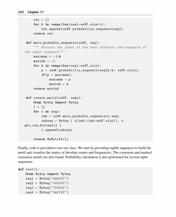
242 Chapter 11

res = []

f o r k in range( l e n (seq)−s e l f .size+1):res.append( s e l f .probability_sequence(seq))

re turn res

def most_probable_sequence( s e l f , seq):""" Returns the index of the most probable sub−sequence of

the input sequence"""

maximum = −1.0maxind = −1f o r k in range( l e n (seq)−s e l f .size):

p = s e l f .probability_sequence(seq[k:k+ s e l f .size])i f (p > maximum):

maximum = p

maxind = k

re turn maxind

def create_motif( s e l f , seqs):from MySeq import MySeql = []

f o r s in seqs:

ind = s e l f .most_probable_sequence(s.seq)subseq = MySeq ( s[ind:(ind+ s e l f .size)], s.

get_seq_biotype() )

l.append(subseq)

re turn MyMotifs(l)

Finally, code is provided to test our class. We start by providing eighth sequences to build themotif and visualize the matrix of absolute counts and frequencies. The consensus and maskedconsensus motifs are also found. Probability calculation is also performed for several inputsequences.

def test():from MySeq import MySeqseq1 = MySeq("AAAGTT")

seq2 = MySeq("CACGTG")

seq3 = MySeq("TTGGGT")

seq4 = MySeq("GACCGT")

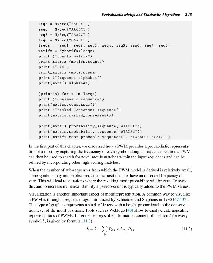
Probabilistic Motifs and Stochastic Algorithms 243

seq5 = MySeq("AACCAT")

seq6 = MySeq("AACCCT")

seq7 = MySeq("AAACCT")

seq8 = MySeq("GAACCT")

lseqs = [seq1, seq2, seq3, seq4, seq5, seq6, seq7, seq8]

motifs = MyMotifs(lseqs)

p r i n t ("Counts matrix")print_matrix (motifs.counts)

p r i n t ("PWM")print_matrix (motifs.pwm)

p r i n t ("Sequence alphabet")p r i n t (motifs.alphabet)

[ p r i n t (s) f o r s in lseqs]

p r i n t ("Consensus sequence")p r i n t (motifs.consensus())p r i n t ("Masked Consensus sequence")p r i n t (motifs.masked_consensus())

p r i n t (motifs.probability_sequence("AAACCT"))p r i n t (motifs.probability_sequence("ATACAG"))p r i n t (motifs.most_probable_sequence("CTATAAACCTTACATC"))

In the first part of this chapter, we discussed how a PWM provides a probabilistic representa-tion of a motif by capturing the frequency of each symbol along its sequence positions. PWMcan then be used to search for novel motifs matches within the input sequences and can berefined by incorporating other high-scoring matches.

When the number of sub-sequences from which the PWM model is derived is relatively small,some symbols may not be observed at some positions, i.e. have an observed frequency ofzero. This will lead to situations where the resulting motif probability will be zero. To avoidthis and to increase numerical stability a pseudo-count is typically added to the PWM values.

Visualization is another important aspect of motif representation. A common way to visualizea PWM is through a sequence logo, introduced by Schneider and Stephens in 1990 [47,137].This type of graphics represents a stack of letters with a height proportional to the conserva-tion level of the motif positions. Tools such as Weblogo [40] allow to easily create appealingrepresentations of PWMs. In sequence logos, the information content of position i for everysymbol b, is given by formula (11.3).

Ii = 2 +∑

b

Pb,i × log2Pb,i (11.3)

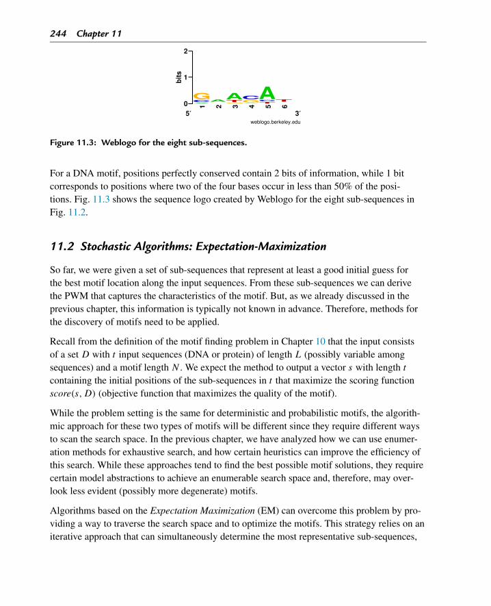
244 Chapter 11

Figure 11.3: Weblogo for the eight sub-sequences.

For a DNA motif, positions perfectly conserved contain 2 bits of information, while 1 bitcorresponds to positions where two of the four bases occur in less than 50% of the posi-tions. Fig. 11.3 shows the sequence logo created by Weblogo for the eight sub-sequences inFig. 11.2.

11.2 Stochastic Algorithms: Expectation-Maximization

So far, we were given a set of sub-sequences that represent at least a good initial guess forthe best motif location along the input sequences. From these sub-sequences we can derivethe PWM that captures the characteristics of the motif. But, as we already discussed in theprevious chapter, this information is typically not known in advance. Therefore, methods forthe discovery of motifs need to be applied.

Recall from the definition of the motif finding problem in Chapter 10 that the input consistsof a set D with t input sequences (DNA or protein) of length L (possibly variable amongsequences) and a motif length N . We expect the method to output a vector s with length t

containing the initial positions of the sub-sequences in t that maximize the scoring functionscore(s,D) (objective function that maximizes the quality of the motif).

While the problem setting is the same for deterministic and probabilistic motifs, the algorith-mic approach for these two types of motifs will be different since they require different waysto scan the search space. In the previous chapter, we have analyzed how we can use enumer-ation methods for exhaustive search, and how certain heuristics can improve the efficiency ofthis search. While these approaches tend to find the best possible motif solutions, they requirecertain model abstractions to achieve an enumerable search space and, therefore, may over-look less evident (possibly more degenerate) motifs.

Algorithms based on the Expectation Maximization (EM) can overcome this problem by pro-viding a way to traverse the search space and to optimize the motifs. This strategy relies on aniterative approach that can simultaneously determine the most representative sub-sequences,

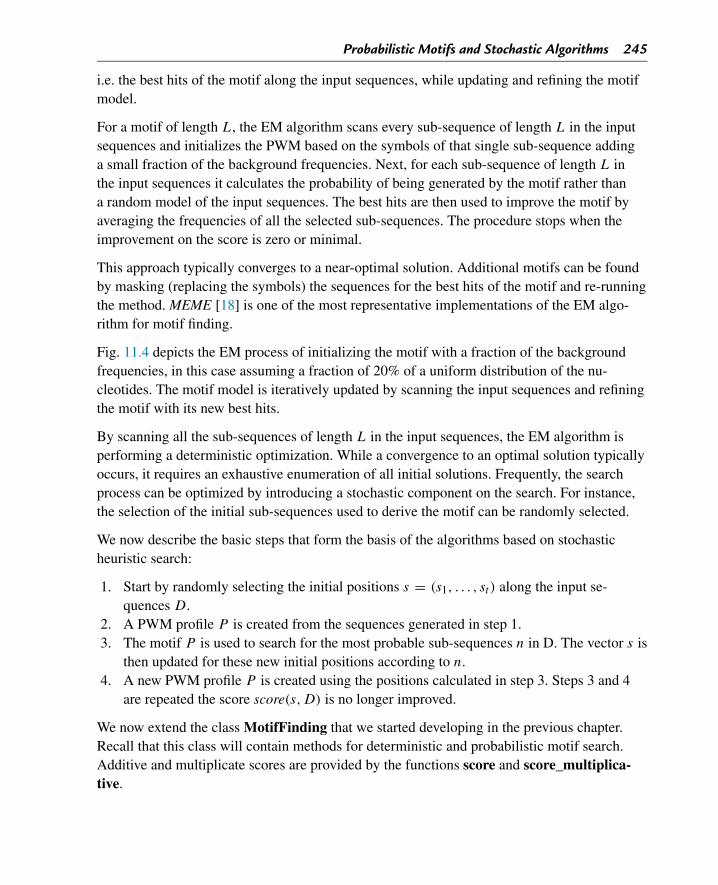
Probabilistic Motifs and Stochastic Algorithms 245

i.e. the best hits of the motif along the input sequences, while updating and refining the motifmodel.

For a motif of length L, the EM algorithm scans every sub-sequence of length L in the inputsequences and initializes the PWM based on the symbols of that single sub-sequence addinga small fraction of the background frequencies. Next, for each sub-sequence of length L inthe input sequences it calculates the probability of being generated by the motif rather thana random model of the input sequences. The best hits are then used to improve the motif byaveraging the frequencies of all the selected sub-sequences. The procedure stops when theimprovement on the score is zero or minimal.

This approach typically converges to a near-optimal solution. Additional motifs can be foundby masking (replacing the symbols) the sequences for the best hits of the motif and re-runningthe method. MEME [18] is one of the most representative implementations of the EM algo-rithm for motif finding.

Fig. 11.4 depicts the EM process of initializing the motif with a fraction of the backgroundfrequencies, in this case assuming a fraction of 20% of a uniform distribution of the nu-cleotides. The motif model is iteratively updated by scanning the input sequences and refiningthe motif with its new best hits.

By scanning all the sub-sequences of length L in the input sequences, the EM algorithm isperforming a deterministic optimization. While a convergence to an optimal solution typicallyoccurs, it requires an exhaustive enumeration of all initial solutions. Frequently, the searchprocess can be optimized by introducing a stochastic component on the search. For instance,the selection of the initial sub-sequences used to derive the motif can be randomly selected.

We now describe the basic steps that form the basis of the algorithms based on stochasticheuristic search:

1. Start by randomly selecting the initial positions s = (s1, . . . , st ) along the input se-quences D.

2. A PWM profile P is created from the sequences generated in step 1.3. The motif P is used to search for the most probable sub-sequences n in D. The vector s is

then updated for these new initial positions according to n.4. A new PWM profile P is created using the positions calculated in step 3. Steps 3 and 4

are repeated the score score(s,D) is no longer improved.

We now extend the class MotifFinding that we started developing in the previous chapter.Recall that this class will contain methods for deterministic and probabilistic motif search.Additive and multiplicate scores are provided by the functions score and score_multiplica-tive.

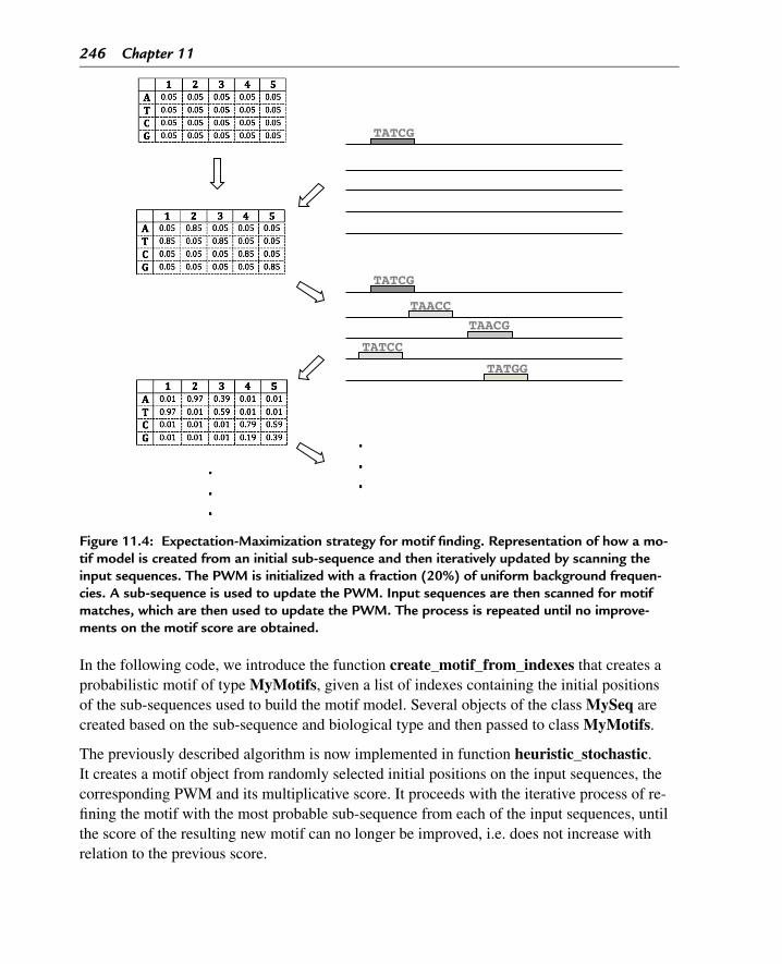
246 Chapter 11

Figure 11.4: Expectation-Maximization strategy for motif finding. Representation of how a mo-tif model is created from an initial sub-sequence and then iteratively updated by scanning theinput sequences. The PWM is initialized with a fraction (20%) of uniform background frequen-cies. A sub-sequence is used to update the PWM. Input sequences are then scanned for motifmatches, which are then used to update the PWM. The process is repeated until no improve-ments on the motif score are obtained.

In the following code, we introduce the function create_motif_from_indexes that creates aprobabilistic motif of type MyMotifs, given a list of indexes containing the initial positionsof the sub-sequences used to build the motif model. Several objects of the class MySeq arecreated based on the sub-sequence and biological type and then passed to class MyMotifs.

The previously described algorithm is now implemented in function heuristic_stochastic.It creates a motif object from randomly selected initial positions on the input sequences, thecorresponding PWM and its multiplicative score. It proceeds with the iterative process of re-fining the motif with the most probable sub-sequence from each of the input sequences, untilthe score of the resulting new motif can no longer be improved, i.e. does not increase withrelation to the previous score.

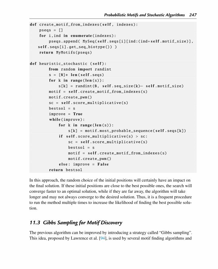
Probabilistic Motifs and Stochastic Algorithms 247

def create_motif_from_indexes( s e l f , indexes):pseqs = []

f o r i,ind in enumerate(indexes):pseqs.append( MySeq( s e l f .seqs[i][ind:(ind+ s e l f .motif_size)],

s e l f .seqs[i].get_seq_biotype()) )re turn MyMotifs(pseqs)

def heuristic_stochastic ( s e l f ):from random import randints = [0]∗ l e n ( s e l f .seqs)f o r k in range( l e n (s)):

s[k] = randint(0, s e l f .seq_size(k)− s e l f .motif_size)motif = s e l f .create_motif_from_indexes(s)motif.create_pwm()

sc = s e l f .score_multiplicative(s)bestsol = s

improve = Truewhi l e(improve):

f o r k in range( l e n (s)):s[k] = motif.most_probable_sequence( s e l f .seqs[k])

i f s e l f .score_multiplicative(s) > sc:sc = s e l f .score_multiplicative(s)bestsol = s

motif = s e l f .create_motif_from_indexes(s)motif.create_pwm()

e l s e : improve = F a l s ere turn bestsol

In this approach, the random choice of the initial positions will certainly have an impact onthe final solution. If these initial positions are close to the best possible ones, the search willconverge faster to an optimal solution, while if they are far away, the algorithm will takelonger and may not always converge to the desired solution. Thus, it is a frequent procedureto run the method multiple times to increase the likelihood of finding the best possible solu-tion.

11.3 Gibbs Sampling for Motif Discovery

The previous algorithm can be improved by introducing a strategy called “Gibbs sampling”.This idea, proposed by Lawrence et al. [94], is used by several motif finding algorithms and

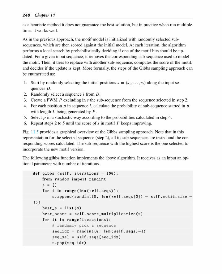
248 Chapter 11

as a heuristic method it does not guarantee the best solution, but in practice when run multipletimes it works well.

As in the previous approach, the motif model is initialized with randomly selected sub-sequences, which are then scored against the initial model. At each iteration, the algorithmperforms a local search by probabilistically deciding if one of the motif hits should be up-dated. For a given input sequence, it removes the corresponding sub-sequence used to modelthe motif. Then, it tries to replace with another sub-sequence, computes the score of the motif,and decides if the update is kept. More formally, the steps of the Gibbs sampling approach canbe enumerated as:

1. Start by randomly selecting the initial positions s = (s1, . . . , st ) along the input se-quences D.

2. Randomly select a sequence i from D.3. Create a PWM P excluding in s the sub-sequence from the sequence selected in step 2.4. For each position p in sequence i, calculate the probability of sub-sequence started in p

with length L being generated by P .5. Select p in a stochastic way according to the probabilities calculated in step 4.6. Repeat steps 2 to 5 until the score of s in motif P keeps improving.

Fig. 11.5 provides a graphical overview of the Gibbs sampling approach. Note that in thisrepresentation for the selected sequence (step 2), all its sub-sequences are tested and the cor-responding scores calculated. The sub-sequence with the highest score is the one selected toincorporate the new motif version.

The following gibbs function implements the above algorithm. It receives as an input an op-tional parameter with number of iterations.

def gibbs ( s e l f , iterations = 100):from random import randints = []

f o r i in range( l e n ( s e l f .seqs)):s.append(randint(0, l e n ( s e l f .seqs[0]) − s e l f .motif_size −

1))

best_s = l i s t (s)best_score = s e l f .score_multiplicative(s)f o r it in range(iterations):

# randomly pick a sequence

seq_idx = randint(0, l e n ( s e l f .seqs)−1)seq_sel = s e l f .seqs[seq_idx]s.pop(seq_idx)

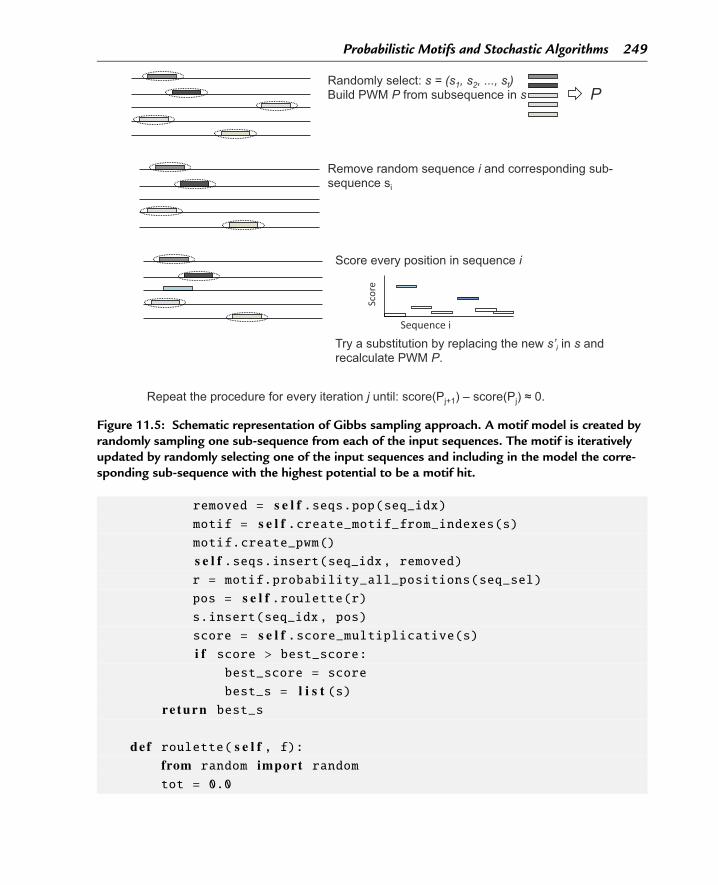
Probabilistic Motifs and Stochastic Algorithms 249

Figure 11.5: Schematic representation of Gibbs sampling approach. A motif model is created byrandomly sampling one sub-sequence from each of the input sequences. The motif is iterativelyupdated by randomly selecting one of the input sequences and including in the model the corre-sponding sub-sequence with the highest potential to be a motif hit.

removed = s e l f .seqs.pop(seq_idx)motif = s e l f .create_motif_from_indexes(s)motif.create_pwm()

s e l f .seqs.insert(seq_idx, removed)r = motif.probability_all_positions(seq_sel)

pos = s e l f .roulette(r)s.insert(seq_idx, pos)

score = s e l f .score_multiplicative(s)i f score > best_score:

best_score = score

best_s = l i s t (s)re turn best_s

def roulette( s e l f , f):from random import randomtot = 0.0

250 Chapter 11

f o r x in f: tot += (0.01 + x)

val = random() ∗ totacum = 0.0

idx = 0

whi le acum < val:acum += (f[idx] + 0.01)

idx += 1

re turn idx−1After determining the probabilities of all the sub-sequences along the removed sequence, onecould determine the new best position as the one with the highest score with relation to themotif. Instead, a different strategy is used. With the roulette function a sample space for theexperiment of spinning once a roulette wheel is created. All positions have a chance of beingpicked, but this chance is proportional to their score.

We can now compare the results obtained with a general stochastic algorithm and those fromGibbs sampling.

def test_heuristic_algorithms():mf = MotifFinding()

mf.read_file("exampleMotifs.txt","dna")

p r i n t ("Heuristic stochastic")sol = mf.heuristic_stochastic()

p r i n t ("Solution: ", sol)p r i n t ("Score:", mf.score(sol))p r i n t ("Score mult:", mf.score_multiplicative(sol))p r i n t ("Consensus:", mf.create_motif_from_indexes(sol).consensus())

sol2 = mf.gibbs(1000)

p r i n t ("Score:", mf.score(sol2))p r i n t ("Score mult:", mf.score_multiplicative(sol2))p r i n t ("Consensus:", mf.create_motif_from_indexes(sol2).consensus())

11.4 Probabilistic Motifs in BioPython

The package Bio.Motifs of BioPython provides a set of functionalities to work with proba-bilistic motifs, their representation and search over target sequences. We will show here a fewexamples, while a more complete coverage can be found in Chapter 14 of the tutorial.

Probabilistic Motifs and Stochastic Algorithms 251

The following code example shows how to create an object of the class Motif, which repre-sents a motif in BioPython, from a set of instances (sequences represented as a list of objectsof class Seq). The content of the motif m is then printed, including its consensus, the rawcounts of each symbol for each position, the PWM, and the created PSSM. The last line willsave a logo of the motif to your current folder.

from Bio.Seq import Seqfrom Bio import motifsfrom Bio.Alphabet import IUPAC

instances = []

instances.append(Seq("TATAA",IUPAC.unambiguous_dna))

instances.append(Seq("TATTA",IUPAC.unambiguous_dna))

instances.append(Seq("TTTAT",IUPAC.unambiguous_dna))

instances.append(Seq("TATAC",IUPAC.unambiguous_dna))

m = motifs.create(instances, IUPAC.unambiguous_dna)

p r i n t (m)p r i n t ( l e n (m))p r i n t (m.consensus)p r i n t (m.counts)p r i n t (m.pwm)p r i n t (m.pssm)

m.weblogo("mymotif.png")

Notice in the results of the previous script that the PSSM has a few positions filled with“-inf”, representing minus infinity. This happens due to the presence of zeros in the PWM.One way to prevent this situation is the use of pseudo-counts, as discussed above. The follow-ing code shows how to add pseudo-counts in the example, re-generating the respective PWMand PSSM.

pwm = m.counts.normalize(pseudocounts=0.5)

pssm = pwm.log_odds()

p r i n t (pwm)p r i n t (pssm)

It is important to mention that there are also functions that allow to read motifs in differ-ent formats, with the functions motifs.read or motifs.parse (for multiple instances from

252 Chapter 11

the same file). These allow to load motifs from databases and tools as JASPAR, MEME, orTRANSFAC. Also, the function motifs.write allows to write motifs in a selected format.

Another important functionality of this module is the ability to search for motif occurrencesin target sequences. One possible type of search is to find exact occurrences of the instancesused to create the motif. This is done in the next example for a toy sequence to exemplify itsuse.

test_seq=Seq("TTTTATACACTGCATATAACAACCCAAGCATTATAA", IUPAC.

unambiguous_dna)

f o r pos, seq in m.instances.search(test_seq):

p r i n t (pos, " ", seq)

Probably a more useful feature is the ability to look for matches of the motif using the PSSMto score those matches and defining proper thresholds for acceptance. This is done in the ex-ample below defining as the minimum threshold a score of 4 to accept the match.

f o r position, score in pssm.search(test_seq, threshold=4.0):

p r i n t ("Position %d: score = %5.3f" % (position, score) )

Notice that in the result some positions are returned as negative numbers. These are matchesof the motif in the reverse complement of the original sequence, which is also scanned.

Finally, we will show how we can provide the scores for all possible positions of the motif inthe sequence in a list by using the function calculate.

p r i n t (pssm.calculate(test_seq))

The support of BioPython for motif discovery is quite limited, mainly consisting on the abilityto parse the results of the MEME tool, using the input/output functions mentioned above.

Bibliographic Notes and Further Reading

There is an extensive research on motif finding with many algorithms proposed over the lastdecades. This prompts the question of which of the methods and algorithms are better for thetask. The answer to this question depends on many aspects including the characteristics ofthe input data and the defined constraints on the search process. In order to provide a moregeneric view on the performance of different methods several small and large-scale compar-isons have been done. We refer to the work of Tompa et al. [148] that provides a comparisonof thirteen methods for the identification of transcription factor binding sites.

Probabilistic Motifs and Stochastic Algorithms 253

Beyond sequence conservation, there are other features that may indicate that a motif rep-resents a true biological signal. This includes among other aspects location specificity thatcaptures the bias on motif localization. Example of this includes motifs that occur prefer-entially on the promoter region close to the transcription start site. Motif co-occurrence isanother interesting aspect, where motifs may occur in modules in combination with othermotifs. Several algorithms take advantage of one or more of these features to determine therelevance of the discovered motifs and discard spurious discoveries [153].

Here, we quantified the interest of a motif based on its probability or respective score. Nev-ertheless, other measures were developed to quantify the interest of a motif and can be usedas complementary measures. For instance, measures like information gain, surprise, mutualinformation capture how unexpected is the motif occurrence given the background compo-sition of the input sequences. We refer to the work of Li and Tompa [101] and Ferreira andAzevedo [65] which have focused on the evaluation of different measures of motif interest.

Exercises and Programming Projects

Exercises

1. Within the class MyMotifs create a function that receives as input a constant and addsthis constant as a pseudo-count of the PWM.

2. Write a function for the class MyMotifs that given an input sequence and a score thresh-old, reports all the motif matches with a score higher than a given threshold.

3. In the Expectation-Maximization algorithm, the PWM is initialized with a fraction of thebackground frequencies. Write a function that given a fraction ((0,1]) and the set of inputsequences, initializes the PWM accordingly.

Programming Projects

1. Add to the class MyMotifs the possibility of calculating PSSM and using those to scorehits of the motif in sequences. Consider using pseudo-counts to avoid problems with thelogarithm of zero. Implement search of motifs over sequences ranking the results andfiltering through the use of a minimum score threshold. Consider the option to searchfor motifs not only in the sequence, but also in the reverse complement (assuming DNAsequences).

2. Implement a function to generate a random solution for a motif finding problem. Basedon this function, implement a random search algorithm, that generates N solutions usingthe previous function, and selects the one with highest score (N is a parameter). Comparethe results of this algorithm with the ones developed in this chapter, providing the samemaximum number of solutions to each.

CHAPTER 12

Hidden Markov ModelsIn this chapter we present Hidden Markov Models (HMMs), as stochastic models that cap-ture statistical regularities from the input sequences and allow to devise algorithms for motiffinding and database search. We will discuss the elements that compose an HMM and howinput sequences can be evaluated in terms of their likelihood. How to improve the HMMsparameters from additional training sequences will also be discussed. Implementations forsimplified versions of the main algorithms in Python are provided. Finally, examples of someof the many applications of HMM in biological sequence analysis are provided.

12.1 Introduction: What Are Hidden Markov Models?

In Chapter 5, we have seen that the string matching problem consists of finding in a se-quence S, defined over an alphabet �, all the occurrences of pattern P (defined in the samealphabet). In Section 5.4, we introduced the Deterministic Finite Automaton (DFA), an ab-stract mathematical concept, that can be used to represent a string language, i.e. the set ofstrings that match a given pattern. The basic idea is to build an automaton from the pattern.Then, once the DFA is built multiple strings can be scanned to look for the match of the pat-tern. The DFA is represented as a graph with a finite number of states. Each symbol in thepattern corresponds to a state and every matched symbol sends the automaton to a new state.The DFA has a start and an end state. If the end state is reached, it means that the scannedstring is accepted. Using a DFA, only one pass over the input string is required, making it avery efficient method for string matching. DFAs provide a deterministic pattern search, i.e.either match or not the scanned sequence, as it happened also with regular expressions.

However, in biological sequence analysis, the events associated to a sequence are often proba-bilistic. Examples of this include for instance, the classification of the subcellular localization(e.g. cytosol, nucleus or the membrane) of a protein given its sequence; the presence of pro-tein domains within a sequence or the binding probability of a transcription factor on thesequence of a gene promoter region.

Hidden Markov Models (HMMs) are probabilistic models that capture statistical regulari-ties within a linear sequence. As we will see, HMMs are very well suited for the mentionedtasks. Indeed, HMMs have been largely used in many different problems in molecular biol-ogy, including gene finding, profile searches, multiple sequence alignment, identification ofregulatory sites, or the prediction of secondary structure in proteins.

Bioinformatics Algorithms. DOI: 10.1016/B978-0-12-812520-5.00012-2Copyright © 2018 Elsevier Inc. All rights reserved. 255

256 Chapter 12

Let us now examine the structure of an HMM by looking at a specific example. Consider theelements of a mature mRNA. It contains a tripartite structure that starts with a 5’ untranslatedregion (5’ UTR), a region that will be translated and code for a protein (CDS) and ends witha 3’ untranslated region (3’UTR) [112]. Moreover, we also know that the CDS region shouldstart with a start codon (ATG) and end with one of the three stop codons. Here, for sake ofsimplicity we will omit the codon details.

So, in this case, we have a grammatical structure that defines a mature mRNA. We can viewthe untranslated and CDS regions as words. The sentences of our grammar will have certainrules, like the fact that the 5’UTR should always precede the CDS and the 3’UTR should al-ways come after the CDS. We can also assume that the three elements will always be presentin a mature mRNA. Our goal will be to scan a sequence and label each of its nucleotide sym-bols with the corresponding region. A probability will be associated at every labeling point.The representation of each region or label will be called state of the HMM.

When scanning a symbol at a given state, there is a certain probability that the next symbolwill belong to the current state or not. The probabilities associated with a change of stateare called transition probabilities and depend on several factors including, for instance, thetypical sequence length of the corresponding region. In this case, let’s consider that, whenscanning a symbol on the 5’UTR, we have 0.8 probability that the next symbol will also bepart of the 5’UTR and 0.2 probability that it will change to the CDS region. We can ascertainprobabilities to the other regions in a similar manner. To model our HMM we will need threestates, plus two additional states that define the start and the end of the sequence. The startstate represents the probability of starting in any of the defined states.

It is well known that the composition of mRNA regions differ depending on the species [159].Considering, for instance, that the G + C content in the 5’UTR is of 60%, in the CDS of 50%and in the 3’UTR of 30%, these compositional frequencies will determine the emission proba-bilities that provide the probability of symbol being emitted by a state.

To determine the probability of a sequence, we just need to multiply the probability of thesymbol in the respective state and the respective transition probability. Consider for instancethe string TAGTTA with 3 nucleotides within the CDS and 3 nucleotides in the 3’UTR. Theprobability of this sequence will be given by:

PCDS(T ) × P(CDS|CDS) × PCDS(A) × P(CDS|CDS) × PCDS(G)

×P(CDS|3U) × P3U(T ) × P(3U |3U) × P3U(T ) × P(3U |3U) × P3U(A)

= 0.25 × 0.9 × 0.25 × 0.9 × 0.25 × 0.1 × 0.35 × 0.8 × 0.35 × 0.8 × 0.35

= 3.47287 × 10−5

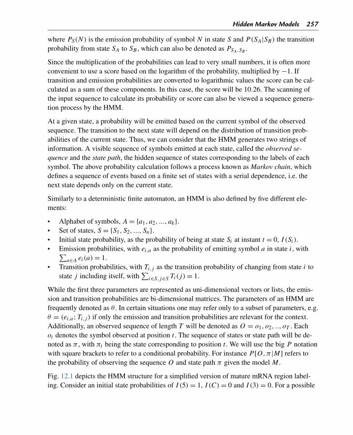
Hidden Markov Models 257

where PS(N) is the emission probability of symbol N in state S and P(SA|SB) the transitionprobability from state SA to SB , which can also be denoted as PSA,SB

.

Since the multiplication of the probabilities can lead to very small numbers, it is often moreconvenient to use a score based on the logarithm of the probability, multiplied by −1. Iftransition and emission probabilities are converted to logarithmic values the score can be cal-culated as a sum of these components. In this case, the score will be 10.26. The scanning ofthe input sequence to calculate its probability or score can also be viewed a sequence genera-tion process by the HMM.

At a given state, a probability will be emitted based on the current symbol of the observedsequence. The transition to the next state will depend on the distribution of transition prob-abilities of the current state. Thus, we can consider that the HMM generates two strings ofinformation. A visible sequence of symbols emitted at each state, called the observed se-quence and the state path, the hidden sequence of states corresponding to the labels of eachsymbol. The above probability calculation follows a process known as Markov chain, whichdefines a sequence of events based on a finite set of states with a serial dependence, i.e. thenext state depends only on the current state.

Similarly to a deterministic finite automaton, an HMM is also defined by five different ele-ments:

• Alphabet of symbols, A = {a1, a2, ..., ak}.• Set of states, S = {S1, S2, ..., Sn}.• Initial state probability, as the probability of being at state Si at instant t = 0, I (Si).• Emission probabilities, with ei,a as the probability of emitting symbol a in state i, with∑

a∈A ei(a) = 1.• Transition probabilities, with Ti,j as the transition probability of changing from state i to

state j including itself, with∑

i∈S,j∈S Ti(j) = 1.

While the first three parameters are represented as uni-dimensional vectors or lists, the emis-sion and transition probabilities are bi-dimensional matrices. The parameters of an HMM arefrequently denoted as θ . In certain situations one may refer only to a subset of parameters, e.g.θ = (ei,a;Ti,j ) if only the emission and transition probabilities are relevant for the context.Additionally, an observed sequence of length T will be denoted as O = o1, o2, .., oT . Eachot denotes the symbol observed at position t . The sequence of states or state path will be de-noted as π , with πt being the state corresponding to position t . We will use the big P notationwith square brackets to refer to a conditional probability. For instance P [O,π |M] refers tothe probability of observing the sequence O and state path π given the model M .

Fig. 12.1 depicts the HMM structure for a simplified version of mature mRNA region label-ing. Consider an initial state probabilities of I (5) = 1, I (C) = 0 and I (3) = 0. For a possible

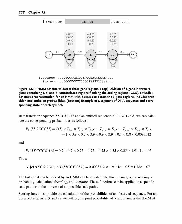
258 Chapter 12

Figure 12.1: HMM scheme to detect three gene regions. (Top) Division of a gene in three re-gions containing a 5’ and 3’ untranslated regions flanking the coding regions (CDS). (Middle)Schematic representation for an HMM with 5 states to detect the 3 gene regions. Includes tran-sition and emission probabilities. (Bottom) Example of a segment of DNA sequence and corre-sponding state of each symbol.

state transition sequence 55CCCC33 and an emitted sequence AT CGCGAA, we can calcu-late the corresponding probabilities as follows:

PT [55CCCC33] = I (5) × T5,5 × T5,C × TC,C × TC,C × TC,C × TC,C × TC,3 × T3,3

= 1 × 0.8 × 0.2 × 0.9 × 0.9 × 0.9 × 0.1 × 0.8 ≈ 0.0093312

and

Pe [AT CGCGAA] = 0.2 × 0.2 × 0.25 × 0.25 × 0.25 × 0.35 × 0.35 ≈ 1.9141e − 05

Thus:

P [e(AT CGCGC) ∧ T (55CCCC33)] = 0.0093312 × 1.9141e − 05 ≈ 1.78e − 07

The tasks that can be solved by an HMM can be divided into three main groups: scoring orprobability calculation, decoding, and learning. These functions can be applied to a specificstate path or to the universe of all possible state paths.

Scoring functions provide the calculation of the probabilities of an observed sequence. For anobserved sequence O and a state path π , the joint probability of S and π under the HMM M

Hidden Markov Models 259

is P [O,π |M]. This can be calculated as in the example above where we obtain the joint prod-uct of emission and transition probabilities. If no state path is provided, the goal is to calculatethe total probability of the sequence, P(O|M). This probability can be yield by summing theprobabilities of all possible paths, which is an exponentially large number of paths, but can beefficiently calculated with the Forward algorithm. This algorithm provides the probability thatthe HMM M will output a sequence o1...ot and reach the state Si at position t . The Forwardprobability is denoted as αt(Si) and equivalently as P [O = o1...ot , πt = Si |M].Another important calculation is to determine the backward probability. This provides theprobability of starting at state Si and position t and generating the remainder of the observedsequence ot ...oT . The Backward probability is denoted as βt(Si) and equivalently as P [O =ot ...oT |πt = Si |M].Decoding refers to the process of determining the most likely underlying sequence of statesgiven an observed sequence. In our previous example this refers to the task of determiningthe sequence of states 5U, CDS, or 3U for each of the observed sequence symbol. Given anHMM M and an observed sequence O , the task of the decoder is to find the most probablestate path π . Here, we will apply a dynamic programming algorithm, called Viterbi algorithm,to find the path with the maximum score over all paths. A trace-back function can be used tokeep track of all visited paths and to determine the most probable path.

Another relevant question is to determine the total probability of the symbol ot to be emittedby the state k, when considering all state paths. This is called posterior probability and de-noted as P [πt = k|O,M]. This probability is given by the product of the forward probabilityαt(k) and the backward probability βt (k) divided by the probability of O , P(O).

In our mRNA HMM example we have defined a priori the parameters of the model, whichwe could have determined either using previous knowledge or estimating from observed data.If during the analysis process we acquire more data we may want to adjust these parametersand optimize our model. By analyzing a given dataset we can also learn these parameters. Ourgoal is to find the parameters θ = (ei,a;Ti,j ) that maximize the probability of the observedsequence under the model M, P(O|M). If the observed sequence has been labeled, i.e. thestate path is known, then a supervised learning is performed. In this case, the emission andtransition probabilities are directly inferred from the training data. If the training sequencesare unlabeled, then unsupervised learning is performed.

Here, an Expectation-Maximization algorithm called Baum-Welch will be used for learning.Briefly, the algorithm starts with best guess for the parameters θ of the model M . It then esti-mates the emission and transition probabilities from the data. It updates the model accordingto these new values. It iterates on this procedure until the parameters θ of the model M con-verge.

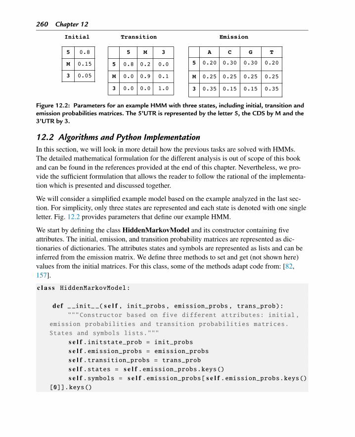
260 Chapter 12

Figure 12.2: Parameters for an example HMM with three states, including initial, transition andemission probabilities matrices. The 5’UTR is represented by the letter 5, the CDS by M and the3’UTR by 3.

12.2 Algorithms and Python ImplementationIn this section, we will look in more detail how the previous tasks are solved with HMMs.The detailed mathematical formulation for the different analysis is out of scope of this bookand can be found in the references provided at the end of this chapter. Nevertheless, we pro-vide the sufficient formulation that allows the reader to follow the rational of the implementa-tion which is presented and discussed together.

We will consider a simplified example model based on the example analyzed in the last sec-tion. For simplicity, only three states are represented and each state is denoted with one singleletter. Fig. 12.2 provides parameters that define our example HMM.

We start by defining the class HiddenMarkovModel and its constructor containing fiveattributes. The initial, emission, and transition probability matrices are represented as dic-tionaries of dictionaries. The attributes states and symbols are represented as lists and can beinferred from the emission matrix. We define three methods to set and get (not shown here)values from the initial matrices. For this class, some of the methods adapt code from: [82,157].

c l a s s HiddenMarkovModel:

def _ _init_ _( s e l f , init_probs, emission_probs , trans_prob):"""Constructor based on five different attributes: initial,

emission probabilities and transition probabilities matrices.

States and symbols lists."""

s e l f .initstate_prob = init_probss e l f .emission_probs = emission_probss e l f .transition_probs = trans_probs e l f .states = s e l f .emission_probs.keys()s e l f .symbols = s e l f .emission_probs[ s e l f .emission_probs.keys()

[0]].keys()

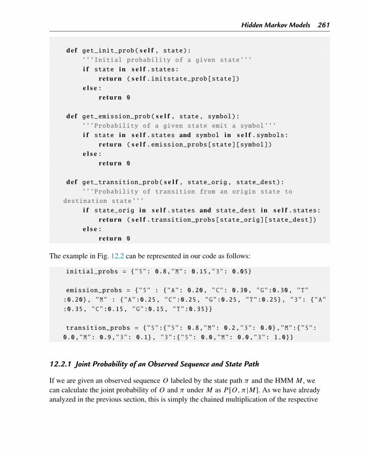
Hidden Markov Models 261

def get_init_prob( s e l f , state):’’’Initial probability of a given state’’’

i f state in s e l f .states:re turn ( s e l f .initstate_prob[state])

e l s e :re turn 0

def get_emission_prob( s e l f , state, symbol):’’’Probability of a given state emit a symbol’’’

i f state in s e l f .states and symbol in s e l f .symbols:re turn ( s e l f .emission_probs[state][symbol])

e l s e :re turn 0

def get_transition_prob( s e l f , state_orig, state_dest):’’’Probability of transition from an origin state to

destination state’’’

i f state_orig in s e l f .states and state_dest in s e l f .states:re turn ( s e l f .transition_probs[state_orig][state_dest])

e l s e :re turn 0

The example in Fig. 12.2 can be represented in our code as follows:

initial_probs = {"5": 0.8,"M": 0.15,"3": 0.05}

emission_probs = {"5" : {"A": 0.20, "C": 0.30, "G":0.30, "T"

:0.20}, "M" : {"A":0.25, "C":0.25, "G":0.25, "T":0.25}, "3": {"A"

:0.35, "C":0.15, "G":0.15, "T":0.35}}

transition_probs = {"5":{"5": 0.8,"M": 0.2,"3": 0.0},"M":{"5":

0.0,"M": 0.9,"3": 0.1}, "3":{"5": 0.0,"M": 0.0,"3": 1.0}}

12.2.1 Joint Probability of an Observed Sequence and State Path

If we are given an observed sequence O labeled by the state path π and the HMM M , wecan calculate the joint probability of O and π under M as P [O,π |M]. As we have alreadyanalyzed in the previous section, this is simply the chained multiplication of the respective

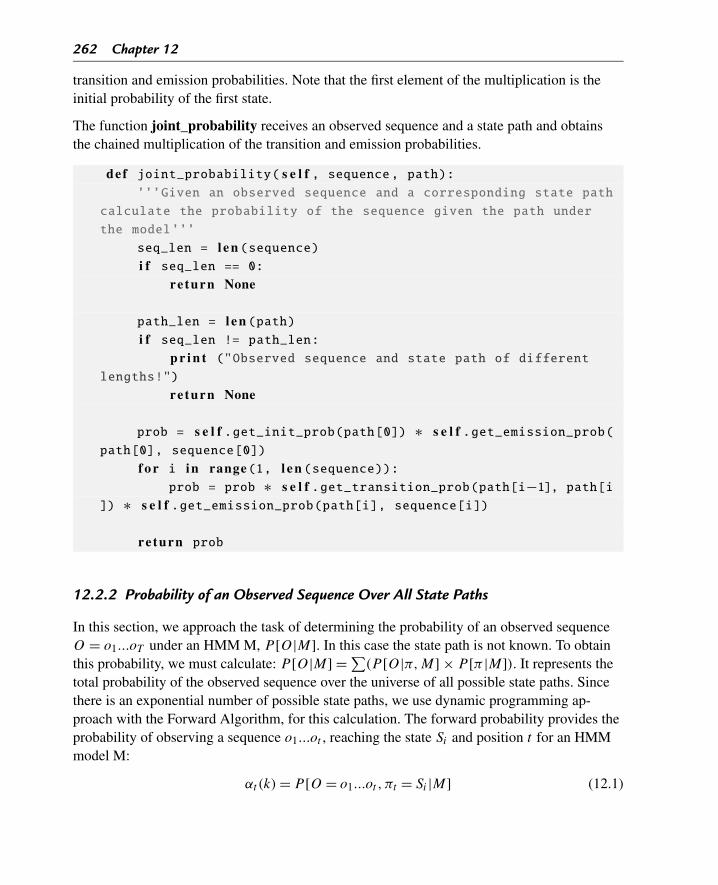
262 Chapter 12

transition and emission probabilities. Note that the first element of the multiplication is theinitial probability of the first state.

The function joint_probability receives an observed sequence and a state path and obtainsthe chained multiplication of the transition and emission probabilities.

def joint_probability( s e l f , sequence, path):’’’Given an observed sequence and a corresponding state path

calculate the probability of the sequence given the path under

the model’’’

seq_len = l e n (sequence)i f seq_len == 0:

re turn None

path_len = l e n (path)i f seq_len != path_len:

p r i n t ("Observed sequence and state path of differentlengths!")

re turn None

prob = s e l f .get_init_prob(path[0]) ∗ s e l f .get_emission_prob(path[0], sequence[0])

f o r i in range(1, l e n (sequence)):prob = prob ∗ s e l f .get_transition_prob(path[i−1], path[i

]) ∗ s e l f .get_emission_prob(path[i], sequence[i])

re turn prob

12.2.2 Probability of an Observed Sequence Over All State Paths

In this section, we approach the task of determining the probability of an observed sequenceO = o1...oT under an HMM M, P [O|M]. In this case the state path is not known. To obtainthis probability, we must calculate: P [O|M] = ∑

(P [O|π,M] × P [π |M]). It represents thetotal probability of the observed sequence over the universe of all possible state paths. Sincethere is an exponential number of possible state paths, we use dynamic programming ap-proach with the Forward Algorithm, for this calculation. The forward probability provides theprobability of observing a sequence o1...ot , reaching the state Si and position t for an HMMmodel M:

αt(k) = P [O = o1...ot , πt = Si |M] (12.1)

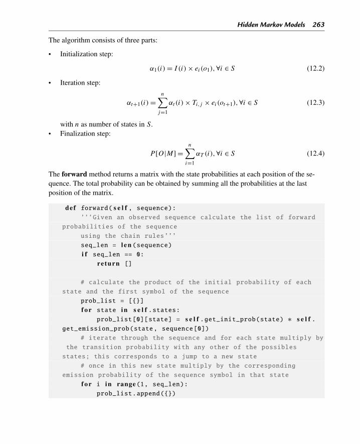
Hidden Markov Models 263

The algorithm consists of three parts:

• Initialization step:

α1(i) = I (i) × ei(o1),∀i ∈ S (12.2)

• Iteration step:

αt+1(i) =n∑

j=1

αt(i) × Ti,j × ei(ot+1),∀i ∈ S (12.3)

with n as number of states in S.• Finalization step:

P [O|M] =n∑

i=1

αT (i),∀i ∈ S (12.4)

The forward method returns a matrix with the state probabilities at each position of the se-quence. The total probability can be obtained by summing all the probabilities at the lastposition of the matrix.

def forward( s e l f , sequence):’’’Given an observed sequence calculate the list of forward

probabilities of the sequence

using the chain rules’’’

seq_len = l e n (sequence)i f seq_len == 0:

re turn []

# calculate the product of the initial probability of each

state and the first symbol of the sequence

prob_list = [{}]

f o r state in s e l f .states:prob_list[0][state] = s e l f .get_init_prob(state) ∗ s e l f .

get_emission_prob(state, sequence[0])

# iterate through the sequence and for each state multiply by

the transition probability with any other of the possibles

states; this corresponds to a jump to a new state

# once in this new state multiply by the corresponding

emission probability of the sequence symbol in that state

f o r i in range(1, seq_len):prob_list.append({})

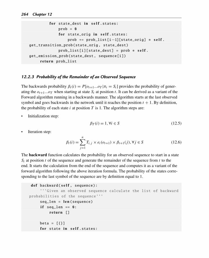
264 Chapter 12

f o r state_dest in s e l f .states:prob = 0

f o r state_orig in s e l f .states:prob += prob_list[i−1][state_orig] ∗ s e l f .

get_transition_prob(state_orig, state_dest)

prob_list[i][state_dest] = prob ∗ s e l f .get_emission_prob(state_dest, sequence[i])

re turn prob_list

12.2.3 Probability of the Remainder of an Observed Sequence

The backwards probability βt (i) = P [ot+1...oT |πt = Si] provides the probability of gener-ating the ot+1...oT when starting at state Si at position t . It can be derived as a variant of theForward algorithm running in a backwards manner. The algorithm starts at the last observedsymbol and goes backwards in the network until it reaches the position t + 1. By definition,the probability of each state i at position T is 1. The algorithm steps are:

• Initialization step:

βT (i) = 1,∀i ∈ S (12.5)

• Iteration step:

βt(i) =n∑

j=1

Ti,j × ei(ot+1) × βt+1(j),∀j ∈ S (12.6)

The backward function calculates the probability for an observed sequence to start in a stateSi at position t of the sequence and generate the remainder of the sequence from t to theend. It starts the calculation from the end of the sequence and computes it as a variant of theforward algorithm following the above iteration formula. The probability of the states corre-sponding to the last symbol of the sequence are by definition equal to 1.

def backward( s e l f , sequence):’’’Given an observed sequence calculate the list of backward

probabilities of the sequence’’’

seq_len = l e n (sequence)i f seq_len == 0:

re turn []

beta = [{}]

f o r state in s e l f .states:

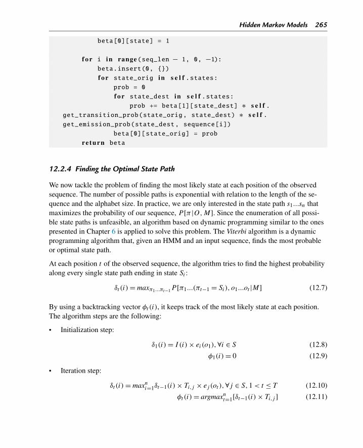
Hidden Markov Models 265

beta[0][state] = 1

f o r i in range(seq_len − 1, 0, −1):beta.insert(0, {})

f o r state_orig in s e l f .states:prob = 0

f o r state_dest in s e l f .states:prob += beta[1][state_dest] ∗ s e l f .

get_transition_prob(state_orig, state_dest) ∗ s e l f .get_emission_prob(state_dest, sequence[i])

beta[0][state_orig] = prob

re turn beta

12.2.4 Finding the Optimal State Path

We now tackle the problem of finding the most likely state at each position of the observedsequence. The number of possible paths is exponential with relation to the length of the se-quence and the alphabet size. In practice, we are only interested in the state path s1...sn thatmaximizes the probability of our sequence, P [π |O,M]. Since the enumeration of all possi-ble state paths is unfeasible, an algorithm based on dynamic programming similar to the onespresented in Chapter 6 is applied to solve this problem. The Viterbi algorithm is a dynamicprogramming algorithm that, given an HMM and an input sequence, finds the most probableor optimal state path.

At each position t of the observed sequence, the algorithm tries to find the highest probabilityalong every single state path ending in state Si :

δt (i) = maxπ1...πt−1P [π1...(πt−1 = Si), o1...ot |M] (12.7)

By using a backtracking vector φt(i), it keeps track of the most likely state at each position.The algorithm steps are the following:

• Initialization step:

δ1(i) = I (i) × ei(o1),∀i ∈ S (12.8)

φ1(i) = 0 (12.9)

• Iteration step:

δt (i) = maxni=1δt−1(i) × Ti,j × ej (ot ),∀j ∈ S,1 < t ≤ T (12.10)

φt(i) = argmaxnt=1[δt−1(i) × Ti,j ] (12.11)

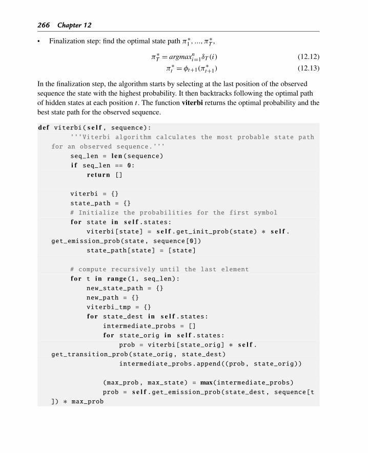
266 Chapter 12

• Finalization step: find the optimal state path π∗1 , ..., π∗

T ,

π∗T = argmaxn

i=1δT (i) (12.12)

π∗t = φt+1(π

∗t+1) (12.13)

In the finalization step, the algorithm starts by selecting at the last position of the observedsequence the state with the highest probability. It then backtracks following the optimal pathof hidden states at each position t . The function viterbi returns the optimal probability and thebest state path for the observed sequence.

def viterbi( s e l f , sequence):’’’Viterbi algorithm calculates the most probable state path

for an observed sequence.’’’

seq_len = l e n (sequence)i f seq_len == 0:

re turn []

viterbi = {}

state_path = {}

# Initialize the probabilities for the first symbol

f o r state in s e l f .states:viterbi[state] = s e l f .get_init_prob(state) ∗ s e l f .

get_emission_prob(state, sequence[0])

state_path[state] = [state]

# compute recursively until the last element

f o r t in range(1, seq_len):new_state_path = {}

new_path = {}

viterbi_tmp = {}

f o r state_dest in s e l f .states:intermediate_probs = []

f o r state_orig in s e l f .states:prob = viterbi[state_orig] ∗ s e l f .

get_transition_prob(state_orig, state_dest)

intermediate_probs.append((prob, state_orig))

(max_prob, max_state) = max(intermediate_probs)prob = s e l f .get_emission_prob(state_dest, sequence[t

]) ∗ max_prob

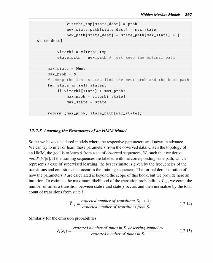
Hidden Markov Models 267

viterbi_tmp[state_dest] = prob

new_state_path[state_dest] = max_state

new_path[state_dest] = state_path[max_state] + [

state_dest]

viterbi = viterbi_tmp

state_path = new_path # just keep the optimal path

max_state = Nonemax_prob = 0

# among the last states find the best prob and the best path

f o r state in s e l f .states:i f viterbi[state] > max_prob:

max_prob = viterbi[state]

max_state = state

re turn (max_prob, state_path[max_state])

12.2.5 Learning the Parameters of an HMM Model

So far we have considered models where the respective parameters are known in advance.We can try to infer or learn these parameters from the observed data. Given the topology ofan HMM, the goal is to learn θ from a set of observed sequences, W , such that we derivemaxP [W |θ ]. If the training sequences are labeled with the corresponding state path, whichrepresents a case of supervised learning, the best estimate is given by the frequencies of thetransitions and emissions that occur in the training sequences. The formal demonstration ofhow the parameters θ are calculated is beyond the scope of this book, but we provide here anintuition. To estimate the maximum likelihood of the transition probabilities Ti,j , we count thenumber of times a transition between state i and state j occurs and then normalize by the totalcount of transitions from state i:

Ti,j = expected number of transitions Si → Sj

expected number of transitions from Si

(12.14)

Similarly for the emission probabilities:

ei (ot ) = expected number of times in Si observing symbol ot

expected number of times in Si

(12.15)

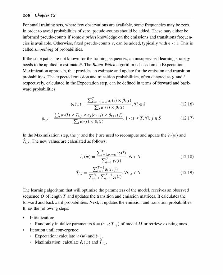
268 Chapter 12

For small training sets, where few observations are available, some frequencies may be zero.In order to avoid probabilities of zero, pseudo-counts should be added. These may either beinformed pseudo-counts if some a priori knowledge on the emissions and transitions frequen-cies is available. Otherwise, fixed pseudo-counts ε, can be added, typically with ε < 1. This iscalled smoothing of probabilities.

If the state paths are not known for the training sequences, an unsupervised learning strategyneeds to be applied to estimate θ . The Baum-Welch algorithm is based on an Expectation-Maximization approach, that provides an estimate and update for the emission and transitionprobabilities. The expected emission and transition probabilities, often denoted as γ and ξ

respectively, calculated in the Expectation step, can be defined in terms of forward and back-ward probabilities:

γi(w) =∑T

t=1,ot=w αt(i) × βt (i)∑t αt (i) × βt (i)

,∀i ∈ S (12.16)

ξi,j =∑

t αt (i) × Ti,j × ej (ot+1) × βt+1(j)∑t αt (i) × βt (i)

,1 < t ≤ T ,∀i, j ∈ S (12.17)

In the Maximization step, the γ and the ξ are used to recompute and update the ei (w) andTi,j . The new values are calculated as follows:

ei (w) =∑T

t=1,ot=w γt (i)∑Tt=1 γt (i)

,∀i ∈ S (12.18)

Ti,j =∑T −1

t=1 ξt (i, j)∑Nk=1

∑T −1t=1 γt (i)

,∀i, j ∈ S (12.19)

The learning algorithm that will optimize the parameters of the model, receives an observedsequence O of length T and updates the transition and emission matrices. It calculates theforward and backward probabilities. Next, it updates the emission and transition probabilities.It has the following steps:

• Initialization:• Randomly initialize parameters θ = (ei,a;Ti,j ) of model M or retrieve existing ones.

• Iteration until convergence:• Expectation: calculate γi(w) and ξi,j .• Maximization: calculate ei (w) and Ti,j .

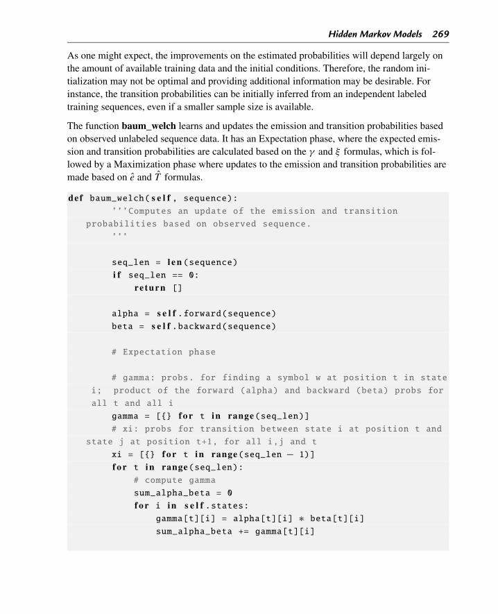
Hidden Markov Models 269

As one might expect, the improvements on the estimated probabilities will depend largely onthe amount of available training data and the initial conditions. Therefore, the random ini-tialization may not be optimal and providing additional information may be desirable. Forinstance, the transition probabilities can be initially inferred from an independent labeledtraining sequences, even if a smaller sample size is available.

The function baum_welch learns and updates the emission and transition probabilities basedon observed unlabeled sequence data. It has an Expectation phase, where the expected emis-sion and transition probabilities are calculated based on the γ and ξ formulas, which is fol-lowed by a Maximization phase where updates to the emission and transition probabilities aremade based on e and T formulas.

def baum_welch( s e l f , sequence):’’’Computes an update of the emission and transition

probabilities based on observed sequence.

’’’

seq_len = l e n (sequence)i f seq_len == 0:

re turn []

alpha = s e l f .forward(sequence)beta = s e l f .backward(sequence)

# Expectation phase

# gamma: probs. for finding a symbol w at position t in state

i; product of the forward (alpha) and backward (beta) probs for

all t and all i

gamma = [{} f o r t in range(seq_len)]# xi: probs for transition between state i at position t and

state j at position t+1, for all i,j and t

xi = [{} f o r t in range(seq_len − 1)]

f o r t in range(seq_len):# compute gamma

sum_alpha_beta = 0

f o r i in s e l f .states:gamma[t][i] = alpha[t][i] ∗ beta[t][i]sum_alpha_beta += gamma[t][i]

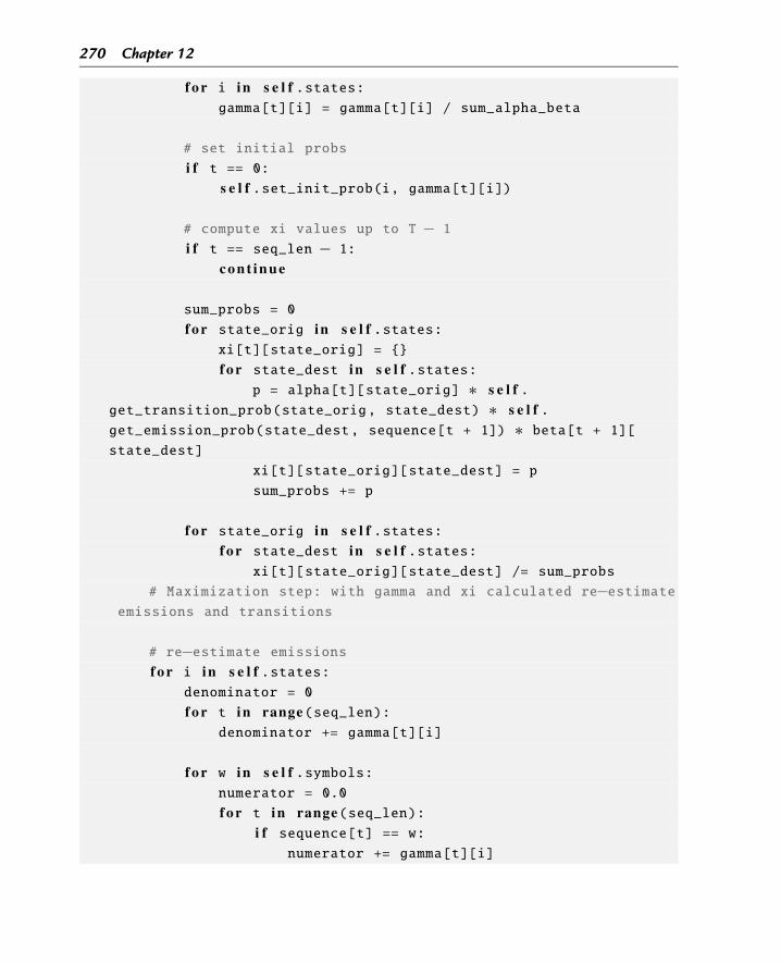
270 Chapter 12

f o r i in s e l f .states:gamma[t][i] = gamma[t][i] / sum_alpha_beta

# set initial probs

i f t == 0:s e l f .set_init_prob(i, gamma[t][i])

# compute xi values up to T − 1

i f t == seq_len − 1:

c o n t i n u e

sum_probs = 0

f o r state_orig in s e l f .states:xi[t][state_orig] = {}

f o r state_dest in s e l f .states:p = alpha[t][state_orig] ∗ s e l f .

get_transition_prob(state_orig, state_dest) ∗ s e l f .get_emission_prob(state_dest, sequence[t + 1]) ∗ beta[t + 1][state_dest]

xi[t][state_orig][state_dest] = p

sum_probs += p

f o r state_orig in s e l f .states:f o r state_dest in s e l f .states:

xi[t][state_orig][state_dest] /= sum_probs

# Maximization step: with gamma and xi calculated re−estimateemissions and transitions

# re−estimate emissionsf o r i in s e l f .states:

denominator = 0

f o r t in range(seq_len):denominator += gamma[t][i]

f o r w in s e l f .symbols:numerator = 0.0

f o r t in range(seq_len):i f sequence[t] == w:

numerator += gamma[t][i]

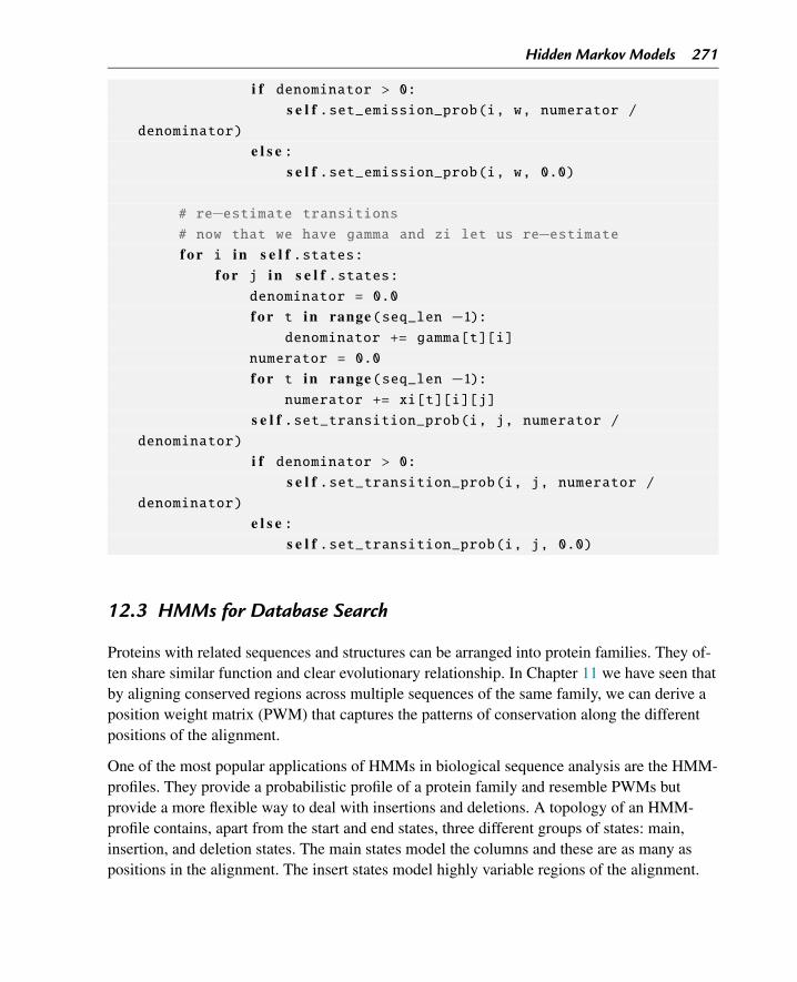
Hidden Markov Models 271

i f denominator > 0:s e l f .set_emission_prob(i, w, numerator /

denominator)

e l s e :s e l f .set_emission_prob(i, w, 0.0)

# re−estimate transitions# now that we have gamma and zi let us re−estimatef o r i in s e l f .states:

f o r j in s e l f .states:denominator = 0.0

f o r t in range(seq_len −1):denominator += gamma[t][i]

numerator = 0.0

f o r t in range(seq_len −1):numerator += xi[t][i][j]

s e l f .set_transition_prob(i, j, numerator /denominator)

i f denominator > 0:s e l f .set_transition_prob(i, j, numerator /

denominator)

e l s e :s e l f .set_transition_prob(i, j, 0.0)

12.3 HMMs for Database Search

Proteins with related sequences and structures can be arranged into protein families. They of-ten share similar function and clear evolutionary relationship. In Chapter 11 we have seen thatby aligning conserved regions across multiple sequences of the same family, we can derive aposition weight matrix (PWM) that captures the patterns of conservation along the differentpositions of the alignment.

One of the most popular applications of HMMs in biological sequence analysis are the HMM-profiles. They provide a probabilistic profile of a protein family and resemble PWMs butprovide a more flexible way to deal with insertions and deletions. A topology of an HMM-profile contains, apart from the start and end states, three different groups of states: main,insertion, and deletion states. The main states model the columns and these are as many aspositions in the alignment. The insert states model highly variable regions of the alignment.

272 Chapter 12

The deletion states, also called silent states, do not match any residue and make possible thejump between one or more columns of the alignments (corresponding to highly variable re-gions).

A typical bioinformatics application is to build an HMM-profile from a family of proteins andto search a database of sequences for other unseen family members. For an HMM-profile M

representing a protein family, all sequences W in database D are scanned. Sequences with aprobability or a score higher than a threshold are potential members of the family. The prob-ability P [W |M] can be calculated with the Forward algorithm. For further information ontheory and applications of HMM-profiles we refer the reader to the textbooks [50] and Chap-ter 4 by Anders Krogh in [6]. The Pfam database [143] contains a large collection of multiplealignments and HMM-profiles for a large number for manually verified protein families.

Bibliographic Notes and Further Reading

A general introduction to hidden Markov models can be found in [130] and Chapter 9 of [85]provides a very detailed algorithmic introduction. Materials for more oriented biological se-quence analysis with HMMs can be found in the reference textbooks [50], [6], [84] and [19].A quick introduction to the topic can be found in [54].

HMMs are very well suited for many tasks in biological sequence analysis problems. This in-cludes the tasks of gene finding, profile search, multiple sequence alignment, regulatory siteidentification and secondary structure prediction or copy-number detection. Here, we refer thereader to a few examples of applications on each of these topics. This is certainly not exhaus-tive and many other interesting works can be found elsewhere. In gene finding we emphasizethe HMMgene [90] and GENSCAN [31] methods. For HMM-profiles we refer to the seminalwork of David Haussler, Anders Krogh and colleagues [73,91], an extensive review by SeanEddy [53] and the theory behind HMM-profiles can be found in [19,50] and Chapter 4 of [6].For multiple sequence alignment with HMM the work of Sean Eddy [52] and for predictionof secondary structure from sequence [14,86]. HMMs have also been applied to detect copy-number alterations from genome sequencing data [152].

The software suite hmmer, developed by Sean Eddy, is possibly the most complete toolimplementing different methods using hidden Markov models for multiple biological se-quence analysis tasks, including searching for homologous sequences in databases and mul-tiple sequence alignments. The algorithmic details behind the methods can be found in [50]and [55–57] provide description of the different functionalities implemented in the package.

Hidden Markov Models 273

Exercises and Programming Projects

1. Adapt the code to convert probabilities into scores by taking the log2 of each probabilityand summing instead of multiplying.

2. The probability of a sequence depends directly on its length. The log-odds measure isgenerally a more convenient way to represent the score of a sequence. For an observedsequence O of length T , the measure can be defined as: logodds(O) = log P [O]

0.25T =logP [O] − T × log0.25. The 0.25 is derived from a background model where all thenucleotides are expected to occur with equal frequency.

3. Adapt the code of the Viterbi algorithm to keep track of all possible paths, returning themin addition to the optimal path.

CHAPTER 13

Graphs: Concepts and AlgorithmsIn this chapter, we present the mathematical concept of graph and its computational repre-sentation. We address some of the main algorithms over graphs and develop a set of Pythonclasses to implement different types of graphs and underlying algorithms. Graphs will be cen-tral in the development of algorithms for handling biological networks and genome assembly,tasks addressed in the next chapters.

13.1 Graphs: Definitions and Representations

A graph can be defined, in Mathematics, as a set of objects in which some of the pairs of theobjects in this set are related. While they can be easily defined and have a simple structure,they are powerful and flexible data structures, with a huge set of applications in computer sci-ence and many fields of science and engineering.

Formally, a graph G can be defined by two sets: (V ,E), where V is the set of objects, namedas vertices or nodes of the graph, and E is a set of pairs (u.v) of vertices from V , namededges or arcs, indicating the existence of a relationship between u and v.

The edges in E may have an orientation, i.e. the pairs are ordered, in which case the graph isclassified as directed, or digraph. Otherwise, the pairs are unordered and the graph is termedundirected. Another common variant is to associate numerical weights to the edges of a graph,in which case the non-existence of an edge is typically associated with the value 0 for thatweight.

It is typical to represent graphs in figures by drawing nodes as circles (or other similarshapes), and edges as lines connecting the two circles representing the vertices belongingto the corresponding node pair. These lines may have an arrow, when representing directedgraphs, indicating the direction of the edge. For weighted graphs, the weight of the edge istypically represented over the respective line. Fig. 13.1A shows a simple example, where thethree main types of graphs aforementioned are illustrated.

Graphs can be represented computationally in different ways. The choice depends on severalfactors, as the type of application of the graph and the required algorithms to be developedover them or the density of possible edges among all possible pairs of vertices. The most com-mon representations are incidence matrices and adjacency lists, while in many practical casesa combination of both might be the best solution.

Bioinformatics Algorithms. DOI: 10.1016/B978-0-12-812520-5.00013-4Copyright © 2018 Elsevier Inc. All rights reserved. 275

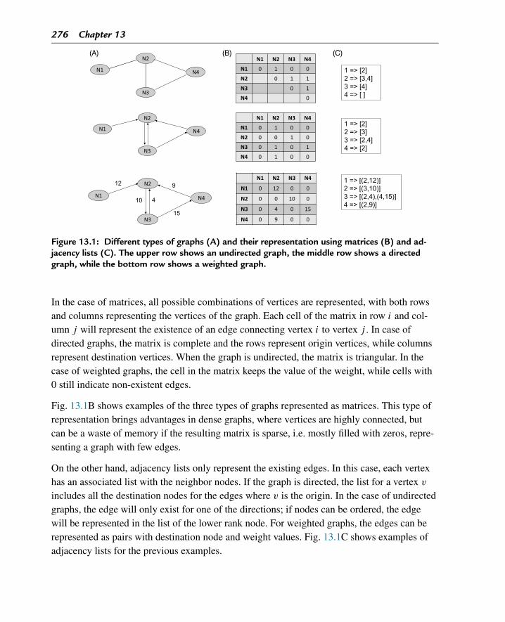
276 Chapter 13

Figure 13.1: Different types of graphs (A) and their representation using matrices (B) and ad-jacency lists (C). The upper row shows an undirected graph, the middle row shows a directedgraph, while the bottom row shows a weighted graph.

In the case of matrices, all possible combinations of vertices are represented, with both rowsand columns representing the vertices of the graph. Each cell of the matrix in row i and col-umn j will represent the existence of an edge connecting vertex i to vertex j . In case ofdirected graphs, the matrix is complete and the rows represent origin vertices, while columnsrepresent destination vertices. When the graph is undirected, the matrix is triangular. In thecase of weighted graphs, the cell in the matrix keeps the value of the weight, while cells with0 still indicate non-existent edges.

Fig. 13.1B shows examples of the three types of graphs represented as matrices. This type ofrepresentation brings advantages in dense graphs, where vertices are highly connected, butcan be a waste of memory if the resulting matrix is sparse, i.e. mostly filled with zeros, repre-senting a graph with few edges.

On the other hand, adjacency lists only represent the existing edges. In this case, each vertexhas an associated list with the neighbor nodes. If the graph is directed, the list for a vertex v

includes all the destination nodes for the edges where v is the origin. In the case of undirectedgraphs, the edge will only exist for one of the directions; if nodes can be ordered, the edgewill be represented in the list of the lower rank node. For weighted graphs, the edges can berepresented as pairs with destination node and weight values. Fig. 13.1C shows examples ofadjacency lists for the previous examples.

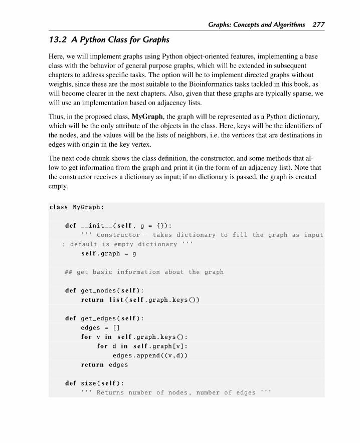
Graphs: Concepts and Algorithms 277

13.2 A Python Class for Graphs

Here, we will implement graphs using Python object-oriented features, implementing a baseclass with the behavior of general purpose graphs, which will be extended in subsequentchapters to address specific tasks. The option will be to implement directed graphs withoutweights, since these are the most suitable to the Bioinformatics tasks tackled in this book, aswill become clearer in the next chapters. Also, given that these graphs are typically sparse, wewill use an implementation based on adjacency lists.

Thus, in the proposed class, MyGraph, the graph will be represented as a Python dictionary,which will be the only attribute of the objects in the class. Here, keys will be the identifiers ofthe nodes, and the values will be the lists of neighbors, i.e. the vertices that are destinations inedges with origin in the key vertex.

The next code chunk shows the class definition, the constructor, and some methods that al-low to get information from the graph and print it (in the form of an adjacency list). Note thatthe constructor receives a dictionary as input; if no dictionary is passed, the graph is createdempty.

c l a s s MyGraph:

def __init__( s e l f , g = {}):’’’ Constructor − takes dictionary to fill the graph as input

; default is empty dictionary ’’’

s e l f .graph = g

## get basic information about the graph

def get_nodes( s e l f ):re turn l i s t ( s e l f .graph.keys())

def get_edges( s e l f ):edges = []

f o r v in s e l f .graph.keys():f o r d in s e l f .graph[v]:

edges.append((v,d))

re turn edges

def size( s e l f ):’’’ Returns number of nodes, number of edges ’’’

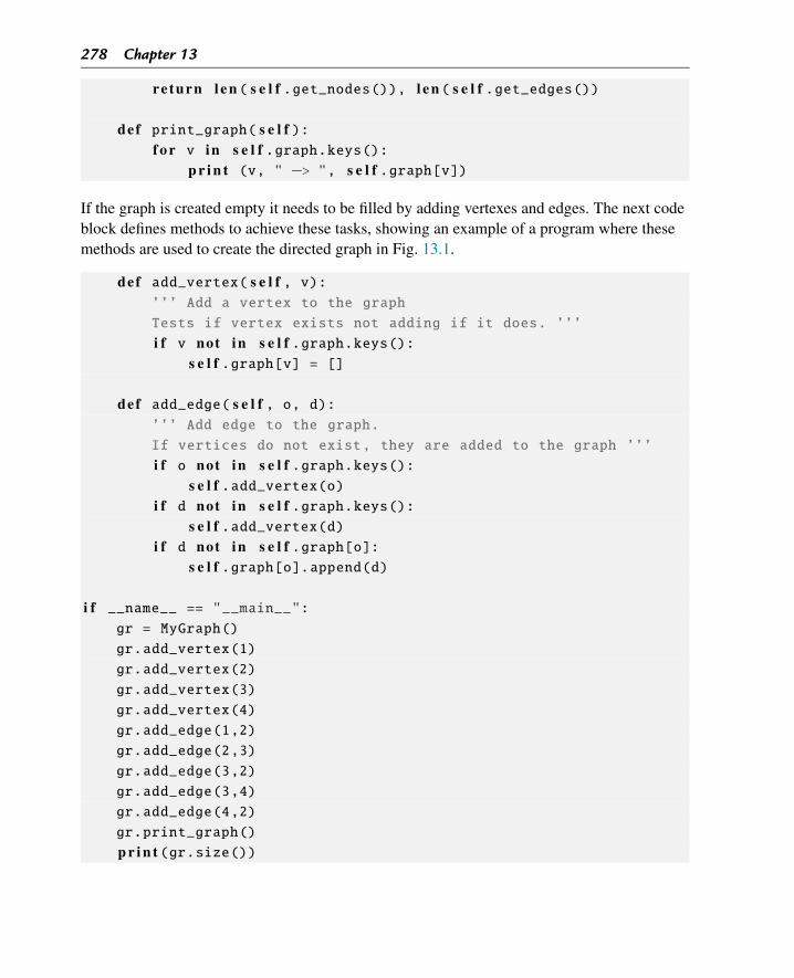
278 Chapter 13

re turn l e n ( s e l f .get_nodes()), l e n ( s e l f .get_edges())

def print_graph( s e l f ):f o r v in s e l f .graph.keys():

p r i n t (v, " −> ", s e l f .graph[v])

If the graph is created empty it needs to be filled by adding vertexes and edges. The next codeblock defines methods to achieve these tasks, showing an example of a program where thesemethods are used to create the directed graph in Fig. 13.1.

def add_vertex( s e l f , v):’’’ Add a vertex to the graph

Tests if vertex exists not adding if it does. ’’’

i f v not in s e l f .graph.keys():s e l f .graph[v] = []

def add_edge( s e l f , o, d):’’’ Add edge to the graph.

If vertices do not exist, they are added to the graph ’’’

i f o not in s e l f .graph.keys():s e l f .add_vertex(o)

i f d not in s e l f .graph.keys():s e l f .add_vertex(d)

i f d not in s e l f .graph[o]:s e l f .graph[o].append(d)

i f __name__ == "__main__":gr = MyGraph()

gr.add_vertex(1)

gr.add_vertex(2)

gr.add_vertex(3)

gr.add_vertex(4)

gr.add_edge(1,2)

gr.add_edge(2,3)

gr.add_edge(3,2)

gr.add_edge(3,4)

gr.add_edge(4,2)

gr.print_graph()

p r i n t (gr.size())

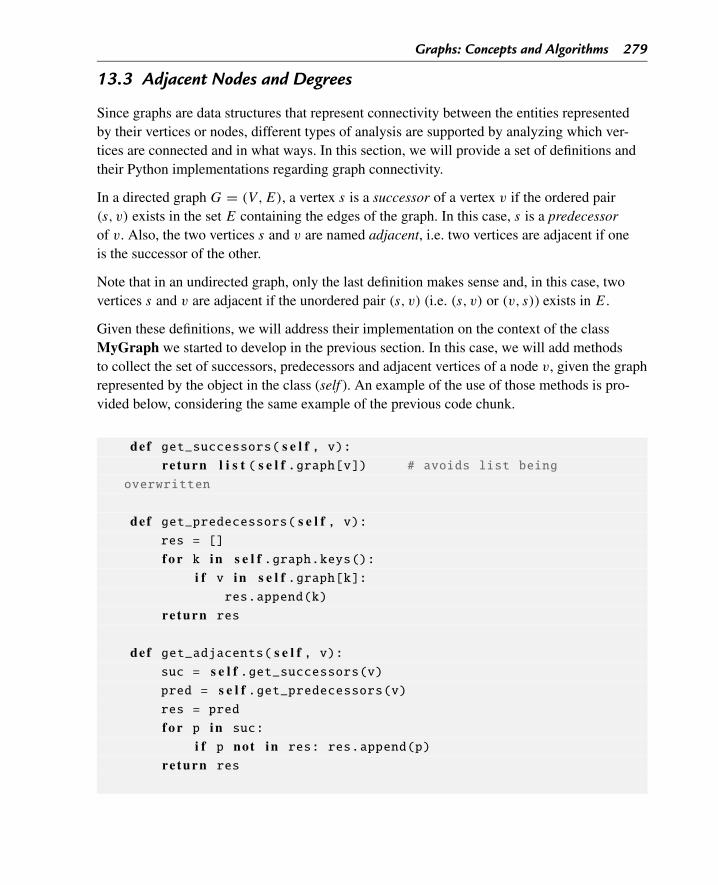
Graphs: Concepts and Algorithms 279

13.3 Adjacent Nodes and Degrees

Since graphs are data structures that represent connectivity between the entities representedby their vertices or nodes, different types of analysis are supported by analyzing which ver-tices are connected and in what ways. In this section, we will provide a set of definitions andtheir Python implementations regarding graph connectivity.

In a directed graph G = (V ,E), a vertex s is a successor of a vertex v if the ordered pair(s, v) exists in the set E containing the edges of the graph. In this case, s is a predecessorof v. Also, the two vertices s and v are named adjacent, i.e. two vertices are adjacent if oneis the successor of the other.

Note that in an undirected graph, only the last definition makes sense and, in this case, twovertices s and v are adjacent if the unordered pair (s, v) (i.e. (s, v) or (v, s)) exists in E.

Given these definitions, we will address their implementation on the context of the classMyGraph we started to develop in the previous section. In this case, we will add methodsto collect the set of successors, predecessors and adjacent vertices of a node v, given the graphrepresented by the object in the class (self ). An example of the use of those methods is pro-vided below, considering the same example of the previous code chunk.

def get_successors( s e l f , v):re turn l i s t ( s e l f .graph[v]) # avoids list being

overwritten

def get_predecessors( s e l f , v):res = []

f o r k in s e l f .graph.keys():i f v in s e l f .graph[k]:

res.append(k)

re turn res

def get_adjacents( s e l f , v):suc = s e l f .get_successors(v)pred = s e l f .get_predecessors(v)res = pred

f o r p in suc:

i f p not in res: res.append(p)

re turn res

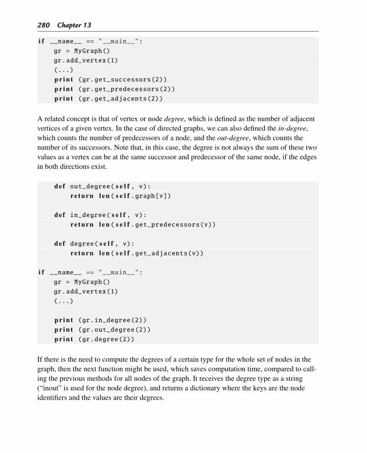
280 Chapter 13

i f __name__ == "__main__":gr = MyGraph()

gr.add_vertex(1)

(...)

p r i n t (gr.get_successors(2))p r i n t (gr.get_predecessors(2))p r i n t (gr.get_adjacents(2))

A related concept is that of vertex or node degree, which is defined as the number of adjacentvertices of a given vertex. In the case of directed graphs, we can also defined the in-degree,which counts the number of predecessors of a node, and the out-degree, which counts thenumber of its successors. Note that, in this case, the degree is not always the sum of these twovalues as a vertex can be at the same successor and predecessor of the same node, if the edgesin both directions exist.

def out_degree( s e l f , v):re turn l e n ( s e l f .graph[v])

def in_degree( s e l f , v):re turn l e n ( s e l f .get_predecessors(v))

def degree( s e l f , v):re turn l e n ( s e l f .get_adjacents(v))

i f __name__ == "__main__":gr = MyGraph()

gr.add_vertex(1)

(...)

p r i n t (gr.in_degree(2))p r i n t (gr.out_degree(2))p r i n t (gr.degree(2))

If there is the need to compute the degrees of a certain type for the whole set of nodes in thegraph, then the next function might be used, which saves computation time, compared to call-ing the previous methods for all nodes of the graph. It receives the degree type as a string(“inout” is used for the node degree), and returns a dictionary where the keys are the nodeidentifiers and the values are their degrees.

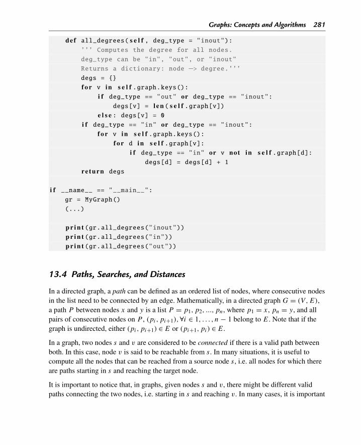
Graphs: Concepts and Algorithms 281

def all_degrees( s e l f , deg_type = "inout"):’’’ Computes the degree for all nodes.

deg_type can be "in", "out", or "inout"

Returns a dictionary: node −> degree.’’’degs = {}

f o r v in s e l f .graph.keys():i f deg_type == "out" or deg_type == "inout":

degs[v] = l e n ( s e l f .graph[v])e l s e : degs[v] = 0

i f deg_type == "in" or deg_type == "inout":f o r v in s e l f .graph.keys():

f o r d in s e l f .graph[v]:i f deg_type == "in" or v not in s e l f .graph[d]:

degs[d] = degs[d] + 1

re turn degs

i f __name__ == "__main__":gr = MyGraph()

(...)

p r i n t (gr.all_degrees("inout"))p r i n t (gr.all_degrees("in"))p r i n t (gr.all_degrees("out"))

13.4 Paths, Searches, and Distances

In a directed graph, a path can be defined as an ordered list of nodes, where consecutive nodesin the list need to be connected by an edge. Mathematically, in a directed graph G = (V ,E),a path P between nodes x and y is a list P = p1,p2, ..., pn, where p1 = x, pn = y, and allpairs of consecutive nodes on P , (pi,pi+1),∀i ∈ 1, . . . , n − 1 belong to E. Note that if thegraph is undirected, either (pi,pi+1) ∈ E or (pi+1,pi) ∈ E.

In a graph, two nodes s and v are considered to be connected if there is a valid path betweenboth. In this case, node v is said to be reachable from s. In many situations, it is useful tocompute all the nodes that can be reached from a source node s, i.e. all nodes for which thereare paths starting in s and reaching the target node.

It is important to notice that, in graphs, given nodes s and v, there might be different validpaths connecting the two nodes, i.e. starting in s and reaching v. In many cases, it is important

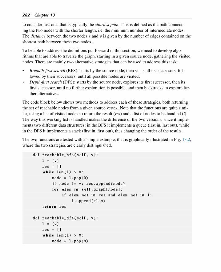
282 Chapter 13

to consider just one, that is typically the shortest path. This is defined as the path connect-ing the two nodes with the shorter length, i.e. the minimum number of intermediate nodes.The distance between the two nodes s and v is given by the number of edges contained on theshortest path between these two nodes.

To be able to address the definitions put forward in this section, we need to develop algo-rithms that are able to traverse the graph, starting in a given source node, gathering the visitednodes. There are mainly two alternative strategies that can be used to address this task:

• Breadth-first search (BFS): starts by the source node, then visits all its successors, fol-lowed by their successors, until all possible nodes are visited;

• Depth-first search (DFS): starts by the source node, explores its first successor, then itsfirst successor, until no further exploration is possible, and then backtracks to explore fur-ther alternatives.

The code block below shows two methods to address each of these strategies, both returningthe set of reachable nodes from a given source vertex. Note that the functions are quite simi-lar, using a list of visited nodes to return the result (res) and a list of nodes to be handled (l).The way this working list is handled makes the difference of the two versions, since it imple-ments two different data structures: in the BFS it implements a queue (last in, last out), whilein the DFS it implements a stack (first in, first out), thus changing the order of the results.

The two functions are tested with a simple example, that is graphically illustrated in Fig. 13.2,where the two strategies are clearly distinguished.

def reachable_bfs( s e l f , v):l = [v]

res = []

whi le l e n (l) > 0:node = l.pop(0)

i f node != v: res.append(node)f o r elem in s e l f .graph[node]:

i f elem not in res and elem not in l:

l.append(elem)

re turn res

def reachable_dfs( s e l f , v):l = [v]

res = []

whi le l e n (l) > 0:node = l.pop(0)

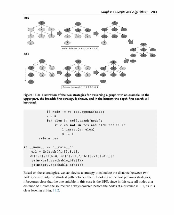
Graphs: Concepts and Algorithms 283

Figure 13.2: Illustration of the two strategies for traversing a graph with an example. In theupper part, the breadth-first strategy is shown, and in the bottom the depth-first search is il-lustrated.

i f node != v: res.append(node)s = 0

f o r elem in s e l f .graph[node]:i f elem not in res and elem not in l:

l.insert(s, elem)

s += 1

re turn res

i f __name__ == "__main__":gr2 = MyGraph({1:[2,3,4],

2:[5,6],3:[6,8],4:[8],5:[7],6:[],7:[],8:[]})

p r i n t (gr2.reachable_bfs(1))p r i n t (gr2.reachable_dfs(1))

Based on these strategies, we can devise a strategy to calculate the distance between twonodes, or similarly the shortest path between them. Looking at the two previous strategies,it becomes clear that the one suitable in this case is the BFS, since in this case all nodes at adistance of n from the source are always covered before the nodes at a distance n + 1, as it isclear looking at Fig. 13.2.

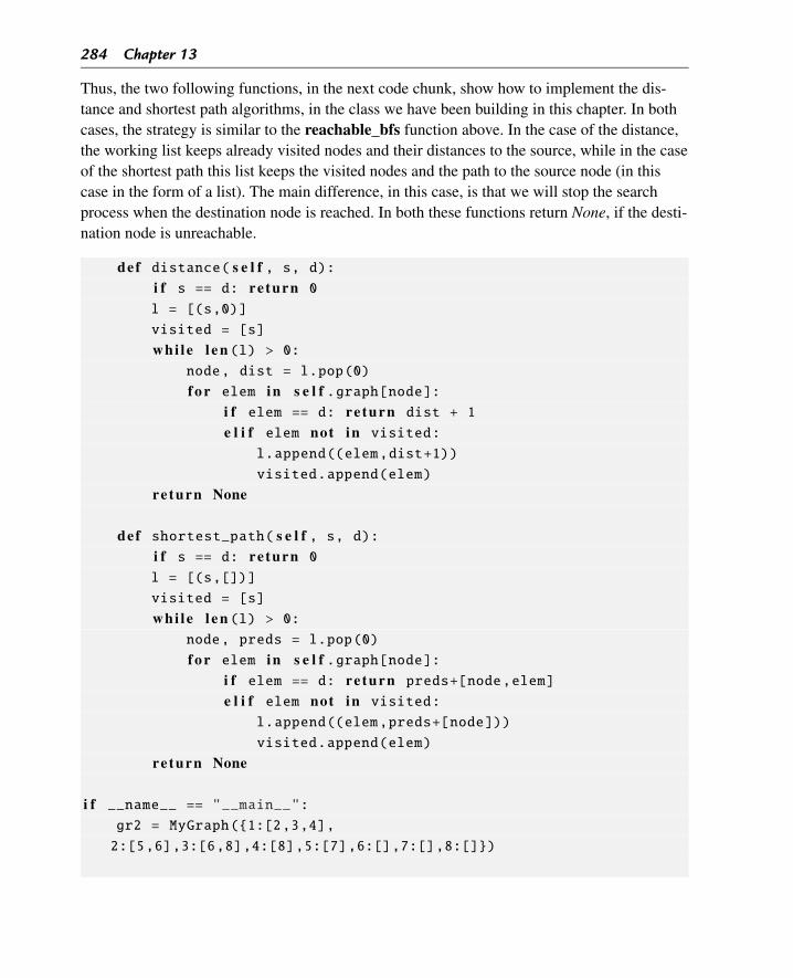
284 Chapter 13

Thus, the two following functions, in the next code chunk, show how to implement the dis-tance and shortest path algorithms, in the class we have been building in this chapter. In bothcases, the strategy is similar to the reachable_bfs function above. In the case of the distance,the working list keeps already visited nodes and their distances to the source, while in the caseof the shortest path this list keeps the visited nodes and the path to the source node (in thiscase in the form of a list). The main difference, in this case, is that we will stop the searchprocess when the destination node is reached. In both these functions return None, if the desti-nation node is unreachable.

def distance( s e l f , s, d):i f s == d: re turn 0l = [(s,0)]

visited = [s]

whi le l e n (l) > 0:node, dist = l.pop(0)

f o r elem in s e l f .graph[node]:i f elem == d: re turn dist + 1

e l i f elem not in visited:

l.append((elem,dist+1))

visited.append(elem)

re turn None

def shortest_path( s e l f , s, d):i f s == d: re turn 0l = [(s,[])]

visited = [s]

whi le l e n (l) > 0:node, preds = l.pop(0)

f o r elem in s e l f .graph[node]:i f elem == d: re turn preds+[node,elem]

e l i f elem not in visited:

l.append((elem,preds+[node]))

visited.append(elem)

re turn None

i f __name__ == "__main__":gr2 = MyGraph({1:[2,3,4],

2:[5,6],3:[6,8],4:[8],5:[7],6:[],7:[],8:[]})

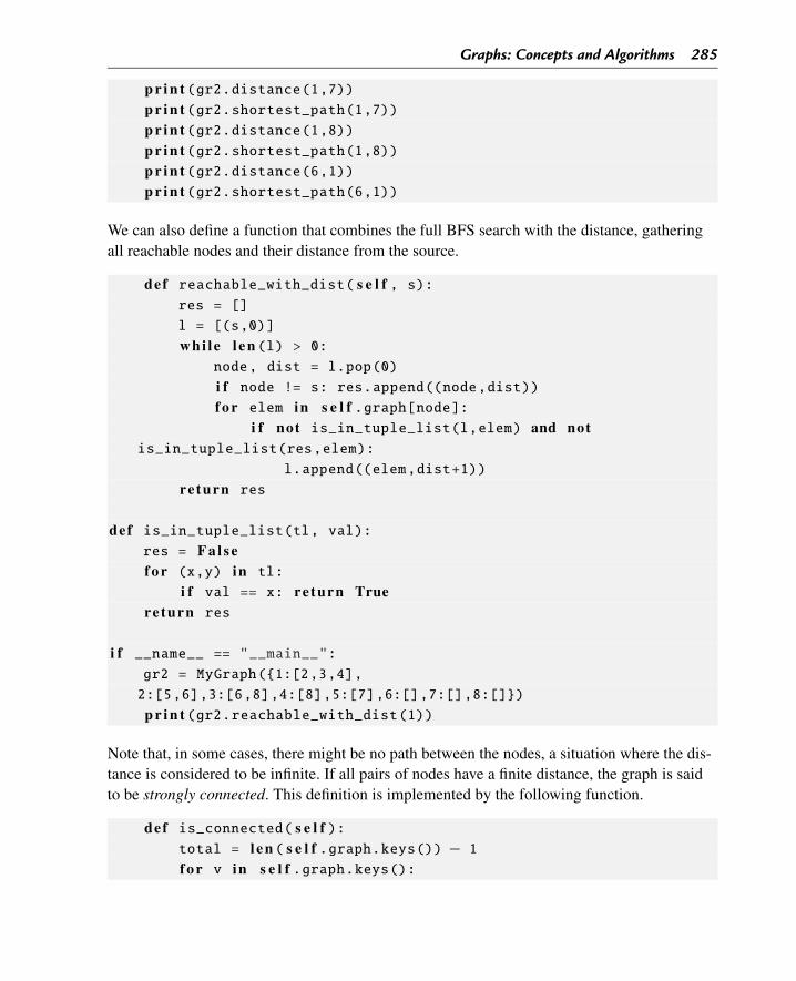
Graphs: Concepts and Algorithms 285

p r i n t (gr2.distance(1,7))p r i n t (gr2.shortest_path(1,7))p r i n t (gr2.distance(1,8))p r i n t (gr2.shortest_path(1,8))p r i n t (gr2.distance(6,1))p r i n t (gr2.shortest_path(6,1))

We can also define a function that combines the full BFS search with the distance, gatheringall reachable nodes and their distance from the source.

def reachable_with_dist( s e l f , s):res = []

l = [(s,0)]

whi le l e n (l) > 0:node, dist = l.pop(0)

i f node != s: res.append((node,dist))f o r elem in s e l f .graph[node]:

i f not is_in_tuple_list(l,elem) and notis_in_tuple_list(res,elem):

l.append((elem,dist+1))

re turn res

def is_in_tuple_list(tl, val):res = F a l s ef o r (x,y) in tl:

i f val == x: re turn Truereturn res

i f __name__ == "__main__":gr2 = MyGraph({1:[2,3,4],

2:[5,6],3:[6,8],4:[8],5:[7],6:[],7:[],8:[]})

p r i n t (gr2.reachable_with_dist(1))

Note that, in some cases, there might be no path between the nodes, a situation where the dis-tance is considered to be infinite. If all pairs of nodes have a finite distance, the graph is saidto be strongly connected. This definition is implemented by the following function.

def is_connected( s e l f ):total = l e n ( s e l f .graph.keys()) − 1

f o r v in s e l f .graph.keys():

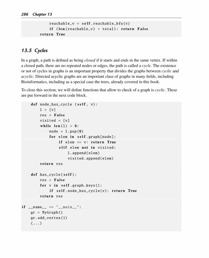
286 Chapter 13

reachable_v = s e l f .reachable_bfs(v)i f ( l e n (reachable_v) < total): re turn F a l s e

re turn True

13.5 Cycles

In a graph, a path is defined as being closed if it starts and ends in the same vertex. If withina closed path, there are no repeated nodes or edges, the path is called a cycle. The existenceor not of cycles in graphs is an important property that divides the graphs between cyclic andacyclic. Directed acyclic graphs are an important class of graphs in many fields, includingBioinformatics, including as a special case the trees, already covered in this book.

To close this section, we will define functions that allow to check of a graph is cyclic. Theseare put forward in the next code block.

def node_has_cycle ( s e l f , v):l = [v]

res = F a l s evisited = [v]

whi le l e n (l) > 0:node = l.pop(0)

f o r elem in s e l f .graph[node]:i f elem == v: re turn Truee l i f elem not in visited:

l.append(elem)

visited.append(elem)

re turn res

def has_cycle( s e l f ):res = F a l s ef o r v in s e l f .graph.keys():

i f s e l f .node_has_cycle(v): re turn Truereturn res

i f __name__ == "__main__":gr = MyGraph()

gr.add_vertex(1)

(...)

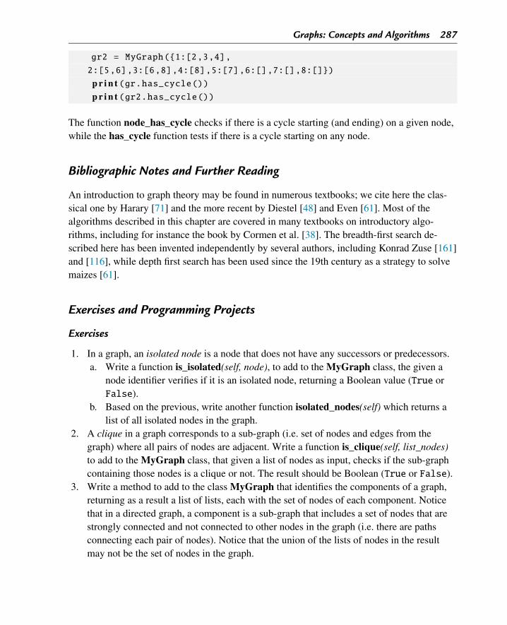
Graphs: Concepts and Algorithms 287

gr2 = MyGraph({1:[2,3,4],

2:[5,6],3:[6,8],4:[8],5:[7],6:[],7:[],8:[]})

p r i n t (gr.has_cycle())p r i n t (gr2.has_cycle())

The function node_has_cycle checks if there is a cycle starting (and ending) on a given node,while the has_cycle function tests if there is a cycle starting on any node.

Bibliographic Notes and Further Reading

An introduction to graph theory may be found in numerous textbooks; we cite here the clas-sical one by Harary [71] and the more recent by Diestel [48] and Even [61]. Most of thealgorithms described in this chapter are covered in many textbooks on introductory algo-rithms, including for instance the book by Cormen et al. [38]. The breadth-first search de-scribed here has been invented independently by several authors, including Konrad Zuse [161]and [116], while depth first search has been used since the 19th century as a strategy to solvemaizes [61].

Exercises and Programming Projects

Exercises

1. In a graph, an isolated node is a node that does not have any successors or predecessors.a. Write a function is_isolated(self, node), to add to the MyGraph class, the given a

node identifier verifies if it is an isolated node, returning a Boolean value (True orFalse).

b. Based on the previous, write another function isolated_nodes(self) which returns alist of all isolated nodes in the graph.

2. A clique in a graph corresponds to a sub-graph (i.e. set of nodes and edges from thegraph) where all pairs of nodes are adjacent. Write a function is_clique(self, list_nodes)to add to the MyGraph class, that given a list of nodes as input, checks if the sub-graphcontaining those nodes is a clique or not. The result should be Boolean (True or False).

3. Write a method to add to the class MyGraph that identifies the components of a graph,returning as a result a list of lists, each with the set of nodes of each component. Noticethat in a directed graph, a component is a sub-graph that includes a set of nodes that arestrongly connected and not connected to other nodes in the graph (i.e. there are pathsconnecting each pair of nodes). Notice that the union of the lists of nodes in the resultmay not be the set of nodes in the graph.

288 Chapter 13

Programming Projects

1. Write a class to represent undirected graphs. Check which methods from the classMyGraph still work over undirected graphs and re-implement those methods that donot apply.

2. Write a class to represent weighted directed graphs as a sub-class to the class MyGraph.Check which methods need to be redefined. Add methods to calculate shortest paths anddistances between a pair of nodes, taking into account the weights of the edges (searchfor the details of the Dijkstra algorithm if you are not familiar with this problem).

CHAPTER 14

Graphs and Biological Networks

In this chapter, we briefly review the importance of networks in biological discovery and dis-cuss how biologically relevant networks can be represented using graphs, similar to the onespresented in the last chapter. We present and implement different techniques for network topo-logical analysis, including degree distributions, mean distances, clustering coefficients andhub analysis, and discuss their relevance in biological research.

14.1 Introduction

Over the last years, different types of representations, based in the concept of graph presentedin the previous chapter, have been used to characterize and simulate different types of biolog-ical systems, mainly within cells. These graphs, globally denominated as biological networks,typically represent in their nodes biological entities, such as genes, proteins, or chemical com-pounds, while edges represent different types of interactions or relationships between theseentities, with a well-defined biological meaning (e.g. genes encoding proteins, metabolitesparticipating in reactions, proteins that regulate gene expression or bind to compounds).

These networks have provided powerful tools, within the field of Systems Biology, to supportfor the global analysis of cell organization and phenotypical behavior, and their main sub-systems with an emphasis in metabolism, gene expression regulation and signal transduction.

Metabolic networks typically encompass reactions (or their encoding enzymes) and metabo-lites (compounds involved in metabolic reactions), representing the set of (enzyme-catalyzed)chemical transformations that sustain life. These networks may include only one type of entity(either reactions/enzymes or metabolites) or include both. Fig. 14.1 represents a very simplemetabolic system and its representation in different types of networks.

On the other hand, regulatory networks encompass genes and proteins, representing the pro-cesses that allow cells to control the levels of gene expression in different situations (e.g. dif-ferent cell types or distinct stimuli), while signaling networks represent the protein cascadestypically involved in the transduction of signals from the outside of the cell to the internal reg-ulatory and metabolic systems.

Even without having the capability to support the simulation of cellular behavior directly, thestructural analysis of these networks has provided, in the last few years, some insights into

Bioinformatics Algorithms. DOI: 10.1016/B978-0-12-812520-5.00014-6Copyright © 2018 Elsevier Inc. All rights reserved. 289

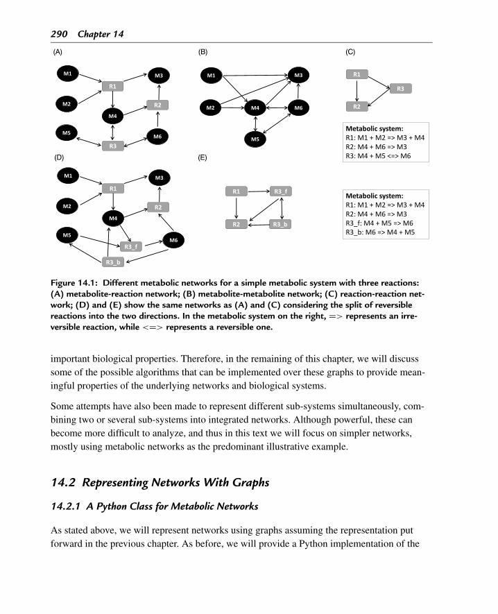
290 Chapter 14

Figure 14.1: Different metabolic networks for a simple metabolic system with three reactions:(A) metabolite-reaction network; (B) metabolite-metabolite network; (C) reaction-reaction net-work; (D) and (E) show the same networks as (A) and (C) considering the split of reversiblereactions into the two directions. In the metabolic system on the right, => represents an irre-versible reaction, while <=> represents a reversible one.

important biological properties. Therefore, in the remaining of this chapter, we will discusssome of the possible algorithms that can be implemented over these graphs to provide mean-ingful properties of the underlying networks and biological systems.

Some attempts have also been made to represent different sub-systems simultaneously, com-bining two or several sub-systems into integrated networks. Although powerful, these canbecome more difficult to analyze, and thus in this text we will focus on simpler networks,mostly using metabolic networks as the predominant illustrative example.

14.2 Representing Networks With Graphs

14.2.1 A Python Class for Metabolic Networks

As stated above, we will represent networks using graphs assuming the representation putforward in the previous chapter. As before, we will provide a Python implementation of the

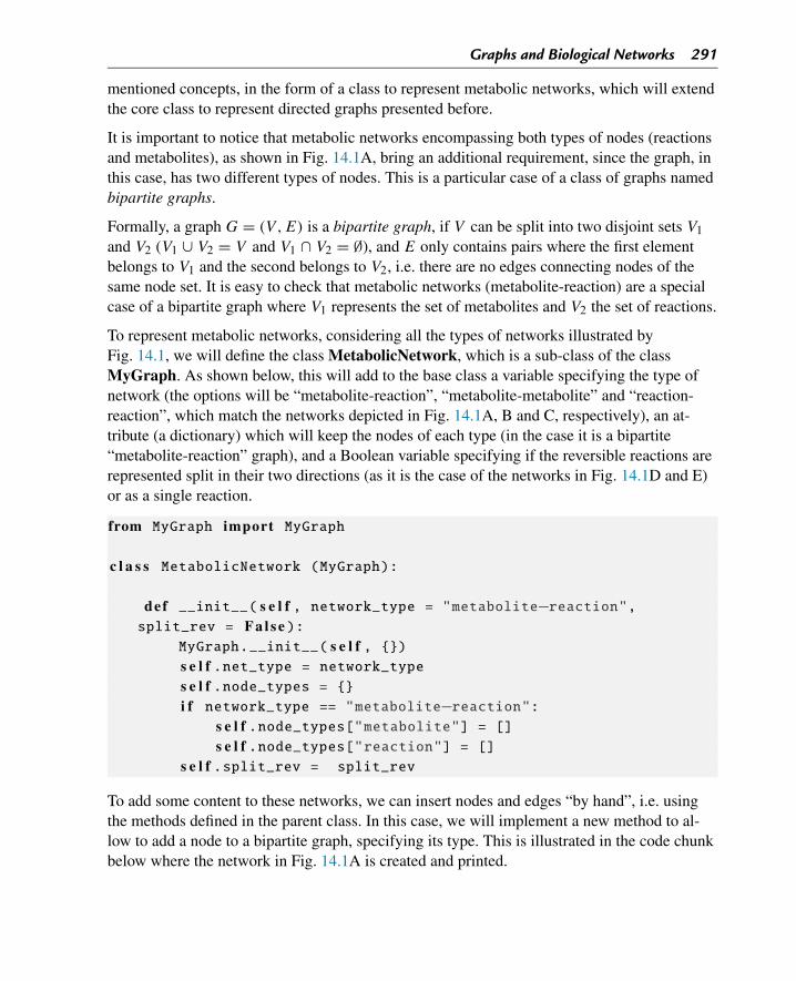
Graphs and Biological Networks 291

mentioned concepts, in the form of a class to represent metabolic networks, which will extendthe core class to represent directed graphs presented before.

It is important to notice that metabolic networks encompassing both types of nodes (reactionsand metabolites), as shown in Fig. 14.1A, bring an additional requirement, since the graph, inthis case, has two different types of nodes. This is a particular case of a class of graphs namedbipartite graphs.

Formally, a graph G = (V ,E) is a bipartite graph, if V can be split into two disjoint sets V1

and V2 (V1 ∪ V2 = V and V1 ∩ V2 = ∅), and E only contains pairs where the first elementbelongs to V1 and the second belongs to V2, i.e. there are no edges connecting nodes of thesame node set. It is easy to check that metabolic networks (metabolite-reaction) are a specialcase of a bipartite graph where V1 represents the set of metabolites and V2 the set of reactions.

To represent metabolic networks, considering all the types of networks illustrated byFig. 14.1, we will define the class MetabolicNetwork, which is a sub-class of the classMyGraph. As shown below, this will add to the base class a variable specifying the type ofnetwork (the options will be “metabolite-reaction”, “metabolite-metabolite” and “reaction-reaction”, which match the networks depicted in Fig. 14.1A, B and C, respectively), an at-tribute (a dictionary) which will keep the nodes of each type (in the case it is a bipartite“metabolite-reaction” graph), and a Boolean variable specifying if the reversible reactions arerepresented split in their two directions (as it is the case of the networks in Fig. 14.1D and E)or as a single reaction.

from MyGraph import MyGraph

c l a s s MetabolicNetwork (MyGraph):

def __init__( s e l f , network_type = "metabolite−reaction",split_rev = F a l s e ):

MyGraph.__init__( s e l f , {})s e l f .net_type = network_types e l f .node_types = {}i f network_type == "metabolite−reaction":

s e l f .node_types["metabolite"] = []s e l f .node_types["reaction"] = []

s e l f .split_rev = split_rev

To add some content to these networks, we can insert nodes and edges “by hand”, i.e. usingthe methods defined in the parent class. In this case, we will implement a new method to al-low to add a node to a bipartite graph, specifying its type. This is illustrated in the code chunkbelow where the network in Fig. 14.1A is created and printed.

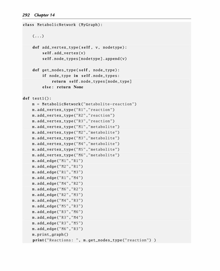
292 Chapter 14

c l a s s MetabolicNetwork (MyGraph):

(...)

def add_vertex_type( s e l f , v, nodetype):s e l f .add_vertex(v)s e l f .node_types[nodetype].append(v)

def get_nodes_type( s e l f , node_type):i f node_type in s e l f .node_types:

re turn s e l f .node_types[node_type]e l s e : re turn None

def test1():m = MetabolicNetwork("metabolite−reaction")m.add_vertex_type("R1","reaction")

m.add_vertex_type("R2","reaction")

m.add_vertex_type("R3","reaction")

m.add_vertex_type("M1","metabolite")

m.add_vertex_type("M2","metabolite")

m.add_vertex_type("M3","metabolite")

m.add_vertex_type("M4","metabolite")

m.add_vertex_type("M5","metabolite")

m.add_vertex_type("M6","metabolite")

m.add_edge("M1","R1")

m.add_edge("M2","R1")

m.add_edge("R1","M3")

m.add_edge("R1","M4")

m.add_edge("M4","R2")

m.add_edge("M6","R2")

m.add_edge("R2","M3")

m.add_edge("M4","R3")

m.add_edge("M5","R3")

m.add_edge("R3","M6")

m.add_edge("R3","M4")

m.add_edge("R3","M5")

m.add_edge("M6","R3")

m.print_graph()

p r i n t ("Reactions: ", m.get_nodes_type("reaction") )

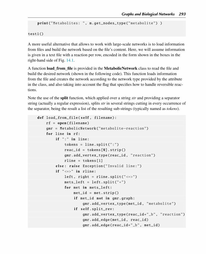
Graphs and Biological Networks 293

p r i n t ("Metabolites: ", m.get_nodes_type("metabolite") )

test1()

A more useful alternative that allows to work with large-scale networks is to load informationfrom files and build the network based on the file’s content. Here, we will assume informationis given in a text file with a reaction per row, encoded in the form shown in the boxes in theright-hand side of Fig. 14.1.

A function load_from_file is provided in the MetabolicNetwork class to read the file andbuild the desired network (shown in the following code). This function loads informationfrom the file and creates the network according to the network type provided by the attributein the class, and also taking into account the flag that specifies how to handle reversible reac-tions.

Note the use of the split function, which applied over a string str and providing a separatorstring (actually a regular expression), splits str in several strings cutting in every occurrence ofthe separator, being the result a list of the resulting sub-strings (typically named as tokens).

def load_from_file( s e l f , filename):rf = open(filename)gmr = MetabolicNetwork("metabolite−reaction")f o r line in rf:

i f ":" in line:

tokens = line.split(":")

reac_id = tokens[0].strip()

gmr.add_vertex_type(reac_id, "reaction")

rline = tokens[1]

e l s e : r a i s e Exception("Invalid line:")i f "<=>" in rline:

left, right = rline.split("<=>")

mets_left = left.split("+")

f o r met in mets_left:

met_id = met.strip()

i f met_id not in gmr.graph:

gmr.add_vertex_type(met_id, "metabolite")

i f s e l f .split_rev:gmr.add_vertex_type(reac_id+"_b", "reaction")

gmr.add_edge(met_id, reac_id)

gmr.add_edge(reac_id+"_b", met_id)

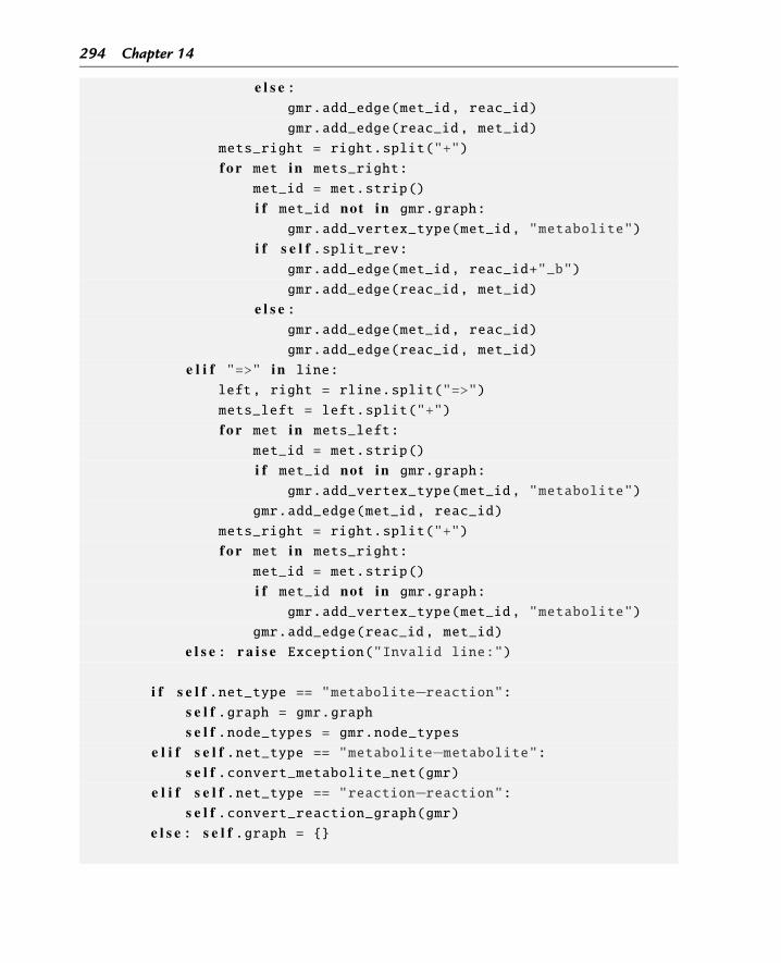
294 Chapter 14

e l s e :gmr.add_edge(met_id, reac_id)

gmr.add_edge(reac_id, met_id)

mets_right = right.split("+")

f o r met in mets_right:

met_id = met.strip()

i f met_id not in gmr.graph:

gmr.add_vertex_type(met_id, "metabolite")

i f s e l f .split_rev:gmr.add_edge(met_id, reac_id+"_b")

gmr.add_edge(reac_id, met_id)

e l s e :gmr.add_edge(met_id, reac_id)

gmr.add_edge(reac_id, met_id)

e l i f "=>" in line:

left, right = rline.split("=>")

mets_left = left.split("+")

f o r met in mets_left:

met_id = met.strip()

i f met_id not in gmr.graph:

gmr.add_vertex_type(met_id, "metabolite")

gmr.add_edge(met_id, reac_id)

mets_right = right.split("+")

f o r met in mets_right:

met_id = met.strip()

i f met_id not in gmr.graph:

gmr.add_vertex_type(met_id, "metabolite")

gmr.add_edge(reac_id, met_id)

e l s e : r a i s e Exception("Invalid line:")

i f s e l f .net_type == "metabolite−reaction":s e l f .graph = gmr.graphs e l f .node_types = gmr.node_types

e l i f s e l f .net_type == "metabolite−metabolite":s e l f .convert_metabolite_net(gmr)

e l i f s e l f .net_type == "reaction−reaction":s e l f .convert_reaction_graph(gmr)

e l s e : s e l f .graph = {}

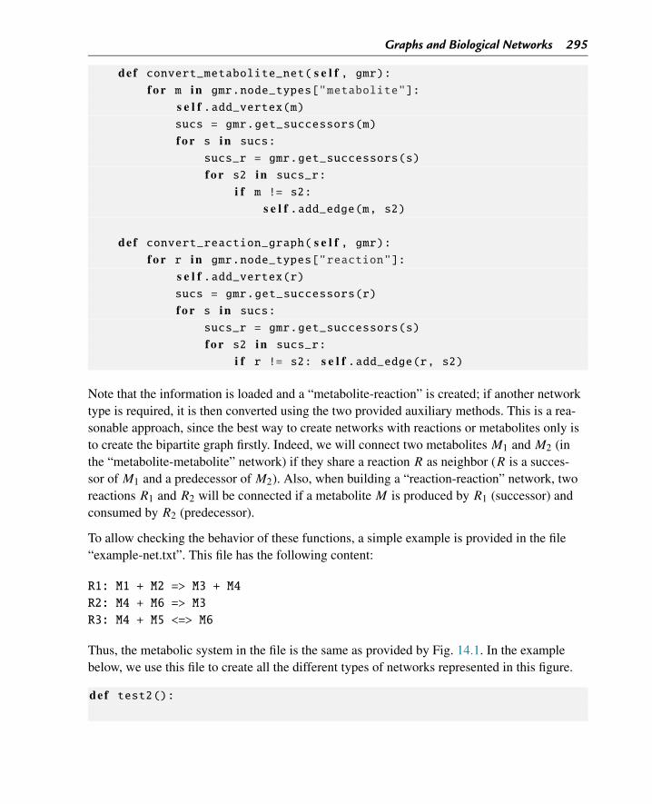
Graphs and Biological Networks 295

def convert_metabolite_net( s e l f , gmr):f o r m in gmr.node_types["metabolite"]:

s e l f .add_vertex(m)sucs = gmr.get_successors(m)

f o r s in sucs:

sucs_r = gmr.get_successors(s)

f o r s2 in sucs_r:

i f m != s2:s e l f .add_edge(m, s2)

def convert_reaction_graph( s e l f , gmr):f o r r in gmr.node_types["reaction"]:

s e l f .add_vertex(r)sucs = gmr.get_successors(r)

f o r s in sucs:

sucs_r = gmr.get_successors(s)

f o r s2 in sucs_r:

i f r != s2: s e l f .add_edge(r, s2)

Note that the information is loaded and a “metabolite-reaction” is created; if another networktype is required, it is then converted using the two provided auxiliary methods. This is a rea-sonable approach, since the best way to create networks with reactions or metabolites only isto create the bipartite graph firstly. Indeed, we will connect two metabolites M1 and M2 (inthe “metabolite-metabolite” network) if they share a reaction R as neighbor (R is a succes-sor of M1 and a predecessor of M2). Also, when building a “reaction-reaction” network, tworeactions R1 and R2 will be connected if a metabolite M is produced by R1 (successor) andconsumed by R2 (predecessor).

To allow checking the behavior of these functions, a simple example is provided in the file“example-net.txt”. This file has the following content:

R1: M1 + M2 => M3 + M4

R2: M4 + M6 => M3

R3: M4 + M5 <=> M6

Thus, the metabolic system in the file is the same as provided by Fig. 14.1. In the examplebelow, we use this file to create all the different types of networks represented in this figure.

def test2():

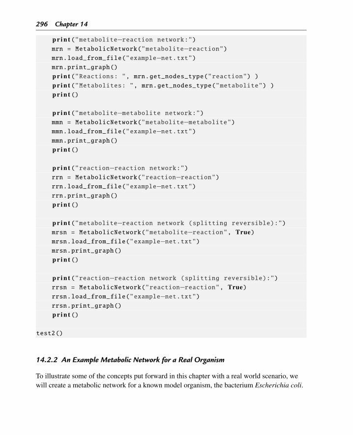
296 Chapter 14

p r i n t ("metabolite−reaction network:")mrn = MetabolicNetwork("metabolite−reaction")mrn.load_from_file("example−net.txt")mrn.print_graph()

p r i n t ("Reactions: ", mrn.get_nodes_type("reaction") )p r i n t ("Metabolites: ", mrn.get_nodes_type("metabolite") )p r i n t ()

p r i n t ("metabolite−metabolite network:")mmn = MetabolicNetwork("metabolite−metabolite")mmn.load_from_file("example−net.txt")mmn.print_graph()

p r i n t ()

p r i n t ("reaction−reaction network:")rrn = MetabolicNetwork("reaction−reaction")rrn.load_from_file("example−net.txt")rrn.print_graph()

p r i n t ()

p r i n t ("metabolite−reaction network (splitting reversible):")mrsn = MetabolicNetwork("metabolite−reaction", True)mrsn.load_from_file("example−net.txt")mrsn.print_graph()

p r i n t ()

p r i n t ("reaction−reaction network (splitting reversible):")rrsn = MetabolicNetwork("reaction−reaction", True)rrsn.load_from_file("example−net.txt")rrsn.print_graph()

p r i n t ()

test2()

14.2.2 An Example Metabolic Network for a Real Organism

To illustrate some of the concepts put forward in this chapter with a real world scenario, wewill create a metabolic network for a known model organism, the bacterium Escherichia coli.

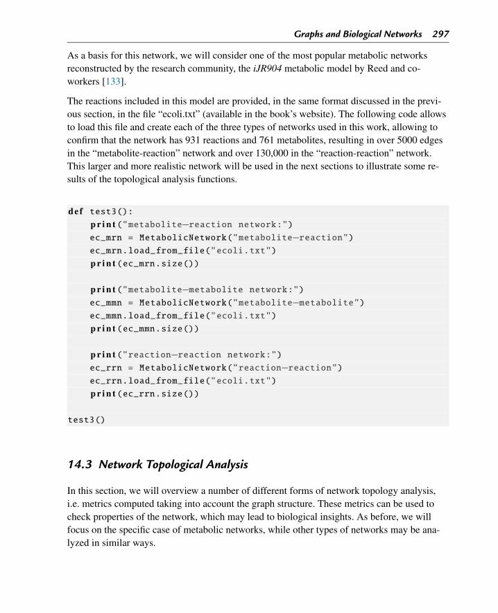
Graphs and Biological Networks 297

As a basis for this network, we will consider one of the most popular metabolic networksreconstructed by the research community, the iJR904 metabolic model by Reed and co-workers [133].

The reactions included in this model are provided, in the same format discussed in the previ-ous section, in the file “ecoli.txt” (available in the book’s website). The following code allowsto load this file and create each of the three types of networks used in this work, allowing toconfirm that the network has 931 reactions and 761 metabolites, resulting in over 5000 edgesin the “metabolite-reaction” network and over 130,000 in the “reaction-reaction” network.This larger and more realistic network will be used in the next sections to illustrate some re-sults of the topological analysis functions.

def test3():p r i n t ("metabolite−reaction network:")ec_mrn = MetabolicNetwork("metabolite−reaction")ec_mrn.load_from_file("ecoli.txt")

p r i n t (ec_mrn.size())

p r i n t ("metabolite−metabolite network:")ec_mmn = MetabolicNetwork("metabolite−metabolite")ec_mmn.load_from_file("ecoli.txt")

p r i n t (ec_mmn.size())

p r i n t ("reaction−reaction network:")ec_rrn = MetabolicNetwork("reaction−reaction")ec_rrn.load_from_file("ecoli.txt")

p r i n t (ec_rrn.size())

test3()

14.3 Network Topological Analysis

In this section, we will overview a number of different forms of network topology analysis,i.e. metrics computed taking into account the graph structure. These metrics can be used tocheck properties of the network, which may lead to biological insights. As before, we willfocus on the specific case of metabolic networks, while other types of networks may be ana-lyzed in similar ways.

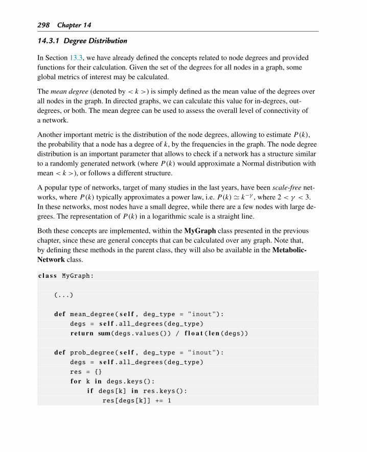
298 Chapter 14

14.3.1 Degree Distribution

In Section 13.3, we have already defined the concepts related to node degrees and providedfunctions for their calculation. Given the set of the degrees for all nodes in a graph, someglobal metrics of interest may be calculated.

The mean degree (denoted by < k >) is simply defined as the mean value of the degrees overall nodes in the graph. In directed graphs, we can calculate this value for in-degrees, out-degrees, or both. The mean degree can be used to assess the overall level of connectivity ofa network.

Another important metric is the distribution of the node degrees, allowing to estimate P(k),the probability that a node has a degree of k, by the frequencies in the graph. The node degreedistribution is an important parameter that allows to check if a network has a structure similarto a randomly generated network (where P(k) would approximate a Normal distribution withmean < k >), or follows a different structure.

A popular type of networks, target of many studies in the last years, have been scale-free net-works, where P(k) typically approximates a power law, i.e. P(k) � k−γ , where 2 < γ < 3.In these networks, most nodes have a small degree, while there are a few nodes with large de-grees. The representation of P(k) in a logarithmic scale is a straight line.

Both these concepts are implemented, within the MyGraph class presented in the previouschapter, since these are general concepts that can be calculated over any graph. Note that,by defining these methods in the parent class, they will also be available in the Metabolic-Network class.

c l a s s MyGraph:

(...)

def mean_degree( s e l f , deg_type = "inout"):degs = s e l f .all_degrees(deg_type)re turn sum(degs.values()) / f l o a t ( l e n (degs))

def prob_degree( s e l f , deg_type = "inout"):degs = s e l f .all_degrees(deg_type)res = {}

f o r k in degs.keys():

i f degs[k] in res.keys():

res[degs[k]] += 1

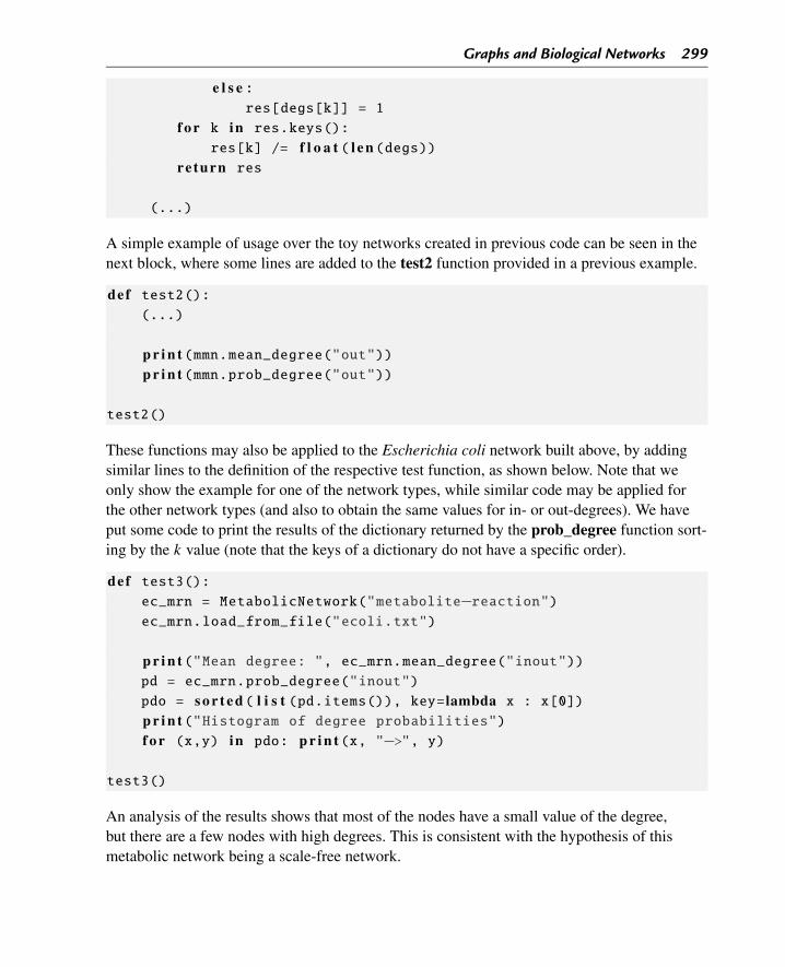
Graphs and Biological Networks 299

e l s e :res[degs[k]] = 1

f o r k in res.keys():

res[k] /= f l o a t ( l e n (degs))re turn res

(...)

A simple example of usage over the toy networks created in previous code can be seen in thenext block, where some lines are added to the test2 function provided in a previous example.

def test2():(...)

p r i n t (mmn.mean_degree("out"))p r i n t (mmn.prob_degree("out"))

test2()

These functions may also be applied to the Escherichia coli network built above, by addingsimilar lines to the definition of the respective test function, as shown below. Note that weonly show the example for one of the network types, while similar code may be applied forthe other network types (and also to obtain the same values for in- or out-degrees). We haveput some code to print the results of the dictionary returned by the prob_degree function sort-ing by the k value (note that the keys of a dictionary do not have a specific order).

def test3():ec_mrn = MetabolicNetwork("metabolite−reaction")ec_mrn.load_from_file("ecoli.txt")

p r i n t ("Mean degree: ", ec_mrn.mean_degree("inout"))pd = ec_mrn.prob_degree("inout")

pdo = s o r t e d ( l i s t (pd.items()), key= lambda x : x[0])p r i n t ("Histogram of degree probabilities")f o r (x,y) in pdo: p r i n t (x, "−>", y)

test3()

An analysis of the results shows that most of the nodes have a small value of the degree,but there are a few nodes with high degrees. This is consistent with the hypothesis of thismetabolic network being a scale-free network.

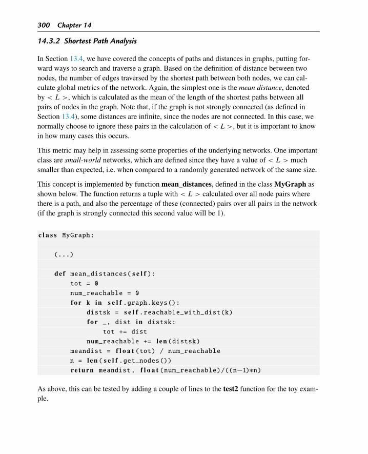
300 Chapter 14

14.3.2 Shortest Path Analysis

In Section 13.4, we have covered the concepts of paths and distances in graphs, putting for-ward ways to search and traverse a graph. Based on the definition of distance between twonodes, the number of edges traversed by the shortest path between both nodes, we can cal-culate global metrics of the network. Again, the simplest one is the mean distance, denotedby < L >, which is calculated as the mean of the length of the shortest paths between allpairs of nodes in the graph. Note that, if the graph is not strongly connected (as defined inSection 13.4), some distances are infinite, since the nodes are not connected. In this case, wenormally choose to ignore these pairs in the calculation of < L >, but it is important to knowin how many cases this occurs.

This metric may help in assessing some properties of the underlying networks. One importantclass are small-world networks, which are defined since they have a value of < L > muchsmaller than expected, i.e. when compared to a randomly generated network of the same size.

This concept is implemented by function mean_distances, defined in the class MyGraph asshown below. The function returns a tuple with < L > calculated over all node pairs wherethere is a path, and also the percentage of these (connected) pairs over all pairs in the network(if the graph is strongly connected this second value will be 1).

c l a s s MyGraph:

(...)

def mean_distances( s e l f ):tot = 0

num_reachable = 0

f o r k in s e l f .graph.keys():distsk = s e l f .reachable_with_dist(k)f o r _, dist in distsk:

tot += dist

num_reachable += l e n (distsk)meandist = f l o a t (tot) / num_reachablen = l e n ( s e l f .get_nodes())re turn meandist, f l o a t (num_reachable)/((n−1)∗n)

As above, this can be tested by adding a couple of lines to the test2 function for the toy exam-ple.

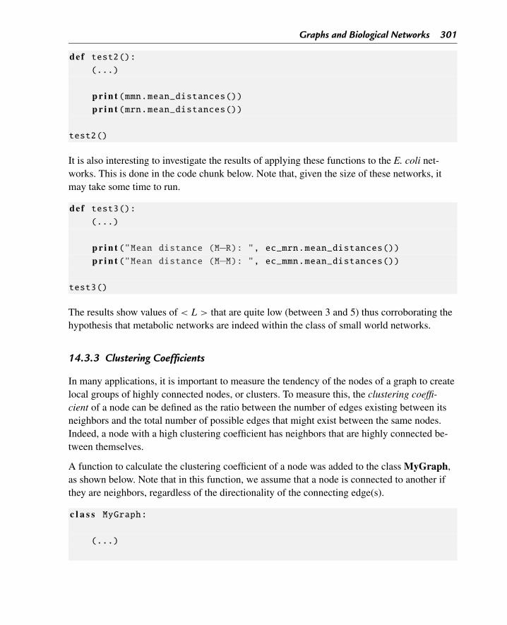
Graphs and Biological Networks 301

def test2():(...)

p r i n t (mmn.mean_distances())p r i n t (mrn.mean_distances())

test2()

It is also interesting to investigate the results of applying these functions to the E. coli net-works. This is done in the code chunk below. Note that, given the size of these networks, itmay take some time to run.

def test3():(...)

p r i n t ("Mean distance (M−R): ", ec_mrn.mean_distances())p r i n t ("Mean distance (M−M): ", ec_mmn.mean_distances())

test3()

The results show values of < L > that are quite low (between 3 and 5) thus corroborating thehypothesis that metabolic networks are indeed within the class of small world networks.

14.3.3 Clustering Coefficients

In many applications, it is important to measure the tendency of the nodes of a graph to createlocal groups of highly connected nodes, or clusters. To measure this, the clustering coeffi-cient of a node can be defined as the ratio between the number of edges existing between itsneighbors and the total number of possible edges that might exist between the same nodes.Indeed, a node with a high clustering coefficient has neighbors that are highly connected be-tween themselves.

A function to calculate the clustering coefficient of a node was added to the class MyGraph,as shown below. Note that in this function, we assume that a node is connected to another ifthey are neighbors, regardless of the directionality of the connecting edge(s).

c l a s s MyGraph:

(...)

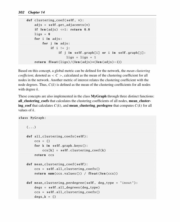
302 Chapter 14

def clustering_coef( s e l f , v):adjs = s e l f .get_adjacents(v)i f l e n (adjs) <=1: re turn 0.0

ligs = 0

f o r i in adjs:

f o r j in adjs:

i f i != j:i f j in s e l f .graph[i] or i in s e l f .graph[j]:

ligs = ligs + 1

re turn f l o a t (ligs)/( l e n (adjs)∗( l e n (adjs)−1))

Based on this concept, a global metric can be defined for the network, the mean clusteringcoefficient, denoted as < C >, calculated as the mean of the clustering coefficient for allnodes in the network. Another metric of interest relates the clustering coefficient with thenode degrees. Thus, C(k) is defined as the mean of the clustering coefficients for all nodeswith degree k.

These concepts are also implemented in the class MyGraph through three distinct functions:all_clustering_coefs that calculates the clustering coefficients of all nodes, mean_cluster-ing_coef that calculates C(k), and mean_clustering_perdegree that computes C(k) for allvalues of k.

c l a s s MyGraph:

(...)

def all_clustering_coefs( s e l f ):ccs = {}

f o r k in s e l f .graph.keys():ccs[k] = s e l f .clustering_coef(k)

re turn ccs

def mean_clustering_coef( s e l f ):ccs = s e l f .all_clustering_coefs()re turn sum(ccs.values()) / f l o a t ( l e n (ccs))

def mean_clustering_perdegree( s e l f , deg_type = "inout"):degs = s e l f .all_degrees(deg_type)ccs = s e l f .all_clustering_coefs()degs_k = {}

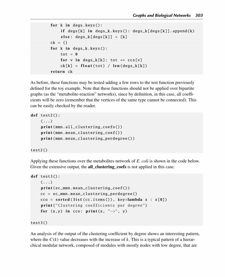
Graphs and Biological Networks 303

f o r k in degs.keys():

i f degs[k] in degs_k.keys(): degs_k[degs[k]].append(k)

e l s e : degs_k[degs[k]] = [k]ck = {}

f o r k in degs_k.keys():

tot = 0

f o r v in degs_k[k]: tot += ccs[v]

ck[k] = f l o a t (tot) / l e n (degs_k[k])re turn ck

As before, these functions may be tested adding a few rows to the test function previouslydefined for the toy example. Note that these functions should not be applied over bipartitegraphs (as the “metabolite-reaction” networks), since by definition, in this case, all coeffi-cients will be zero (remember that the vertices of the same type cannot be connected). Thiscan be easily checked by the reader.

def test2():(...)

p r i n t (mmn.all_clustering_coefs())p r i n t (mmn.mean_clustering_coef())p r i n t (mmn.mean_clustering_perdegree())

test2()

Applying these functions over the metabolites network of E. coli is shown in the code below.Given the extensive output, the all_clustering_coefs is not applied in this case.

def test3():(...)

p r i n t (ec_mmn.mean_clustering_coef())cc = ec_mmn.mean_clustering_perdegree()

cco = s o r t e d ( l i s t (cc.items()), key= lambda x : x[0])p r i n t ("Clustering coefficients per degree")f o r (x,y) in cco: p r i n t (x, "−>", y)

test3()

An analysis of the output of the clustering coefficient by degree shows an interesting pattern,where the C(k) value decreases with the increase of k. This is a typical pattern of a hierar-chical modular network, composed of modules with mostly nodes with low degree, that are

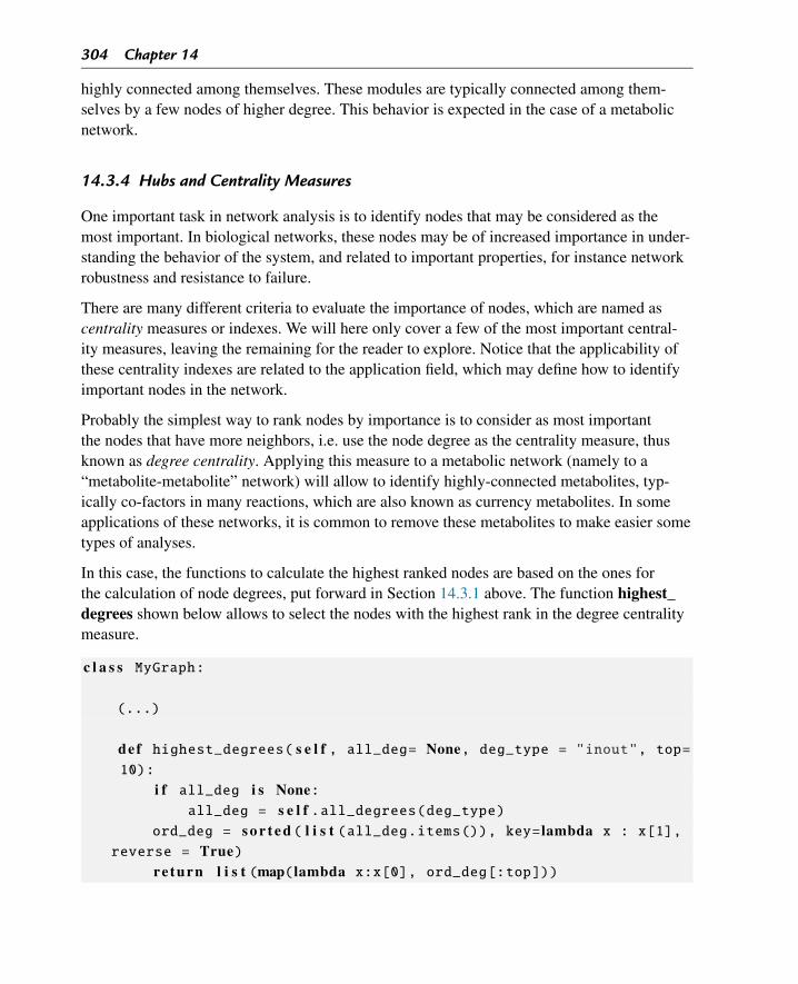
304 Chapter 14

highly connected among themselves. These modules are typically connected among them-selves by a few nodes of higher degree. This behavior is expected in the case of a metabolicnetwork.

14.3.4 Hubs and Centrality Measures

One important task in network analysis is to identify nodes that may be considered as themost important. In biological networks, these nodes may be of increased importance in under-standing the behavior of the system, and related to important properties, for instance networkrobustness and resistance to failure.

There are many different criteria to evaluate the importance of nodes, which are named ascentrality measures or indexes. We will here only cover a few of the most important central-ity measures, leaving the remaining for the reader to explore. Notice that the applicability ofthese centrality indexes are related to the application field, which may define how to identifyimportant nodes in the network.

Probably the simplest way to rank nodes by importance is to consider as most importantthe nodes that have more neighbors, i.e. use the node degree as the centrality measure, thusknown as degree centrality. Applying this measure to a metabolic network (namely to a“metabolite-metabolite” network) will allow to identify highly-connected metabolites, typ-ically co-factors in many reactions, which are also known as currency metabolites. In someapplications of these networks, it is common to remove these metabolites to make easier sometypes of analyses.

In this case, the functions to calculate the highest ranked nodes are based on the ones forthe calculation of node degrees, put forward in Section 14.3.1 above. The function highest_degrees shown below allows to select the nodes with the highest rank in the degree centralitymeasure.

c l a s s MyGraph:

(...)

def highest_degrees( s e l f , all_deg= None, deg_type = "inout", top=10):

i f all_deg i s None:all_deg = s e l f .all_degrees(deg_type)

ord_deg = s o r t e d ( l i s t (all_deg.items()), key= lambda x : x[1],reverse = True)

re turn l i s t (map( lambda x:x[0], ord_deg[:top]))

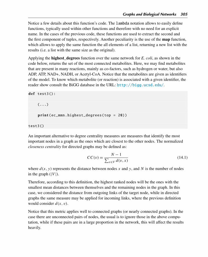
Graphs and Biological Networks 305

Notice a few details about this function’s code. The lambda notation allows to easily definefunctions, typically used within other functions and therefore with no need for an explicitname. In the cases of the previous code, these functions are used to extract the second andthe first component of tuples, respectively. Another peculiarity is the use of the map function,which allows to apply the same function the all elements of a list, returning a new list with theresults (i.e. a list with the same size as the original).

Applying the highest_degrees function over the same network for E. coli, as shown in thecode below, returns the set of the most connected metabolites. Here, we may find metabolitesthat are present in many reactions, mainly as co-factors, such as hydrogen or water, but alsoADP, ATP, NAD+, NADH, or Acetyl-CoA. Notice that the metabolites are given as identifiersof the model. To know which metabolite (or reaction) is associated with a given identifier, thereader show consult the BiGG database in the URL: http://bigg.ucsd.edu/.

def test3():

(...)

p r i n t (ec_mmn.highest_degrees(top = 20))

test3()

An important alternative to degree centrality measures are measures that identify the mostimportant nodes in a graph as the ones which are closest to the other nodes. The normalizedcloseness centrality for directed graphs may be defined as:

CC(v) = N − 1∑x∈V d(v, x)

(14.1)

where d(x, y) represents the distance between nodes x and y, and N is the number of nodesin the graph (|V |).Therefore, according to this definition, the highest ranked nodes will be the ones with thesmallest mean distances between themselves and the remaining nodes in the graph. In thiscase, we considered the distance from outgoing links of the target node, while in directedgraphs the same measure may be applied for incoming links, where the previous definitionwould consider d(x, v).

Notice that this metric applies well to connected graphs (or nearly connected graphs). In thecase there are unconnected pairs of nodes, the usual is to ignore those in the above compu-tation, while if these pairs are in a large proportion in the network, this will affect the resultsheavily.

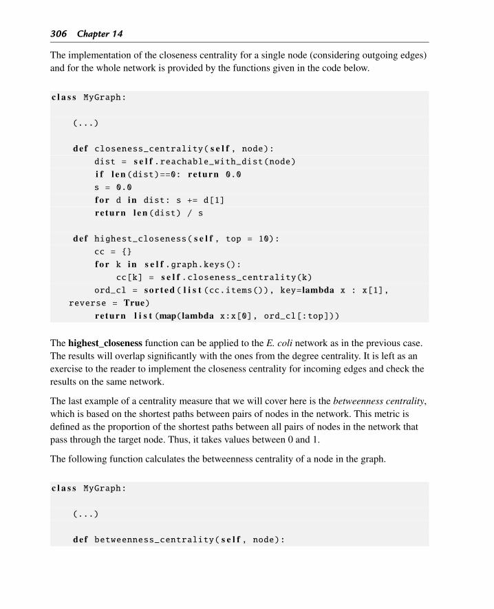
306 Chapter 14

The implementation of the closeness centrality for a single node (considering outgoing edges)and for the whole network is provided by the functions given in the code below.

c l a s s MyGraph:

(...)

def closeness_centrality( s e l f , node):dist = s e l f .reachable_with_dist(node)i f l e n (dist)==0: re turn 0.0

s = 0.0

f o r d in dist: s += d[1]

re turn l e n (dist) / s

def highest_closeness( s e l f , top = 10):cc = {}

f o r k in s e l f .graph.keys():cc[k] = s e l f .closeness_centrality(k)

ord_cl = s o r t e d ( l i s t (cc.items()), key= lambda x : x[1],reverse = True)

re turn l i s t (map( lambda x:x[0], ord_cl[:top]))

The highest_closeness function can be applied to the E. coli network as in the previous case.The results will overlap significantly with the ones from the degree centrality. It is left as anexercise to the reader to implement the closeness centrality for incoming edges and check theresults on the same network.

The last example of a centrality measure that we will cover here is the betweenness centrality,which is based on the shortest paths between pairs of nodes in the network. This metric isdefined as the proportion of the shortest paths between all pairs of nodes in the network thatpass through the target node. Thus, it takes values between 0 and 1.

The following function calculates the betweenness centrality of a node in the graph.

c l a s s MyGraph:

(...)

def betweenness_centrality( s e l f , node):

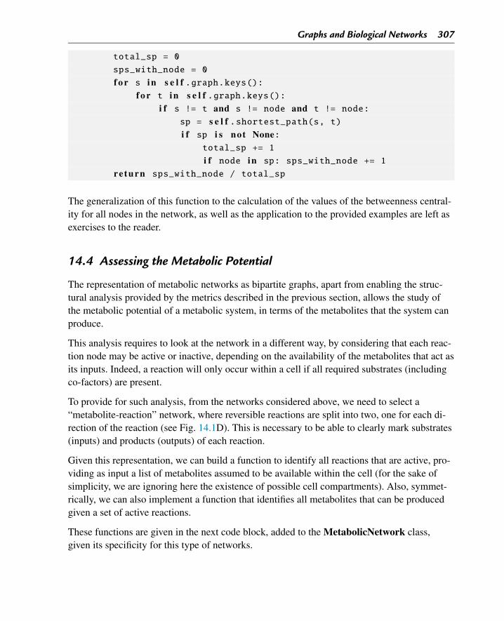
Graphs and Biological Networks 307

total_sp = 0

sps_with_node = 0

f o r s in s e l f .graph.keys():f o r t in s e l f .graph.keys():

i f s != t and s != node and t != node:sp = s e l f .shortest_path(s, t)i f sp i s not None:

total_sp += 1

i f node in sp: sps_with_node += 1

re turn sps_with_node / total_sp

The generalization of this function to the calculation of the values of the betweenness central-ity for all nodes in the network, as well as the application to the provided examples are left asexercises to the reader.

14.4 Assessing the Metabolic Potential

The representation of metabolic networks as bipartite graphs, apart from enabling the struc-tural analysis provided by the metrics described in the previous section, allows the study ofthe metabolic potential of a metabolic system, in terms of the metabolites that the system canproduce.

This analysis requires to look at the network in a different way, by considering that each reac-tion node may be active or inactive, depending on the availability of the metabolites that act asits inputs. Indeed, a reaction will only occur within a cell if all required substrates (includingco-factors) are present.

To provide for such analysis, from the networks considered above, we need to select a“metabolite-reaction” network, where reversible reactions are split into two, one for each di-rection of the reaction (see Fig. 14.1D). This is necessary to be able to clearly mark substrates(inputs) and products (outputs) of each reaction.

Given this representation, we can build a function to identify all reactions that are active, pro-viding as input a list of metabolites assumed to be available within the cell (for the sake ofsimplicity, we are ignoring here the existence of possible cell compartments). Also, symmet-rically, we can also implement a function that identifies all metabolites that can be producedgiven a set of active reactions.

These functions are given in the next code block, added to the MetabolicNetwork class,given its specificity for this type of networks.

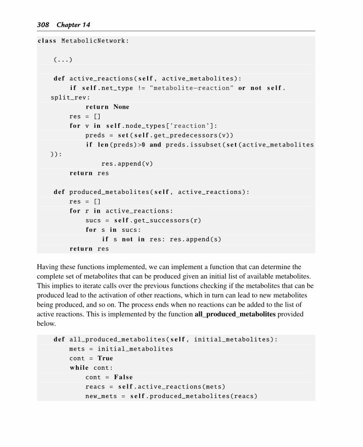
308 Chapter 14

c l a s s MetabolicNetwork:

(...)

def active_reactions( s e l f , active_metabolites):i f s e l f .net_type != "metabolite−reaction" or not s e l f .

split_rev:

re turn Noneres = []

f o r v in s e l f .node_types[’reaction’]:preds = s e t ( s e l f .get_predecessors(v))i f l e n (preds)>0 and preds.issubset( s e t (active_metabolites

)):

res.append(v)

re turn res

def produced_metabolites( s e l f , active_reactions):res = []

f o r r in active_reactions:

sucs = s e l f .get_successors(r)f o r s in sucs:

i f s not in res: res.append(s)

re turn res

Having these functions implemented, we can implement a function that can determine thecomplete set of metabolites that can be produced given an initial list of available metabolites.This implies to iterate calls over the previous functions checking if the metabolites that can beproduced lead to the activation of other reactions, which in turn can lead to new metabolitesbeing produced, and so on. The process ends when no reactions can be added to the list ofactive reactions. This is implemented by the function all_produced_metabolites providedbelow.

def all_produced_metabolites( s e l f , initial_metabolites):mets = initial_metabolites

cont = Truewhi l e cont:

cont = F a l s ereacs = s e l f .active_reactions(mets)new_mets = s e l f .produced_metabolites(reacs)

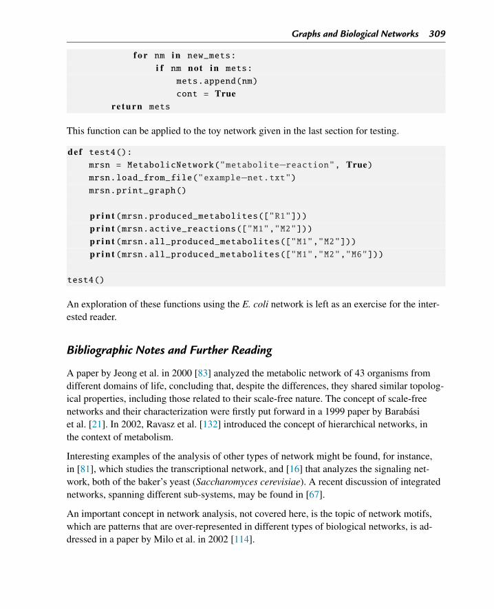
Graphs and Biological Networks 309

f o r nm in new_mets:

i f nm not in mets:

mets.append(nm)

cont = Truereturn mets

This function can be applied to the toy network given in the last section for testing.

def test4():mrsn = MetabolicNetwork("metabolite−reaction", True)mrsn.load_from_file("example−net.txt")mrsn.print_graph()

p r i n t (mrsn.produced_metabolites(["R1"]))p r i n t (mrsn.active_reactions(["M1","M2"]))p r i n t (mrsn.all_produced_metabolites(["M1","M2"]))p r i n t (mrsn.all_produced_metabolites(["M1","M2","M6"]))

test4()

An exploration of these functions using the E. coli network is left as an exercise for the inter-ested reader.

Bibliographic Notes and Further Reading

A paper by Jeong et al. in 2000 [83] analyzed the metabolic network of 43 organisms fromdifferent domains of life, concluding that, despite the differences, they shared similar topolog-ical properties, including those related to their scale-free nature. The concept of scale-freenetworks and their characterization were firstly put forward in a 1999 paper by Barabásiet al. [21]. In 2002, Ravasz et al. [132] introduced the concept of hierarchical networks, inthe context of metabolism.

Interesting examples of the analysis of other types of network might be found, for instance,in [81], which studies the transcriptional network, and [16] that analyzes the signaling net-work, both of the baker’s yeast (Saccharomyces cerevisiae). A recent discussion of integratednetworks, spanning different sub-systems, may be found in [67].

An important concept in network analysis, not covered here, is the topic of network motifs,which are patterns that are over-represented in different types of biological networks, is ad-dressed in a paper by Milo et al. in 2002 [114].

310 Chapter 14

Barabási and Olivai wrote, in 2004 [23], a very comprehensive review on the field of net-work biology, where they review these results over metabolic networks, but also considerother types of biological networks, considering their properties and discussing their evolu-tionary origin. In a more recent review, the same author and colleagues have published a veryinteresting review on some applications of network biology related methods to medical re-search [22].

Finally, many other representation formalisms, many based in graphs, have been used tomodel cells and their sub-systems in the wider field of Systems Biology, many of those al-lowing for methods to perform several types of simulation leading to phenotype prediction.An interesting review of such paradigms has been done in [106].

Exercises and Programming Projects

Exercises

1. Considering the networks of the type “metabolite-reaction” presented in this chapter,which correspond to bipartite graphs, write a method to add to the class Metabolic-Network that can detect the set of “final” metabolites, those that are produced by at leastone reaction, but are not consumed by any reaction in the network.

2. Write a method to add to the class MetabolicNetwork that, given a set of initial metabo-lites (assumed to be available) and a target metabolite, returns the shortest path to pro-duce the target metabolite, i.e. the shortest list of reactions that activated in that orderallow to produce the target metabolite from the initial set of metabolites. The reactions inthe list are only valid if they can be active in the given order (i.e. all their substrates ex-ist). The method returns None if the target metabolite cannot be produced from the list ofinitial metabolites.

Programming Projects

1. Considering the class to implement undirected graphs proposed in an exercise in the pre-vious chapter, add methods to implement the concepts related to network topologicalanalysis described in this chapter.

2. Consider the database Kyoyo Encyclopedia of Genes and Genoems (KEGG) (http://www.genome.jp/kegg/). Explore the Python interfaces for this database. Implementcode to get the reactions and metabolites for a given organism and build its metabolicnetwork. Explore networks of different organisms.

3. Explore one of the Python libraries implementing graphs, such as NetworkX (http://networkx.github.io) or igraph (http://igraph.org/python). Implement

Graphs and Biological Networks 311

metabolic networks using those libraries, with similar functionality to the ones imple-mented in this chapter.

4. Build an implementation of a regulatory network, containing regulatory genes (e.g. thoseencoding transcription factors) and regulated genes. Design a network able to representactivation and inhibition events.

CHAPTER 15

Assembling Reads Into Genomes:Graph-Based AlgorithmsIn this chapter, we will address some of the challenges posed by genome assembly, i.e. re-building a sequence from the overlapping fragments (reads) returned by the DNA sequencingequipment. We will show that the most effective algorithms for these challenging problemsare based on graphs, most precisely on the concepts of Hamiltonian and Eulerian paths,and related algorithms. We will implement, in Python, algorithms for simplified versionsof genome assembly problems and discuss their efficiency. As well as discuss some of thechallenges involved in real-word genome assembly tasks and the their solutions from state-of-the-art programs.

15.1 Introduction to Genome Assembly and Related Challenges

Sequencing a genome has been many times compared with the reading of a book, the bookof life. However, sequencing a genome is technically a quite different process from reading.Indeed, there are no current technologies that allow to sequence full genomes, being thesetechniques constrained to sequence small fragments of the DNA molecules of at most a fewhundreds of base pairs. These overlapping fragments, called reads, need then to be put to-gether to reconstruct the original sequence (or genome), in pretty much the same way one putstogether the pieces of a puzzle (Fig. 15.1).

The complexity of this problem can be huge, which can be easily understood if one considersthat the size of the reads is typically of a few hundred nucleotides, while full genomes typ-ically contain from a few to thousands of millions of nucleotides. Until the 1990’s, this wasindeed thought of as an impossible mission, and even today some larger genomes are still outof reach for the current software tools.

Apart from the size of the genomes, other factors make this a very complex problem, in prac-tice. Some are enumerated below:

• DNA molecules have two complementary strands and there is no way to tell from whichstrand a given fragment was taken;

• all types of genome sequencing equipment have relatively high error rates, and thus inmany cases the fragments can be different from the original sequence, which makes theoverlap with other adjacent fragments more difficult to infer;

Bioinformatics Algorithms. DOI: 10.1016/B978-0-12-812520-5.00015-8Copyright © 2018 Elsevier Inc. All rights reserved. 313

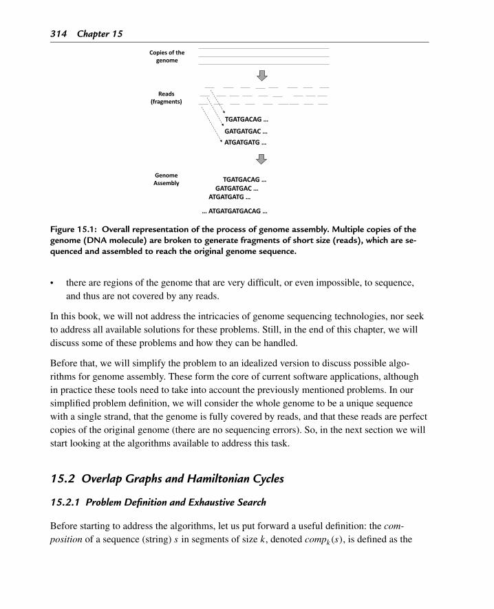
314 Chapter 15

Figure 15.1: Overall representation of the process of genome assembly. Multiple copies of thegenome (DNA molecule) are broken to generate fragments of short size (reads), which are se-quenced and assembled to reach the original genome sequence.

• there are regions of the genome that are very difficult, or even impossible, to sequence,and thus are not covered by any reads.

In this book, we will not address the intricacies of genome sequencing technologies, nor seekto address all available solutions for these problems. Still, in the end of this chapter, we willdiscuss some of these problems and how they can be handled.

Before that, we will simplify the problem to an idealized version to discuss possible algo-rithms for genome assembly. These form the core of current software applications, althoughin practice these tools need to take into account the previously mentioned problems. In oursimplified problem definition, we will consider the whole genome to be a unique sequencewith a single strand, that the genome is fully covered by reads, and that these reads are perfectcopies of the original genome (there are no sequencing errors). So, in the next section we willstart looking at the algorithms available to address this task.

15.2 Overlap Graphs and Hamiltonian Cycles

15.2.1 Problem Definition and Exhaustive Search

Before starting to address the algorithms, let us put forward a useful definition: the com-position of a sequence (string) s in segments of size k, denoted compk(s), is defined as the

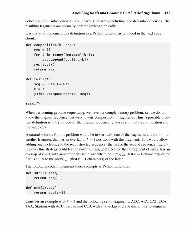
Assembling Reads Into Genomes: Graph-Based Algorithms 315

collection of all sub-sequences of s, of size k, possibly including repeated sub-sequences. Theresulting fragments are normally ordered lexicographically.

It is trivial to implement this definition as a Python function as provided in the next codechunk.

def composition(k, seq):res = []

f o r i in range( l e n (seq)−k+1):res.append(seq[i:i+k])

res.sort()

re turn res

def test1():seq = "CAATCATGATG"

k = 3

p r i n t (composition(k, seq))

test1()

When performing genome sequencing, we have the complementary problem, i.e. we do notknow the original sequence, but we know its composition in fragments. Thus, a possible prob-lem definition is to try to recover the original sequence, given as an input its composition andthe value of k.

A natural solution for this problem would be to start with one of the fragments and try to findanother fragment that has an overlap of k − 1 positions with this fragment. This would allowadding one nucleotide to the reconstructed sequence (the last of the second sequence). Iterat-ing over this strategy could lead to cover all fragments. Notice that a fragment of size k has anoverlap of k − 1 with another of the same size when the suffixk−1 (last k − 1 characters) of thefirst is equal to the prefixk−1 (first k − 1 characters) of the latter.

The following code implements these concepts as Python functions:

def suffix (seq):re turn seq[1:]

def prefix(seq):re turn seq[:−1]

Consider an example with k = 3 and the following set of fragments: ACC, ATA, CAT, CCA,TAA. Starting with ACC, we can find CCA with an overlap of 2 and this allows to augment

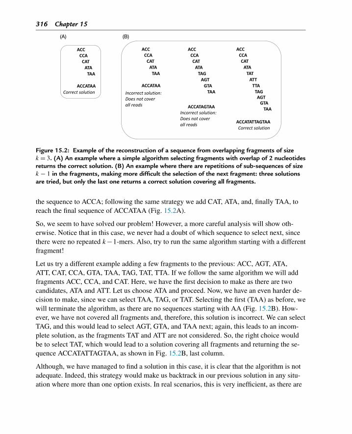
316 Chapter 15

Figure 15.2: Example of the reconstruction of a sequence from overlapping fragments of sizek = 3. (A) An example where a simple algorithm selecting fragments with overlap of 2 nucleotidesreturns the correct solution. (B) An example where there are repetitions of sub-sequences of sizek − 1 in the fragments, making more difficult the selection of the next fragment: three solutionsare tried, but only the last one returns a correct solution covering all fragments.

the sequence to ACCA; following the same strategy we add CAT, ATA, and, finally TAA, toreach the final sequence of ACCATAA (Fig. 15.2A).

So, we seem to have solved our problem! However, a more careful analysis will show oth-erwise. Notice that in this case, we never had a doubt of which sequence to select next, sincethere were no repeated k−1-mers. Also, try to run the same algorithm starting with a differentfragment!

Let us try a different example adding a few fragments to the previous: ACC, AGT, ATA,ATT, CAT, CCA, GTA, TAA, TAG, TAT, TTA. If we follow the same algorithm we will addfragments ACC, CCA, and CAT. Here, we have the first decision to make as there are twocandidates, ATA and ATT. Let us choose ATA and proceed. Now, we have an even harder de-cision to make, since we can select TAA, TAG, or TAT. Selecting the first (TAA) as before, wewill terminate the algorithm, as there are no sequences starting with AA (Fig. 15.2B). How-ever, we have not covered all fragments and, therefore, this solution is incorrect. We can selectTAG, and this would lead to select AGT, GTA, and TAA next; again, this leads to an incom-plete solution, as the fragments TAT and ATT are not considered. So, the right choice wouldbe to select TAT, which would lead to a solution covering all fragments and returning the se-quence ACCATATTAGTAA, as shown in Fig. 15.2B, last column.

Although, we have managed to find a solution in this case, it is clear that the algorithm is notadequate. Indeed, this strategy would make us backtrack in our previous solution in any situ-ation where more than one option exists. In real scenarios, this is very inefficient, as there are

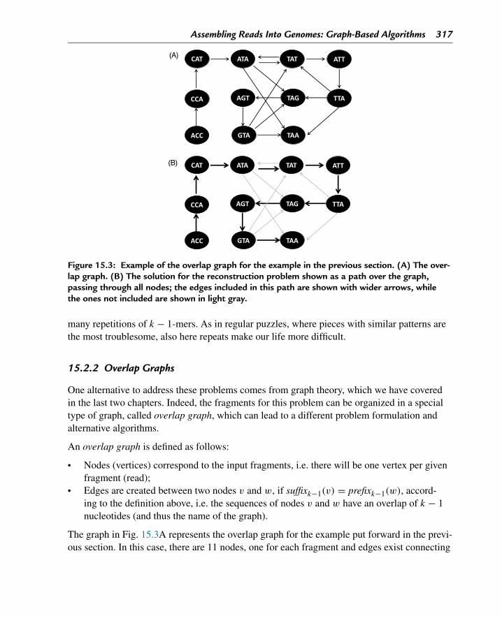
Assembling Reads Into Genomes: Graph-Based Algorithms 317

Figure 15.3: Example of the overlap graph for the example in the previous section. (A) The over-lap graph. (B) The solution for the reconstruction problem shown as a path over the graph,passing through all nodes; the edges included in this path are shown with wider arrows, whilethe ones not included are shown in light gray.

many repetitions of k − 1-mers. As in regular puzzles, where pieces with similar patterns arethe most troublesome, also here repeats make our life more difficult.

15.2.2 Overlap Graphs

One alternative to address these problems comes from graph theory, which we have coveredin the last two chapters. Indeed, the fragments for this problem can be organized in a specialtype of graph, called overlap graph, which can lead to a different problem formulation andalternative algorithms.

An overlap graph is defined as follows:

• Nodes (vertices) correspond to the input fragments, i.e. there will be one vertex per givenfragment (read);

• Edges are created between two nodes v and w, if suffixk−1(v) = prefixk−1(w), accord-ing to the definition above, i.e. the sequences of nodes v and w have an overlap of k − 1nucleotides (and thus the name of the graph).

The graph in Fig. 15.3A represents the overlap graph for the example put forward in the previ-ous section. In this case, there are 11 nodes, one for each fragment and edges exist connecting

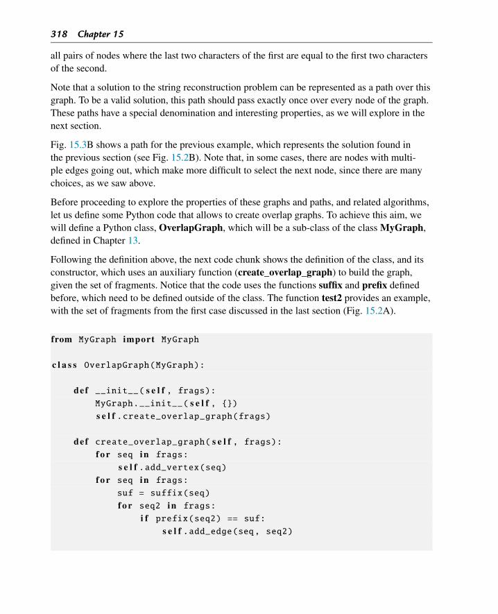
318 Chapter 15

all pairs of nodes where the last two characters of the first are equal to the first two charactersof the second.

Note that a solution to the string reconstruction problem can be represented as a path over thisgraph. To be a valid solution, this path should pass exactly once over every node of the graph.These paths have a special denomination and interesting properties, as we will explore in thenext section.

Fig. 15.3B shows a path for the previous example, which represents the solution found inthe previous section (see Fig. 15.2B). Note that, in some cases, there are nodes with multi-ple edges going out, which make more difficult to select the next node, since there are manychoices, as we saw above.

Before proceeding to explore the properties of these graphs and paths, and related algorithms,let us define some Python code that allows to create overlap graphs. To achieve this aim, wewill define a Python class, OverlapGraph, which will be a sub-class of the class MyGraph,defined in Chapter 13.

Following the definition above, the next code chunk shows the definition of the class, and itsconstructor, which uses an auxiliary function (create_overlap_graph) to build the graph,given the set of fragments. Notice that the code uses the functions suffix and prefix definedbefore, which need to be defined outside of the class. The function test2 provides an example,with the set of fragments from the first case discussed in the last section (Fig. 15.2A).

from MyGraph import MyGraph

c l a s s OverlapGraph(MyGraph):

def __init__( s e l f , frags):MyGraph.__init__( s e l f , {})s e l f .create_overlap_graph(frags)

def create_overlap_graph( s e l f , frags):f o r seq in frags:

s e l f .add_vertex(seq)f o r seq in frags:

suf = suffix(seq)

f o r seq2 in frags:

i f prefix(seq2) == suf:s e l f .add_edge(seq, seq2)

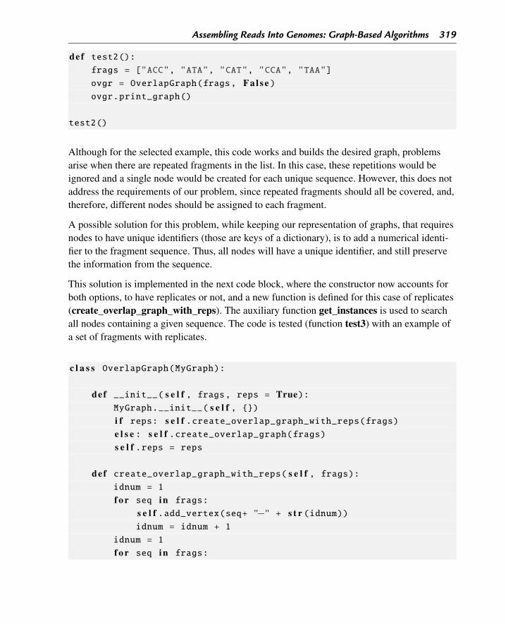
Assembling Reads Into Genomes: Graph-Based Algorithms 319

def test2():frags = ["ACC", "ATA", "CAT", "CCA", "TAA"]

ovgr = OverlapGraph(frags, F a l s e )ovgr.print_graph()

test2()

Although for the selected example, this code works and builds the desired graph, problemsarise when there are repeated fragments in the list. In this case, these repetitions would beignored and a single node would be created for each unique sequence. However, this does notaddress the requirements of our problem, since repeated fragments should all be covered, and,therefore, different nodes should be assigned to each fragment.

A possible solution for this problem, while keeping our representation of graphs, that requiresnodes to have unique identifiers (those are keys of a dictionary), is to add a numerical identi-fier to the fragment sequence. Thus, all nodes will have a unique identifier, and still preservethe information from the sequence.

This solution is implemented in the next code block, where the constructor now accounts forboth options, to have replicates or not, and a new function is defined for this case of replicates(create_overlap_graph_with_reps). The auxiliary function get_instances is used to searchall nodes containing a given sequence. The code is tested (function test3) with an example ofa set of fragments with replicates.

c l a s s OverlapGraph(MyGraph):

def __init__( s e l f , frags, reps = True):MyGraph.__init__( s e l f , {})i f reps: s e l f .create_overlap_graph_with_reps(frags)e l s e : s e l f .create_overlap_graph(frags)s e l f .reps = reps

def create_overlap_graph_with_reps( s e l f , frags):idnum = 1

f o r seq in frags:

s e l f .add_vertex(seq+ "−" + s t r (idnum))idnum = idnum + 1

idnum = 1

f o r seq in frags:

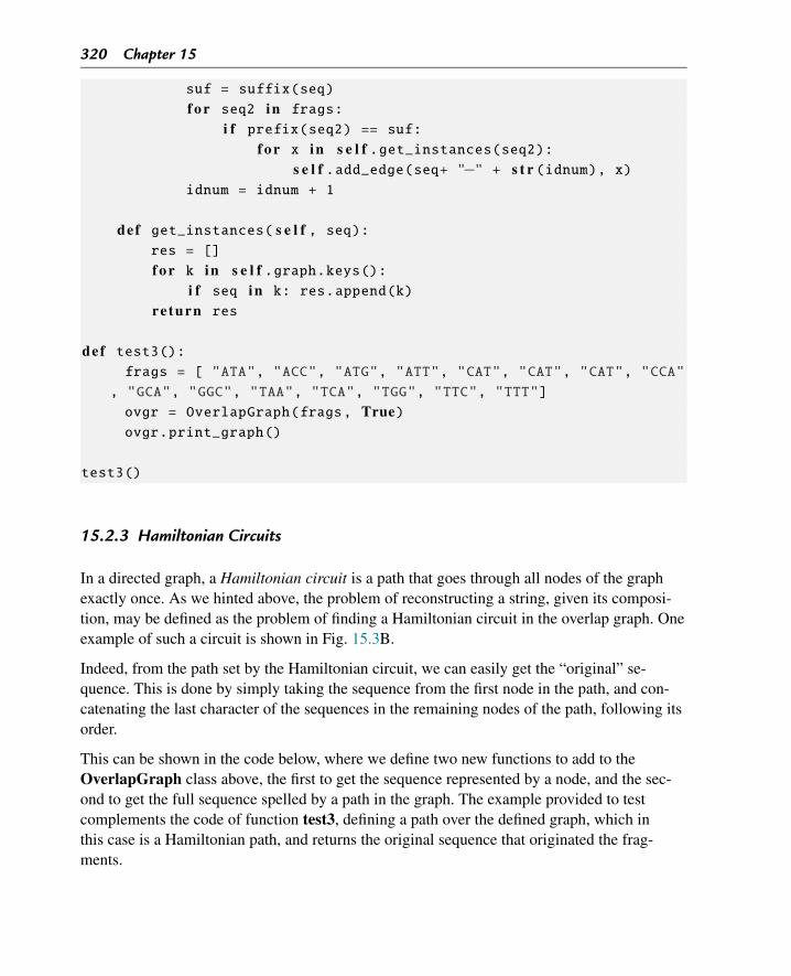
320 Chapter 15

suf = suffix(seq)

f o r seq2 in frags:

i f prefix(seq2) == suf:f o r x in s e l f .get_instances(seq2):

s e l f .add_edge(seq+ "−" + s t r (idnum), x)idnum = idnum + 1

def get_instances( s e l f , seq):res = []

f o r k in s e l f .graph.keys():i f seq in k: res.append(k)

re turn res

def test3():frags = [ "ATA", "ACC", "ATG", "ATT", "CAT", "CAT", "CAT", "CCA"

, "GCA", "GGC", "TAA", "TCA", "TGG", "TTC", "TTT"]

ovgr = OverlapGraph(frags, True)ovgr.print_graph()

test3()

15.2.3 Hamiltonian Circuits

In a directed graph, a Hamiltonian circuit is a path that goes through all nodes of the graphexactly once. As we hinted above, the problem of reconstructing a string, given its composi-tion, may be defined as the problem of finding a Hamiltonian circuit in the overlap graph. Oneexample of such a circuit is shown in Fig. 15.3B.

Indeed, from the path set by the Hamiltonian circuit, we can easily get the “original” se-quence. This is done by simply taking the sequence from the first node in the path, and con-catenating the last character of the sequences in the remaining nodes of the path, following itsorder.

This can be shown in the code below, where we define two new functions to add to theOverlapGraph class above, the first to get the sequence represented by a node, and the sec-ond to get the full sequence spelled by a path in the graph. The example provided to testcomplements the code of function test3, defining a path over the defined graph, which inthis case is a Hamiltonian path, and returns the original sequence that originated the frag-ments.

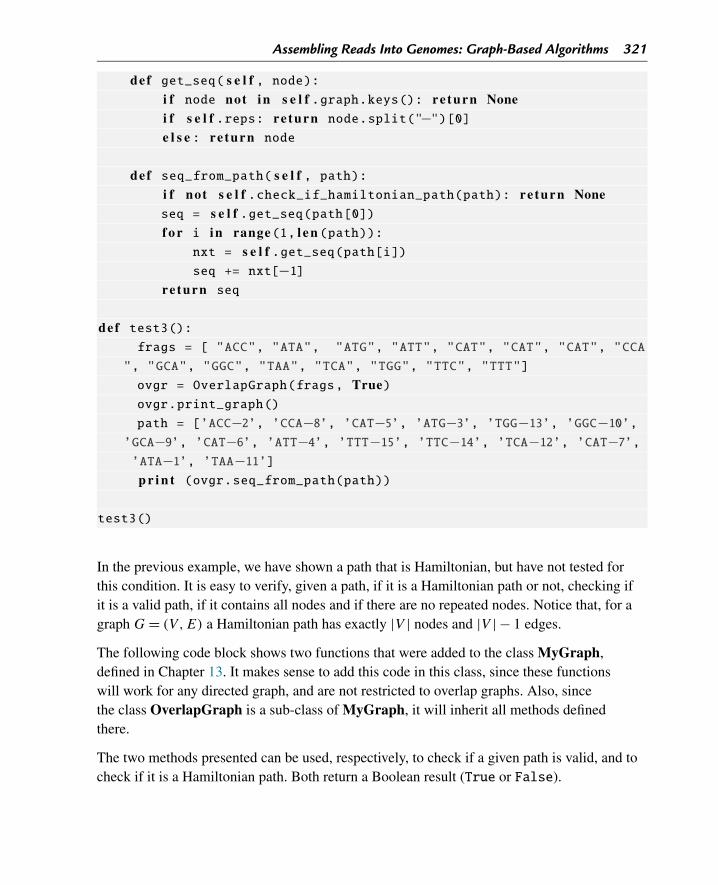
Assembling Reads Into Genomes: Graph-Based Algorithms 321

def get_seq( s e l f , node):i f node not in s e l f .graph.keys(): re turn Nonei f s e l f .reps: re turn node.split("−")[0]e l s e : re turn node

def seq_from_path( s e l f , path):i f not s e l f .check_if_hamiltonian_path(path): re turn Noneseq = s e l f .get_seq(path[0])f o r i in range(1, l e n (path)):

nxt = s e l f .get_seq(path[i])seq += nxt[−1]

re turn seq

def test3():frags = [ "ACC", "ATA", "ATG", "ATT", "CAT", "CAT", "CAT", "CCA

", "GCA", "GGC", "TAA", "TCA", "TGG", "TTC", "TTT"]

ovgr = OverlapGraph(frags, True)ovgr.print_graph()

path = [’ACC−2’, ’CCA−8’, ’CAT−5’, ’ATG−3’, ’TGG−13’, ’GGC−10’,’GCA−9’, ’CAT−6’, ’ATT−4’, ’TTT−15’, ’TTC−14’, ’TCA−12’, ’CAT−7’,’ATA−1’, ’TAA−11’]p r i n t (ovgr.seq_from_path(path))

test3()

In the previous example, we have shown a path that is Hamiltonian, but have not tested forthis condition. It is easy to verify, given a path, if it is a Hamiltonian path or not, checking ifit is a valid path, if it contains all nodes and if there are no repeated nodes. Notice that, for agraph G = (V ,E) a Hamiltonian path has exactly |V | nodes and |V | − 1 edges.

The following code block shows two functions that were added to the class MyGraph,defined in Chapter 13. It makes sense to add this code in this class, since these functionswill work for any directed graph, and are not restricted to overlap graphs. Also, sincethe class OverlapGraph is a sub-class of MyGraph, it will inherit all methods definedthere.

The two methods presented can be used, respectively, to check if a given path is valid, and tocheck if it is a Hamiltonian path. Both return a Boolean result (True or False).

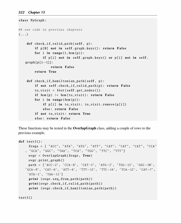
322 Chapter 15

c l a s s MyGraph:

## see code in previous chapters

(...)

def check_if_valid_path( s e l f , p):i f p[0] not in s e l f .graph.keys(): re turn F a l s ef o r i in range(1, l e n (p)):

i f p[i] not in s e l f .graph.keys() or p[i] not in s e l f .graph[p[i−1]]:

re turn F a l s ere turn True

def check_if_hamiltonian_path( s e l f , p):i f not s e l f .check_if_valid_path(p): re turn F a l s eto_visit = l i s t ( s e l f .get_nodes())i f l e n (p) != l e n (to_visit): re turn F a l s ef o r i in range( l e n (p)):

i f p[i] in to_visit: to_visit.remove(p[i])

e l s e : re turn F a l s ei f not to_visit: re turn Truee l s e : re turn F a l s e

These functions may be tested in the OverlapGraph class, adding a couple of rows to theprevious example.

def test3():frags = [ "ACC", "ATA", "ATG", "ATT", "CAT", "CAT", "CAT", "CCA"

, "GCA", "GGC", "TAA", "TCA", "TGG", "TTC", "TTT"]

ovgr = OverlapGraph(frags, True)ovgr.print_graph()

path = [’ACC−2’, ’CCA−8’, ’CAT−5’, ’ATG−3’, ’TGG−13’, ’GGC−10’,’GCA−9’, ’CAT−6’, ’ATT−4’, ’TTT−15’, ’TTC−14’, ’TCA−12’, ’CAT−7’,’ATA−1’, ’TAA−11’]p r i n t (ovgr.seq_from_path(path))p r i n t (ovgr.check_if_valid_path(path))p r i n t (ovgr.check_if_hamiltonian_path(path))

test3()

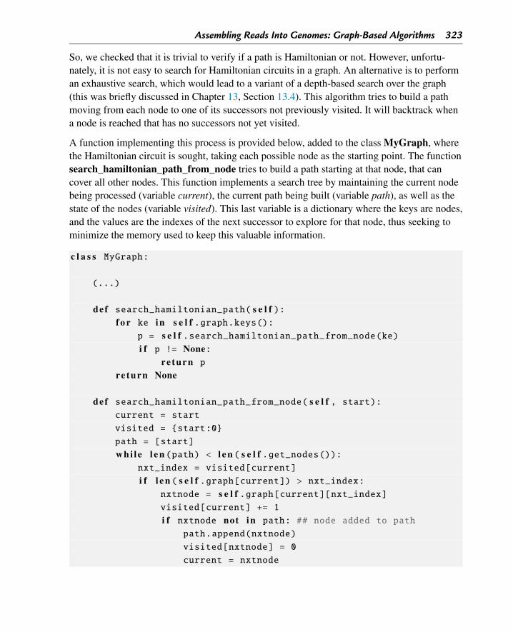
Assembling Reads Into Genomes: Graph-Based Algorithms 323

So, we checked that it is trivial to verify if a path is Hamiltonian or not. However, unfortu-nately, it is not easy to search for Hamiltonian circuits in a graph. An alternative is to performan exhaustive search, which would lead to a variant of a depth-based search over the graph(this was briefly discussed in Chapter 13, Section 13.4). This algorithm tries to build a pathmoving from each node to one of its successors not previously visited. It will backtrack whena node is reached that has no successors not yet visited.

A function implementing this process is provided below, added to the class MyGraph, wherethe Hamiltonian circuit is sought, taking each possible node as the starting point. The functionsearch_hamiltonian_path_from_node tries to build a path starting at that node, that cancover all other nodes. This function implements a search tree by maintaining the current nodebeing processed (variable current), the current path being built (variable path), as well as thestate of the nodes (variable visited). This last variable is a dictionary where the keys are nodes,and the values are the indexes of the next successor to explore for that node, thus seeking tominimize the memory used to keep this valuable information.

c l a s s MyGraph:

(...)

def search_hamiltonian_path( s e l f ):f o r ke in s e l f .graph.keys():

p = s e l f .search_hamiltonian_path_from_node(ke)i f p != None:

re turn pre turn None

def search_hamiltonian_path_from_node( s e l f , start):current = start

visited = {start:0}

path = [start]

whi le l e n (path) < l e n ( s e l f .get_nodes()):nxt_index = visited[current]

i f l e n ( s e l f .graph[current]) > nxt_index:nxtnode = s e l f .graph[current][nxt_index]visited[current] += 1

i f nxtnode not in path: ## node added to path

path.append(nxtnode)

visited[nxtnode] = 0

current = nxtnode

324 Chapter 15

e l s e : ## backtracki f l e n (path) > 1:

rmvnode = path.pop()

d e l visited[rmvnode]current = path[−1]

e l s e : re turn Nonereturn path

The previous function can be tested in the context of the OverlapGraph class, in the previousexamples, as shown below.

def test4():frags = [ "ACC", "ATA", "ATG", "ATT", "CAT", "CAT", "CAT", "CCA",

"GCA", "GGC", "TAA", "TCA", "TGG", "TTC", "TTT"]

ovgr = OverlapGraph(frags, True)ovgr.print_graph()

path = ovgr.search_hamiltonian_path()

p r i n t (path)p r i n t (ovgr.check_if_hamiltonian_path(path))p r i n t (ovgr.seq_from_path(path))

test4()

We can now close the circle by defining a sequence, calculating its composition and trying torecover it by finding a Hamiltonian circuit. This is done in the next example.

def test5():orig_sequence = "CAATCATGATGATGATC"

frags = composition(3, orig_sequence)

p r i n t (frags)ovgr = OverlapGraph(frags, True)ovgr.print_graph()

path = ovgr.search_hamiltonian_path()

p r i n t (path)p r i n t (ovgr.seq_from_path(path))

test5()

However, as the reader can check by running the example, the recovered sequence is not thesame. This happens since there might be many different sequences with the same composi-tion. This becomes increasingly rarer as the value of k becomes larger.

Assembling Reads Into Genomes: Graph-Based Algorithms 325

Also, we invite the reader to try to increase the size of the sequence and check that the algo-rithm starts to behave increasingly worse in terms of its run time. In fact, this algorithm cannot be used for large sequences, and respective overlap graphs. Indeed, the problem of findingHamiltonian graphs is quite complex, belonging to the class of NP-hard optimization prob-lems, which implies that no efficient algorithms exist when the problem scales, in this case,when the graph becomes larger.

This makes it very difficult, in practice, to use this approach for large-scale genome assembly.Still, until a few years ago, these were the strategies used by the existing programs, whichused heuristic methods to attain the best possible solutions. These were used, for instance,throughout the Human Genome Project.

15.3 DeBruijn Graphs and Eulerian Paths

15.3.1 DeBruijn Graphs for Genome Assembly

Given that the previous attempt to represent the problem data, using overlap graphs, was notsuccessful in finding efficient algorithms, other solutions were sought by the research commu-nity. Indeed, approaching similar problems, while at the time not related to genome assembly,the mathematician DeBruijn proposed a distinct representation, which also makes use of di-rected graphs.

The idea is to represent the fragments of the problem as edges, and not as vertices. Here, thesolutions to the problem would, therefore, be paths over the graph containing all edges exactlyonce. We will explore this in further detail in the next section.

In the case of DeBruijn graphs, the nodes contain sequences that correspond to either aprefixk−1 or a suffixk−1 of one of the fragments. So, each edge, corresponding to a fragment,connects a node representing its prefixk−1 to a node representing its suffixk−1. In this case, un-like in the previous overlap graphs, prefixes and suffixes of length k − 1, which share the samesequence, are represented in a single node. So, repeated fragments are represented as multipleedges connecting the same pair of nodes. Fig. 15.4 shows the representation of the examplefrom the previous section, the one implemented in the functions test3 and test4 above, as aDeBruijn graph. The set of 15 fragments is ACC, ATA, ATG, ATT, CAT, CAT, CAT, CCA,GCA, GGC, TAA, TCA, TGG, TTC, and TTT. Thus, the graph has 15 edges and 11 uniquek − 1-mers that are either prefixes or suffixes (or both) of these fragments.

As before, we will here implement DeBruijn graphs as a Python class, DeBruijnGraph,that also extends the class MyGraph. In this case, this class needs to redefine the functionadd_adge to allow repeated edges between the same pair of nodes. The function create_

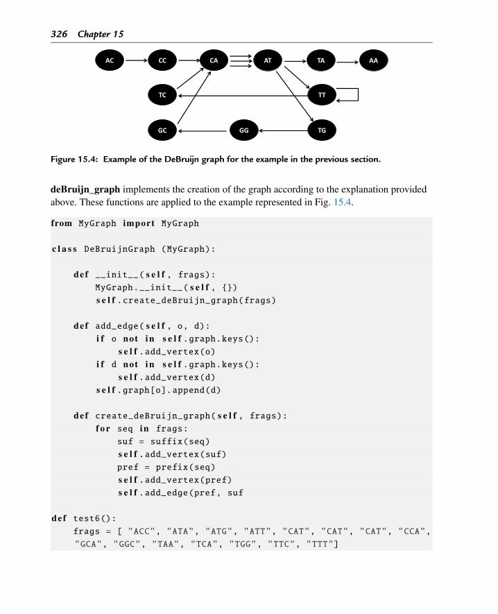
326 Chapter 15

Figure 15.4: Example of the DeBruijn graph for the example in the previous section.

deBruijn_graph implements the creation of the graph according to the explanation providedabove. These functions are applied to the example represented in Fig. 15.4.

from MyGraph import MyGraph

c l a s s DeBruijnGraph (MyGraph):

def __init__( s e l f , frags):MyGraph.__init__( s e l f , {})s e l f .create_deBruijn_graph(frags)

def add_edge( s e l f , o, d):i f o not in s e l f .graph.keys():

s e l f .add_vertex(o)i f d not in s e l f .graph.keys():

s e l f .add_vertex(d)s e l f .graph[o].append(d)

def create_deBruijn_graph( s e l f , frags):f o r seq in frags:

suf = suffix(seq)

s e l f .add_vertex(suf)pref = prefix(seq)

s e l f .add_vertex(pref)s e l f .add_edge(pref, suf

def test6():frags = [ "ACC", "ATA", "ATG", "ATT", "CAT", "CAT", "CAT", "CCA",

"GCA", "GGC", "TAA", "TCA", "TGG", "TTC", "TTT"]

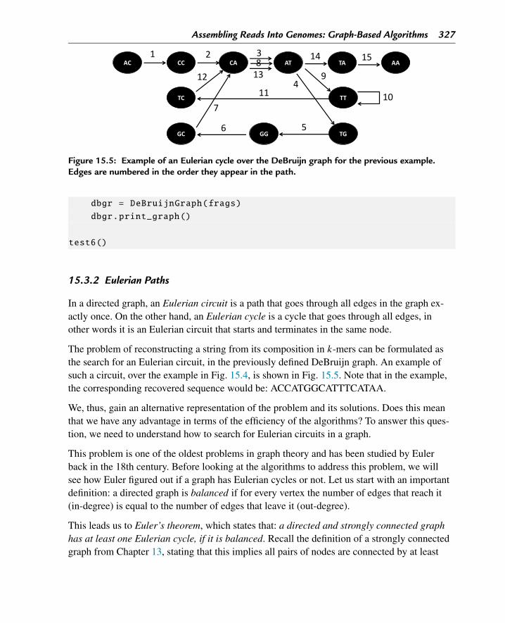
Assembling Reads Into Genomes: Graph-Based Algorithms 327

Figure 15.5: Example of an Eulerian cycle over the DeBruijn graph for the previous example.Edges are numbered in the order they appear in the path.

dbgr = DeBruijnGraph(frags)

dbgr.print_graph()

test6()

15.3.2 Eulerian Paths

In a directed graph, an Eulerian circuit is a path that goes through all edges in the graph ex-actly once. On the other hand, an Eulerian cycle is a cycle that goes through all edges, inother words it is an Eulerian circuit that starts and terminates in the same node.

The problem of reconstructing a string from its composition in k-mers can be formulated asthe search for an Eulerian circuit, in the previously defined DeBruijn graph. An example ofsuch a circuit, over the example in Fig. 15.4, is shown in Fig. 15.5. Note that in the example,the corresponding recovered sequence would be: ACCATGGCATTTCATAA.

We, thus, gain an alternative representation of the problem and its solutions. Does this meanthat we have any advantage in terms of the efficiency of the algorithms? To answer this ques-tion, we need to understand how to search for Eulerian circuits in a graph.

This problem is one of the oldest problems in graph theory and has been studied by Eulerback in the 18th century. Before looking at the algorithms to address this problem, we willsee how Euler figured out if a graph has Eulerian cycles or not. Let us start with an importantdefinition: a directed graph is balanced if for every vertex the number of edges that reach it(in-degree) is equal to the number of edges that leave it (out-degree).

This leads us to Euler’s theorem, which states that: a directed and strongly connected graphhas at least one Eulerian cycle, if it is balanced. Recall the definition of a strongly connectedgraph from Chapter 13, stating that this implies all pairs of nodes are connected by at least

328 Chapter 15

one path. This theorem provides an easy way to check if the graph has an Eulerian cycle ornot.

We have seen previously that a solution for our problem is represented by an Eulerian cir-cuit, but the previous theorem states the conditions for the existence of an Eulerian cycle. Thedifference is subtle but important. Indeed, an extension of the previous theorem states thata directed strongly connected graph has an Eulerian circuit if it is nearly balanced, whichmeans it contains, at most, two semi-balanced vertices (i.e. whose difference between the inand the out-degree is −1 and 1, respectively), while all other vertices are balanced.

These definitions can be implemented in Python, by creating functions within the context ofthe class MyGraph, that check if graphs are balanced or semi-balanced. Note that a func-tion to test if a graph is strongly connected was previously defined in Chapter 13. The firstfunction checks if a node is balanced, the second if a graph is balanced (i.e. all nodes are bal-anced), and the third if the graph is nearly balanced, according to the definitions above.

def check_balanced_node( s e l f , node):re turn s e l f .in_degree(node) == s e l f .out_degree(node)

def check_balanced_graph( s e l f ):f o r n in s e l f .graph.keys():

i f not s e l f .check_balanced_node(n): re turn F a l s ere turn True

def check_nearly_balanced_graph( s e l f ):res = None, Nonef o r n in s e l f .graph.keys():

indeg= s e l f .in_degree(n)outdeg= s e l f .out_degree(n)i f indeg − outdeg == 1 and res[1] i s None: res = res[0],

n

e l i f indeg − outdeg == −1 and res[0] i s None: res = n,res[1]

e l i f indeg == outdeg: passe l s e : re turn None, None

return res

Note that to apply the previous functions to DeBruijn graphs, i.e. in the context of the Pythonclass DeBruijnGraph, we need to redefine the way the in-degree is calculated, to account forpossible multiple edges with the same origin and successor in these graphs.

Assembling Reads Into Genomes: Graph-Based Algorithms 329

c l a s s DeBruijnGraph (MyGraph):

(...)

def in_degree( s e l f , v):res = 0

f o r k in s e l f .graph.keys():i f v in s e l f .graph[k]:

res += s e l f .graph[k].count(v)re turn res

The next step is to design an algorithm to search for Eulerian cycles, for graphs that containat least one. This algorithm is quite straightforward, and can be summarized in the followingsteps:

1. We start by any vertex v in the graph and choose one of its successors; we continue thisprocess always selecting from each node a successor that uses a non-visited edge. Asthe graph is balanced and connected, we will always reach v after a given number ofsteps.

2. If the cycle in the previous step is not yet an Eulerian cycle, i.e. it still does not containall edges, we need to select a vertex w from the path in step 1 with non-visited edges. Werepeat step 1 starting in w, until reaching w again.

3. The cycles from steps 1 and 2 can be combined, by going from v to w (part of the firstcycle), doing the cycle in the second step and returning to w, and going from w to v (lastpart of the first cycle).

4. While an Eulerian cycle is not attained, go back to step 2, select a vertex w from the cur-rent cycle and perform the steps 2 and 3.

Fig. 15.6 shows an example of the application of the previous algorithm for a given graph. Inthis case, the first selected node is a, and step 1 gathers the cycle going through nodes a, d, g,h, a. Since this is not an Eulerian cycle, we need to select a node with non-visited edges, andselect g. In step 2, thus we build the cycle g, f, e, c, g, that in step 3 can be combined with theprevious to get a cycle doing a, d, g, f, e, c, g, h, a. Since this is still not an Eulerian cycle, wereturn to step 2 select another node with non-visited edges, in this case c, getting the cycle c,a, b, c. We, finally, join this cycle with the previous to get a, d, g, f, e, c, a, b, c, g, h, a, whichis now an Eulerian cycle (Fig. 15.6B).

This algorithm can be implemented within the class MyGraph to find Eulerian cycles asshown in the function below.

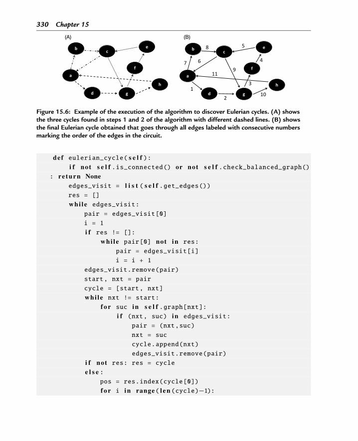
330 Chapter 15

Figure 15.6: Example of the execution of the algorithm to discover Eulerian cycles. (A) showsthe three cycles found in steps 1 and 2 of the algorithm with different dashed lines. (B) showsthe final Eulerian cycle obtained that goes through all edges labeled with consecutive numbersmarking the order of the edges in the circuit.

def eulerian_cycle( s e l f ):i f not s e l f .is_connected() or not s e l f .check_balanced_graph()

: re turn Noneedges_visit = l i s t ( s e l f .get_edges())res = []

whi le edges_visit:pair = edges_visit[0]

i = 1

i f res != []:whi le pair[0] not in res:

pair = edges_visit[i]

i = i + 1

edges_visit.remove(pair)

start, nxt = pair

cycle = [start, nxt]

whi le nxt != start:f o r suc in s e l f .graph[nxt]:

i f (nxt, suc) in edges_visit:

pair = (nxt,suc)

nxt = suc

cycle.append(nxt)

edges_visit.remove(pair)

i f not res: res = cyclee l s e :

pos = res.index(cycle[0])

f o r i in range( l e n (cycle)−1):

Assembling Reads Into Genomes: Graph-Based Algorithms 331

res.insert(pos + i +1, cycle[i+1])

re turn res

To be useful in our context, however, we need to compute Eulerian circuits and not cycles. Aswe saw above, the difference can be addressed with minor effort. Indeed, we can transforma nearly balanced graph into a balanced one by adding an edge connecting the two semi-balanced nodes to make them balanced. If we calculate an Eulerian cycle for this “extended”graph, removing this extra edge will lead to an Eulerian circuit of the original graph.

This idea is implemented in the next function, again added to the class MyGraph.

def eulerian_path( s e l f ):unb = s e l f .check_nearly_balanced_graph()i f unb[0] i s None or unb[1] i s None: re turn Nones e l f .graph[unb[1]].append(unb[0])cycle = s e l f .eulerian_cycle()f o r i in range( l e n (cycle)−1):

i f cycle[i] == unb[1] and cycle[i+1] == unb[0]:

breakpath = cycle[i+1:] + cycle[1:i+1]

re turn path

These functions may be tested within the DeBruijnGraph class, considering the previousexample, as shown below. Notice that the Eulerian path computed in function test6 is the oneprovided in Fig. 15.5.

c l a s s DeBruijnGraph (MyGraph):

(...) # code above for this class

def seq_from_path( s e l f , path):seq = path[0]

f o r i in range(1, l e n (path)):nxt = path[i]

seq += nxt[−1]re turn seq

def test6():frags = [ "ATA", "ACC", "ATG", "ATT", "CAT", "CAT", "CAT", "CCA",

"GCA", "GGC", "TAA", "TCA", "TGG", "TTC", "TTT"]

332 Chapter 15

dbgr = DeBruijnGraph(frags)

dbgr.print_graph()

p r i n t (dbgr.is_connected())p r i n t (dbgr.check_nearly_balanced_graph())p r i n t (dbgr.eulerian_path())

def test7():orig_sequence = "ATGCAATGGTCTG"

frags = composition(3, orig_sequence)

dbgr = DeBruijnGraph(frags)

dbgr.print_graph()

p r i n t (dbgr.check_nearly_balanced_graph())p= dbgr.eulerian_path()

p r i n t (p)p r i n t (dbgr.seq_from_path(p))

test6()

test7()

The last example shows the closing of the cycle as in the previous section, i.e. we start with asequence, calculate its composition and try to recover the original sequence.

Fortunately, as you may hint for the above algorithms, this problem has a much lower com-plexity, when compared to the search for Hamiltonian cycles. Indeed, the above algorithmcan be implemented quite efficiently and can be run for large graphs without a problem. Thus,most of the recent genome assembly programs implement this strategy at their core, as wewill discuss in the next section.

15.4 Genome Assembly in Practice

In this section, we will cover a number of issues related to genome assembly in the real world,which complicate the life of the software developers in this field, far beyond the idealizedversions of the problem considered in previous sections.

One of the main problems in assembling genomes from real reads is the read length. Indeed,the larger this value is the easier it is to assemble genomes, as the DeBruijn graphs tend tobecome linear (with a single path). However, current technologies are still limited in the readlengths they provide. Another related problem is the assignment of reads to one of the twostrands.

Assembling Reads Into Genomes: Graph-Based Algorithms 333

Paired-end reads, a commonly used feature in recent technologies help to alleviate these prob-lems. They provide larger read lengths and help to disambiguate the strand. In this case, pairsof reads, with a relatively fixed distance in the genome between themselves, are generated.Thus, each read will be a pair of sequences of length l (being l the read length). The previousalgorithms based on DeBruijn graphs can be generalized to accommodate paired end reads,but the details of these algorithms will not be covered here.

Another practical problem, when reconstructing genomes from reads (fragments) is the non-perfect coverage. Depending on the technology and the genome characteristics there will beparts of the original sequence that are not captured by the sequencing reads. A solution is toselect a value of k smaller than the original read length l, and replace the original reads byall possible reads of size k contained in the original ones, i.e. all sub-strings of size k of theoriginal string of size l. These new “reads” will then be used as an input to the previous algo-rithms.

A common problem with real-world assembly is the fact that all technologies produce errorsin the reads. In some of the technologies the errors can account to 1 to 5% of the read length.In the DeBruijn graphs, if we insert a read with an error this will cause an alternative path tobe created in the graph, in a structure normally called a bubble. Modern assembly softwaretools attempt to find and remove these bubbles from the graph, while performing the assem-bly. In this case, they need to be able to identify real bubbles, without removing correct paths,which may be a complex task in areas with repeats with some variation.

Depending on the species, the genome may contain many repeated regions, which can be asmuch as 50% of the entire genome. This represents a very hard problem for assembly pro-grams. Moreover, genomes contain copy-number alterations, i.e. large blocks of sequencethat are repeated multiple times. Assembly programs can estimate the number of copies bydetermining how the coverage in these regions deviate from the expected coverage or by com-paring with other regions of the genomes.

Given all these natural and technical problems, even the most sophisticated software toolsavailable have difficulties in generating a single sequence from a set of reads, and in mostcases generate a set of contigs, the sequences generated from paths in parts (non-branching)of the DeBruijn graph. In many real cases, it is common to end up with hundreds or eventhousands of contigs, even when assembling the genomes of simple organisms, as bacteria.In order to assess the quality of an assembly one of the most commonly used measures is theN50. It is a measure of contiguity derived from the length of the assembled contigs, similarto the median of the lengths. The contigs are sorted by their increasing length and the N50corresponds to the length of the shortest contig at 50% of the summed assembled genome.

The order of the contigs is not known from the result of these algorithms. The process oftaking the contigs, ordering them and trying to close possible gaps, to reach a final single

334 Chapter 15

genome, is typically quite costly as it involves a lot of manual curation, and may be impos-sible to achieve. One alternative is to sequence the same genome using different technologiesand try to combine their results to make this process easier.

Still, and in spite of all these difficulties, DeBruijn graphs are the basis of most efficient mod-ern assembly software tools able to handle large datasets with many millions of reads. TheVelvet algorithm [158] was of major importance in the field. Not only it is an efficient al-gorithm but it was also the starting point of further developments that include: IDBA [124],SPAdes [20], SOAPdenovo2 [104] or Megahit [99]. Comparison studies show that DeBruijngraph-based assemblers have a very competitive performance when handling very largedatasets, with relatively longer read lengths (75bps) requiring shorter runtime and main mem-ory requirements [160]. All the previous alternatives need to face the problems described inthis section (and others), and most of the recent advances in the field are related to improve-ments in the way they handle these challenges.

Bibliographic Notes and Further Reading

Euler’s pioneer work on graph theory and Eulerian cycles was described in [60]. DeBruijngraphs were introduced by Nicolaas De Bruijn in [44]. The algorithm for Eulerian cyclesearching was developed by Hierholzer in 1873 [76]. The Eulerian approach to genome as-sembly was first proposed in 1995 by Idury and Waterman [80], and improved in a study byPevzner et al. in 2001 [127]. The approaches based on DeBruijn graphs for paired end readswere proposed by Medvedev et al. [110], being covered, for instance, in [35] (Chapter 3).

Exercises and Programming Projects

Exercises

1. Consider the algorithm (and its implementation) that allows the determination of Euleriancycles of a graph. Write a version of this function that can handle non-connected graphs(still balanced). This function should allow to calculate all Eulerian cycles of the differentconnected components.

2. One of the problems when reconstructing genomes from reads (fragments) is the non-perfect coverage, as we saw above in Section 15.4. Write a function that has as its inputsthe original set of fragments, and returns the original sequence that generated the frag-ments, using DeBruijn graphs, following the strategy explained above. You should test allvalues of k starting by the read length, and decrement k by 1, until a value of k allows toreach a graph with an Eulerian circuit. If it does not work for k = 2, the function shouldreturn None.

Assembling Reads Into Genomes: Graph-Based Algorithms 335

3. Write a method to add to the class DeBruijnGraph that given the graph (self ) identifiesthe connected components of the graph (notice that in a directed graph, a connected com-ponent is a sub-graph that includes a set of nodes that are strongly connected among eachother, i.e. there are paths connecting all pairs of nodes), selects the largest one (if it ex-ists) and re-builds the sequence from the graph. If there are no connected components inthe graph, the methods should return None.

Programming Projects

1. Implement algorithms based on DeBruijn graphs to be able to work with paired endreads.

CHAPTER 16

Matching Reads to Reference SequencesThe problem of pattern finding over target sequences will be revisited in this chapter, lookingat scenarios where we have a set of sub-strings to be searched over a large sequence. This hasimportant applications in the processing of DNA sequencing data, when a set of reads/frag-ments needs to be searched over a full reference genome. We will mainly focus on algorithmsand data structures that allow to pre-process the reference sequence, making more efficient tosearch distinct patterns, also addressing methods to reduce the memory requirements.

16.1 Introduction: Problem Definition and ApplicationsIn this chapter, we will address a common problem in today’s Bioinformatics, namely in han-dling DNA/RNA sequencing data. In many cases, we are faced with the need to find a largeset of sequences, typically smaller sequences up to a few hundred nucleotides representingreads from a sequencing project, in a large reference sequence, such as a full genome or achromosome.

In Chapter 5, we have discussed the problem of finding a fixed pattern (sub-string) in a targetsequence and discussed several ways to improve the performance of the respective algo-rithms, for instance by suitable pre-processing of the pattern to search. This made the searchof a single pattern in a set of sequences more efficient. In this case, we want to search a setof different patterns over the same target sequence, a feature that changes the context of theproblem.

In the next section, we will start by looking at tries a structure that allows to pre-process aset of patterns. We will then move to study a similar structure, suffix trees, that allows to pre-process the target sequence, making the search over it more efficient. Finally, we will look atBurrows-Wheeler transforms as a way to further improve the memory needed to keep refer-ence sequences, which are important when the target sequences are very large, as it is the casewith full genomes.

16.2 Pre-Processing the Patterns: Tries16.2.1 Definitions and Algorithms

Tries are n-ary trees that allow to organize a set of string patterns. We have addressed the con-cept of trees in Chapter 9, while we mostly discussed binary trees. In the case of tries, eachinternal node can have n branches (with n ≥ 1).

Bioinformatics Algorithms. DOI: 10.1016/B978-0-12-812520-5.00016-XCopyright © 2018 Elsevier Inc. All rights reserved. 337

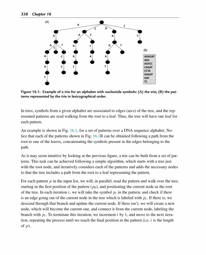
338 Chapter 16

Figure 16.1: Example of a trie for an alphabet with nucleotide symbols: (A) the trie; (B) the pat-terns represented by the trie in lexicographical order.

In tries, symbols from a given alphabet are associated to edges (arcs) of the tree, and the rep-resented patterns are read walking from the root to a leaf. Thus, the tree will have one leaf foreach pattern.

An example is shown in Fig. 16.1, for a set of patterns over a DNA sequence alphabet. No-tice that each of the patterns shown in Fig. 16.1B can be obtained following a path from theroot to one of the leaves, concatenating the symbols present in the edges belonging to thepath.

As it may seem intuitive by looking at the previous figure, a trie can be built from a set of pat-terns. This task can be achieved following a simple algorithm, which starts with a tree justwith the root node, and iteratively considers each of the patterns and adds the necessary nodesto that the tree includes a path from the root to a leaf representing the pattern.

For each pattern p in the input list, we will, in parallel, read the pattern and walk over the tree,starting in the first position of the pattern (p0), and positioning the current node as the rootof the tree. In each iteration i, we will take the symbol pi in the pattern, and check if thereis an edge going out of the current node in the tree which is labeled with pi . If there is, wedescend through that branch and update the current node. If there isn’t, we will create a newnode, which will become the current one, and connect it from the current node, labeling thebranch with pi . To terminate this iteration, we increment i by 1, and move to the next itera-tion, repeating the process until we reach the final position in the pattern (i.e. i is the lengthof p).

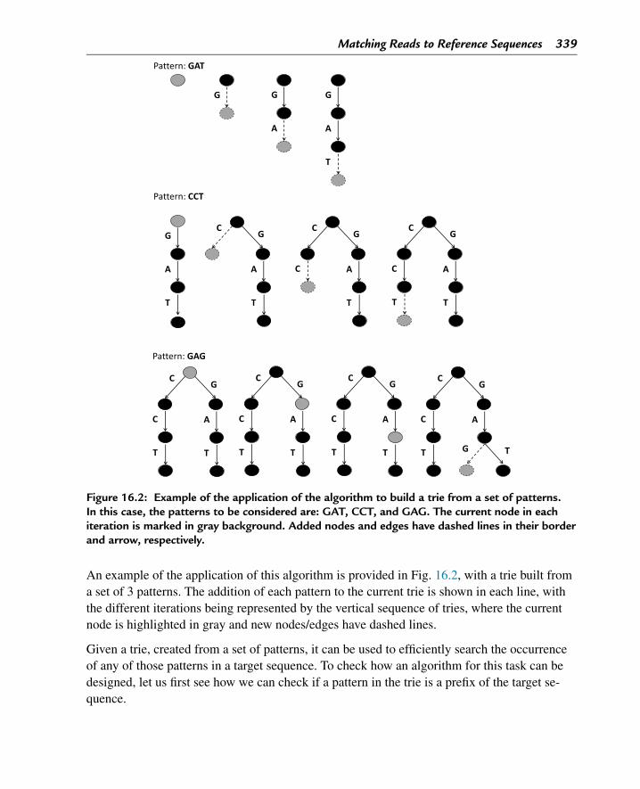
Matching Reads to Reference Sequences 339

Figure 16.2: Example of the application of the algorithm to build a trie from a set of patterns.In this case, the patterns to be considered are: GAT, CCT, and GAG. The current node in eachiteration is marked in gray background. Added nodes and edges have dashed lines in their borderand arrow, respectively.

An example of the application of this algorithm is provided in Fig. 16.2, with a trie built froma set of 3 patterns. The addition of each pattern to the current trie is shown in each line, withthe different iterations being represented by the vertical sequence of tries, where the currentnode is highlighted in gray and new nodes/edges have dashed lines.

Given a trie, created from a set of patterns, it can be used to efficiently search the occurrenceof any of those patterns in a target sequence. To check how an algorithm for this task can bedesigned, let us first see how we can check if a pattern in the trie is a prefix of the target se-quence.

340 Chapter 16

In this case, we just go through the characters in the sequence and in parallel walk over thetrie, starting in the root, following the edges corresponding to the characters in the sequence,until one of the following situations occurs: (i) a leaf of the trie is reached, meaning that apattern has been identified; (ii) the character in the sequence does not exist as a label to anedge going out from the current node, and thus no pattern in the trie has been identified.

This algorithm can be easily extended to search for pattern occurrences in the whole targetsequence, by repeating this process for all suffixes of the sequence, i.e. all sub-strings startingin position i of the sequence and going to its end, for values of i from 0 to the sequence lengthminus one.

An example of the application of this algorithm is given in Fig. 16.3, over the trie depicted inFig. 16.1. In this case, we show the application of the algorithm for the first two suffixes, i.e.the sequences starting in the first two positions of the target sequence.

As a limitation of the use of tries for this purpose, notice that when we are searching for pat-terns in a new suffix, using the previous algorithm, we do not use any information on theprevious searches to help in the current one.

Thus, in that aspect, the use of automata put forward in Chapter 5 may be more efficient,while they are more difficult to build to consider multiple patterns. Indeed, automata may beseen as transformations of tries into graphs, adding failure edges that connect some nodeswith partial matches avoiding to restart searches from scratch.

16.2.2 Implementing Tries in Python

The first decision to take when implementing data structures as tries is how to represent them.In this case, as it happened with graphs in the previous chapters, taking into account computa-tional and memory efficiency, we will opt to use dictionaries to keep tries.

We will label the nodes of the tree with sequential integer numbers, and these will serve as thekeys in our dictionary. The value associated to each node will represent the edges going out ofthat node, in the form of another dictionary, where there will be an item for each edge: keyswill be the symbols labeling the edge and values will be the indexes of the destination nodes.An empty dictionary will identify the leaves of the tree.

An example is shown in Fig. 16.4, where the trie built in the example from Fig. 16.2 is nowlabeled with numbers in the nodes, being shown the respective representation using dictionar-ies.

Based on this representation, we will implement tries and related algorithms in Python defin-ing a new class named Trie. An object of this class will keep a trie, having as its main at-tribute (self.nodes) a dictionary with the previous structure. Also, there will be an attribute

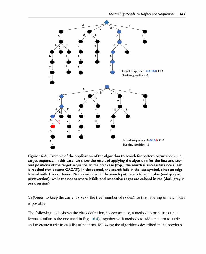
Matching Reads to Reference Sequences 341

Figure 16.3: Example of the application of the algorithm to search for pattern occurrences in atarget sequence. In this case, we show the result of applying the algorithm for the first and sec-ond positions of the target sequence. In the first case (top), the search is successful since a leafis reached (for pattern GAGAT). In the second, the search fails in the last symbol, since an edgelabeled with T is not found. Nodes included in the search path are colored in blue (mid gray inprint version), while the nodes where it fails and respective edges are colored in red (dark gray inprint version).

(self.num) to keep the current size of the tree (number of nodes), so that labeling of new nodes

is possible.

The following code shows the class definition, its constructor, a method to print tries (in a

format similar to the one used in Fig. 16.4), together with methods to add a pattern to a trie

and to create a trie from a list of patterns, following the algorithms described in the previous

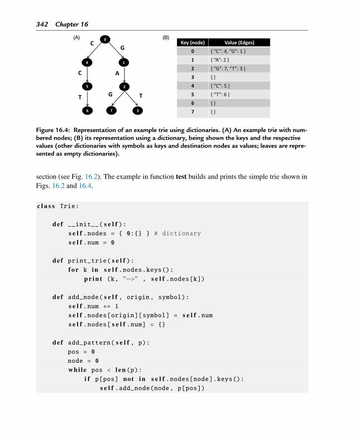
342 Chapter 16

Figure 16.4: Representation of an example trie using dictionaries. (A) An example trie with num-bered nodes; (B) its representation using a dictionary, being shown the keys and the respectivevalues (other dictionaries with symbols as keys and destination nodes as values; leaves are repre-sented as empty dictionaries).

section (see Fig. 16.2). The example in function test builds and prints the simple trie shown inFigs. 16.2 and 16.4.

c l a s s Trie:

def __init__( s e l f ):s e l f .nodes = { 0:{} } # dictionarys e l f .num = 0

def print_trie( s e l f ):f o r k in s e l f .nodes.keys():

p r i n t (k, "−>" , s e l f .nodes[k])

def add_node( s e l f , origin, symbol):s e l f .num += 1s e l f .nodes[origin][symbol] = s e l f .nums e l f .nodes[ s e l f .num] = {}

def add_pattern( s e l f , p):pos = 0

node = 0

whi le pos < l e n (p):i f p[pos] not in s e l f .nodes[node].keys():

s e l f .add_node(node, p[pos])

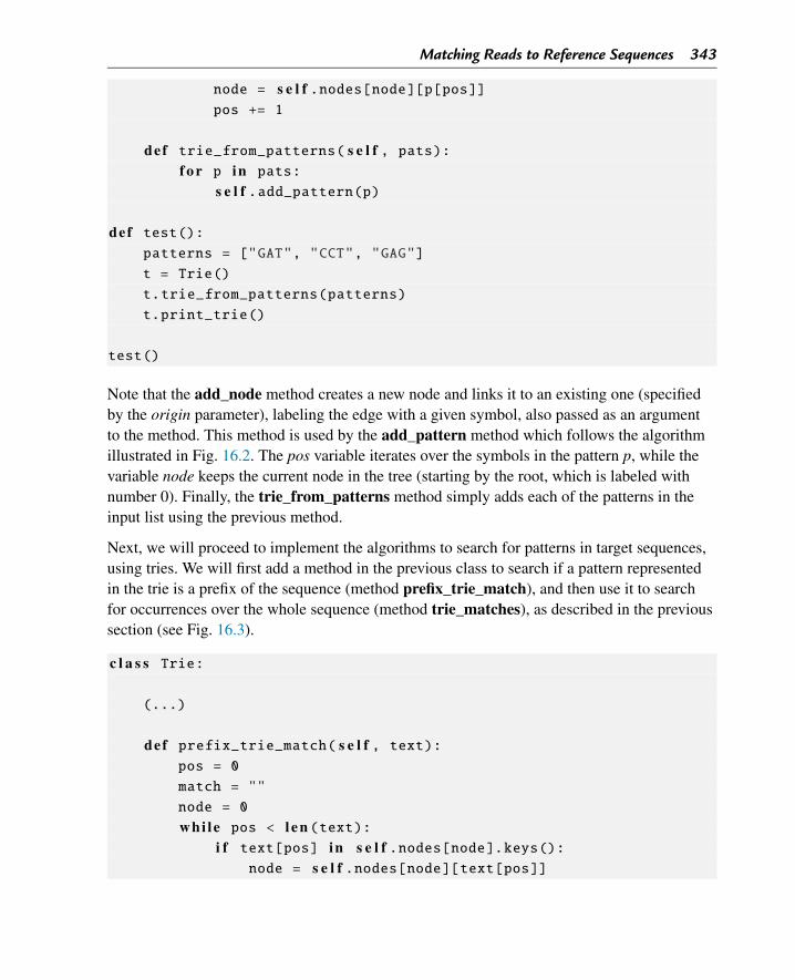
Matching Reads to Reference Sequences 343

node = s e l f .nodes[node][p[pos]]pos += 1

def trie_from_patterns( s e l f , pats):f o r p in pats:

s e l f .add_pattern(p)

def test():patterns = ["GAT", "CCT", "GAG"]

t = Trie()

t.trie_from_patterns(patterns)

t.print_trie()

test()

Note that the add_node method creates a new node and links it to an existing one (specifiedby the origin parameter), labeling the edge with a given symbol, also passed as an argumentto the method. This method is used by the add_pattern method which follows the algorithmillustrated in Fig. 16.2. The pos variable iterates over the symbols in the pattern p, while thevariable node keeps the current node in the tree (starting by the root, which is labeled withnumber 0). Finally, the trie_from_patterns method simply adds each of the patterns in theinput list using the previous method.

Next, we will proceed to implement the algorithms to search for patterns in target sequences,using tries. We will first add a method in the previous class to search if a pattern representedin the trie is a prefix of the sequence (method prefix_trie_match), and then use it to searchfor occurrences over the whole sequence (method trie_matches), as described in the previoussection (see Fig. 16.3).

c l a s s Trie:

(...)

def prefix_trie_match( s e l f , text):pos = 0

match = ""

node = 0

whi le pos < l e n (text):i f text[pos] in s e l f .nodes[node].keys():

node = s e l f .nodes[node][text[pos]]

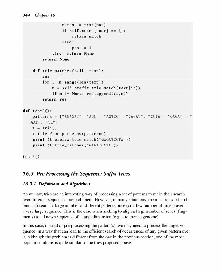
344 Chapter 16

match += text[pos]

i f s e l f .nodes[node] == {}:re turn match

e l s e :pos += 1

e l s e : re turn Nonereturn None

def trie_matches( s e l f , text):res = []

f o r i in range( l e n (text)):m = s e l f .prefix_trie_match(text[i:])i f m != None: res.append((i,m))

re turn res

def test2():patterns = ["AGAGAT", "AGC", "AGTCC", "CAGAT", "CCTA", "GAGAT", "

GAT", "TC"]

t = Trie()

t.trie_from_patterns(patterns)

p r i n t (t.prefix_trie_match("GAGATCCTA"))p r i n t (t.trie_matches("GAGATCCTA"))

test2()

16.3 Pre-Processing the Sequence: Suffix Trees

16.3.1 Definitions and Algorithms

As we saw, tries are an interesting way of processing a set of patterns to make their searchover different sequences more efficient. However, in many situations, the most relevant prob-lem is to search a large number of different patterns once (or a few number of times) overa very large sequence. This is the case when seeking to align a large number of reads (frag-ments) to a known sequence of a large dimension (e.g. a reference genome).

In this case, instead of pre-processing the pattern(s), we may need to process the target se-quence, in a way that can lead to the efficient search of occurrences of any given pattern overit. Although the problem is different from the one in the previous section, one of the mostpopular solutions is quite similar to the tries proposed above.

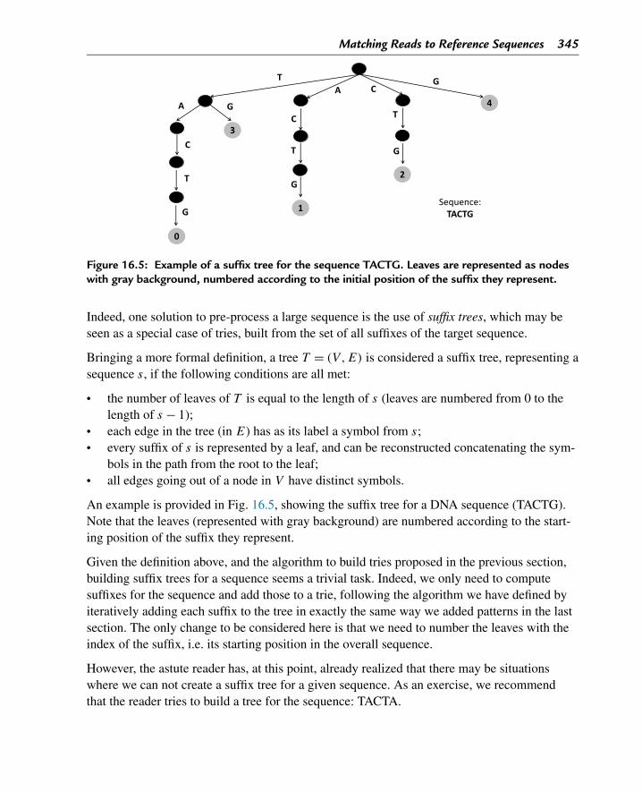
Matching Reads to Reference Sequences 345

Figure 16.5: Example of a suffix tree for the sequence TACTG. Leaves are represented as nodeswith gray background, numbered according to the initial position of the suffix they represent.

Indeed, one solution to pre-process a large sequence is the use of suffix trees, which may beseen as a special case of tries, built from the set of all suffixes of the target sequence.

Bringing a more formal definition, a tree T = (V ,E) is considered a suffix tree, representing asequence s, if the following conditions are all met:

• the number of leaves of T is equal to the length of s (leaves are numbered from 0 to thelength of s − 1);

• each edge in the tree (in E) has as its label a symbol from s;• every suffix of s is represented by a leaf, and can be reconstructed concatenating the sym-

bols in the path from the root to the leaf;• all edges going out of a node in V have distinct symbols.

An example is provided in Fig. 16.5, showing the suffix tree for a DNA sequence (TACTG).Note that the leaves (represented with gray background) are numbered according to the start-ing position of the suffix they represent.

Given the definition above, and the algorithm to build tries proposed in the previous section,building suffix trees for a sequence seems a trivial task. Indeed, we only need to computesuffixes for the sequence and add those to a trie, following the algorithm we have defined byiteratively adding each suffix to the tree in exactly the same way we added patterns in the lastsection. The only change to be considered here is that we need to number the leaves with theindex of the suffix, i.e. its starting position in the overall sequence.

However, the astute reader has, at this point, already realized that there may be situationswhere we can not create a suffix tree for a given sequence. As an exercise, we recommendthat the reader tries to build a tree for the sequence: TACTA.

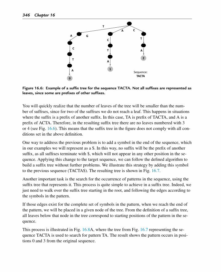
346 Chapter 16

Figure 16.6: Example of a suffix tree for the sequence TACTA. Not all suffixes are represented asleaves, since some are prefixes of other suffixes.

You will quickly realize that the number of leaves of the tree will be smaller than the num-ber of suffixes, since for two of the suffixes we do not reach a leaf. This happens in situationswhere the suffix is a prefix of another suffix. In this case, TA is prefix of TACTA, and A is aprefix of ACTA. Therefore, in the resulting suffix tree there are no leaves numbered with 3or 4 (see Fig. 16.6). This means that the suffix tree in the figure does not comply with all con-ditions set in the above definition.

One way to address the previous problem is to add a symbol in the end of the sequence, whichin our examples we will represent as a $. In this way, no suffix will be the prefix of anothersuffix, as all suffixes terminate with $, which will not appear in any other position in the se-quence. Applying this change to the target sequence, we can follow the defined algorithm tobuild a suffix tree without further problems. We illustrate this strategy by adding this symbolto the previous sequence (TACTA$). The resulting tree is shown in Fig. 16.7.

Another important task is the search for the occurrence of patterns in the sequence, using thesuffix tree that represents it. This process is quite simple to achieve in a suffix tree. Indeed, wejust need to walk over the suffix tree starting in the root, and following the edges according tothe symbols in the pattern.

If those edges exist for the complete set of symbols in the pattern, when we reach the end ofthe pattern, we will be placed in a given node of the tree. From the definition of a suffix tree,all leaves below that node in the tree correspond to starting positions of the pattern in the se-quence.

This process is illustrated in Fig. 16.8A, where the tree from Fig. 16.7 representing the se-quence TACTA is used to search for pattern TA. The result shows the pattern occurs in posi-tions 0 and 3 from the original sequence.

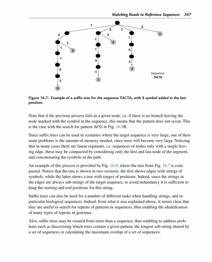
Matching Reads to Reference Sequences 347

Figure 16.7: Example of a suffix tree for the sequence TACTA, with $ symbol added in the lastposition.

Note that if the previous process fails in a given node, i.e. if there is no branch leaving thenode marked with the symbol in the sequence, this means that the pattern does not occur. Thisis the case with the search for pattern ACG in Fig. 16.8B.

Since suffix trees can be used in scenarios where the target sequence is very large, one of theirmain problems is the amount of memory needed, since trees will become very large. Noticingthat in many cases there are linear segments, i.e. sequences of nodes only with a single leav-ing edge, these may be compacted by considering only the first and last node of the segment,and concatenating the symbols in the path.

An example of this process is provided by Fig. 16.9, where the tree from Fig. 16.7 is com-pacted. Notice that the tree is shown in two versions: the first shows edges with strings ofsymbols, while the latter shows a tree with ranges of positions. Indeed, since the strings inthe edges are always sub-strings of the target sequence, to avoid redundancy it is sufficient tokeep the starting and end positions for this string.

Suffix trees can also be used for a number of different tasks when handling strings, and inparticular biological sequences. Indeed, from what it was explained above, it seems clear thatthey are useful to search for repeats of patterns in sequences, thus enabling the identificationof many types of repeats in genomes.

Also, suffix trees may be created from more than a sequence, thus enabling to address prob-lems such as discovering which trees contain a given pattern, the longest sub-string shared bya set of sequences or calculating the maximum overlap of a set of sequences.

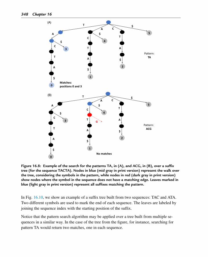
348 Chapter 16

Figure 16.8: Example of the search for the patterns TA, in (A), and ACG, in (B), over a suffixtree (for the sequence TACTA). Nodes in blue (mid gray in print version) represent the walk overthe tree, considering the symbols in the pattern, while nodes in red (dark gray in print version)show nodes where the symbol in the sequence does not have a matching edge. Leaves marked inblue (light gray in print version) represent all suffixes matching the pattern.

In Fig. 16.10, we show an example of a suffix tree built from two sequences: TAC and ATA.Two different symbols are used to mark the end of each sequence. The leaves are labeled byjoining the sequence index with the starting position of the suffix.

Notice that the pattern search algorithm may be applied over a tree built from multiple se-quences in a similar way. In the case of the tree from the figure, for instance, searching forpattern TA would return two matches, one in each sequence.

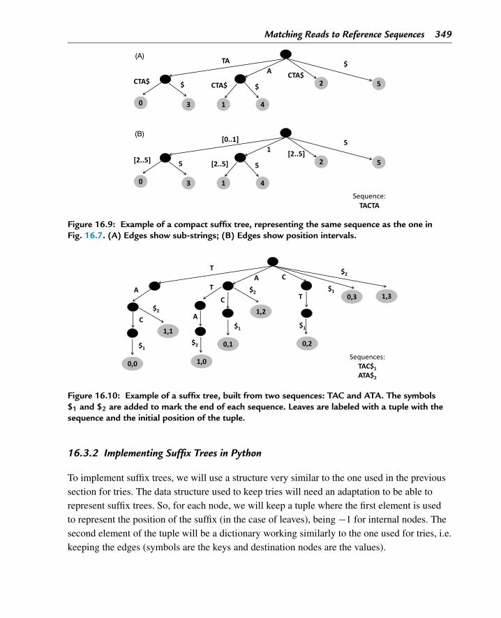
Matching Reads to Reference Sequences 349

Figure 16.9: Example of a compact suffix tree, representing the same sequence as the one inFig. 16.7. (A) Edges show sub-strings; (B) Edges show position intervals.

Figure 16.10: Example of a suffix tree, built from two sequences: TAC and ATA. The symbols$1 and $2 are added to mark the end of each sequence. Leaves are labeled with a tuple with thesequence and the initial position of the tuple.

16.3.2 Implementing Suffix Trees in Python

To implement suffix trees, we will use a structure very similar to the one used in the previoussection for tries. The data structure used to keep tries will need an adaptation to be able torepresent suffix trees. So, for each node, we will keep a tuple where the first element is usedto represent the position of the suffix (in the case of leaves), being −1 for internal nodes. Thesecond element of the tuple will be a dictionary working similarly to the one used for tries, i.e.keeping the edges (symbols are the keys and destination nodes are the values).

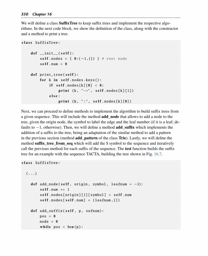
350 Chapter 16

We will define a class SuffixTree to keep suffix trees and implement the respective algo-rithms. In the next code block, we show the definition of the class, along with the constructorand a method to print a tree.

c l a s s SuffixTree:

def __init__( s e l f ):s e l f .nodes = { 0:(−1,{}) } # root nodes e l f .num = 0

def print_tree( s e l f ):f o r k in s e l f .nodes.keys():

i f s e l f .nodes[k][0] < 0:p r i n t (k, "−>", s e l f .nodes[k][1])

e l s e :p r i n t (k, ":", s e l f .nodes[k][0])

Next, we can proceed to define methods to implement the algorithm to build suffix trees froma given sequence. This will include the method add_node that allows to add a node to thetree, given the origin node, the symbol to label the edge and the leaf number (if it is a leaf; de-faults to −1, otherwise). Then, we will define a method add_suffix which implements theaddition of a suffix to the tree, being an adaptation of the similar method to add a patternin the previous section (method add_pattern of the class Trie). Lastly, we will define themethod suffix_tree_from_seq which will add the $ symbol to the sequence and iterativelycall the previous method for each suffix of the sequence. The test function builds the suffixtree for an example with the sequence TACTA, building the tree shown in Fig. 16.7.

c l a s s SuffixTree:

(...)

def add_node( s e l f , origin, symbol, leafnum = −1):s e l f .num += 1s e l f .nodes[origin][1][symbol] = s e l f .nums e l f .nodes[ s e l f .num] = (leafnum ,{})

def add_suffix( s e l f , p, sufnum):pos = 0

node = 0

whi le pos < l e n (p):

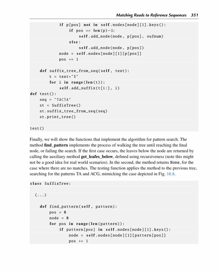
Matching Reads to Reference Sequences 351

i f p[pos] not in s e l f .nodes[node][1].keys():i f pos == l e n (p)−1:

s e l f .add_node(node, p[pos], sufnum)e l s e :

s e l f .add_node(node, p[pos])node = s e l f .nodes[node][1][p[pos]]pos += 1

def suffix_tree_from_seq( s e l f , text):t = text+"$"

f o r i in range( l e n (t)):s e l f .add_suffix(t[i:], i)

def test():seq = "TACTA"

st = SuffixTree()

st.suffix_tree_from_seq(seq)

st.print_tree()

test()

Finally, we will show the functions that implement the algorithm for pattern search. Themethod find_pattern implements the process of walking the tree until reaching the finalnode, or failing the search. If the first case occurs, the leaves below the node are returned bycalling the auxiliary method get_leafes_below, defined using recursiveness (note this mightnot be a good idea for real world scenarios). In the second, the method returns None, for thecase where there are no matches. The testing function applies the method to the previous tree,searching for the patterns TA and ACG, mimicking the case depicted in Fig. 16.8.

c l a s s SuffixTree:

(...)

def find_pattern( s e l f , pattern):pos = 0

node = 0

f o r pos in range( l e n (pattern)):i f pattern[pos] in s e l f .nodes[node][1].keys():

node = s e l f .nodes[node][1][pattern[pos]]pos += 1

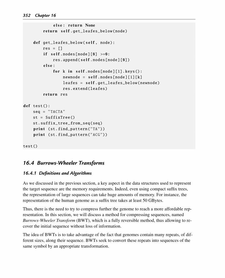
352 Chapter 16

e l s e : re turn Nonereturn s e l f .get_leafes_below(node)

def get_leafes_below( s e l f , node):res = []

i f s e l f .nodes[node][0] >=0:res.append( s e l f .nodes[node][0])

e l s e :f o r k in s e l f .nodes[node][1].keys():

newnode = s e l f .nodes[node][1][k]leafes = s e l f .get_leafes_below(newnode)res.extend(leafes)

re turn res

def test():seq = "TACTA"

st = SuffixTree()

st.suffix_tree_from_seq(seq)

p r i n t (st.find_pattern("TA"))p r i n t (st.find_pattern("ACG"))

test()

16.4 Burrows-Wheeler Transforms

16.4.1 Definitions and Algorithms

As we discussed in the previous section, a key aspect in the data structures used to representthe target sequence are the memory requirements. Indeed, even using compact suffix trees,the representation of large sequences can take huge amounts of memory. For instance, therepresentation of the human genome as a suffix tree takes at least 50 GBytes.

Thus, there is the need to try to compress further the genome to reach a more affordable rep-resentation. In this section, we will discuss a method for compressing sequences, namedBurrows-Wheeler Transform (BWT), which is a fully reversible method, thus allowing to re-cover the initial sequence without loss of information.

The idea of BWTs is to take advantage of the fact that genomes contain many repeats, of dif-ferent sizes, along their sequence. BWTs seek to convert these repeats into sequences of thesame symbol by an appropriate transformation.

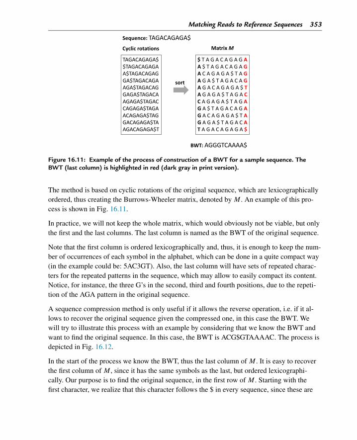
Matching Reads to Reference Sequences 353

Figure 16.11: Example of the process of construction of a BWT for a sample sequence. TheBWT (last column) is highlighted in red (dark gray in print version).

The method is based on cyclic rotations of the original sequence, which are lexicographicallyordered, thus creating the Burrows-Wheeler matrix, denoted by M . An example of this pro-cess is shown in Fig. 16.11.

In practice, we will not keep the whole matrix, which would obviously not be viable, but onlythe first and the last columns. The last column is named as the BWT of the original sequence.

Note that the first column is ordered lexicographically and, thus, it is enough to keep the num-ber of occurrences of each symbol in the alphabet, which can be done in a quite compact way(in the example could be: 5AC3GT). Also, the last column will have sets of repeated charac-ters for the repeated patterns in the sequence, which may allow to easily compact its content.Notice, for instance, the three G’s in the second, third and fourth positions, due to the repeti-tion of the AGA pattern in the original sequence.

A sequence compression method is only useful if it allows the reverse operation, i.e. if it al-lows to recover the original sequence given the compressed one, in this case the BWT. Wewill try to illustrate this process with an example by considering that we know the BWT andwant to find the original sequence. In this case, the BWT is ACG$GTAAAAC. The process isdepicted in Fig. 16.12.

In the start of the process we know the BWT, thus the last column of M . It is easy to recoverthe first column of M , since it has the same symbols as the last, but ordered lexicographi-cally. Our purpose is to find the original sequence, in the first row of M . Starting with thefirst character, we realize that this character follows the $ in every sequence, since these are

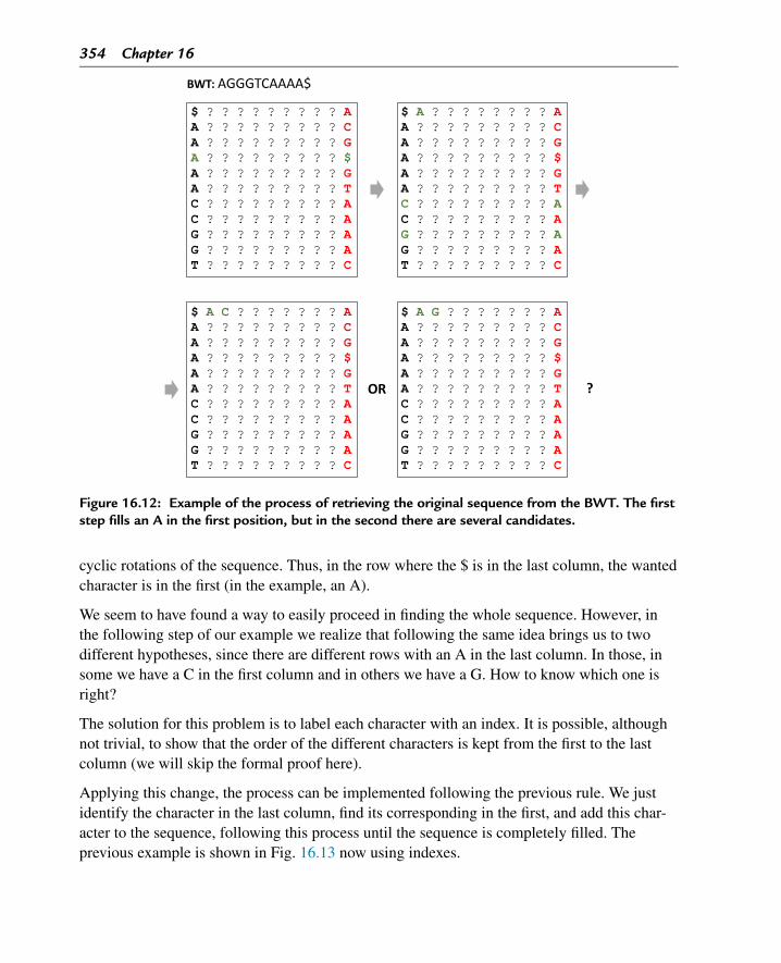
354 Chapter 16

Figure 16.12: Example of the process of retrieving the original sequence from the BWT. The firststep fills an A in the first position, but in the second there are several candidates.

cyclic rotations of the sequence. Thus, in the row where the $ is in the last column, the wantedcharacter is in the first (in the example, an A).

We seem to have found a way to easily proceed in finding the whole sequence. However, inthe following step of our example we realize that following the same idea brings us to twodifferent hypotheses, since there are different rows with an A in the last column. In those, insome we have a C in the first column and in others we have a G. How to know which one isright?

The solution for this problem is to label each character with an index. It is possible, althoughnot trivial, to show that the order of the different characters is kept from the first to the lastcolumn (we will skip the formal proof here).

Applying this change, the process can be implemented following the previous rule. We justidentify the character in the last column, find its corresponding in the first, and add this char-acter to the sequence, following this process until the sequence is completely filled. Theprevious example is shown in Fig. 16.13 now using indexes.

Matching Reads to Reference Sequences 355

Figure 16.13: Example of the process of retrieving the original sequence from the BWT, indexingthe characters. The first four steps are shown, as well as the final result.

We have seen that BWTs can provide an interesting and efficient way to compress sequences.But, along this chapter, we have been worried about pattern search. So, are BWTs good struc-tures to allow pattern search over the original sequence? The answer is positive.

To understand how to efficiently search for patterns in sequences represented as BWTs, thefirst insight is provided by the fact that, since each row in M starts with a suffix of the se-quence, all occurrences of a given pattern may be found in consecutive rows of the matrix M

356 Chapter 16

(these are order in lexicographic order). As an example, in Fig. 16.11, the three occurrences ofthe pattern AGA can be found in the fourth, fifth, and sixth rows of M .

However, we do not keep the whole matrix M and, as such, we need an algorithm that cansearch for these patterns only using the first column and the BWT (the last column). Thestrategy is based on some of the ideas used for recovering the original sequence from theBWT. We will identify the pattern in its reverse order moving within rows of the first and lastcolumns.

The first step is to identify the last symbol of the pattern and check the interval of positionswhere it matches in the last column, transposing these positions into the respective intervalover the first column (notice all equal characters are consecutive in this column). The range ofpositions is represented by two pointers: top and bottom.

Then, we will move to the next symbol (moving backwards in the pattern) and check whereit matches (in the last column), within the sub-set given by the current range. Again, thetransposition of these matches to the first column allows to update the range (top and bottompointers). This process iterates until all symbols in the pattern match, a case where the lastrange marks the rows in the matrix where there are matches. Also, the process may terminatein failing to find the pattern when the symbol in the pattern does not occur in the last columnin the defined range.

The algorithm is depicted in Fig. 16.14, where the BWT from Fig. 16.11 is used to find thepattern AGA.

Notice that the previous algorithm may be used to rapidly find if the pattern occurs and thenumber of occurrences. Still, to know the positions where the pattern occurs, extra work needsto be done. One option is to recover the first position of each row where the pattern occurs,by following the first column-last column process we saw before until reaching the $ symbol.However, in practice, this is commonly to slow to be useful, given the size of the sequence.

An alternative is to combine BWTs with a structure named as suffix arrays. Basically, a suffixarray keeps a list of the starting position of the suffix kept in each row of the matrix M . Forinstance, for the matrix in Fig. 16.11, the suffix array would be: [10,9,3,7,1,5,4,8,2,6,0].Building this structure allows to immediately be able to recover the positions of occurrenceof the pattern from the result of the previous algorithm. However, since these are structuresthat have a size equal to the original sequence, their use may be prohibitive in practice. Onealternative is to keep partial suffix arrays for a small proportion (1/K) of the positions. Thus,to find a position the last column-first column would only be needed for at most K iterations,while the memory needed would be reduced by a factor of K .

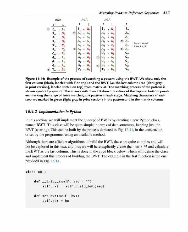
Matching Reads to Reference Sequences 357

Figure 16.14: Example of the process of searching a pattern using the BWT. We show only thefirst column (black, labeled with F on top) and the BWT, i.e. the last column (red [dark grayin print version], labeled with L on top) from matrix M . The matching process of the pattern isshown symbol by symbol. The arrows with T and B show the values of the top and bottom point-ers marking the range of rows matching the pattern in each stage. Matching characters in eachstep are marked in green (light gray in print version) in the pattern and in the matrix columns.

16.4.2 Implementation in Python

In this section, we will implement the concept of BWTs by creating a new Python class,named BWT. This class will be quite simple in terms of data structures, keeping just theBWT (a string). This can be built by the process depicted in Fig. 16.11, in the constructor,or set by the programmer using an available method.

Although there are efficient algorithms to build the BWT, these are quite complex and willnot be explored in this text, and thus we will here explicitly create the matrix M and calculatethe BWT as the last column. This is done in the code block below, which will define the classand implement this process of building the BWT. The example in the test function is the oneprovided in Fig. 16.11.

c l a s s BWT:

def __init__( s e l f , seq = ""):s e l f .bwt = s e l f .build_bwt(seq)

def set_bwt( s e l f , bw):s e l f .bwt = bw

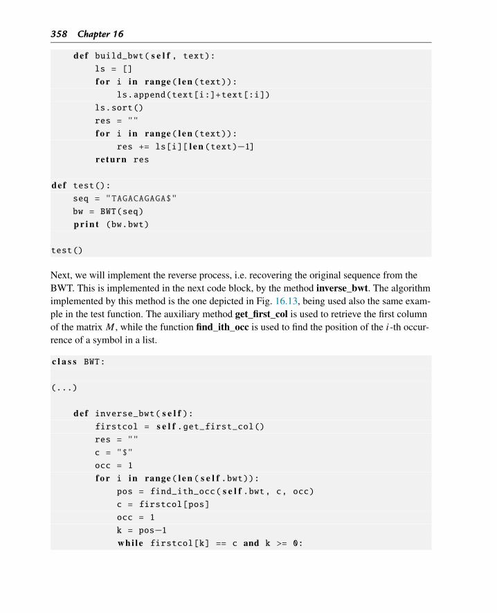
358 Chapter 16

def build_bwt( s e l f , text):ls = []

f o r i in range( l e n (text)):ls.append(text[i:]+text[:i])

ls.sort()

res = ""

f o r i in range( l e n (text)):res += ls[i][ l e n (text)−1]

re turn res

def test():seq = "TAGACAGAGA$"

bw = BWT(seq)

p r i n t (bw.bwt)

test()

Next, we will implement the reverse process, i.e. recovering the original sequence from theBWT. This is implemented in the next code block, by the method inverse_bwt. The algorithmimplemented by this method is the one depicted in Fig. 16.13, being used also the same exam-ple in the test function. The auxiliary method get_first_col is used to retrieve the first columnof the matrix M , while the function find_ith_occ is used to find the position of the i-th occur-rence of a symbol in a list.

c l a s s BWT:

(...)

def inverse_bwt( s e l f ):firstcol = s e l f .get_first_col()res = ""

c = "$"

occ = 1

f o r i in range( l e n ( s e l f .bwt)):pos = find_ith_occ( s e l f .bwt, c, occ)c = firstcol[pos]

occ = 1

k = pos−1whi le firstcol[k] == c and k >= 0:

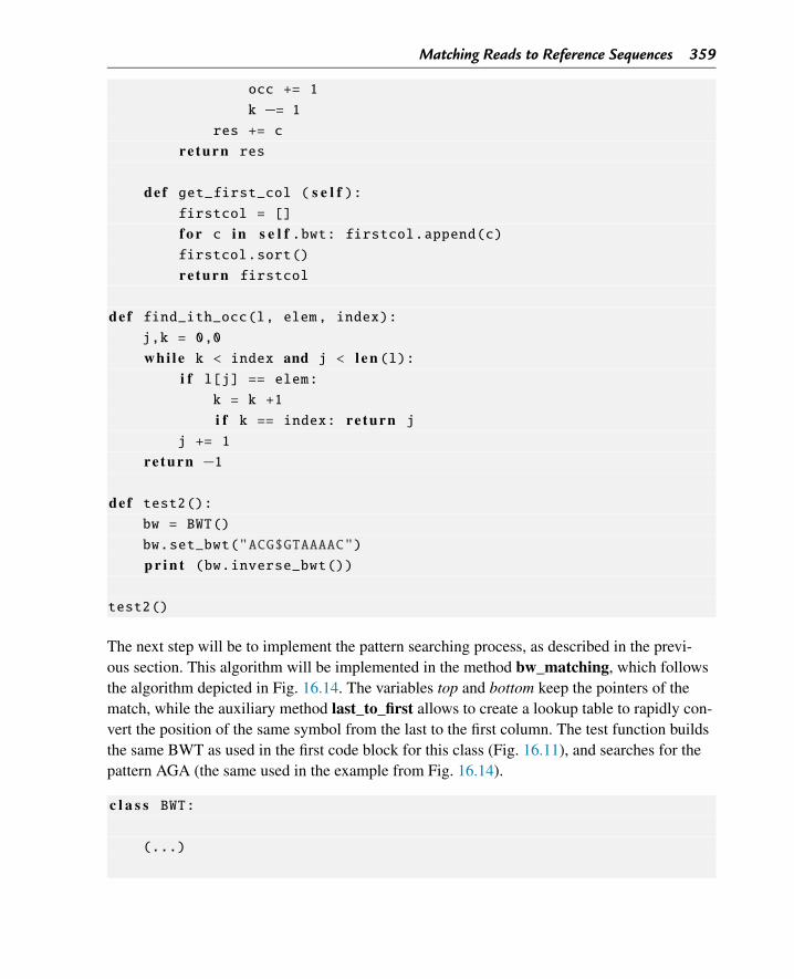
Matching Reads to Reference Sequences 359

occ += 1

k −= 1res += c

re turn res

def get_first_col ( s e l f ):firstcol = []

f o r c in s e l f .bwt: firstcol.append(c)firstcol.sort()

re turn firstcol

def find_ith_occ(l, elem, index):j,k = 0,0

whi le k < index and j < l e n (l):i f l[j] == elem:

k = k +1

i f k == index: re turn jj += 1

re turn −1

def test2():bw = BWT()

bw.set_bwt("ACG$GTAAAAC")

p r i n t (bw.inverse_bwt())

test2()

The next step will be to implement the pattern searching process, as described in the previ-ous section. This algorithm will be implemented in the method bw_matching, which followsthe algorithm depicted in Fig. 16.14. The variables top and bottom keep the pointers of thematch, while the auxiliary method last_to_first allows to create a lookup table to rapidly con-vert the position of the same symbol from the last to the first column. The test function buildsthe same BWT as used in the first code block for this class (Fig. 16.11), and searches for thepattern AGA (the same used in the example from Fig. 16.14).

c l a s s BWT:

(...)

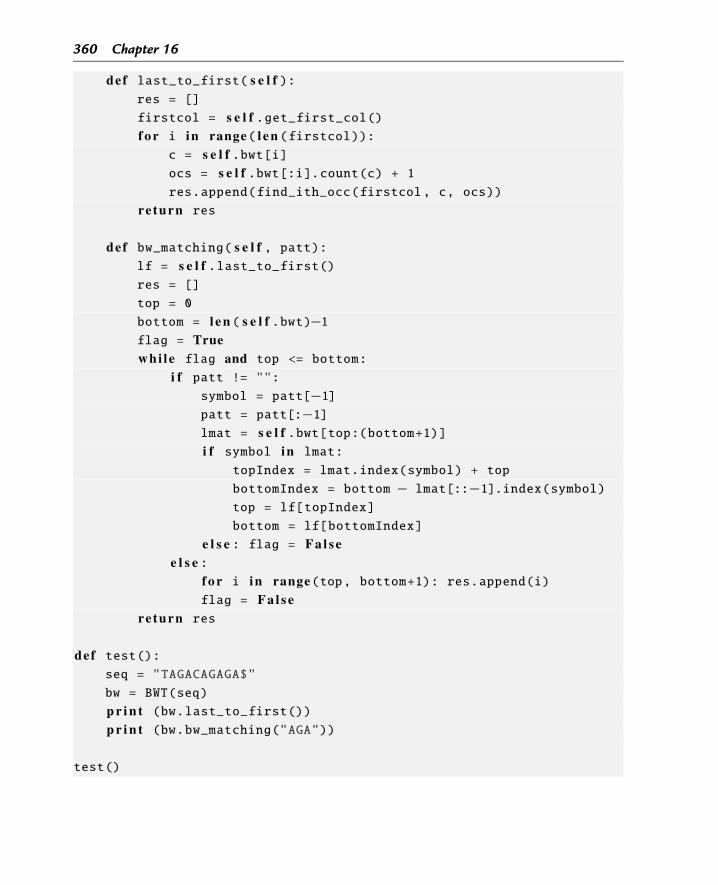
360 Chapter 16

def last_to_first( s e l f ):res = []

firstcol = s e l f .get_first_col()f o r i in range( l e n (firstcol)):

c = s e l f .bwt[i]ocs = s e l f .bwt[:i].count(c) + 1res.append(find_ith_occ(firstcol, c, ocs))

re turn res

def bw_matching( s e l f , patt):lf = s e l f .last_to_first()res = []

top = 0

bottom = l e n ( s e l f .bwt)−1flag = Truewhi l e flag and top <= bottom:

i f patt != "":symbol = patt[−1]patt = patt[:−1]lmat = s e l f .bwt[top:(bottom+1)]i f symbol in lmat:

topIndex = lmat.index(symbol) + top

bottomIndex = bottom − lmat[::−1].index(symbol)top = lf[topIndex]

bottom = lf[bottomIndex]

e l s e : flag = F a l s ee l s e :

f o r i in range(top, bottom+1): res.append(i)flag = F a l s e

re turn res

def test():seq = "TAGACAGAGA$"

bw = BWT(seq)

p r i n t (bw.last_to_first())p r i n t (bw.bw_matching("AGA"))

test()

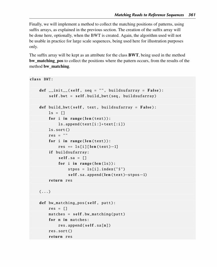
Matching Reads to Reference Sequences 361

Finally, we will implement a method to collect the matching positions of patterns, usingsuffix arrays, as explained in the previous section. The creation of the suffix array willbe done here, optionally, when the BWT is created. Again, the algorithm used will notbe usable in practice for large scale sequences, being used here for illustration purposesonly.

The suffix array will be kept as an attribute for the class BWT, being used in the methodbw_matching_pos to collect the positions where the pattern occurs, from the results of themethod bw_matching.

c l a s s BWT:

def __init__( s e l f , seq = "", buildsufarray = F a l s e ):s e l f .bwt = s e l f .build_bwt(seq, buildsufarray)

def build_bwt( s e l f , text, buildsufarray = F a l s e ):ls = []

f o r i in range( l e n (text)):ls.append(text[i:]+text[:i])

ls.sort()

res = ""

f o r i in range( l e n (text)):res += ls[i][ l e n (text)−1]

i f buildsufarray:s e l f .sa = []f o r i in range( l e n (ls)):

stpos = ls[i].index("$")

s e l f .sa.append( l e n (text)−stpos−1)re turn res

(...)

def bw_matching_pos( s e l f , patt):res = []

matches = s e l f .bw_matching(patt)f o r m in matches:

res.append( s e l f .sa[m])res.sort()

re turn res

362 Chapter 16

def test():seq = "TAGACAGAGA$"

bw = BWT(seq, True)p r i n t ("Suffix array:", bw.sa)p r i n t (bw.bw_matching_pos("AGA"))

test()

16.4.3 Aligning References to Genomes in Practice

Short read mappers have been developed following sequencing technologies. These tools areoptimized to map dozens of millions of short reads (smaller than 100 nucleotides), with veryhigh similarity (> 98%) to reference sequence and with one or fewer matches. When theseassumptions are not met, the required changes in the alignment parameters usually result inslower alignment with considerably less accuracy.

BWT-based methods can efficiently handle reads with multiple matches, originating for in-stance from repeat regions of the genome, since these regions are scanned only once. How-ever, these methods have no established way to handle the variability, either due to sequencingerrors or variation, with respect to the reference sequence.

This type of approximate matching can still be achieved by BWTs with some minor changes.Without detailing here the algorithm, we can illustrate these changes by noticing thatif our sequence has size k and there is at most 1 mismatch, there is an exact match ofat least size k/2 − 1. If we look for exact matches of this size, we can then extend thematch.

Thus, we can still use a variant of the fast algorithms discussed above for this case. Allowingfor a higher number of mismatches will result in slower mapping. Examples of methods basedon BWTs, largely used by the Bioinformatics community, include BWA [100], Bowtie2 [93],SOAP [102], or GEM [107]. As the development of sequencing technologies delivers substan-tially longer reads, novel methods, or adaptations of existing ones will be required.

Bibliographic Notes and Further Reading

Tries were firstly described by De La Briandais in 1959 [45]. Suffix trees were introduced byWeiner in 1973 [154]. BWTs were proposed in 1994 by Burrows and Wheeler [32], and anefficient implementation of BWTs was proposed by [64].

Matching Reads to Reference Sequences 363

Exercises and Programming Projects

Exercises

1. Implement a method repeats(self, k, ocs), to add to the class SuffixTree that returns a listof patterns of size k, that occur in the tree (or in the sequence used to build it) a numberof times of at least ocs.

2. Consider the definition of suffix trees representing two sequences made above, and illus-trated in Fig. 16.10.a. Write a method to add to class SuffixTree that given two sequences S1 and S2 (ter-

minating with $1 and $2, respectively) builds the suffix tree representing both. Uselabels in the leaves in the form of a tuple (sequence, initial position of the suffix).

b. Adapt the method to find patterns in the suffix tree to account for trees built from theprevious method.

c. Write another method in the same class that, assuming the tree represents two se-quences, identifies the largest sub-string that is shared by both sequences.

3. a. Consider the class BWT defined in this chapter. Complete the following code so thatit prints the sequence: CTTTAAACC$:

seq = "..."

bw = BWT(seq)

p r i n t (bw.bwt)

b. Write the code in Python to be able to reach the answer to the previous question.

Programming Projects

1. Consider the definition of compact trees provided above and the example in Fig. 16.9.a. Implement a method that builds a compact suffix tree from a sequence.b. Implement a method to add to the class SuffixTree that allows to compact a tree

(self ) that is not compacted.c. Implement a method that allows to search patterns over compacted trees.

CHAPTER 17

Further Reading and Resources

In this chapter, we will provide some useful links for the interested reader to deepen theknowledge on Bioinformatics algorithms and tools. We will discuss books with comple-mentary material, educational resources (online courses and sites with relevant resources),journals and conferences in the field, as well as provide a list with a few courses (mainly mas-ters) from universities around the world.

17.1 Complementary Books

There are many published books that can be used to complement the present text in differentways, that encompass books on Bioinformatics, general-purpose algorithms and programmingconcepts, and more specific Python programming. We will try to mention a few from eachgroup, obviously not attempting to cover the full portfolio of offers, but rather selecting a fewexamples known by the authors.

Regarding Bioinformatics books, most of the available texts are written by biologists or otherbiology-related professionals, being written mostly for an audience seeking to improve theirskills on using Bioinformatics tools and understanding their results, and not so much for pro-grammers.

From this offer we would select the books by David Mount [117] and Jonathan Pevsner [125].Indeed, these are two very comprehensive books covering a large set of concepts, algorithms,and tools in Bioinformatics, combining well the definition of the methods and their main fea-tures, with the use of tools implementing these methods and the interpretation of their resultsin a critical perspective. Both these books cover most of the topics we address in this book,while not focusing on the implementation of the methods using a programming language, as itis done here. The latter is also more updated as it has a 2015 edition, while the former had itslast edition in 2004.

For a more algorithmic oriented discussion of Bioinformatics, the work of Pavel Pevzner’sgroup is one of the most important efforts. We would emphasize here the first book in col-laboration with Neil Jones [84], which covers a number of problems in Bioinformatics andaddresses the main algorithmic classes to address these tasks. More recently, in collaborationwith Phlippe Compeau, the same author has published a two volume book [35], also focused

Bioinformatics Algorithms. DOI: 10.1016/B978-0-12-812520-5.00017-1Copyright © 2018 Elsevier Inc. All rights reserved. 365

366 Chapter 17

on algorithms to address Bioinformatics problems, motivated in every chapter by a specific bi-ological problem. Although it does not provide implementations of the algorithms, it providesa comprehensive review of the most important algorithmic core topics for Bioinformatics ap-plications.

An important contribution in the same line was the book by Böckenhauer and Bongartz from2007 [28], which covers a relevant set of algorithms mainly related with sequence/string pro-cessing. This is the ideal book for readers who are comfortable with a more formal approachusing a Mathematical notation of the main algorithms.

The number of books providing complementary concepts regarding algorithms and program-ming is very vast, and of course out of the scope here. However, we can mention the book byDan Gusfield [70] and [39] related to string-based algorithms, while the books by Sedgewickand Wayne [138] and Wirth [155] provide a more general-purpose coverage of algorithms anddata structures.

Also, there are a few books with a more practical focus on applications of the Python pro-gramming language to Bioinformatics. One of these examples is the book by Sebastian Bassi,recently with its 2nd edition [25], which covers the main concepts in Python programmingproviding a number of examples for biological data and also addressing the basics of Bio-Python. The book by Mitchel Model [115] follows a similar approach focusing the explana-tion on the Python concepts. These are good books to work over Python programming skills,with a flavor of Bioinformatics. Still, they are not focused on the algorithmic aspects of themain Bioinformatics tools and tasks.

17.2 Journals and Conferences

Bioinformatics is a multidisciplinary area, and thus many of the important papers on Bioin-formatics tools are spread along journals and conferences of different topics, from computerscience to specific biological and biomedical venues. Still, there are a few important journalsmainly devoted to this field, or that have specific tracks for Bioinformatics work.

The following list provides an overview of some selected journals and their publishers, and abrief description of their contents:

• Bioinformatics (Oxford University Press) – probably the most important journal for thisarea, focuses mainly on new developments in genome bioinformatics and computationalbiology. Two sections – Discovery Notes and Application Notes – focus on shorter pa-pers reporting biologically interesting discoveries using computational methods, and thedevelopment of bioinformatics applications.

Further Reading and Resources 367

• Nucleic Acids Research (Oxford University Press) – its focus are physical, chemical,biochemical and biological aspects of nucleic acids and proteins involved in nucleicacid metabolism and/or interactions; although not a specific Bioinformatics journal, it isknown for publishing yearly comprehensive reviews of available databases and web appli-cations in all fields of Bioinformatics; even in the regular issues it publishes many articleson software applications to biological problems.

• Briefings in Bioinformatics (Oxford University Press) – it is an international forum forresearchers and educators in the life sciences, publishing reviews of databases and tools ofgenetics, molecular, and systems biology providing practical guidance in Bioinformaticsapproaches.

• PLOS Computational Biology (PLOS) – features studies that focus on the understandingand modeling of living systems in different scales, from cells to populations or ecosys-tems through the application of computational methods.

• BMC Bioinformatics (Biomed Central) – open-access journal that publishes papers on thedifferent aspects of the development, testing and application of bioinformatics methodsfor the modeling and analysis of biological data, and other areas of computational biology.

• Computer Methods and Programs in Biomedicine (Elsevier) – publishes articles related tocomputing methodology and software in all aspects of biomedical research and medicalpractice.

• Computers in Biology and Medicine (Elsevier) – publishes research results related to theapplication of computers to the fields of bioscience and medicine.

• Algorithms for Molecular Biology (Biomed Central) – publishes articles on algorithmsfor biological sequence and structure analysis, phylogeny reconstruction, and machinelearning.

Regarding international conferences, we list here a few of the most relevant for the Bioinfor-matics field:

• Inteligent Systems for Molecular Biology (ISMB), will have its 26th edition in 2018, be-ing probably the largest and most important venue for Bioinformatics related research,bringing together researchers from computer science, molecular biology, mathematics,statistics, and related fields.

• European Conference on Computational Biology (ECCB), will have its 17th edition in2018, being the main European event in Bioinformatics and Computational Biology.

• RECOMB, already having its 22nd edition in 2018, aims to bridge the areas of computa-tional, mathematical, statistical, and biological sciences.

• IEEE International Conference on Bioinformatics and Biomedicine (BIBM), is the mainIEEE sponsored conference related to Bioinformatics and health informatics.

368 Chapter 17

• ACM Conference on Bioinformatics, Computational Biology, and Health Informatics(ACM BCB), the flagship conference of the interest group in Bioinformatics for the ACM,already with 8 editions.

• Pacific Symposium in Biocomputing (PSB) – always located in Hawaii, it is a multi-disciplinary conference for the discussion of research in the theory and application ofcomputational methods in problems of biological significance, being a conference witha considerable tradition in the field.

• Workshop on Algorithms in Bioinformatics (WABI) – already with 17 editions, coversall research in algorithmic work in bioinformatics, computational biology, and systemsbiology.

• International Conference on Practical Applications of Computational Biology & Bioin-formatics (PACBB), being a forum already in its 12th edition, mainly for the discussion ofpractical approaches of Bioinformatics for junior researchers.

17.3 Formal Education

Around the world, there are nowadays many different universities offering degrees in thefields of Bioinformatics and Computational Biology. As we did in previous sections, we re-view here some examples of this offer, seeking to select degrees spread around the worldin institutions known by their quality. Since most of the available degrees are in the masterslevel, we provide here a number of MSc’s in Bioinformatics, which are available for studentswith a background on Biology (or other biological/biomedical field) or Computer Science (orrelated degrees in Informatics or Information Technologies).

• MSc Bioinformatics, Johns Hopkins Institute, USA – http://advanced.jhu.edu/academics/graduate-degree-programs/bioinformatics – available in a fully on-line version;

• MSc Bioinformatics and Systems Biology, Univ. California San Diego, USA – http://bioinformatics.ucsd.edu/curriculum – strong component of modeling and Sys-tems Biology, very research oriented;

• Master Computational Biology and Bioinformatics, ETH Zurich, Switzerland – http://www.cbb.ethz.ch/;

• MSc Bioinformatics – Vrije Univ., Amsterdam, Netherlands – http://masters.vu.nl/en/programmes/bioinformatics-systems-biology;

• MSc Bioinformatics and Systems Biology, University of Manchester, UK – https://www.bmh.manchester.ac.uk/biology/study/masters/bioinformatics-systems

-biology/;• MSc Bioinformatics, Univ. Minho, Portugal – http://bioinformatica.di.uminho.pt;

Further Reading and Resources 369

• MSc Bioinformatics, South African National Bioinformatics Institute, South Africa –http://www.sanbi.ac.za/training-2/msc-bioinformatics/;

• Master of Computational Biology, University of Melbourne, Australia – http://science-courses.unimelb.edu.au/study/degrees/master-of-computational-

biology/;• Master Bioinformatics, Univ. Beijing, China – http://school.cucas.edu.cn/Beijing-Normal-University-27/program/Bioinformatics-4234.html;

• MSc Bioinformatics, Nanyang Technological Institute, Singapore – http://sce.ntu.edu.sg/Programmes/CurrentStudents/Graduate/Pages/msc-bioinformatics-

intro.aspx.

Apart from these integrated pedagogical offers, most universities, and other research institu-tions, offer a number of courses in specific subjects related to Bioinformatics. We select nextjust a few examples:

• University of Cambridge (UK), Bioinformatics Training – http://bioinfotraining.bio.cam.ac.uk;

• Brabaham Institute (UK), Bioinformatics Training – http://www.bioinformatics.babraham.ac.uk/training.html;

• Vienna Biocenter (Austria), BioComp training – http://biocomp.vbcf.ac.at/training;

• Dutch TechCenter for the Life Sciences (Netherlands) – https://www.dtls.nl/courses;

• Gulbenkian Training Programme in Bioinformatics (Portugal) – http://gtpb.igc.gulbenkian.pt/bicourses;

• ECSeq Bioinformatics (Germany; company) – http://ecseq.com/;• Cold Spring Harbor Lab. (USA) – http://meetings.cshl.edu/courseshome.aspx;• UC Davis Bioinformatics core (USA) – http://bioinformatics.ucdavis.edu/training;

• Bioinformatics.ca workshops (Canada) – https://bioinformatics.ca/workshops-2017.

These and other resources can be searched using portals as the one of the Global Organisa-tion for Bioinformatics Learning, Education & Training (GOBLET), available in http://mygoblet.org/training-portal.

17.4 Online Resources

In the last few years, we have been observing a large growth in the number of available onlinecourses, spread by multiple platforms. The presence of courses related to Bioinformatics and

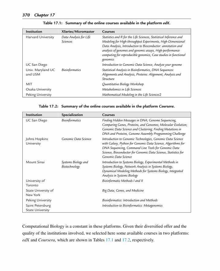
370 Chapter 17

Table 17.1: Summary of the online courses available in the platform edX.

Institution XSeries/Micromaster Courses

Harvard University Data Analysis for LifeSciences

Statistics and R for the Life Sciences, Statistical Inference andModeling for High-throughput Experiments, High-DimensionalData Analysis, Introduction to Bioconductor: annotation andanalysis of genomes and genomic assays, High-performancecomputing for reproducible genomics, Case studies in functionalgenomics

UC San Diego Introduction to Genomic Data Science, Analyze your genome

Univ. Maryland UCand USM

Bioinformatics Statistical Analysis in Bioinformatics, DNA Sequences:Alignments and Analysis, Proteins: Alignment, Analysis andStructure

MIT Quantitative Biology Workshop

Osaka University Metabolomics in Life Sciences

Peking University Mathematical Modeling in the Life Sciences2

Table 17.2: Summary of the online courses available in the platform Coursera.

Institution Specialization Courses

UC San Diego Bioinformatics Finding Hidden Messages in DNA; Genome Sequencing,Comparing Genes, Proteins, and Genomes; Molecular Evolution;Genomic Data Science and Clustering; Finding Mutations inDNA and Proteins, Genome Assembly Programming Challenge

Johns HopkinsUniversity

Genomic Data Science Introduction to Genomic Technologies, Genomic Data Sciencewith Galaxy, Python for Genomic Data Science, Algorithms forDNA Sequencing, Command Line Tools for Genomic DataScience, Bioconductor for Genomic Data Science, Statistics forGenomic Data Science

Mount Sinai Systems Biology andBiotechnology

Introduction to Systems Biology, Experimental Methods inSystems Biology, Network Analysis in Systems Biology,Dynamical Modeling Methods for Systems Biology, IntegratedAnalysis in Systems Biology

University ofToronto

Bioinformatic Methods I and II

State University ofNew York

Big Data, Genes, and Medicine

Peking University Bioinformatics: Introduction and Methods

Saint PetersburgState University

Introduction to Bioinformatics: Metagenomics

Computational Biology is a constant in these platforms. Given their diversified offer and the

quality of the institutions involved, we selected here some available courses in two platforms:

edX and Coursera, which are shown in Tables 17.1 and 17.2, respectively.

Further Reading and Resources 371

Also, there are many sites available that can be excellent resources to learn Bioinformaticsand Python programming for the life sciences. In the next list, we selected a few of those thatbe used by the reader to complement the materials of this book.

• NCBI mini-courses – https://www.ncbi.nlm.nih.gov/Class/minicourses/;• EBI Train Online – https://www.ebi.ac.uk/training/online/;• Biostars – https://www.biostars.org/, forum of frequently asked questions in Bioin-

formatics;• SeqAnswers – http://seqanswers.com/, forum of frequently asked questions when

handling next-generation sequencing data;• Rosalind – http://rosalind.info/problems/locations/, a site that allows to learn

Bioinformatics by solving programming problems;• Python for Biologists – https://pythonforbiologists.com/, resources for learning

to program in Python for people with a background in biology;• IAP (Introduction to Applied Bioinformatics) – http://readiab.org/, open source

interactive text that introduces readers to core concepts of Bioinformatics.

Final Words

We have reached the end of our journey through the sea of Bioinformatics algorithms, andwe hope it was a pleasant one. Of course, many relevant topics remained untouched, manyalgorithms are still there to be learned. Our expectation is that we have awakened in our read-ers the will to learn more about Bioinformatics, and that the resources put together in the lastchapter, and in the end of each chapter, are good starting points to proceed this journey intomore adventurous algorithms and programs.

Bioinformatics is a multidisciplinary topic and, therefore, the readers of this book probablyhave very distinct backgrounds. We hope that we were able to address this diversity and ex-plain the topics even for non-experienced readers. By understanding the ideas and algorithmsbehind the different methods we hope the readers can optimize their usage or be able to de-velop novel methods that meet their needs. The decision of having simplified algorithms andtheir Python implementation was to try to accomplish this goal. The readers will be the judgesof how this has worked in the end. We will await for their feedback.

Since the field of Bioinformatics is growing, we are expecting the number of books in thisarea to grow as well, becoming more specialized in the topics to be covered. This is a trendwe expect to see also in online and formal courses and degrees. Still, even at this point, webelieve that a general purpose overview of the main Bioinformatics algorithms is important,and we tried to fill this gap.

There were many topics we have not considered in this book, but that are important in Bioin-formatics. Maybe one of the most relevant is Machine Learning (ML), which makes the corealgorithmic support for many tasks in Bioinformatics, from gene prediction, to protein classi-fication and gene expression (or other omics) data analysis. To learn the basic algorithms andMathematical concepts underlying ML models is, indeed, very relevant for today’s Bioinfor-matics.

One of the main tasks in Bioinformatics is related to protein structure prediction, i.e. the abil-ity to design algorithms able to predict the three-dimensional configuration of the proteinbased on its sequence of aminoacids. This is also a subject we have not addressed here, which

373

Final Words

may be approached using ML or other statistical methods, based on features calculated fromthe sequences.

Genomics for personalized medicine is a research area that already has a large demand of ex-perts. Handling the vast amounts of data that are being generated by all sorts of projects, bothin research or clinical laboratories, requires well prepared and trained Bioinformatics special-ists. Tasks such as variant calling or gene differential expression were not covered in this booksince, beyond the algorithmic details, a solid statistical background is required for a good un-derstanding of these methods. Nevertheless, in this book, we have approached algorithms andmethods that form part of the steps of the data analysis pipeline.

In many topics, we also left out some important optimization algorithms, which are used toaddress complex optimization tasks in Bioinformatics. For instance, we have not covered im-portant meta-heuristics as Evolutionary Algorithms or Simulated Annealing.

In all previous cases, the decision to leave these topics out of this book was related to thecomplexity of the algorithms and underlying Mathematical and statistical concepts, given ourchoice to try to explain the main details and implement our algorithms in Python. We hope wecan cover these subjects in a future project.

We really hope you have enjoyed this book!

Miguel Rocha

Pedro G. Ferreira

374

Bibliography

[1] Gwas central, http://www.gwascentral.org/.[2] Python for beginners, http://www.python.org/doc/Intros.html.[3] The python language website, http://www.python.org/.[4] Python tutor, visualization of code execution, http://pythontutor.com/.[5] The python tutorial, https://docs.python.org/3/tutorial/.[6] Computational Methods in Molecular Biology, Elsevier Science, 1998.[7] Biopython: freely available python tools for computational molecular biology and bioinformatics,

Bioinformatics 25 (11) (2009) 1422–1423.[8] Biopython tutorial and cookbook, http://biopython.org/DIST/docs/tutorial/Tutorial.html. (Last update

Nov 23, 2016).[9] Alfred V. Aho, John E. Hopcroft, The Design and Analysis of Computer Algorithms, 1st edition,

Addison-Wesley Longman Publishing Co., Inc., Boston, MA, USA, 1974.[10] B. Alberts, A. Johnson, J. Lewis, M. Raff, K. Roberts, P. Walter, Molecular Biology of the Cell, 4th edition,

Garland Science, New York, USA, 2002.[11] Stephen F. Altschul, Warren Gish, Webb Miller, Eugene W. Myers, David J. Lipman, Basic local alignment

search tool, Journal of Molecular Biology 215 (3) (1990) 403–410.[12] Stephen F. Altschul, Thomas L. Madden, Alejandro A. Schäffer, Jinghui Zhang, Zheng Zhang, Webb Miller,

David J. Lipman, Gapped blast and psi-blast: a new generation of protein database search programs, NucleicAcids Research 25 (17) (1997) 3389–3402.

[13] R. Andersson, et al., An atlas of active enhancers across human cell types and tissues, Nature 507 (7493)(Mar 2014) 455–461.

[14] K. Asai, S. Hayamizu, K. Handa, Prediction of protein secondary structure by the hidden Markov model,Computer Applications in the Biosciences 9 (2) (Apr 1993) 141–146.

[15] A. Auton, et al., A global reference for human genetic variation, Nature 526 (7571) (Oct 2015) 68–74.[16] Gary D. Bader, Christopher W.V. Hogue, Analyzing yeast protein-protein interaction data obtained from

different sources, Nature Biotechnology 20 (10) (2002) 991–997.[17] T.L. Bailey, Discovering sequence motifs, Methods in Molecular Biology 452 (2008) 231–251.[18] T.L. Bailey, C. Elkan, Fitting a mixture model by expectation maximization to discover motifs in

biopolymers, Proceedings. International Conference on Intelligent Systems for Molecular Biology 2 (1994)28–36.

[19] Pierre Baldi, Søren Brunak, Bioinformatics: The Machine Learning Approach, 2nd edition, MIT Press,Cambridge, MA, USA, 2001.

[20] Anton Bankevich, Sergey Nurk, Dmitry Antipov, Alexey A. Gurevich, Mikhail Dvorkin, Alexander S.Kulikov, Valery M. Lesin, Sergey I. Nikolenko, Son Pham, Andrey D. Prjibelski, et al., Spades: a newgenome assembly algorithm and its applications to single-cell sequencing, Journal of Computational Biology19 (5) (2012) 455–477.

[21] Albert-László Barabási, Réka Albert, Emergence of scaling in random networks, Science 286 (5439) (1999)509–512.

375

Bibliography

[22] Albert-László Barabási, Natali Gulbahce, Joseph Loscalzo, Network medicine: a network-based approach tohuman disease, Nature Reviews Genetics 12 (1) (2011) 56–68.

[23] Albert-Laszlo Barabási, Zoltan N. Oltvai, Network biology: understanding the cell’s functional organization,Nature Reviews Genetics 5 (2) (2004) 101–113.

[24] N.L. Barbosa-Morais, M. Irimia, Q. Pan, H.Y. Xiong, S. Gueroussov, L.J. Lee, V. Slobodeniuc, C. Kutter,S. Watt, R. Colak, T. Kim, C.M. Misquitta-Ali, M.D. Wilson, P.M. Kim, D.T. Odom, B.J. Frey, B.J.Blencowe, The evolutionary landscape of alternative splicing in vertebrate species, Science 338 (6114) (Dec2012) 1587–1593.

[25] Sebastian Bassi, Python for Bioinformatics, CRC Press, 2016.[26] T. Beck, R.K. Hastings, S. Gollapudi, R.C. Free, A.J. Brookes, GWAS Central: a comprehensive resource for

the comparison and interrogation of genome-wide association studies, European Journal of Human Genetics22 (7) (Jul 2014) 949–952.

[27] E. Birney, et al., Identification and analysis of functional elements in 1% of the human genome by theENCODE pilot project, Nature 447 (7146) (Jun 2007) 799–816.

[28] Hans-Joachim Böckenhauer, Dirk Bongartz, Algorithmic Aspects of Bioinformatics, Springer-Verlag NewYork, Inc., Secaucus, NJ, USA, 2007.

[29] Robert S. Boyer, J. Strother Moore, A fast string searching algorithm, Communications of the ACM 20 (10)(October 1977) 762–772.

[30] J. Buhler, M. Tompa, Finding motifs using random projections, Journal of Computational Biology 9 (2)(2002) 225–242.

[31] C. Burge, S. Karlin, Prediction of complete gene structures in human genomic DNA, Journal of MolecularBiology 268 (1) (Apr 1997) 78–94.

[32] Michael Burrows, David J. Wheeler, A Block-Sorting Lossless Data Compression Algorithm, 1994.[33] P. Carninci, et al., The transcriptional landscape of the mammalian genome, Science 309 (5740) (Sep 2005)

1559–1563.[34] Humberto Carrillo, David Lipman, The multiple sequence alignment problem in biology, SIAM Journal on

Applied Mathematics 48 (5) (1988) 1073–1082.[35] Phillip Compeau, Pavel Pevzner, Bioinformatics Algorithms: An Active Learning Approach, Active

Learning Publishers, 2015.[36] Community Content Contributions, Boundless biology, https://www.boundless.com/biology/textbooks/

boundless-biology-textbook/, February 2017.[37] G.M. Cooper, The Cell: A Molecular Approach, 2nd edition, Sinauer Associates, Sunderland, MA, USA,

2000.[38] Thomas H. Cormen, Clifford Stein, Ronald L. Rivest, Charles E. Leiserson, Introduction to Algorithms, 2nd

edition, McGraw-Hill Higher Education, 2001.[39] Maxime Crochemore, Christophe Hancart, Thierry Lecroq, Algorithms on Strings, Cambridge University

Press, 2007.[40] G.E. Crooks, G. Hon, J.M. Chandonia, S.E. Brenner, WebLogo: a sequence logo generator, Genome

Research 14 (6) (Jun 2004) 1188–1190.[41] M.K. Das, H.K. Dai, A survey of DNA motif finding algorithms, BMC Bioinformatics 8 (Suppl 7) (Nov

2007) S21.[42] Sanjoy Dasgupta, Christos H. Papadimitriou, Umesh Vazirani, Algorithms, McGraw-Hill, Inc., 2006.[43] Margaret O. Dayhoff, Atlas of Protein Sequence and Structure, 1965.[44] N. de Bruijn, A combinatorial problem, Proceedings of the Section of Sciences of the Koninklijke

Nederlandse Akademie van Wetenschappen te Amsterdam 49 (7) (1946) 758–764.[45] Rene De La Briandais, File searching using variable length keys, in: Papers Presented at the March 3–5,

1959, Western Joint Computer Conference, ACM, 1959, pp. 295–298.

376

Bibliography

[46] T. Derrien, R. Johnson, G. Bussotti, A. Tanzer, S. Djebali, H. Tilgner, G. Guernec, D. Martin, A. Merkel,D.G. Knowles, J. Lagarde, L. Veeravalli, X. Ruan, Y. Ruan, T. Lassmann, P. Carninci, J.B. Brown,L. Lipovich, J.M. Gonzalez, M. Thomas, C.A. Davis, R. Shiekhattar, T.R. Gingeras, T.J. Hubbard,C. Notredame, J. Harrow, R. Guigo, The GENCODE v7 catalog of human long noncoding RNAs: analysisof their gene structure, evolution, and expression, Genome Research 22 (9) (Sep 2012) 1775–1789.

[47] P. D’haeseleer, What are DNA sequence motifs? Nature Biotechnology 24 (4) (Apr 2006) 423–425.[48] Reinhard Diestel, Graph Theory, 3rd edition, Graduate Texts in Mathematics, vol. 173, Springer, 2005.[49] I. Dunham, et al., An integrated encyclopedia of DNA elements in the human genome, Nature 489 (7414)

(Sep 2012) 57–74.[50] R. Durbin, S. Eddy, A. Krogh, G. Mitchison, Biological Sequence Analysis: Probabilistic Models of Proteins

and Nucleic Acids, Cambridge University Press, 1998.[51] J.R. Ecker, W.A. Bickmore, I. Barroso, J.K. Pritchard, Y. Gilad, E. Segal, Genomics: ENCODE explained,

Nature 489 (7414) (Sep 2012) 52–55.[52] S.R. Eddy, Multiple alignment using hidden Markov models, Proceedings. International Conference on

Intelligent Systems for Molecular Biology 3 (1995) 114–120.[53] S.R. Eddy, Hidden Markov models, Current Opinion in Structural Biology 6 (3) (Jun 1996) 361–365.[54] S.R. Eddy, What is a hidden Markov model? Nature Biotechnology 22 (10) (Oct 2004) 1315–1316.[55] S.R. Eddy, A probabilistic model of local sequence alignment that simplifies statistical significance

estimation, PLoS Computational Biology 4 (5) (May 2008) e1000069.[56] S.R. Eddy, A new generation of homology search tools based on probabilistic inference, Genome

Informatics 23 (1) (Oct 2009) 205–211.[57] S.R. Eddy, Accelerated profile HMM searches, PLoS Computational Biology 7 (10) (Oct 2011) e1002195.[58] Robert C. Edgar, Muscle: multiple sequence alignment with high accuracy and high throughput, Nucleic

Acids Research 32 (5) (2004) 1792–1797.[59] E. Eskin, P.A. Pevzner, Finding composite regulatory patterns in DNA sequences, Bioinformatics

18 (Suppl 1) (2002) S354–S363.[60] Leonhard Euler, Solutio problematis ad geometriam situs pertinentis, Commentarii Academiae Scientiarum

Petropolitanae 8 (1741) 128–140.[61] Even Shimon, Graph Algorithms, 2nd edition, Cambridge University Press, New York, NY, USA, 2011.[62] Joseph Felsenstein, Inferring Phylogenies, vol. 2, Sinauer Associates, Sunderland, MA, 2004.[63] Da-Fei Feng, Russell F. Doolittle, Progressive sequence alignment as a prerequisitetto correct phylogenetic

trees, Journal of Molecular Evolution 25 (4) (1987) 351–360.[64] Paolo Ferragina, Giovanni Manzini, Opportunistic data structures with applications, in: Foundations of

Computer Science, 2000. Proceedings. 41st Annual Symposium on, IEEE, 2000, pp. 390–398.[65] P.G. Ferreira, P.J. Azevedo, Evaluating deterministic motif significance measures in protein databases,

Algorithms for Molecular Biology 2 (Dec 2007) 16.[66] Jeffrey E.F. Friedl, Mastering Regular Expressions, 2nd edition, O’Reilly & Associates, Inc., Sebastopol,

CA, USA, 2002.[67] Emanuel Gonçalves, Joachim Bucher, Anke Ryll, Jens Niklas, Klaus Mauch, Steffen Klamt, Miguel Rocha,

Julio Saez-Rodriguez, Bridging the layers: towards integration of signal transduction, regulation andmetabolism into mathematical models, Molecular BioSystems 9 (7) (2013) 1576–1583.

[68] M. Gribskov, S. Veretnik, Identification of sequence pattern with profile analysis, Methods in Enzymology266 (1996) 198–212.

[69] Stéphane Guindon, Jean-François Dufayard, Vincent Lefort, Maria Anisimova, Wim Hordijk, OlivierGascuel, New algorithms and methods to estimate maximum-likelihood phylogenies: assessing theperformance of PhyML 3.0, Systematic Biology 59 (3) (2010) 307–321.

[70] Dan Gusfield, Algorithms on Strings, Trees and Sequences: Computer Science and Computational Biology,1st edition, Cambridge University Press, May 1997.

[71] Frank Harary, Graph Theory, Addison-Wesley, 1972.

377

Bibliography

[72] J. Harrow, A. Frankish, J.M. Gonzalez, E. Tapanari, M. Diekhans, F. Kokocinski, B.L. Aken, D. Barrell,A. Zadissa, S. Searle, I. Barnes, A. Bignell, V. Boychenko, T. Hunt, M. Kay, G. Mukherjee, J. Rajan,G. Despacio-Reyes, G. Saunders, C. Steward, R. Harte, M. Lin, C. Howald, A. Tanzer, T. Derrien, J. Chrast,N. Walters, S. Balasubramanian, B. Pei, M. Tress, J.M. Rodriguez, I. Ezkurdia, J. van Baren, M. Brent,D. Haussler, M. Kellis, A. Valencia, A. Reymond, M. Gerstein, R. Guigo, T.J. Hubbard, GENCODE: thereference human genome annotation for The ENCODE Project, Genome Research 22 (9) (Sep 2012)1760–1774.

[73] D. Haussler, A. Krogh, I.S. Mian, K. Sjolander, Protein modeling using hidden Markov models: analysis ofglobins, in: Proceeding of the Twenty-Sixth Hawaii International Conference on System Sciences, IEEE,IEEE, 1993, pp. 792–802.

[74] Steven Henikoff, Jorja G. Henikoff, Amino acid substitution matrices from protein blocks, Proceedings ofthe National Academy of Sciences 89 (22) (1992) 10915–10919.

[75] G.Z. Hertz, G.W. Hartzell, G.D. Stormo, Identification of consensus patterns in unaligned DNA sequencesknown to be functionally related, Computer Applications in the Biosciences 6 (2) (Apr 1990) 81–92.

[76] Carl Hierholzer, Über die Möglichkeit, einen Linienzug ohne Wiederholung und ohne Unterbrechung zuumfahren, Mathematische Annalen 6 (1) (1873) 30–32.

[77] Desmond G. Higgins, Paul M. Sharp, Clustal: a package for performing multiple sequence alignment on amicrocomputer, Gene 73 (1) (1988) 237–244.

[78] John E. Hopcroft, Rajeev Motwani, Jeffrey D. Ullman, Introduction to Automata Theory, Languages, andComputation, 3rd edition, Addison-Wesley Longman Publishing Co., Inc., Boston, MA, USA, 2006.

[79] Michael Huerta, Gregory Downing, Florence Haseltine, Belinda Seto, Yuan Liu, Nih Working Definition ofBioinformatics and Computational Biology, US National Institute of Health, 2000.

[80] Ramana M. Idury, Michael S. Waterman, A new algorithm for DNA sequence assembly, Journal ofComputational Biology 2 (2) (1995) 291–306.

[81] Jan Ihmels, Gilgi Friedlander, Sven Bergmann, Ofer Sarig, Yaniv Ziv, Naama Barkai, Revealing modularorganization in the yeast transcriptional network, Nature Genetics 31 (4) (2002) 370.

[82] Anantharaman Narayana Iyer, pyhmm, https://github.com/ananthpn/pyhmm. (Retrieved October 2017).[83] Hawoong Jeong, Bálint Tombor, Réka Albert, Zoltan N. Oltvai, A.-L. Barabási, The large-scale organization

of metabolic networks, Nature 407 (6804) (2000) 651–654.[84] N.C. Jones, P. Pevzner, An Introduction to Bioinformatics Algorithms, A Bradford book, London, 2004.[85] Daniel Jurafsky, James H. Martin, Speech and Language Processing: An Introduction to Natural Language

Processing, Computational Linguistics, and Speech Recognition, 1st edition, Prentice Hall PTR, UpperSaddle River, NJ, USA, 2000.

[86] K. Karplus, K. Sjolander, C. Barrett, M. Cline, D. Haussler, R. Hughey, L. Holm, C. Sander, Predictingprotein structure using hidden Markov models, Proteins 29 (Suppl 1) (1997) 134–139.

[87] Kazutaka Katoh, Kazuharu Misawa, Kei-ichi Kuma, Takashi Miyata, MAFFT: a novel method for rapidmultiple sequence alignment based on fast Fourier transform, Nucleic Acids Research 30 (14) (2002)3059–3066.

[88] U. Keich, P.A. Pevzner, Subtle motifs: defining the limits of motif finding algorithms, Bioinformatics 18 (10)(Oct 2002) 1382–1390.

[89] H. Keren, G. Lev-Maor, G. Ast, Alternative splicing and evolution: diversification, exon definition andfunction, Nature Reviews Genetics 11 (5) (May 2010) 345–355.

[90] A. Krogh, Two methods for improving performance of an HMM and their application for gene finding,Proceedings. International Conference on Intelligent Systems for Molecular Biology 5 (1997) 179–186.

[91] A. Krogh, M. Brown, I.S. Mian, K. Sjolander, D. Haussler, Hidden Markov models in computationalbiology. Applications to protein modeling, Journal of Molecular Biology 235 (5) (Feb 1994) 1501–1531.

[92] Eric S. Lander, Lauren M. Linton, Bruce Birren, Chad Nusbaum, Michael C. Zody, Jennifer Baldwin, KeriDevon, Ken Dewar, Michael Doyle, William FitzHugh, et al., Initial sequencing and analysis of the humangenome, Nature 409 (6822) (2001) 860–921.

378

Bibliography

[93] Langmead Ben, Steven L. Salzberg, Fast gapped-read alignment with Bowtie 2, Nature Methods 9 (4) (2012)357–359.

[94] C.E. Lawrence, S.F. Altschul, M.S. Boguski, J.S. Liu, A.F. Neuwald, J.C. Wootton, Detecting subtlesequence signals: a Gibbs sampling strategy for multiple alignment, Science 262 (5131) (Oct 1993)208–214.

[95] M. Lek, et al., Analysis of protein-coding genetic variation in 60,706 humans, Nature 536 (7616) (08, 2016)285–291.

[96] H.C. Leung, F.Y. Chin, Algorithms for challenging motif problems, Journal of Bioinformatics andComputational Biology 4 (1) (Feb 2006) 43–58.

[97] Vladimir I. Levenshtein, Binary codes capable of correcting deletions, insertions, and reversals, SovietPhysics Doklady 10 (1966) 707–710.

[98] S. Levy, G. Sutton, P.C. Ng, L. Feuk, A.L. Halpern, B.P. Walenz, N. Axelrod, J. Huang, E.F. Kirkness,G. Denisov, Y. Lin, J.R. MacDonald, A.W. Pang, M. Shago, T.B. Stockwell, A. Tsiamouri, V. Bafna,V. Bansal, S.A. Kravitz, D.A. Busam, K.Y. Beeson, T.C. McIntosh, K.A. Remington, J.F. Abril, J. Gill,J. Borman, Y.H. Rogers, M.E. Frazier, S.W. Scherer, R.L. Strausberg, J.C. Venter, The diploid genomesequence of an individual human, PLoS Biology 5 (10) (Sep 2007) e254.

[99] Dinghua Li, Chi-Man Liu, Ruibang Luo, Kunihiko Sadakane, Tak-Wah Lam, MEGAHIT: an ultra-fastsingle-node solution for large and complex metagenomics assembly via succinct de Bruijn graph,Bioinformatics 31 (10) (2015) 1674–1676.

[100] Heng Li, Richard Durbin, Fast and accurate short read alignment with Burrows-Wheeler transform,Bioinformatics 25 (14) (2009) 1754–1760.

[101] N. Li, M. Tompa, Analysis of computational approaches for motif discovery, Algorithms for MolecularBiology 1 (May 2006) 8.

[102] Ruiqiang Li, Yingrui Li, Karsten Kristiansen, Jun Wang, SOAP: short oligonucleotide alignment program,Bioinformatics 24 (5) (2008) 713–714.

[103] David J. Lipman, Stephen F. Altschul, John D. Kececioglu, A tool for multiple sequence alignment,Proceedings of the National Academy of Sciences 86 (12) (1989) 4412–4415.

[104] Ruibang Luo, Binghang Liu, Yinlong Xie, Zhenyu Li, Weihua Huang, Jianying Yuan, Guangzhu He,Yanxiang Chen, Qi Pan, Yunjie Liu, et al., SOAPdenovo2: an empirically improved memory-efficientshort-read de novo assembler, Gigascience 1 (1) (2012) 18.

[105] Nicholas M. Luscombe, Dov Greenbaum, Mark Gerstein, et al., What is bioinformatics? A proposeddefinition and overview of the field, Methods of Information in Medicine 40 (4) (2001) 346–358.

[106] Daniel Machado, Rafael S. Costa, Miguel Rocha, Eugénio C. Ferreira, Bruce Tidor, Isabel Rocha, Modelingformalisms in systems biology, AMB Express 1 (1) (2011) 45.

[107] S. Marco-Sola, M. Sammeth, R. Guigo, P. Ribeca, The GEM mapper: fast, accurate and versatile alignmentby filtration, Nature Methods 9 (12) (Dec 2012) 1185–1188.

[108] Florian Markowetz, All biology is computational biology, PLoS Biology 15 (3) (2017) e2002050.[109] T. Marschall, S. Rahmann, Efficient exact motif discovery, Bioinformatics 25 (12) (Jun 2009) i356–i364.[110] Paul Medvedev, Son Pham, Mark Chaisson, Glenn Tesler, Pavel Pevzner, Paired de Bruijn graphs: a novel

approach for incorporating mate pair information into genome assemblers, Journal of ComputationalBiology 18 (11) (2011) 1625–1634.

[111] J. Merkin, C. Russell, P. Chen, C.B. Burge, Evolutionary dynamics of gene and isoform regulation inMammalian tissues, Science 338 (6114) (Dec 2012) 1593–1599.

[112] F. Mignone, C. Gissi, S. Liuni, G. Pesole, Untranslated regions of mRNAs, Genome Biology 3 (3) (2002),REVIEWS0004.

[113] R.E. Mills, et al., Mapping copy number variation by population-scale genome sequencing, Nature470 (7332) (Feb 2011) 59–65.

[114] Ron Milo, Shai Shen-Orr, Shalev Itzkovitz, Nadav Kashtan, Dmitri Chklovskii, Uri Alon, Network motifs:simple building blocks of complex networks, Science 298 (5594) (2002) 824–827.

379

Bibliography

[115] Mitchell L. Model, Bioinformatics Programming Using Python: Practical Programming for Biological Data,1st edition, OReilly Media, Inc., 2009.

[116] Edward F. Moore, The shortest path through a maze, in: Proc. Int. Symp. Switching Theory, 1959, 1959,pp. 285–292.

[117] David W. Mount, Bioinformatics: Sequence and Genome Analysis, 2nd edition, Cold Spring HarborLaboratory Press, 2004.

[118] Saul B. Needleman, Christian D. Wunsch, A general method applicable to the search for similarities in theamino acid sequence of two proteins, Journal of Molecular Biology 48 (3) (1970) 443–453.

[119] Cédric Notredame, Desmond G. Higgins, Jaap Heringa, T-coffee: a novel method for fast and accuratemultiple sequence alignment, Journal of Molecular Biology 302 (1) (2000) 205–217.

[120] C.M. O’Connor, J.U. Adams, Essentials of Cell Biology, NPG Education, Cambridge, MA, USA, 2010.[121] Smithsonian’s National Museum of Natural History and the National Institutes of Health’s National Human

Genome Research Institute, Unlocking life’s code, https://unlockinglifescode.org/, February 2017.[122] Q. Pan, O. Shai, L.J. Lee, B.J. Frey, B.J. Blencowe, Deep surveying of alternative splicing complexity in the

human transcriptome by high-throughput sequencing, Nature Genetics 40 (12) (Dec 2008) 1413–1415.[123] William R. Pearson, David J. Lipman, Improved tools for biological sequence comparison, Proceedings of

the National Academy of Sciences 85 (8) (1988) 2444–2448.[124] Yu Peng, Henry C.M. Leung, Siu-Ming Yiu, Francis Y.L. Chin, IDBA—a practical iterative de Bruijn graph

de novo assembler, in: Annual International Conference on Research in Computational Molecular Biology,Springer, 2010, pp. 426–440.

[125] Jonathan Pevsner, Bioinformatics and Functional Genomics, 3rd edition, John Wiley & Sons, 2015.[126] P.A. Pevzner, S.H. Sze, Combinatorial approaches to finding subtle signals in DNA sequences, Proceedings.

International Conference on Intelligent Systems for Molecular Biology 8 (2000) 269–278.[127] Pavel A. Pevzner, Haixu Tang, Michael S. Waterman, An Eulerian path approach to DNA fragment

assembly, Proceedings of the National Academy of Sciences 98 (17) (2001) 9748–9753.[128] Dusty Phillips, Python 3 Object Oriented Programming, Packt Publishing Ltd, 2010.[129] R. Phillips, R. Milo, Cell Biology by the Numbers, Garland Science, Cambridge, MA, USA, 2015.[130] Lawrence R. Rabiner, A tutorial on hidden Markov models and selected applications in speech recognition,

in: Proceedings of the IEEE, 1989, pp. 257–286.[131] A. Ralston, Operons and prokaryotic gene regulation, in: Nature Education, vol. 1, Nature Publishing Group,

2008, p. 216.[132] Erzsébet Ravasz, Anna Lisa Somera, Dale A. Mongru, Zoltán N. Oltvai, A.-L. Barabási, Hierarchical

organization of modularity in metabolic networks, Science 297 (5586) (2002) 1551–1555.[133] Jennifer L. Reed, Thuy D. Vo, Christophe H. Schilling, Bernhard O. Palsson, An expanded genome-scale

model of Escherichia coli K-12 (iJR904 GSM/GPR), Genome Biology 4 (9) (2003) R54.[134] Marie-France Sagot, Spelling approximate repeated or common motifs using a suffix tree, in: Proc. of the

3rd Latin American Symposium on Theoretical Informatics, LATIN’98, Campinas, Brazil, 1998,pp. 374–390.

[135] Naruya Saitou, Masatoshi Nei, The neighbor-joining method: a new method for reconstructing phylogenetictrees, Molecular Biology and Evolution 4 (4) (1987) 406–425.

[136] G.K. Sandve, F. Drabløs, A survey of motif discovery methods in an integrated framework, Biology Direct 1(Apr 2006) 11.

[137] T.D. Schneider, R.M. Stephens, Sequence logos: a new way to display consensus sequences, Nucleic AcidsResearch 18 (20) (Oct 1990) 6097–6100.

[138] Robert Sedgewick, Kevin Wayne, Algorithms, Addison-Wesley Professional, 2011.[139] Fabian Sievers, Andreas Wilm, David Dineen, Toby J. Gibson, Kevin Karplus, Weizhong Li, Rodrigo Lopez,

Hamish McWilliam, Michael Remmert, Johannes Söding, et al., Fast, scalable generation of high-qualityprotein multiple sequence alignments using Clustal Omega, Molecular Systems Biology 7 (1) (2011) 539.

[140] H.O. Smith, K.W. Wilcox, A restriction enzyme from Hemophilus influenzae. I. Purification and generalproperties, Journal of Molecular Biology 51 (2) (Jul 1970) 379–391.

380

Bibliography

[141] Temple F. Smith, Michael S. Waterman, Identification of common molecular subsequences, Journal ofMolecular Biology 147 (1) (1981) 195–197.

[142] R. Sokal, C. Michener, A statistical method for evaluating systematic relationships, University of KansasScience Bulletin 28 (1958) 1409–1438.

[143] E.L. Sonnhammer, S.R. Eddy, E. Birney, A. Bateman, R. Durbin, Pfam: multiple sequence alignments andHMM-profiles of protein domains, Nucleic Acids Research 26 (1) (Jan 1998) 320–322.

[144] G.D. Stormo, DNA binding sites: representation and discovery, Bioinformatics 16 (1) (Jan 2000) 16–23.[145] G.D. Stormo, G.W. Hartzell, Identifying protein-binding sites from unaligned DNA fragments, Proceedings

of the National Academy of Sciences of the United States of America 86 (4) (Feb 1989) 1183–1187.[146] Eric Talevich, Brandon M. Invergo, Peter J.A. Cock, Brad A. Chapman, Bio.Phylo: a unified toolkit for

processing, analyzing and visualizing phylogenetic trees in Biopython, BMC Bioinformatics 13 (1) (2012)209.

[147] Julie D. Thompson, Desmond G. Higgins, Toby J. Gibson, CLUSTAL W: improving the sensitivity ofprogressive multiple sequence alignment through sequence weighting, position-specific gap penalties andweight matrix choice, Nucleic Acids Research 22 (22) (1994) 4673–4680.

[148] M. Tompa, N. Li, T.L. Bailey, G.M. Church, B. De Moor, E. Eskin, A.V. Favorov, M.C. Frith, Y. Fu, W.J.Kent, V.J. Makeev, A.A. Mironov, W.S. Noble, G. Pavesi, G. Pesole, M. Regnier, N. Simonis, S. Sinha,G. Thijs, J. van Helden, M. Vandenbogaert, Z. Weng, C. Workman, C. Ye, Z. Zhu, Assessing computationaltools for the discovery of transcription factor binding sites, Nature Biotechnology 23 (1) (Jan 2005)137–144.

[149] Guido van Rossum, Personal home page, http://legacy.python.org/~guido/.[150] J. Craig Venter, Mark D. Adams, Eugene W. Myers, Peter W. Li, Richard J. Mural, Granger G. Sutton,

Hamilton O. Smith, Mark Yandell, Cheryl A. Evans, Robert A. Holt, et al., The sequence of the humangenome, Science 291 (5507) (2001) 1304–1351.

[151] E.T. Wang, R. Sandberg, S. Luo, I. Khrebtukova, L. Zhang, C. Mayr, S.F. Kingsmore, G.P. Schroth, C.B.Burge, Alternative isoform regulation in human tissue transcriptomes, Nature 456 (7221) (Nov 2008)470–476.

[152] K. Wang, M. Li, D. Hadley, R. Liu, J. Glessner, S.F. Grant, H. Hakonarson, M. Bucan, PennCNV:an integrated hidden Markov model designed for high-resolution copy number variation detection inwhole-genome SNP genotyping data, Genome Research 17 (11) (Nov 2007) 1665–1674.

[153] W. Wei, X.D. Yu, Comparative analysis of regulatory motif discovery tools for transcription factor bindingsites, Genomics, Proteomics & Bioinformatics 5 (2) (May 2007) 131–142.

[154] Peter Weiner, Linear pattern matching algorithms, in: Switching and Automata Theory, 1973. SWAT’08.IEEE Conference Record of 14th Annual Symposium on, IEEE, 1973, pp. 1–11.

[155] Niklaus Wirth, Algorithms + Data Structures = Programs, Prentice Hall PTR, Upper Saddle River, NJ,USA, 1978.

[156] D.J. Witherspoon, S. Wooding, A.R. Rogers, E.E. Marchani, W.S. Watkins, M.A. Batzer, L.B. Jorde, Geneticsimilarities within and between human populations, Genetics 176 (1) (May 2007) 351–359.

[157] Chi-En Wu, PythonHMM, https://github.com/jason2506/PythonHMM. (Retrieved October 2017).[158] Daniel R. Zerbino, Ewan Birney, Velvet: algorithms for de novo short read assembly using de Bruijn graphs,

Genome Research 18 (5) (2008) 821–829.[159] L. Zhang, S. Kasif, C.R. Cantor, N.E. Broude, GC/AT-content spikes as genomic punctuation marks,

Proceedings of the National Academy of Sciences of the United States of America 101 (48) (Nov 2004)16855–16860.

[160] W. Zhang, J. Chen, Y. Yang, Y. Tang, J. Shang, B. Shen, A practical comparison of de novo genomeassembly software tools for next-generation sequencing technologies, PLoS ONE 6 (3) (Mar 2011) e17915.

[161] Konrad Zuse, Der Plankalkül. Number 63, Gesellschaft für Mathematik und Datenverarbeitung, 1972.

381

Index

AAlgorithms

bound, 228efficient, 133, 139, 163,

164, 166, 179, 180,235, 325, 334, 357

previous, 157, 247, 329,333, 340, 356

progressive, 182, 185, 186,195

viterbi, 259, 265, 266, 273Alignment, 138–140, 144,

146–149, 151, 153–156,158, 159, 162–165,167–169, 173, 175–177,179, 180, 182–187,189–191, 193–197, 271,272good, 134, 140, 165progressive, 179, 185

Alignment length, 174, 176Alignment parameters, 161,

162, 191, 207, 215, 362Alphabet, 79, 92, 95–97, 111,

112, 114, 115, 127, 139,140, 142, 143, 165, 188,222, 224, 228, 239, 240,255

Amino acids, 60, 63, 65, 66, 68,78

Aminoacid sequences, 79, 86,88, 89, 105, 124, 130, 139,147, 373

Aminoacids, 79, 80, 82, 84–87,89, 105, 118, 123–125,

130, 139–141, 147, 174,176, 196, 197, 237, 373

Annotations, 74–76, 79,98–101, 131, 134, 163, 370

Applications, bioinformatics,272, 366

Approximate matches, 130, 176Arguments, 14, 18, 20, 21,

29–32, 49, 57, 85, 86, 95,104, 105, 122, 126, 129,130, 162, 176, 343

Assembling, 4, 333Attributes, 40–42, 44, 57, 58,

162, 188, 208, 212, 215,224, 239, 260, 277, 291,293, 340

BBackward probabilities, 259,

268Basic algorithms, 79, 107, 373Best alignment, 148, 149, 153,

162, 170, 171, 176, 177Binary trees, 208, 210, 213, 219Bioinformatics, 2–4, 94, 107,

133, 146, 165, 199, 337,365–371, 373, 374

Bioinformatics algorithms, 59,79, 365, 373

Bioinformatics tasks, 3, 4, 94,122, 277

Biological networks, 4, 275,289, 304, 309, 310

Biological sequence analysis,255, 271

BioPython, 94, 95, 98, 104, 131,163, 171, 172, 179, 194,218, 250–252

Bipartite graphs, 291, 295, 303,307, 310

BLAST search, 172–174Boyer-Moore algorithm, 110,

111, 129Branches, 23, 35, 184, 199, 200,

202, 206, 208, 213, 218,228, 231, 232, 337, 338,347

Burrows-Wheeler Transform(BWTs), 337, 352–359,361, 362

BWTs, see Burrows-WheelerTransform (BWTs)

CCalculation, 142, 144, 147, 157,

177, 184, 187, 191, 238,239, 258, 262, 264, 298,300, 304

Cell types, 59, 60, 289Cells

eukaryotic, 60, 62, 67, 71prokaryotic, 60, 62, 70

Characters, 9, 11, 15, 33, 114,117, 118, 133–138, 147,176, 177, 180, 188, 315,318, 340, 353–355

Chromosomes, 61, 67, 68,70–72, 77, 337

383

Index

Classchild, 44main, 95, 179, 199, 201,

221parent, 43, 44, 105, 291,

298Clustering, 213, 302, 370Clustering coefficients, 289,

301–303Clusters, 68, 71, 199, 203–206,

210, 213, 220, 301new, 203, 205, 206, 213,

214Coding sequence, 78, 103Columns, 15, 58, 134, 135,

139–142, 144–151, 179,180, 182–185, 187, 188,191, 194, 196, 202, 203,211, 236, 237, 276first, 20, 148, 353, 354,

356–359last, 8, 115, 149, 316, 353,

354, 356, 357Composition, 8, 59, 60, 147,

148, 256, 314, 315, 320,324, 327, 332

Computational biology, 2, 3,366–370

Consensus, 183, 187, 191, 193,196, 233, 242, 251

CONSENSUS algorithm, 233,234, 236

Current position vector, 230Cytoplasm, 60, 62, 63, 66, 70,

71

DData types, 8, 9, 18, 19, 45

built-in, 6, 44Databases, 3, 4, 39, 73–76, 79,

99, 104, 127, 140,163–165, 167, 168, 170,171, 173, 176, 177, 252,272

DeBruijn graphs, 325–328,332–335

Default values, 14, 21, 22, 53,166

Degrees, 280, 298, 299,302–304, 368, 373

Directed graphs, 276–281, 287,291, 298, 305, 320, 321,325, 327, 335

Distance matrix, 202, 203,211–213, 215, 219

Distances, 165, 201–203, 205,206, 209, 217, 219, 220,235, 282–285, 288, 289,300, 305

Dna, 40, 44, 60–62, 64, 66–68,71, 72, 77, 79–81, 83, 84,125, 134, 186, 199, 222,370

DP, see Dynamic programming(DP)

Dynamic programming (DP),133, 146, 153, 162, 167,177, 180, 181, 188, 195,197, 207, 262, 265

Dynamic programming (DP)algorithms, 152, 159, 161,164, 181, 182, 184, 185,189, 259, 265

EEdges, 181, 202, 206, 275–282,

286–289, 291, 297, 300,301, 317, 325, 327,329–331, 338–341,345–347, 349, 350

EM algorithm, 245Emission, 257, 259, 260,

267–269Emission probabilities, 257,

258, 260, 262Eulerian cycles, 327–331, 334

FFASTA file, 172–174, 177, 194File, 5, 6, 31–34, 36–38, 78, 79,

83, 90, 91, 98, 100, 101,

103, 104, 130, 131, 143,172, 217, 293, 295

File handler, 32, 33File name, 91, 101, 104Forward algorithm, 259, 262,

264, 272Fragments, 64, 140, 313–320,

325, 333, 334, 337, 344Function definitions, 22, 90Function search, 109, 112, 323Function test, 318–320, 331,

342Functionalities, 6, 37, 39, 57,

58, 76, 171, 173, 228, 250,272

Functionsauxiliary, 89, 193, 318, 319biological, 98, 107, 125,

129, 133, 221open, 32, 33scoring, 146, 163, 166, 167,

226, 232, 258

GGap penalties, 141, 142, 144,

146, 159–161, 164, 166,167, 171, 176, 180, 184,189–191, 195, 197

Gaps, 134, 138–140, 142, 144,146–151, 153, 157, 158,165, 166, 173, 179, 180,182, 184–186, 191, 196,197, 202

Genbank, 73–75, 100Gene expression, 1–3, 62, 69,

70, 79, 107, 289, 373Genes, 59, 61, 62, 66–72, 74,

75, 77, 78, 82, 86, 103,221, 258, 272, 289, 370,374protein coding, 69–71, 75

Genetic code, 60, 63, 65, 71, 86Genetic information, 59, 61, 62,

66, 67, 71, 76, 79, 83flow of, 59, 60, 62–64

384

Index

Genome assembly, 275, 313,314, 325, 332, 334

Genome sequence, 69, 72Genomes, 61, 62, 66, 69–73, 75,

87, 107, 129, 313, 314,332–334, 347, 352, 362,370full, 4, 313, 337

Genomic Data Science, 370Global alignments, 134, 144,

152, 154, 157, 215Graph, 4, 200, 255, 275–283,

285–287, 289–291, 298,300, 301, 305, 306, 310,317–321, 323, 325–329,333–335, 340connected, 305, 327, 328undirected, 276, 279, 288,

310weighted, 275, 276

Graph theory, 287, 317, 327,334

HHeuristic algorithm, 107, 163,

182Hidden Markov Models

(HMMs), 4, 255–262, 265,267, 271, 272

HMM-profiles, 271, 272HMMs, see Hidden Markov

Models (HMMs)Human genome, 2, 59, 61, 68,

69, 71–73, 75, 76, 352

IInitial positions, 87, 108, 115,

130, 226, 227, 231, 233,244–248, 345, 349, 363

Input sequences, 91, 202, 206,208, 221, 223, 224, 227,229, 230, 232–236, 238,241–246, 248, 249, 253,255, 257

Integer values, 13, 47, 57, 130,220

Internal nodes, 199–201, 203,208–210, 217, 219,228–232, 337, 349

International NucleotideSequence DatabaseCollaboration (INSDC), 73

Iterative algorithms, 185, 197

LList, adjacency, 275–277List of lists, 55, 58, 287List of sequences, 164, 168, 186Local alignments, 133, 134,

141, 152, 153, 158, 160,168, 173

MMatching, 4, 109, 117, 241, 359,

361Matching strings, 118, 255Matrix, 15, 58, 135, 136,

141–143, 146–151,153–155, 161, 162, 183,184, 189, 190, 201–203,211, 223, 224, 239, 276,355–358

Metabolic networks, 289–291,296, 297, 301, 304, 307,309–311

Metabolite-reaction, 291, 295,310

Metabolites, 289, 291, 295, 297,304, 305, 307, 308, 310

Metrics, 220, 297, 300, 302,305–307

Mismatch score, 142, 144, 159,160, 162, 163, 166, 169,191

Mismatches, 108, 110, 111, 114,130, 139, 142, 157–159,161, 176, 189, 202, 206,362

Modules, 5, 6, 29, 36–39, 45,57, 58, 105, 159, 216–218,252, 253, 303, 304

Motif, 125, 127, 129, 130,221–227, 229, 230, 232,235–253, 255deterministic, 221, 222,

224, 235Motif discovery algorithms, 222Motif discovery problem, 224,

226, 228, 229Motif length, 224, 226, 230,

235, 241, 244Motif model, 245, 246, 248, 249Motif occurrences, 221,

235–237, 252, 253Motif positions, 224, 226, 243Motif problem, 235MRNA, 63, 66, 78MRNA sequence, 63, 65, 66,

77, 78MSA, see Multiple sequence

alignment (MSA)MSA algorithm, 185, 187, 191,

193, 197Multiple sequence alignment

(MSA), 179–182, 185, 191,193, 195–197, 218, 220,255, 272

Mutations, 72, 76, 105, 133,139, 199–201, 206–208,220

NNaive algorithm, 110, 112National Center for

Biotechnology Information(NCBI), 3, 73, 76, 104,131, 165, 166, 171

NCBI, see National Center forBiotechnology Information(NCBI)

Needleman-Wunsch algorithm,147, 149, 150, 161, 182,191, 195

Networks, 39, 264, 289–291,293, 295, 297, 298,300–302, 304–307,309–311

385

Index

metabolite-metabolite, 290,295, 304

metabolite-reaction, 290,297, 303, 307

reaction-reaction, 290, 295,297

Next-generation sequencing(NGS), 4, 371

Node degrees, 280, 298, 302,304

Nodes, 202, 205, 206, 208, 209,228, 229, 275–277,279–285, 287, 291,298–307, 317–321, 323,325, 327–329, 338–341,345–351current, 229, 338–340, 343destination, 276, 284, 340,

342, 349few, 298, 299, 304given, 210, 228, 229, 281,

287, 346, 347new, 206, 338, 339, 341,

343pair of, 206, 285, 287, 288,

300, 306, 318, 325,327, 335

target, 281, 305, 306Nucleotide sequences, 62, 63,

65, 68, 73, 74, 77, 127,166, 167, 222

Nucleotides, 3, 7, 38, 60–63, 65,66, 68, 72, 76–80, 82, 83,100, 101, 133, 139, 237,256, 315–317

Numerical values, 11, 46,56–58, 139, 142, 162, 208,209

OObject-oriented programming

(OOP), 5, 6, 39, 56, 91, 92Objective function, 138–142,

153, 157, 180, 182, 185,190, 201–203, 206, 228,244

Objects, 6–8, 15, 20, 26, 29,39–45, 54, 55, 95, 96, 98,99, 172, 173, 190, 191,193, 194, 215, 251, 275iterable, 20, 26–28, 47, 48

Observed sequence, 257–259,261, 262, 264–268, 273

OOP, see Object-orientedprogramming (OOP)

Optimal alignment, 147, 148,150, 151, 153–155, 158,161, 190, 195alternative, 154, 159, 161

Optimal solutions, 146,180–182, 205, 206, 232,245, 247

Optimization algorithms, 146,179

Optimization problem, 133,138, 139, 180, 201

Organisms, 59, 61, 62, 70, 85,103, 131, 175, 176, 179,309, 310

Overlap graphs, 317, 318, 320,321

PPairs, base, 61, 69, 70, 313Pairs of sequences, 133, 163,

183Pairwise alignments, 179, 180,

182, 183, 185, 191, 202,219

Parameters, 32, 33, 121, 159,160, 162, 163, 165–168,171, 173, 174, 177, 184,189, 190, 195, 202, 257,259, 260, 267, 268

Path, 32, 38, 149, 259, 281, 282,284–287, 300, 317, 318,320, 321, 323, 325,327–329, 333, 335, 338Hamiltonian, 320, 321shortest, 282–284, 288,

300, 306, 310

Pattern AGA, 356, 359Pattern search, 114, 115, 351,

355Patterns, 1, 107–112, 114, 115,

117–122, 124–127, 129,130, 176, 222, 255, 303,337–341, 343–348, 350,351, 355–357, 361flexible, 107, 108, 119given, 112, 114, 255, 344,

347, 355Phenotypes, 62, 73, 76Philogenies, 199, 200, 207Phylogenetic analysis, 4, 134,

179, 199–201, 216, 218Phylogenetic trees, 199, 208,

216, 217, 219Phylogenies, 200, 201Polymerase chain reaction

(PCR), 71, 79Position weight matrix, 237,

238, 271Positions

given, 125, 137, 224starting, 223, 230, 345,

346, 348, 356Possible solutions, 120, 138,

146, 206, 227, 230, 319Pre-processing, 107, 111, 112,

121, 337, 344Prefix, 40, 42, 222, 318, 325,

339, 343, 346Previous alignment, 148, 183,

193, 194, 196Primitive types, 6, 8Probabilistic motifs, 221, 237,

244, 246, 250Probability, 89, 133, 140, 201,

221, 237, 238, 241, 245,248, 250, 253, 256–259,262–265, 268, 272, 273total, 259, 262, 263

Probability of occurrence, 140,239, 241

Probable sub-sequences, most,241, 245, 246

386

Index

Programmer, 5–8, 25, 36, 39,41, 193, 357, 365

Programs, 4–8, 21, 29, 32,34–39, 56, 57, 83, 90, 94,104, 105, 119, 120, 161,164–167, 171, 195computer, 6, 7, 9

Prosite pattern, 125–127Protein alignments, 143, 144,

166, 179Protein Data Bank (PDB), 75,

76, 78Protein sequence alignment,

134, 139–142, 145, 152Protein sequence databases, 74,

165, 166Protein sequences, 7, 68, 73,

75–81, 118, 125, 130, 134,135, 139, 140, 156, 160,163, 166, 167, 195, 221,222

Proteins, 40, 60–63, 66, 69, 70,75, 76, 78, 79, 84, 87–89,105, 124, 125, 130,220–223, 255, 256, 289,370possible, 88, 89

Putative proteins, 88–90, 124,162

Python, 4–6, 8, 9, 12, 15, 26, 28,32, 36, 37, 39, 41, 42,56–58, 85, 94, 161, 162,371

Python Class, 112, 115, 275,318, 325

Python functions, 83, 84, 105,108, 129, 130, 149, 154,315

Python interpreter, 7, 38Python Language, 7, 29, 45, 55,

94

RReactions, 289–291, 293, 295,

297, 304, 305, 307, 308,310

Records, 99, 100, 102–104, 131,176

Reference sequence, 337, 362Research, 2, 3, 71, 252, 367,

368, 374Reverse complement, 61, 84,

87, 93, 97, 103, 104, 127,252, 253

RNA, 40, 60, 62, 63, 79–81, 87,105, 107, 120, 125, 134,139, 186, 199

Rows, 15, 58, 101, 134, 135,141, 147–150, 161, 164,187, 194, 203, 211, 237,276, 354–356

SScore, 139, 140, 142–144,

146–148, 153–155,157–159, 161, 162, 164,165, 167, 169, 170, 177,180, 181, 184, 185, 188,189, 252, 253, 257best, 161, 231–234highest, 148, 154, 155, 163,

165, 227, 248, 250,253

match, 139, 142, 144, 159,160, 169, 184, 191

normalized, 167, 173optimal, 147, 149, 161, 190

Score function, 224, 228, 229Search space, 206, 228, 229,

244Sequence alignment, 133, 134,

139, 146, 164, 201, 202process of, 134, 138

Sequence data, 73, 74Sequence length, 157, 256Sequence logos, 243, 244Sequence motifs, 107, 222Sequence TACTA, 346–348,

350Sequence types, 8, 44, 81, 92,

123, 166, 220

Sequencesamino acid, 3, 63, 66, 72,

78complete, 100, 134consensus, 130, 227, 240first, 148, 149, 183given, 28, 52, 87, 125, 170,

171, 173, 319, 345,350

numerical, 44, 45original, 148, 158, 222,

252, 313, 315, 320,332–334, 346,353–356, 358

pair of, 167, 182, 183, 333previous, 77, 230, 233, 346query, 163–165, 168, 171remaining, 182, 183, 203representing, 202, 203similar, 133, 134, 139, 163,

166, 196Sequencing, 72, 127, 313, 333Smith-Waterman algorithm,

153, 154, 161Species, 61, 69, 71, 72, 74–76,

78, 86, 103, 196, 199, 200,256, 333

Start codon, 66, 68, 77, 87, 256State path, 257–259, 261, 262,

265, 268optimal, 265, 266possible, 258, 262, 265

Statements, 7, 8, 13, 22, 23, 25,28, 30, 34, 35block of, 21, 25, 26

States, 8, 40, 81, 114, 115, 204,206, 255–260, 264, 266,267, 269, 271, 323current, 13, 256, 257next, 114, 115, 257sequence of, 257, 259

Stop codons, 63, 65, 66, 68,77–79, 85, 87, 89, 97, 105,124, 256

387

Index

Sub-class, 57, 105, 288, 291,318, 321

Sub-graph, 287, 335Sub-sequences, 16, 105, 109,

110, 127–130, 146–148,152, 153, 158, 165, 222,238, 241, 243–246,248–250, 315, 316

Sub-strings, 29, 52, 158, 222,333, 337, 340, 347, 349

Substitution matrix, 140–144,147, 148, 152, 159–164,166, 167, 169, 171, 173,176, 177, 180, 184,188–190

Suffix array, 356, 361Suffix trees, 337, 345–350, 352,

362, 363Suffixes, 40, 110, 222, 325, 340,

345, 346, 348–350, 355,356, 363

Symbols, 79–81, 110, 111,113–115, 124, 125, 127,128, 142, 146, 147, 196,221–224, 237, 239–241,243, 255–258, 345–350,356–359first, 110, 114next, 114, 148, 256, 356

Syntax, 5, 6, 9, 13, 14, 31, 36,117, 118, 121list comprehension, 28, 29

TTarget sequences, 107, 110–112,

163, 176, 250, 252, 337,339–341, 343–347, 352

Test function, 119, 193, 209,303, 350, 357–359

Text file, 32, 33, 73, 90, 168,216, 293

Tokens, 30, 293Training sequences, 255, 259,

267, 268Transcription, 4, 62, 64, 66–68,

70, 71, 79, 83, 84, 93, 97Transition, 115, 257, 258, 260,

262, 267, 268Transition probabilities, 256,

257, 259, 263, 268, 269Transition table, 115Translation, 4, 62, 63, 65, 66,

68, 70, 71, 79, 86–88, 93,97, 105, 123, 124

Translation process, 63, 65, 66,68, 86, 87

Tree, 183, 199–203, 205–209,213, 215–220, 228–231,

286, 337, 338, 340, 341,343, 345–348, 350, 351,363guide, 183–185, 196, 197new, 213rooted, 199, 200, 205, 220

Tuples, 8, 16, 20, 21, 30, 45, 47,52, 82, 114, 115, 130, 150,154, 161, 162, 169–171,349

Types, network, 293, 295, 299

UUPGMA algorithm, 203, 205,

207, 208, 211, 219, 220

VValidate, 57, 122Values, corresponding, 8, 9, 81,

85Variables, 7–10, 13, 17–19, 22,

24, 25, 29, 30, 37, 40, 41,54, 55, 61, 186, 189, 191,244, 323

Vertex, 230, 231, 276, 279, 280,286, 317, 327, 329

XXML file, 172, 174

388