Biological Motif Discovery

ConceptsMotif Modeling and Motif InformationEM and Gibbs SamplingComparative Motif Prediction

ApplicationsTranscription Factor Binding Site PredictionEpitope Prediction

Lab PracticalDNA Motif Discovery with MEME and AlignAceCo-regulated genes from TB Boshoff data set

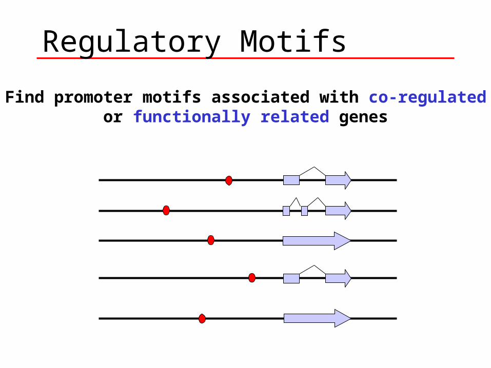
Regulatory Motifs

Find promoter motifs associated with co-regulated or functionally related genes

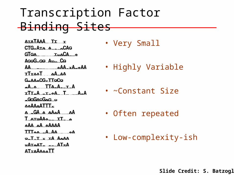
Transcription Factor Binding Sites

• Very Small

• Highly Variable

• ~Constant Size

• Often repeated

• Low-complexity-ish

Slide Credit: S. Batzoglou

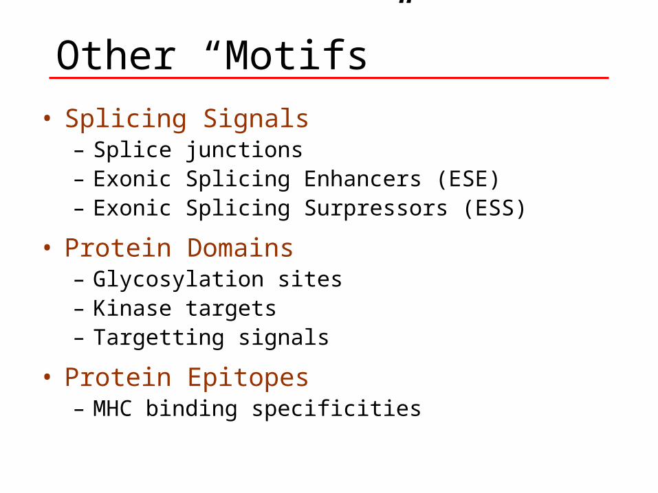
Other “Motifs”

• Splicing Signals– Splice junctions– Exonic Splicing Enhancers (ESE)– Exonic Splicing Surpressors (ESS)

• Protein Domains– Glycosylation sites– Kinase targets– Targetting signals

• Protein Epitopes– MHC binding specificities

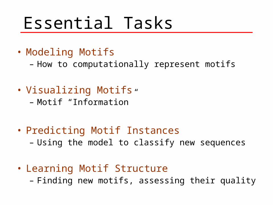
• Modeling Motifs– How to computationally represent motifs

• Visualizing Motifs– Motif “Information”

• Predicting Motif Instances– Using the model to classify new sequences

• Learning Motif Structure– Finding new motifs, assessing their quality

Essential Tasks

Modeling Motifs

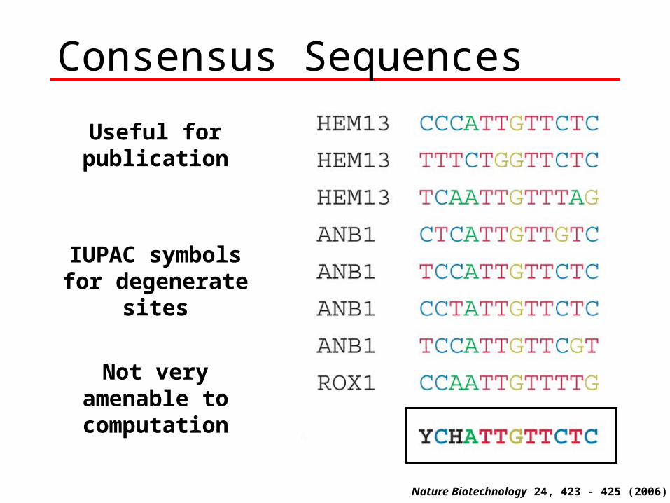
Consensus Sequences

Useful for publication

IUPAC symbols for degenerate

sites

Not very amenable to computation

Nature Biotechnology 24, 423 - 425 (2006)

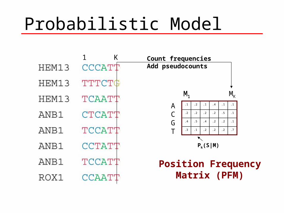
Probabilistic Model

.2

.2

.5

.1

.7.2.2.1.3

.1.2.4.5.4

.1.2.2.2.2

.1.4.1.2.1ACGT

M1 MKM1

Pk(S|M)

Position FrequencyMatrix (PFM)

1 K Count frequenciesAdd pseudocounts

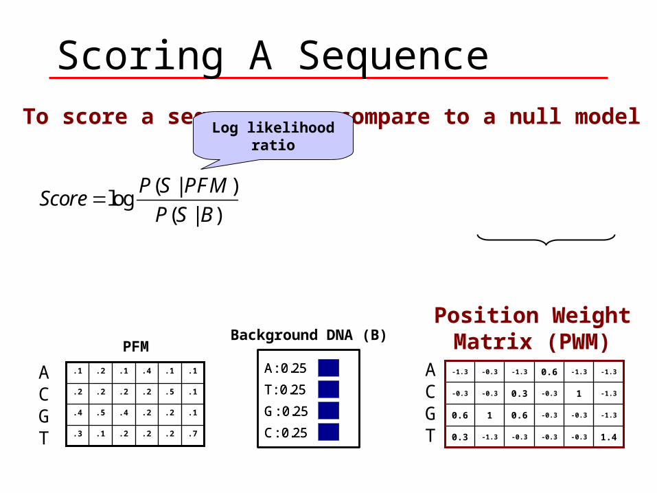
Scoring A Sequence

11

( | ) ( | )( | )log log log

( | ) ( | ) ( | )

N Ni i i i

ii i i

P S PFM P S PFMP S PFMScore

P S B P S B P S B

To score a sequence, we compare to a null model

A: 0.25

T: 0.25

G: 0.25

C: 0.25

A: 0.25

T: 0.25

G: 0.25

C: 0.25

Background DNA (B)

.2

.2

.5

.1

.7.2.2.1.3

.1.2.4.5.4

.1.2.2.2.2

.1.4.1.2.1ACGT

Log likelihoodratio

-0.3

-0.3

1

-1.3

1.4-0.3-0.3-1.30.3

-1.3-0.30.610.6

-1.3-0.30.3-0.3-0.3

-1.30.6-1.3-0.3-1.3ACGT

Position WeightMatrix (PWM)PFM

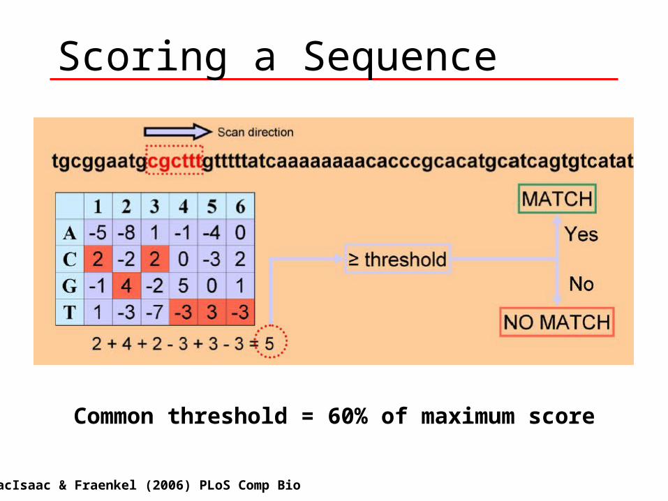
Scoring a Sequence

MacIsaac & Fraenkel (2006) PLoS Comp Bio

Common threshold = 60% of maximum score

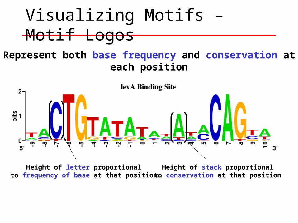
Visualizing Motifs – Motif Logos

Represent both base frequency and conservation at each position

Height of letter proportionalto frequency of base at that position

Height of stack proportionalto conservation at that position

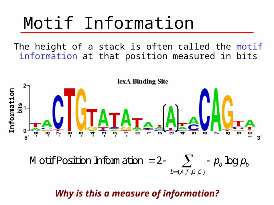
Motif InformationThe height of a stack is often called the motif information at

that position measured in bits

{ , , , }

Motif Position Information 2 logb bb A T G C

p p

Info

rmat

ion

Why is this a measure of information?

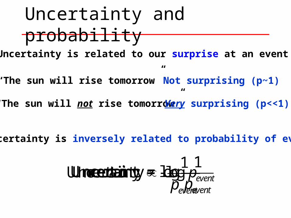
1Uncertainty = log

eventpUncertainty = - log eventp

1Uncertainty

eventp

Uncertainty and probability

“The sun will rise tomorrow”

“The sun will not rise tomorrow”

Uncertainty is inversely related to probability of event

Not surprising (p~1)

Very surprising (p<<1)

Uncertainty is related to our surprise at an event

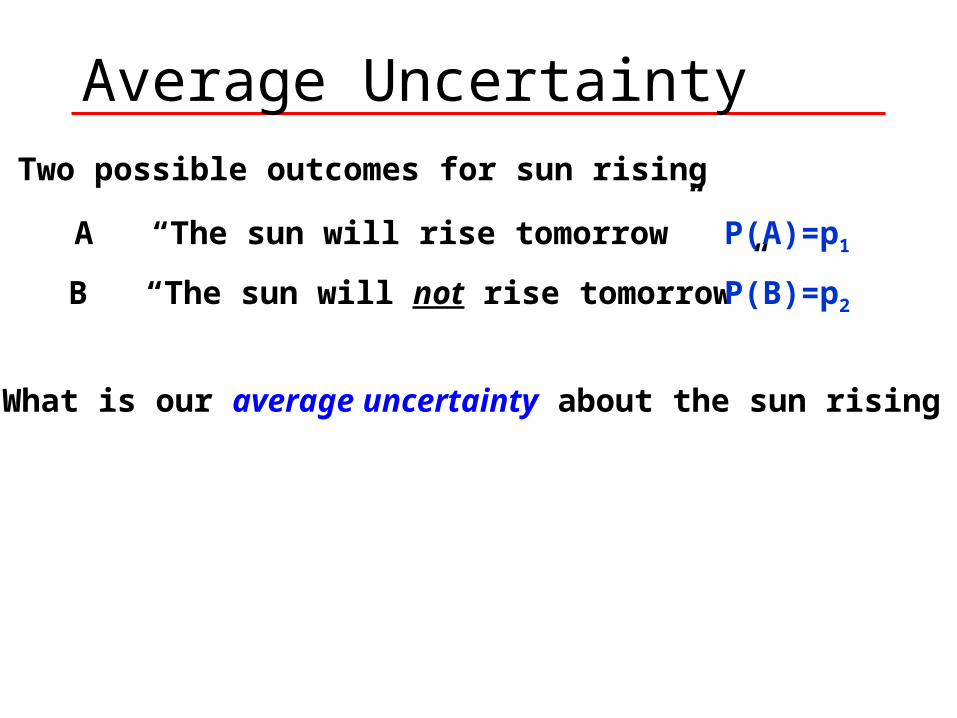
Average Uncertainty

A “The sun will rise tomorrow”

B “The sun will not rise tomorrow”

P(A)=p1

P(B)=p2

Two possible outcomes for sun rising

1 1 2 2

( )Uncertainty(A) ( )Uncertainty(B)

log log

logi i

P A P B

p p p p

p p

= Entropy

What is our average uncertainty about the sun rising

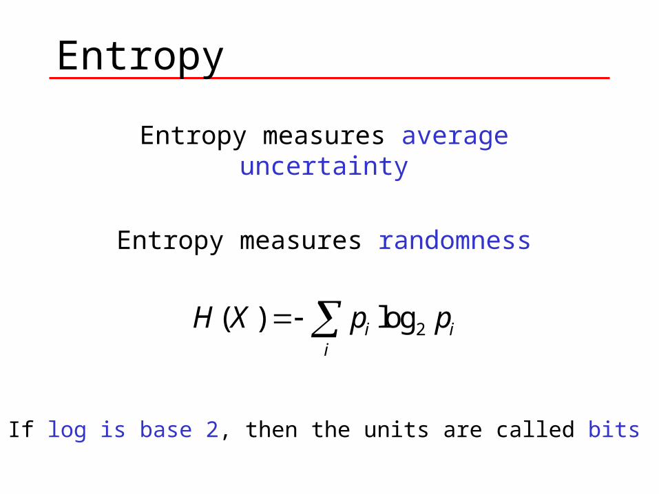
Entropy

Entropy measures average uncertainty

Entropy measures randomness

If log is base 2, then the units are called bits

2( ) logi ii

H X p p

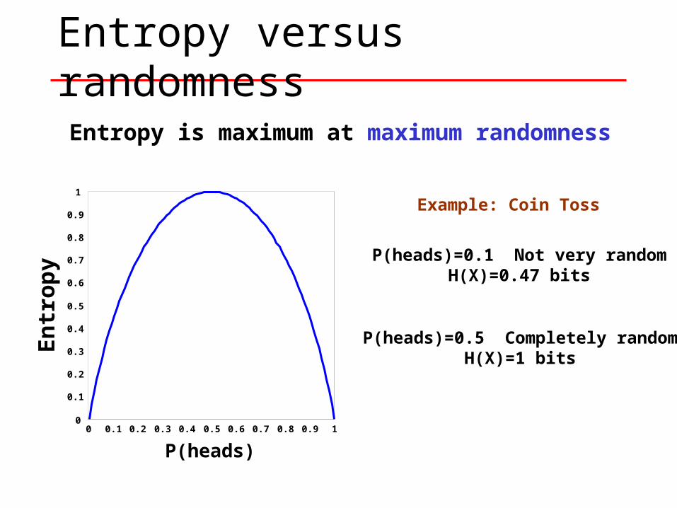
Entropy versus randomness

0 0.1 0.2 0.3 0.4 0.5 0.6 0.7 0.8 0.9 10

0.1

0.2

0.3

0.4

0.5

0.6

0.7

0.8

0.9

1

Entropy is maximum at maximum randomness

P(heads)

Example: Coin Toss

En

tro

py

P(heads)=0.1 Not very randomH(X)=0.47 bits

P(heads)=0.5 Completely randomH(X)=1 bits

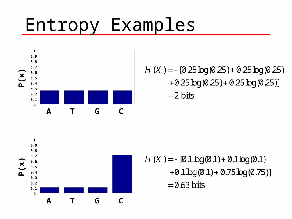
Entropy Examples

( ) [0.25log(0.25) 0.25log(0.25)

0.25log(0.25) 0.25log(0.25)]

2 bits

H X

1 2 3 40

0.1

0.2

0.3

0.4

0.5

0.6

0.7

0.8

0.9

1

P(x

)

0

0.1

0.2

0.3

0.4

0.5

0.6

0.7

0.8

0.9

1

1 2 3 4

P(x

) ( ) [0.1log(0.1) 0.1log(0.1)

0.1log(0.1) 0.75log(0.75)]

0.63 bits

H X

A T G C

A T G C

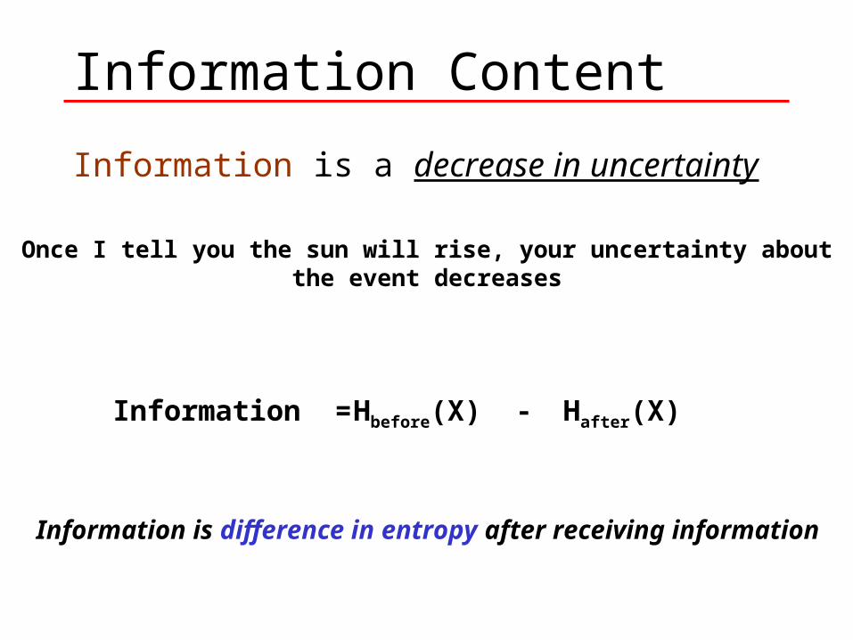
Information Content

Information is a decrease in uncertainty

Once I tell you the sun will rise, your uncertainty aboutthe event decreases

Hbefore(X) Hafter(X)-Information =

Information is difference in entropy after receiving information

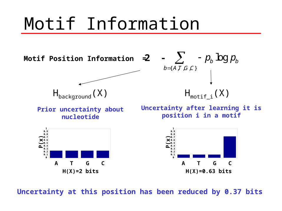
Motif Information

2 -Motif Position Information ={ , , , }

logb bb A T G C

p p

Hbackground(X) Hmotif_i(X)

Prior uncertainty aboutnucleotide

Uncertainty after learning it isposition i in a motif

H(X)=2 bits

A T G C0

0.10.20.30.40.50.60.70.80.9

1

P(x

)

H(X)=0.63 bits

A T G C0

0.10.20.30.40.50.60.70.80.9

1

P(x

)

Uncertainty at this position has been reduced by 0.37 bits

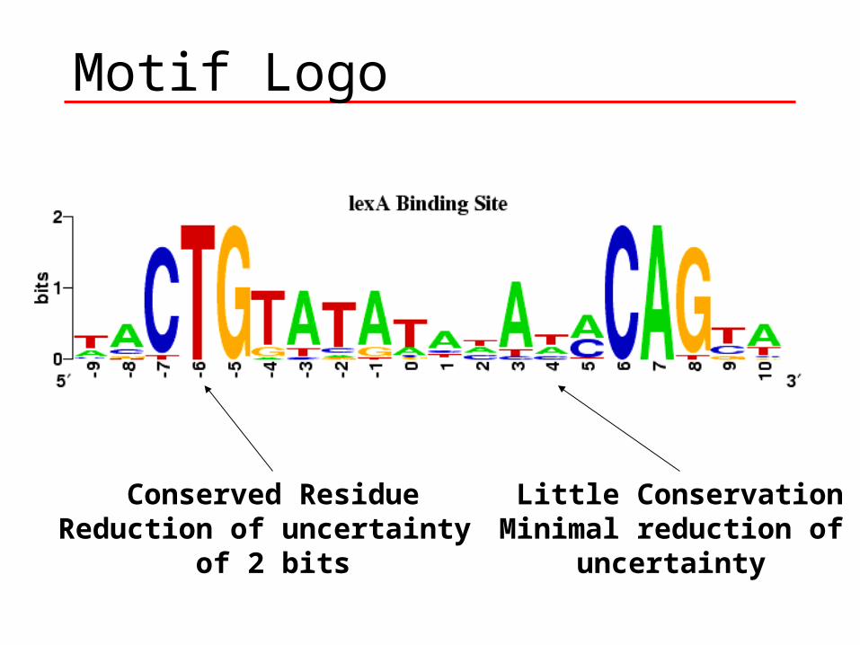
Motif Logo

Conserved ResidueReduction of uncertainty

of 2 bits

Little ConservationMinimal reduction of

uncertainty

{ , , , }

logb bb A T G C

p p

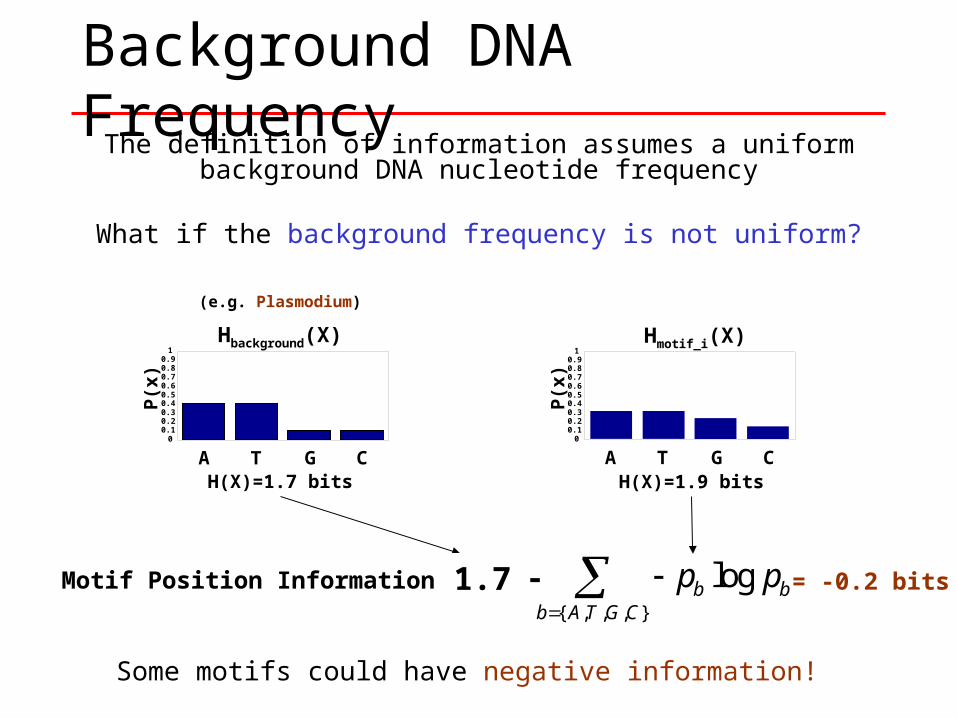
Background DNA Frequency

2 -Motif Position Information =

Hmotif_i(X)

H(X)=1.9 bitsA T G C

00.10.20.30.40.50.60.70.80.9

1

P(x

)

Some motifs could have negative information!

= -0.2 bits

The definition of information assumes a uniform background DNA nucleotide frequency

What if the background frequency is not uniform?

Hbackground(X)

H(X)=1.7 bitsA T G C

00.10.20.30.40.50.60.70.80.9

1

P(x

)

(e.g. Plasmodium)

1.7

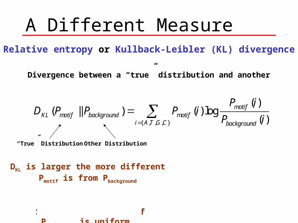
A Different MeasureRelative entropy or Kullback-Leibler (KL) divergence

Divergence between a “true” distribution and another

{ , , , }

( )( || ) ( ) log

( )motif

KL motif background motifi A T G C background

P iD P P P i

P i

“True” Distribution Other Distribution

DKL is larger the more differentPmotif is from Pbackground

Same as Information ifPbackground is uniform

Properties

motif backgroundif and only if P =P

0

0

( || ) ( || )

KL

KL

KL KL

D

D

D P Q D Q P

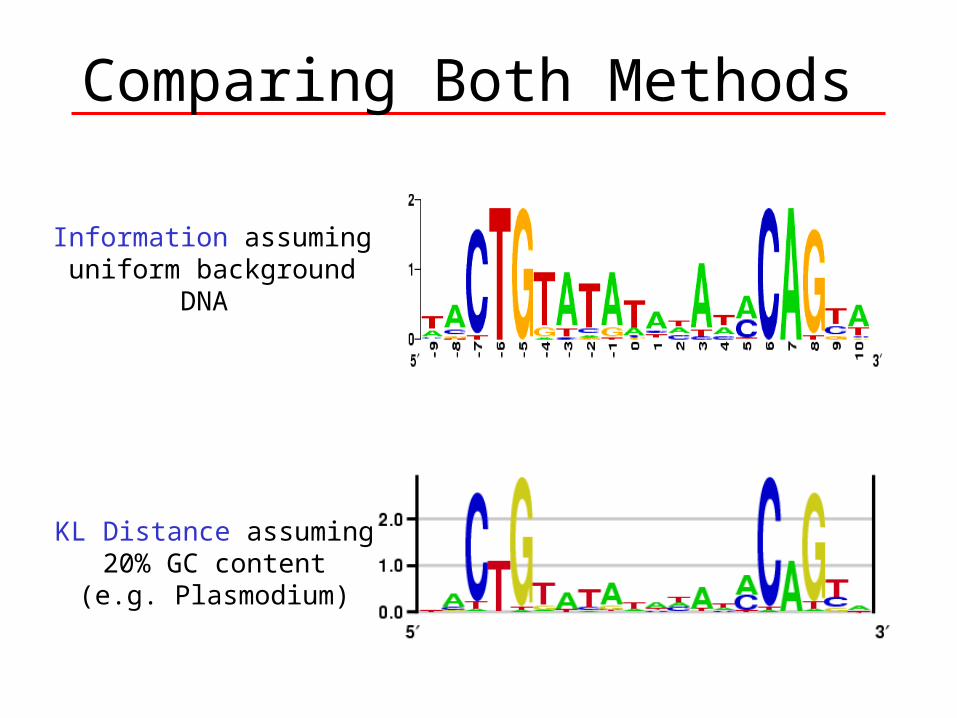
Comparing Both Methods

Information assuminguniform background

DNA

KL Distance assuming20% GC content

(e.g. Plasmodium)

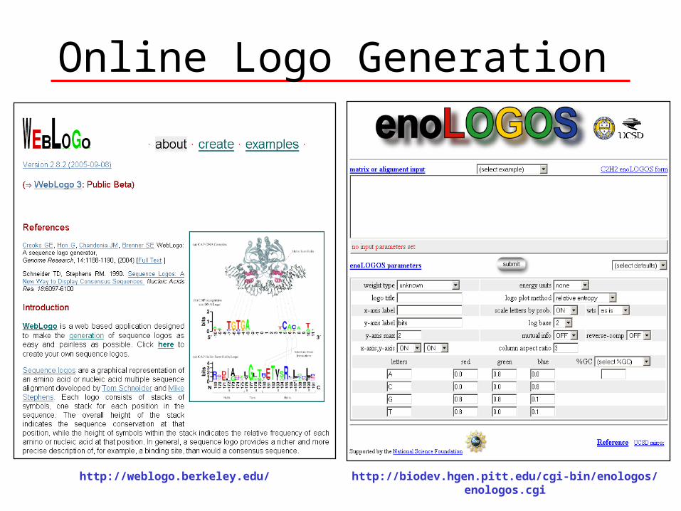
Online Logo Generation

http://weblogo.berkeley.edu/ http://biodev.hgen.pitt.edu/cgi-bin/enologos/enologos.cgi

Finding New Motifs

Learning Motif Models

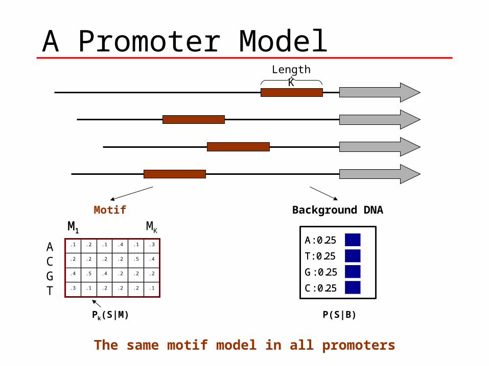
A Promoter ModelLength K

Motif

The same motif model in all promoters

.2

.2

.5

.1

.1.2.2.1.3

.2.2.4.5.4

.4.2.2.2.2

.3.4.1.2.1ACGT

M1 MKM1

Background DNA

A: 0.25

T: 0.25

G: 0.25

C: 0.25

A: 0.25

T: 0.25

G: 0.25

C: 0.25

P(S|B)Pk(S|M)

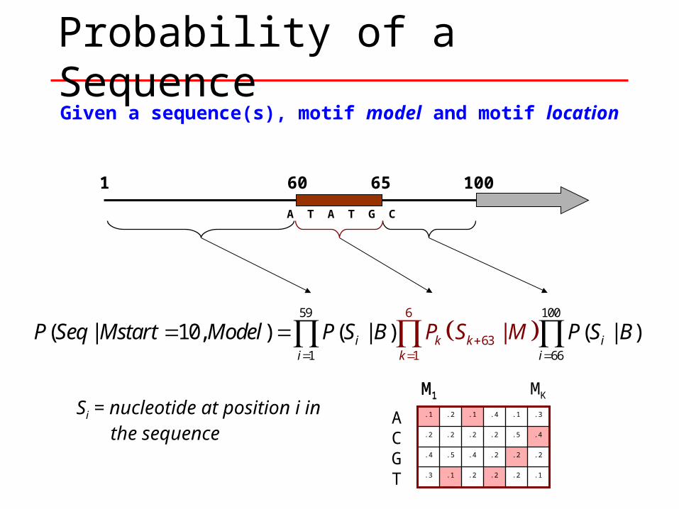
Probability of a Sequence

1 60 65 100

Given a sequence(s), motif model and motif location

59 6

631

100

1 66

|( | 10, ) ( | ) ( | )i ii

ki

kk

P Seq Mstart Model P S B PP SS M B

Si = nucleotide at position i in the sequence

A T A T G C

.2

.2

.5

.1

.1.2.2.1.3

.2.2.4.5.4

.4.2.2.2.2

.3.4.1.2.1ACGT

M1 MKM1

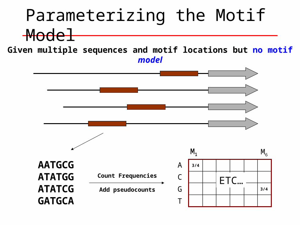
Parameterizing the Motif ModelGiven multiple sequences and motif locations but no motif model

A

C

G

T

M1 M6M1

3/4

3/4

ETC…

AATGCGATATGGATATCGGATGCA

Count Frequencies

Add pseudocounts

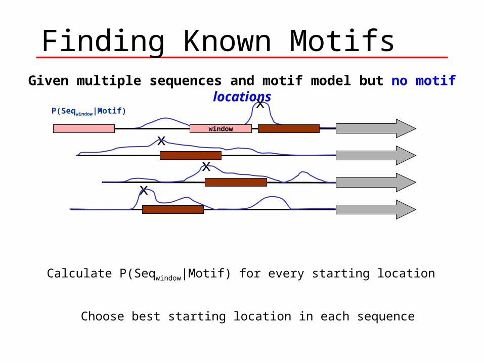
Finding Known MotifsGiven multiple sequences and motif model but no motif locations

x

x

x

xP(Seqwindow|Motif)

window

Calculate P(Seqwindow|Motif) for every starting location

Choose best starting location in each sequence

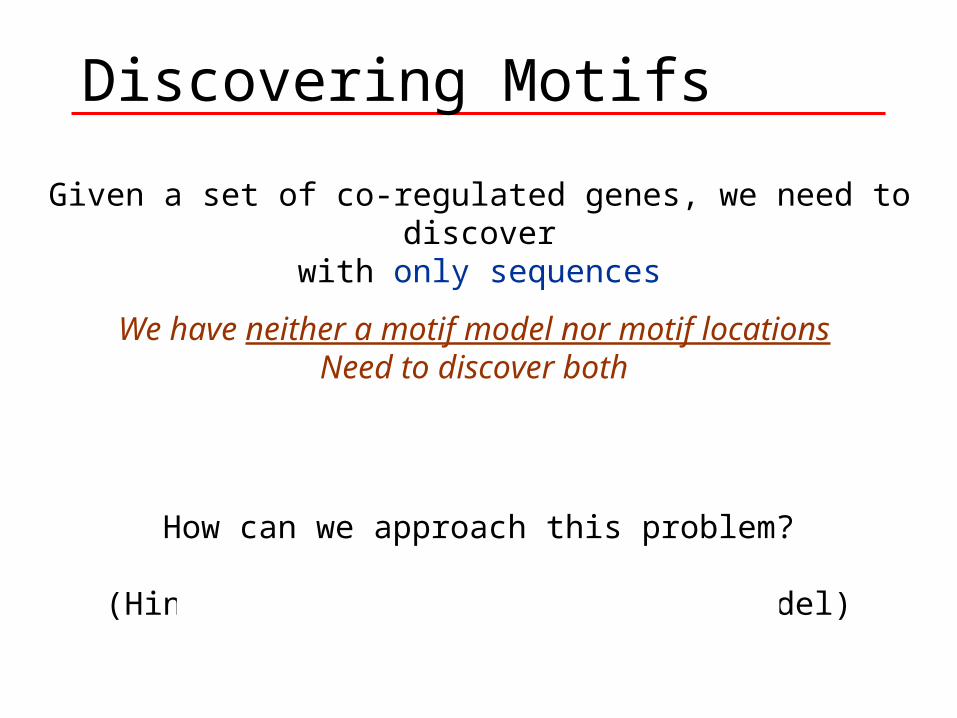
Discovering Motifs

Given a set of co-regulated genes, we need to discoverwith only sequences

We have neither a motif model nor motif locationsNeed to discover both

How can we approach this problem?

(Hint: start with a random motif model)

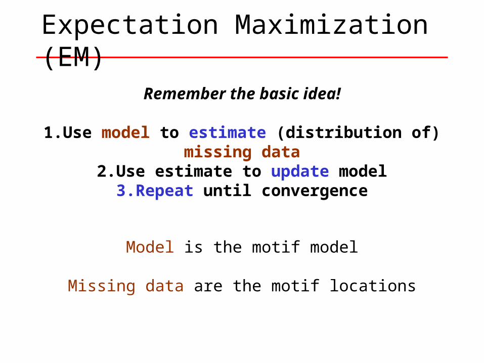
Expectation Maximization (EM)

Remember the basic idea!

1.Use model to estimate (distribution of) missing data2.Use estimate to update model

3.Repeat until convergence

Model is the motif model

Missing data are the motif locations

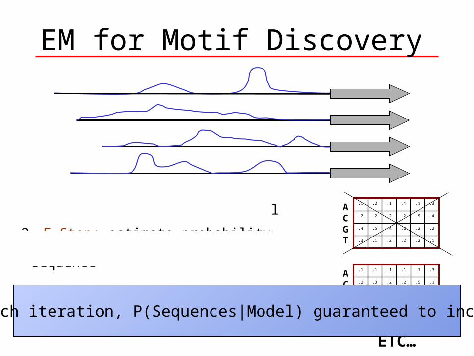
EM for Motif Discovery

1. Start with random motif model

2. E Step: estimate probability of motif positions for each sequence

3. M Step: use estimate to update motif model

4. Iterate (to convergence)

.2

.2

.5

.1

.1.2.2.1.3

.2.2.4.5.4

.4.2.2.2.2

.3.4.1.2.1ACGT

.2

.2

.5

.1

.1.2.2.1.3

.1.5.4.5.4

.1.2.2.3.2

.3.1.1.1.1ACGT

ETC…

At each iteration, P(Sequences|Model) guaranteed to increase

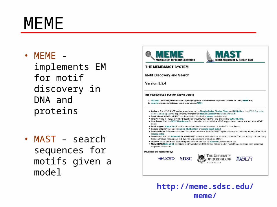
MEME

http://meme.sdsc.edu/meme/

• MEME - implements EM for motif discovery in DNA and proteins

• MAST – search sequences for motifs given a model

P(Seq|Model) Landscape

P(S

eq

ue

nc

es

|pa

ram

s1

,pa

ram

s2

)

EM searches for parameters to increase P(seqs|parameters)

Useful to think of P(seqs|parameters)

as a function of parameters

Parameter1 Parameter2

EM starts at an initial set ofparameters

And then “climbs uphill” until it reaches a local maximum

Where EM starts can make a big difference

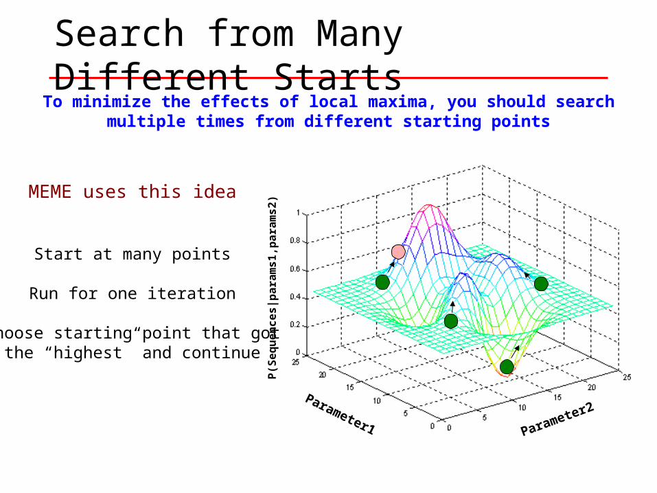
Search from Many Different Starts

P(S

eq

ue

nc

es

|pa

ram

s1

,pa

ram

s2

)

To minimize the effects of local maxima, you should searchmultiple times from different starting points

Parameter1 Parameter2

MEME uses this idea

Start at many points

Run for one iteration

Choose starting point that gotthe “highest” and continue

Gibbs Sampling

A stochastic version of EM that differs from deterministic EM in two key ways

1. At each iteration, we only update the motif positionof a single sequence

2. We may update a motif position to a “suboptimal” new position

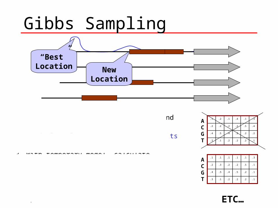
1. Start with random motif locations and calculate a motif model

2. Randomly select a sequence, remove its motif and recalculate tempory model

3. With temporary model, calculate probability of motif at each position on sequence

4. Select new position based on this distribution

5. Update model and Iterate

Gibbs Sampling

.2

.2

.5

.1

.1.2.2.1.3

.2.2.4.5.4

.4.2.2.2.2

.3.4.1.2.1ACGT

.2

.2

.5

.1

.1.2.2.1.3

.1.5.4.5.4

.1.2.2.3.2

.3.1.1.1.1ACGT

ETC…

“Best”Location New

Location

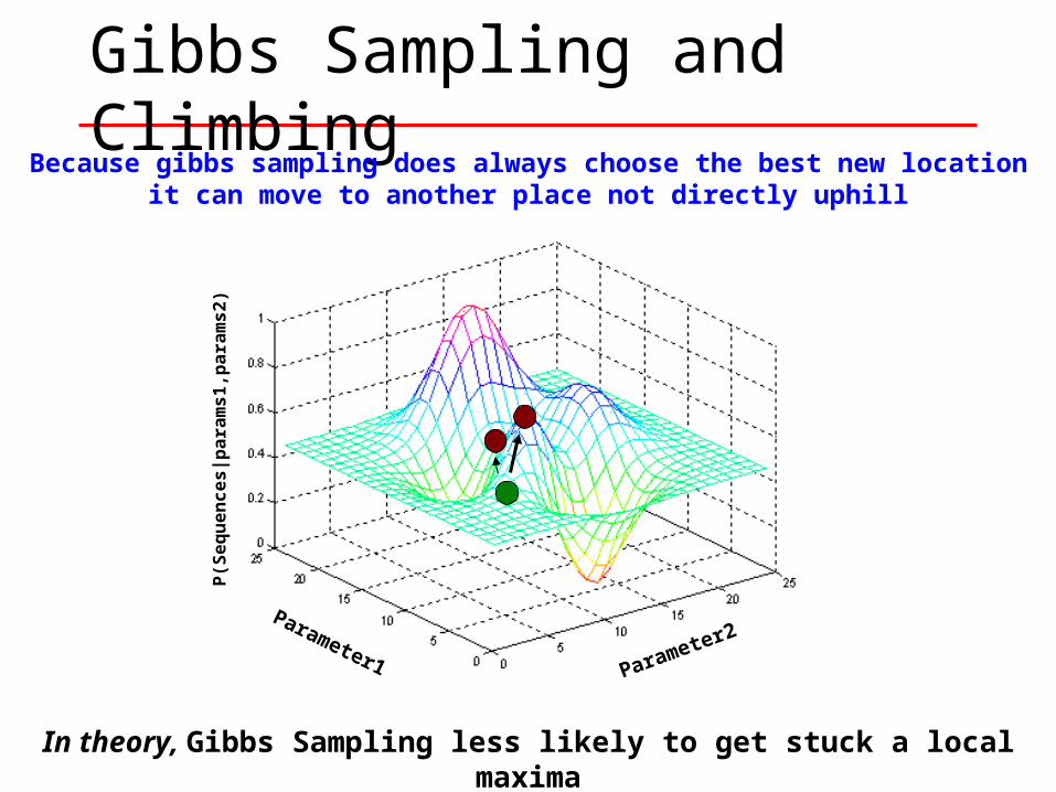
Gibbs Sampling and Climbing

P(S

eq

ue

nc

es

|pa

ram

s1

,pa

ram

s2

)

Because gibbs sampling does always choose the best new locationit can move to another place not directly uphill

Parameter1 Parameter2

In theory, Gibbs Sampling less likely to get stuck a local maxima

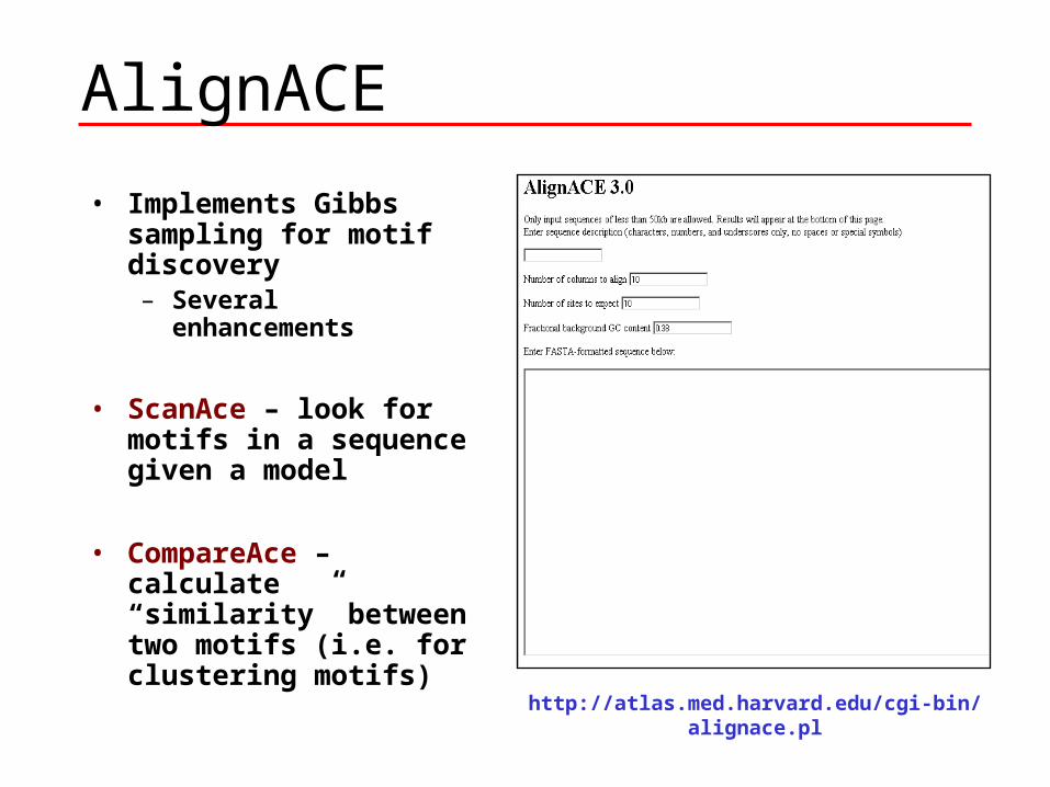
AlignACE

http://atlas.med.harvard.edu/cgi-bin/alignace.pl

• Implements Gibbs sampling for motif discovery– Several enhancements

• ScanAce – look for motifs in a sequence given a model

• CompareAce – calculate “similarity” between two motifs (i.e. for clustering motifs)

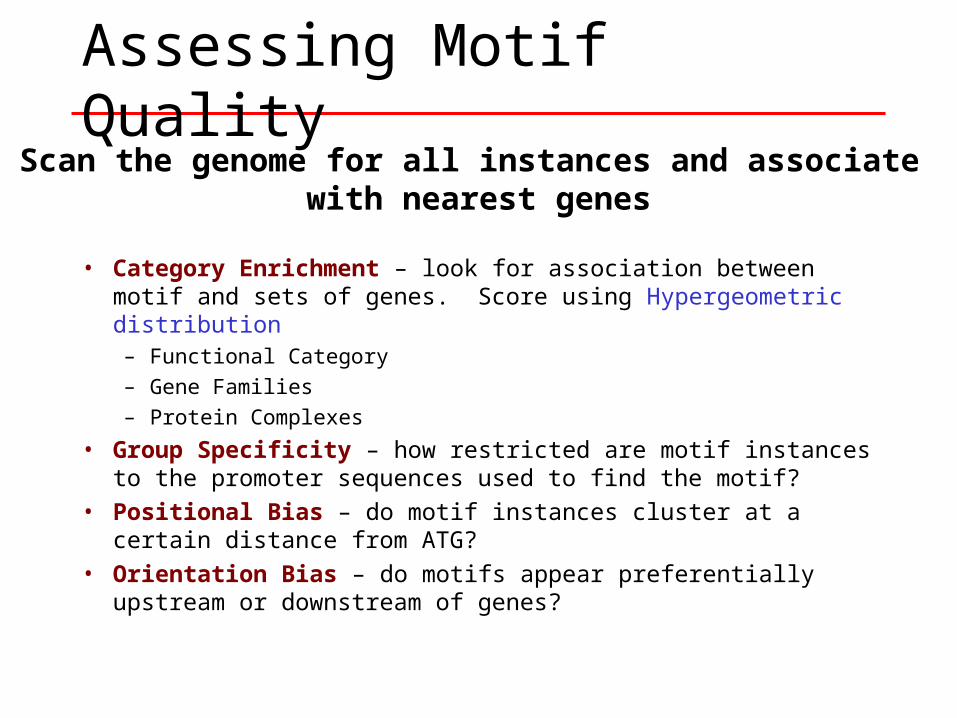
Assessing Motif QualityScan the genome for all instances and associate

with nearest genes

• Category Enrichment – look for association between motif and sets of genes. Score using Hypergeometric distribution– Functional Category

– Gene Families

– Protein Complexes

• Group Specificity – how restricted are motif instances to the promoter sequences used to find the motif?

• Positional Bias – do motif instances cluster at a certain distance from ATG?

• Orientation Bias – do motifs appear preferentially upstream or downstream of genes?

Comparative Motif Prediction

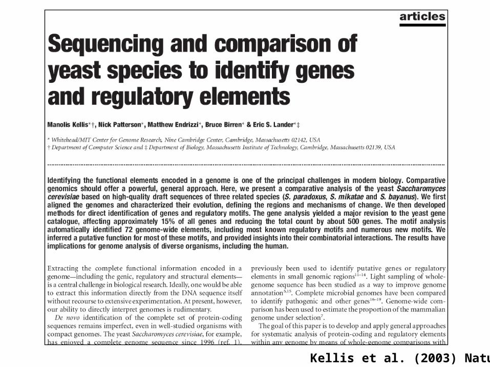
Kellis et al. (2003) Nature

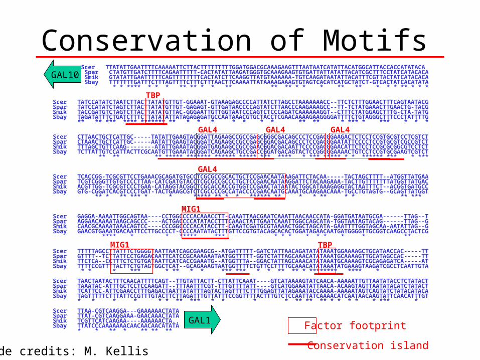
Scer TTATATTGAATTTTCAAAAATTCTTACTTTTTTTTTGGATGGACGCAAAGAAGTTTAATAATCATATTACATGGCATTACCACCATATACA Spar CTATGTTGATCTTTTCAGAATTTTT-CACTATATTAAGATGGGTGCAAAGAAGTGTGATTATTATATTACATCGCTTTCCTATCATACACA Smik GTATATTGAATTTTTCAGTTTTTTTTCACTATCTTCAAGGTTATGTAAAAAA-TGTCAAGATAATATTACATTTCGTTACTATCATACACA Sbay TTTTTTTGATTTCTTTAGTTTTCTTTCTTTAACTTCAAAATTATAAAAGAAAGTGTAGTCACATCATGCTATCT-GTCACTATCACATATA * * **** * * * ** ** * * ** ** ** * * * ** ** * * * ** * * *

Scer TATCCATATCTAATCTTACTTATATGTTGT-GGAAAT-GTAAAGAGCCCCATTATCTTAGCCTAAAAAAACC--TTCTCTTTGGAACTTTCAGTAATACGSpar TATCCATATCTAGTCTTACTTATATGTTGT-GAGAGT-GTTGATAACCCCAGTATCTTAACCCAAGAAAGCC--TT-TCTATGAAACTTGAACTG-TACGSmik TACCGATGTCTAGTCTTACTTATATGTTAC-GGGAATTGTTGGTAATCCCAGTCTCCCAGATCAAAAAAGGT--CTTTCTATGGAGCTTTG-CTA-TATGSbay TAGATATTTCTGATCTTTCTTATATATTATAGAGAGATGCCAATAAACGTGCTACCTCGAACAAAAGAAGGGGATTTTCTGTAGGGCTTTCCCTATTTTG ** ** *** **** ******* ** * * * * * * * ** ** * *** * *** * * *

Scer CTTAACTGCTCATTGC-----TATATTGAAGTACGGATTAGAAGCCGCCGAGCGGGCGACAGCCCTCCGACGGAAGACTCTCCTCCGTGCGTCCTCGTCTSpar CTAAACTGCTCATTGC-----AATATTGAAGTACGGATCAGAAGCCGCCGAGCGGACGACAGCCCTCCGACGGAATATTCCCCTCCGTGCGTCGCCGTCTSmik TTTAGCTGTTCAAG--------ATATTGAAATACGGATGAGAAGCCGCCGAACGGACGACAATTCCCCGACGGAACATTCTCCTCCGCGCGGCGTCCTCTSbay TCTTATTGTCCATTACTTCGCAATGTTGAAATACGGATCAGAAGCTGCCGACCGGATGACAGTACTCCGGCGGAAAACTGTCCTCCGTGCGAAGTCGTCT ** ** ** ***** ******* ****** ***** *** **** * *** ***** * * ****** *** * ***

Scer TCACCGG-TCGCGTTCCTGAAACGCAGATGTGCCTCGCGCCGCACTGCTCCGAACAATAAAGATTCTACAA-----TACTAGCTTTT--ATGGTTATGAASpar TCGTCGGGTTGTGTCCCTTAA-CATCGATGTACCTCGCGCCGCCCTGCTCCGAACAATAAGGATTCTACAAGAAA-TACTTGTTTTTTTATGGTTATGACSmik ACGTTGG-TCGCGTCCCTGAA-CATAGGTACGGCTCGCACCACCGTGGTCCGAACTATAATACTGGCATAAAGAGGTACTAATTTCT--ACGGTGATGCCSbay GTG-CGGATCACGTCCCTGAT-TACTGAAGCGTCTCGCCCCGCCATACCCCGAACAATGCAAATGCAAGAACAAA-TGCCTGTAGTG--GCAGTTATGGT ** * ** *** * * ***** ** * * ****** ** * * ** * * ** ***

Scer GAGGA-AAAATTGGCAGTAA----CCTGGCCCCACAAACCTT-CAAATTAACGAATCAAATTAACAACCATA-GGATGATAATGCGA------TTAG--TSpar AGGAACAAAATAAGCAGCCC----ACTGACCCCATATACCTTTCAAACTATTGAATCAAATTGGCCAGCATA-TGGTAATAGTACAG------TTAG--GSmik CAACGCAAAATAAACAGTCC----CCCGGCCCCACATACCTT-CAAATCGATGCGTAAAACTGGCTAGCATA-GAATTTTGGTAGCAA-AATATTAG--GSbay GAACGTGAAATGACAATTCCTTGCCCCT-CCCCAATATACTTTGTTCCGTGTACAGCACACTGGATAGAACAATGATGGGGTTGCGGTCAAGCCTACTCG **** * * ***** *** * * * * * * * * **

Scer TTTTTAGCCTTATTTCTGGGGTAATTAATCAGCGAAGCG--ATGATTTTT-GATCTATTAACAGATATATAAATGGAAAAGCTGCATAACCAC-----TTSpar GTTTT--TCTTATTCCTGAGACAATTCATCCGCAAAAAATAATGGTTTTT-GGTCTATTAGCAAACATATAAATGCAAAAGTTGCATAGCCAC-----TTSmik TTCTCA--CCTTTCTCTGTGATAATTCATCACCGAAATG--ATGGTTTA--GGACTATTAGCAAACATATAAATGCAAAAGTCGCAGAGATCA-----ATSbay TTTTCCGTTTTACTTCTGTAGTGGCTCAT--GCAGAAAGTAATGGTTTTCTGTTCCTTTTGCAAACATATAAATATGAAAGTAAGATCGCCTCAATTGTA * * * *** * ** * * *** *** * * ** ** * ******** **** *

Scer TAACTAATACTTTCAACATTTTCAGT--TTGTATTACTT-CTTATTCAAAT----GTCATAAAAGTATCAACA-AAAAATTGTTAATATACCTCTATACTSpar TAAATAC-ATTTGCTCCTCCAAGATT--TTTAATTTCGT-TTTGTTTTATT----GTCATGGAAATATTAACA-ACAAGTAGTTAATATACATCTATACTSmik TCATTCC-ATTCGAACCTTTGAGACTAATTATATTTAGTACTAGTTTTCTTTGGAGTTATAGAAATACCAAAA-AAAAATAGTCAGTATCTATACATACASbay TAGTTTTTCTTTATTCCGTTTGTACTTCTTAGATTTGTTATTTCCGGTTTTACTTTGTCTCCAATTATCAAAACATCAATAACAAGTATTCAACATTTGT * * * * * * ** *** * * * * ** ** ** * * * * * *** *

Scer TTAA-CGTCAAGGA---GAAAAAACTATASpar TTAT-CGTCAAGGAAA-GAACAAACTATASmik TCGTTCATCAAGAA----AAAAAACTA..Sbay TTATCCCAAAAAAACAACAACAACATATA * * ** * ** ** **

GAL10

GAL1

TBP

GAL4 GAL4 GAL4

GAL4

MIG1

TBPMIG1

Factor footprint

Conservation islandslide credits: M. Kellis

Conservation of Motifs

Spar

Smik

Sbay

Scer

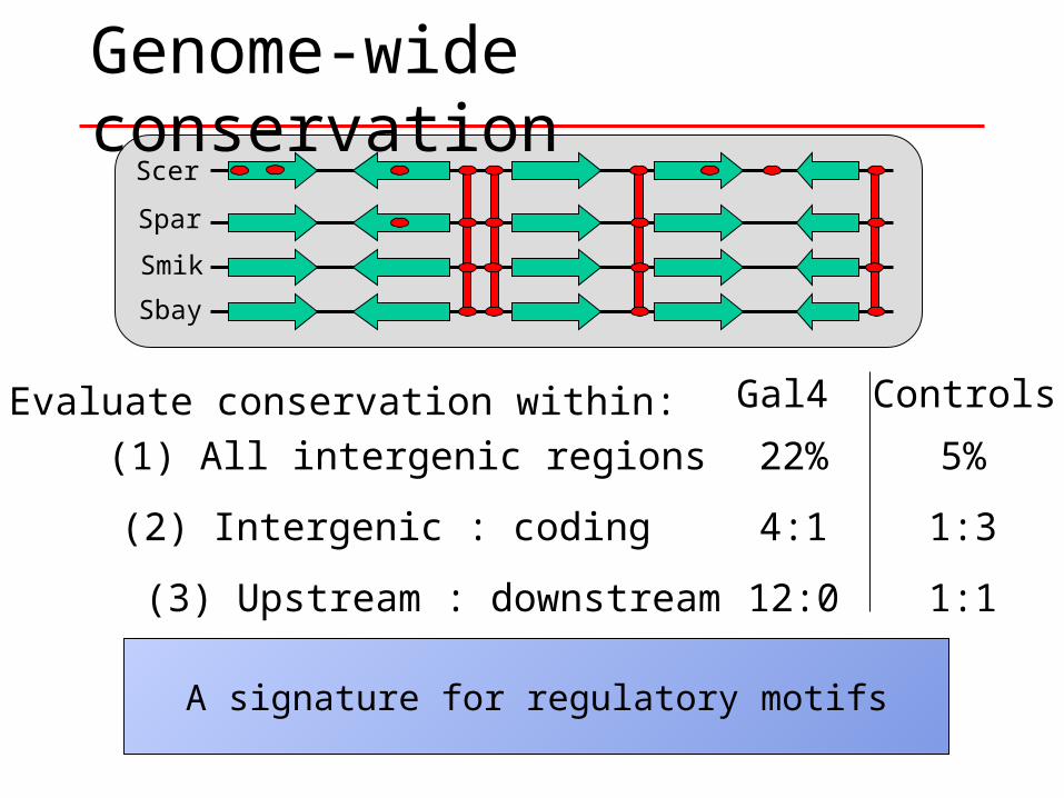
Evaluate conservation within: Gal4 Controls

4:1 1:3(2) Intergenic : coding

12:0 1:1(3) Upstream : downstream

A signature for regulatory motifs

22% 5%(1) All intergenic regions

Genome-wide conservation

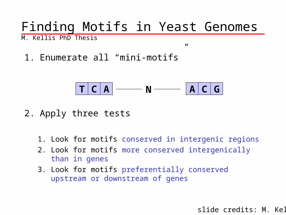
1. Enumerate all “mini-motifs”

2. Apply three tests

1. Look for motifs conserved in intergenic regions

2. Look for motifs more conserved intergenically than in genes

3. Look for motifs preferentially conserved upstream or downstream of genes

CT A C GAN

slide credits: M. Kellis

Finding Motifs in Yeast GenomesM. Kellis PhD Thesis

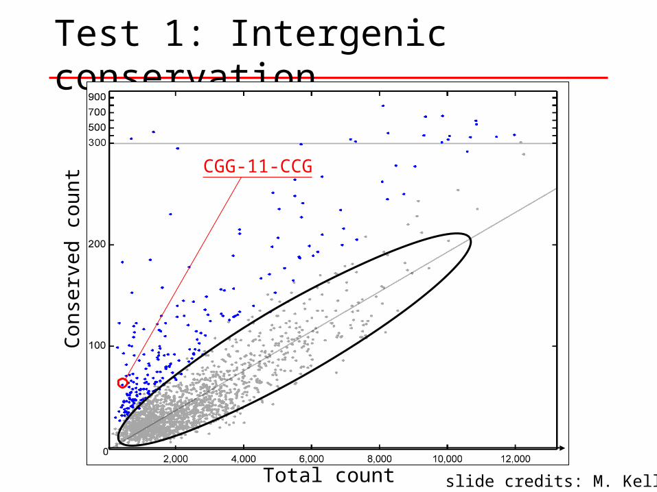
Test 1: Intergenic conservation

Total count

Con

serv

ed c

ount

CGG-11-CCG

slide credits: M. Kellis

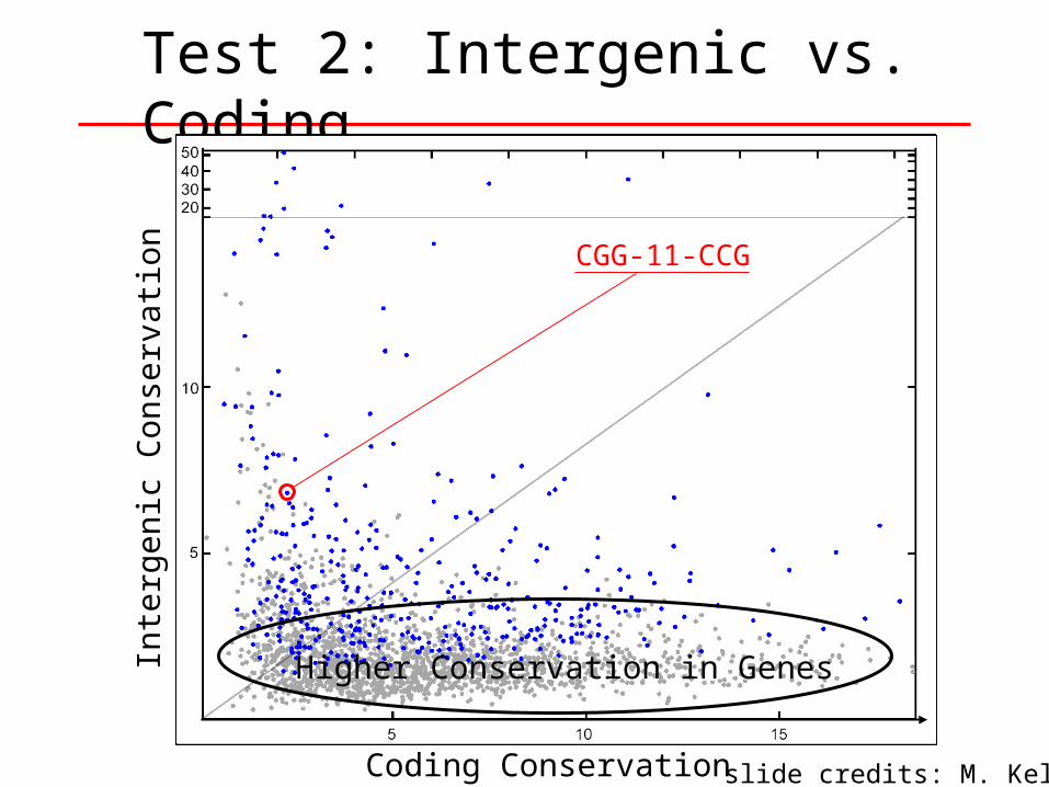
Test 2: Intergenic vs. Coding

Coding Conservation

Inte

rgen

ic C

onse

rvat

ion

CGG-11-CCG

Higher Conservation in Genes

slide credits: M. Kellis

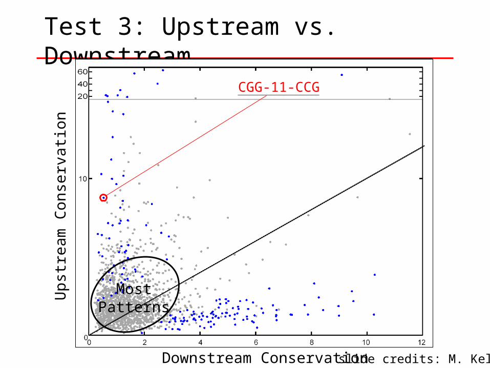
Test 3: Upstream vs. Downstream

CGG-11-CCG

MostPatterns

Downstream Conservation

Ups

trea

m C

onse

rvat

ion

slide credits: M. Kellis

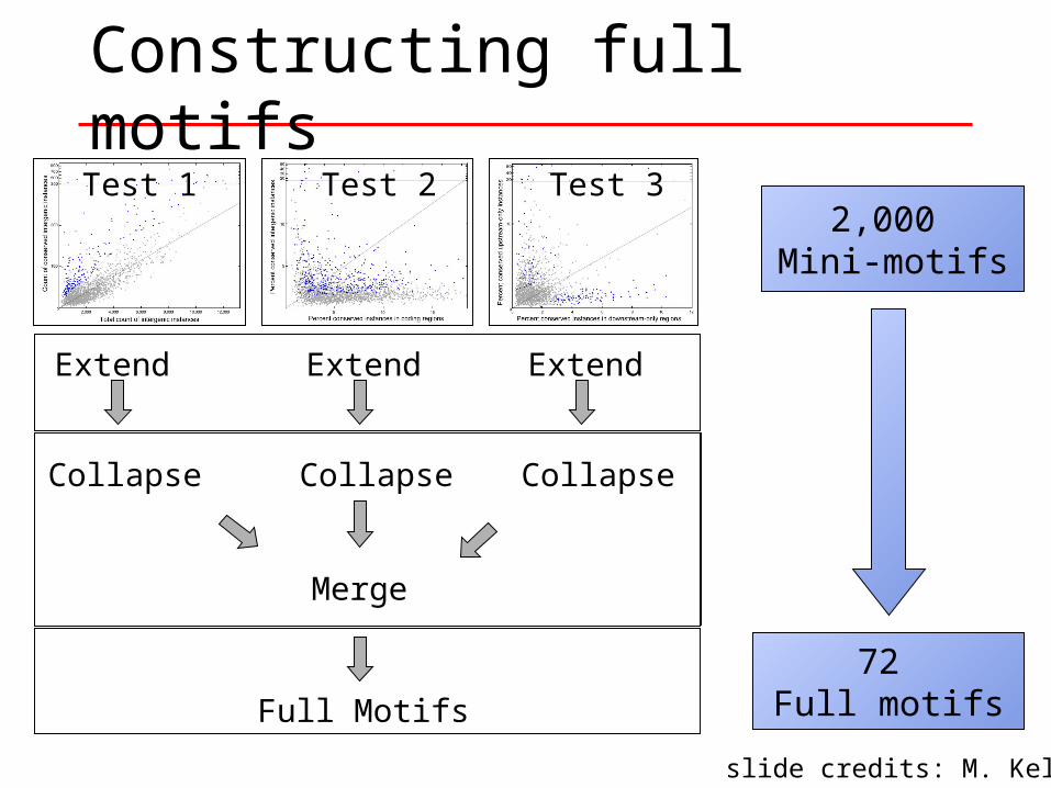
Extend

Collapse

Full Motifs

Constructing full motifs

2,000 Mini-motifs

72 Full motifs

6CT A C GAR R

CT GR C C GA AA CCTG C GA A

CT GR C C GA ACT RA Y C GA A

Y 5Extend Extend Extend

Collapse Collapse Collapse

Merge

Test 1 Test 2 Test 3

slide credits: M. Kellis

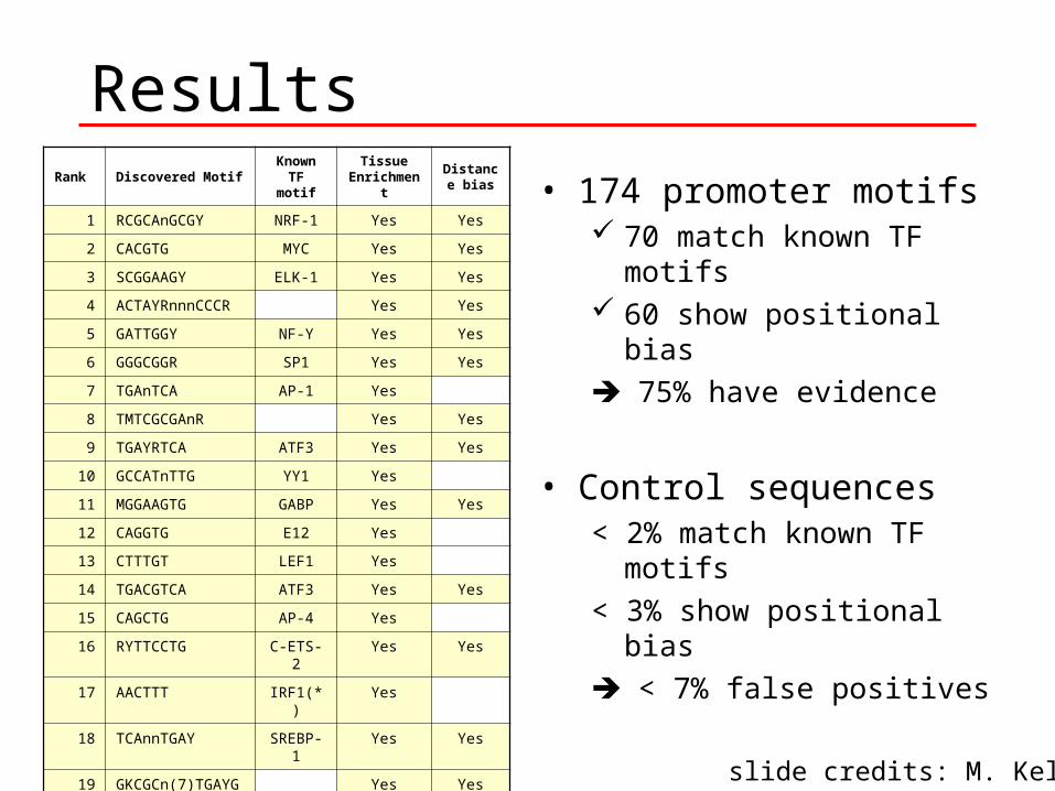
Rank Discovered MotifKnown

TF motifTissue

EnrichmentDistance

bias

1 RCGCAnGCGY NRF-1 Yes Yes

2 CACGTG MYC Yes Yes

3 SCGGAAGY ELK-1 Yes Yes

4 ACTAYRnnnCCCR Yes Yes

5 GATTGGY NF-Y Yes Yes

6 GGGCGGR SP1 Yes Yes

7 TGAnTCA AP-1 Yes

8 TMTCGCGAnR Yes Yes

9 TGAYRTCA ATF3 Yes Yes

10 GCCATnTTG YY1 Yes

11 MGGAAGTG GABP Yes Yes

12 CAGGTG E12 Yes

13 CTTTGT LEF1 Yes

14 TGACGTCA ATF3 Yes Yes

15 CAGCTG AP-4 Yes

16 RYTTCCTG C-ETS-2 Yes Yes

17 AACTTT IRF1(*) Yes

18 TCAnnTGAY SREBP-1

Yes Yes

19 GKCGCn(7)TGAYG

Yes Yes

• 174 promoter motifs 70 match known TF motifs 60 show positional bias

75% have evidence

• Control sequences< 2% match known TF motifs

< 3% show positional bias

< 7% false positives

slide credits: M. Kellis

Results

Antigen Epitope Prediction

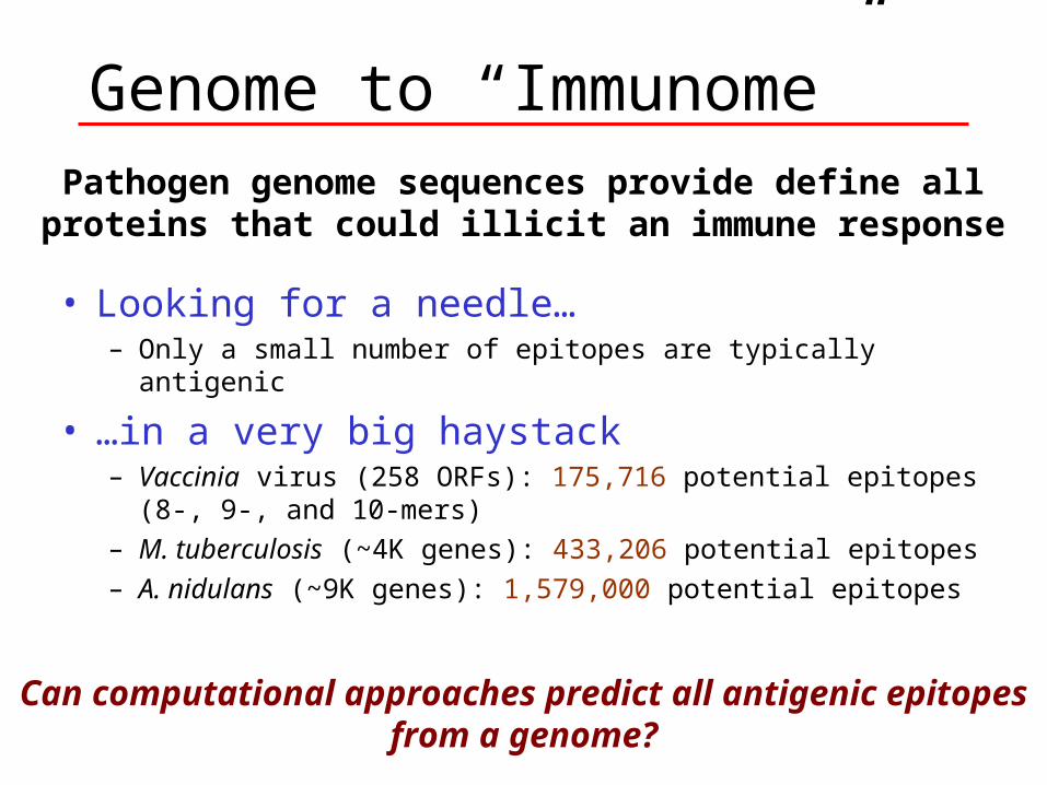
Genome to “Immunome”

• Looking for a needle…– Only a small number of epitopes are typically antigenic

• …in a very big haystack– Vaccinia virus (258 ORFs): 175,716 potential epitopes (8-, 9-,

and 10-mers)– M. tuberculosis (~4K genes): 433,206 potential epitopes – A. nidulans (~9K genes): 1,579,000 potential epitopes

Can computational approaches predict all antigenic epitopes from a genome?

Pathogen genome sequences provide define all proteins that could illicit an immune response

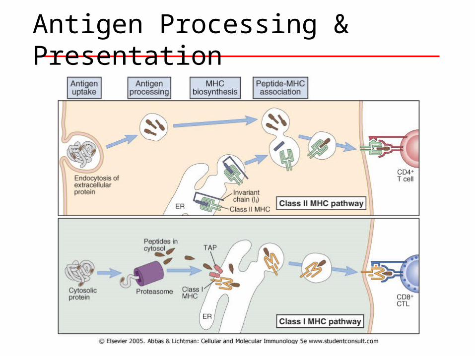
Antigen Processing & Presentation

Modeling MHC Epitopes

• Have a set of peptides that have been associate with a particular MHC allele

• Want to discover motif within the peptide bound by MHC allele

• Use motif to predict other potential epitopes

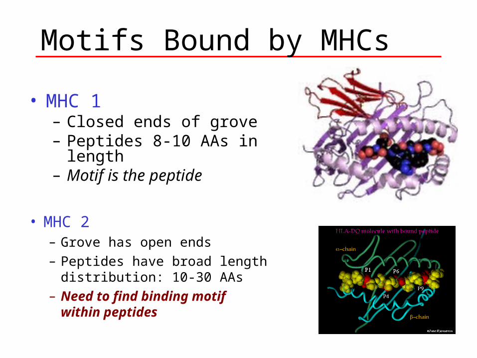
Motifs Bound by MHCs

• MHC 1– Closed ends of grove– Peptides 8-10 AAs in length– Motif is the peptide

• MHC 2– Grove has open ends– Peptides have broad length

distribution: 10-30 AAs– Need to find binding motif

within peptides

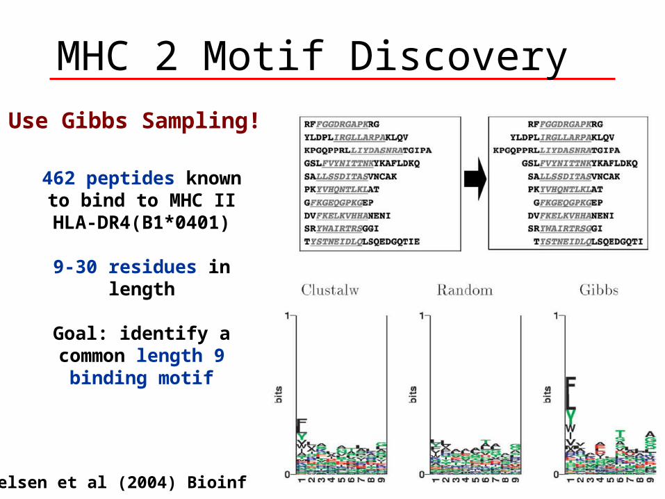
MHC 2 Motif Discovery

Nielsen et al (2004) Bioinf

Use Gibbs Sampling!

462 peptides known to bind to MHC II

HLA-DR4(B1*0401)

9-30 residues in length

Goal: identify a common length 9 binding motif

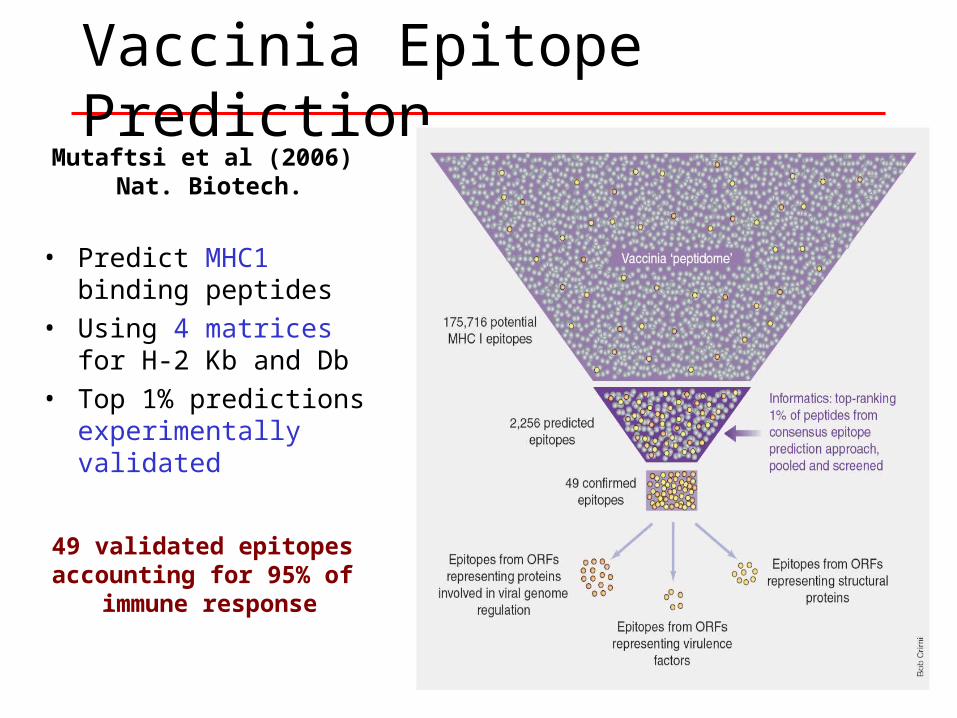
Vaccinia Epitope PredictionMutaftsi et al (2006)

Nat. Biotech.

• Predict MHC1 binding peptides

• Using 4 matrices for H-2 Kb and Db

• Top 1% predictions experimentally validated

49 validated epitopes accounting for 95% of

immune response