biological networks - web.cs.ucdavis.edu

Filkov, ECS289A, S05

Biological Networks

• Gene Networks

• Metabolic Networks

• Signaling Pathways

• Others …

• Modeling

• Inference


Simple Genetic Circuits

McAdams and Arkin et al 1998


Cis-regulatory input

of lacZYA operon in E. coli

Setty et al. PNAS 2003


Li, Fangting et al. (2004) Proc. Natl. Acad. Sci.

Cell cycle network in S.

Cerevisiae


Segment polarity

network in Drosophila

Nodes: mRNA (round), protein (rectangle), prot. Complex (octagon)

Edges: biochemical interactions or regulatory relationships

Albert and Otmer, JTB 2003


Gene network of endomeso

development in Sea Urchin

Davidson et al. Science 2002


Logic of Cis-regulation


Transcriptional

Regulatory Systems

• Cis regulatory elements: DNA sequence (specific sites)

• promoters;

• enhancers;

• silencers;

• Trans regulatory factors: products of regulatory genes

• generalized

• specific (Zinc finger, leucine zipper, etc.)

Known properties of real gene regulatory systems:

• cis-trans specificity

• small number of trans factors to a cis element: 8-10

• cis elements are programs

• regulation is event driven (asynchronous)

• regulation systems are noisy environments

• Protein-DNA and protein-protein regulation

• regulation changes with time


Gene Regulatory

Networks

Gene Networks: models of measurable

properties of Gene Regulatory

Systems.

Gene networks model functional

elements of a Gene Regulation System

together with the regulatory relationships

among them in a computational

formalism.

Types of relationships: causal, binding

specificity, protein-DNA binding, protein-

protein binding, etc.


Modeling Formalisms

• Static Graph

Models

• Boolean Networks

• Weight Matrix

(Linear) Models

• Bayesian Networks

• Stochastic Models

• Difference /

Differential Equation

Models

• Chemical/Physical

Models

• Concurrency models

Combinatorial

(Qualitative)

Physical

(Quantitative or

Continuous)


Continuous Models of

Gene Regulation


Outline

• Quantitative Modeling

• Discrete vs. Continuous

• Modeling problems

• Models:

– ODE

– PDE

– Stochastic

• Conclusions


Quantitative Modeling

in Biology

• State variables: concentrations of

substances, e.g. proteins, mRNA,

small molecules, etc.

• Knowing a system means being able

to predict the concentrations of all

key substances (state variables)

• Quantitative Modeling is the process

of connecting the components of a

system in a mathematical equation

• Solving the equations yields testable

predictions for all state variables of

the system


Discrete vs. Continuous

• Here we will talk about continuous models, where values of variables change continuously in time (and/or space)

• On a molecular scale things are discrete, but on a macro scale they blend in and look continuous

• Next class we’ll discuss discrete models


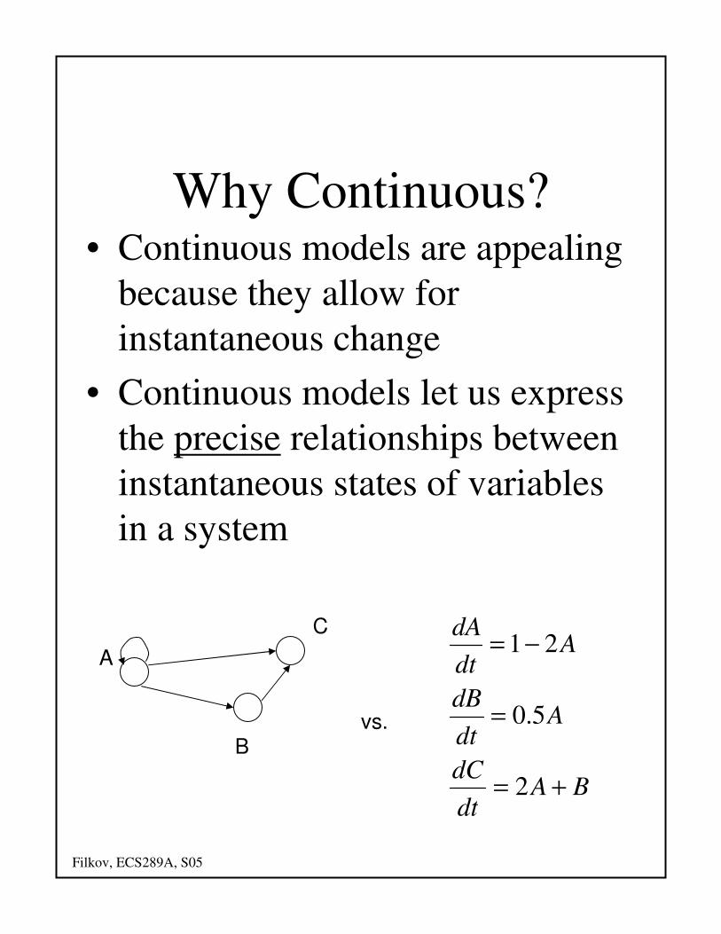
Why Continuous?• Continuous models are appealing

because they allow for

instantaneous change

• Continuous models let us express

the precise relationships between

instantaneous states of variables

in a system

A

B

C

vs.

BAdt

dC

Adt

dB

Adt

dA

+=

=

−=

2

5.0

21


ProblemsWhen modeling with differential equations we face all the same problems as in the discrete models:

– Posing the equations. This presumes we understand the underlying phenomenon

– Data Fitting. How do we learn the model from the data?

– Solving the equations. Means we can do the math

– Model Behavior. Analyzing the fitted model to understand its behavior


Recall the Modeling

Process…1. Knowledge

2. Modeling Objectives

3. Construct and Revise Models

4. Model behavior and

predictions

5. Compare to new data

6. Better Models, goto 3

7. Learn…


1. Ordinary Differential

Equations

Rate equation:

function a is :)(

]x,,[x

where

1 ),(

ionsconcentrat of vector a isn1

RR

x

x

→

=

≤≤=

n

i

n

i

i

xf

nifdt

dx

K

Systems of ODEs: There are n such equations

Solving the rate equations depends on f, but what is the form of the function f ?

The answer is: as simple as possible.


• The rate function specifies the interactions

between the state variables.

• Its input are the concentrations, and the output

is indicative (i.e. a function of) the change in a

gene’s regulation

• The regulation function describes how the

concentration is related to regulation

• This is a typical regulation function, called a

sigmoid, bellow compared to similar ones

The Rate Function and

Regulation


Non-linear ODEs

The rate function is nonlinear!

Eg.

1. Sigmoidal

2. Nonlinear, additive. Summarizes all

pair wise (and nothing but pair wise)

relationship

3. Nonlinear, non-additive. Summarizes

all pairs and triplets of relationships

∑∑ +=j

jjij

jk

kkjjijk

i XfTXfXfTdt

dX)()()(

∑=j

jjij

i XfTdt

dX)(


Solving

• In general, these equations are difficult to

solve analytically when fi(x) are non-linear

• Numerical Simulators/Solvers work by

numerically approximating the

concentration values at discretized,

consecutive time-points. Popular software

for biochemical interactions:

– DBsolve

– GEPASI

– MIST

– SCAMP

• Although analytical solutions are

impossible, we can learn a lot from general

analyses of the behavior of the models,

which some of the packages above provide


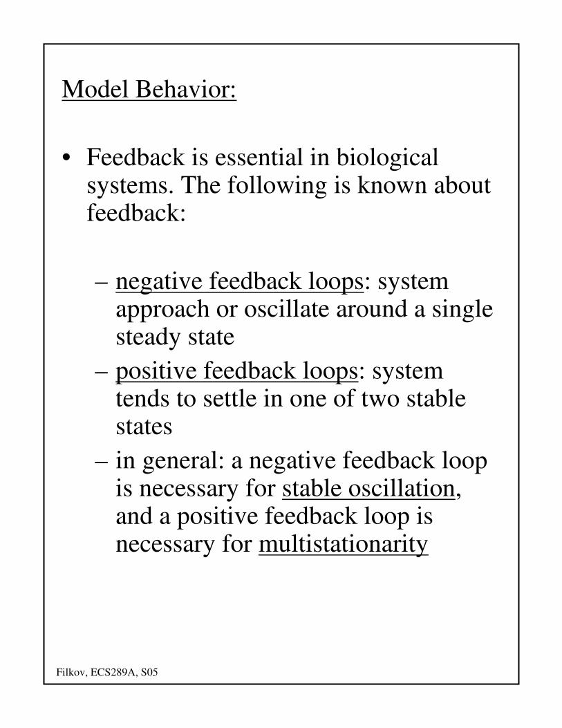
Model Behavior:

• Feedback is essential in biological systems. The following is known about feedback:

– negative feedback loops: system approach or oscillate around a single steady state

– positive feedback loops: system tends to settle in one of two stable states

– in general: a negative feedback loop is necessary for stable oscillation, and a positive feedback loop is necessary for multistationarity


Data Fitting

• Fitting the parameters of a non-linear system is a difficult problem.

• Common solution: non-linear optimization scheme

– explore the parameter space of the system

– for each choice of parameters the models are solved numerically (e.g. Runge-Kutta)

– the parameterized model is compared to the data with a goodness of fit function. It is this function that is optimized

• Genetic Algorithms and Simulated Annealing, with proper transition functions have been used with promising results


Linear and Piecewise Linear

ODEs

Linear

– These are much easier to deal with:

if the input variables are limited by

a constant, they can be solved and

learned polynomially, depending on

the amount of data available

– One way to learn them is by

approximating them with linear

weight models

∑=j

jij

i Xwdt

dX


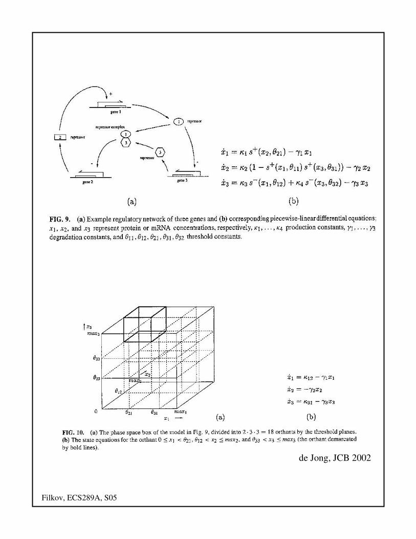
Piecewise linear

• Approximating the sigmoid regulatory

function with a step function

• Here the function bil is a function of n

variables, defined in terms of sums and

products of step functions:

• This amounts to subdividing n-dimensional

space into “orthants”, and in each of the

orthants the PLODEs reduce to ODEs

∑∈

≥=

≤≤−=

Ll

ilili

iii

i

bkg

xgdt

dX

0)()(

ni1 ,)(

xx

x γ

0

1

jθ

0

1

kθ


de Jong, JCB 2002


2. PDES

• ODEs count on spatial homogeneity

• In other words, ODEs don’t care where the processes take place

• But in some real situation this assumption clearly does not hold

– Diffusion

– Transcription factor gradients in development

– Multicelular organisms


Example: Reaction-

Diffusion Equations

The equation above describes the change in conc. for

all state variables, in all cells of the line above. When

the number of cells is large, this becomes a PDE:

These equations were first introduced in the study of

developmental phenomena and pattern formation by

Turing.

Direct analytical solutions are impossible even for two

variables (n=2)


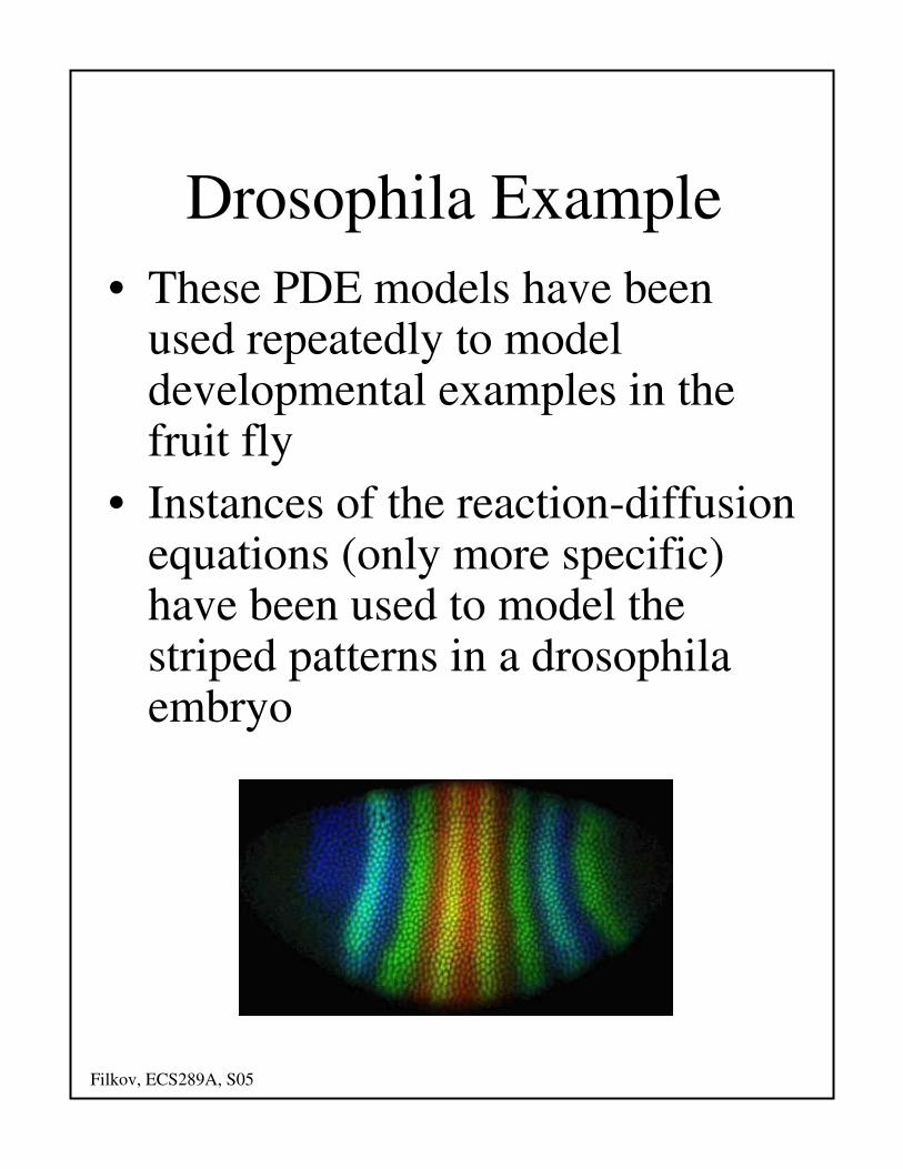
Drosophila Example

• These PDE models have been used repeatedly to model developmental examples in the fruit fly

• Instances of the reaction-diffusion equations (only more specific) have been used to model the striped patterns in a drosophila embryo


3. Stochastic Master

Equations

• Deterministic modeling is not always possible, but also sometimes incorrect

• Assumptions of deterministic, continuous models:– Concentrations of substances vary

deterministically

– Conc. Of subst. vary continuously

• On molecular level, both assumptions may not be correct

• Solution: Instead of deterministic values, accept a joint probability distribution, similar to the one discussed in the Bayesian Network lectures.


Equation:

These equations are very difficult to solve and simulate!

ODE vs. Stochastic solutions

(c) Jason Kastner and Caltech


Linear (Weight Matrix)

Models of Regulation


Description of the Model• A graph model in which the nodes are genes

that are in continuous states of expression (i.e.

gene activities). The edges indicate the strength

(weight) of the regulation relationship between

two genes

• The net effect of gene j on gene i is the

expression level of gene j multiplied by its

regulatory influence on i, i.e. wijxj.

• Assumptions:

– regulators’ contribution to a gene’s

regulation is linearly additive

– the states of the nodes are updated

synchronously

A B

C

D

xa(t)

xc(t)

xb(t)

xd(t)

wc,bwa,c

wa,d

wd,c wb,d

xi(t) – state of gene i at time t

wij – regulatory influence of

gene j on gene i

- wij > 0, activation

- wij < 0, inhibition

- wij = 0, none


Calculating the Next

State of the System

If all the weights, wij are known,

then given the activities of all

the genes at time t, i.e.

x1(t),x2(t),…,xn(t), we can

calculate the activities of the

genes at time t+1.

)1()()1(

1

,

:notationmatrix in Or

,

)()1(1

×××

+ ⋅=

∈

∑=+=

n

t

nnn

t

jii

jiji

wx

txwtxn

j

xWx

R


Fitting the Model to the Data

• In reality, we don’t know the weights, and we would like to infer them from measurements of the activities of genes through time (microarray data)

• The weights can be found by solving a system of linear equations (multiple regression)

• Dimensionality Curse: the expression matrices, of size n x k, where n is in thousands and k is at most in hundreds

• The linear system is always under-constrained and thus yields infinitely many solutions (compare to over-constrained where we need to use least-squares fit)


[ ]

1)T(AATA** AA,**AW

TA1A)T(A** AB,**AW

iy

A

W

n)(kB

n)(kA

iy

iy

BTWA

1ky

3y

2y

B

ky

2y

1y

A

−==

−==

=

<

=

>

×

×

+=+

=•

+

=

=

:as Penrose),-(Moore data thefitsbest that toinverse

-pseudo a findcan Wesolutions.many infinitely are

thereand rained,underconst is system the, If

solution; unique a is there If

:solution n)(regressio squaresleast A solution. unique no is

thereand ained,overconstr is system the, If

for solve want to which we,

:becomes systemlinear theThen,

.i.e. vectors,last the toequal rowsh matrix wit a be

and , i.e. vectors,first the toequal rowsh matrix wit a be

let,11 , vectorsi.e. points, time1given Then,

i.e. i,point at time genes of sexpression therepresent vector Let the

. )()(2

)(1

nk

nk

nk

k

k

,...,k i k

n

in

xixix

L

L

L

Solving the Linear Model


Normalization

• The input gene expressions

need to be normalized at each

step, so that the contributions

are comparable across all genes

• The resulting (output) values

are then de-normalized

• Common normalization

schemes:

– mean/variance: x’=(x-µ)/σ2

– Squashing function: (neural nets)


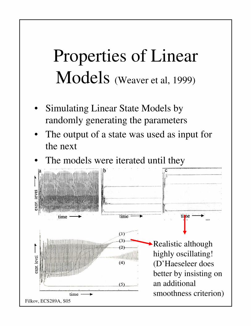
Properties of Linear

Models (Weaver et al, 1999)

• Simulating Linear State Models by

randomly generating the parameters

• The output of a state was used as input for

the next

• The models were iterated until they

reached a terminal steady state

Realistic although

highly oscillating!

(D’Haeseleer does

better by insisting on

an additional

smoothness criterion)


Limitations

• Some assumptions are known to be incorrect:

– all genetic interactions are independent events

– synchronous dynamics

– weight matrix

• The results may not offer insight to the problem instead they may just model the data well (the weight matrix will be chosen based on multiple regression)


How Much Data?

• If the weight matrix is dense, we

need n+1 arrays of all n genes to

solve the linear system, assuming the

experiments are independent (which

is not exactly true with time-series

data). In this case we say that the

average connectivity is O(n) per

node.

• If instead the average connectivity

per node is fixed to O(p), than it can

be shown that the number of

experiments needed is

O(p*log(n/p))


Summary

• Linear models yield good, realistic

looking predictions

• The amount of data needed is O(n)

experiments, for a fully connected

network or O(p*log(n/p)) for a p-

connected network

• The weight matrix can be obtained by

solving a linear system of equations

• Dimensionality curse: more genes

than experiments. We have to resort

to reducing the dimensionality of the

problem (e.g. through clustering)


Biography

• Hidde de Jong, Modeling and Simulation of Genetic Regulatory Systems:

A Literature Review. Journal of Computational Biology 9(1): 67-103

(2002).

• McAdams and Arkin, Annu. Rev. Biophys. Biomol. Struct. 1998 (27)

• Setty, Y. et al., Detailed map of a cis-regulatory input function, PNAS,

100:7702-7707 (2003)

• Fangting et al., PNAS 2004 (101)

• Albert, R. and Othmer, H.G. Journal of Theoretical Biology 223, 1-18

(2003).

• Davidson, E.H. et al., Science 295, 1669-1678, 2002

• D. C. Weaver and C. T. Workman and G. D. Stromo, Pacific Symposium

on Biocomputing, 1999.

• D’Haeseleer et al., Pacific Symposium on Biocomputing, 1999.

biological networks - web.cs.ucdavis.edu

Documents